Robust Learning Through Cross-Task Consistency
通过跨任务一致性实现稳健学习
Abstract
摘要
Visual perception entails solving a wide set of tasks, e.g., object detection, depth estimation, etc. The predictions made for multiple tasks from the same image are not independent, and therefore, are expected to be ‘consistent’. We propose a broadly applicable and fully computational method for augmenting learning with Cross-Task Consistency.1 The proposed formulation is based on inference-path invariance over a graph of arbitrary tasks. We observe that learning with cross-task consistency leads to more accurate predictions and better generalization to out-of-distribution inputs. This framework also leads to an informative unsupervised quantity, called Consistency Energy, based on measuring the intrinsic consistency of the system. Consistency Energy correlates well with the supervised error $'r{=}0.67,$ , thus it can be employed as an unsupervised confidence metric as well as for detection of out-of-distribution inputs $R O C-A U C=0.95$ ). The evaluations are performed on multiple datasets, including Taskonomy, Replica, CocoDoom, and ApolloS cape, and they benchmark cross-task consistency versus various baselines including conventional multi-task learning, cycle consistency, and analytical consistency.
视觉感知涉及解决一系列广泛的任务,例如目标检测、深度估计等。同一图像上多个任务的预测并非独立,因此应保持"一致性"。我们提出了一种通用且完全基于计算的方法,通过跨任务一致性 (Cross-Task Consistency) 来增强学习效果。该方案基于任意任务图上的推理路径不变性。实验表明,跨任务一致性学习能提高预测精度,并增强对分布外输入的泛化能力。该框架还衍生出一个称为一致性能量 (Consistency Energy) 的无监督指标,通过测量系统内在一致性实现。一致性能量与监督误差高度相关 $'r{=}0.67,$ ,可作为无监督置信度度量及分布外输入检测指标 $R O C-A U C=0.95$ )。评估在Taskonomy、Replica、CocoDoom和ApolloS cape等多个数据集上进行,将跨任务一致性与传统多任务学习、循环一致性和解析一致性等基线方法进行了对比。
1. Introduction
1. 引言
What is consistency: suppose an object detector detects a ball in a particular region of an image, while a depth estimator returns a flat surface for the same region. This presents an issue – at least one of them has to be wrong, because they are inconsistent. More concretely, the first prediction domain (objects) and the second prediction domain (depth) are not independent and consequently enforce some constraints on each other, often referred to as consistency constraints.
一致性是什么:假设一个物体检测器在图像的某个区域检测到一个球,而深度估计器却对同一区域返回了一个平面。这就产生了一个问题——至少有一个结果是错误的,因为它们是不一致的。更具体地说,第一个预测域(物体)和第二个预测域(深度)并非相互独立,因此彼此之间存在某些约束,通常被称为一致性约束。
Why is it important to incorporate consistency in learning: first, desired learning tasks are usually predictions of different aspects of one underlying reality (the scene that underlies an image). Hence inconsistency among predictions implies contradiction and is inherently undesirable. Second, consistency constraints are informative and can be used to better fit the data or lower the sample complexity. Also, they may reduce the tendency of neural networks to learn “surface statistics” (superficial cues) [18], by enforcing constraints rooted in different physical or geometric rules. This is empirically supported by the improved generalization of models when trained with consistency constraints (Sec. 5).
为什么在学习中保持一致性很重要:首先,理想的学习任务通常是对同一潜在现实(如图像背后的场景)不同方面的预测。因此,预测间的不一致意味着矛盾,本质上是不理想的。其次,一致性约束具有信息量,可用于更好地拟合数据或降低样本复杂度。此外,通过强制实施基于不同物理或几何规则的约束,它们可能减少神经网络学习"表面统计量"(浅层线索)的倾向[18]。这一点在经验上得到了支持,即使用一致性约束训练的模型具有更好的泛化能力(见第5节)。
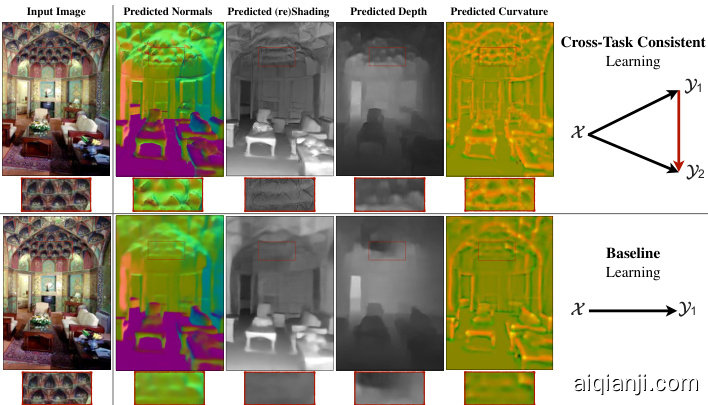
Figure 1: Cross-Task Consistent Learning. The predictions made for different tasks out of one image are expected to be consistent, as the underlying scene is the same. This is exemplified by a challenging query and four sample predictions out of it. We propose a general method for learning utilizing data-driven cross-task consistency constraints. The lower and upper rows show the results of the baseline (independent learning) and learning with consistency, which yields higher quality and more consistent predictions. Red boxes provide magnifications. [Best seen on screen]
图 1: 跨任务一致性学习。由于底层场景相同,对同一图像不同任务的预测结果应保持一致性。图中展示了一个具有挑战性的查询及其四个预测示例。我们提出了一种利用数据驱动的跨任务一致性约束进行学习的通用方法。下方和上方两行分别展示了基线(独立学习)和采用一致性学习的结果,后者能产生更高质量且更一致的预测。红色方框为局部放大区域。[建议屏幕观看]
How can we design a learning system that makes consistent predictions: this paper proposes a method which, given an arbitrary dictionary of tasks, augments the learning objective with explicit constraints for cross-task consistency. The constraints are learned from data rather than apriori given relationships.2 This makes the method applicable to any pairs of tasks as long as they are not statistically independent; even if their analytical relationship is unknown, hard to program, or non-differentiable. The primary concept behind the method is ‘inference-path invariance’. That is, the result of inferring an output domain from an input domain should be the same, regardless of the intermediate domains mediating the inference (e.g., RGB $\rightarrow$ normals and RGB $\rightarrow$ depth $\rightarrow$ normals and RGB $\rightarrow$ shading $\rightarrow$ normals are expected to yield the same normal results). When inference paths with the same endpoints, but different intermediate domains, yield similar results, this implies the intermediate domain predictions did not conflict as far as the output was concerned. We apply this concept over paths in a graph of tasks, where the nodes and edges are prediction domains and neural network mappings between them, respectively (Fig. 2(d)). Satisfying this invariance constraint over all paths in the graph ensures the predictions for all domains are in global cross-task agreement.3
如何设计一个能做出一致预测的学习系统:本文提出了一种方法,在给定任意任务字典的情况下,通过显式的跨任务一致性约束来增强学习目标。这些约束是从数据中学习得到的,而非预先给定的关系。这使得该方法适用于任何统计上不独立的成对任务,即使它们的解析关系未知、难以编程或不可微分。
该方法的核心概念是"推理路径不变性"。即无论推理过程中经过哪些中间域(例如 RGB→法线、RGB→深度→法线、RGB→着色→法线),从输入域推断输出域的结果都应相同。当具有相同端点但不同中间域的推理路径产生相似结果时,就意味着这些中间域的预测在输出层面没有产生冲突。我们将这一概念应用于任务图中的路径,其中节点表示预测域,边表示它们之间的神经网络映射(图 2(d))。满足图中所有路径的这种不变性约束,就能确保所有域的预测达到全局跨任务一致性。
To make the associated large optimization job manageable, we reduce the problem to a ‘separable’ one, devise a tractable training schedule, and use a ‘perceptual loss’ based formulation. The last enables mitigating residual errors in networks and potential ill-posed/one-to-many mappings between domains (Sec. 3).
为了使相关的大规模优化任务变得可管理,我们将问题简化为一个"可分离"的问题,设计了一个易于处理的训练计划,并采用了基于"感知损失"的公式。最后一项措施有助于减轻网络中的残余误差以及领域间潜在的病态/一对多映射问题(第3节)。
Interactive visualization s, trained models, code, and a live demo are available at http://consistency.epfl.ch/.
交互式可视化工具、训练好的模型、代码和实时演示可在 http://consistency.epfl.ch/ 获取。
2. Related Work
2. 相关工作
The concept of consistency and methods for enforcing it are related to various topics, including structured prediction, graphical models [22], functional maps [30], and certain topics in vector calculus and differential topology [10]. We review the most relevant ones in context of computer vision.
一致性的概念及其实现方法涉及多个相关领域,包括结构化预测、图模型 [22]、函数映射 [30] ,以及向量微积分和微分拓扑中的某些主题 [10]。我们将在计算机视觉的背景下回顾其中最相关的内容。
Utilizing consistency: Various consistency constraints have been commonly found beneficial across different fields, e.g., in language as ‘back-translation’ [2, 1, 25, 7] or in vision over the temporal domain [41, 6], 3D geometry [9, 32, 8, 13, 49, 46, 15, 44, 51, 48, 23, 5], and in recognition and (conditional/unconditional) image translation [12, 28, 17, 50, 14, 4]. In computer vision, consistency has been extensively utilized in the cycle form and often between two or few domains [50, 14]. In contrast, we consider consistency in the more general form of arbitrary paths with varied-lengths over a large task set, rather than the special cases of short cyclic paths. Also, the proposed approach needs no prior explicit knowledge about task relationships [32, 23, 44, 51].
利用一致性:各种一致性约束在不同领域中被普遍认为是有益的,例如在语言中的"回译" [2, 1, 25, 7] 或在视觉中的时间域 [41, 6]、3D几何 [9, 32, 8, 13, 49, 46, 15, 44, 51, 48, 23, 5],以及识别和(条件/无条件)图像转换 [12, 28, 17, 50, 14, 4]。在计算机视觉中,一致性已被广泛用于循环形式,并且通常在两个或少数几个域之间 [50, 14]。相比之下,我们考虑的是更一般形式的一致性,即在大型任务集上具有不同长度的任意路径,而不是短循环路径的特殊情况。此外,所提出的方法不需要事先明确了解任务关系 [32, 23, 44, 51]。
Multi-task learning: In the most conventional form, multi-task learning predicts multiple output domains out of a shared encoder/representation for an input. It has been speculated that the predictions of a multi-task network may be automatically cross-task consistent as the represent ation from which the predictions are made are shared. This has been observed to not be necessarily true in several works [21, 47, 43, 38], as consistency is not directly enforced during training. We also make the same observation (see visuals here) and quantify it (see Fig. 9(a)), which signifies the need for explicit augmentation of consistency in learning.
多任务学习:在最常见的形式中,多任务学习通过共享的编码器/表示对输入预测多个输出域。有推测认为,由于预测基于共享表示,多任务网络的预测可能自动实现跨任务一致性。但多项研究[21, 47, 43, 38]发现这并不必然成立,因为训练过程中并未直接强制一致性。我们同样观察到这一现象(参见可视化示例)并进行了量化分析(见图9(a)),这表明需要在学习中显式增强一致性。

Figure 2: Enforcing Cross-Task Consistency: (a) shows the typical multitask setup where predictions and $\scriptstyle\mathcal{X}\to\mathcal{Y}{2}$ are trained without a notation of consistency. (b) depicts the elementary triangle consistency constraint where the prediction is enforced to be consistent with $\scriptstyle\mathcal{X}\to\mathcal{Y}{2}$ using a function that relates ${\textrm{y}{1}}$ to ${\mathcal{V}{2}}$ (i.e. $y_{1}{\rightarrow}y_{2}$ ). (c) shows how the triangle unit from (b) can be an element of a larger system of domains. Finally, (d) illustrates the generalized case where in the larger system of domains, consistency can be enforced using invariance along arbitrary paths, as long as their endpoints are the same (here the blue and green paths). This is the general concept behind inference-path invariance. The triangle in (b) is the smallest unit of such paths.
图 2: 跨任务一致性约束: (a)展示典型的多任务设置,其中预测和$\scriptstyle\mathcal{X}\to\mathcal{Y}{2}$在没有一致性概念的情况下进行训练。(b)描述基础三角一致性约束,通过关联${\textrm{y}{1}}$和${\mathcal{V}{2}}$的函数(即$y_{1}{\rightarrow}y_{2}$)强制使预测与$\scriptstyle\mathcal{X}\to\mathcal{Y}_{2}$保持一致。(c)展示(b)中的三角单元如何成为更大领域系统的组成部分。(d)说明广义情况:在更大的领域系统中,只要路径端点相同(图中蓝色与绿色路径),即可通过任意路径上的不变性来实施一致性。这是推理路径不变性背后的核心思想,而(b)中的三角是此类路径的最小单元。
Transfer learning predicts the output of a target task given another task’s solution as a source. The predictions made using transfer learning are sometimes assumed to be cross-task consistent, which is often found to not be the case [45, 36], as transfer learning does not have a specific mechanism to impose consistency by default. Unlike basic multi-task learning and transfer learning, the proposed method includes explicit mechanisms for learning with general data-driven consistency constraints.
迁移学习通过将一个任务的解决方案作为源来预测目标任务的输出。使用迁移学习做出的预测有时被假定为跨任务一致的,但实际情况往往并非如此 [45, 36],因为迁移学习默认不具备强制一致性的特定机制。与基础的多任务学习和迁移学习不同,所提出的方法包含明确的机制,用于在通用数据驱动的一致性约束下进行学习。
Uncertainty metrics: Among the existing approaches to measuring prediction uncertainty, the proposed Consistency Energy (Sec. 4) is most related to Ensemble Averaging [24], with the key difference that the estimations in our ensemble are from different cues/paths, rather than retraining/reevaluating the same network with different random initi aliz at ions or parameters. Using multiple cues is expected to make the ensemble more effective at capturing uncertainty.
不确定性度量:在现有的预测不确定性测量方法中,提出的Consistency Energy(第4节)与Ensemble Averaging [24]最为相关,关键区别在于我们的集成估计来自不同线索/路径,而非通过不同随机初始化或参数重新训练/评估同一网络。使用多线索有望使集成在捕捉不确定性方面更有效。
3. Method
3. 方法
We define the problem as follows: suppose $\mathcal{X}$ denotes the query domain (e.g., RGB images) and $y={y_{1},...,y_{n}}$ is the set of $n$ desired prediction domains (e.g. normals, depth, objects, etc). An individual datapoint from domains $\left(x,y_{1},...,y_{n}\right)$ is denoted by $(x,y_{1},...,y_{n})$ . The goal is to learn functions that map the query domain onto the prediction domains, i.e. $\mathcal{F}{\boldsymbol{x}}={f_{\boldsymbol{x}\mathscr{y}{j}}|\boldsymbol{y}{j}\in\boldsymbol{y}}$ where $f_{x y_{j}}(x)$ out- puts $y_{j}$ given $x$ . We also define $\mathcal{F}{y}{=}{f_{\mathcal{V}{i}\mathcal{V}{j}}|y_{i},y_{j}{\in}y,i{\neq}j}$ , which is the set of ‘cross-task’ functions that map the prediction domains onto each other; we use them in the consistency constraints. For now assume $\mathcal{F}{y}$ is given apriori and frozen; in Sec. 3.3 we discuss all functions $f\mathrm{s}$ are neural networks in this paper, and we learn $\mathcal{F}{y}$ just like ${\mathcal{F}}_{\mathcal{X}}$ .
我们将问题定义如下:假设$\mathcal{X}$表示查询域(例如RGB图像),$y={y_{1},...,y_{n}}$是$n$个目标预测域(例如法线、深度、物体等)的集合。来自域$\left(x,y_{1},...,y_{n}\right)$的单个数据点记为$(x,y_{1},...,y_{n})$。目标是学习将查询域映射到预测域的函数,即$\mathcal{F}{\boldsymbol{x}}={f_{\boldsymbol{x}\mathscr{y}{j}}|\boldsymbol{y}{j}\in\boldsymbol{y}}$,其中$f_{x y_{j}}(x)$在给定$x$时输出$y_{j}$。我们还定义了$\mathcal{F}{y}{=}{f_{\mathcal{V}{i}\mathcal{V}{j}}|y_{i},y_{j}{\in}y,i{\neq}j}$,这是将预测域相互映射的"跨任务"函数集合,用于一致性约束。目前假设$\mathcal{F}{y}$是预先给定且固定的;在第3.3节中,我们将讨论本文中所有函数$f\mathrm{s}$都是神经网络,并且像${\mathcal{F}}{\mathcal{X}}$一样学习$\mathcal{F}_{y}$。
3.1. Triangle: The Elementary Consistency Unit
3.1. Triangle: 基本一致性单元
A common way of training neural networks in ${\mathcal{F}}{\mathcal{X}}$ , e.g. $f_{x y_{1}}(x)$ , is to find parameters of $f_{\boldsymbol{\mathcal{X}}\mathcal{y}{1}}$ that minimize a loss of the form $\left|f_{\chi y_{1}}(x)-y_{1}\right|$ using a common distance function as $|.|.$ , e.g. $\ell_{1}$ norm. This standard independent learning of $f_{\boldsymbol{\mathcal{X}}\boldsymbol{\mathcal{y}}{i}}\mathrm{s}$ satisfies various desirable properties, including crosstask consistency, if given infinite amount of data, but not under the practical finite data regime. This is shown in Fig. 3 (upper). Thus we introduce additional constraints to guide the training toward cross-task consistency. We define the loss for predicting domain $y_{1}$ from $\mathcal{X}$ while enforcing consistency with domain $y_{2}$ as a directed triangle depicted in Fig. 2(b):
在 ${\mathcal{F}}{\mathcal{X}}$ 中训练神经网络的常见方法,例如 $f_{x y_{1}}(x)$,是通过寻找 $f_{\boldsymbol{\mathcal{X}}\mathcal{y}{1}}$ 的参数,以最小化形如 $\left|f_{\chi y_{1}}(x)-y_{1}\right|$ 的损失,并使用常见的距离函数如 $|.|.$,例如 $\ell_{1}$ 范数。这种对 $f_{\boldsymbol{\mathcal{X}}\boldsymbol{\mathcal{y}}{i}}\mathrm{s}$ 的标准独立学习在给定无限数据量时满足包括跨任务一致性在内的各种理想特性,但在实际有限数据情况下则不然。如图 3(上)所示。因此,我们引入额外的约束来引导训练实现跨任务一致性。我们将从 $\mathcal{X}$ 预测域 $y_{1}$ 同时强制与域 $y_{2}$ 一致的损失定义为图 2(b) 中所示的有向三角形:
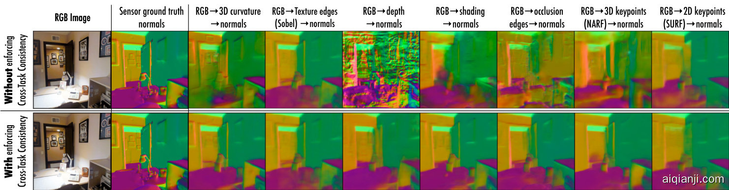
Figure 3: Impact of disregarding cross-task consistency in learning, illustrated using surface normals domain. Each subfigure shows the results of predicting surface normals out of the prediction of an intermediate domain; using the notation $x{\to}y_{1}{\to}y_{2}$ , here ${\mathscr{X}}$ is RGB image, ${3/2}$ is surface normals, and each column represents a different ${\gg_{1}}$ . The upper row demonstrates the normals are noisy and dissimilar when cross-task consistency is not incorporated in learning of networks. Whereas enforcing consistency when learning results in more consistent and better normals (the lower row). We will show this causes the predictions for the intermediate domains themselves to be more accurate and consistent. More examples available in supplementary material. The Consistency Energy (Sec. 4) captures the variance among predictions in each row.
图 3: 忽略跨任务一致性对学习的影响,以表面法线域为例进行说明。每个子图展示了通过中间域预测结果推导表面法线的效果;使用符号$x{\to}y_{1}{\to}y_{2}$表示,其中${\mathscr{X}}$为RGB图像,${3/2}$为表面法线,每列代表不同的。上排显示当网络学习过程中未纳入跨任务一致性时,法线预测结果存在噪声且不一致。而下排表明在学习时强制保持一致性,可获得更一致且更优的法线结果。我们将证明这会使中间域自身的预测更准确和一致。补充材料提供更多示例。一致性能量(第4节)量化了每行预测结果的方差。
$$
\mathcal{L}{\chi\nu_{1}\nu_{2}}^{t r i a n g l e}\triangleq\left|f_{\chi\nu_{1}}(x)-y_{1}|+|f_{\mathcal{V}{1}\mathcal{V}{2}}\circ f_{\chi\nu_{1}}(x)-f_{\chi\nu_{2}}(x)|+|f_{\chi\nu_{2}}(x)-y_{2}|.\right.
$$
$$
\mathcal{L}{\chi\nu_{1}\nu_{2}}^{t r i a n g l e}\triangleq\left|f_{\chi\nu_{1}}(x)-y_{1}|+|f_{\mathcal{V}{1}\mathcal{V}{2}}\circ f_{\chi\nu_{1}}(x)-f_{\chi\nu_{2}}(x)|+|f_{\chi\nu_{2}}(x)-y_{2}|.\right.
$$
The first and last terms are the standard direct losses for training $f_{\boldsymbol{\mathcal{X}}\boldsymbol{\mathcal{y}}{1}}$ and $f_{\boldsymbol{{x y}}{2}}$ . The middle term is the consistency term which enforces predicting $y_{2}$ out of the predicted $y_{1}$ yields the same result as directly predicting $y_{2}$ out of $\chi^{4}$ . Thus learning to predict $y_{1}$ and $y_{2}$ are not independent anymore.
首尾两项分别是训练 $f_{\boldsymbol{\mathcal{X}}\boldsymbol{\mathcal{y}}{1}}$ 和 $f_{\boldsymbol{{x y}}{2}}$ 的标准直接损失。中间项是一致性约束项,强制要求通过预测出的 $y_{1}$ 来预测 $y_{2}$ 的结果,应与直接从 $\chi^{4}$ 预测 $y_{2}$ 的结果一致。因此学习预测 $y_{1}$ 和 $y_{2}$ 的过程不再相互独立。
The triangle loss 1 is the smallest unit of enforcing crosstask consistency. Below we make two improving modifications on it via function ‘se par ability’ and ‘perceptual losses’.
三角损失1是实施跨任务一致性的最小单元。下面我们通过函数的"可分性"和"感知损失"对其进行两项改进。
3.1.1 Se par ability of Optimization Parameters
3.1.1 优化参数的可分离性
The loss $\mathcal{L}{\mathcal{X}\mathcal{Y}{1}\mathcal{Y}{2}}^{t r i a n g l e}$ involves simultaneous training of two networks $f_{\boldsymbol{\mathcal{X}}\boldsymbol{\mathcal{y}}{1}}$ and $f_{\boldsymbol{{x y}}_{2}}$ , thus it is resource demanding. We show Ltriangle can be reduced to a ‘separable’ function [39] resulting in two terms that can be optimized independently.
损失 $\mathcal{L}{\mathcal{X}\mathcal{Y}{1}\mathcal{Y}{2}}^{triangle}$ 涉及同时训练两个网络 $f_{\boldsymbol{\mathcal{X}}\boldsymbol{\mathcal{y}}{1}}$ 和 $f_{\boldsymbol{{x y}}_{2}}$ ,因此对资源要求较高。我们证明 Ltriangle 可简化为一个"可分离"函数 [39],从而得到两个可独立优化的项。
From triangle inequality we can derive:
由三角不等式可得:
$$
\mid f_{y_{1}y_{2}}\circ f_{x y_{1}}(x)-f_{x y_{2}}(x)\mid\leq\mid f_{y_{1}y_{2}}\circ f_{x y_{1}}(x)-y_{2}\mid+\mid f_{x y_{2}}(x)-y_{2}\mid,
$$
$$
\mid f_{y_{1}y_{2}}\circ f_{x y_{1}}(x)-f_{x y_{2}}(x)\mid\leq\mid f_{y_{1}y_{2}}\circ f_{x y_{1}}(x)-y_{2}\mid+\mid f_{x y_{2}}(x)-y_{2}\mid,
$$
which after substitution in Eq. 1 yields:
代入式1后可得:
$$
\mathcal{L}{\chi\ni_{1}\chi_{2}}^{t r i a n g l e}\leq\left|f_{\chi\ni_{1}}(x)-y_{1}\right|+\left|f_{\mathcal{V}{1}\mathcal{V}{2}}\circ f_{\chi_{\mathcal{V}{1}}}(x)-y_{2}\right|+2\left|f_{\chi\mathcal{V}{2}}(x)-y_{2}\right|.
$$
$$
\mathcal{L}{\chi\ni_{1}\chi_{2}}^{t r i a n g l e}\leq\left|f_{\chi\ni_{1}}(x)-y_{1}\right|+\left|f_{\mathcal{V}{1}\mathcal{V}{2}}\circ f_{\chi_{\mathcal{V}{1}}}(x)-y_{2}\right|+2\left|f_{\chi\mathcal{V}{2}}(x)-y_{2}\right|.
$$
The upper bound for $\mathcal{L}{\mathcal{X}\mathcal{Y}{1}\mathcal{Y}{2}}^{t r i a n g l e}$ in inequality 2 can be optimized in lieu of $\mathcal{L}{\mathcal{X}\mathcal{Y}{1}\mathcal{Y}{2}}^{t r i a n g l e}$ its1el2f, as they both have the same minimizer.5 The terms of this bound include either $f_{\boldsymbol{\mathcal{X}}\boldsymbol{\mathcal{y}}_{1}}$
不等式2中 $\mathcal{L}{\mathcal{X}\mathcal{Y}{1}\mathcal{Y}{2}}^{triangle}$ 的上界可以替代 $\mathcal{L}{\mathcal{X}\mathcal{Y}{1}\mathcal{Y}{2}}^{triangle}$ 本身进行优化,因为两者具有相同的最小化点。该上界的各项包含 $f_{\boldsymbol{\mathcal{X}}\boldsymbol{\mathcal{y}}_{1}}$
or $f_{\boldsymbol{{x y}}{2}}$ , but not both, hence we now have a loss separable into functions of $f_{\boldsymbol{\mathcal{X}}\boldsymbol{\mathcal{y}}{1}}$ or $f_{\boldsymbol{\mathcal{X}}\boldsymbol{\mathcal{Y}}{2}}$ , and they can be optimized independently. The part pertinent to the network $f_{\boldsymbol{\mathcal{X}}\boldsymbol{\mathcal{y}}_{1}}$ is:
或 $f_{\boldsymbol{{x y}}{2}}$,但不能同时优化两者,因此现在我们可以将损失函数分离为 $f_{\boldsymbol{\mathcal{X}}\boldsymbol{\mathcal{y}}{1}}$ 或 $f_{\boldsymbol{\mathcal{X}}\boldsymbol{\mathcal{Y}}{2}}$ 的函数,并且可以独立优化。与网络 $f_{\boldsymbol{\mathcal{X}}\boldsymbol{\mathcal{y}}_{1}}$ 相关的部分为:
$$
\mathcal{L}{x y_{1}y_{2}}^{s e p a r a t e}\overset{\Delta}{=}|f_{x y_{1}}(x)-y_{1}|+|f_{y_{1}y_{2}\circ{}}f_{x y_{1}}(x)-y_{2}|,
$$
$$
\mathcal{L}{x y_{1}y_{2}}^{s e p a r a t e}\overset{\Delta}{=}|f_{x y_{1}}(x)-y_{1}|+|f_{y_{1}y_{2}\circ{}}f_{x y_{1}}(x)-y_{2}|,
$$
named separate, as we reduced the closed triangle objective $\chi\stackrel{\star_{1}}{\Delta}y_{2}$ ${\textrm{y}{1}}$ in Eq. 1 to two equivalent separate path objectives $x{\to}y_{1}{\to}y_{2}$ and $\chi{\rightarrow}{\gg}{2}$ . The first term of Eq. 3 enforces the general correctness of predicting $y_{1}$ , and the second term enforces its consistency with $_{\mathcal{V}2}$ domain.
将闭合三角形目标 $\chi\stackrel{\star_{1}}{\Delta}y_{2}$ ${\textrm{y}{1}}$ 在公式1中拆分为两个等效的独立路径目标 $x{\to}y_{1}{\to}y_{2}$ 和 $\chi{\rightarrow}{\gg}{2}$ 。公式3的第一项确保预测 $y_{1}$ 的总体正确性,第二项强制其与 $_{\mathcal{V}2}$ 域的一致性。
3.1.2 Reconfiguration into a “Perceptual Loss”
3.1.2 重构为"感知损失"
Training $f_{\boldsymbol{\mathcal{X}}\boldsymbol{\mathcal{y}}{1}}$ using the loss $\mathcal{L}{\mathcal{X}\mathcal{Y}{1}\mathcal{Y}{2}}^{s e p a r a t e}$ requires a training dataset with multi domain annotations for one input: $(x,y_{1},y_{2})$ . It also relies on availability of a perfect function $f_{y_{1}y_{2}}$ for mapping $y_{1}$ onto $y_{2}$ ; i.e. it demands $y_{2}{=}f_{y_{1}y_{2}}(y_{1})$ . We show how these two requirements can be reduced.
使用损失函数 $\mathcal{L}{\mathcal{X}\mathcal{Y}{1}\mathcal{Y}{2}}^{separate}$ 训练 $f_{\boldsymbol{\mathcal{X}}\boldsymbol{\mathcal{y}}{1}}$ 需要一个包含多领域标注的训练数据集:$(x,y_{1},y_{2})$。该方法还依赖于存在一个完美映射函数 $f_{y_{1}y_{2}}$ 能将 $y_{1}$ 映射到 $y_{2}$,即要求满足 $y_{2}{=}f_{y_{1}y_{2}}(y_{1})$。我们将展示如何降低这两个条件的要求。
Again, from triangle inequality we can derive:
根据三角不等式可推导出:
$$
\begin{array}{r}{|f_{y_{1}y_{2}}\circ f_{x y_{1}}(x)-y_{2}|{\leq}|f_{y_{1}y_{2}}\circ f_{x y_{1}}(x)-f_{y_{1}y_{2}}(y_{1})|+}\ {|f_{y_{1}y_{2}}(y_{1})-y_{2}|,\quad\quad}\end{array}
$$
$$
\begin{array}{r}{|f_{y_{1}y_{2}}\circ f_{x y_{1}}(x)-y_{2}|{\leq}|f_{y_{1}y_{2}}\circ f_{x y_{1}}(x)-f_{y_{1}y_{2}}(y_{1})|+}\ {|f_{y_{1}y_{2}}(y_{1})-y_{2}|,\quad\quad}\end{array}
$$
which after substitution in Eq. 3 yields:
代入式3后可得:
$$
\begin{array}{r l r}&{}&{\mathcal{L}{\mathcal{X}\mathcal{Y}{1}\mathcal{Y}{2}}^{s e p a r a t e}\leq|f_{\mathcal{X}\mathcal{Y}{1}}(x)-y_{1}|+|f_{\mathcal{Y}{1}\mathcal{Y}{2}}\circ f_{\mathcal{X}\mathcal{Y}{1}}(x)-f_{\mathcal{Y}{1}\mathcal{Y}{2}}(y_{1})|+}\ &{}&{|f_{\mathcal{Y}{1}\mathcal{Y}{2}}(y_{1})-y_{2}|.~(5)}\end{array}
$$
$$
\begin{array}{r l r}&{}&{\mathcal{L}{\mathcal{X}\mathcal{Y}{1}\mathcal{Y}{2}}^{s e p a r a t e}\leq|f_{\mathcal{X}\mathcal{Y}{1}}(x)-y_{1}|+|f_{\mathcal{Y}{1}\mathcal{Y}{2}}\circ f_{\mathcal{X}\mathcal{Y}{1}}(x)-f_{\mathcal{Y}{1}\mathcal{Y}{2}}(y_{1})|+}\ &{}&{|f_{\mathcal{Y}{1}\mathcal{Y}{2}}(y_{1})-y_{2}|.~(5)}\end{array}
$$
Similar to the discussion for inequality 2, the upper bound in inequality 5 can be optimized in lieu of $\mathcal{L}{\mathcal{X}\mathcal{Y}{1}\mathcal{Y}{2}}^{s e p a r a t e}$ as both have the same minimizer.6 As the last term is a constant w.r.t. $f_{\boldsymbol{\mathcal{X}}\boldsymbol{\mathcal{y}}{1}}$ , the final loss for training $f_{\boldsymbol{x}\boldsymbol{y}_{1}}$ is:
类似于对不等式2的讨论,不等式5的上界可以代替$\mathcal{L}{\mathcal{X}\mathcal{Y}{1}\mathcal{Y}{2}}^{separate}$进行优化,因为两者具有相同的最小化目标。由于最后一项相对于$f_{\boldsymbol{\mathcal{X}}\boldsymbol{\mathcal{y}}{1}}$是常数,因此训练$f_{\boldsymbol{x}\boldsymbol{y}_{1}}$的最终损失为:
$$
\mathcal{L}{\boldsymbol{x}\boldsymbol{y}{1}\boldsymbol{y}{2}}^{p e n e n t a l}\overset{\triangle}{=}\big|f_{\boldsymbol{x}\boldsymbol{y}{1}}(\boldsymbol{x})-\boldsymbol{y}{1}\big|+\big|f_{\boldsymbol{y}{1}\boldsymbol{y}{2}}\circ f_{\boldsymbol{x}\boldsymbol{y}{1}}(\boldsymbol{x})-f_{\boldsymbol{y}{1}\boldsymbol{y}{2}}(\boldsymbol{y}_{1})\big|.
$$
$$
\mathcal{L}{\boldsymbol{x}\boldsymbol{y}{1}\boldsymbol{y}{2}}^{p e n e n t a l}\overset{\triangle}{=}\big|f_{\boldsymbol{x}\boldsymbol{y}{1}}(\boldsymbol{x})-\boldsymbol{y}{1}\big|+\big|f_{\boldsymbol{y}{1}\boldsymbol{y}{2}}\circ f_{\boldsymbol{x}\boldsymbol{y}{1}}(\boldsymbol{x})-f_{\boldsymbol{y}{1}\boldsymbol{y}{2}}(\boldsymbol{y}_{1})\big|.
$$
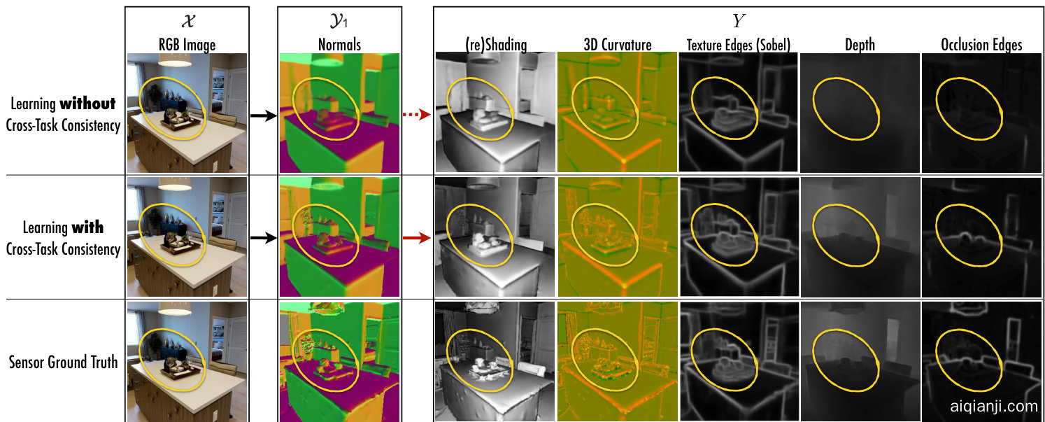
Figure 4: Learning with and without cross-task consistency shown for a sample query. Using the notation $x{\to}y_{1}{\to}Y$ , here ${\mathscr{X}}$ is RGB image, ${\textrm{y}{1}}$ is surface normals, and five domains in $Y$ are reshading, 3D curvature, texture edges (Sobel filter), depth, and occlusion edges. Top row shows the results of standard training of . After convergence of training, the predicted normals $(y_{1})$ are projected onto other domains $(Y)$ which reveals various inaccuracies. This demonstrates such cross-task projections $y_{1}\xrightarrow{}Y$ can provide additional cues to training ${\mathcal{X}}{\rightarrow}\mathcal{D}{1}$ . Middle row shows the results of consistent training of by leveraging $y_{1}\xrightarrow{}Y$ in the loss. The predicted normals are notably improved, especially in hard to predict fine-grained details (zoom into the yellow markers. Best seen on screen). Bottom row provides the ground truth. See video examples at visualization s webpage.
图 4: 展示样本查询中使用与未使用跨任务一致性的学习效果。采用符号$x{\to}y_{1}{\to}Y$表示,其中${\mathscr{X}}$为RGB图像,${\textrm{y}{1}}$为表面法线,$Y$中的五个域分别为重着色、3D曲率、纹理边缘(Sobel滤波器)、深度和遮挡边缘。首行显示标准训练的结果。训练收敛后,预测的法线$(y_{1})$被投影到其他域$(Y)$,暴露出多种不准确性。这表明跨任务投影$y_{1}\xrightarrow{}Y$能为训练${\mathcal{X}}{\rightarrow}\mathcal{D}{1}$提供额外线索。中间行显示通过损失函数利用$y_{1}\xrightarrow{}Y$实现一致性训练的结果,预测法线明显改善,尤其在难以预测的细粒度细节处(放大黄色标记处效果更佳)。末行为真实值。参见可视化网页中的视频示例。
This term $\mathcal{L}{\mathcal{X}\mathcal{Y}{1}\mathcal{Y}{2}}^{{p e r c e p t u a l}}$ no longer includes $y_{2}$ , hence it admits pair training data $(x,y_{1})$ rather than triplets $(x,y_{1},y_{2})$ . Comparing $\mathcal{L}{\mathcal{X}\mathcal{Y}{1}\mathcal{Y}{2}}^{{p e r c e p t u a l}}$ and $\mathcal{L}{\mathcal{X}\mathcal{Y}{1}\mathcal{Y}{2}}^{s e p a r a t e}$ shows the modification boiled down to replacing $y_{2}$ with $\tilde{f}{y_{1}y_{2}}(y_{1})$ . This makes intuitive sense too, as $y_{2}$ is the match of $y_{1}$ in the $y_{2}$ domain.
术语 $\mathcal{L}{\mathcal{X}\mathcal{Y}{1}\mathcal{Y}{2}}^{{p e r c e p t u a l}}$ 不再包含 $y_{2}$,因此它接受配对训练数据 $(x,y_{1})$ 而非三元组 $(x,y_{1},y_{2})$。比较 $\mathcal{L}{\mathcal{X}\mathcal{Y}{1}\mathcal{Y}{2}}^{{p e r c e p t u a l}}$ 和 $\mathcal{L}{\mathcal{X}\mathcal{Y}{1}\mathcal{Y}{2}}^{s e p a r a t e}$ 可以看出,修改的本质是用 $\tilde{f}{y_{1}y_{2}}(y_{1})$ 替换了 $y_{2}$。这也符合直观理解,因为 $y_{2}$ 是 $y_{1}$ 在 $y_{2}$ 域中的对应匹配。
Ill-posed tasks and imperfect networks: If $f_{y_{1}y_{2}}$ is a noisy estimator, then $f_{y_{1}y_{2}}(y_{1}){=}y_{2}{+}n o i s e$ rather than $f_{y_{1}y_{2}}(y_{1}){=}y_{2}$ . Using a noisy $f_{y_{1}y_{2}}$ in $\mathcal{L}{\mathcal{X}\mathcal{Y}{1}\mathcal{Y}{2}}^{s e p a r a t e}$ corrupts the training of $f_{\boldsymbol{\mathcal{X}}\boldsymbol{\mathcal{y}}{1}}$ since the second loss term does not reach 0 if $f_{x y_{1}}(x)$ correctly outputs $y_{1}$ . That is in contrast to $\mathcal{L}{\mathcal{X}\mathcal{Y}{1}\mathcal{Y}{2}}^{{p e r c e p t u a l}}$ where both terms have the same global minimum and are always 0 if $f_{x y_{1}}(x)$ outputs $y_{1}$ – even when $f_{y_{1}y_{2}}(y_{1}){=}y_{2}{+}n o i s e$ . This is crucial since neural networks are almost never perfect estimators, e.g. due to lacking an optimal training process for them or potential ill-posedness of the task $y_{1}\rightarrow y_{2}$ . Further discussion and experiments are available in supplementary material.
不适定任务与不完美网络:如果 $f_{y_{1}y_{2}}$ 是一个带噪声的估计器,则 $f_{y_{1}y_{2}}(y_{1}){=}y_{2}{+}n o i s e$ 而非 $f_{y_{1}y_{2}}(y_{1}){=}y_{2}$。在 $\mathcal{L}{\mathcal{X}\mathcal{Y}{1}\mathcal{Y}{2}}^{s e p a r a t e}$ 中使用带噪声的 $f_{y_{1}y_{2}}$ 会破坏 $f_{\boldsymbol{\mathcal{X}}\boldsymbol{\mathcal{y}}{1}}$ 的训练,因为当 $f_{x y_{1}}(x)$ 正确输出 $y_{1}$ 时,第二损失项不会归零。这与 $\mathcal{L}{\mathcal{X}\mathcal{Y}{1}\mathcal{Y}{2}}^{{p e r c e p t u a l}}$ 形成对比——后者两项具有相同的全局最小值,且当 $f_{x y_{1}}(x)$ 输出 $y_{1}$ 时总能归零(即使 $f_{y_{1}y_{2}}(y_{1}){=}y_{2}{+}n o i s e$)。这一特性至关重要,因为神经网络几乎不可能是完美估计器(例如由于训练过程未达最优,或任务 $y_{1}\rightarrow y_{2}$ 本身可能不适定)。补充材料提供了进一步讨论与实验。
Perceptual Loss: The process that led to Eq. 6 can be generally seen as using the loss $\left|g\circ f(x)-g(y)\right|$ instead of $\left|f(x)-y\right|$ . The latter compares $f(x)$ and $y$ in their explicit space, while the former compares them via the lens of function $g$ . This is often referred to as “perceptual loss” in superresolution and style transfer literature [19]–where two images are compared in the representation space of a network pretrained on ImageNet, rather than in pixel space. Similarly, the consistency constraint between the domains $y_{1}$ and $y_{2}$ in Eq. 6 (second term) can be viewed as judging the prediction $f_{x y_{1}}(x)$ against $y_{1}$ via the lens of the network $f_{y_{1}y_{2}}$ ; here $f_{y_{1}y_{2}}$ is a “perceptual loss” for training $f_{\boldsymbol{\mathcal{X}}\mathcal{y}{1}}$ . However, unlike the ImageNet-based perceptual loss [19], this function has the specific and interpret able job of enforcing consistency with another task. We also use multiple $f_{y_{1}y_{i}}\mathbf{s}$ simultaneously which enforces consistency of predicting $y_{1}$ against multiple other domains (Sections 3.2 and 3.3).
感知损失 (Perceptual Loss):推导出公式6的过程可以概括为使用损失函数$\left|g\circ f(x)-g(y)\right|$替代$\left|f(x)-y\right|$。后者在显式空间中直接比较$f(x)$和$y$,而前者通过函数$g$的视角进行比较。这种损失在超分辨率和风格迁移文献[19]中常被称为"感知损失"——此时两个图像是在ImageNet预训练网络的表征空间而非像素空间进行比较。类似地,公式6中域$y_{1}$和$y_{2}$间的一致性约束(第二项)可视为通过网络$f_{y_{1}y_{2}}$的视角来评判预测值$f_{x y_{1}}(x)$与$y_{1}$的匹配程度;此处$f_{y_{1}y_{2}}$就是用于训练$f_{\boldsymbol{\mathcal{X}}\mathcal{y}{1}}$的"感知损失"。但与基于ImageNet的感知损失[19]不同,该函数具有明确且可解释的职责——强制与其他任务保持一致性。我们还同时使用多个$f_{y_{1}y_{i}}\mathbf{s}$,通过多个其他域来强化$y_{1}$预测的一致性(见3.2和3.3节)。

Figure 5: Schematic summary of derived losses for $f_{\boldsymbol{\mathcal{X}}\mathscr{y}{1}}$ .(a): $\mathcal{L}{\mathcal{X}\mathcal{Y}{1}\mathcal{Y}{2}}^{t r i a n g l e}$ (Eq.1). (b): (Eq.3). (c): (Eq.6). (d): $\mathcal{L}{\mathcal{X Y}_{1}Y}^{p e r c e p t u a l}$ (Eq.7).
图 5: $f_{\boldsymbol{\mathcal{X}}\mathscr{y}{1}}$ 派生损失示意图。(a): $\mathcal{L}{\mathcal{X}\mathcal{Y}{1}\mathcal{Y}{2}}^{t r i a n g l e}$ (公式1)。(b): (公式3)。(c): (公式6)。(d): $\mathcal{L}{\mathcal{X Y}_{1}Y}^{p e r c e p t u a l}$ (公式7)。
3.2. Consistency of with ‘Multiple’ Domains
3.2. 与"多"领域的一致性
The derived $\mathcal{L}{\mathcal{X}\mathcal{Y}{1}\mathcal{Y}{2}}^{{p e r c e p t u a l}}$ loss augments learning of $f_{\boldsymbol{\mathcal{X}}\mathcal{y}{1}}$ with a consistency constraint against one domain $y_{2}$ . Straight forward extension of the same derivation to enforcing consistency of $f_{\boldsymbol{\mathcal{X}}\boldsymbol{\mathcal{y}}{1}}$ against multiple other domains (i.e. when $f_{\boldsymbol{\mathcal{X}}\boldsymbol{\mathcal{y}}_{1}}$ is part of multiple simultaneous triangles) yields:
推导出的 $\mathcal{L}{\mathcal{X}\mathcal{Y}{1}\mathcal{Y}{2}}^{{perceptual}}$ 损失通过针对一个域 $y_{2}$ 的一致性约束增强了 $f_{\boldsymbol{\mathcal{X}}\mathcal{y}{1}}$ 的学习。将相同推导直接扩展到强制 $f_{\boldsymbol{\mathcal{X}}\boldsymbol{\mathcal{y}}{1}}$ 对多个其他域的一致性(即当 $f_{\boldsymbol{\mathcal{X}}\boldsymbol{\mathcal{y}}_{1}}$ 是多个同时存在的三角形的一部分时)可得到:
$$
\mathcal{L}{\boldsymbol{x}\boldsymbol{y}{1}\boldsymbol{Y}}^{p e r c e p t u a l}\overset{\Delta}{=}|\boldsymbol{Y}|\times|f_{\boldsymbol{x}\boldsymbol{y}{1}}(\boldsymbol{x})-\boldsymbol{y}{1}|+\sum_{\boldsymbol{y}{i}\in\boldsymbol{Y}}|f_{\boldsymbol{y}{1}\boldsymbol{y}{i}}\circ f_{\boldsymbol{x}\boldsymbol{y}{1}}(\boldsymbol{x})-f_{\boldsymbol{y}{1}\boldsymbol{y}{i}}(\boldsymbol{y}_{1})|,
$$
$$
\mathcal{L}{\boldsymbol{x}\boldsymbol{y}{1}\boldsymbol{Y}}^{p e r c e p t u a l}\overset{\Delta}{=}|\boldsymbol{Y}|\times|f_{\boldsymbol{x}\boldsymbol{y}{1}}(\boldsymbol{x})-\boldsymbol{y}{1}|+\sum_{\boldsymbol{y}{i}\in\boldsymbol{Y}}|f_{\boldsymbol{y}{1}\boldsymbol{y}{i}}\circ f_{\boldsymbol{x}\boldsymbol{y}{1}}(\boldsymbol{x})-f_{\boldsymbol{y}{1}\boldsymbol{y}{i}}(\boldsymbol{y}_{1})|,
$$
where $Y$ is the set of domains with which $f_{\boldsymbol{\mathcal{X}}\boldsymbol{\mathcal{y}}{1}}$ must be consai sstpeencti, aal ncda $|Y|$ fi $\mathcal{L}{\mathcal{X}\mathcal{Y}{1}Y}^{p e r c e p t u a l}$ rd wi h near liet $Y{=}{y_{2}}$ $Y$ .o tFiicge. t5h satu $\mathcal{L}{\mathcal{X}\mathcal{Y}{1}\mathcal{Y}_{2}}^{{p e r c e p t u a l}}$ eiss the derivation of losses for fXY .
其中 $Y$ 是 $f_{\boldsymbol{\mathcal{X}}\boldsymbol{\mathcal{y}}{1}}$ 必须保持一致的域集合,且 $|Y|$ 当 $Y{=}{y_{2}}$ 时 $\mathcal{L}{\mathcal{X}\mathcal{Y}{1}Y}^{p e r c e p t u a l}$ 退化为 $\mathcal{L}{\mathcal{X}\mathcal{Y}{1}\mathcal{Y}_{2}}^{{p e r c e p t u a l}}$ ,这是针对 fXY 的损失函数推导。
Fig. 4 shows qualitative results of learning $f_{\boldsymbol{\mathcal{X}}\boldsymbol{\mathcal{y}}_{1}}$ with and without cross-task consistency for a sample query.
图 4: 展示了在有/无跨任务一致性的情况下,针对示例查询学习 $f_{\boldsymbol{\mathcal{X}}\boldsymbol{\mathcal{y}}_{1}}$ 的定性结果。
3.3. Beyond Triangles: Globally Consistent Graphs
3.3. 超越三角形:全局一致的图
The discussion so far has provided losses for the crosstask consistent training of one function $f_{\boldsymbol{\mathcal{X}}\boldsymbol{\mathcal{y}}{1}}$ with elementary triangle based units. We also assumed the functions $\mathcal{F}{y}$ were given apriori. The more general multi-task setup is: given a large set of domains, we are interested in learning functions that map the domains onto each other in a globally cross-task consistent manner. This objective can be formulated using a graph $\scriptstyle{\mathcal{G}}=({\mathcal{D}},{\mathcal{F}})$ with nodes representing all of the domains $\scriptstyle{\mathcal{D}}=(x\cup y)$ and edges being neural networks between them $\mathcal{F}{=}(\mathcal{F}{\mathcal{X}}\cup\mathcal{F}_{\mathcal{Y}})$ ; see Fig.2(c).
目前的讨论已为基于基本三角单元的函数 $f_{\boldsymbol{\mathcal{X}}\boldsymbol{\mathcal{y}}{1}}$ 的跨任务一致性训练提供了损失函数。我们还假设函数 $\mathcal{F}{y}$ 是预先给定的。更一般的多任务设置是:给定一个庞大的领域集合,我们希望学习能够以全局跨任务一致的方式将这些领域相互映射的函数。这一目标可以通过图 $\scriptstyle{\mathcal{G}}=({\mathcal{D}},{\mathcal{F}})$ 来表述,其中节点代表所有领域 $\scriptstyle{\mathcal{D}}=(x\cup y)$,边则是它们之间的神经网络 $\mathcal{F}{=}(\mathcal{F}{\mathcal{X}}\cup\mathcal{F}_{\mathcal{Y}})$;见图2(c)。
Extension to Arbitrary Paths: The transition from three domains to a large graph $\mathcal{G}$ enables forming more general consistency constraints using arbitrary-paths. That is, two paths with same endpoint should yield the same results – an example is shown in Fig.2(d). The triangle constraint in Fig.2(b,c) is a special and elementary case of the more general constraint in Fig.2(d), if paths with lengths 1 and 2 are picked for the green and blue paths. Extending the derivations done for a triangle in Sec. 3.1 to paths yields:
扩展到任意路径:从三个领域到大型图 $\mathcal{G}$ 的转变,使得我们能够利用任意路径形成更一般的约束条件。具体而言,两条具有相同终点的路径应当产生相同的结果——图2(d)展示了一个示例。若选择长度为1和2的路径分别作为绿色和蓝色路径,那么图2(b,c)中的三角约束实际上是图2(d)中更一般约束的特殊基础情形。将3.1节中对三角形的推导拓展到路径情形,可得到:
$$
\begin{array}{c}{{\mathcal{L}{\boldsymbol{x}\boldsymbol{y}{1}\boldsymbol{y}{2}...\boldsymbol{y}{k}}^{p e r e p t u a l}=|f_{\boldsymbol{x}\boldsymbol{y}{1}}(\boldsymbol{x})-\boldsymbol{y}{1}|+}}\ {{|f_{\boldsymbol{y}{k-1}\boldsymbol{y}{k}}\circ...\circ f_{\boldsymbol{y}{1}\boldsymbol{y}{2}}\circ f_{\boldsymbol{x}\boldsymbol{y}{1}}(\boldsymbol{x})-f_{\boldsymbol{y}{k-1}\boldsymbol{y}{k}}\circ...\circ f_{\boldsymbol{y}{1}\boldsymbol{y}{2}}(\boldsymbol{y}_{1})|,}}\end{array}
$$
$$
\begin{array}{c}{{\mathcal{L}{\boldsymbol{x}\boldsymbol{y}{1}\boldsymbol{y}{2}...\boldsymbol{y}{k}}^{p e r e p t u a l}=|f_{\boldsymbol{x}\boldsymbol{y}{1}}(\boldsymbol{x})-\boldsymbol{y}{1}|+}}\ {{|f_{\boldsymbol{y}{k-1}\boldsymbol{y}{k}}\circ...\circ f_{\boldsymbol{y}{1}\boldsymbol{y}{2}}\circ f_{\boldsymbol{x}\boldsymbol{y}{1}}(\boldsymbol{x})-f_{\boldsymbol{y}{k-1}\boldsymbol{y}{k}}\circ...\circ f_{\boldsymbol{y}{1}\boldsymbol{y}{2}}(\boldsymbol{y}_{1})|,}}\end{array}
$$
which is the loss for training $f_{\boldsymbol{\mathcal{X}}\boldsymbol{\mathcal{y}}{1}}$ using the arbitrary consistency path $\mathcal{X}{\rightarrow}\mathcal{Y}{1}{\rightarrow}\mathcal{Y}{2}{\leftarrow}{\rightarrow}\mathcal{Y}{k}$ with length $k$ (full derivation provided in supplementary material). Notice that Eq. 6 is a special case of Eq. 8 if $k{=}2$ . Equation 8 is particularly useful for incomplete graphs; if the function $y_{1}\rightarrow y_{k}$ is missing, consistency between domains $y_{1}$ and $y_{k}$ can still be enforced via transitivity through other domains using Eq. 8.
这是用于训练 $f_{\boldsymbol{\mathcal{X}}\boldsymbol{\mathcal{y}}{1}}$ 的损失函数,其中使用了长度为 $k$ 的任意一致性路径 $\mathcal{X}{\rightarrow}\mathcal{Y}{1}{\rightarrow}\mathcal{Y}{2}{\leftarrow}{\rightarrow}\mathcal{Y}{k}$(完整推导见补充材料)。值得注意的是,当 $k{=}2$ 时,式(6) 是式(8) 的特例。式(8) 对于不完整图特别有用:如果函数 $y_{1}\rightarrow y_{k}$ 缺失,仍然可以通过式(8) 借助其他域的传递性来强制实现域 $y_{1}$ 和 $y_{k}$ 之间的一致性。
Also, extending Eq. 8 to multiple simultaneous paths (as in Eq. 7) by summing the path constraints is straightforward.
此外,通过对路径约束求和,将方程8扩展到多条同时存在的路径(如方程7所示)是直接可行的。
Global Consistency Objective: We define reaching global cross-task consistency for graph $\mathcal{G}$ as satisfying the consistency constraint for all feasible paths in $\mathcal{G}$ . We can write the global consistency objective for $\mathcal{G}$ as $\mathcal{L}{\mathcal{G}}=$ $\textstyle\sum_{p\in{\mathcal{P}}}\mathcal{L}_{p}^{p e r c e p t u a l}$ , where $p$ represents a path and $\mathcal{P}$ is the set of all feasible paths in $\mathcal{G}$ .
全局一致性目标:我们定义图 $\mathcal{G}$ 达到全局跨任务一致性为满足 $\mathcal{G}$ 中所有可行路径的一致性约束。可以将 $\mathcal{G}$ 的全局一致性目标表示为 $\mathcal{L}{\mathcal{G}}=$ $\textstyle\sum_{p\in{\mathcal{P}}}\mathcal{L}_{p}^{perceptual}$,其中 $p$ 表示路径,$\mathcal{P}$ 是 $\mathcal{G}$ 中所有可行路径的集合。
Optimizing the objective $\mathcal{L}{\mathcal{G}}$ directly is intractable as it would require simultaneous training of all networks in $\mathcal{F}$ with a massive number of consistency paths7. In Alg.1 we devise a straightforward training schedule for an approximate optimization of $\mathcal{L}_{\mathcal{G}}$ . This problem is similar to inference in graphical models, where one is interested in marginal distribution of unobserved nodes given some observed nodes by passing “messages” between them through the graph until convergence. As exact inference is usually intractable for un constrained graphs, often an approximate message passing algorithm with various heuristics is used.
直接优化目标函数 $\mathcal{L}{\mathcal{G}}$ 是不可行的,因为这需要同时训练 $\mathcal{F}$ 中所有网络并处理海量一致性路径7。在算法1中,我们设计了一种简单的训练方案来近似优化 $\mathcal{L}_{\mathcal{G}}$。该问题类似于图模型中的推理过程,即通过节点间传递"消息"直至收敛,从而根据已观测节点推断未观测节点的边缘分布。由于无约束图结构通常难以进行精确推理,实践中常采用启发式近似消息传递算法。
Algorithm 1 selects one network $f_{i j}\in\mathcal{F}$ to be trained, selects consistency path(s) $p{\in}\mathcal{P}$ for it, and trains $f_{i j}$ with $p$ for a fixed number of steps using loss 8 (or its multi path version if multiple paths selected). This is repeated until all networks in $\mathcal{F}$ satisfy a convergence criterion.
算法 1 选择一个待训练的网络 $f_{i j}\in\mathcal{F}$ ,为其选择一致性路径 $p{\in}\mathcal{P}$ ,并使用损失函数 8 (若选择多路径则采用其多路径版本) 对 $f_{i j}$ 进行固定步数的训练。该过程重复执行,直至 $\mathcal{F}$ 中所有网络均满足收敛条件。
A number of choices for the selection criterion in SelectNetwork and SelectPath is possible, including round-robin and random selection. While we did not observe a significant difference in the final results, we achieved the best results using maximal violation criterion: at each step select the network and path with the largest loss8. Also, Alg.1 starts from shorter paths and progressively opens up to longer ones (up to length $L$ ) only after shorter paths have converged. This is based on the observation that the value of short and long paths in terms of enforcing cross-task consistency overlap, while shorter paths are computationally cheaper8. For the same reason, all of the networks are initialized by training using the standard direct loss (Op.1 in Alg.1) before progressively adding consistency terms.
在SelectNetwork和SelectPath中选择标准有多种可能,包括轮询和随机选择。虽然我们未观察到最终结果的显著差异,但采用最大违反准则时获得了最佳效果:每一步选择损失最大的网络和路径[8]。此外,算法1从较短路径开始,仅在短路径收敛后逐步扩展至较长路径(最大长度$L$)。这一设计基于以下观察:短路径与长路径在实现跨任务一致性方面的价值存在重叠,而短路径的计算成本更低[8]。出于相同原因,所有网络在逐步添加一致性项之前,都先通过标准直接损失(算法1中的操作1)进行初始化训练。
Algorithm 1: Globally Cross-Task Consistent Learning of Networks $\mathcal{F}$
算法 1: 网络的全局跨任务一致性学习 $\mathcal{F}$
| 结果: 训练图G的边F | |
|---|---|
| 1 | 独立训练每个f∈F → 通过标准直接训练初始化。 |
| 2 | for k←2 to L do |
| 3 | while 损失未收敛(F) do |
| 4 | fi←选择网络(F) 选择待训练的目标网络。 |
| 5 | p←选择路径(fi,j,k,P) 从P中为fi,j选择最大长度为k的可行一致性路径。 |
| 6 | 优化 C感知损失 ijp > 使用路径约束p在损失函数8中训练fi。 |
| 7 | end |
| 8 | end |
Finally, Alg.1 does not distinguish between ${\mathcal{F}}{x}$ and ${\mathcal{F}}{x}$ and can be used to train them all in the same pool. This means the selected path $p$ may include networks not fully converged yet. This is not an issue in practice, because, first, all networks are pre-trained with their direct loss (Op.1 in Alg.1) thus they are not wildly far from their convergence point. Second, the perceptual loss formulation makes training $f_{i j}$ robust to imperfections in functions in $p$ (Sec. 3.1.2). However, as practical applications primarily care about ${\mathcal{F}}{x}$ , rather than $\mathcal{F}{y}$ , one can first train $\mathcal{F}{y}$ to convergence using Alg.1, then start the training of ${\mathcal{F}}{x}$ with well trained and converged networks $\mathcal{F}_{y}$ . We do the latter in our experiments.
最后,算法1并未区分 ${\mathcal{F}}{x}$ 和 ${\mathcal{F}}{x}$ ,可以在同一池中训练所有网络。这意味着所选路径 $p$ 可能包含尚未完全收敛的网络。但这在实际应用中不成问题,因为首先所有网络都通过其直接损失进行了预训练(算法1中的操作1),因此距离收敛点并不遥远。其次,感知损失的公式设计使得训练 $f_{i j}$ 对路径 $p$ 中函数的不完美具有鲁棒性(第3.1.2节)。然而,由于实际应用主要关注 ${\mathcal{F}}{x}$ 而非 $\mathcal{F}{y}$ ,可以先使用算法1将 $\mathcal{F}{y}$ 训练至收敛,再用训练好的收敛网络 $\mathcal{F}{y}$ 启动 ${\mathcal{F}}_{x}$ 的训练。我们在实验中采用了后一种方法。
Please see supplementary material for how to normalize and balance the direct and consistency loss terms, as they belong to different domains with distinct numerical properties.
请参阅补充材料了解如何对直接损失和一致性损失项进行归一化和平衡,因为它们属于具有不同数值属性的不同领域。
4. Consistency Energy
4. 一致性能量
We quantify the amount of cross-task consistency in the system using an energy-based quantity [26] called Consistency Energy. For a single query $x$ and domain $_{\mathcal{V}k}$ , the consistency energy is defined to be the standardized average of pairwise inconsistencies:
我们使用基于能量的指标[26]——一致性能量(Consistency Energy)来量化系统中的跨任务一致性程度。对于单个查询$x$和领域$_{\mathcal{V}k}$,一致性能量定义为两两不一致性的标准化平均值:
$$
\operatorname{Energy}{\mathcal{D}{k}}(x)\triangleq\frac{1}{|y|-1}\sum_{\begin{array}{l}{y_{i}\in y,i\neq k}\end{array}}\frac{|f_{y_{i}y_{k}}\circ f_{\mathcal{X}\mathcal{Y}{i}}(x)-f_{\mathcal{X}\mathcal{Y}{k}}(x)|-\mu_{i}}{\sigma_{i}},
$$
$$
\operatorname{Energy}{\mathcal{D}{k}}(x)\triangleq\frac{1}{|y|-1}\sum_{\begin{array}{l}{y_{i}\in y,i\neq k}\end{array}}\frac{|f_{y_{i}y_{k}}\circ f_{\mathcal{X}\mathcal{Y}{i}}(x)-f_{\mathcal{X}\mathcal{Y}{k}}(x)|-\mu_{i}}{\sigma_{i}},
$$
where $\mu_{i}$ and $\sigma_{i}$ are the average and standard deviation of $\vert f_{y_{i}y_{k}}\circ f_{x y_{i}}(x)-f_{x y_{k}}(x)\vert$ over the dataset. Eq. 9 can be computed per-pixel or per-image by average over its pixels. Intuitively, the energy can be thought of as the amount of variance in predictions in the lower row of Fig. 3 – the higher the variance, the higher the inconsistency, and the higher the energy. The consistency energy is an intrinsic quantity of the system and needs no ground truth or supervision.
其中 $\mu_{i}$ 和 $\sigma_{i}$ 分别是数据集上 $\vert f_{y_{i}y_{k}}\circ f_{x y_{i}}(x)-f_{x y_{k}}(x)\vert$ 的平均值和标准差。公式9可以逐像素计算,也可以通过像素平均实现逐图像计算。直观上,该能量可理解为图3下方行中预测结果的方差大小——方差越大,不一致性越高,能量值也越大。这种一致性能量是系统的固有属性,无需真实标签或监督信号。

Figure 6: Qualitative results of predicting multiple domains along with the pixel-wise Consistency Energy. The top queries are from the Taskonomy dataset’s test set. The results of networks trained with consistency are more accurate, especially in fine-grained regions (zoom into the yellow markers), and more correlated across different tasks. The bottom images are external queries (no ground truth available) demonstrating the generalization and robustness of consistency networks to external data. Comparing the energy against a prediction domain (e.g. normals) shows that energy often correlates with error. More examples are provided in the project page, and a live demo for user uploaded images is available at the demo page. External Queries: Bedroom in Arles, Van Gogh (1888); Cotton Mill Girl, Lewis Hine (1908); Chernobyl Pripyat Abandoned School (c. 2009). [best seen on screen]
图 6: 多领域预测结果及像素级一致性能量(Consistency Energy)可视化。顶部查询样本来自Taskonomy数据集的测试集,经过一致性训练的网络预测结果更精确(尤其关注黄色标记处的细粒度区域),且跨任务相关性更强。底部为外部查询样本(无真实标注数据),展示了一致性网络对外部数据的泛化性与鲁棒性。将能量值与预测域(如法线图)对比可见,能量值常与误差呈正相关。更多案例详见项目页面,用户上传图像的实时演示可访问演示页面。外部查询样本: 梵高《阿尔勒的卧室》(1888);路易斯·海因《棉纺厂女孩》(1908);切尔诺贝利普里皮亚季废弃学校(约2009年)。[建议屏幕查看]
In Sec. 5.3, we show this quantity turns out to be quite informative as it can indicate the reliability of predictions (useful as a confidence/uncertainty metric) or a shift in the input domain (useful for domain adaptation). This is based on the fact that if the query is from the same data distribution as the training and is un challenging, all inference paths of a system trained with consistency path constraints work well and yield similar results (as they were trained to); whereas under a distribution shift or for a challenging query, different paths break in different ways resulting in dissimilar predictions. In other words, usually correct predictions are consistent while mistakes are inconsistent. (Plots 9(b), 9(c), 9(d).)
在5.3节中,我们证明该指标具有重要参考价值,因为它既能反映预测的可靠性(可作为置信度/不确定性度量),又能检测输入域的分布变化(适用于域适应场景)。其原理在于:若查询样本与训练数据同分布且难度较低,受一致性路径约束训练的系统所有推理路径都会表现良好且结果相近(符合训练目标);而当出现分布偏移或困难查询时,不同路径会以不同方式失效,导致预测结果出现分歧。换言之,正确预测通常保持一致,而错误预测往往相互矛盾(见绘图9(b)、9(c)、9(d))。
5. Experiments
5. 实验
The evaluations are organized to demonstrate the proposed approach yields predictions that are I. more consistent (Sec.5.1), II. more accurate (Sec.5.2), and III. more generalizable to out-of-training-distribution data (Sec.5.4). We also IV. quantitatively analyze the Consistency Energy and report its utilities (Sec.5.3).
评估旨在证明所提出的方法能够产生以下预测结果:I. 更一致(第5.1节),II. 更准确(第5.2节),以及III. 对训练分布外数据更具泛化性(第5.4节)。此外,我们还IV. 定量分析了Consistency Energy(一致性能量)并报告了其效用(第5.3节)。
Datasets: We used the following datasets in the evaluations:
数据集:我们在评估中使用了以下数据集:
Taskonomy [45]: We adopted Taskonomy as our main training dataset. It includes 4 million real images of indoor scenes with multi-task annotations for each image. The experiments were performed using the following 10 domains from the dataset: RGB images, surface normals, principal curvature, depth (zbuffer), reshading, 3D (occlusion) edges, 2D (Sobel) texture edges, 3D keypoints, 2D keypoints, semantic segmentation. The tasks were selected to cover 2D, 3D, and semantic domains and have sensorbased/semantic ground truth. We report results on the test set.
Taskonomy [45]: 我们采用Taskonomy作为主要训练数据集。该数据集包含400万张室内场景的真实图像,每张图像都带有多任务标注。实验使用了数据集中的以下10个领域:RGB图像、表面法线、主曲率、深度(zbuffer)、重着色、3D(遮挡)边缘、2D(Sobel)纹理边缘、3D关键点、2D关键点、语义分割。这些任务的选择覆盖了2D、3D和语义领域,并具有基于传感器/语义的真实值。我们在测试集上报告结果。
Replica[40] has high resolution 3D ground truth and enables more reliable evaluations of fine-grained details. We test on 1227 images from Replica (no training), besides Taskonomy test data.
Replica[40] 拥有高分辨率3D真实数据,能更可靠地评估细粒度细节。除Taskonomy测试数据外,我们还在Replica的1227张图像上进行了测试(无训练)。
CocoDoom [27] contains synthetic images from the Doom video game. We use it as one of the out-of-training-distribution datasets.
CocoDoom [27] 包含来自《毁灭战士》(Doom)电子游戏的合成图像。我们将其用作训练分布外数据集之一。
NYU [37]: We also evaluated on NYUv2. The findings are similar to those on Taskonomy and Replica (in supplementary material).
NYU [37]: 我们也在NYUv2数据集上进行了评估。结果与Taskonomy和Replica数据集上的发现类似 (详见补充材料)。
Architecture & Training Details: We used a UNet [34] backbone architecture. All networks in ${\mathcal{F}}{\mathcal{X}}$ and $\mathcal{F}{y}$ have a similar architecture. The networks have 6 down and 6 up sampling blocks and were trained using AMSGrad [33] and Group Norm [42] with learning rate $3\times10^{-5}$ , weight decay $2\times10^{-6}$ , and batch size 32. Input and output images were linearly scaled to the range [0, 1] and resized down to $256\times256$ . We used $\ell_{1}$ as the norm in all losses and set the max path length $L{=}3$ .
架构与训练细节:我们采用了UNet [34]作为主干架构。${\mathcal{F}}{\mathcal{X}}$和$\mathcal{F}{y}$中的所有网络均采用相似架构。网络包含6个下采样和6个上采样模块,训练时使用AMSGrad [33]和Group Norm [42]优化器,学习率为$3\times10^{-5}$,权重衰减为$2\times10^{-6}$,批量大小为32。输入输出图像线性缩放至[0, 1]范围并下采样至$256\times256$分辨率。所有损失函数采用$\ell_{1}$范数,最大路径长度设为$L{=}3$。
Baselines: The main baseline categories are described below. To prevent confounding factors, our method and all baselines were implemented using the same UNet network when feasible and were re-trained on Taskonomy dataset.
基线方法:主要基线类别如下所述。为避免混淆因素,在可行情况下,我们采用相同的UNet网络实现本文方法与所有基线方法,并在Taskonomy数据集上重新训练。
Baseline UNet (standard independent learning) is the main baseline. It is identical to consistency models in all senses, except being trained with only the direct loss and no consistency terms.
基线 UNet (标准独立学习) 是主要基线。除仅使用直接损失训练且不含一致性项外,其在所有方面都与一致性模型相同。
Multi-task learning: A network with one shared encoder and multiple decoders each dedicated to a task, similar to [21].
多任务学习:一个共享编码器和多个解码器组成的网络,每个解码器专用于一项任务,类似于 [21]。
Cycle-based consistency, e.g.[50], is a way of enforcing consistency requiring a bijection between domains. This baseline is the special case of the triangle in Fig.2(b) by setting $f_{\mathcal{X Y}_{2}}{=}i d e n t i t y$ .
基于循环的一致性 (cycle-based consistency) ,例如 [50],是一种通过要求域间双射来强制实现一致性的方法。该基线是图 2(b) 中三角形的特例,通过设置 $f_{\mathcal{X Y}_{2}}{=}i d e n t i t y$ 实现。
Baseline perceptual loss network uses frozen random (Gaussian weight) networks as $\mathcal{F}_{y}$ , rather than training them to be crosstask functions. This baseline would show if the improvements were owed to the priors in the architecture of constraint networks, rather than them executing cross-task consistency constraints.
基线感知损失网络使用冻结的随机(高斯权重)网络作为$\mathcal{F}_{y}$,而非将其训练为跨任务函数。该基线用于验证改进是否源于约束网络架构中的先验,而非执行跨任务一致性约束。
GAN-based image translation: We used Pix2Pix [17].
基于GAN的图像翻译:我们使用了Pix2Pix [17]。
Blind guess:A query-agnostic statistically informed guess computed from data for each domain (visuls in supplementary). It shows what can be learned from general dataset regularities. [45]
盲猜:一种基于数据计算的、与查询无关的统计预测(可视化见补充材料),展示了从通用数据集规律中可学习的内容。[45]

Figure 7: Learning with cross-task consistency vs various baselines compared over surface normals. Queries are from Taskonomy dataset (top) or external data (bottom). More examples are provided in project page, and a live demo for user uploaded images is available at demo page. [best seen on screen]
图 7: 跨任务一致性学习与各种基线方法在表面法线预测任务上的对比。查询图像来自Taskonomy数据集(上)或外部数据(下)。更多示例详见项目页面,用户上传图像的实时演示可访问演示页面。[建议屏幕观看]
Table 1: Quantitative Evaluation of Cross-Task Consistent Learning vs Baselines. Results are reported on Replica and Taskonomy Datasets for four prediction tasks (normals, depth, reshading, pixel-wise semantic labeling) using ‘Direct’ and ‘Perceptual’ error metrics. The Perceptual metrics evaluate the target prediction in another domain (e.g., the leftmost column evaluates the depth inferred out of the predicted normals). Bold marks the best-performing method. If more than one value is bold, their performances were statistically indistinguishable from the best, according to 2-sample paired t-test $\alpha=0.01$ . Learning with consistency led to improvements with large margins in most columns. (In all tables, $\ell$ norm values are multiplied by 100 for readability. Methods that cannot be run for a given target are denoted by $\ '\times:$ )
表 1: 跨任务一致性学习与基线的定量评估。结果在Replica和Taskonomy数据集上针对四种预测任务(法线、深度、重着色、像素级语义标注)使用"直接"和"感知"误差指标进行报告。感知指标评估另一领域的目标预测(例如最左列评估从预测法线推断的深度)。加粗表示性能最佳的方法。若多个值加粗,则根据双样本配对t检验(α=0.01)其性能与最佳方法无统计学差异。一致性学习在大多数列中带来了显著提升。(所有表格中,ℓ范数值乘以100以便阅读。无法运行给定目标的方法标记为×)
| 方法 | 感知误差 | 法线 | 直接 | Replica数据集深度 | 重着色 | 深度 | Taskonomy数据集 | 重着色 | 语义分割 | |||||||||||||||||||||||||||||
|---|---|---|---|---|---|---|---|---|---|---|---|---|---|---|---|---|---|---|---|---|---|---|---|---|---|---|---|---|---|---|---|---|---|---|---|---|---|---|
| 深度 重着色 | e1 | 误差 | 法线 重着色 | e1 | 误差 | 法线 深度 | 误差 | 深度 重着色 曲率.边缘(2D) | 误差 | 法线.重着色 曲率. 边缘(2D) | 误差 | 法线.深度 曲率.边缘(2D) | 误差 | |||||||||||||||||||||||||
| 随机猜测 | 4.75 | 33.31 | 16.02 | 22.23 | 19.94 | 4.81 | 15.74 | 5.14 | 16.45 | 7.39 | 38.11 | 3.91 | 12.05 | 17.77 | 22.37 | 27.27 | 7.96 | 12.77 | 7.07 | 19.96 | 7.14 | 3.53 | 12.62 | 24.85 | ||||||||||||||
| Taskonomy网络 | 3.73 | 11.07 | 6.55 | 18.06 | 15.39 | 3.72 | 8.70 | 3.85 | 11.43 | 7.19 | 22.68 | 3.68 | 10.70 | 7.54 | 18.82 | 20.83 | 6.65 | 14.10 | 4.55 | 11.72 | 4.69 | 3.54 | 11.19 | |||||||||||||||
| 多任务 | 5.58 | 22.11 | 6.03 7.48 | 15.30 13.88 | 16.14 14.03 | 2.44 4.01 | 7.24 | × | 3.36 × | 10.32 | 8.78 7.71 | 27.32 | 3.65 | 10.16 | 7.07 | 17.18 | 19.55 | 7.54 | 13.67 | 2.81 | 9.19 | 3.54 | 3.56 | |||||||||||||||
| GeoNet(原版)循环一致性 | 6.23 | 19.34 22.39 | 7.13 | × | 27.35 30.33 | 3.32 3.84 | 9.09 10.26 | 9.58 8.68 | 15.44 | 18.73 | 4.03 | 10.78 | 4.07 | × | × | |||||||||||||||||||||||
| 基线感知损失 | 5.65 4.88 | 15.34 | 4.99 | 8.59 | 23.98 | 3.41 | 10.01 | 6.17 | ||||||||||||||||||||||||||||||
| Pix2Pix | 4.52 | 19.03 | 13.15 | 7.70 4.96 | 10.47 | 12.99 | 1.99 | 6.90 | 2.74 | 9.55 | 8.12 8.17 | 26.23 20.94 | 3.83 | 10.33 | 5.95 | 9.40 | ||||||||||||||||||||||
| 基线UNet(e) GeoNet(更新) | 4.69 | 4.62 | 12.79 | 4.70 | 10.47 | 12.75 | 1.83 | 8.18 | 20.84 | 3.40 | 9.99 | 5.91 | 13.77 | 15.76 | 7.52 | 12.61 12.67 | 2.27 2.26 | 9.58 | × | |||||||||||||||||||
| X-任务一致性 0.25%数据:基线 | 2.07 | 9.99 | 4.80 7.61 | 7.01 | 4.32 | 12.15 |
GeoNet [32] is a task-specific consistency method analytically curated for depth and normals. This baseline shows how closely the task-specific consistency methods based on known analytical relationships perform vs the proposed generic data-driven method. The “original” and “updated” variants represent original authors’ released networks and our re-implemented and re-trained version.
GeoNet [32] 是一种针对深度和法线任务专门设计的一致性分析方法。该基线展示了基于已知解析关系的任务专用一致性方法与所提出的通用数据驱动方法之间的性能差距。"original"和"updated"变体分别代表原作者发布的网络版本与我们重新实现并训练的版本。
5.1. Consistency of Predictions
5.1. 预测一致性
Fig.9(a) (blue) shows the amount of inconsistency in test set predictions (Consistency Energy) successfully decreases over the course of training. The convergence point of the network trained with consistency is well below baseline independent learning (orange) and multi-task learning (green)– which shows consistency among predictions does not naturally emerge in either case without explicit constraining.
图 9(a) (蓝色) 显示了测试集预测中的不一致性量(Consistency Energy)在训练过程中成功降低。采用一致性训练的网络的收敛点明显低于基线独立学习(橙色)和多任务学习(绿色) - 这表明在缺乏显式约束的情况下,预测间的一致性不会自然形成。
5.2. Accuracy of Predictions
5.2. 预测准确性
Figures 6 and 7 compare the prediction results of networks trained with cross-task consistency against the baselines in different domains. The improvements are considerable particularly around the difficult fine-grained details.
图 6 和图 7 对比了采用跨任务一致性训练的网络与各领域基线的预测结果。在难以处理的细粒度细节区域,改进效果尤为显著。
Quantitative evaluations are provided in Tab. 1 for Replica dataset and Taskonomy datasets on depth, normal, reshading, and pixel-wise semantic prediction tasks. Learning with consistency led to large improvements in most of the setups. As most of the pixels in an image belong to easy to predict regions governed by the room layout (e.g. ceiling, walls), the standard pixel-wise error metrics (e.g. $\ell_{1}$ ) are dominated by them and consequently insensitive to fine-grained changes. Thus, besides standard Direct metrics, we report Perceptual error metric (e.g. normal $\rightarrow$ curvature) that evaluate the same prediction, but with a non-uniform attention to pixel properties.9 Each perceptual error provides a different angle, and the optimal results would have a low error for all metrics.
定量评估结果如表 1 所示,涵盖了 Replica 数据集和 Taskonomy 数据集在深度、法线、重着色和像素级语义预测任务上的表现。采用一致性学习的方法在大多数实验设置中都取得了显著提升。由于图像中大部分像素属于易于预测的房间布局区域(如天花板、墙壁),标准像素级误差指标(如 $\ell_{1}$ )会受其主导,因此对细粒度变化不敏感。为此,除标准直接指标外,我们还报告了感知误差指标(如法线 $\rightarrow$ 曲率),这些指标通过非均匀关注像素属性来评估相同预测结果。每种感知误差都提供了不同视角,最优结果应使所有指标均保持较低误差。
Tab. 1 also includes evaluation of the networks when trained with little data $0.25%$ subset of Taskonomy dataset), which shows the consistency constraints are useful under low-data regime as well.
表 1 还包含了网络在少量数据 (Taskonomy 数据集的 0.25% 子集) 训练时的评估结果,这表明一致性约束在低数据量情况下同样有效。
We adopted normals as the canonical task for more extensive evaluations, due to its practical value and abundance of baselines. The conclusions remained the same regardless.
我们选择法线贴图作为标准任务进行更广泛的评估,因其具有实用价值和丰富的基线数据。无论采用何种方法,结论均保持一致。
5.3. Utilities of Consistency Energy
5.3. 一致性能量的效用
Below we quantitatively analyze the Consistency Energy. The energy is shown (per-pixel) for sample queries in Fig. 6.
下面我们定量分析一致性能量 (Consistency Energy)。图6展示了示例查询的(每像素)能量值。
Consistency Energy as a Confidence Metric: The plot 9(b) shows the energy of predictions has a strong positive correlation with the error computed using ground truth (Pearson corr. 0.67). This suggests the energy can be adopted for confidence quant if i cation and handling uncertainty. This experiment was done on Taskonomy test set.
一致性能量作为置信度指标:图 9(b) 显示预测能量与基于真实值计算的误差呈强正相关性 (Pearson 相关系数 0.67)。这表明该能量可用于置信度量化 (confidence quantification) 和不确定性处理。本实验在 Taskonomy 测试集上完成。

Figure 8: Error with Increasing (Smooth) Domain Shift. The network trained with consistency is more robust to the shift.
图 8: 随着(平滑)域偏移增加的误差。使用一致性训练的网络对偏移更具鲁棒性。
| NovelDomain | Error(Post-Adaption) | Error (Pre-Adaptation) | |||
|---|---|---|---|---|---|
| #images | Consistency | Baseline | Consistency | Baseline | |
| Gaussianblur | 128 | 17.4 (+14.7%) | 20.4 | 46.2 (+12.8%) | 53.0 |
| (Taskonomy) | 16 | 22.3(+8.6%) | 24.4 | ||
| CocoDoom | 128 | 18.5 (+19.2%) | 22.9 | 54.3 (+15.8%) | 64.5 |
| 16 | 27.1 (+24.5%) | 35.9 | |||
| ApolloScape | 8 | 40.5 (+11.9%) | 46.0 | 55.8(+5.5%) | 59.1 |

Table 2: Domain generalization and adaptation on CocoDoom, ApolloS cape, and Taskonomy blur data. Networks trained with consistency show better generalization to new domains and a faster adaptation with little data. (relative improvement in parentheses) (c)Energy vs Discrete Domain Shift (d) Energy vs Continuous Domain Shift Figure 9: Analyses of Consistency Energy.
表 2: CocoDoom、ApolloS cape 和 Taskonomy 模糊数据上的领域泛化与适应表现。通过一致性训练的模型在新领域展现出更好的泛化能力,并能用少量数据快速适应 (括号内为相对提升百分比)。
(c) 能量与离散领域偏移的关系
(d) 能量与连续领域偏移的关系
图 9: 一致性能量分析。
Consistency Energy as a Domain Shift Detector: Plot 9(c) shows the energy distribution of in-distribution (Taskonomy) and out-of-distribution datasets (ApolloS cape, CocoDoom). Out-of-distribution datapoints have notably higher energy values, which suggests that energy can be used to detect anomalous samples or domain shifts. Using the per-image energy value to detect out-of-distribution images achieved ROC-AUC $=0.95$ ; the out-of-distribution detection method OC-NN [3] scored 0.51.
一致性能量作为域偏移检测器:图9(c)展示了分布内(Taskonomy)和分布外数据集(ApolloS cape, CocoDoom)的能量分布。分布外数据点具有显著更高的能量值,这表明能量可用于检测异常样本或域偏移。使用单图像能量值检测分布外图像实现了ROC-AUC $=0.95$;而分布外检测方法OC-NN [3]得分为0.51。
Plot 9(d) shows the same concept as 9(c) (energy vs domain shift), but when the shift away from the training data is smooth. The shift was done by applying a progressively stronger Gaussian blur with kernel size 6 on Taskonomy test images. The plot also shows the error computed using ground truth which has a pattern similar to the energy.
图 9(d) 展示了与 9(c) 相同的概念 (能量与域偏移的关系),但此时训练数据的偏移是平滑的。这种偏移是通过在 Taskonomy 测试图像上逐步应用更强的高斯模糊 (kernel size 6) 实现的。图中还显示了使用真实值计算的误差,其模式与能量相似。
We find the reported utilities noteworthy as handling uncertainty, domains shifts, and measuring prediction confidence in neutral networks are open topics of research [29, 11] with critical values in, e.g. active learning [35], real-world decision making [20], and robotics [31].
我们发现所报告的效用值得关注,因为处理不确定性、领域偏移以及测量中性网络中的预测置信度仍是开放的研究课题 [29, 11],这些课题在主动学习 [35]、现实世界决策 [20] 和机器人技术 [31] 等领域具有关键价值。
5.4. Generalization & Adaptation to New Domains
5.4. 泛化与新领域适应
To study: I. how well the networks generalize to new domains without any adaptation and quantify their resilience, and II. how efficiently they can adapt to a new domain given a few training examples by fine-tuning, we test the networks trained on Taskonomy dataset on various new domains.
研究目标:
I. 评估网络在未经任何适配的情况下对新领域的泛化能力,并量化其鲁棒性;
II. 通过微调少量训练样本,衡量网络高效适应新领域的能力。为此,我们在多个新领域上测试了基于Taskonomy数据集训练的网络。
In interest of space, we defer the details to the supplementary and provide the results in Fig. 8 and Tab. 2. Networks trained with consistency generally show higher resilience w.r.t. domain shifts and better adaptation with little data.
为节省篇幅,我们将细节内容移至补充材料,并在图8和表2中展示结果。采用一致性训练的模型通常对领域偏移表现出更强的鲁棒性,且能以少量数据实现更好的适应效果。
Supplementary Material: We defer additional discussions and experiments, particularly analyzing different aspects of the optimization, stability analysis of the experimental trends, and proving qualitative results at scale to the supplementary material and the project page.
补充材料:我们将额外讨论和实验(特别是优化不同方面的分析、实验趋势的稳定性分析以及大规模定性结果的验证)推迟到补充材料和项目页面中。
6. Conclusion and Limitations
6. 结论与局限性
We presented a general and data-driven framework for augmenting standard learning with cross-task consistency. The evaluations showed learning with cross-task consistency fits the data better yielding more accurate predictions and leads to models with improved generalization. The Consistency Energy was found to be an informative intrinsic quantity with utilities toward confidence estimation and domain shift detection. We briefly discuss some of the limitations:
我们提出了一种通用的数据驱动框架,通过跨任务一致性来增强标准学习。评估表明,采用跨任务一致性的学习能更好地拟合数据,从而产生更准确的预测,并提升模型的泛化能力。研究发现,一致性能量 (Consistency Energy) 是一种具有信息量的内在指标,可用于置信度估计和域偏移检测。我们简要讨论了一些局限性:
Path Ensembles: we used the various inference paths only as a way of enforcing consistency. Aggregation of multiple (comparably weak) inference paths into a single strong estimator (e.g. in a manner similar to boosting) is a promising direction that this paper did not address.
路径集成:我们仅将各种推理路径用作确保一致性的手段。将多个(相对较弱的)推理路径聚合为单个强估计器(例如以类似提升(boosting)的方式)是本文未涉及的一个有前景的方向。
Categorical/Low-Dimensional Tasks: We primarily exper- imented with pixel-wise tasks. Classification tasks, and generally tasks with low-dimensional outputs, will be interested to experiment with, especially given the more severely ill-posed cross-task relationships they induce.
分类/低维任务:我们主要尝试了像素级任务。分类任务及通常具有低维输出的任务也值得探索,尤其是考虑到它们引发的跨任务关系更加严重不适定。
Unlabeled/Unpaired Data: The current framework requires labeled training data. Extending the concept to unlabeled/unpaired data, e.g. as in [50], remains open.
无标注/未配对数据:当前框架需要标注训练数据。将该概念扩展到无标注/未配对数据(如[50]所述)仍是一个开放性问题。
Optimization Limits: The improvements gained by incorporating consistency are bounded by the success of the available optimization techniques, as addition of consistency constrains at times makes the optimization job harder. Also, implementing cross-task functions using neural networks makes them subject to certain output artifacts similar to those seen in image synthesis with neural networks.
优化限制:通过引入一致性所获得的改进受限于现有优化技术的成功率,因为添加一致性约束有时会使优化任务变得更加困难。此外,使用神经网络实现跨任务功能会使其产生某些输出伪影,类似于神经网络图像合成中出现的现象。
Adversarial Robustness: Lastly, if learning with cross-task consistency indeed reduces the tendency of neural networks to learn surface statistics [18] (Sec. 1), studying its implications in defenses against adversarial attacks will be valuable.
对抗鲁棒性:最后,如果跨任务一致性学习确实能减少神经网络学习表面统计特征的倾向[18](第1节),研究其在防御对抗攻击方面的应用将具有重要意义。