Semantic Segmentation-Assisted Instance Feature Fusion for Multi-Level 3D Part Instance Segmentation
用于多层次3D零件实例分割的语义分割辅助实例特征融合
Abstract
摘要
Recognizing 3D part instances from a 3D point cloud is crucial for 3D structure and scene understanding. Several learning-based approaches use semantic segmentation and instance center prediction as training tasks and fail to further exploit the inherent relationship between shape semantics and part instances. In this paper, we present a new method for 3D part instance segmentation. Our method exploits semantic segmentation to fuse nonlocal instance features, such as center prediction, and further enhances the fusion scheme in a multi- and cross-level way. We also propose a semantic region center prediction task to train and leverage the prediction results to improve the clustering of instance points. Our method outperforms existing methods with a large-margin improvement in the PartNet benchmark. We also demonstrate that our feature fusion scheme can be applied to other existing methods to improve their performance in indoor scene instance segmentation tasks.
从3D点云中识别3D部件实例对三维结构和场景理解至关重要。现有基于学习的方法大多采用语义分割和实例中心预测作为训练任务,但未能进一步挖掘形状语义与部件实例间的内在关联。本文提出一种新型3D部件实例分割方法:通过语义分割融合非局部实例特征(如中心预测),并以多层次跨层级方式优化融合机制;同时设计语义区域中心预测任务,利用其预测结果提升实例点聚类效果。在PartNet基准测试中,本方法以显著优势超越现有方案。实验还表明,我们的特征融合机制可迁移至其他方法,有效提升室内场景实例分割任务的性能。
ters, which have a clear geometric and semantic meaning, or feature vectors embedded in a high-dimensional space, where the feature vectors of the points within the same instance should be similar. The feature vectors of the points belonging to different instances are far apart from each other. Instance-aware features are used to group points into 3D instances via suitable clustering algorithms. Point semantics is usually used only in the clustering step. As the point set with the same semantics in a scene is composed of one or multiple 3D instances, it is natural to think about how to utilize this relation maximally. The work of [38] and [45] associates semantic features with instance-aware features to improve the learning of semantic features and instance features. However, they only fuse instance features with semantic features in a pointwise manner, without using semantics-similar points to provide nonlocal and robust guidance to instance features.
规则:
- 输出中文翻译部分的时候,只保留翻译的标题,不要有任何其他的多余内容,不要重复,不要解释。
- 不要输出与英文内容无关的内容。
- 翻译时要保留原始段落格式,以及保留术语,例如 FLAC,JPEG 等。保留公司缩写,例如 Microsoft, Amazon, OpenAI 等。
- 人名不翻译
- 同时要保留引用的论文,例如 [20] 这样的引用。
- 对于 Figure 和 Table,翻译的同时保留原有格式,例如:“Figure 1: ”翻译为“图 1: ”,“Table 1: ”翻译为:“表 1: ”。
- 全角括号换成半角括号,并在左括号前面加半角空格,右括号后面加半角空格。
- 在翻译专业术语时,第一次出现时要在括号里面写上英文原文,例如:“生成式 AI (Generative AI)”,之后就可以只写中文了。
- 以下是常见的 AI 相关术语词汇对应表(English -> 中文):
- Transformer -> Transformer
- Token -> Token
- LLM/Large Language Model -> 大语言模型
- Zero-shot -> 零样本
- Few-shot -> 少样本
- AI Agent -> AI智能体
- AGI -> 通用人工智能
- Python -> Python语言
策略:
分三步进行翻译工作:
- 不翻译无法识别的特殊字符和公式,原样返回
- 将HTML表格格式转换成Markdown表格格式
- 根据英文内容翻译成符合中文表达习惯的内容,不要遗漏任何信息
最终只返回Markdown格式的翻译结果,不要回复无关内容。
现在请按照上面的要求开始翻译以下内容为简体中文:
具有明确几何和语义意义的点,或嵌入高维空间的特征向量,其中同一实例内的点的特征向量应相似。属于不同实例的点的特征向量彼此相距较远。实例感知特征通过合适的聚类算法将点分组为3D实例。点语义通常仅在聚类步骤中使用。由于场景中具有相同语义的点集由一个或多个3D实例组成,很自然地会思考如何最大限度地利用这种关系。[38] 和 [45] 的工作将语义特征与实例感知特征关联起来,以改进语义特征和实例特征的学习。然而,它们仅以逐点方式融合实例特征与语义特征,而未利用语义相似的点为实例特征提供非局部且鲁棒的指导。
1. Introduction
1. 引言
3D instance segmentation is the task of distinguishing 3D instances from 3D data at the object or part level and extracting the instance semantics simultaneously [33, 39, 22, 43]. It is essential for various applications, such as remote sensing, autonomous driving, mixed reality, 3D reverse engineering, and robotics. However, it is also a challenging task due to the diverse geometry and irregular distribution of 3D instances. Extracting part-level instances like chair wheels and desk legs becomes more difficult than segmenting object-level instances like beds and bookshelves, as the shape of the parts have large variations in structure and geometry, while part-annotated data are scarce.
3D实例分割(3D instance segmentation)是在物体或部件级别从3D数据中区分3D实例并同时提取实例语义的任务 [33, 39, 22, 43]。该技术对遥感、自动驾驶、混合现实、3D逆向工程和机器人等应用至关重要。然而,由于3D实例的几何多样性和不规则分布,这也是一项具有挑战性的任务。提取椅子轮子、桌腿等部件级实例比分割床、书架等物体级实例更为困难,因为部件的形状在结构和几何上存在较大差异,且带有部件标注的数据稀缺。
A popular learning-based approach to 3D instance segmentation follows the encoder-decoder paradigm, which predicts pointwise semantic labels and pointwise instanceaware features intercurrently [22, 32, 10, 25, 21, 42, 17]. Instance-sensitive features can be either 3D instance cen
一种流行的基于学习的3D实例分割方法遵循编码器-解码器范式,该方法同时预测逐点语义标签和逐点实例感知特征 [22, 32, 10, 25, 21, 42, 17]。实例敏感特征可以是3D实例中心...
In this study, we leverage the probability vectors of semantic segmentation to help aggregate the instance features of points in an explicit and nonlocal way. We call our approach semantic segmentation-assisted instance feature fusion. The aggregated instance feature combined with the pointwise instance feature provides both global and local guidance to improve instance center prediction robustly, whose accuracy is critical to the final quality of instance clustering. Compared to existing feature fusion schemes [38, 45], our feature fusion strategy is more effective and simpler, as verified by our experiments.
在本研究中,我们利用语义分割的概率向量以显式且非局部的方式帮助聚合点的实例特征。我们将这种方法称为语义分割辅助实例特征融合。聚合后的实例特征与逐点实例特征相结合,为实例中心预测提供了全局和局部指导,从而稳健地提升预测精度,这对实例聚类的最终质量至关重要。与现有特征融合方案 [38, 45] 相比,我们的特征融合策略更有效且更简单,实验也验证了这一点。
Human-made 3D shapes, such as chairs, are composed of a set of meaningful parts and exhibit hierarchical 3D structures (see Fig. 1). Extracting multi-level part instances from the point cloud is challenging, especially for fine-level 3D instances, such as chair wheels. Existing studies independently performed 3D part instance segmentation on each structural level and also suffered from the insufficient labeled-data issue on some shape categories. By utilizing the hierarchy of shape semantics and part instances, we extend our feature fusion scheme in a multi- and cross-level manner, where the probability feature vectors at all levels are used to aggregate instance features. Furthermore, to better distinguish part instances that are very close to each other, we propose to predict the centers of grouped instances, called semantic region centers, and use them to push the predicted instance centers away from them, as the semantic region centers play the role of the centers of a group of semantics-same part instances. On the PartNet dataset [27] in which 3D shapes have 3-level semantic part instances, our approach exceeds all existing approaches on the mean average precision (mAP) part category $(\mathrm{IoU}{>}0.5)$ by an average margin of $+6.6%$ on 24 shape categories.
人工制作的3D形状(如椅子)由一组有意义的部分组成,并呈现层次化的3D结构(见图1)。从点云中提取多层级部件实例具有挑战性,尤其是对于细粒度3D实例(如椅子滚轮)。现有研究独立地在每个结构层级上执行3D部件实例分割,同时面临某些形状类别标注数据不足的问题。通过利用形状语义和部件实例的层次结构,我们以多层级和跨层级方式扩展了特征融合方案,其中所有层级的概率特征向量都用于聚合实例特征。此外,为更好地区分彼此非常接近的部件实例,我们提出预测分组实例的中心(称为语义区域中心),并利用它们将预测的实例中心推离这些区域中心,因为语义区域中心扮演着一组语义相同部件实例的中心角色。在包含3级语义部件实例的PartNet数据集[27]上,我们的方法在24个形状类别上的平均精度均值(mAP)部件类别$(\mathrm{IoU}{>}0.5)$指标上,平均超出所有现有方法+6.6%。
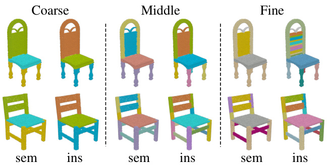
Figure 1: Illustration of 3D models with fine-grained and hierarchical part structures. Models are selected from PartNet [27]. From left to right: part semantics and part instances at the coarse, middle and fine level. Point colors are assigned to distinguish different part semantics and part instances.
图 1: 具有细粒度层级部件结构的3D模型示意图。模型选自PartNet [27]。从左至右分别为:粗粒度、中粒度和细粒度层级的部件语义及部件实例。通过点着色区分不同部件语义与部件实例。
Our semantic segmentation-assisted instance feature fusion scheme is simple and lightweight; it is not limited to 3D part instance segmentation and can be extended to 3D instance segmentation for indoor scenes. We integrated several state-of-the-art 3D instance segmentation frameworks with our feature fusion scheme and observed consistent improvements on the benchmark of ScanNet [8] and S3DIS [2], which demonstrate the efficacy and generality of our approach.
我们的语义分割辅助实例特征融合方案简单轻量,不仅限于3D部件实例分割,还可扩展至室内场景的3D实例分割任务。我们将多个前沿的3D实例分割框架与特征融合方案结合,在ScanNet [8] 和 S3DIS [2] 基准测试中均观察到性能提升,证明了该方法的有效性和普适性。
Contributions We make two contributions to tackle 3D instance segmentation: (1) We propose an instance feature fusion strategy that directly fuses instance features in a nonlocal way according to the guidance of semantic segmentation to improve instance center prediction. This strategy is lightweight and easily incorporated into many 3D instance segmentation frameworks for both 3D object and part instance segmentation. (2) Our multi- and cross-level instance feature fusion and the use of the semantic region center are effective for multi-level part instance segmentation and achieve the best performance on the PartNet bench- mark. Our code and trained models are publicly available at https://isunchy.github.io/projects/3d_ instance segmentation.html.
贡献
我们在3D实例分割方面做出了两项贡献:(1) 提出了一种实例特征融合策略,该策略根据语义分割的指导以非局部方式直接融合实例特征,从而改进实例中心预测。该策略轻量且易于集成到多种3D实例分割框架中,适用于3D物体和部件实例分割。(2) 我们的多层级与跨层级实例特征融合及语义区域中心的使用,对多层级部件实例分割有效,并在PartNet基准测试中取得了最佳性能。代码与训练模型已公开于https://isunchy.github.io/projects/3d_instance_segmentation.html。
2. Related Work
2. 相关工作
2D instance segmentation As surveyed by [14], four typical paradigms exist in the literature. The methods in the first paradigm generate mask proposals and then assign suitable shape semantics to the proposals [11, 30, 37]. The second one detects multiple objects using boxes and then extracts object masks within the boxes. Mask R-CNN [16] is one of the representative methods. The third is a bottom-up approach that predicts the semantic labels of each pixel and then groups pixels into 2D instances [3]. Its computation is relatively heavy due to per-pixel prediction. The fourth paradigm suggests using dense sliding windows techniques to generate mask proposals and mask scores for better instance segmentation [9, 5]. For detailed surveys, see articles [14, 44, 26].
2D实例分割
如[14]所述,文献中存在四种典型范式。第一种范式的方法先生成掩膜(mask)候选区域,再为候选区域分配合适的形状语义[11, 30, 37]。第二种方法先用边界框检测多个物体,再在框内提取物体掩膜,代表性方法是Mask R-CNN[16]。第三种是自底向上方法,先预测每个像素的语义标签,再将像素分组为2D实例[3],由于需要逐像素预测,计算量较大。第四种范式建议使用密集滑动窗口技术生成掩膜候选区域和掩膜分数,以获得更好的实例分割效果[9, 5]。详细综述可参阅文献[14, 44, 26]。
3D Instance segmentation The existing 3D approaches follow the paradigms of 2D instance segmentation (cf. surveys [13, 18]). Proposal-based methods [27, 20] predict a fixed number of instance segmentation masks and match them with the ground truth using the Hungarian algorithm or a trainable assignment module. The learned matching scores are used to group 3D points into instances. Detection-based methods [19, 40, 39, 10] generate highobjectness 3D proposals like boxes and then refine them to obtain instance masks.
3D实例分割
现有的3D方法遵循2D实例分割的范式(参见综述[13, 18])。基于提议的方法[27, 20]预测固定数量的实例分割掩码,并使用匈牙利算法或可训练的分配模块将其与真实标注匹配。学习到的匹配分数用于将3D点分组为实例。基于检测的方法[19, 40, 39, 10]生成高目标性的3D提议(如边界框),然后细化这些提议以获得实例掩码。
Clustering-based methods first produce per-point predictions and then use clustering methods to group points into instances. SGPN [36] predicts the similarity score of any two points and merges points into instance groups according to the scores. MASC [24] predicts the multiscale affinity between neighboring voxels, for instance, clustering. Hao et al. [15] regress the instance voxel occupancy for more accurate segmentation outputs. PointGroup [21] uses both the original and offset-shifted point sets to group points into candidate instances. DyCo3D [17] improves pointgroup by introducing a dynamic-convolution-based instance decoder. Observing that non-end-to-end clustered-based methods often exhibit over-segmentation and under-segmentation, Chen et al. [4] and Liang et al. [23] proposed mid-level shape representation to generate instance proposals hierarchically in an end-to-end training manner. Liu et al. [25] approximate the distributions of centers to select center candidates for instance prediction. As mentioned in Section 1, most cluster-based methods treat semantic segmentation and instance feature learning as multitasks; only the works of [38] and [45] fuse the network features of the instance prediction branch and the semantic segmentation branch to improve the performance of both branches. Unlike the pointwise fusion of [38] and [45], our method fuses instance features in a nonlocal manner guided by semantic outputs, which is more robust and effective.
基于聚类的方法首先生成逐点预测,随后通过聚类方法将点分组为实例。SGPN [36] 预测任意两点间的相似度分数,并依据分数将点合并为实例组。MASC [24] 预测相邻体素间的多尺度亲和力以实现聚类。Hao等 [15] 通过回归实例体素占用率来获得更精确的分割输出。PointGroup [21] 同时利用原始点集和偏移点集将点分组为候选实例。DyCo3D [17] 通过引入基于动态卷积的实例解码器改进了PointGroup。针对非端到端聚类方法常出现的过分割与欠分割问题,Chen等 [4] 和Liang等 [23] 提出中层形状表示法,以端到端训练方式分层生成实例提案。Liu等 [25] 通过中心分布近似来筛选实例预测的中心候选点。如第1节所述,多数基于聚类的方法将语义分割与实例特征学习视为多任务处理;仅[38]和[45]的工作通过融合实例预测分支与语义分割分支的网络特征来提升双分支性能。不同于[38]和[45]的逐点融合,我们的方法在语义输出引导下以非局部方式融合实例特征,具有更强的鲁棒性和有效性。
Part instance segmentation Different from object-level 3D instance segmentation, part-level 3D instance segmentation is less studied due to limited annotated data and the difficulty brought by geometry-similar but semantics-different shape parts. Mo et al. [27] present PartNet — a large-scale dataset of 3D objects with fine-grained, instance-level, and hierarchical part information. For the part instance segmentation task, they developed a detection-by-segmentation method and trained a specific network to extract part instances per structural level, where the semantic hierarchy was used for part instance segmentation. Other object-level instance segmentation methods, such as [17, 42], have also been extended to the task of part instance segmentation, but they do not use the semantic hierarchy. Yu et al. [41] further enriched PartNet with information about the binary hierarchy and designed a recursive neural network to perform recursive binary decomposition to extract 3D parts. Our multi- and cross-level instance feature fusion uses semantic hierarchy to improve instance center prediction. Furthermore, the use of semantic region centers assists instance grouping. The semantic region centers serve the role of symmetric centers of a group of semantics-same part instances and provide weak supervision to the training.
部件实例分割
与物体级3D实例分割不同,由于标注数据有限以及几何相似但语义不同的形状部件带来的困难,部件级3D实例分割的研究较少。Mo等人[27]提出了PartNet——一个包含细粒度、实例级和层次化部件信息的大规模3D物体数据集。针对部件实例分割任务,他们开发了一种基于分割的检测方法,并训练了特定网络来提取每个结构层级的部件实例,其中语义层次结构被用于部件实例分割。其他物体级实例分割方法(如[17, 42])也被扩展到部件实例分割任务,但未使用语义层次结构。Yu等人[41]进一步用二元层次结构信息丰富了PartNet,并设计了一个递归神经网络来执行递归二元分解以提取3D部件。我们的多层级和跨层级实例特征融合利用语义层次结构来改进实例中心预测。此外,语义区域中心的使用有助于实例分组。语义区域中心充当一组语义相同部件实例的对称中心角色,并为训练提供弱监督。
3. Methodology
3. 方法论
In this section, we first introduce our baseline neural network for single-level and multi-level 3D part instance segmentation in Section 3.1, then present the model enhanced by our semantic segmentation-assisted instance feature fusion module in Section 3.2 and the semantic region center prediction module in Section 3.3.
在本节中,我们首先在第3.1节介绍用于单层级和多层级3D零件实例分割的基线神经网络,然后在第3.2节展示通过语义分割辅助实例特征融合模块增强的模型,并在第3.3节介绍语义区域中心预测模块。
3.1. Baseline network
3.1. 基线网络
Our baseline network follows the encoder-decoder paradigm. The input to the encoder is a set of 3D points $s$ in which each point may be equipped with additional signals such as point normal and RGB color. Two parallel decoders are concatenated after the encoder to predict the point-wise semantic labels and the point offset to its corresponding instance center, named semantic decoder $D_{s e m}$ and instance decoder $D_{i n s}$ , respectively. The baseline network is depicted in Fig. 2, where the fusion module and semantic region center will be introduced in 3.2 and 3.3, respectively.
我们的基线网络遵循编码器-解码器范式。编码器的输入是一组3D点$s$,其中每个点可能附带法向量和RGB颜色等额外信号。编码器后连接两个并行解码器,分别用于预测逐点语义标签及其对应实例中心的点偏移量,称为语义解码器$D_{sem}$和实例解码器$D_{ins}$。基线网络结构如图2所示,其中融合模块和语义区域中心将分别在3.2和3.3节介绍。
The input points are shifted by the predicted offsets, and the shifted points with the same semantics are clustered into multiple 3D instances via the mean-shift algorithm [7]. In an ideal situation, all input points are shifted to their ground truth instance centers, but in practice, the accuracy of predicted offsets affects the performance of instance clustering.
输入点根据预测偏移量进行位移,通过均值漂移算法 [7] 将具有相同语义的位移点聚类为多个3D实例。理想情况下,所有输入点都应位移至其真实实例中心,但实际上预测偏移量的精度会影响实例聚类的性能。
Network structure We choose O-CNN-based U-Nets [34, 35] as our encoder-decoder structure. The network is built on octree-based CNNs , and its memory and computational efficiency are similar to those of other sparse convolutionbased neural networks [12, 6]. The input point cloud is converted to an octree first, whose non-empty finest octants store the average signal of the points contained by the octants. Both $D_{s e m}$ and $D_{i n s}$ output point-wise features via trilinear interpolation on sparse voxels: $F_{s e m},F_{i n s}\in\mathbb{R}^{N\times l}$ , where $N$ is the number of points and $l$ is the dimension of feature vectors.
网络结构 我们选择基于O-CNN的U-Net [34, 35]作为编码器-解码器结构。该网络建立在基于八叉树的CNN上,其内存和计算效率与其他基于稀疏卷积的神经网络 [12, 6] 相似。输入点云首先被转换为八叉树,其非空最精细八分区存储了该八分区所含点的平均信号。$D_{sem}$ 和 $D_{ins}$ 都通过对稀疏体素的三线性插值输出逐点特征:$F_{sem},F_{ins}\in\mathbb{R}^{N\times l}$,其中 $N$ 是点数,$l$ 是特征向量的维度。
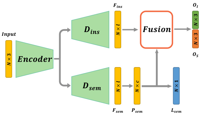
Figure 2: Illustration of our network architecture for single-level part instance segmentation. The network takes a 3D point cloud as input. $N$ is the point number. A shared encoder and two parallel decoders $D_{s e m},D_{i n s}$ are used to output the pointwise semantic feature $F_{s e m}$ and instance feature $F_{i n s}$ to predict the point semantic label $L_{s e m}$ and the offset vector $O_{I}$ to the instance center, and the offset vector $O_{S}$ to the semantic region center. The feature fusion module aggregates the instance features of points according to semantic segmentation probability vectors to improve the offset prediction.
图 2: 单层级部件实例分割的网络架构示意图。该网络以3D点云作为输入,$N$表示点数。通过共享编码器和两个并行解码器$D_{sem}$、$D_{ins}$分别输出逐点语义特征$F_{sem}$和实例特征$F_{ins}$,用于预测点的语义标签$L_{sem}$、到实例中心的偏移向量$O_{I}$以及到语义区域中心的偏移向量$O_{S}$。特征融合模块根据语义分割概率向量聚合点的实例特征,以提升偏移预测精度。
Semantic prediction and offset prediction A two-layer MLP is used to convert $F_{s e m}$ to the segmentation probability $P_{s e m}\in\mathbb{R}^{N\times c}$ , where $c$ is the number of semantic classes. The segmentation label $L_{s e m}$ is then determined from $P_{s e m}$ . The loss for training semantic segmentation is the standard cross-entropy loss.
语义预测与偏移预测
使用一个双层MLP将$F_{s e m}$转换为分割概率$P_{s e m}\in\mathbb{R}^{N\times c}$,其中$c$为语义类别数。分割标签$L_{s e m}$由$P_{s e m}$确定。语义分割训练的损失函数采用标准交叉熵损失。
$$
L_{s e m a n t i c}=\frac{1}{N}\sum_{i=1}^{N}C E(p_{i},p_{i}^{*}).
$$
$$
L_{s e m a n t i c}=\frac{1}{N}\sum_{i=1}^{N}C E(p_{i},p_{i}^{*}).
$$
Here, $p^{*}$ is the semantic label.
这里,$p^{*}$ 是语义标签。
Parallel to the semantic branch, another two-layer MLP maps $F_{i n s}$ to the offset tensor $O_{I}\in\mathbb{R}^{N\times3}$ , which is used to shift the input points to the center of the target instance. The loss for predicting the offsets is the $L_{2}$ loss between the prediction and the ground-truth offsets.
与语义分支并行,另一个双层MLP将 $F_{i n s}$ 映射到偏移张量 $O_{I}\in\mathbb{R}^{N\times3}$ ,用于将输入点移动到目标实例的中心。预测偏移的损失是预测值与真实偏移之间的 $L_{2}$ 损失。
$$
L_{o f f s e t}=\frac{1}{N}\sum_{i=1}^{N}||o_{i}-o_{i}^{*}||_{2}.
$$
$$
L_{o f f s e t}=\frac{1}{N}\sum_{i=1}^{N}||o_{i}-o_{i}^{*}||_{2}.
$$
Here, $o^{*}$ is the ground-truth offset.
这里,$o^{*}$ 是真实偏移量。
Instance clustering During the test phase, the network outputs pointwise semantics and offset vectors. We use the mean-shift algorithm to group the shifted points with the same semantics into disjointed instances.
实例聚类
在测试阶段,网络会逐点输出语义和偏移向量。我们使用均值漂移(mean-shift)算法将具有相同语义的偏移点分组为不连贯的实例。
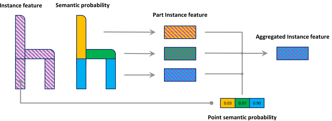
Figure 3: Semantic segmentation-assisted instance feature fusion pipeline. Given the per-point instance feature and semantic probability, we get the part instance features according to the instance feature of points associated with each semantic part. Then we obtain the aggregated instance feature for each point by combining part instance features using its semantic probability.
图 3: 语义分割辅助的实例特征融合流程。给定逐点实例特征和语义概率,我们根据与每个语义部分相关联的点的实例特征获取部件实例特征。随后通过结合各部件实例特征并利用其语义概率,得到每个点的聚合实例特征。
Multi-level part instances For shapes with hierarchical and multi-level part instances, there are two naive way to extend the baseline network: (1) train the baseline network for each level individually; (2) revise the baseline network to output multi-level semantics and multi-level offset vectors simultaneously by adding multi-prediction branches after $F_{i n s}$ and $F_{s e m}$ . We denote $K$ as the level number, add a superscript $k$ to all the symbols defined above to distinguish features at the $k$ -th level, like $F_{s e m}^{(k)},F_{i n s}^{(k)},P_{s e m}^{(k)},c^{(k)},\check{O}_{I}^{(k)}$ .
多层次部件实例
对于具有层次结构和多层次部件实例的形状,有两种简单的方法来扩展基线网络:(1) 为每个级别单独训练基线网络;(2) 通过在 $F_{ins}$ 和 $F_{sem}$ 后添加多预测分支,修改基线网络以同时输出多层次语义和多层次偏移向量。我们将 $K$ 表示为级别数,并为上述所有符号添加一个上标 $k$ 以区分第 $k$ 层的特征,例如 $F_{sem}^{(k)},F_{ins}^{(k)},P_{sem}^{(k)},c^{(k)},\check{O}_{I}^{(k)}$。
3.2. Semantic segmentation-assisted instance feature fusion
3.2. 语义分割辅助的实例特征融合
3.2.1 Single-level instance feature fusion
3.2.1 单层级实例特征融合
As the points within the same instance possess the same instance center, it is essential to aggregate the instance features over these points to regress the offset to the instance center robustly. However, these points are not known during the network inference stage and they are also the objective of the task. The semantic decoder branch can predict the semantic region composed by a set of part instances; we can aggregate the instance features over the semantic parts to provide nonlocal guidance to the input points. We propose a semantic segmentation-assisted instance feature fusion module that contains two steps. In the first step, for each semantic part, we compute the instance feature based on the points associated with this part. Each point is associated with an aggregated instance feature from semantic parts in the second step according to its semantic probability vector. The instance feature fusion pipeline is illustrated in Fig. 3. Our feature aggregation procedure is as follows.
由于同一实例内的点共享相同的实例中心,因此需要聚合这些点上的实例特征以稳健地回归到实例中心的偏移量。然而,在网络推理阶段这些点尚未可知,它们本身也是任务的目标。语义解码器分支可预测由一组部件实例构成的语义区域,我们能够通过聚合语义部件上的实例特征为输入点提供非局部引导。我们提出了一个包含两步操作的语义分割辅助实例特征融合模块:第一步,针对每个语义部件,基于与该部件关联的点计算实例特征;第二步,根据各点的语义概率向量,为其关联来自语义部件的聚合实例特征。图3展示了该实例特征融合流程,具体聚合步骤如下。
Part instance feature We first aggregate the instance features with respect to the semantic label $m\in{1,\ldots,c}$ over
部件实例特征
我们首先针对语义标签 $m\in{1,\ldots,c}$ 聚合实例特征
the input:
输入:
$$
Z_{m}:=\frac{\sum_{\mathbf{p}\in\mathcal{S}}P_{s e m}(\mathbf{p})|{m}\cdot F_{i n s}(\mathbf{p})}{\sum_{\mathbf{p}\in\mathcal{S}}P_{s e m}(\mathbf{p})|_{m}}.
$$
$$
Z_{m}:=\frac{\sum_{\mathbf{p}\in\mathcal{S}}P_{s e m}(\mathbf{p})|{m}\cdot F_{i n s}(\mathbf{p})}{\sum_{\mathbf{p}\in\mathcal{S}}P_{s e m}(\mathbf{p})|_{m}}.
$$
$Z_{m}$ is the aggregated instance feature for the semantic part with semantic label of $m$ , $P_{s e m}(\mathbf{p})|_{m}$ is the probability value of point $\mathbf{p}$ with respect to the semantic label $m$ .
$Z_{m}$ 是具有语义标签 $m$ 的语义部分的聚合实例特征, $P_{sem}(\mathbf{p})|_{m}$ 是点 $\mathbf{p}$ 相对于语义标签 $m$ 的概率值。
Aggregated instance feature For each point $\mathbf{p}$ , we aggregate the instance feature $Z_{m}\mathbf{s}$ using the semantic probability of $\mathbf{p}$ as follows:
聚合实例特征 对于每个点 $\mathbf{p}$,我们使用 $\mathbf{p}$ 的语义概率聚合实例特征 $Z_{m}\mathbf{s}$,具体如下:
$$
\hat{F}(\mathbf{p})=\sum_{m=1}^{c}P_{s e m}(\mathbf{p})|{m}\cdot Z_{m}.
$$
$$
\hat{F}(\mathbf{p})=\sum_{m=1}^{c}P_{s e m}(\mathbf{p})|{m}\cdot Z_{m}.
$$
The above equations for all points can be written in matrix form: $\mathbf{Z}=(\mathbf{P_{sem}^{\star}}/\left(\mathbf{I_{1}}\mathbf{P_{sem}}\right))^{T}\mathbf{F_{ins}},\hat{\mathbf{F}}=\mathbf{P_{sem}}\mathbf{Z}$ , where $\mathbf{Z}\in\mathbb{R}^{c\times l}$ , $\mathbf{P_{sem}}\in\mathbb{R}^{N\times c}$ , $\mathbf{F_{ins}}\in\mathbb{R}^{N\times l}$ , $\hat{\mathbf{F}}\in\mathbb{R}^{N\times l}$ , ${\bf{I}_{1}}$ is an $N\times N$ matrix with all ones, and $\mathbf{\mu}^{\leftarrow}/\mathbf{\eta}^{\rightarrow}$ represents elementwise division.
所有点的上述方程可以写成矩阵形式:$\mathbf{Z}=(\mathbf{P_{sem}^{\star}}/\left(\mathbf{I_{1}}\mathbf{P_{sem}}\right))^{T}\mathbf{F_{ins}},\hat{\mathbf{F}}=\mathbf{P_{sem}}\mathbf{Z}$,其中$\mathbf{Z}\in\mathbb{R}^{c\times l}$,$\mathbf{P_{sem}}\in\mathbb{R}^{N\times c}$,$\mathbf{F_{ins}}\in\mathbb{R}^{N\times l}$,$\hat{\mathbf{F}}\in\mathbb{R}^{N\times l}$,${\bf{I}_{1}}$是一个全1的$N\times N$矩阵,$\mathbf{\mu}^{\leftarrow}/\mathbf{\eta}^{\rightarrow}$表示逐元素除法。
We concatenate the aggregated instance feature ${\hat{F}}(\mathbf{p})$ , the local instance feature $F_{i n s}(\mathbf{p})$ and the position of $\mathbf{p}$ to form a fused instance feature $F_{f u s i o n}(\mathbf{p}):=[\hat{F}(\mathbf{p}),{F}_{i n s}(\mathbf{p}),\mathbf{p}]$ , and use it to predict the instance center offset. Fig. 4-(a) illustrates our feature fusion module for a single level. The overall network structure is shown in Fig. 2.
我们将聚合实例特征 ${\hat{F}}(\mathbf{p})$、局部实例特征 $F_{i n s}(\mathbf{p})$ 和点 $\mathbf{p}$ 的位置拼接形成融合实例特征 $F_{f u s i o n}(\mathbf{p}):=[\hat{F}(\mathbf{p}),{F}_{i n s}(\mathbf{p}),\mathbf{p}]$,并利用该特征预测实例中心偏移量。图4-(a)展示了单层级的特征融合模块结构,整体网络架构如图2所示。
3.2.2 Multi-level instance feature fusion
3.2.2 多层级实例特征融合
For shapes with multi-level part instances, our single-level instance feature fusion can be applied to each level individually. The naively extended baseline networks (Section 3.1) can benefit from this kind of instance feature fusion for multi-level part instance segmentation.
对于具有多层级部件实例的形状,我们的单层级实例特征融合可以分别应用于每个层级。这种实例特征融合能够帮助朴素扩展的基线网络(第3.1节)提升多层级部件实例分割的效果。
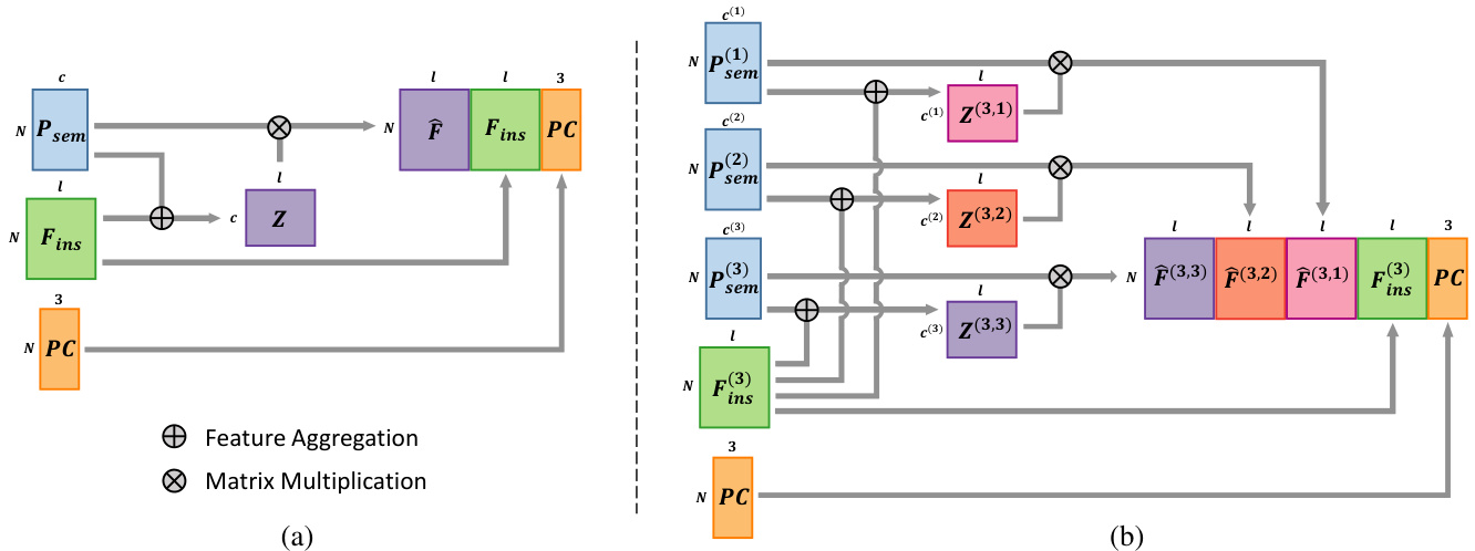
Figure 4: Semantic segmentation-assisted instance feature fusion for single-level and cross-level. (a) Single-level instance feature fusion. Instance features $\mathbf{F_{ins}}$ are aggregated to $\hat{\mathbf{F}}$ , with the help of semantic probability vectors $\mathbf{P_{sem}}$ . $\hat{\mathbf{F}}$ , $\mathbf{F_{ins}}$ and the point position PC are assembled to form the fused instance features $\mathbf{F_{fusion}}$ . (b) Cross-level instance feature fusion for a 3-level part instance segmentation. The fused features at the 3rd level are depicted. For clarity, we omit fused features at other levels.
图 4: 单层级与跨层级的语义分割辅助实例特征融合。(a) 单层级实例特征融合。实例特征 $\mathbf{F_{ins}}$ 在语义概率向量 $\mathbf{P_{sem}}$ 的辅助下聚合为 $\hat{\mathbf{F}}$ 。$\hat{\mathbf{F}}$ 、$\mathbf{F_{ins}}$ 与点云位置 PC 组合形成融合实例特征 $\mathbf{F_{fusion}}$ 。(b) 3层级部件实例分割的跨层级特征融合。图中展示了第3层级的融合特征,为简化示意图省略了其他层级的融合特征。
3.2.3 Cross-level instance feature fusion
3.2.3 跨层级实例特征融合
When multi-level part instances and semantic segmentation exhibit a hierarchical relationship, i.e. , the fine-level part instances are contained within the coarser-level part instances and can inherit the semantics from their parent level, we leverage the semantic segmentation in multi-levels to fuse instance features at each level, we call our strategy crosslevel instance feature fusion. The exact fusion procedure is as follows.
当多级部件实例与语义分割呈现层级关系时(即细粒度部件实例包含在粗粒度部件实例中,并可从父级继承语义),我们利用多级语义分割来融合每一级的实例特征,这种策略称为跨级实例特征融合。具体融合流程如下。
Instance feature aggregation On level $k$ , we aggregate the instance features using semantic probability vectors at the $r$ -th level:
实例特征聚合
在层级 $k$ 上,我们使用第 $r$ 层级的语义概率向量聚合实例特征:
$$
Z_{m}^{(k,r)}:=\frac{\sum_{{\bf{q}}\in{\cal{S}}}P_{s e m}^{(r)}({\bf{q}})|{m}\cdot F_{i n s}^{(k)}({\bf{q}})}{\sum_{{\bf{q}}\in{\cal{S}}}P_{s e m}^{(r)}({\bf{q}})|_{m}},m\in{1,\ldots,c^{(r)}}.
$$
$$
Z_{m}^{(k,r)}:=\frac{\sum_{{\bf{q}}\in{\cal{S}}}P_{s e m}^{(r)}({\bf{q}})|{m}\cdot F_{i n s}^{(k)}({\bf{q}})}{\sum_{{\bf{q}}\in{\cal{S}}}P_{s e m}^{(r)}({\bf{q}})|_{m}},m\in{1,\ldots,c^{(r)}}.
$$
$Z_{m}^{(k,r)}\mathbf{s}$ are then averaged at point $\mathbf{p}$ at the $k$ -th level:
在第 $k$ 层,将 $Z_{m}^{(k,r)}\mathbf{s}$ 在点 $\mathbf{p}$ 处进行平均:
$$
\hat{F}^{(k,r)}(\mathbf{p})=\sum_{m=1}^{c^{(r)}}P_{s e m}^{(r)}(\mathbf{p})|{m}\cdot Z_{m}^{(k,r)}.
$$
$$
\hat{F}^{(k,r)}(\mathbf{p})=\sum_{m=1}^{c^{(r)}}P_{s e m}^{(r)}(\mathbf{p})|{m}\cdot Z_{m}^{(k,r)}.
$$
The fused instance feature of $\mathbf{p}$ at the $k$ -th level is defined as follows:
$\mathbf{p}$ 在第 $k$ 层的融合实例特征定义如下:
$$
F_{f u s i o n}^{(k)}(\mathbf{p}):=[\hat{F}^{(k,1)}(\mathbf{p}),\cdot\cdot\cdot,\hat{F}^{(k,K)}(\mathbf{p}),F_{i n s}^{(k)}(\mathbf{p}),\mathbf{p}].
$$
$$
F_{f u s i o n}^{(k)}(\mathbf{p}):=[\hat{F}^{(k,1)}(\mathbf{p}),\cdot\cdot\cdot,\hat{F}^{(k,K)}(\mathbf{p}),F_{i n s}^{(k)}(\mathbf{p}),\mathbf{p}].
$$
It is mapped to offset vectors at the $k$ -th level by an MLP layer. We illustrate the cross-level instance feature fusion in Fig. 4-(b).
它通过一个MLP层被映射到第$k$层的偏移向量。我们在图4-(b)中展示了跨层级实例特征融合。
3.3. Semantic region center
3.3. 语义区域中心
During the test phase, we use the mean-shift algorithm to split the offset-shifted points with the same semantics into different instances. For 3D instances which are close to each other, like two blades of a scissor shown in Fig. 5-(a), it is difficult to separate the points belonging to them using mean-shift or other 3D point clustering algorithms, as the instance centers are very close to each other (see Fig. 5-(b)). We introduce the concept of semantic region center, which is the center of semantically -same instance centers. The semantic region center is usually the center of symmetrically arranged parts for human-made shapes Fig. 5-(c) illustrates the semantic region centers. To make instance clustering easy, the instance centers can be further shifted away from the semantic region center, as shown Fig. 5-(d). In the offset prediction branch of our network, we also add the offset prediction $O_{S}$ to the center of the semantic region for each point.
在测试阶段,我们使用均值漂移算法将具有相同语义的偏移点分割到不同实例中。对于彼此靠近的3D实例(如图5-(a)所示的剪刀两片刀刃),由于实例中心非常接近(见图5-(b)),使用均值漂移或其他3D点聚类算法难以分离属于它们的点。我们引入了语义区域中心的概念,即语义相同实例中心的中心点。对于人造形状,语义区域中心通常是对称排列部件的中心,图5-(c)展示了语义区域中心。为简化实例聚类,实例中心可进一步远离语义区域中心进行偏移,如图5-(d)所示。在网络偏移预测分支中,我们还为每个点增加了指向语义区域中心的偏移预测$O_{S}$。
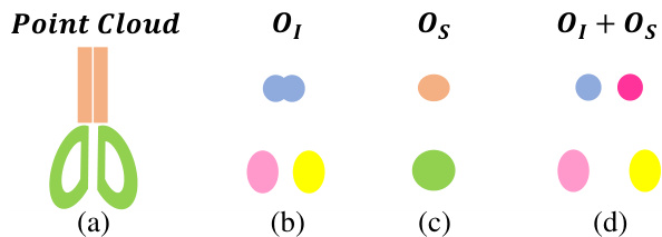
Figure 5: Illustration of the use of semantic region centers. (a) Input point cloud of a scissor shape. Ground-truth part instances are colored according to their semantics. (b) Predicted instance centers. (c) Predicted semantic region centers. (d) By pushing the predicted instance centers away from the predicted semantic region centers, the shifted instance centers of the scissor blades become more distinguishable than in(b).
图 5: 语义区域中心的使用示意图。(a) 剪刀形状的输入点云,真实部件实例按其语义着色。(b) 预测的实例中心。(c) 预测的语义区域中心。(d) 通过将预测的实例中心推离预测的语义区域中心,剪刀刀片的偏移实例中心比(b)中更具区分性。
In the instance clustering step, we shift the input points as follows:
在实例聚类步骤中,我们对输入点进行如下位移:
$$
\hat{\mathbf{p}}:=\mathbf{p}+O_{I}(\mathbf{p})+\lambda\cdot\frac{O_{I}(\mathbf{p})-O_{S}(\mathbf{p})}{||O_{I}(\mathbf{p})-O_{S}(\mathbf{p})||}.
$$
$$
\hat{\mathbf{p}}:=\mathbf{p}+O_{I}(\mathbf{p})+\lambda\cdot\frac{O_{I}(\mathbf{p})-O_{S}(\mathbf{p})}{||O_{I}(\mathbf{p})-O_{S}(\mathbf{p})||}.
$$
Here $\mathbf{p}\in{\mathcal{S}},\lambda>0$ .
这里 $\mathbf{p}\in{\mathcal{S}},\lambda>0$ 。
Table 1: Part instance segmentation results of the test set on PartNet [27]. We report part-category $A P_{50}$ on three instance levels. The results of other methods are reported by PE [42]. Bold numbers are better. Some shape categories, masked by dashed lines, have no middle- and fine-level instances for benchmark.
表 1: PartNet [27] 测试集上的部件实例分割结果。我们在三个实例级别上报告了部件类别的 $A P_{50}$。其他方法的结果由 PE [42] 报告。加粗数字表示更优。部分形状类别(用虚线标记)在基准测试中没有中等级别和精细级别的实例。
4. Experiments and Analysis
4. 实验与分析
We design a series of experiments and ablation studies to demonstrate the efficacy of our approach and its superiority to other fusion schemes, including multi-level part instance segmentation on PartNet [27] (Section 4.1), and instance segmentation on indoor scene datasets (Section 4.2): ScanNet [8] and S3DIS [2].
我们设计了一系列实验和消融研究来证明方法的有效性及其相对于其他融合方案的优势,包括在PartNet [27]上的多层次部件实例分割(第4.1节)以及室内场景数据集(ScanNet [8]和S3DIS [2])上的实例分割(第4.2节)。
4.1. Part instance segmentation on PartNet
4.1 PartNet 上的部件实例分割
4.1.1 Experiments and comparison
4.1.1 实验与对比
Dataset PartNet is a large-scale dataset with fine-grained and hierarchical part annotations. It contains more than $570\mathrm{k}$ part instances over 26,671 3D models covering 24 object categories. It provides coarse-, middle-, and fine-grained part instance annotations.
数据集 PartNet 是一个具有细粒度和层次化部件标注的大规模数据集。它包含超过 $570\mathrm{k}$ 个部件实例,覆盖 26,671 个 3D 模型,涵盖 24 个物体类别。该数据集提供了粗粒度、中粒度和细粒度的部件实例标注。
Network configuration The encoder and decoders of our O-CNN-based U-Net had five levels of domain resolution, and the maximum depth of the octree was six. The dimension of the feature was set to 64. Details of the U-Net structure are provided in Appendix A. We implemented our network in the TensorFlow framework [1]. The network was trained with 100000 iterations with a batch size of 8. We used the SGD optimizer with a learning rate of 0.1 and decay two times with the factor of 0.1 at the 50000-th and 75000-th iterations. Our code and trained models are available.
网络配置
我们基于O-CNN的U-Net编码器和解码器具有五级域分辨率,八叉树的最大深度为6。特征维度设置为64。U-Net结构的详细信息见附录A。我们在TensorFlow框架[1]中实现了该网络。网络训练了100000次迭代,批量大小为8。我们使用学习率为0.1的SGD优化器,并在第50000次和第75000次迭代时以0.1的因子进行两次衰减。我们的代码和训练模型已公开。
Data processing The input point cloud contained 10 000 points and was scaled into a unit sphere. During training, we also augmented each shape by a uniform scaling with the scale ratio of [0.75, 1, 25], a random rotation whose pitch, yaw, and roll rotation angles were less than $10^{\circ}$ , and random translations along each coordinate axis within the interval $[-0.125,0.125]$ . The train/test split is provided in PartNet. Note that not all categories have three-level part annotations. During training, we duplicated the labels at the coarser level to the finer level, if the latter was missing, to mimic the three-level shape structure. During the test phase, we only evaluated the output from the levels which exist in the data. The ground-truth instance centers and semantic region centers were pre-computed according to the semantic labels and part instances of PartNet.
数据处理
输入点云包含10,000个点,并被缩放至单位球体内。训练过程中,我们通过以下方式对每个形状进行数据增强:均匀缩放比例范围为[0.75, 1.25],随机旋转(俯仰角、偏航角和滚转角均小于$10^{\circ}$),以及沿各坐标轴在区间$[-0.125,0.125]$内的随机平移。训练/测试划分由PartNet提供。需注意并非所有类别都具备三级部件标注。训练时,若较细级别的标注缺失,我们会将较粗级别的标签复制至该级别以模拟三级形状结构。测试阶段仅评估数据中实际存在的级别输出。根据PartNet的语义标签和部件实例,我们预先计算了真实实例中心和语义区域中心。
Experiment setup We set $\lambda~=~0.05$ for Eq. (7). We used the mean-shift implementation implemented in scikitlearn [28]. The default bandwidth of mean-shift was set to 0.1. All our experiments were conducted on an Azure Linux server with Intel Xeon Platinum 8168 CPU (2.7 GHz) and Tesla V100 GPU (16 GB memory). Our baseline network with cross-level fusion was the default configuration. In practice, we found that stopping the gradient from the fusion module to the semantic decoder helps maintain the semantic segmentation accuracy and slightly improves the instance segmentation. So, we enabled gradient stopping by default. An ablation study on gradient stopping is provided in Section 4.1.2.
实验设置
我们在公式(7)中设定$\lambda~=~0.05$。采用scikitlearn[28]实现的均值漂移算法,其默认带宽设为0.1。所有实验均在配备Intel Xeon Platinum 8168处理器(2.7 GHz)和Tesla V100显卡(16GB显存)的Azure Linux服务器上完成。基线网络采用默认的跨层级融合配置。实验发现,阻断融合模块至语义解码器的梯度流有助于保持语义分割精度,同时小幅提升实例分割效果,因此默认启用了梯度阻断机制。梯度阻断的消融实验详见第4.1.2节。
Evaluation metrics We used per-category mAP score with the IoU threshold of 0.25, 0.5 and 0.75 to evaluate the quality of part instance segmentation. They are denoted by $A P_{25}$ , $A P_{50}$ and $A P_{75}$ . ${\bf s}{-}A P_{50}$ is the metric proposed by [27], which averages the precision over the shapes.
评估指标
我们采用每类别的mAP分数,IoU阈值为0.25、0.5和0.75,以评估部件实例分割的质量。这些分数分别表示为$A P_{25}$、$A P_{50}$和$A P_{75}$。${\bf s}{-}A P_{50}$是[27]提出的指标,它对形状上的精度进行平均。
Performance report and comparison We report $A P_{50}$ of our approach in all 24 shape categories in Table 1. We also report the performance of three comparison approaches: SGPN [36], PartNet [27], and PE [42]. The results are averaged over three levels of granularity. Our method outperformed the best competitor PE [42] by $6.6%$ , and also achieved the best performance in most categories. Our approach was also the best on other evaluation metrics, as shown in Table 2. Appendix C reports the per-category results of $A P_{25}$ , $A P_{75}$ and ${\bf s}{-}A P_{50}$ . As DyCo3D [17] only performed instance segmentation experiments in four categories of the PartNet dataset, we compare it with our approach on these categories separately in Table 3. Our method outperformed DyCo3D by a large margin.
性能报告与对比
我们在表1中报告了本方法在所有24种形状类别中的$AP_{50}$值,同时列出了三种对比方法(SGPN [36]、PartNet [27] 和 PE [42])的性能表现。所有结果均按三个粒度层级取平均值。我们的方法以$6.6%$的优势超越最佳竞争对手PE [42],并在大多数类别中取得最优表现。如表2所示,本方法在其他评估指标上同样保持领先。附录C详细列出了$AP_{25}$、$AP_{75}$和${\bf s}{-}AP_{50}$的逐类别结果。由于DyCo3D [17]仅在PartNet数据集的四个类别中进行了实例分割实验,我们在表3中单独比较了这些类别的结果,本方法以显著优势超越DyCo3D。
Table 2: Part instance segmentation on the test set of PartNet. $A P_{25}$ $,A P_{50},A P_{75}$ , $\mathrm{s}{-}A P_{50}$ are averaged over three levels. The results of other methods are reported by PartNet [27] and PE [42].
表 2: PartNet 测试集上的部件实例分割结果。$A P_{25}$、$A P_{50}$、$A P_{75}$ 和 $\mathrm{s}{-}A P_{50}$ 为三个层级的平均值。其他方法的结果来自 PartNet [27] 和 PE [42]。
| AP25 | AP50 | AP75 | S-AP50 | mloU | |
|---|---|---|---|---|---|
| SGPN[36] | 46.8 | - | 64.2 | ||
| PartNet [27] | 62.8 | 54.4 | 38.9 | 72.2 | |
| PE [42] | 66.5 | 57.5 | 41.7 | - | - |
| Ours | 72.1 | 64.1 | 49.7 | 76.1 | 66.1 |
Table 3: Part instance segmentation on the four categories of PartNet. $A P_{50}$ is reported.
表 3: PartNet四类别的部件实例分割结果。报告指标为 $A P_{50}$。
| Level | Chair | Lamp | Stora. | Table | |
|---|---|---|---|---|---|
| D 3 | Coarse | 81.0 | 37.3 | 44.5 | 55.0 |
| Middle | 41.3 | 28.8 | 38.9 | 32.5 | |
| Fine | 33.4 51.9 | 20.5 | 30.4 | 24.9 | |
| Avg Coarse Middle | 84.1 45.7 | 28.9 38.2 | 37.9 56.4 | 37.5 65.3 | |
| sino | Fine | 38.2 | 30.9 21.7 | 53.3 44.0 | 36.2 28.9 |
| Avg | 56.0 | 30.3 | 51.2 | 43.5 |
4.1.2 Ablation study
4.1.2 消融实验
We validated our network design on PartNet instance segmentation, especially for the fusion module and the semantic region centers. The variants of our network are listed below.
我们在PartNet实例分割任务上验证了网络设计,特别是融合模块和语义区域中心部分。网络变体如下所示。
For each variant, we use symbol $\dagger$ to indicate that the predicted semantic region centers are not used for instance clustering. The optimal variant is cross-level fusion. The performance of each variant is reported in Table 4.
对于每个变体,我们用符号 $\dagger$ 表示预测的语义区域中心未用于实例聚类。最佳变体是跨层级融合。各变体的性能如表 4 所示。
Table 4: Ablation studies of our approach on PartNet test data. Methods marked with $\dagger$ use the predicted instance centers only. Our default and optimal network setting is cross-level fusion.
表 4: 我们的方法在PartNet测试数据上的消融研究。标记为$\dagger$的方法仅使用预测的实例中心。我们的默认和最优网络设置是跨层级融合(cross-level fusion)。
| 方法 | AP25 | AP50 | AP75 | S-AP50 | mloU |
|---|---|---|---|---|---|
| 单层级基线(single-level baseline) | 67.3 | 57.9 | 45.3 | 74.4 | 64.9 |
| 单层级基线(single-level baseline) | 67.4 | 58.2 | 45.5 | 75.0 | 64.9 |
| 单层级融合$\dagger$(single-level fusion$\dagger$) | 70.4 | 61.2 | 48.8 | 74.8 | 65.4 |
| 单层级融合(single-level fusion) | 71.1 | 62.1 | 49.0 | 75.8 | 65.4 |
| 多层级基线(multi-level baseline) | 67.1 | 57.9 | 45.0 | 74.1 | 65.0 |
| 多层级基线(multi-level baseline) | 67.3 | 58.1 | 45.1 | 74.7 | 65.0 |
| 多层级融合$\dagger$(multi-level fusion$\dagger$) | 70.9 | 61.8 | 48.8 | 74.8 | 65.5 |
| 多层级融合(multi-level fusion) | 71.5 | 62.5 | 49.2 | 75.6 | 65.5 |
| 跨层级融合(cross-level fusion) | 71.3 | 63.1 | 48.6 | 75.2 | 66.1 |
| 跨层级融合(cross-level fusion) | 72.1 | 64.1 | 49.7 | 76.1 | 66.1 |
| 跨层级融合(梯度)(cross-level fusion(gradient)) | 71.1 | 62.2 | 48.4 | 75.0 | 65.2 |
| 跨层级融合(梯度)(cross-level fusion(gradient)) | 71.8 | 63.3 | 49.3 | 75.9 | 65.2 |
| 跨层级融合(独热)$\dagger$(cross-level fusion(one-hot)$\dagger$) | 70.7 | 62.4 | 48.1 | 75.0 | 65.8 |
| 跨层级融合(独热)(cross-level fusion(one-hot)) | 71.6 | 63.5 | 49.0 | 75.8 | 65.8 |
| 跨层级融合(主干)$\dagger$(cross-level fusion(backbone)$\dagger$) | 69.6 | 61.6 | 46.0 | 74.7 | 65.3 |
| 跨层级融合(主干)(cross-level fusion(backbone)) | 70.2 | 62.4 | 47.1 | 75.3 | 65.3 |
| 跨层级融合(双向)(cross-level fusion(two-dir)) | 71.0 | 62.6 | 48.3 | 75.2 | 65.7 |
| 跨层级融合(双向)(cross-level fusion(two-dir)) | 71.8 | 63.6 | 48.7 | 76.0 | 65.7 |
| ASIS融合$\dagger$(ASIS fusion$\dagger$) | 68.2 | 59.0 | 45.0 | 74.7 | 65.1 |
| ASIS融合(ASIS fusion) | 68.6 | 59.1 | 45.9 | 75.0 | 65.1 |
| JSNet融合(JSNet fusion) | 68.5 | 59.2 | 46.3 | 75.4 | 65.4 |
| JSNet融合(JSNet fusion) | 68.8 | 59.3 | 46.6 | 75.6 | 65.4 |
Single-level baseline versus multi-level baseline The performances of single-level baseline and multi-level baseline in the same setting (w. or w/o fusion and semantic region center) are not much different. However, the training effort of multi-level baseline is much lower. There are a total of 50 levels for all 24 categories of PartNet. The single-level baseline must train 50 networks, while the multi-level baseline only needs to train 24 networks.
单层基线与多层基线的比较
在相同设置下(无论是否融合及使用语义区域中心),单层基线和多层基线的性能差异不大。然而,多层基线的训练成本显著更低。PartNet的24个类别共有50个层级,单层基线需训练50个网络,而多层基线仅需训练24个网络。
Fusion module It is clear that the performance of all baselines with the fusion modules improved. Single-level fusion and multi-level fusion increase $A P_{50}$ by $+3.9$ and $+4.4$ points compared to their baselines. Cross-level fusion surpasses them at $A P_{50}$ by $+2.0$ and $+1.6$ points. Here, the network of cross-level fusion has a slightly large network size. On Chair category, the network parameters of cross-level fusion, multi-level fusion, multi-level baselines are 8.13 M, 7.98 M, and $7.89\mathrm{M}$ , respectively.
融合模块
显然,所有带有融合模块的基线性能均有所提升。单级融合和多级融合相比其基线在 $AP_{50}$ 上分别提升了 $+3.9$ 和 $+4.4$ 个百分点。跨级融合在 $AP_{50}$ 上进一步超越它们,分别高出 $+2.0$ 和 $+1.6$ 个百分点。此处,跨级融合的网络规模略大。在 Chair 类别中,跨级融合、多级融合和多级基线的网络参数量分别为 8.13 M、7.98 M 和 $7.89\mathrm{M}$。
Use of semantic region centers The instance segmentation performance is consistently improved by using semantic region centers. The improvement is also more noticeable when the fusion module is enabled to improve both the instance center prediction and the semantic region center prediction. For example, there is only $+(0.2\sim0.3)$ improvement when using semantic region centers on single-level baseline and multi-level baseline, while the improvement over cross-level fusion $\dagger$ is $+1.0$ .
使用语义区域中心
通过使用语义区域中心,实例分割性能得到持续提升。当启用融合模块以同时改进实例中心预测和语义区域中心预测时,提升效果更为显著。例如,在单层级基线和多层级基线上使用语义区域中心时仅带来 $+(0.2\sim0.3)$ 的提升,而对跨层级融合 $\dagger$ 的提升达到 $+1.0$。
In Fig. 6, we present the instance segmentation results of multi-level baseline, cross-level fusion† and cross-level fusion. The predicted instance centers are more compact and distinguishable when using the fusion module. The use of semantic region centers helps further separate close instances, e.g. , the scissor blades in the 1st column, the bag handles in the 2nd column and the chair back frames in the 7th column.
在图 6 中,我们展示了多级基线、跨级融合†和跨级融合的实例分割结果。使用融合模块时,预测的实例中心更加紧凑且易于区分。语义区域中心的使用有助于进一步分离相邻实例,例如第 1 列中的剪刀刃、第 2 列中的包把手以及第 7 列中的椅背框架。
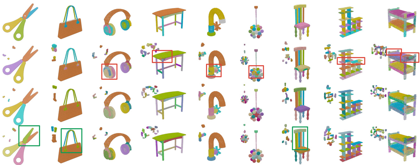
Figure 6: Visual comparison of part instance segmentation on the test set of PartNet. Part instances at the fine level are colored with random colors. 1st row: part instance ground-truth. 2nd row: results of our multi-level baseline†. 3rd row: results of our cross-level fusion† without using semantic region centers. 4th row: results of our cross-level fusion using semantic region centers. The corresponding shifted points are rendered at the top left of each instance segmentation image. Green and red boxes represent good and bad instances, respectively.
图 6: PartNet测试集上部件实例分割的视觉对比。精细层级的部件实例采用随机颜色标注。第1行: 部件实例真实标注。第2行: 我们的多层级基线†结果。第3行: 未使用语义区域中心的跨层级融合†结果。第4行: 采用语义区域中心的跨层级融合结果。对应的偏移点渲染在每张实例分割图像的左上角。绿色和红色方框分别表示良好与欠佳的实例。
Stopping gradient One of the inputs of the fusion module is the semantic segmentation probability. The gradients of the fusion module can back propagate the errors to the semantic branch. In our experiments, we found that gradient back propagation impairs semantic segmentation and leads to slightly worse instance segmentation results (see cross-level fusion(gradient) in Table 4).
停止梯度 (Stopping gradient)
融合模块的输入之一是语义分割概率。融合模块的梯度会将误差反向传播至语义分支。实验中我们发现,梯度反向传播会损害语义分割性能,并导致实例分割结果略微下降 (见表 4 中的跨层级融合(梯度) )。
Instance feature aggregation In our instance feature fusion module, we used the semantic probability of the point to aggregate the instance features from different semantic parts. An alternative way is to aggregate the instance features of the part which the point belongs to, i.e. , using the one-hot version of semantic probability for each point. We found that our default fusion is better than this alternative (cross-level fusion(one-hot) in Table 4) because the instance features from different semantic parts can bring more contextual information, especially for points with fuzzy semantic probability.
实例特征聚合
在我们的实例特征融合模块中,我们利用点的语义概率来聚合来自不同语义部分的实例特征。另一种方法是聚合点所属部分的实例特征,即对每个点使用独热编码(one-hot)版本的语义概率。我们发现默认的融合方式优于这种替代方案(表4中的跨层级融合(one-hot)),因为来自不同语义部分的实例特征能提供更多上下文信息,尤其对于具有模糊语义概率的点。
Network backbone The O-CNN [34, 35] backbone used in our network is different from the PointNet+ $+$ [29] backbone used in [27, 42]. Therefore, we also replaced the O-CNN backbone with PointNet $^{;++}$ for a fair comparison. As shown in cross-level fusion(backbone) in Table 4, the performance of the PointNet+ $^+$ backbone with our fusion scheme is lower than that of the O-CNN backbone by 1.7 points in $A P_{50}$ , but it is still much better than [27] and [42], by $+8.0$ and $+4.9$ points, respectively, in $A P_{50}$ . This experiment further validates the efficacy of our approach.
网络主干
我们网络中使用的O-CNN [34, 35]主干与[27, 42]中采用的PointNet+ $+$ [29]主干不同。因此,为公平比较,我们也将O-CNN主干替换为PointNet $^{;++}$。如表4的跨层融合(主干)所示,采用我们融合方案的PointNet+ $^+$主干在 $A P_{50}$ 上比O-CNN主干低1.7分,但仍显著优于[27]和[42],在 $A P_{50}$ 上分别高出 $+8.0$ 分和 $+4.9$ 分。该实验进一步验证了我们方法的有效性。
Fusion scheme of ASIS [38] and JSNet [45] We compare our fusion module with other fusion schemes proposed in ASIS [38] and JSNet [45]. ASIS jointly fuses the features between the segmentation and instance branches to improve the performance, as shown in Fig. 7-(a). It has two fusion directions: one of them maps the semantic feature to the instance feature space using an MLP layer; the other one uses K-nearest neighbors in the instance feature space to aggregate the semantic feature. Similar to ASIS, JSNet also has two fusion directions as shown in Fig. 7-(b). One maps the semantic feature to the instance feature space, and the other adds the global instance feature to the semantic feature. Our fusion scheme differs in two aspects compared to the ASIS and JSNet fusion modules. Firstly, our fusion module has only one fusion direction, as shown in Fig. 7-(c), which uses semantic probability to guide the instance feature aggregation. Secondly, our fusion module uses the network output of semantic branch - semantic probability to guide the fusion of instance features, while ASIS and JSNet use the intermediate network information to fuse features. The fusion modules of ASIS and JSNet are more like enhancing the two decoders of the network, while our fusion module has a more specific target - to improve the accuracy of the predicted instance offsets. To prove the superiority of our fusion scheme, we replace our fusion module with the ASIS fusion and the JSNet fusion and integrate them with our single-level baseline and our loss functions. We observed $+0.9$ and $+1.1$ points improvement of $A P_{50}$ over the baselines using semantic region centers (see ASIS fusion and JSNet fusion in Table 4). However, the improvements are minor compared to our single-level fusion which has $+3.9$ points improvement. In Fig. 8, we illustrate some results generated by different fusion methods. The shifted points of our fusion module are more compact and accurate, resulting in a more reasonable segmentation of the part instances. We also insert the other direction fusion into our fusion module by mapping the semantic feature to the instance feature space using an MLP layer. The performance is slightly worse than cross-level fusion due to the worse semantic segmentation results, as shown in cross-level fusion(two-dir) in Table 4.
ASIS [38]与JSNet [45]的融合方案
我们将提出的融合模块与ASIS [38]和JSNet [45]的其他融合方案进行对比。ASIS通过联合分割分支与实例分支的特征融合来提升性能,如图7-(a)所示。其采用双向融合:一个方向通过MLP层将语义特征映射至实例特征空间;另一方向在实例特征空间中使用K近邻聚合语义特征。JSNet与ASIS类似,同样采用双向融合(图7-(b)):一个方向映射语义特征至实例空间,另一方向将全局实例特征叠加至语义特征。
我们的融合方案在两方面区别于ASIS和JSNet:
- 采用单向融合(图7-(c)),利用语义概率指导实例特征聚合;
- 使用语义分支输出的语义概率(而非网络中间特征)引导实例特征融合。ASIS和JSNet的融合模块更侧重于增强网络双解码器,而我们的模块具有明确目标——提升预测实例偏移量的精度。
为验证方案优越性,我们将ASIS和JSNet融合模块分别集成到单层基线模型中(保持损失函数不变)。实验表明:基于语义区域中心的基线模型在$AP_{50}$指标上分别提升+0.9和+1.1(见表4中ASIS fusion与JSNet fusion),但远低于我们单层融合+3.9的改进幅度。图8展示了不同融合方法的效果对比,可见本方案生成的偏移点更紧凑准确,部件实例分割更合理。
我们还通过MLP层映射语义特征至实例空间,在现有模块中引入反向融合。但由于语义分割质量下降,其性能略逊于跨层融合方案(见表4中cross-level fusion(two-dir))。

Figure 7: Concept illustration of the fusion schemes of ASIS [38], JSNet [45] and our method. (a) ASIS has two fusion directions. It maps the semantic feature to the instance feature using an MLP layer and uses the nearest neighbors in the instance feature space to aggregate the semantic features. (b) JSNet also has two fusion directions. It maps the semantic feature to the instance feature using an MLP layer and adds the global instance feature to the pointwise semantic feature. (c) Our fusion module has only one fusion direction: the semantic probability directly helps the aggregation of instance features in a nonlocal manner.
图 7: ASIS [38]、JSNet [45] 和我们方法的融合方案概念示意图。(a) ASIS 采用双向融合:通过 MLP 层将语义特征映射到实例特征,并利用实例特征空间中的最近邻聚合语义特征。(b) JSNet 同样采用双向融合:通过 MLP 层转换语义特征至实例特征,并将全局实例特征叠加到逐点语义特征上。(c) 我们的融合模块采用单向融合:语义概率以非局部方式直接辅助实例特征的聚合。

Figure 8: Visualization comparison of different fusion methods on PartNet. (a) Part instance ground-truth. (b) Results of our fusion module. (c) Results of ASIS fusion module. (d) Results of JSNet fusion module. The corresponding shifted points are rendered at the top right of each instance segmentation image.
图 8: PartNet上不同融合方法的可视化对比。(a) 部件实例真实值。(b) 我们的融合模块结果。(c) ASIS融合模块结果。(d) JSNet融合模块结果。每个实例分割图像右上角渲染了对应的偏移点。
Bandwidth of mean-shift We experienced different bandwidth values for the mean-shift algorithm: 0.05, 0.10, 0.20, with cross-level fusion† setting. Their performance results are slightly different, as shown in the first three rows of Table 5. Mean-shift with bandwidth 0.10 performed better than the other two choices. Therefore, we used 0.10 by default.
均值漂移 (mean-shift) 的带宽
我们针对均值漂移算法尝试了不同带宽值: 0.05、0.10、0.20 (采用跨层级融合†设置)。其性能表现略有差异,如表5前三行所示。带宽为0.10的均值漂移算法表现优于其他两种选择,因此我们默认采用0.10作为带宽值。
Table 5: Bandwidth and $\lambda$ selection. The first three rows are our results for cross-level fusion† with different bandwidths. The last three rows are the results for cross-level fusion with different $\lambda$ settings.
表 5: 带宽和 $\lambda$ 选择。前三行是我们在不同带宽下跨层融合†的结果。后三行是不同 $\lambda$ 设置下跨层融合的结果。
| bandwidth | 入 | AP25 | AP50 | AP75 | S-AP50 |
|---|---|---|---|---|---|
| 0.05 | 70.5 | 61.8 | 48.2 | 75.0 | |
| 0.10 | 71.3 | 63.1 | 48.6 | 75.2 | |
| 0.20 | 71.1 | 62.4 | 48.6 | 74.4 | |
| 0.10 | 0.025 | 71.9 | 64.0 | 49.7 | 76.0 |
| 0.10 | 0.050 | 72.1 | 64.1 | 49.7 | 76.1 |
| 0.10 | 0.075 | 70.0 | 61.9 | 47.5 | 74.8 |
Choices of $\lambda$ With the default bandwidth of the mean-shift algorithm, we experienced several choices of $\lambda$ for Eq. (7): 0.025, 0.050, 0.075, under cross-level fusion. The last three rows of Table 5 show the results. $\lambda=0.050$ achieved the best result, while larger $\lambda$ could damage the centerness of the shifted points and did not comply with the predefined bandwidth. According to our empirical study, $\lambda$ was set to 0.050 by default.
$\lambda$ 的选择
在均值漂移算法默认带宽下,我们对交叉层级融合中公式(7)的 $\lambda$ 取值进行了多组实验:0.025、0.050、0.075。表5最后三行展示了实验结果。$\lambda=0.050$ 取得了最佳效果,而过大的 $\lambda$ 值会破坏偏移点的中心性,且不符合预设带宽。根据实证研究,我们默认将 $\lambda$ 设为0.050。
4.2. Instance segmentation on indoor scenes
4.2. 室内场景的实例分割
Datasets The ScanNet [8] dataset contains 1613 scans with annotations of 3D object instances. Instance segmentation was evaluated on 18 object categories. We report the results on the validation set. The S3DIS [2] dataset has 272 scenes with 13 categories. It was collected from six large-scale areas, covering more than $6000m^{2}$ with more than 273 million points. We report the performance on both Area-5 and 6-fold sets.
数据集
ScanNet [8] 数据集包含1613个带3D物体实例标注的扫描场景,在18个物体类别上评估实例分割性能。我们在验证集上报告结果。S3DIS [2] 数据集包含272个场景共13个类别,采集自六个大规模区域,覆盖面积超过 $6000m^{2}$,包含超过2.73亿个点云数据。我们分别在Area-5测试集和6折交叉验证集上报告性能指标。
Evaluation metrics For ScanNet, we use the widelyadopted evaluation metric, $m A P$ ; $A P_{25}$ and $A P_{50}$ denote AP scores with the IoU threshold of 0.25 and 0.5, respectively. In addition, AP averages the scores with the IoU threshold set from 0.5 to 0.95, with a step size of 0.05. For S3DIS, we use the metrics proposed by [38]: mCov, mWCov, mPrec, and mRec. mCov is the mean instance-wise IoU. mWCov is the weighted version of mCov, where the weights are determined by the sizes of each instance. mPrec and mRec denote the mean precision and recall with an IoU threshold of 0.5. In both datasets, we also report the semantic segmentation metric mIoU for reference.
评估指标
对于ScanNet,我们采用广泛使用的评估指标$mAP$;$AP_{25}$和$AP_{50}$分别表示IoU阈值为0.25和0.5时的AP分数。此外,AP通过将IoU阈值从0.5到0.95以0.05为步长计算分数的平均值。对于S3DIS,我们使用[38]提出的指标:mCov、mWCov、mPrec和mRec。mCov是实例级IoU的平均值。mWCov是mCov的加权版本,权重由每个实例的大小决定。mPrec和mRec表示IoU阈值为0.5时的平均精确率和召回率。在两个数据集中,我们还报告了语义分割指标mIoU以供参考。

Figure 9: Visual comparison of instance segmentation on the validation set of ScanNet. Without the fusion module, the shifted points are more dispersive and result in wrong instance segmentation results, as shown in the red circles. Our fusion module can help to get more accurate offsets, and the compact shifted points can get better instance clustering.
图 9: ScanNet验证集上实例分割的视觉对比。未使用融合模块时,偏移点更为分散并导致错误的实例分割结果(如红圈所示)。我们的融合模块有助于获得更精确的偏移量,紧凑的偏移点可实现更好的实例聚类。
Experiment setup To demonstrate the efficiency of our instance feature fusion module and its applicability to different network designs, we integrated our single-level fusion module into some recent instance segmentation frameworks, which have both the semantic segmentation branch and the instance feature branch: PointGroup [21], DyCo3D [17], HAIS [4], ASIS [38] and JSNet [45]. The settings of the original frameworks, such as loss functions, clustering algorithms, and training protocols, were kept. Our multi- or cross-level fusion is not used here as there are no multi-level instances on the indoor scene datasets. On the ScanNet dataset, we used the original frameworks of PointGroup, DyCo3D, and HAIS as baselines and inserted our fusion module to help in network training. As the work of HAIS and DyCo3D leveraged pretrained network weights to initialize the network weights to obtain high performance, for a fair comparison, we followed their method and used pretrained weights as initialization to train their networks with our fusion module. In Appendix B, we also provided the comparison without using any pretrained weights. On the S3DIS dataset, we retrained ASIS and JSNet with and without their original fusion modules, and trained the networks by replacing their fusion modules with our fusion module for further comparison.
实验设置
为验证实例特征融合模块的高效性及其对不同网络设计的适用性,我们将单层级融合模块集成到以下兼具语义分割分支和实例特征分支的近期实例分割框架中:PointGroup [21]、DyCo3D [17]、HAIS [4]、ASIS [38] 和 JSNet [45]。原始框架的损失函数、聚类算法及训练方案等设置均保持不变。由于室内场景数据集不存在多层级实例,本文未采用多层级或跨层级融合方案。
在ScanNet数据集上,我们以PointGroup、DyCo3D和HAIS的原始框架为基线,通过插入融合模块辅助网络训练。鉴于HAIS和DyCo3D的研究采用预训练网络权重初始化以获得高性能,为公平对比,我们沿用其方法:使用预训练权重初始化,并结合融合模块训练网络。附录B还提供了未使用预训练权重的对比结果。
在S3DIS数据集上,我们分别重训练了带/不带原始融合模块的ASIS和JSNet,并通过替换融合模块进行对比实验。
Performance report and time analysis Table 6 shows the performance results of PointGroup, DyCo3D, and HAIS
性能报告与时间分析
表 6 展示了 PointGroup、DyCo3D 和 HAIS 的性能结果
Table 6: Quantitative comparison on ScanNet [8] validation set. Our fusion module is added to each network (marked with $^*$ ) and exhibits consistent performance improvements. The results of other methods are from their released models and checkpoints. We used their pre-trained weights for initialization and training of the whole network with our fusion module.
表 6: ScanNet [8] 验证集上的定量对比。我们的融合模块被添加到每个网络中 (标记为 $^*$),并展现出持续的性能提升。其他方法的结果来自其发布的模型和检查点。我们使用其预训练权重进行初始化,并通过我们的融合模块对整个网络进行训练。
| 方法 | AP | AP50 | AP25 | mloU |
|---|---|---|---|---|
| PointGroup | 35.2 | 57.1 | 71.4 | 67.3 |
| PointGroup* | 37.6 | 58.7 | 71.8 | 67.6 |
| DyCo3D | 35.5 | 57.6 | 72.9 | 69.5 |
| DyCo3D* | 36.6 | 58.3 | 73.2 | 69.5 |
| HAIS | 44.1 | 64.4 | 75.7 | 72.3 |
| HAIS* | 44.9 | 64.9 | 75.9 | 72.4 |
| 方法 | mCov | mWCov | mPrec | mRec | mIoU |
|---|---|---|---|---|---|
| b-ASIS | 45.4(49.0) | 48.6(53.0) | 53.7(58.8) | 42.9(47.3) | 52.0(58.4) |
| ASIS | 45.8(49.4) | 48.9(53.3) | 54.7(59.5) | 43.6(47.4) | 52.3(58.8) |
| b-ASIS | 46.1(50.4) | 49.2(54.4) | 55.4(63.0) | 43.4(50.2) | 53.1(59.3) |
| b-JSNet | 47.9(50.8) | 50.7(54.8) | 55.6(60.7) | 44.8(49.7) | 53.5(59.5) |
| JSNet | 48.8(51.7) | 51.6(55.5) | 56.6(61.1) | 46.1(50.6) | 53.9(59.9) |
| b-JSNet* | 49.5(51.9) | 52.6(55.8) | 58.6(63.1) | 46.6(51.0) | 54.7(60.4) |
Table 7: Quantitative comparison on S3DIS [2]. b-ASIS is the baseline of ASIS, i.e. , without the ASIS feature fusion module. Similarly, b-JSNet is the baseline of JSNet. We added our fusion module to each method marked with $^*$ . The number before parentheses is the metric on Area 5, while the number inside parentheses is the metric on 6-fold cross-validation.
表 7: S3DIS [2]上的定量比较。b-ASIS是ASIS的基线版本 (即不包含ASIS特征融合模块) 。同理,b-JSNet是JSNet的基线版本。我们在标有$^*$的方法中添加了自研融合模块。括号前的数字表示Area 5的指标,括号内数字表示6折交叉验证的指标。
with and without our fusion module on the validation set of ScanNet. Our fusion module consistently improved these methods: $+2.4$ , $+1.1$ and $+0.8$ points on $A P$ , and $+1.6$ , $+0.7$ and $+0.5$ points on $A P_{50}$ . In Fig. 9, we present some instance segmentation results by HAIS with and without our fusion module. Without our fusion module, the shifted points have a larger distribution which can lead to wrong clustering results, as highlighted by the red circles. With our fusion module, the shifted points are closer to their instance centers, which helps to achieve more accurate clustering results.
在ScanNet验证集上使用与不使用我们融合模块的对比。我们的融合模块持续提升了这些方法的性能:在$AP$上分别提高了$+2.4$、$+1.1$和$+0.8$个百分点,在$AP_{50}$上分别提升了$+1.6$、$+0.7$和$+0.5$个百分点。图9展示了HAIS在使用与不使用我们融合模块时的实例分割结果。如红圈标注所示,未使用融合模块时,偏移点的分布范围较大,可能导致错误的聚类结果;而采用我们的融合模块后,偏移点更接近其实例中心,从而有助于获得更精确的聚类结果。
Table 8: Average inference time for a 3D scan. Methods using our fusion module are marked with $^*$ . The first three methods are measured on ScanNet validation set and the last two methods are measured on Area 5 of S3DIS. The runtime was measured on Tesla V100 GPU.
表 8: 三维扫描的平均推理时间。使用我们融合模块的方法用 $^*$ 标注。前三种方法在ScanNet验证集上测量,后两种方法在S3DIS的Area 5上测量。运行时间在Tesla V100 GPU上测量。
| 方法 | 推理时间(毫秒) |
|---|---|
| PointGroup | 428 |
| PointGroup | 439 (+11) |
| DyCo3D DyCo3D* | 392 400 (+8) |
| HAIS | 375 |
| HAIS* | 388 (+13) |
| b-ASIS | 3405 |
| ASIS | 5058 (+1653) |
| b-ASIS* | 3646 (+241) |
| b-JSNet | 4138 |
| JSNet | 4256 (+118) |
| b-JSNet* | 4192 (+54) |
On S3DIS, we retrained ASIS and JSNet with and without their original fusion modules, and we also integrated our fusion module with their base networks. As reported in Table 7, the improvement of our fusion module outperformed their original fusion modules.
在S3DIS数据集上,我们分别对ASIS和JSNet进行了带/不带原始融合模块的重新训练,并将我们的融合模块集成到它们的基础网络中。如表7所示,我们的融合模块改进效果优于它们的原始融合模块。
On the above experiments, the additional inference time caused by our fusion module for each method was small compared to the total time, as reported in Table 8. The additional time of our fusion is also smaller than the fusion modules of ASIS and JSNet. We conclude that our fusion module is a lightweight and an effective plugin to improve the performance of other methods.
在上述实验中,如表 8 所示,我们的融合模块为每种方法带来的额外推理时间相较于总时间而言较小。我们的融合耗时也低于 ASIS 和 JSNet 的融合模块。由此得出结论:我们的融合模块是一种轻量级且高效的插件,可有效提升其他方法的性能。
5. Conclusion
5. 结论
We present a novel semantic segmentation-assisted instance feature fusion scheme and an improved instance clustering method via the semantic region center for multi-level 3D part instance segmentation. Our method explicitly utilizes the inherent relationship between semantic segmentation and part instances considering their hierarchy. Its efficacy is well demonstrated on a challenging 3D shape dataset — PartNet. Our feature fusion scheme also integrates well with other state-of-the-art 3D indoor-scene instance segmentation models, which it consistently improve on ScanNet and S3DIS.
我们提出了一种新颖的语义分割辅助实例特征融合方案,以及通过语义区域中心改进的实例聚类方法,用于多层次3D部件实例分割。该方法显式利用了语义分割与部件实例间的层次化固有关系,其有效性在具有挑战性的3D形状数据集PartNet上得到充分验证。我们的特征融合方案还能与其他最先进的3D室内场景实例分割模型无缝集成,在ScanNet和S3DIS数据集上均取得稳定提升。
Limitation In our algorithm for PartNet, the bandwidth of the mean-shift algorithm and the shift parameter $\lambda$ were set empirically. Devising a differentiable clustering algorithm with trainable bandwidth and $\lambda$ for end-to-end training would help improve the instance segmentation accuracy further. The approach of taking mean-shift iterations as differentiable recurrent functions [31] is a promising direction.
局限性
在我们的PartNet算法中,均值漂移(mean-shift)算法的带宽和偏移参数$\lambda$均为经验性设定。若设计一种可训练带宽和$\lambda$的差异化聚类算法进行端到端训练,将进一步提升实例分割精度。将均值漂移迭代作为可微分循环函数的方法[31]是一个值得探索的方向。
Appendices
附录
A. U-Net Structure
A. U-Net 结构
We used an O-CNN-based U-Net structure with two decoders as our base network. The encoder and decoders have five levels of domain resolution, and the maximum depth of the octree is 6, as illustrated in Fig. 10.
我们采用基于O-CNN的U-Net结构作为基础网络,该结构配备两个解码器。编码器和解码器具有五级域分辨率,八叉树的最大深度为6,如图10所示。
B. Training from Scratch in ScanNet
B. 在ScanNet中从头训练
For the methods of PointGroup [21], DyCo3D [17] and HAIS [4], we trained their networks using the default setting of their released codes from scratch with and without our fusion module. The results in Table 9 show that our fusion module led to consistent improvements. Note that all methods trained from scratch are inferior to their versions using pretrained weights.
对于PointGroup [21]、DyCo3D [17]和HAIS [4]的方法,我们使用其发布代码的默认设置从头训练了它们的网络,分别测试了加入与不加入我们的融合模块的效果。表9中的结果表明,我们的融合模块带来了持续的性能提升。需要注意的是,所有从头训练的方法性能均低于使用预训练权重的版本。
| 方法 | AP | AP50 | AP25 | mIoU |
|---|---|---|---|---|
| PointGroup | 33.6 | 55.4 | 70.0 | 67.1 |
| PointGroup | 34.4 | 56.1 | 71.7 | 67.3 |
| DyC03D | 32.5 | 53.0 | 69.0 | 67.2 |
| DyCo3D | 34.5 | 55.8 | 70.7 | 67.6 |
| HAIS | 42.5 | 61.7 | 73.5 | 71.0 |
| HAIS | 43.1 | 62.8 | 74.5 | 71.4 |
Table 9: Quantitative comparison on ScanNet [8] validation set. Our fusion module is added to each network (marked with $^*$ ) and exhibits consistent performance improvements. The other methods are trained from scratch using their released codes. The networks with our fusion module are also trained from scratch.
表 9: ScanNet [8] 验证集上的量化对比。我们的融合模块被添加到每个网络中 (标记为 $^*$),并展现出持续的性能提升。其他方法使用其发布的代码从头训练。带有我们融合模块的网络同样从头训练。
Remark: The above networks trained from scratch do not reproduce the performance of the released checkpoints of these works. The authors of DyCo3D and HAIS responded that their released checkpoints used other pre-trained network weights and were not trained from scratch.
备注:上述从头开始训练的网络未能复现这些工作中已发布检查点的性能。DyCo3D和HAIS的作者回应称,其发布的检查点使用了其他预训练网络权重,并非从头训练。
C. Evaluation and Visualization in PartNet
C. PartNet中的评估与可视化
We report $A P_{25}$ , $A P_{75}$ and ${\bf s}{-}A P_{50}$ on the 24 shape categories of PartNet in Table 10. In Fig. 11, we illustrate the multi-level baseline and cross-level fusion instance segmentation results. Our fusion module helps obtain more compact and distinguishable instance centers and yielded better instance segmentation results.
我们在表10中报告了PartNet 24个形状类别的$AP_{25}$、$AP_{75}$和${\bf s}{-}AP_{50}$指标。图11展示了多层级基线与跨层级融合的实例分割结果。我们的融合模块有助于获得更紧凑且可区分的实例中心,从而产生更好的实例分割效果。

Figure 10: O-CNN-based U-Net structure for instance segmentation on the PartNet dataset. $C o n v(C,S,K)$ and Deconv $(C,S,K)$ represent octree-based convolution and de convolution. $C,S,K$ are the output channel number, stride, and kernel size.
图 10: 基于O-CNN的U-Net结构,用于PartNet数据集上的实例分割。$Conv(C,S,K)$和Deconv$(C,S,K)$表示基于八叉树的卷积和反卷积。$C,S,K$分别代表输出通道数、步长和卷积核大小。
References
参考文献
AP25
| 层级 | 包 (Bag) | 瓶 (Bottle) | B | 显示器 (Disp) | 门 (Door) | 耳机 (Ear) | e | 放大器 (amp) | 解码器 (do de) | 麦克风 (icro) | 杯子 (Mug) | 桌子 (Table) | 垃圾桶 (Trash) | |||||||||||
|---|---|---|---|---|---|---|---|---|---|---|---|---|---|---|---|---|---|---|---|---|---|---|---|---|
| [27] | 粗粒度 | 平均 70.2 | 89.4 | 82.3 | 65.2 | 63.1 | 78.1 | 48.0 79.1 | 97.1 64.9 | 64.6 | 77.3 | 73.9 | 58.9 | 59.2 | 42.5 100.0 | 50.0 | 92.9 | 50.0 | 96.3 | 57.7 | 59.3 | 82.7 | ||
| 中粒度 | 46.7 | 44.5 | 43.0 | = | 71.3 | 49.3 | 32.2 | 51.2 | 45.2 | ! | 46.7 | 36.5 | ||||||||||||
| PartN | 细粒度 | 45.6 | 29.0 | 52.6 | 35.3 | 39.6 | 59.9 | 89.3 | 27.1 | 56.9 | 55.0 | 49.0 | 22.6 | 56.9 | 35.6 | 36.3 | 28.6 | 44.8 | ||||||
| 平均 | 62.8 | 89.4 | 51.9 | 58.9 | 63.1 | 52.1 | 43.8 | 70.1 | 93.2 | 47.1 | 60.8 | 66.2 | 73.9 | 58.9 | 54.1 | 32.4 | 100.0 | 52.7 92.9 | 43.6 | 96.3 | 46.9 | 41.5 | 63.8 | |
| 粗粒度 | 72.7 | 82.8 | 79.6 | 65.6 | 72.0 | 82.8 | 49.1 | 83.8 | 98.3 | 75.5 | 74.3 | 83.2 | 79.5 | 59.9 | 78.8 | 45.2 | 100.0 | 50.5 95.4 | 51.6 96.9 | 60.9 | 44.6 | 82.9 | ||
| [42] 阳 | 中粒度 | 51.4 | 55.4 | 47.1 | 78.0 | 48.1 | 39.3 | 54.4 | 48.8 | 53.7 | 37.7 | |||||||||||||
| 细粒度 | 51.6 | = 44.4 57.2 | 43.2 | 45.7 | 64.8 | 90.7 | 34.6 | 59.3 | 一 67.2 | 1 | 53.0 | 26.0 | 60.0 | 51.5 | 44.4 | 31.7 | 50.0 | |||||||
| 平均 | 66.5 | 82.8 | 61.4 | 1 | 95.4 | 50.6 | 96.9 | 53.0 | 38.0 | 66.5 | ||||||||||||||
| 粗粒度 78.1 | 83.8 | 59.8 72.7 | 68.2 | 72.0 84.2 | 57.7 87.3 | 47.4 58.5 | 75.6 87.2 | 94.5 99.0 | 52.7 82.8 | 66.8 80.5 | 75.2 88.2 | 79.5 87.9 | 59.9 53.2 | 65.9 71.3 | 36.8 43.9 | 100.0 100.0 | 55.0 83.4 | 96.7 | 61.3 | 96.0 | 70.3 | 77.1 | 54.3 | |
| smo | 中粒度 | 62.1 | 67.3 | 54.0 | 82.6 | 67.1 | 38.8 | 80.9 | 60.5 | 64.4 | 43.4 | 85.8 | ||||||||||||
| 细粒度 | 58.4 | 58.8 62.9 | 47.0 | 49.9 | 70.1 | 93.4 | 52.0 | 65.4 | 70.8 | 1 | 54.3 | 30.0 | 72.2 | 51.2 | 53.8 | 36.7 | 62.0 | |||||||
| 平均 | 72.1 | 83.8 66.3 | 65.6 | 84.2 | 62.8 | 54.2 | 80.0 | 96.2 | 67.3 | 73.0 | 79.5 | 87.9 | 53.2 | 62.8 | 37.6 | 100.0 | 78.8 | 96.7 | 57.7 | 96.0 | 62.8 | 52.4 | 73.9 |
AP75
| 包 | 瓶子 | 时钟 | 显示器 | 其他 | 刀具 | 放大器 | 适配器 | 微型 | 杯子 | 存储 | 桌子 | 垃圾桶 | 花瓶 | ||||||||||||||
|---|---|---|---|---|---|---|---|---|---|---|---|---|---|---|---|---|---|---|---|---|---|---|---|---|---|---|---|
| 级别 | 平均 | ||||||||||||||||||||||||||
| [27] | 粗中 | 47.4 22.0 | 39.7 | 14.6 | 60.6 | 41.4 | 58.3 | 28.8 | 58.3 | 84.7 | 35.6 | 49.1 | 48.2 | 66.3 | 10.7 | 48.7 | 29.6 19.6 | 98.0 | 47.8 | 76.1 | 50.0 | 35.1 | 29.9 22.8 | 43.2 22.0 | 42.2 | 40.5 | |
| 细 | 23.5 | 4.2 | 37.9 | 21.4 | 17.6 | 37.2 29.8 | 63.2 | 22.4 8.1 | 31.0 | 13.6 | 32.1 23.9 | 16.7 12.1 | 18.2 | 16.4 | 19.7 | 34.5 | |||||||||||
| PartN | 3.9 | 16.6 | 27.6 | 25.8 | |||||||||||||||||||||||
| 平均 | 38.9 | 39.7 | 7.6 | 49.2 | 41.4 | 32.1 | 23.2 | 41.7 | 73.9 | 22.0 | 38.4 | 37.0 | 66.3 | 10.7 | 39.8 | 20.9 | 98.0 | 34.6 | 76.1 | 26.3 | 35.1 | 23.6 | 27.2 | 31.0 | 37.5 | ||
| [42] | 粗中 | 50.0 23.8 | 40.3 | 13.3 | 60.2 | 60.2 | 59.3 | 28.2 | 61.9 | 90.6 | 39.1 | 59.6 | 54.2 | 69.3 | 7.4 | 65.7 | 28.5 | 98.0 | 47.9 | 77.1 | 50.5 | 42.8 | 30.1 | 34.8 | 40.7 | 41.1 | |
| E | 细 | 25.7 | 7.1 7.3 | 22.8 | 37.4 | 21.3 | 1 | 22.0 14.1 | 35.5 | 20.6 17.1 | 26.1 21.0 | 21.4 17.4 | 19.4 | 38.0 | |||||||||||||
| 平均 | 41.7 | 38.8 | 20.5 | 17.2 | 30.0 | 66.8 | 10.8 | 28.2 | 33.2 | 31.5 | 25.6 | 39.6 | |||||||||||||||
| 粗 | 57.7 | 40.3 | 9.2 | 49.5 | 60.2 | 34.2 | 22.7 | 43.1 | 78.7 | 23.7 | 43.9 | 43.7 | 69.3 | 7.4 | 48.6 | 21.5 | 98.0 | 36.4 | 77.1 | 29.4 | 42.8 | 25.7 | 24.5 | 30.0 | 45.3 | ||
| sIno | 中 | 31.2 | 61.1 | 22.0 19.1 | 44.8 | 66.1 | 70.6 32.4 | 37.4 | 65.0 47.7 | 91.7 | 52.3 32.5 | 55.5 | 65.5 | 72.4 | 44.4 | 62.1 | 28.6 23.6 | 98.0 | 49.0 33.5 | 87.9 | 54.0 29.4 | 62.8 | 37.7 36.6 | 48.7 25.9 | 61.0 | ||
| 细 | 31.6 | 16.9 | 33.2 | 25.4 | 19.6 | 36.3 | 74.5 | 21.9 | 30.8 | 44.8 | - | 35.5 | 16.4 | 25.9 | 27.8 | 30.4 | 20.4 | 33.9 | 43.0 | ||||||||
| 平均 | 49.7 | 61.1 | 19.3 | 39.0 | 66.1 | 42.8 | 28.5 | 49.7 | 83.1 | 35.6 | 43.2 | 55.2 | 72.4 | 44.4 | 48.8 | 22.9 | 98.0 | 36.1 | 87.9 | 37.1 | 62.8 | 34.9 | 31.7 | 47.5 | 44.2 |
AP75
s-AP50
| 平均 | 包 | 瓶子 | 门 | e | 放大器 | 标识 | 微 | 杯子 | 存储 | 桌子 | 垃圾桶 | 花瓶 | ||||||||||||||
|---|---|---|---|---|---|---|---|---|---|---|---|---|---|---|---|---|---|---|---|---|---|---|---|---|---|---|
| 级别 | 76.7 | 83.2 | 80.1 | |||||||||||||||||||||||
| [36] | 粗中 | 72.5 | 62.8 | 38.7 | 22.7 | 91.5 | 41.5 | 81.4 | 78.7 | 91.3 | 71.2 | 43.3 | 81.4 | 82.2 | 71.9 | 23.2 | 78.0 | 60.3 | 49.1 | 100.0 | 76.2 | 68.6 | 94.3 | 60.6 | 42.9 | |
| SGPN | 细 | 50.2 | 17.5 | 66.5 | 51.1 | 42.3 | 40.7 | 59.3 | 83.9 | 29.0 | 60.2 | 61.6 | " | 55.0 | 37.6 | 53.7 | 30.6 | ! | 45.1 | 37.8 | 50.0 | |||||
| S | 平均 | 64.2 | 62.8 | 26.3 | 87.6 | 66.5 | 49.0 | 100.0 | 66.2 | 94.3 | 44.7 | 74.9 | 50.7 | 53.8 | 63.0 | |||||||||||
| 粗 | 80.3 | 71.6 | 83.2 | 61.6 | 41.1 | 73.1 | 47.8 | 70.8 | 71.9 | 71.9 | 23.2 | 89.0 | ||||||||||||||
| 中 | 60.5 | 78.4 | 62.2 | 29.4 | 80.8 | 83.8 | 94.9 | 64.7 | 74.6 | 81.4 | 75.4 | 94.3 | 76.1 | 61.1 | 87.1 | 86.5 | 77.8 | 44.5 | 76.6 | 65.0 | 56.8 | 100.0 | 79.5 | 78.2 | 95.3 | |
| PartNe | 细 | 57.7 | 22.1 | 68.3 | 58.4 | 53.7 | 67.5 | 84.8 | 38.0 | 62.4 | 66.8 | 63.5 | 45.8 | 54.0 | 45.0 | 52.6 | 52.5 | 58.7 | 86.4 | |||||||
| 平均 | 72.2 | 78.4 | 37.9 | 74.6 | 83.8 | 72.7 | 64.2 | 74.8 | 89.5 | 58.4 | 74.8 | 76.6 | 77.8 | 44.5 | 70.1 | 55.8 | 100.0 | 70.6 | 95.3 | 61.9 | 87.6 | 57.6 | 66.7 | 70.5 | 87.7 | |
| 粗 | 83.3 | 84.6 | 75.8 | 91.0 | 88.7 | 94.8 | 74.9 | 86.3 | 97.4 | 83.4 | 86.3 | 85.7 | 80.1 | 47.4 | 76.5 | 65.8 | 100.0 | 84.7 | 96.2 | 75.9 | 88.6 | 73.0 | 90.5 | 83.4 | 88.5 | |
| sIno | 中 | 66.2 | 50.7 | 65.6 | 81.5 | " | 66.5 | 1 | 54.8 | 80.9 | 70.9 | 66.7 | 58.5 | |||||||||||||
| 细 | 63.9 | 39.1 | 70.1 | 59.5 | 54.8 | 69.5 | 89.1 | 56.5 | 69.5 | 73.7 | 55.6 | 47.4 | 67.2 | 63.3 | 63.9 | 51.9 | 66.2 | 88.4 | ||||||||
| 平均 | 76.1 | 84.6 | 55.2 | 80.6 | 88.7 | 73.3 | 64.9 | 79.1 | 93.3 | 68.8 | 77.9 | 79.7 | 80.1 | 47.4 | 66.1 | 56.0 | 100.0 | 77.6 | 96.2 | 70.0 | 88.6 | 67.9 | 67.0 | 74.8 | 88.5 |
s-AP50

Figure 11: Visual comparison of part instance segmentation on the test set PartNet. Part instances at each level are colored with random colors. (a) Ground truth instance parts. (b) Results of our multi-level baseline†. (c) Results of our cross-level fusion. The corresponding shifted points are rendered on the top-left of each instance segmentation image. Red boxes represent wrong instance results. Tripathi, Leonidas J. Guibas, and Hao Su. PartNet: A large
图 11: 测试集PartNet上的部件实例分割可视化对比。每个层级的部件实例均以随机颜色标注。(a) 真实实例部件。(b) 我们的多层级基线†结果。(c) 我们的跨层级融合结果。对应的偏移点渲染在每张实例分割图像的左上角。红色方框标注错误实例结果。Tripathi、Leonidas J. Guibas与Hao Su。PartNet: 一个大规模