Scene Graph Prediction with Limited Labels

有限标签下的场景图预测

Abstract

摘要

Visual knowledge bases such as Visual Genome power numerous applications in computer vision, including visual question answering and captioning, but suffer from sparse, incomplete relationships. All scene graph models to date are limited to training on a small set of visual relationships that have thousands of training labels each. Hiring human annotators is expensive, and using textual knowledge base completion methods are incompatible with visual data. In this paper, we introduce a semi-supervised method that assigns probabilistic relationship labels to a large number of unlabeled images using few labeled examples. We analyze visual relationships to suggest two types of image-agnostic features that are used to generate noisy heuristics, whose outputs are aggregated using a factor graph-based generative model. With as few as 10 labeled examples per relationship, the generative model creates enough training data to train any existing state-of-the-art scene graph model. We demonstrate that our method outperforms all baseline approaches on scene graph prediction by 5.16 recall@100 for PREDCLS. In our limited label setting, we define a complexity metric for relationships that serves as an indicator $'R^{2}=0.778,$ ) for conditions under which our method succeeds over transfer learning, the de-facto approach for training with limited labels.

视觉知识库（如Visual Genome）为计算机视觉中的众多应用（包括视觉问答和图像描述）提供了支持，但其关系标注稀疏且不完整。迄今为止，所有场景图模型都局限于在少量视觉关系上进行训练，每种关系仅有数千个训练标签。雇佣人工标注成本高昂，而基于文本的知识库补全方法又与视觉数据不兼容。本文提出一种半监督方法，通过少量标注样本为大量未标注图像分配概率关系标签。我们通过分析视觉关系，提出两种与图像无关的特征来生成噪声启发式规则，并利用基于因子图的生成模型聚合输出结果。每种关系仅需10个标注样本，该生成模型即可生成足够数据来训练任何现有最优场景图模型。实验表明，在PREDCLS任务上，我们的方法以5.16 recall@100的优势超越所有基线场景图预测方法。在有限标注条件下，我们定义了关系复杂度指标 $'R^{2}=0.778,$ ) ，该指标可预测本方法在何种条件下能优于迁移学习（当前有限标签训练的实际标准方案）。

1. Introduction

1. 引言

In an effort to formalize a structured representation for images, Visual Genome [27] defined scene graphs, a formalization similar to those widely used to represent knowledge bases [13, 18, 56]. Scene graphs encode objects (e.g. person, bike) as nodes connected via pairwise relationships (e.g., riding) as edges. This formalization has led to state-of-the-art models in image captioning [3], image retrieval [25, 42], visual question answering [24], relationship modeling [26] and image generation [23]. However, all existing scene graph models ignore more than $98%$ of relationship categories that do not have sufficient labeled instances (see Figure 2) and instead focus on modeling the few relationships that have thousands of labels [31, 49, 54].

为了给图像建立结构化表示，Visual Genome [27] 定义了场景图 (scene graphs)，这种形式化方法与广泛用于表示知识库 [13, 18, 56] 的方法类似。场景图将物体（如人、自行车）编码为节点，并通过成对关系（如骑行）作为边进行连接。这种形式化方法已在图像描述生成 [3]、图像检索 [25, 42]、视觉问答 [24]、关系建模 [26] 和图像生成 [23] 等领域催生了最先进的模型。然而，所有现有的场景图模型都忽略了超过 $98%$ 的缺乏足够标注实例的关系类别（见图 2），而只专注于建模那些拥有数千个标签的少数关系 [31, 49, 54]。

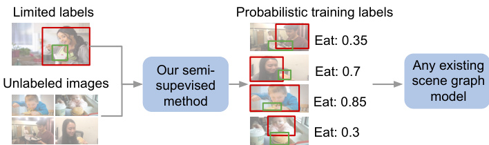
Figure 1. Our semi-supervised method automatically generates probabilistic relationship labels to train any scene graph model.

图 1: 我们的半监督方法自动生成概率关系标签来训练任意场景图模型。

Hiring more human workers is an ineffective solution to labeling relationships because image annotation is so tedious that seemingly obvious labels are left un annotated. To complement human annotators, traditional text-based knowledge completion tasks have leveraged numerous semi-supervised or distant supervision approaches [6, 7, 17, 34]. These methods find syntactical or lexical patterns from a small labeled set to extract missing relationships from a large unlabeled set. In text, pattern-based methods are successful, as relationships in text are usually document-agnostic (e.g. <Tokyo - is capital of - Japan>). Visual relationships are often incidental: they depend on the contents of the particular image they appear in. Therefore, methods that rely on external knowledge or on patterns over concepts (e.g. most instances of dog next to frisbee are playing with it) do not generalize well. The inability to utilize the progress in text-based methods necessitates specialized methods for visual knowledge.

雇佣更多人力标注关系是低效的解决方案，因为图像标注工作极其枯燥，许多看似明显的标签反而未被标注。为辅助人工标注，传统基于文本的知识补全任务已采用大量半监督或远程监督方法 [6, 7, 17, 34]。这些方法通过少量标注数据学习句法或词汇模式，进而从海量未标注数据中提取缺失关系。在文本领域，基于模式的方法成效显著，因为文本关系通常与文档无关（例如<Tokyo - is capital of - Japan>）。而视觉关系往往具有偶发性：其存在取决于所在图像的具体内容。因此，依赖外部知识或概念模式的方法（例如"大多数飞盘旁的狗都在玩耍"）泛化能力较差。由于无法借鉴文本方法的进展，视觉知识领域需要发展专门的方法。

In this paper, we automatically generate missing relationships labels using a small, labeled dataset and use these generated labels to train downstream scene graph models (see Figure 1). We begin by exploring how to define imageagnostic features for relationships so they follow patterns across images. For example, eat usually consists of one object consuming another object smaller than itself, whereas look often consists of common objects: phone, laptop, or window (see Figure 3). These rules are not dependent on raw pixel values; they can be derived from image-agnostic features like object categories and relative spatial positions between objects in a relationship. While such rules are simple, their capacity to provide supervision for un annotated relationships has been unexplored. While image-agnostic features can characterize some visual relationships very well, they might fail to capture complex relationships with high variance. To quantify the efficacy of our image-agnostic features, we define “subtypes” that measure spatial and categorical complexity (Section 3).

本文中，我们利用少量标注数据集自动生成缺失的关系标签，并使用这些生成的标签训练下游场景图模型 (见图 1)。我们首先探索如何定义与图像无关的关系特征，使其能跨图像遵循特定模式。例如，"吃"通常由一个物体消耗另一个比自身小的物体构成，而"看"则常涉及手机、笔记本电脑或窗户等常见物体 (见图 3)。这些规则不依赖于原始像素值，而是源自与图像无关的特征，如物体类别和关系中物体间的相对空间位置。虽然这些规则很简单，但它们为未标注关系提供监督的能力尚未被探索。尽管与图像无关的特征能很好表征某些视觉关系，但可能无法捕捉高方差复杂关系。为量化这些特征的有效性，我们定义了衡量空间和类别复杂度的"子类型" (第3节)。

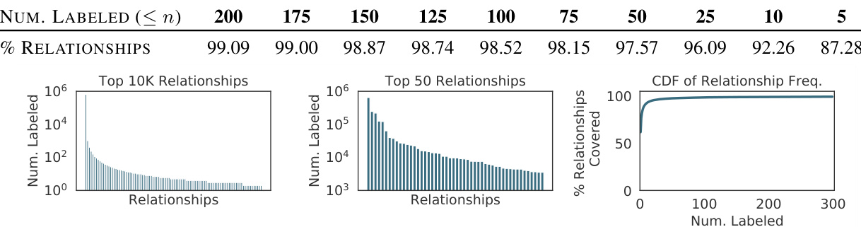
Figure 2. Visual relationships have a long tail (left) of infrequent relationships. Current models [49, 54] only focus on the top 50 relationships (middle) in the Visual Genome dataset, which all have thousands of labeled instances. This ignores more than $98%$ of the relationships with few labeled instances (right, top/table).

图 2: 视觉关系呈现长尾分布(左)，低频关系占多数。现有模型[49, 54]仅关注Visual Genome数据集中标注实例数超千条的前50种关系(中)，忽略了标注实例稀少(右/表)的超过98%的关系类型。

Based on our analysis, we propose a semi-supervised approach that leverages image-agnostic features to label missing relationships using as few as 10 labeled instances of each relationship. We learn simple heuristics over these features and assign probabilistic labels to the unlabeled images using a generative model [39, 46]. We evaluate our method’s labeling efficacy using the completely-labeled VRD dataset [31] and find that it achieves an F1 score of 57.66, which is 11.84 points higher than other standard semi-supervised methods like label propagation [57]. To demonstrate the utility of our generated labels, we train a state-of-the-art scene graph model [54] (see Figure 6) and modify its loss function to support probabilistic labels. Our approach achieves 47.53 recall $@100^{1}$ for predicate classification on Visual Genome, improving over the same model trained using only labeled instances by 40.97 points. For scene graph detection, our approach achieves within 8.65 recall $@100$ of the same model trained on the original Visual Genome dataset with $108\times$ more labeled data. We end by comparing our approach to transfer learning, the de-facto choice for learning from limited labels. We find that our approach improves by 5.16 recall $@100$ for predicate classification, especially for rela tion ships with high complexity, as it generalizes well to unlabeled subtypes.

基于我们的分析，我们提出了一种半监督方法，利用图像无关特征仅需每种关系10个标注实例即可标注缺失关系。我们通过这些特征学习简单启发式规则，并使用生成式模型 [39, 46] 为未标注图像分配概率标签。使用全标注的VRD数据集 [31] 评估标注效能时，本方法F1值达57.66，比标签传播 [57] 等标准半监督方法高出11.84分。为验证生成标签的实用性，我们训练了前沿场景图模型 [54] (见图6)，并修改其损失函数以支持概率标签。在Visual Genome谓词分类任务中，我们的方法实现了47.53的召回率 $@100^{1}$ ，比仅使用标注实例训练的相同模型提升40.97分。场景图检测任务中，本方法召回率 $@100$ 仅比原始Visual Genome数据集(标注数据量多 $108\times$ )训练的相同模型低8.65。最后与迁移学习(有限标签学习的实际选择)对比显示：本方法在谓词分类任务中召回率 $@100$ 提升5.16分，尤其对高复杂度关系效果显著，因其能良好泛化至未标注子类型。

Our contributions are three-fold. (1) We introduce the first method to complete visual knowledge bases by finding missing visual relationships (Section 5.1). (2) We show the utility of our generated labels in training existing scene graph prediction models (Section 5.2). (3) We introduce a metric to characterize the complexity of visual relationships and show it is a strong indicator $:R^{2}=0.778)$ for our semi-supervised method’s improvements over transfer learning (Section 5.3).

我们的贡献有三方面。(1) 我们提出了首个通过发现缺失视觉关系来补全视觉知识库的方法(第5.1节)。(2) 我们展示了生成标签在训练现有场景图预测模型中的实用性(第5.2节)。(3) 我们引入了一个衡量视觉关系复杂度的指标，并证明该指标($:R^{2}=0.778$)能有效预示我们的半监督方法相对于迁移学习的改进效果(第5.3节)。

2. Related work

2. 相关工作

Textual knowledge bases were originally hand-curated by experts to structure facts [4,5,44] (e.g. <Tokyo - capital of - Japan>). To scale dataset curation efforts, recent approaches mine knowledge from the web [9] or hire nonexpert annotators to manually curate knowledge [5, 47]. In semi-supervised solutions, a small amount of labeled text is used to extract and exploit patterns in unlabeled sentences [2, 21, 33–35, 37]. Unfortunately, such approaches cannot be directly applied to visual relationships; textual relations can often be captured by external knowledge or patterns, while visual relationships are often local to an image.

文本知识库最初由专家手工整理以结构化事实 [4,5,44] (例如 <东京 - 首都 - 日本>)。为了扩大数据集整理规模，近期方法从网络挖掘知识 [9] 或雇佣非专业标注员手动整理知识 [5,47]。在半监督解决方案中，少量标注文本被用于提取并利用未标注句子的模式 [2,21,33–35,37]。遗憾的是，这类方法无法直接应用于视觉关系；文本关系通常可通过外部知识或模式捕捉，而视觉关系往往局限于单张图像。

Visual relationships have been studied as spatial priors [14, 16], co-occurrences [51], language statistics [28, 31, 53], and within entity contexts [29]. Scene graph prediction models have dealt with the difficulty of learning from incomplete knowledge, as recent methods utilize statistical motifs [54] or object-relationship dependencies [30, 49, 50, 55]. All these methods limit their inference to the top $50~\mathrm{most}$ frequently occurring predicate categories and ignore those without enough labeled examples (Figure 2).

视觉关系已被研究为空间先验 [14, 16]、共现关系 [51]、语言统计 [28, 31, 53] 以及实体上下文中的关系 [29]。场景图预测模型解决了从不完整知识中学习的难题，近期方法利用了统计模式 [54] 或对象-关系依赖性 [30, 49, 50, 55]。所有这些方法将推理限制在出现频率最高的前 $50~\mathrm{个}$ 谓词类别，并忽略那些缺乏足够标注样本的类别 (图 2)。

The de-facto solution for limited label problems is transfer learning [15, 52], which requires that the source domain used for pre-training follows a similar distribution as the target domain. In our setting, the source domain is a dataset of frequently-labeled relationships with thousands of examples [30, 49, 50, 55], and the target domain is a set of limited label relationships. Despite similar objects in source and target domains, we find that transfer learning has difficulty generalizing to new relationships. Our method does not rely on availability of a larger, labeled set of relationships; instead, we use a small labeled set to annotate the unlabeled set of images.

有限标签问题的实际解决方案是迁移学习 [15, 52]，其要求预训练使用的源域与目标域遵循相似的分布。在我们的设定中，源域是一个包含数千个样本的频繁标注关系数据集 [30, 49, 50, 55]，而目标域是一组有限标签关系。尽管源域和目标域中存在相似对象，但我们发现迁移学习难以泛化到新关系。我们的方法不依赖于更大规模标注关系集的可用性，而是使用少量标注集来对未标注图像集进行注释。

To address the issue of gathering enough training labels for machine learning models, data programming has emerged as a popular paradigm. This approach learns to model imperfect labeling sources in order to assign training labels to unlabeled data. Imperfect labeling sources can come from crowd sourcing [10], user-defined heuristics [8, 43], multi-instance learning [22, 40], and distant supervision [12, 32]. Often, these imperfect labeling sources take advantage of domain expertise from the user. In our case, imperfect labeling sources are automatically generated heuristics, which we aggregate to assign a final probabilistic label to every pair of object proposals.

为解决机器学习模型获取足够训练标签的问题，数据编程已成为一种流行范式。该方法通过学习建模不完美标注源，从而为未标注数据分配训练标签。不完美标注源可来自众包 [10]、用户自定义启发式规则 [8, 43]、多示例学习 [22, 40] 以及远程监督 [12, 32]。这些不完美标注源通常利用了用户的领域专业知识。在我们的案例中，不完美标注源是自动生成的启发式规则，我们通过聚合这些规则为每对对象提案分配最终的概率标签。

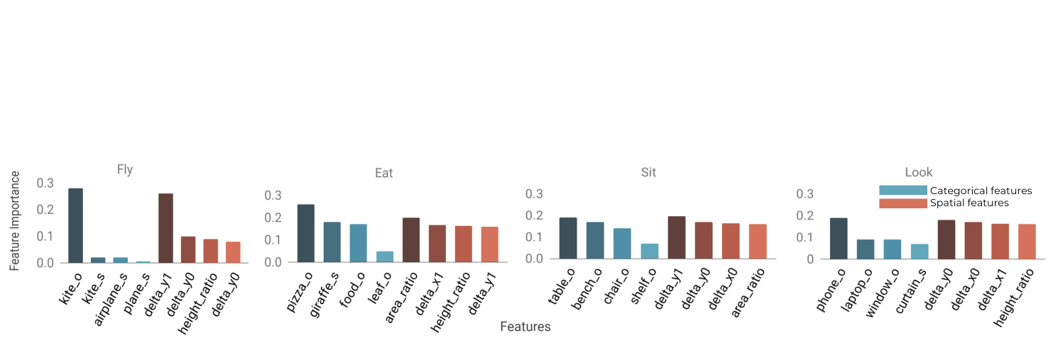
Figure 3. Relationships, such as fly, eat, and sit can be characterized effectively by their categorical (s and $\bigcirc$ refer to subject and object, respectively) or spatial features. Some relationships like fly rely heavily only on a few features — kites are often seen high up in the sky.

图 3: 诸如飞翔、进食、坐下等关系可通过其类别特征 (s 和 $\bigcirc$ 分别表示主体和客体) 或空间特征有效表征。某些关系 (如飞翔) 往往仅依赖少数特征——风筝通常出现在高空。

3. Analyzing visual relationships

3. 分析视觉关系

We define the formal terminology used in the rest of the paper and introduce the image-agnostic features that our semi-supervised method relies on. Then, we seek quantitative insights into how visual relationships can be described by the properties between its objects. We ask (1) what imageagnostic features can characterize visual relationships? and (2) given limited labels, how well do our chosen features characterize the complexity of relationships? With these in mind, we motivate our model design to generate heuristics that do not overfit to the small amount of labeled data and assign accurate labels to the larger, unlabeled set.

我们定义了本文其余部分使用的正式术语，并介绍了半监督方法所依赖的图像无关特征。接着，我们定量探究了视觉关系如何通过其对象间的属性进行描述。我们提出两个问题：(1) 哪些图像无关特征能表征视觉关系？(2) 在有限标注条件下，所选特征对关系复杂度的表征效果如何？基于此，我们设计了能够避免对小规模标注数据过拟合的启发式模型，旨在为更大规模的无标注数据集分配准确标签。

3.1. Terminology

3.1. 术语

A scene graph is a multi-graph $\mathbb{G}$ that consists of objects $o$ as nodes and relationships $r$ as edges. Each object $o_{i}=$ ${b_{i},c_{i}}$ consists of a bounding box $b_{i}$ and its category $c_{i}\in$ $\mathbb{C}$ where $\mathbb{C}$ is the set of all possible object categories (e.g. dog, frisbee). Relationships are denoted <subject - predicate - object> or ${<}o\mathrm{ -~}p\mathrm{ -~}o^{\prime}{>}$ . $p\in\mathbb{P}$ is a predicate, such as ride and eat. We assume that we have a small labeled set ${(o,p,o^{\prime})\in D_{p}}$ of annotated relationships for each predicate $p$ . Usually, these datasets are on the order of a 10 examples or fewer. For our semisupervised approach, we also assume that there exists a large set of images $D_{U}$ without any labeled relationships.

场景图是一种多图 $\mathbb{G}$，由作为节点的物体 $o$ 和作为边的关系 $r$ 组成。每个物体 $o_{i}=$ ${b_{i},c_{i}}$ 包含一个边界框 $b_{i}$ 及其类别 $c_{i}\in$ $\mathbb{C}$，其中 $\mathbb{C}$ 是所有可能的物体类别集合（例如狗、飞盘）。关系表示为<主体-谓词-客体>或 ${<}o\mathrm{ -~}p\mathrm{ -~}o^{\prime}{>}$。$p\in\mathbb{P}$ 是谓词，例如骑和吃。我们假设对于每个谓词 $p$，有一个带标注关系的小型标注集 ${(o,p,o^{\prime})\in D_{p}}$。通常，这些数据集的规模约为10个或更少的样本。对于我们的半监督方法，我们还假设存在一个没有任何标注关系的大型图像集 $D_{U}$。

3.2. Defining image-agnostic features

3.2. 定义与图像无关的特征

It has become common in computer vision to utilize pretrained convolutional neural networks to extract features that represent objects and visual relationships [31, 49, 50]. Models trained with these features have proven robust in the presence of enough training labels but tend to overfit when presented with limited data (Section 5). Consequently, an open question arises: what other features can we utilize to label relationships with limited data? Previous literature has combined deep learning features with extra information extracted from categorical object labels and relative spatial object locations [25, 31]. We define categorical features, $<o,-,o^{\prime}>$ , as a concatenation of one-hot vectors of the subject $o$ and object $o^{\prime}$ . We define spatial features as:

在计算机视觉领域，利用预训练的卷积神经网络提取表征物体及视觉关系的特征已成为常见做法 [31, 49, 50]。使用这些特征训练的模型在具备充足训练标签时表现稳健，但在数据有限时容易过拟合 (第5节)。这引出一个开放性问题：面对有限数据，我们还能利用哪些特征来标注关系？已有研究将深度学习特征与从类别物体标签及相对空间位置提取的额外信息相结合 [25, 31]。我们将类别特征 $<o,-,o^{\prime}>$ 定义为主体 $o$ 和客体 $o^{\prime}$ 的独热向量拼接，空间特征定义为：

$$
\begin{array}{r l r}{\displaystyle\frac{x-x^{\prime}}{w},\displaystyle\frac{y-y^{\prime}}{h},\displaystyle\frac{(y+h)-(y^{\prime}+h^{\prime})}{h},}&{{}}&{}\ {\displaystyle\frac{(x+w)-(x^{\prime}+w^{\prime})}{w},\displaystyle\frac{h^{\prime}}{h},\displaystyle\frac{w^{\prime}}{w},\displaystyle\frac{w^{\prime}h^{\prime}}{w h},\displaystyle\frac{w^{\prime}+h^{\prime}}{w+h}}&{{}}&{}\end{array}
$$

$$
\begin{array}{r l r}{\displaystyle\frac{x-x^{\prime}}{w},\displaystyle\frac{y-y^{\prime}}{h},\displaystyle\frac{(y+h)-(y^{\prime}+h^{\prime})}{h},}&{{}}&{}\ {\displaystyle\frac{(x+w)-(x^{\prime}+w^{\prime})}{w},\displaystyle\frac{h^{\prime}}{h},\displaystyle\frac{w^{\prime}}{w},\displaystyle\frac{w^{\prime}h^{\prime}}{w h},\displaystyle\frac{w^{\prime}+h^{\prime}}{w+h}}&{{}}&{}\end{array}
$$

where $b=[{y},{x},{h},{w}]$ and $b^{\prime}=[y^{\prime},x^{\prime},h^{\prime},w^{\prime}]$ are the topleft bounding box coordinates and their widths and heights.

其中 $b=[{y},{x},{h},{w}]$ 和 $b^{\prime}=[y^{\prime},x^{\prime},h^{\prime},w^{\prime}]$ 分别是左上角边界框坐标及其宽度和高度。

To explore how well spatial and categorical features can describe different visual relationships, we train a simple decision tree model for each relationship. We plot the importances for the top 4 spatial and categorical features in Figure 3. Relationships like $\tt f l y$ place high importance on the difference in y-coordinate between the subject and object, capturing a characteristic spatial pattern. look, on the other hand, depends on the category of the objects (e.g. phone, laptop, window) and not on any spatial orientations.

为了探究空间和类别特征在描述不同视觉关系时的表现，我们为每种关系训练了一个简单的决策树模型。图3展示了前4位空间和类别特征的重要性排序。像$\tt f l y$这类关系高度依赖主体与客体之间的y坐标差值，这捕捉到了特定的空间模式。而look则取决于物体类别(如phone、laptop、window)，与空间方位无关。

3.3. Complexity of relationships

3.3. 关系复杂性

To understand the efficacy of image-agnostic features, we’d like to measure how well they can characterize the complexity of particular visual relationships. As seen in Figure 4, a visual relationship can be defined by a number of image-agnostic features (e.g. a person can ride a bike, or a dog can ride a surfboard). To systematically define this notion of complexity, we identify subtypes for each visual relationship. Each subtype captures one way that a relationship manifests in the dataset. For example, in Figure 4, ride contains one categorical subtype with <person - ride - bike> and another with <dog - ride - surfboard>. Similarly, a person might carry an object in different relative spatial orientations (e.g. on her head, to her side). As shown in Figure 5, visual relationships might have significantly different degrees of spatial and categorical complexity, and therefore a different number of subtypes for each. To compute spatial subtypes, we perform mean shift clustering [11] over the spatial features extracted from all the relationships in Visual Genome. To compute the categorical subtypes, we count the number of unique object categories associated with a relationship.

为了理解图像无关特征的有效性，我们希望能衡量它们对特定视觉关系复杂度的表征能力。如图4所示，一个视觉关系可以通过多个图像无关特征来定义（例如人可以骑自行车，或狗可以冲浪板）。为了系统化定义这种复杂度概念，我们为每个视觉关系识别了子类型。每个子类型捕捉了该关系在数据集中呈现的一种方式。例如在图4中，"骑"包含一个分类子类型<人-骑-自行车>和另一个<狗-骑-冲浪板>。类似地，一个人可能以不同的相对空间方位携带物体（例如头顶、身侧）。如图5所示，视觉关系可能在空间和分类复杂度上存在显著差异，因此每个关系的子类型数量也不同。为计算空间子类型，我们对Visual Genome中所有关系提取的空间特征执行均值漂移聚类[11]。为计算分类子类型，我们统计与每个关系相关联的唯一物体类别数量。

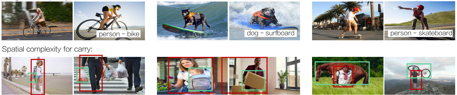
Figure 4. We define the number of subtypes of a relationship as a measure of its complexity. Subtypes can be categorical — one subtype of ride can be expressed as <person - ride - bike> while another is <dog - ride - surfboard>. Subtypes can also be spatial — carry has a subtype with a small object carried to the side and another with a large object carried overhead.

图 4: 我们将关系的子类型数量定义为其复杂性的衡量标准。子类型可以是类别性的——例如"骑乘"关系的一个子类型可表示为<人-骑-自行车>，而另一个子类型是<狗-骑-冲浪板>。子类型也可以是空间性的——例如"携带"关系存在一个子类型是小物体侧身携带，另一个子类型是大物体举过头顶携带。

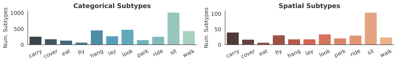
Figure 5. A subset of visual relationships with different levels of complexity as defined by spatial and categorical subtypes. In Section 5.3, we show how this measure is a good indicator of our semi-supervised method’s effectiveness compared to baselines like transfer learning.

图 5: 按空间和类别子类型划分的不同复杂度视觉关系子集。在第 5.3 节中，我们将展示相较于迁移学习等基线方法，该衡量标准如何有效体现我们半监督方法的优越性。

With access to 10 or fewer labeled instances for these visual relationships, it is impossible to capture all the subtypes for given relationship and therefore difficult to learn a good representation for the relationship as a whole. Consequently, we turn to the rules extracted from image-agnostic features and use them to assign labels to the unlabeled data in order to capture a larger proportion of subtypes in each visual relationship. We posit that this will be advantageous over methods that only use the small labeled set to train a scene graph prediction model, especially for relationships with high complexity, or a large number of subtypes. In Section 5.3, we find a correlation between our definition of complexity and the performance of our method.

在仅能获取10个或更少标注实例的情况下，这些视觉关系无法涵盖给定关系的所有子类型，因此难以学习到该关系的整体良好表征。为此，我们转向从图像无关特征中提取规则，并利用这些规则为未标注数据分配标签，以捕获每个视觉关系中更大比例的子类型。我们认为，这种方法将优于仅使用少量标注集训练场景图预测模型的方法，特别是对于具有高复杂性或大量子类型的关系。在第5.3节中，我们发现所定义的复杂性与方法性能之间存在相关性。

4. Approach

4. 方法

We aim to automatically generate labels for missing visual relationships that can be then used to train any downstream scene graph prediction model. We assume that in the longtail of infrequent relationships, we have a small labeled set ${(o,p,o^{\prime})\in D_{p}}$ of annotated relationships for each predicate $p$ (often, on the order of a 10 examples or less). As discussed in Section 3, we want to leverage image-agnostic features to learn rules that annotate unlabeled relationships.

我们的目标是自动为缺失的视觉关系生成标签，这些标签随后可用于训练任何下游场景图预测模型。我们假设在低频关系的长尾分布中，对于每个谓词 $p$ ，我们有一个带标注关系的小型标注集 ${(o,p,o^{\prime})\in D_{p}}$ （通常约为10个或更少的示例）。如第3节所述，我们希望利用与图像无关的特征来学习标注未标记关系的规则。

Our approach assigns probabilistic labels to a set $D_{U}$ of un-annotated images in three steps: (1) we extract imageagnostic features from the objects in the labeled $D_{p}$ and

我们的方法通过三个步骤为一组未标注图像 $D_{U}$ 分配概率标签：(1) 从标注集 $D_{p}$ 中的对象提取与图像无关的特征，

Algorithm 1 Semi-supervised Alg. to Label Relationships

算法 1: 半监督关系标注算法

from the object proposals extracted using an existing object detector [19] on unlabeled $D_{U}$ , (2) we generate heuristics over the image-agnostic features, and finally (3) we use a factor-graph based generative model to aggregate and assign probabilistic labels to the unlabeled object pairs in $D_{U}$ . These probabilistic labels, along with $D_{p}$ , are used to train any scene graph prediction model. We describe our approach in Algorithm 1 and show the end-to-end pipeline in Figure 6. Feature extraction: Our approach uses the image-agnostic features defined in Section 3, which rely on object bounding box and category labels. The features are extracted from ground truth objects in $D_{p}$ or from object detection outputs in $D_{U}$ by running existing object detection models [19].

从使用现有物体检测器[19]在未标记的$D_{U}$上提取的物体提案中，(1) 我们基于图像无关特征生成启发式规则，(2) 最后(3) 我们使用基于因子图的生成模型来聚合并为$D_{U}$中未标记的物体对分配概率标签。这些概率标签与$D_{p}$一起用于训练任何场景图预测模型。我们在算法1中描述了我们的方法，并在图6中展示了端到端流程。特征提取：我们的方法使用了第3节中定义的图像无关特征，这些特征依赖于物体边界框和类别标签。特征通过运行现有物体检测模型[19]，从$D_{p}$中的真实物体或$D_{U}$中的物体检测输出中提取。

Heuristic generation: We fit decision trees over the labeled relationships’ spatial and categorical features to capture image-agnostic rules that define a relationship. These image-agnostic rules are threshold-based conditions that are automatically defined by the decision tree. To limit the complexity of these heuristics and thereby prevent over fitting, we use shallow decision trees [38] with different restrictions on depth over each feature set to produce $J$ different decision trees. We then predict labels for the unlabeled set using these heuristics, producing a $\boldsymbol{\Lambda}\in\mathbb{R}^{J\times|D_{U}|}$ matrix of predictions for the unlabeled relationships.

启发式生成：我们基于已标注关系的空间和类别特征拟合决策树，以捕捉定义关系的图像无关规则。这些图像无关规则是由决策树自动定义的基于阈值的条件。为了限制这些启发式规则的复杂度从而防止过拟合，我们使用浅层决策树 [38]，对每个特征集施加不同的深度限制，生成 $J$ 棵不同的决策树。随后，我们利用这些启发式规则对未标注集进行标签预测，生成一个未标注关系的预测矩阵 $\boldsymbol{\Lambda}\in\mathbb{R}^{J\times|D_{U}|}$。

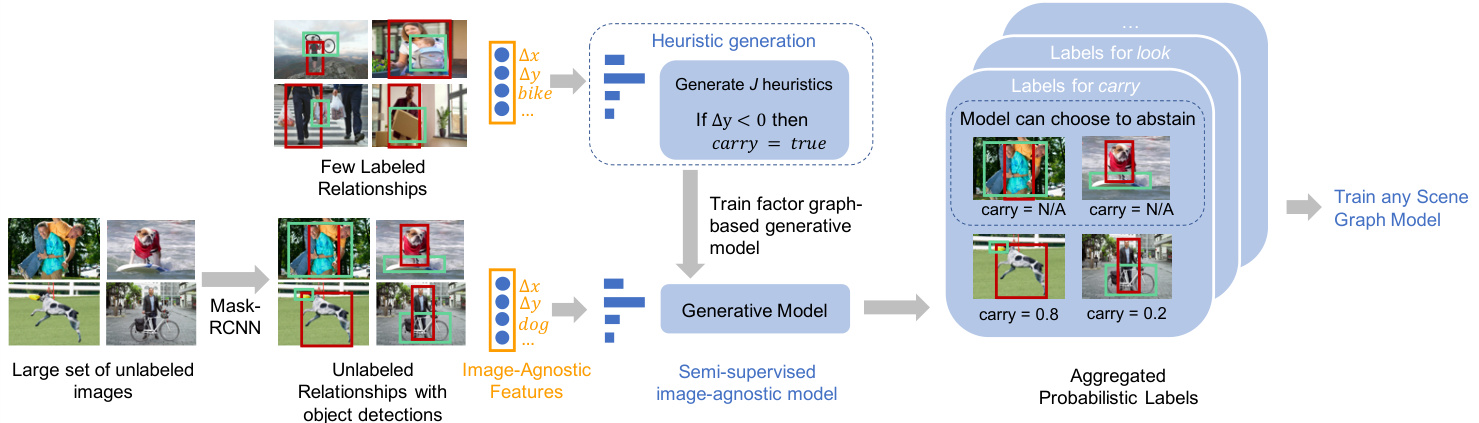
Figure 6. For a relationship (e.g., carry), we use image-agnostic features to automatically create heuristics and then use a generative model to assign probabilistic labels to a large unlabeled set of images. These labels can then be used to train any scene graph prediction model.

图 6: 对于某种关系(如carry), 我们使用与图像无关的特征自动创建启发式规则, 然后通过生成式模型为大量未标注图像分配概率标签。这些标签可用于训练任何场景图预测模型。

Moreover, we only use these heuristics when they have high confidence about their label; we modify $\Lambda$ by converting any predicted label with confidence less than a threshold (empirically chosen to be $2\times$ random) to an abstain, or no label assignment. An example of a heuristic is shown in Figure 6: if the subject is above the object, it assigns a positive label for the predicate carry.

此外，我们仅在启发式规则对其标签具有高置信度时才会使用它们；我们通过将所有置信度低于阈值（经验性选择为随机值的2倍）的预测标签转换为弃权（即不分配标签）来修改$\Lambda$。图6展示了一个启发式规则的示例：如果主体位于客体上方，则为谓词carry分配正标签。

Generative model: These heuristics, individually, are noisy and may not assign labels to all object pairs in $D_{U}$ . As a result, we aggregate the labels from all $J$ heuristics. To do so, we leverage a factor graph-based generative model popular in text-based weak supervision techniques [1, 39, 41, 45, 48]. This model learns the accuracies of each heuristic to combine their individual labels; the model’s output is a probabilistic label for each object pair.

生成式模型 (Generative model): 这些启发式方法单独使用时存在噪声, 可能无法为 $D_{U}$ 中的所有对象对分配标签。因此, 我们聚合了所有 $J$ 个启发式方法的标签。为此, 我们采用了基于因子图的生成模型, 该模型在基于文本的弱监督技术中广泛应用 [1, 39, 41, 45, 48]。该模型通过学习每个启发式方法的准确率来整合它们的个体标签, 最终为每个对象对输出一个概率标签。

The generative model $G$ uses the following distribution family to relate the latent variable $Y\in\mathbb{R}^{|D_{U}|}$ , the true class, and the labels from the heuristics, $\Lambda$ :

生成模型 $G$ 使用以下分布族来关联潜在变量 $Y\in\mathbb{R}^{|D_{U}|}$ 、真实类别以及来自启发式的标签 $\Lambda$：

$$
\pi_{\phi}(\Lambda,Y)=\frac{1}{Z_{\phi}}\exp\left(\phi^{T}\Lambda Y\right)
$$

$$
\pi_{\phi}(\Lambda,Y)=\frac{1}{Z_{\phi}}\exp\left(\phi^{T}\Lambda Y\right)
$$

where $Z_{\phi}$ is a partition function to ensure $\pi$ is normalized. The parameter $\phi\in\mathbb{R}^{J}$ encodes the average accuracy of each heuristic and is estimated by maximizing the marginal likelihood of the observed heuristic $\Lambda$ . The generative model assigns probabilistic labels by computing $\pi_{\phi}(Y\mid\Lambda(o,o^{\prime}))$ for each object pair $(o,o^{\prime})$ in $D_{U}$ .

其中 $Z_{\phi}$ 是确保 $\pi$ 归一化的配分函数。参数 $\phi\in\mathbb{R}^{J}$ 编码了每个启发式的平均准确率，并通过最大化观测到的启发式 $\Lambda$ 的边际似然来估计。该生成模型通过为 $D_{U}$ 中的每个对象对 $(o,o^{\prime})$ 计算 $\pi_{\phi}(Y\mid\Lambda(o,o^{\prime}))$ 来分配概率标签。

Training scene graph model: Finally, these probabilistic labels are used to train any scene graph prediction model. While scene graph models are usually trained using a crossentropy loss [31, 49, 54], we modify this loss function to take into account errors in the training annotations. We adopt a noise-aware empirical risk minimizer that is often seen in logistic regression as our loss function:

训练场景图模型：最后，这些概率标签被用于训练任何场景图预测模型。虽然场景图模型通常使用交叉熵损失函数进行训练 [31, 49, 54]，但我们修改了这一损失函数以考虑训练标注中的错误。我们采用了一种在逻辑回归中常见的噪声感知经验风险最小化器作为损失函数：

Table 1. We validate our approach for labeling missing relationships using only $n=10$ labeled examples by evaluating our probabilistic labels from our semi-supervised approach over the fully-annotated VRD using macro metrics dataset [31].

表 1: 我们仅使用 $n=10$ 个标注样本验证了缺失关系标注方法，通过在完整标注的VRD数据集上使用宏观指标 [31] 评估半监督方法生成的概率标签。

模型 (n = 10)	精确率	召回率	F1值	准确率
RANDOM	5.00	5.00	5.00	5.00
DECISIONTREE	46.79	35.32	40.25	36.92
LABELPROPAGATION	76.48	32.71	45.82	12.85
OURS (MAJORITYVOTE)	55.01	57.26	56.11	40.04
OURS (CATEG.+ SPAT.)	54.83	60.79	57.66	50.31

$$
L_{\theta}=\mathbb{E}_{Y\sim\pi}\left[\log\left(1+\exp(-\theta^{T}V^{T}Y)\right)\right]
$$

$$
L_{\theta}=\mathbb{E}_{Y\sim\pi}\left[\log\left(1+\exp(-\theta^{T}V^{T}Y)\right)\right]
$$

where $\theta$ is the learned parameters, $\pi$ is the distribution learned by the generative model, $Y$ is the true label, and $V$ are features extracted by any scene graph prediction model.

其中 $\theta$ 是学习到的参数，$\pi$ 是生成式模型学习到的分布，$Y$ 是真实标签，$V$ 是由任意场景图预测模型提取的特征。

5. Experiments

5. 实验

To test our semi-supervised approach for completing visual knowledge bases by annotating missing relationships, we perform a series of experiments and evaluate our framework in several stages. We start by discussing the datasets, baselines, and evaluation metrics used. (1) Our first experiment tests our generative model’s ability to find missing relationships in the completely-annotated VRD dataset [31]. (2) Our second experiment demonstrates the utility of our generated labels by using them to train a state-of-the-art scene graph model [54]. We compare our labels to those from the large Visual Genome dataset [27]. (3) Finally, to show that our semi-supervised method’s performance compared to strong baselines in limited label settings, we compare extensively to transfer learning; we focus on a subset of relationships with limited labels, allow the transfer learning model to pretrain on frequent relationships, and demonstrate that our semi-supervised method outperforms transfer learning, which has seen more data. Furthermore, we quantify when our method outperforms transfer learning using our metric for measuring relationship complexity (Section 3.3).

为了测试我们通过标注缺失关系来补全视觉知识库的半监督方法，我们进行了一系列实验，并分阶段评估了我们的框架。首先讨论使用的数据集、基线方法和评估指标。(1) 第一个实验测试了我们的生成模型在完全标注的VRD数据集[31]中发现缺失关系的能力。(2) 第二个实验通过使用生成的标签训练最先进的场景图模型[54]，展示了生成标签的实用性。我们将生成的标签与大型Visual Genome数据集[27]中的标签进行了比较。(3) 最后，为了展示在有限标签设置下我们的半监督方法相较于强基线的性能，我们与迁移学习进行了广泛比较；我们聚焦于标签有限的关系子集，允许迁移学习模型在频繁关系上进行预训练，并证明我们的半监督方法优于接触过更多数据的迁移学习。此外，我们使用衡量关系复杂度的指标(第3.3节)量化了我们的方法何时优于迁移学习。

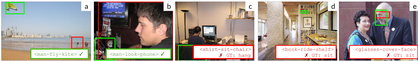
Figure 7. (a) Heuristics based on spatial features help predict <man - fly - kite>. (b) Our model learns that look is highly correlated with phone. (c) We overfit to the importance of chair as a categorical feature for sit, and fail to identify hang as the correct relationship. (d) We overfit to the spatial positioning associated with ride, where objects are typically longer and directly underneath the subject. (e) Given our image-agnostic features, we produce a reasonable label for <glass - cover - face>. However, our model is incorrect, as two typically different predicates (sit and cover) share a semantic meaning in the context of <glasses - ? - face>.

图 7: (a) 基于空间特征的启发式方法有助于预测<人 - 放 - 风筝>。(b) 我们的模型学习到"看"与"手机"高度相关。(c) 我们对"sit"的类别特征"椅子"的重要性过拟合，未能识别"hang"才是正确关系。(d) 我们对"ride"相关的空间定位过拟合，该场景中物体通常更长且直接位于主体下方。(e) 由于采用图像无关特征，我们为<眼镜 - ? - 脸>生成合理标签。但模型实际是错误的，因为两个通常不同的谓词(sit和cover)在<眼镜 - ? - 脸>语境下具有相同语义。

Eliminating synonyms and supersets. Typically, past scene graph approaches have used 50 predicates from Visual Genome to study visual relationships. Unfortunately, these 50 treat synonyms like laying on and lying on as separate classes. To make matters worse, some predicates can be considered a superset of others (i.e. above is a superset of riding). Our method, as well as the baselines, is unable to differentiate between synonyms and supersets. For the experiments in this section, we eliminate all supersets and merge all synonyms, resulting in 20 unique predicates. In the Appendix (A1) we include a list of these predicates and report our method’s performance on all 50 predicates.

消除同义词和超集。通常，过去的场景图方法使用Visual Genome中的50个谓词来研究视觉关系。遗憾的是，这50个谓词将同义词（如laying on和lying on）视为不同类别。更糟糕的是，某些谓词可被视为其他谓词的超集（例如above是riding的超集）。我们的方法及基线模型均无法区分同义词和超集。在本节实验中，我们剔除了所有超集并合并同义词，最终得到20个唯一谓词。附录(A1)列出了这些谓词，并报告了我们的方法在全部50个谓词上的性能表现。

Dataset. We use two standard datasets, VRD [31] and Visual Genome [27], to evaluate on tasks related to visual relationships or scene graphs. Each scene graph contains objects localized as bounding boxes in the image along with pairwise relationships connecting them, categorized as action (e.g., carry), possessive (e.g., wear), spatial (e.g., above), or comparative (e.g., taller than) descriptors. Visual Genome is a large visual knowledge base containing $108K$ images. Due to its scale, each scene graph is left with incomplete labels, making it difficult to measure the precision of our semi-supervised algorithm. VRD is a smaller but completely annotated dataset. To show the performance of our semi-supervised method, we measure our method’s generated labels on the VRD dataset (Section 5.1). Later, we show that the training labels produced can be used to train a large scale scene graph prediction model, evaluated on Visual Genome (Section 5.2).

数据集。我们使用两个标准数据集 VRD [31] 和 Visual Genome [27] 来评估与视觉关系或场景图相关的任务。每个场景图包含以图像中边界框定位的对象，以及连接它们的成对关系，这些关系被分类为动作 (如 carry) 、所属 (如 wear) 、空间 (如 above) 或比较 (如 taller than) 描述符。Visual Genome 是一个大型视觉知识库，包含 $108K$ 张图像。由于其规模，每个场景图都留有未完成的标签，这使得难以衡量我们半监督算法的精度。VRD 是一个较小但完全标注的数据集。为了展示我们半监督方法的性能，我们在 VRD 数据集上测量了方法生成的标签 (第 5.1 节)。随后，我们展示了生成的训练标签可用于训练大规模场景图预测模型，并在 Visual Genome 上进行评估 (第 5.2 节)。

Evaluation metrics. We measure precision and recall of our generated labels on the VRD dataset’s test set (Section 5.1). To evaluate a scene graph model trained on our labels, we use three standard evaluation modes for scene graph prediction [31]: (i) scene graph detection (SGDET) which expects input images and predicts bounding box locations, object categories, and predicate labels, (ii) scene graph classification (SGCLS) which expects ground truth boxes and predicts object categories and predicate labels, and (iii) predicate classification (PREDCLS), which expects ground truth bounding boxes and object categories to predict predicate labels. We refer the reader to the paper that introduced these tasks for more details [31]. Finally, we explore how relationship complexity, measured using our definition of subtypes, is correlated with our model’s performance relative to transfer learning (Section 5.3).

评估指标。我们在VRD数据集的测试集上测量生成标签的精确率和召回率（第5.1节）。为了评估基于我们标签训练的场景图模型，我们采用三种标准场景图预测评估模式[31]：(i) 场景图检测(SGDET)，要求输入图像并预测边界框位置、物体类别和谓词标签；(ii) 场景图分类(SGCLS)，要求真实标注框并预测物体类别和谓词标签；(iii) 谓词分类(PREDCLS)，要求真实边界框和物体类别来预测谓词标签。详细说明请参阅提出这些任务的论文[31]。最后，我们探讨了使用子类型定义衡量的关系复杂度与模型在迁移学习中的性能相关性（第5.3节）。

Baselines. We compare to alternative methods for generating training labels that can then be used to train downstream scene graph models. ORACLE is trained on all of Visual Genome, which amounts to $108\times$ the quantity of labeled relationships in $D_{p}$ ; this serves as the upper bound for how well we expect to perform. DECISION TREE [38] fits a single decision tree over the image-agnostic features, learns from labeled examples in $D_{p}$ , and assigns labels to $D_{U}$ . LABEL PROPAGATION [57] employs a widely-used semi-supervised method and considers the distribution of image-agnostic features in $D_{U}$ before propagating labels from $D_{p}$ to $D_{U}$ .

基线方法。我们与其他生成训练标签的方法进行比较，这些标签可用于训练下游场景图模型。ORACLE在完整的Visual Genome数据集上训练，其标注关系数量是$D_{p}$的$108\times$倍，这代表了性能上限。DECISION TREE [38]基于图像无关特征拟合单一决策树，通过$D_{p}$的标注样本学习后为$D_{U}$分配标签。LABEL PROPAGATION [57]采用广泛使用的半监督方法，在将$D_{p}$的标签传播至$D_{U}$前会考虑$D_{U}$中图像无关特征的分布。

We compare to a strong frequency baselines: (FREQ) uses the object counts as priors to make relationship predictions, and FREQ $+$ OVERLAP increments such counts only if the bounding boxes of objects overlap. We include a TRANSFER LEARNING baseline, which is the de-facto choice for training models with limited data [15, 52]. However, unlike all other methods, transfer learning requires a source dataset to pretrain. We treat the source domain as the remaining relationships from the top 50 in Visual Genome that do not overlap with our chosen relationships. We then fine tune with the limited labeled examples for the predicates in $D_{p}$ . We note that TRANSFER LEARNING has an unfair advantage because there is overlap in objects between its source and target relationship sets. Our experiments will show that even with this advantage, our method performs better.

我们与一个强大的频率基线进行比较：(FREQ) 使用物体计数作为先验来预测关系，而 FREQ $+$ OVERLAP 仅在物体边界框重叠时增加计数。我们还包含了一个迁移学习 (TRANSFER LEARNING) 基线，这是在数据有限时训练模型的实际选择 [15, 52]。然而，与所有其他方法不同，迁移学习需要一个源数据集进行预训练。我们将源域视为 Visual Genome 中前 50 个关系中未与我们选定关系重叠的部分，然后在 $D_{p}$ 的有限标注示例上对谓词进行微调。需要注意的是，迁移学习具有不公平的优势，因为其源和目标关系集之间存在物体重叠。我们的实验将表明，即使存在这一优势，我们的方法表现更优。

Ablations. We perform several ablation studies for the image-agnostic features and heuristic aggregation components of our model. (CATEG.) uses only categorical features, (SPAT.) uses only spatial features, (DEEP) uses only deep learning features extracted using ResNet50 [20] from the union of the object pair’s bounding boxes, (CATEG. $+\mathrm{SPAT}.$ .) uses both categorical concatenated with spatial features, (CATEG. $^+$ SPAT. $^+$ DEEP) combines combines all three, and OURS (CATEG. $+\mathrm{SPAT}$ . $^+$ WORDVEC) includes word vectors as richer representations of the categorical features. (MAJORITY VOTE) uses the categorical and spatial features but replaces our generative model with a simple majority voting scheme to aggregate heuristic function outputs.

消融实验。我们对模型中与图像无关的特征和启发式聚合组件进行了多项消融研究：(CATEG.)仅使用类别特征，(SPAT.)仅使用空间特征，(DEEP)仅使用通过ResNet50[20]从物体对边界框并集提取的深度学习特征，(CATEG. $+\mathrm{SPAT}.$ .)同时使用类别特征和空间特征并将它们拼接，(CATEG. $^+$ SPAT. $^+$ DEEP)结合了所有三种特征，而OURS (CATEG. $+\mathrm{SPAT}$ . $^+$ WORDVEC)在基础上加入了词向量作为类别特征的更丰富表示。(MAJORITY VOTE)使用类别和空间特征，但用简单的多数投票方案替代我们的生成模型来聚合启发式函数输出。

Table 2. Results for scene graph prediction tasks with $n=10$ labeled examples per predicate, reported as recall $\ @\mathrm{K}$ . A state-of-the-art scene graph model trained on labels from our method outperforms those trained with labels generated by other baselines, like transfer learning.

表 2: 每个谓词使用 $n=10$ 个标注样本的场景图预测任务结果 (以召回率 $\ @\mathrm{K}$ 报告) 。采用本方法标注数据训练的最新场景图模型，其性能优于迁移学习等其他基线方法生成的标注数据训练的模型。

模型	场景图检测 R@20	R@50	R@100	场景图分类 R@20	R@50	R@100	谓词分类 R@20	R@50	R@100
BASELINE [n = 10]	0.00	0.00	0.00	0.04	0.04	0.04	3.17	5.30	6.61
FREQ	9.01	11.01	11.64	11.10	11.08	10.92	20.98	20.98	20.80
FREQ+OVERLAP	10.16	10.84	10.86	9.90	9.91	9.91	20.39	20.90	22.21
TRANSFERLEARNING	11.99	14.40	16.48	17.10	17.91	18.16	39.69	41.65	42.37
B DECISION TREE[38]	11.11	12.58	13.23	14.02	14.51	14.57	31.75	33.02	33.35
LABEL PROPAGATION[57]	6.48	6.74	6.83	9.67	9.91	9.97	24.28	25.17	25.41
OURS (DEEP)	2.97	3.20	3.33	10.44	10.77	10.84	23.16	23.93	24.17
OURS (SPAT.)	3.26	3.20	2.91	10.98	11.28	11.37	26.23	27.10	27.26
OURS (CATEG.)	7.57	7.92	8.04	20.83	21.44	21.57	43.49	44.93	45.50
OURS (CATEG.+ SPAT.+ DEEP)	7.33	7.70	7.79	17.03	17.35	17.39	38.90	39.87	40.02
OURS (CATEG.+ SPAT.+ WORDVEC)	8.43	9.04	9.27	20.39	20.90	21.21	45.15	46.82	47.32
OURS (MAJORITYVOTE)	16.86	18.31	18.57	18.96	19.57	19.66	44.18	45.99	46.63
OURS (CATEG. + SPAT.)	17.67	18.69	19.28	20.91	21.34	21.44	45.49	47.04	47.53
ORACLE [NoRACLE = 108n]	24.42	29.67	30.15	30.15	30.89	31.09	69.23	71.40	72.15

增加标注数据的影响
增加未标注数据的影响

场景图分类 30	谓词分类	场景图分类 75 50	谓词分类
80	60 Oracle	0 30
20	40 Ours	20
	Transfer		25 suno
10	20 Baseline	0	Oracle
0 0	0 0 100 200 Num. Labeled	0 10000 20000 Num. Unlabeled	0 0 10000 20000 Num.Unlabeled

Figure 8. A scene graph model [54] trained using our labels outperforms both using TRANSFER LEARNING labels and using only the BASELINE labeled examples consistently across scene graph classification and predicate classification for different amounts of available labeled relationship instances. We also compare to ORACLE, which is trained with $108\times$ more labeled data.

图 8: 使用我们标注数据训练的场景图模型 [54] 在不同数量的可用标注关系实例下，于场景图分类和谓词分类任务中均持续优于使用迁移学习 (TRANSFER LEARNING) 标注数据和仅使用基线 (BASELINE) 标注样本的方法。我们还对比了使用 $108\times$ 更多标注数据训练的 ORACLE 模型。

5.1. Labeling missing relationships

5.1. 缺失关系标注

We evaluate our performance in annotating missing rela tion ships in $D_{U}$ . Before we use these labels to train scene graph prediction models, we report results comparing our method to baselines in Table 1. On the fully annotated VRD dataset [31], OURS (CATEG. $+\mathrm{SPAT}.$ ) achieves 57.66 F1 given only 10 labeled examples, which is 17.41, 13.88, and 1.55 points better than LABEL PROPAGATION, DECISION TREE and MAJORITY VOTE, respectively.

我们评估了在$D_{U}$中标注缺失关系的性能。在使用这些标签训练场景图预测模型之前，我们在表1中报告了与基线方法的对比结果。在完全标注的VRD数据集[31]上，OURS (CATEG. $+\mathrm{SPAT}.$)仅用10个标注样本就达到了57.66的F1分数，分别比LABEL PROPAGATION、DECISION TREE和MAJORITY VOTE高出17.41、13.88和1.55分。

Qualitative error analysis. We visualize labels assigned by OURS in Figure 7 and find that they correspond to imageagnostic rules explored in Figure 3. In Figure 7(a), OURS predicts fly because it learns that fly typically involves objects that have a large difference in y-coordinate. In Figure 7(b), we correctly label look because phone is an important categorical feature. In some difficult cases, our semi-supervised model fails to generalize beyond the image-agnostic features. In Figure 7(c), we mislabel hang as sit by incorrectly relying on the categorical feature chair, which is one of sit’s important features. In Figure 7(d), ride typically occurs directly above another object that is slightly larger and assumes <book - ride - shelf> instead of <book - sitting on - shelf>. In Figure 7(e), our model reasonably classifies <glasses - cover - face>. However, sit exhibits the same semantic meaning as cover in this context, and our model incorrectly classifies the example.

定性错误分析。我们在图7中可视化OURS分配的标签，发现它们与图3中探索的图像无关规则相对应。在图7(a)中，OURS预测为fly(飞)，因为它学习到fly通常涉及y坐标差异较大的物体。在图7(b)中，我们正确标注为look(看)，因为phone(手机)是一个重要的类别特征。在一些困难案例中，我们的半监督模型未能泛化到图像无关特征之外。在图7(c)中，我们错误地将hang(挂)标注为sit(坐)，这是错误依赖了chair(椅子)这一类别特征，而chair是sit的重要特征之一。在图7(d)中，ride(骑)通常直接发生在另一个稍大物体的上方，模型将其识别为<book - ride - shelf>而非<book - sitting on - shelf>。在图7(e)中，我们的模型合理地将<glasses - cover - face>分类为cover(覆盖)，但在此上下文中sit与cover具有相同的语义含义，导致模型错误分类该示例。

5.2. Training Scene graph prediction models

5.2. 训练场景图预测模型

We compare our method’s labels to those generated by the baselines described earlier by using them to train three scene graph specific tasks and report results in Table 2. We improve over all baselines, including our primary baseline, TRANSFER LEARNING, by 5.16 recall $@100$ for PREDCLS.

我们通过将本方法的标注结果与前述基线方法生成的标注结果进行比较，用它们来训练三个场景图特定任务，并在表2中报告结果。我们的方法在所有基线（包括主要基线TRANSFER LEARNING）上都有提升，在PREDCLS任务上召回率提高了5.16 $@100$。

Figure 9. Our method’s improvement over transfer learning (in terms of $\mathrm{R}@100$ for predicate classification) is correlated to the number of subtypes in the train set (left), the number of subtypes in the unlabeled set (middle), and the proportion of subtypes in the labeled set (right).

图 9: 我们的方法在谓词分类任务上相对于迁移学习的改进(以$\mathrm{R}@100$衡量)与训练集中子类型数量(左图)、未标注集中子类型数量(中图)以及标注集中子类型比例(右图)呈相关性。

We also achieve within 8.65 recall $@100$ of ORACLE for SGDET. We generate higher quality training labels than DECISION TREE and LABEL PROPAGATION, leading to an 13.83 and 22.12 recall $@100$ increase for PREDCLS.

我们在SGDET任务上实现了8.65的召回率 $@100$ ，接近ORACLE水平。生成的训练标签质量优于DECISION TREE和LABEL PROPAGATION方法，使PREDCLS任务的召回率 $@100$ 分别提升了13.83和22.12。

Effect of labeled and unlabeled data. In Figure 8 (left two graphs), we visualize how SGCLS and PREDCLS performance varies as we reduce the number of labeled examples from $n=250$ to $n=100,50,25,10$ . We observe greater advantages over TRANSFER LEARNING as $n$ decreases, with an increase of 5.16 recall $@100$ PREDCLS when $n=10$ . This result matches our observations from Section 3 because a larger set of labeled examples gives TRANSFER LEARNING information about a larger proportion of subtypes for each relationship. In Figure 8 (right two graphs), we visualize our performance as the number of unlabeled data points increase, finding that we approach ORACLE performance with more unlabeled examples.

标记与非标记数据的影响。在图8(左两图)中，我们可视化了SGCLS和PREDCLS性能随着标记样本数量从$n=250$减少到$n=100,50,25,10$时的变化情况。我们观察到随着$n$减小，相比迁移学习(TRANSFER LEARNING)的优势更为显著，当$n=10$时PREDCLS的召回率$@100$提升了5.16。这一结果与我们在第3节的观察相符，因为更大规模的标记样本能为迁移学习提供更多关于每种关系子类型的信息。在图8(右两图)中，我们可视化了随着非标记数据点数量增加时的性能表现，发现随着非标记样本增多，我们逐渐接近ORACLE性能水平。

Ablations. OURS (CATEG. $+\mathrm{SPAT}$ . $^+$ DEEP.) hurts performance by up to 7.51 recall $@100$ for PREDCLS because it overfits to image features while OURS (CATEG. $+\mathrm{SPAT}.$ ) performs the best. We show improvements of 0.71 recall $@100$ for SGDET over OURS (MAJORITY VOTE), indicating that the generated heuristics indeed have different accuracies and should be weighted differently.

消融实验。OURS (CATEG. $+\mathrm{SPAT}$ . $^+$ DEEP.) 在 PREDCLS 任务上召回率 $@100$ 下降高达 7.51，因其过度拟合图像特征；而 OURS (CATEG. $+\mathrm{SPAT}.$ ) 表现最佳。相比 OURS (MAJORITY VOTE)，SGDET 的召回率 $@100$ 提升 0.71，表明生成的启发式方法确实存在准确率差异，需差异化加权。

5.3. Transfer learning vs. semi-supervised learning

5.3. 迁移学习 vs. 半监督学习

Inspired by the recent work comparing transfer learning and semi-supervised learning [36], we characterize when our method is preferred over transfer learning. Using the relationship complexity metric based on spatial and categorical subtypes of each predicate (Section 3), we show this trend in Figure 9. When the predicate has a high complexity (as measured by a high number of subtypes), OURS (CATEG. $+\mathrm{SPAT}.$ .) outperforms TRANSFER LEARNING (Figure 9, left), with correlation coefficient $R^{2}=0.778$ . We also evaluate how the number of subtypes in the unlabeled set $(D_{U})$ affects the performance of our model (Figure 9, center). We find a strong correlation $\textstyle R^{2}=0.745)$ ); our method can effectively assign labels to unlabeled relationships with a large number of subtypes. We also compare the difference in performance to the proportion of subtypes captured in the labeled set (Figure 9, right). As we hypothesized earlier, TRANSFER LEARNING suffers in cases when the labeled set only captures a small portion of the relationship’s subtypes. This trend $\begin{array}{r}{R^{2}=0.701.}\end{array}$ ) explains how OURS (CATEG. $+\mathrm{SPAT}.$ ) performs better when given a small portion of labeled subtypes.

受近期比较迁移学习 (transfer learning) 和半监督学习 (semi-supervised learning) 的研究 [36] 启发，我们界定了本方法优于迁移学习的适用场景。基于每个谓词 (predicate) 的空间和类别子类型 (subtype) 的关系复杂度指标 (第3节)，我们在图9中展示了这一趋势。当谓词具有高复杂度 (以子类型数量衡量) 时，OURS (CATEG. $+\mathrm{SPAT}.$) 以相关系数 $R^{2}=0.778$ 的表现优于迁移学习 (图9左)。我们还评估了未标注集 $(D_{U})$ 中的子类型数量对模型性能的影响 (图9中)，发现强相关性 $\textstyle R^{2}=0.745)$；本方法能有效为具有大量子类型的未标注关系分配标签。我们还将性能差异与标注集中捕获的子类型比例进行对比 (图9右)。如先前假设，当标注集仅捕获关系的少部分子类型时，迁移学习表现不佳。该趋势 $\begin{array}{r}{R^{2}=0.701.}\end{array}$) 表明OURS (CATEG. $+\mathrm{SPAT}.$) 在给定少量标注子类型时表现更优。

6. Conclusion

6. 结论

We introduce the first method that completes visual knowledge bases like Visual Genome by finding missing visual relationships. We define categorical and spatial features as image-agnostic features and introduce a factor-graph based generative model that uses these features to assign probabilistic labels to unlabeled images. Our method outperforms baselines in F1 score when finding missing relationships in the complete VRD dataset. Our labels can also be used to train scene graph prediction models with minor modifications to their loss function to accept probabilistic labels. We outperform transfer learning and other baselines and come close to oracle performance of the same model trained on a fraction of labeled data. Finally, we introduce a metric to characterize the complexity of visual relationships and show it is a strong indicator of how our semi-supervised method performs compared to such baselines.

我们首次提出了一种通过发现缺失视觉关系来完善视觉知识库（如Visual Genome）的方法。我们将类别和空间特征定义为与图像无关的特征，并引入基于因子图的生成模型，利用这些特征为未标注图像分配概率标签。在完整VRD数据集中寻找缺失关系时，我们的方法在F1分数上优于基线模型。这些标签还可用于训练场景图预测模型，只需对其损失函数进行微调以接受概率标签即可。我们的表现超越了迁移学习及其他基线方法，接近使用少量标注数据训练的相同模型的理想性能。最后，我们提出了一种量化视觉关系复杂度的指标，并证明该指标能有效预测我们的半监督方法相对于基线模型的性能表现。

Acknowledgements. This work was partially funded by the Brown Institute of Media Innovation, the Toyota Research Institute (“TRI”), DARPA under Nos. FA 87501720095 and FA86501827865, NIH under No. U54EB020405, NSF under Nos. CCF1763315 and CCF1563078, ONR under No. N000141712266, the Moore Foundation, NXP, Xilinx, LETI-CEA, Intel, Google, NEC, Toshiba, TSMC, ARM, Hitachi, BASF, Accenture, Ericsson, Qualcomm, Analog Devices, the Okawa Foundation, and American Family Insurance, Google Cloud, Swiss Re, NSF Graduate Research Fellowship under No. DGE-114747, Joseph W. and Hon Mai Goodman Stanford Graduate Fellowship, and members of Stanford DAWN: Intel, Microsoft, Teradata, Facebook, Google, Ant Financial, NEC, SAP, VMWare, and Infosys. The U.S. Government is authorized to reproduce and distribute reprints for Governmental purposes notwithstanding any copyright notation thereon. Any opinions, findings, and conclusions or recommendations expressed in this material are those of the authors and do not necessarily reflect the views, policies, or endorsements, either expressed or implied, of DARPA, NIH, ONR, or the U.S. Government.

致谢。本研究部分资金由以下机构资助：布朗媒体创新研究所、丰田研究院(TRI)、DARPA(资助编号FA87501720095和FA86501827865)、NIH(资助编号U54EB020405)、NSF(资助编号CCF1763315和CCF1563078)、ONR(资助编号N000141712266)、摩尔基金会、NXP、Xilinx、LETI-CEA、英特尔、谷歌、NEC、东芝、台积电、ARM、日立、巴斯夫、埃森哲、爱立信、高通、ADI、大川基金会、美国家庭保险、谷歌云、瑞士再保险、NSF研究生研究奖学金(资助编号DGE-114747)、Joseph W.与Hon Mai Goodman斯坦福研究生奖学金，以及斯坦福DAWN项目成员：英特尔、微软、Teradata、Facebook、谷歌、蚂蚁集团、NEC、SAP、VMWare和Infosys。美国政府有权为政府目的复制和分发本材料的转载件，无论其版权标记如何。本材料中表达的任何观点、发现、结论或建议均为作者个人观点，并不必然反映DARPA、NIH、ONR或美国政府的明示或暗示立场、政策或背书。

References

参考文献

A1. Appendix

A1. 附录

A1.1. Choice of predicates

A1.1. 谓词选择

As discussed in Section 5, we used a subset of predicates for our primary experiments because the full 50 predicates represent a large number of synonyms and supersets for each predicate. We identified these dependencies between predicates as a directed graph, and selected the leaf nodes (bottom row) as our chosen predicates in Figure A1.

如第5节所述，我们在主要实验中使用了谓词子集，因为完整的50个谓词存在大量同义词和超集关系。我们将这些谓词间的依赖关系建模为有向图，并选取图A1中的叶节点(最底层)作为实验谓词集。

A1.2. Performance on all 50 predicates

A1.2. 全部50个谓词的性能

Furthermore, we have included results on the full set of 50 predicates in Table A1. Note that we are unable to evaluate against our primary baseline, transfer learning, because we have utilized all potential source domain predicates in this experiment. We see that our method improves over the baseline approach using $n=10$ labeled examples per relationship by $15.46\mathrm{R}@100$ for PREDCLS. We see similar trends across the various ablations of our model and therefore, only report the our best model.

此外，我们在表A1中列出了全部50个谓词(predicate)的完整结果。需要注意的是，由于本实验已使用所有潜在源域谓词，我们无法与主要基线方法迁移学习(transfer learning)进行对比评估。实验表明，在PREDCLS任务中，我们的方法相比基线方法(每类关系使用$n=10$个标注样本)提升了$15.46\mathrm{R}@100$。模型的各种消融实验也呈现相似趋势，因此我们仅报告最佳模型的结果。

Figure A1. We define dependencies between predicates to determine which ones to include in the evaluation of our method. Directional arrows indicate supersets, and stacked nodes indicates synonyms. Note: says has no parents, so we treat this as a leaf node in our experimental setup.

图 A1: 我们定义了谓词间的依赖关系，以确定在方法评估中应包含哪些谓词。方向箭头表示超集关系，堆叠节点表示同义词。注：says 无父节点，因此在实验设置中将其视为叶节点。

Table A1. Results for top 50 predicates in Visual Genome. Scene Graph Detection Scene Graph Classification

表 A1. Visual Genome 中排名前 50 的谓词结果。场景图检测 场景图分类

模型	R@20	R@50	R@100	R@20	R@50	R@100	R@20	R@50	R@100
BASELINE [n=10]	1.06	1.80	2.66	4.70	6.00	5.43	9.63	12.17	13.07
OURS (CATEG. + SPAT.)	4.04	6.75	8.64	12.69	13.91	14.16	24.72	27.76	28.53
ORACLE [ORACLE=44n]	14.20	20.61	25.44	33.58	35.52	35.92	62.00	66.92	68.02