Addressing Class Imbalance in Semi-supervised Image Segmentation: A Study on Cardiac MRI
解决半监督图像分割中的类别不平衡问题:心脏MRI研究
Abstract. Due to the imbalanced and limited data, semi-supervised medical image segmentation methods often fail to produce superior performance for some specific tailed classes. Inadequate training for those particular classes could introduce more noise to the generated pseudo labels, affecting overall learning. To alleviate this shortcoming and identify the under-performing classes, we propose maintaining a confidence array that records class-wise performance during training. A fuzzy fusion of these confidence scores is proposed to adaptively prioritize individual confidence metrics in every sample rather than traditional ensemble approaches, where a set of predefined fixed weights are assigned for all the test cases. Further, we introduce a robust class-wise sampling method and dynamic stabilization for a better training strategy. Our proposed method considers all the under-performing classes with dynamic weighting and tries to remove most of the noises during training. Upon evaluation on two cardiac MRI datasets, ACDC and MMWHS, our proposed method shows effectiveness and general iz ability and outperforms several state-of-the-art methods found in the literature.
摘要。由于数据不平衡且有限,半监督医学图像分割方法往往难以在某些特定尾部类别上取得优异性能。对这些特定类别的训练不足会为生成的伪标签引入更多噪声,从而影响整体学习效果。为缓解这一缺陷并识别表现欠佳的类别,我们提出维护一个记录训练过程中各类别性能的置信度数组。通过模糊融合这些置信度分数,我们能够自适应地在每个样本中优先考虑个体置信度指标,而非传统集成方法中为所有测试案例分配一组预定义固定权重的做法。此外,我们引入了鲁棒的类别级采样方法和动态稳定技术以优化训练策略。所提出的方法通过动态权重考量所有表现欠佳的类别,并尝试在训练过程中消除大部分噪声。在ACDC和MMWHS两个心脏MRI数据集上的评估表明,我们的方法展现出有效性和泛化能力,性能优于文献中多种最先进方法。
Keywords: Class Imbalance · Fuzzy Fusion · Semi-supervised Learning · Cardiac MRI · Image Segmentation.
关键词:类别不平衡 · 模糊融合 · 半监督学习 · 心脏MRI · 图像分割
1 Introduction
1 引言
Recent years have witnessed a significant improvement in medical image analysis using deep learning tools [5,4,8,6]. In the context of medical imaging, access to large volumes of labelled data is difficult owing to the high cost, required domain-specific expertise, and protracted process involved in generating accurate annotations [7,3]. Using a lesser amount of training data, on the other hand, significantly affects the model’s performance. To solve this bottleneck, researchers shifted towards the domain of Semi-Supervised Learning (SSL) which exploits unlabeled data information to compensate for the substantial requirement of data annotation [12]. Recently SSL-based medical image segmentation strategies have been widely adopted due to their competing performance and ability to learn from very few annotations. To this end, adversarial learning is a very promising direction where Peng et al. [23] proposed an adversarial cotraining strategy to enforce diversity across multiple models. Li et al. [19] took a generative adversarial-based approach for cardiac magnetic resonance imaging (MRI) segmentation, where they proposed utilizing the predictive result as a latent variable to estimate the distribution of the latent. Nie et al. [22] proposed ASDNet, an adversarial attention-based SSL method utilizing a fully convolutional confidence map. Besides, Luo et al. [21] proposed a dual-task consistent network to utilize geometry-aware level-set as well as pixel-level predictions. Contrastive Learning (CL) based strategies [10,30] have also been instrumental in this purpose by enforcing representations in latent space to be similar for similar representations. Chaitanya et al. [10] showed the effectiveness of global and local contexts to be of utmost importance in contrastive pre training to mine important latent representations. Lately, Peng et al. [24] tried to address the limitations of these CL-based strategies by proposing a dynamic strategy in CL by adaptively prioritizing individual samples in an unsupervised loss. Other directions involve consistency regular iz ation [29], domain adaptation [28], uncertainty estimation [27], etc.
近年来,深度学习工具在医学影像分析领域取得了显著进展[5,4,8,6]。在医学成像中,由于高昂成本、所需领域专业知识以及生成准确标注的漫长过程,获取大量标注数据十分困难[7,3]。另一方面,使用较少的训练数据会显著影响模型性能。为解决这一瓶颈,研究者转向半监督学习(SSL)领域,该技术通过利用未标注数据信息来弥补数据标注的庞大需求[12]。近期基于SSL的医学图像分割策略因其优异性能和从极少量标注中学习的能力被广泛采用。在这方面,对抗学习是一个极具前景的方向:Peng等人[23]提出对抗协同训练策略以增强模型间多样性;Li等人[19]采用生成对抗方法进行心脏磁共振成像(MRI)分割,提出将预测结果作为潜变量来估计潜在分布;Nie等人[22]提出ASDNet,这是一种基于对抗注意力的SSL方法,利用全卷积置信图;Luo等人[21]则提出双任务一致性网络,结合几何感知水平集和像素级预测。基于对比学习(CL)的策略[10,30]通过强制潜在空间中相似表征的接近性也发挥了重要作用——Chaitanya等人[10]证明了全局与局部上下文在对比预训练中对挖掘重要潜在表征的关键作用。Peng等人[24]最近尝试通过动态CL策略自适应调整无监督损失中样本优先级来解决现有CL方法的局限性。其他研究方向还包括一致性正则化[29]、域适应[28]、不确定性估计[27]等。
However, a significant problem to train the existing SSL-based techniques is that they are based on the assumption that every class has an almost equal number of instances [25]. On the contrary, most real-life medical datasets have some classes with notably higher instances in training samples than others, which is technically termed as class imbalance. For example, the class myocardium in ACDC [9] is often missing or too small to be detected in apical slices, leading to substandard segmentation performance for this class [9]. This class-wise bias affects the performance of traditional deep learning networks in terms of convergence during the training phase, and generalization on the test set [16].
然而,训练现有基于自监督学习 (SSL) 技术的一个主要问题在于,它们都基于"每个类别的样本数量几乎相等"这一假设 [25]。而现实中大多数医学数据集都存在某些类别的训练样本数量显著多于其他类别的情况,这种现象在技术上称为类别不平衡。例如,ACDC数据集 [9] 中的心肌类别在心尖切片中经常缺失或过小难以检测,导致该类别分割性能不佳 [9]。这种类别偏差会影响传统深度学习网络在训练阶段的收敛性,以及测试集上的泛化能力 [16]。
This paper addresses a relatively new research topic, called the class imbalance problem in SSL-based medical image segmentation. Though explicitly not focusing on class imbalance, our proposed method aims to improvise the segmentation performance of tail classes by keeping track of category-wise confidence scores during training. Furthermore, we incorporate fuzzy adaptive fusion using the Gompertz function where priority is given to individual confidence scores in every sample in this method rather than traditional ensemble approaches (average, weighted average, etc.), where a set of predefined fixed weights is assigned for all the test cases.
本文探讨了一个相对较新的研究主题,即基于SSL(半监督学习)的医学图像分割中的类别不平衡问题。虽然并未明确聚焦于类别不平衡,但我们提出的方法旨在通过训练过程中跟踪各类别的置信度分数,来提升尾部类别的分割性能。此外,我们采用基于Gompertz函数的模糊自适应融合策略,该方法中每个样本的个体置信度分数优先于传统集成方法(如平均值、加权平均值等),后者为所有测试案例分配一组预定义的固定权重。
2 Proposed Method
2 提出的方法
Let us assume that the dataset consists of $\ensuremath{\mathbb{N}}{1}$ number of labelled images $\mathbb{\mathrm{I}}{\mathcal{L}}$ and $\ensuremath{\mathbb{N}}{2}$ number of unlabelled images $\mathbb{L}{\mathcal{U}}$ (where ${\mathbb{I}{\mathcal{L}},\mathbb{I}{\mathcal{U}}}\in\mathbb{I}$ and $\mathbb{N}{1}<<\mathbb{N}_{2}$ ). First, we define the standard student-teacher architecture, and then formulate our dynamic training strategy by redefining the loss terms.
假设数据集包含 $\ensuremath{\mathbb{N}}{1}$ 个带标注图像 $\mathbb{\mathrm{I}}{\mathcal{L}}$ 和 $\ensuremath{\mathbb{N}}{2}$ 个无标注图像 $\mathbb{L}{\mathcal{U}}$ (其中 ${\mathbb{I}{\mathcal{L}},\mathbb{I}{\mathcal{U}}}\in\mathbb{I}$ 且 $\mathbb{N}{1}<<\mathbb{N}_{2}$)。首先定义标准师生架构,然后通过重新定义损失项来构建动态训练策略。
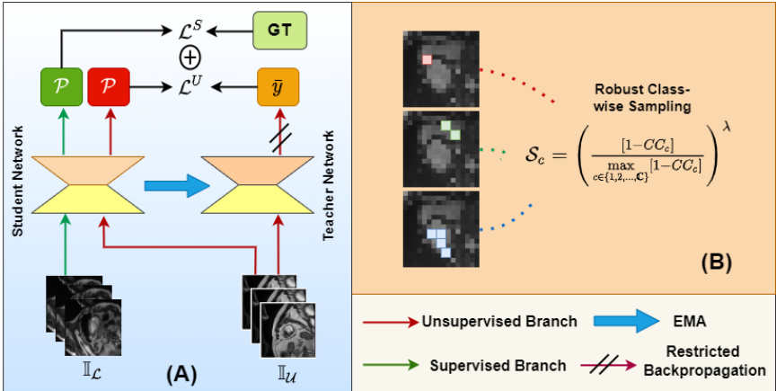
Fig. 1: Overall training strategy of the proposed method: (A) the basic studentteacher network, used as a backbone in our work, and (B) the Robust Class-wise Sampling that adaptively samples more pixels from the under-performing classes
图 1: 所提出方法的整体训练策略: (A) 基础学生-教师网络, 作为本工作的主干框架, (B) 鲁棒类别采样机制, 自适应地从表现欠佳的类别中采样更多像素
2.1 Basic Student-Teacher Framework
2.1 基础师生框架
Similar to [26], our network consists of a student-teacher framework, where the network learns through the student branch only, and the weights of the teacher model are updated by using an Exponential Moving Average (EMA). The student model is used to generate pseudo labels $\mathcal{V}$ on both labelled data $\mathbb{\mathrm{L}}{\mathcal{L}}$ with weak augmentations and unlabelled data $\mathbb{L}{\mathcal{U}}$ with strong augmentations. In contrast, the teacher model only generates pseudo labels on weakly augmented unlabelled data $\mathbb{L}_{\mathcal{U}}$ . The base student-teacher model is shown in Figure 1(A). The standard supervised and unsupervised loss functions ( $\mathcal{L}^{S}$ and $\mathcal{L^{\boldsymbol{U}}}$ ) can, therefore, be defined as:
与[26]类似,我们的网络采用师生框架(student-teacher framework),仅通过学生分支进行学习,教师模型的权重通过指数移动平均(EMA)更新。学生模型在弱增强的标注数据$\mathbb{\mathrm{L}}{\mathcal{L}}$和强增强的无标注数据$\mathbb{L}{\mathcal{U}}$上生成伪标签$\mathcal{V}$,而教师模型仅在弱增强的无标注数据$\mathbb{L}_{\mathcal{U}}$上生成伪标签。基础师生模型如图1(A)所示。标准监督损失函数$\mathcal{L}^{S}$和无监督损失函数$\mathcal{L^{\boldsymbol{U}}}$可定义为:
$$
\mathcal{L}^{S}=\frac{1}{\mathbb{N}{1}}\sum_{n=1}^{\mathbb{N}{1}}\frac{1}{h\times w}\sum_{i=1}^{h\times w}\mathcal{L}{C E}(\mathcal{P}{n,i},G T_{n,i})
$$
$$
\mathcal{L}^{S}=\frac{1}{\mathbb{N}{1}}\sum_{n=1}^{\mathbb{N}{1}}\frac{1}{h\times w}\sum_{i=1}^{h\times w}\mathcal{L}{C E}(\mathcal{P}{n,i},G T_{n,i})
$$
$$
\mathcal{L}^{U}=\frac{1}{\mathbb{N}{2}}\sum_{n=1}^{\mathbb{N}{2}}\frac{1}{h\times w}\sum_{i=1}^{h\times w}\mathcal{L}{C E}(\mathcal{P}{n,i},\bar{y}_{n,i})
$$
$$
\mathcal{L}^{U}=\frac{1}{\mathbb{N}{2}}\sum_{n=1}^{\mathbb{N}{2}}\frac{1}{h\times w}\sum_{i=1}^{h\times w}\mathcal{L}{C E}(\mathcal{P}{n,i},\bar{y}_{n,i})
$$
where, $h\times w$ is the image dimension, $\mathcal{L}{C E}$ represents the standard pixelwise cross-entropy loss, $\mathcal{P}{n,i}$ represents the prediction of $i^{t h}$ pixel of $n^{t h}$ image, $G T$ is the ground truth label, and $\bar{y}_{n,i}\in\bar{y}$ is the generated pseudo label for the corresponding pixel of the corresponding image.
其中,$h\times w$ 是图像尺寸,$\mathcal{L}{C E}$ 表示标准逐像素交叉熵损失,$\mathcal{P}{n,i}$ 表示第 $n$ 张图像第 $i$ 个像素的预测值,$G T$ 是真实标签,$\bar{y}_{n,i}\in\bar{y}$ 是对应图像对应像素生成的伪标签。
2.2 Dynamic Class-aware Learning
2.2 动态类感知学习
Formulation of Confidence Array Some of the methods in literature [20,14] address the imbalanced training in natural scene images by relying on classwise sample counts followed by ad-hoc weighting and sampling strategies. To this end, we propose maintaining three different performance indicators, namely
置信度数组的构建
文献[20,14]中的部分方法通过依赖类别样本计数并结合临时加权与采样策略,来解决自然场景图像中的训练不平衡问题。为此,我们提出维护三种不同的性能指标,即
Entropy, V ariance, and Confidence, in a class-wise confidence array to assess the performance of every class. We define Entropy indicator $\mathbb{E}_{c}$ for class $c$ as:
熵 (Entropy)、方差 (Variance) 和置信度 (Confidence) 组成类间置信度数组,用于评估每个类别的性能。我们将类别 $c$ 的熵指标 $\mathbb{E}_{c}$ 定义为:
$$
\mathbb{E}{c}=\frac{1}{\mathbb{N}{1}}\sum_{n=1}^{\mathbb{N}{1}}\frac{1}{\mathbb{N}{c}^{n}}\sum_{\substack{i=1}}^{\mathbb{N}{c}^{n}}\sum_{j=1}^{\mathbb{C}}\mathcal{P}{n,i}^{c}\log\mathcal{P}_{n,i}^{j};\forall c\in{1,2,3,...,\mathbb{C}}
$$
$$
\mathbb{E}{c}=\frac{1}{\mathbb{N}{1}}\sum_{n=1}^{\mathbb{N}{1}}\frac{1}{\mathbb{N}{c}^{n}}\sum_{\substack{i=1}}^{\mathbb{N}{c}^{n}}\sum_{j=1}^{\mathbb{C}}\mathcal{P}{n,i}^{c}\log\mathcal{P}_{n,i}^{j};\forall c\in{1,2,3,...,\mathbb{C}}
$$
where $\mathcal{P}{n,i}^{j}$ is the $j^{t h}$ channel prediction for the $i^{t h}$ pixel of $n^{t h}$ image. Similarly, we define V ariance and Confidence indicators $\mathbb{V}{c}$ and $\mathbb{C}o n_{c}$ respectively as:
其中 $\mathcal{P}{n,i}^{j}$ 表示第 $n$ 张图像第 $i$ 个像素的第 $j$ 个通道预测值。类似地,我们分别定义方差指标 $\mathbb{V}{c}$ 和置信度指标 $\mathbb{C}o n_{c}$ 为:
$$
\mathbb{V}{c}=\frac{1}{\mathbb{N}{1}}\sum_{n=1}^{\mathbb{N}{1}}\frac{1}{\mathbb{N}{c}^{n}}\sum_{i=1}^{\mathbb{N}{c}^{n}}\left(\operatorname*{max}{j\in{1,2,..,\mathbb{C}}}[\mathcal{P}{n,i}^{j}]-\mathcal{P}_{n,i}^{c}\right);\forall c\in{1,2,3,...,\mathbb{C}}
$$
$$
\mathbb{V}{c}=\frac{1}{\mathbb{N}{1}}\sum_{n=1}^{\mathbb{N}{1}}\frac{1}{\mathbb{N}{c}^{n}}\sum_{i=1}^{\mathbb{N}{c}^{n}}\left(\operatorname*{max}{j\in{1,2,..,\mathbb{C}}}[\mathcal{P}{n,i}^{j}]-\mathcal{P}_{n,i}^{c}\right);\forall c\in{1,2,3,...,\mathbb{C}}
$$
$$
\mathbb{C}o n_{c}=\frac{1}{\mathbb{N}{1}}\sum_{n=1}^{\mathbb{N}{1}}\frac{1}{\mathbb{N}{c}^{n}}\sum_{i=1}^{\mathbb{N}{c}^{n}}\mathcal{P}_{n,i}^{c}~;~\forall c\in{1,2,3,...,\mathbb{C}}
$$
$$
\mathbb{C}o n_{c}=\frac{1}{\mathbb{N}{1}}\sum_{n=1}^{\mathbb{N}{1}}\frac{1}{\mathbb{N}{c}^{n}}\sum_{i=1}^{\mathbb{N}{c}^{n}}\mathcal{P}_{n,i}^{c}~;~\forall c\in{1,2,3,...,\mathbb{C}}
$$
Fuzzy Confidence Fusion We combine the three class-wise performance indicators $\mathbb{E}{c}$ , $\mathbb{V}{c}$ , and $\mathbb{C}o n_{c}$ to generate the final $C C$ score using a fuzzy fusion scheme. Gompertz function was experimentally adopted for fuzzy fusion as explained in the supplementary material. First, we generate a class-wise fuzzy rank of different performance indicators using a re-parameterized Gompertz function [18] as:
模糊置信度融合
我们将三个类别性能指标 $\mathbb{E}{c}$、$\mathbb{V}{c}$ 和 $\mathbb{C}o n_{c}$ 通过模糊融合方案结合,生成最终的 $C C$ 分数。如补充材料所述,实验采用 Gompertz 函数进行模糊融合。首先,我们使用重新参数化的 Gompertz 函数 [18] 生成不同性能指标的类别模糊排序:
$$
\mathbb{R}{c}^{k}=1-e^{-e^{-2\cdot n o r m(x_{c}^{k})}},\mathrm{ where~}x_{c}^{k}\in{\mathbb{E}{c},\mathbb{V}{c},\mathbb{C}o n_{c}},
$$
$$
\mathbb{R}{c}^{k}=1-e^{-e^{-2\cdot n o r m(x_{c}^{k})}},\mathrm{ 其中~}x_{c}^{k}\in{\mathbb{E}{c},\mathbb{V}{c},\mathbb{C}o n_{c}},
$$
where, $n o r m()$ signifies normalization function, $\mathbb{R}{c}^{k}$ is in range [0.127, 0.632], where a higher confidence score gives better (lower) rank. The selection of the objective fuzzy function is based on model performance. For detailed analysis, please refer to the supplementary file. Now, if $M^{k}$ represents top $m$ ranks for class $c$ , then we compute a complement of confidence factor sum $(C C F_{c})$ and fuzzy rank sum $(F R_{c})$
其中,$norm()$ 表示归一化函数,$\mathbb{R}{c}^{k}$ 的范围在 [0.127, 0.632] 之间,置信度分数越高,排名越好(越低)。目标模糊函数的选择基于模型性能。详细分析请参阅补充文件。现在,如果 $M^{k}$ 表示类别 $c$ 的前 $m$ 个排名,那么我们计算置信因子补集和 $(CCF_{c})$ 以及模糊排名和 $(FR_{c})$
where, $P_{c}^{C C F}$ and $P_{c}^{F R}$ are the penalty values (set to 0 and 0.632 respectively) for class $c$ to suppress the unlikely winner. The final cumulative confidence $(C C)$ score is thereafter computed as:
其中,$P_{c}^{C C F}$ 和 $P_{c}^{F R}$ 是类别 $c$ 的惩罚值(分别设为 0 和 0.632),用于抑制不太可能的胜出者。最终累积置信度 $(C C)$ 分数随后计算为:
$$
C C_{c}=C C F_{c}\times F R_{c}\forall c\in{1,2,...\mathbb{C}}
$$
$$
C C_{c}=C C F_{c}\times F R_{c}\forall c\in{1,2,...\mathbb{C}}
$$
The obtained $C C$ score is updated after $t^{\mathrm{th}}$ training iteration as:
在第 $t^{\mathrm{th}}$ 次训练迭代后,获得的 $C C$ 分数更新如下:
$$
C C_{c}^{t}\longleftarrow\alpha C C_{c}^{t-1}+(1-\alpha)C C_{c}^{t};\forall c\in{1,2,3,...,\mathbb{C}}
$$
$$
C C_{c}^{t}\longleftarrow\alpha C C_{c}^{t-1}+(1-\alpha)C C_{c}^{t};\forall c\in{1,2,3,...,\mathbb{C}}
$$
where, $\alpha$ is the momentum parameter, set to 0.999 experimentally.
其中,$\alpha$ 是动量参数,实验设定为 0.999。
Robust Class-wise Sampling We obtain the category-wise confidence score and identify the under-performing classes as described in section 2.2. To alleviate the problem of class-wise training bias, i.e., preventing well-performing classes from overwhelming model training and anchoring the training on a sparse set of under-performing classes, we propose a class-wise sampling rate $S_{c}$ as:
稳健的类别抽样策略
我们按照2.2节所述方法获取各类别的置信度分数,并识别表现欠佳的类别。为缓解类别训练偏差问题(即防止表现优异的类别主导模型训练,同时避免训练过度集中于少量欠佳类别),我们提出以下类别抽样率$S_{c}$公式:
$$
\mathcal{S}{c}=\left(\frac{[1-C C_{c}]}{\underset{c\in{1,2,\ldots,\mathbb{C}}}{\operatorname*{max}}[1-C C_{c}]}\right)^{\lambda}
$$
$$
\mathcal{S}{c}=\left(\frac{[1-C C_{c}]}{\underset{c\in{1,2,\ldots,\mathbb{C}}}{\operatorname*{max}}[1-C C_{c}]}\right)^{\lambda}
$$
where $\lambda$ is a tunable parameter. Instead of sampling all the available pixels for the unsupervised loss formulation, we sample random pixels from class $c$ with sampling rate of $S_{c}$ . So $\mathcal{L^{\boldsymbol{U}}}$ in Equation 2 can be reformulated as:
其中 $\lambda$ 是一个可调参数。我们并非对所有可用像素进行无监督损失计算,而是以 $S_{c}$ 的采样率从类别 $c$ 中随机选取像素。因此,公式2中的 $\mathcal{L^{\boldsymbol{U}}}$ 可改写为:
$$
\mathcal{L}^{U}=\frac{1}{\mathrm{N}{2}}\sum_{n=1}^{\mathrm{N}{2}}\frac{1}{\left(\displaystyle\sum_{i=1}^{h\times w}\mathbb{1}{n,i}\right)}\sum_{i=1}^{h\times w}\mathbb{1}{n,i}\mathcal{L}{C E}(\mathcal{P}{n,i},\bar{y}_{n,i})
$$
$$
\mathcal{L}^{U}=\frac{1}{\mathrm{N}{2}}\sum_{n=1}^{\mathrm{N}{2}}\frac{1}{\left(\displaystyle\sum_{i=1}^{h\times w}\mathbb{1}{n,i}\right)}\sum_{i=1}^{h\times w}\mathbb{1}{n,i}\mathcal{L}{C E}(\mathcal{P}{n,i},\bar{y}_{n,i})
$$
where $\mathbb{1}$ is the binary value operator. The value ${\mathbb{1}}{n,i}=0$ if the $i^{t h}$ pixel from the $n^{t h}$ image is not sampled according to sampling rate $S_{c}$ , otherwise set to $^{1}$ . Figure $\mathrm{1(B)}$ represents the proposed class-wise sampling strategy.
其中 $\mathbb{1}$ 是二值运算符。当第 $n$ 张图像的第 $i^{t h}$ 像素未根据采样率 $S_{c}$ 被采样时,${\mathbb{1}}_{n,i}=0$,否则设为 $^{1}$。图 1(B) 展示了提出的按类别采样策略。
Dynamic Training Stabilization As the model performance strictly relies upon the quality of pseudo labels, the under-performing categories insert a significant amount of noise in the pseudo label, hindering the training process. Methods in literature [17] set a higher threshold value to remove the underperforming classes, although this firm criterion leads to lower recall value for those categories, affecting the overall training. We utilize a dynamic modulation of weights to alleviate this problem for better training stabilization. This aims to redistribute the loss contribution from convincing and under-performing samples, i.e., more weights to the convincing classes. The unsupervised loss in Equation 11 can be reformulated as:
动态训练稳定化
由于模型性能严格依赖于伪标签的质量,表现不佳的类别会在伪标签中引入大量噪声,阻碍训练过程。文献[17]中的方法通过设置更高阈值来剔除表现不佳的类别,但这一严格标准会导致这些类别的召回率降低,影响整体训练效果。我们采用动态权重调制来缓解该问题,从而实现更稳定的训练。该方法旨在重新分配可信样本与欠佳样本对损失的贡献度(即给予可信类别更高权重)。公式11中的无监督损失可改写为:
$$
\mathcal{L}^{U}=\frac{1}{\mathrm{N}{2}}\sum_{n=1}^{\mathrm{N}{2}}\frac{1}{\left(\displaystyle\sum_{i=1}^{h\times w}\mathcal{W}{n,i}\right)}\sum_{i=1}^{h\times w}\mathcal{W}{n,i}\mathcal{L}{C E}(\mathcal{P}{n,i},\bar{y}_{n,i})
$$
$$
\mathcal{L}^{U}=\frac{1}{\mathrm{N}{2}}\sum_{n=1}^{\mathrm{N}{2}}\frac{1}{\left(\displaystyle\sum_{i=1}^{h\times w}\mathcal{W}{n,i}\right)}\sum_{i=1}^{h\times w}\mathcal{W}{n,i}\mathcal{L}{C E}(\mathcal{P}{n,i},\bar{y}_{n,i})
$$
where $\mathcal{W}_{n,i}$ is the weight provided for the $i^{t h}$ pixel in $n^{t h}$ image in the final unsupervised loss formulation, and can be defined as:
其中 $\mathcal{W}_{n,i}$ 是第 $n$ 张图像中第 $i^{t h}$ 个像素在最终无监督损失公式中的权重,可定义为:
$$
\mathcal{W}{n,i}=\mathbb{1}{n,i}\operatorname*{max}{c\in{1,2,...,\mathbb{C}}}[\mathcal{P}_{n,i}]^{\beta}
$$
$$
\mathcal{W}{n,i}=\mathbb{1}{n,i}\operatorname*{max}{c\in{1,2,...,\mathbb{C}}}[\mathcal{P}_{n,i}]^{\beta}
$$
where $\beta$ is a tunable parameter. The final loss function is computed as:
其中 $\beta$ 是一个可调参数。最终损失函数计算为:
$$
\mathcal{L}_{t o t a l}=\mathcal{L}^{U}+\zeta\mathcal{L}^{S},
$$
$$
\mathcal{L}_{t o t a l}=\mathcal{L}^{U}+\zeta\mathcal{L}^{S},
$$
where $\zeta$ is a tunable parameter. The value of $\zeta$ decreases with an increase in the number of iterations, limiting the contribution of supervised loss term $\mathcal{L}^{S}$ in the overall loss in the later stage of training.
其中 $\zeta$ 是一个可调参数。$\zeta$ 的值随着迭代次数的增加而减小,从而限制了监督损失项 $\mathcal{L}^{S}$ 在训练后期整体损失中的贡献。
3 Experiments and Results
3 实验与结果
3.1 Dataset and Implementation Details
3.1 数据集与实现细节
The model is evaluated on two publicly available cardiac MRI datasets. (1) the ACDC dataset [9], hosted in MICCAI17, contains 100 patients’ cardiac MR volumes, where for every patient it has around 15 volumes covering the entire cardiac cycle, and expert annotations for left and right ventricles and myocardium. (2) The MMWHS dataset [31] consists of 20 cardiac MRI samples with expert annotations for seven structures: left and right ventricles, left and right atrium, pulmonary artery, myocardium, and aorta. The datasets are distributed into a $4:1$ ratio of training and validation sets for both cases. To validate the model performance on different label percentages, we use $1.25%$ , $2.5%$ , and $10%$ labelled data from ACDC and $10%$ , $20%$ , and 40% labelled data from MMWHS for training purposes (label percentage is taken in accordance to other methods in literature). The values of $\beta$ in Equation 13 and $\lambda$ in Equation 10 are taken as 1.5 and 2.5, respectively (experimental analysis in supplementary file). The experi ment ation is implemented using Tesla K80 GPU with 16GB RAM. An SGD optimizer with an initial learning rate $1e{-4}$ , momentum of 0.9, and weight decay of 0.0001 was employed. Three widely used metrics are used for the evaluation purpose: Dice Similarity Score (DSC), Average Symmetric Distance (ASD), and Hausdorff Distance (HD) [2].
该模型在两个公开可用的心脏MRI数据集上进行评估。(1) MICCAI17主办的ACDC数据集[9]包含100名患者的心脏MR体积数据,每位患者约有15个覆盖整个心动周期的体积数据,以及专家标注的左右心室和心肌。(2) MMWHS数据集[31]包含20个心脏MRI样本,专家标注了七个结构:左右心室、左右心房、肺动脉、心肌和主动脉。两个数据集的训练集与验证集均按4:1比例划分。为验证模型在不同标注比例下的性能,我们使用ACDC数据集的1.25%、2.5%和10%标注数据,以及MMWHS数据集的10%、20%和40%标注数据进行训练(标注比例参照文献中其他方法设定)。公式13中的β值和公式10中的λ值分别取1.5和2.5(实验分析见补充文件)。实验采用配备16GB内存的Tesla K80 GPU实现,使用初始学习率为1e-4、动量为0.9、权重衰减为0.0001的SGD优化器。评估采用三个常用指标:Dice相似系数(DSC)、平均对称距离(ASD)和豪斯多夫距离(HD)[2]。
3.2 Quantitative Performance Evaluation
3.2 定量性能评估
To empirically illustrate the effective segmentation ability of the proposed model in a semi-supervised environment, we evaluate our proposed method on the ACDC and MMWHS datasets by training the model using different percentages of labelled data (see Figure 2). For the ACDC dataset, the reported DSC, ASD and HD values are 0.746, 0.677, 2.409, respectively while using 1.25% training samples, 0.842, 0.614, 2.009 corresponding to $2.5%$ training labels, 0.889, 0.511, 1.804 for $10%$ and 0.902, 0.489, 1.799 while using $100%$ samples for training. We consider the $100%$ training labels utilization as a fully supervised functioning for comparative analysis. As can be inferred from Figure 2A, the segmentation performance of the proposed model utilizing only a handful of labels is comparable to the fully supervised counterpart. A similar trend is also observed in Figure 2B, where the DSC score while using $10%$ , 20%, 40% and $100%$ training samples are 0.626, 0.791, 0.815 and 0.826 respectively. The reported ASD scores for the respective cases are 2.397, 1.798, 1.355 and 1.317, respectively. The HD score for the 10% case is 5.001, which is slightly higher, but while using 40% of the labels for training, the HD score drops down to 2.221, comparable to the fully supervised case with an HD of 2.183.
为实证验证所提模型在半监督环境下的有效分割能力,我们在ACDC和MMWHS数据集上评估了该方法,通过使用不同比例的标注数据训练模型(见图2)。对于ACDC数据集,当使用1.25%训练样本时,报告的DSC、ASD和HD值分别为0.746、0.677、2.409;使用2.5%标注数据时对应为0.842、0.614、2.009;使用10%时为0.889、0.511、1.804;而使用100%样本训练时达到0.902、0.489、1.799。我们将100%标注数据的使用视为全监督基准进行对比分析。从图2A可推断,仅用少量标注时,所提模型的分割性能已接近全监督水平。图2B也呈现相似趋势:当使用10%、20%、40%和100%训练样本时,DSC分数分别为0.626、0.791、0.815和0.826。各情况下报告的ASD分数依次为2.397、1.798、1.355和1.317。10%数据时的HD分数为5.001略高,但使用40%标注训练时HD降至2.221,与全监督情况下的2.183相当。
3.3 Comparison with State-of-the-art
3.3 与最先进技术的对比
To prove the effectiveness of the proposed model, we have performed its comparative analysis with some state-of-the-art models [13,15,12,11] which is shown in Table 1. As can be inferred, for the ACDC dataset, the average DSC score as reported by our model while using $1.25%$ and $2.5%$ training samples is the second best with the state-of-the-art performance given by Global $^+$ Local CL [10], and PCL [30] respectively. For $10%$ training samples, on the other hand, the state-of-the-art performance is reported by the proposed model (DSC=0.889). For the MMWHS dataset, the proposed model surpasses all the existing models in terms of the average DSC score while using $10%$ , 20% or 40% of the training samples, with an average 5% margin over the second-best performing model. Another important observation is that methods like [30,1,15] fail to produce satisfactory results using very few annotations (1.25% and $10%$ labelled data for ACDC and MMWHS, respectively). In contrast, our proposed method performs quite consistently as compared to those. We record class-wise DSC and sensitivity to observe the improvements for under-performing classes. Observed DSC and sensitivity are (0.934, 0.883, 0.877) and (0.964, 0.925, 0.911) for classes LV, RV, and MYO respectively using $10%$ labelled data of ACDC. Our method achieves an improvement of $\approx2-5%$ for under-performing classes (RV, MYO) than the baseline and literature. Similar improvements are observed across the classes in other experimental settings, both for ACDC and MMWHS.
为验证所提模型的有效性,我们将其与现有先进模型[13,15,12,11]进行了对比分析,结果如 表 1 所示。可以看出,在ACDC数据集上,当使用$1.25%$和$2.5%$训练样本时,我们模型报告的平均DSC分数仅次于当前最优的Global$^+$Local CL[10]和PCL[30]方法。而在使用$10%$训练样本时,所提模型取得了最佳性能(DSC=0.889)。对于MMWHS数据集,在使用$10%$、20%或40%训练样本时,所提模型在平均DSC分数上均超越现有所有模型,较第二名保持约5%的优势。值得注意的是,[30,1,15]等方法在极少量标注数据下(ACDC的1.25%和MMWHS的$10%$)表现欠佳,而我们的方法则保持稳定性能。通过记录各类别的DSC和灵敏度,我们发现使用ACDC数据集$10%$标注数据时,LV、RV和MYO类别的DSC分别为(0.934, 0.883, 0.877),灵敏度为(0.964, 0.925, 0.911)。对于表现较弱的RV和MYO类别,我们的方法较基线模型和文献结果实现了约$\approx2-5%$的提升。在ACDC和MMWHS的其他实验设置中,各类别均观察到类似的改进趋势。

Fig. 2: Quantitative segmentation performance of our proposed method using different percentage of labelled data of ACDC and MMWHS.
图 2: 使用不同比例标注数据的ACDC和MMWHS数据集上我们提出方法的定量分割性能。
Table 1: Comparison of the proposed method with state-of-the-art frameworks on ACDC and MMWHS datasets.
表 1: 所提方法与ACDC和MMWHS数据集上先进框架的对比。
| 方法 | Average DsC (ACDC) | AverageDsC (MMWHS) | ||||
|---|---|---|---|---|---|---|
| L=1.25% | L=2.5% | L=10% | L=10% | L=20% | L=40% | |
| Global CL[13] | 0.729 | - | 0.847 | 0.5 | 0.659 | 0.785 |
| PCL [30] | 0.671 | 0.85 | 0.885 | - | - | |
| ContextRestoration [12] | 0.625 | 0.714 | 0.851 | 0.482 | 0.654 | 0.783 |
| Label Efficient [15] | 二 | 二 | 二 | 0.382 | 0.553 | 0.764 |
| Data Aug [11] | 0.731 | 0.786 | 0.865 | 0.529 | 0.661 | 0.785 |
| Self Train [1] | 0.69 | 0.749 | 0.86 | 0.563 | 0.691 | 0.801 |
| Global + Local CL [10] | 0.757 | 0.826 | 0.886 | 0.617 | 0.710 | 0.794 |
| Ours | 0.746 | 0.842 | 0.889 | 0.626 | 0.791 | 0.815 |
Table 2: Ablation study to identify the effectiveness of Robust Class-wise Sampling (RCS), Dynamic Training Stabilization (DTS), Fuzzy Fusion on ACDC and MMWHS datasets using $10%$ and $40%$ labelled data respectively.
表 2: 在分别使用$10%$和$40%$标注数据的ACDC和MMWHS数据集上,验证鲁棒类采样(RCS)、动态训练稳定(DTS)和模糊融合效果的消融实验。
| 学生-教师模型 (基础模型) | RCS | DTS | ACDC | MMWHS |
|---|---|---|---|---|
| 简单平均规则融合 | 模糊 | DSC | ||
| 0.817 | ||||
| √ | 0.855 | |||
| 人 | 人 | 0.861 | ||
| 人 | 人 | √ | 0.872 | |
| 人 | √ | √ | 0.889 |
3.4 Ablation Studies
3.4 消融实验
To find out the potency of different components used in the formulation of our proposed scheme, we perform a detailed ablation study, as shown in Table 2. We use a student-teacher framework as the baseline for all the ablation experiments, which produces an average DSC of 0.819 and 0.734 upon evaluation on ACDC and MMWHS datasets, respectively, as a standalone model. Then, we perform two sets of experiments to identify the importance of Robust Class-wise Sampling (RCS) and fuzzy fusion. Instead of fuzzy fusion, as described in Equation 8, first we form the CC score by just simple averaging the three performance indicators: $C C_{c}=(\mathbb{E}{c}+\mathbb{V}{c}+\mathbb{C}o n_{c})/3$ . This, along with the RCS, improves the baseline performance by $4.65%$ and $6.40%$ in terms of DSC on ACDc and MMWHS, respectively. To fully utilize the potential of RCS, when we evaluate it along with fuzzy fusion, the model outperforms the baseline DSC by a margin of $6.73%$ and $7.91%$ respectively on the two datasets. The fuzzy fusion scheme adaptively prioritizes the confidence scores for individual samples rather than using any preset fixed weights to combine the confidence scores. On the other hand, Dynamic Training Stabilization (DTS) and RCS alleviate the problem of class-wise biased training by adaptively prioritizing the under-performing sample classes. This is also justified by the improvements of $\approx2%$ and $\approx3%$ on ACDC and MMWHS brought by DTS when used on top of RCS with a simple average rule. Furthermore, we present our proposed scheme using DTS and a fuzzy fusion scheme in RCS to achieve the best DSC of 0.889 and 0.815 on ACDC and MMWHS, respectively. Additionally, we also observe the variation of model performance by using three confidence indicators individually (refer to supplementary file).
为了验证所提方案中各组件的有效性,我们进行了详细的消融实验,结果如表 2 所示。以师生框架作为所有消融实验的基线模型,其单独在ACDC和MMWHS数据集上的平均DSC分别为0.819和0.734。随后我们通过两组实验验证鲁棒类级采样(RCS)和模糊融合的重要性:首先不使用公式8的模糊融合方法,而是通过简单平均三个性能指标构建CC分数$C C_{c}=(\mathbb{E}{c}+\mathbb{V}{c}+\mathbb{C}o n_{c})/3$。该方法与RCS结合后,在ACDC和MMWHS数据集上的DSC分别比基线提升4.65%和6.40%。当RCS与模糊融合协同工作时,模型在两个数据集上的DSC相较基线分别提升6.73%和7.91%。模糊融合机制通过自适应调整各样本的置信度权重,取代了预设固定权重的融合方式;而动态训练稳定器(DTS)与RCS则通过自适应关注表现欠佳的样本类别,缓解了类级训练偏差问题。当在RCS基础上应用简单平均规则的DTS时,ACDC和MMWHS数据集的性能分别提升约2%和约3%。最终,我们提出的结合DTS与模糊融合的RCS方案,在ACDC和MMWHS数据集上分别达到0.889和0.815的最佳DSC值。此外,我们还单独测试了三个置信度指标对模型性能的影响(详见补充材料)。
4 Conclusion
4 结论
The scarcity of pixel-level annotations has always been a significant hurdle for medical image segmentation. Besides, a limitation of the deep-learning-based strategies is that they get biased toward the majority class, thereby affecting the overall model performance. To this end, our work addresses both issues by forming a class-wise performance-aware dynamic learning strategy. Experimentation on two publicly available cardiac MRI datasets exhibits the superiority of the proposed method over the state-of-the-art methods. In future, we plan to extend the work by designing it as a fine-tuning strategy on top of a contrastive pre-training for more effective utilization of the global context.
像素级标注的稀缺性一直是医学图像分割领域的重大障碍。此外,基于深度学习的策略存在偏向多数类别的局限性,从而影响模型整体性能。为此,我们通过构建一种类别性能感知的动态学习策略来解决这两个问题。在两个公开的心脏MRI数据集上的实验表明,该方法优于当前最先进的技术。未来,我们计划将该方法扩展为对比预训练基础上的微调策略,以更有效地利用全局上下文信息。
References
参考文献
Supplementary Material: Addressing Class Imbalance in Semi-supervised Image Segmentation: A Study on Cardiac MRI
补充材料:解决半监督图像分割中的类别不平衡问题:心脏MRI研究
Hritam Basak $^1$ ⋆, Sagnik Ghosal $^{1}$ , and Ram Sarkar $^2$
Hritam Basak $^1$ ⋆, Sagnik Ghosal $^{1}$, 和 Ram Sarkar $^2$
1 Dept. of Electrical Engineering, Jadavpur University, Kolkata, India 2 Dept. of Computer Science and Engineering, Jadavpur University, Kolkata, India {hr it amba sak 48, s agni kg hos al 1999, ramjucse}@gmail.com
1 印度加尔各答贾达普大学电气工程系
2 印度加尔各答贾达普大学计算机科学与工程系
{hr it amba sak 48, s agni kg hos al 1999, ramjucse}@gmail.com
Table 1: Variation of DSC w.r.t. $\beta$ in DTS
表 1: DTS中DSC随$\beta$的变化
| B | ACDC | MMWHS (10%标注) (40%标注) |
|---|---|---|
| 0.0 | 0.876 | 0.807 |
| 0.5 | 0.882 | 0.810 |
| 1.0 | 0.887 | 0.812 |
| 1.5 | 0.889 | 0.815 |
| 2.0 | 0.881 | 0.813 |
| 2.5 | 0.879 | 0.808 |
| 3.0 | 0.878 | 0.806 |
Table 2: Variation of DSC w.r.t. $\lambda$ in RCS
表 2: RCS中DSC随$\lambda$的变化
| λ | ACDC | MMWHS (10%标注)(40%标注) |
|---|---|---|
| 1.0 | 0.879 | 0.805 |
| 1.5 | 0.881 | 0.808 |
| 2.0 | 0.886 | 0.811 |
| 2.5 | 0.889 | 0.815 |
| 3.0 | 0.887 | 0.811 |
| 3.5 | 0.886 | 0.811 |
| 4.0 | 0.884 | 0.810 |
Table 3: Performance for different confidence indicators on Robust Class-wise Sampling using $10%$ and $40%$ labelled data for ACDC and MMWHS respectively
表 3: 在ACDC和MMWHS数据集上分别使用 $10%$ 和 $40%$ 标注数据时,不同置信度指标在鲁棒类采样中的性能表现
| PerformanceIndicator | DTS | ACDC | MMWHS | ||||
|---|---|---|---|---|---|---|---|
| DSC | ASD | HD | DSC | ASD | HD | ||
| Entropy (E) | 0.847 | 1.836 | 0.539 | 0.788 | 2.246 | 1.474 | |
| √ | 0.866 | 1.821 | 0.529 | 0.793 | 2.234 | 1.368 | |
| Variance (V) | 0.855 | 1.837 | 0.540 | 0.776 | 2.244 | 1.477 | |
| 0.864 | 1.826 | 0.531 | 0.787 | 2.237 | 1.372 | ||
| Confidence (Con) | 0.866 | 1.825 | 0.527 | 0.784 | 2.327 | 1.441 | |
| √ | 0.878 | 1.811 | 0.519 | 0.809 | 2.228 | 1.361 | |
| Cumulative Confidence (CC) | 0.879 | 1.809 | 0.516 | 0.810 | 2.230 | 1.362 | |
| 0.889 | 1.804 | 0.511 | 0.815 | 2.221 | 1.355 |
References
参考文献
- Bai, Wenjia, et al. "Semi-supervised learning for network-based cardiac MR image segmentation." International Conference on Medical Image Computing and Computer-Assisted Intervention. Springer, Cham, 2017.
- Bai, Wenjia, 等. "基于网络的半监督学习用于心脏磁共振图像分割." 国际医学图像计算与计算机辅助干预会议. Springer, Cham, 2017.
Table 4: Variation of model performance on ACDC and MMWHS datasets while using different fuzzy functions in Robust Class-wise Sampling
表 4: 在Robust Class-wise Sampling中使用不同模糊函数时模型在ACDC和MMWHS数据集上的性能变化
| Fuzzy F Function | Average DsC (ACDC) | Average DSC (MMWHS) | ||||
|---|---|---|---|---|---|---|
| L=1.25% | L=2.5% | L=10% | L=10% | L=20% | L=40% | |
| Mitscherlich [4] | 0.737 | 0.834 | 0.881 | 0.612 | 0.785 | 0.798 |
| Blumberg [2] | 0.740 | 0.839 | 0.886 | 0.618 | 0.789 | 0.812 |
| Weibull 5 | 0.739 | 0.837 | 0.885 | 0.618 | 0.788 | 0.813 |
| Gompertz | 0.746 | 0.842 | 0.889 | 0.626 | 0.791 | 0.815 |

Fig. 1: Visual comparison of our proposed method with the available ground truth (GT), along with several other state-of-the-art methods: PCL [6], Self Train [1], and Global $^+$ Local CL [3]
图 1: 我们提出的方法与现有真实数据 (GT) 的视觉对比,以及其他几种先进方法:PCL [6]、Self Train [1] 和 Global $^+$ Local CL [3]