nnFormer: Volumetric Medical Image Segmentation via a 3D Transformer
nnFormer: 基于3D Transformer的医学图像体积分割
Abstract— Transformer, the model of choice for natural language processing, has drawn scant attention from the medical imaging community. Given the ability to exploit long-term dependencies, transformers are promising to help atypical convolutional neural networks to overcome their inherent shortcomings of spatial inductive bias. However, most of recently proposed transformer-based segmentation approaches simply treated transformers as assisted modules to help encode global context into convolutional representations. To address this issue, we introduce nnFormer (i.e., not-another transFormer), a 3D transformer for volumetric medical image segmentation. nnFormer not only exploits the combination of interleaved convolution and self-attention operations, but also introduces local and global volume-based self-attention mechanism to learn volume representations. Moreover, nnFormer proposes to use skip attention to replace the traditional concatenation/summation operations in skip connections in U-Net like architecture. Experiments show that nnFormer significantly outperforms previous transformer-based counterparts by large margins on three public datasets. Compared to nnUNet, nnFormer produces significantly lower HD95 and comparable DSC results. Furthermore, we show that nnFormer and nnUNet are highly complementary to each other in model ensembling. Codes and models of nnFormer are available at https://git.io/JSf3i.
摘要— Transformer作为自然语言处理的首选模型,在医学影像领域却鲜有关注。鉴于其捕捉长程依赖关系的能力,Transformer有望帮助非典型卷积神经网络克服其固有的空间归纳偏置缺陷。然而,近期多数基于Transformer的分割方法仅将其作为辅助模块,用于将全局上下文编码到卷积表示中。为此,我们提出了nnFormer(即"非另一种Transformer"),这是一种用于三维医学图像分割的Transformer架构。nnFormer不仅融合了交错卷积与自注意力操作,还引入了基于局部和全局体素的自注意力机制来学习体积表征。此外,nnFormer创新性地采用跳跃注意力机制,取代了类似U-Net架构中跳跃连接传统的拼接/求和操作。实验表明,在三个公开数据集上,nnFormer以显著优势超越了此前基于Transformer的方法。与nnUNet相比,nnFormer在HD95指标上显著更优,DSC结果则相当。我们进一步证明,nnFormer与nnUNet在模型集成中具有高度互补性。nnFormer的代码与模型已开源:https://git.io/JSf3i。
Index Terms— Transformer, Attention Mechanism, Volumetric Image Segmentation
关键词— Transformer, 注意力机制 (Attention Mechanism), 体积图像分割 (Volumetric Image Segmentation)
I. INTRODUCTION
I. 引言
Transformer [1], which has become the de-facto choice for natural language processing (NLP) problems, has recently been widely exploited in vision-based applications [2]–[5]. The core idea behind is to apply the self-attention mechanism (Corresponding author: Liansheng Wang and Yizhou Yu.)
Transformer [1] 已成为自然语言处理 (NLP) 问题的实际选择,最近在视觉应用中得到了广泛利用 [2]–[5]。其核心思想是应用自注意力机制 (通讯作者: Liansheng Wang 和 Yizhou Yu)。
This work was done when Hong-Yu Zhou was a visiting student at Xiamen University.
本工作完成于周鸿宇在厦门大学访学期间。
Hong-Yu Zhou, Jiansen Guo, Yinghao Zhang and Liansheng Wang are with the Department of Computer Science, Xiamen University, Siming District, Xiamen, Fujian Province, P.R. China (email: w hu zhou hong yu@gmail.com, jsguo@stu.xmu.edu.cn, zhangyinghao@stu.xmu.edu.cn, lswang@xmu.edu.cn).
周鸿宇、郭建森、张英豪和王连生均就职于中华人民共和国福建省厦门市思明区厦门大学计算机科学系 (邮箱: w hu zhou hong yu@gmail.com, jsguo@stu.xmu.edu.cn, zhangyinghao@stu.xmu.edu.cn, lswang@xmu.edu.cn)。
Hong-Yu Zhou and Yizhou Yu are with the Department of Computer Science, The University of Hong Kong, Pokfulam, Hong Kong (e-mail: yizhouy@acm.org).
周鸿宇和Yizhou Yu就职于香港大学计算机科学系,香港薄扶林 (e-mail: yizhouy@acm.org)。
Xiaoguang Han is with the Shenzhen Research Institute of Big Data, The Chinese University of Hong Kong (Shenzhen), Shenzhen, Guangdong Province, P.R. China (email: han xiao guang@cuhk.edu.cn).
Xiaoguang Han就职于香港中文大学(深圳)大数据研究院,中国广东省深圳市 (邮箱: han xiao guang@cuhk.edu.cn)。
Lequan Yu is with the Department of Statistics and Actuarial Science, The University of Hong Kong, Pokfulam, Hong Kong (e-mail: lqyu@hku.hk).
Lequan Yu就职于香港大学统计与精算学系,香港薄扶林 (邮箱: lqyu@hku.hk)。
First two authors contributed equally.
前两位作者贡献均等。
to capture long-range dependencies. Compared to convolutional neural networks (i.e., convnets [6]), transformer relaxes the inductive bias of locality, making it more capable of dealing with non-local interactions [7]–[9]. It has also been investigated that the prediction errors of transformers are more consistent with those of humans than convnets [10].
捕捉长距离依赖关系。与卷积神经网络 (即convnets [6]) 相比,Transformer 放宽了局部性的归纳偏置,使其更擅长处理非局部交互 [7]–[9]。研究还发现,Transformer 的预测误差比卷积网络更符合人类误差模式 [10]。
Given the fact that transformers are naturally more advantageous than convnets, there are a number of approaches trying to apply transformers to the field of medical image analysis. Chen et al. [11] first time proposed TransUNet to explore the potential of transformers in the context of medical image segmentation. The overall architecture of TransUNet is similar to that of U-Net [12], where convnets act as feature extractors and transformers help encode the global context. In fact, one major characteristic of TransUNet and most of its followers [13]–[16] is to treat convnets as main bodies, on top of which transformers are further applied to capture long-term dependencies. However, such feature may cause a problem, which is the advantages of transformers are not fully exploited. In other words, we believe one- or two-layer transformers are not enough to entangle long-term dependencies with convolutional representations that often contain precise spatial information and provide hierarchical concepts.
鉴于Transformer天然比卷积网络更具优势,已有多种方法尝试将Transformer应用于医学图像分析领域。Chen等人[11]首次提出TransUNet来探索Transformer在医学图像分割中的潜力。TransUNet的整体架构与U-Net[12]类似,其中卷积网络作为特征提取器,而Transformer则帮助编码全局上下文。实际上,TransUNet及其大多数后续研究[13]-[16]的一个主要特点是将卷积网络作为主体,在此基础上进一步应用Transformer来捕获长程依赖关系。然而,这种特性可能导致一个问题,即Transformer的优势未能得到充分发挥。换句话说,我们认为仅使用一两层Transformer不足以将长程依赖关系与卷积表示充分融合,后者通常包含精确的空间信息并提供层次化概念。
To address the above issue, some researchers [17]–[19] started to use transformers as the main stem in segmentation models. Karimi et al. [17] first time introduced a convolution-free segmentation model by forwarding flattened image representations to transformers, whose outputs are then reorganized into 3D tensors to align with segmentation masks. Recently, Swin Transformer [3] showed that by referring to the feature pyramids used in convnets, transformers can learn hierarchical object concepts at different scales by applying appropriate down-sampling to feature maps. Inspired by this idea, SwinUNet [18] utilized hierarchical transformer blocks to construct the encoder and decoder within a U-Net like architecture, based on which DS-TransUNet [19] added one more encoder to accept different-sized inputs. Both SwinUNet and DS-TransUNet have achieved consistent improvements over TransUNet. Nonetheless, they did not explore how to approp riat ely combine convolution and self-attention for building an optimal medical segmentation network.
为解决上述问题,部分研究者[17]–[19]开始将Transformer作为分割模型的主干网络。Karimi等人[17]首次提出无卷积分割模型,通过将扁平化的图像表征输入Transformer,其输出再重组为3D张量以匹配分割掩码。近期,Swin Transformer[3]表明,通过借鉴卷积网络中的特征金字塔结构,Transformer能通过对特征图进行适当下采样来学习多尺度层级物体概念。受此启发,SwinUNet[18]在类U-Net架构中使用层级式Transformer模块构建编码器与解码器,DS-TransUNet[19]则在此基础上增加了一个编码器以接收不同尺寸的输入。SwinUNet和DS-TransUNet均实现了对TransUNet的稳定性能提升,但二者均未探索如何恰当结合卷积与自注意力机制来构建最优医学分割网络。
In contrast, nnFormer (i.e., not-another transFormer) uses a hybrid stem where convolution and self-attention are interleaved to give full play to their strengths. Figure 1 presents the effects of different components used in the encoder of nn
相比之下,nnFormer (即 not-another transFormer) 采用混合主干结构,通过交错使用卷积和自注意力机制以充分发挥各自优势。图 1: 展示了nn编码器中不同组件的效果
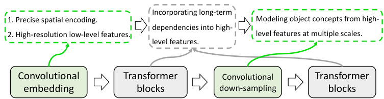
Fig. 1: The interleaved stem used in the encoder of nnFormer.
图 1: nnFormer编码器中使用的交错主干结构。
Former. Firstly, we put a light-weight convolutional embedding layer ahead of transformer blocks. In comparison to directly flattening raw pixels and applying 1D pre-processing in [17], the convolutional embedding layer encodes precise (i.e., pixellevel) spatial information and provides low-level yet highresolution 3D features. After the embedding block, transformer and convolutional down-sampling blocks are interleaved to fully entangle long-term dependencies with high-level and hierarchical object concepts at various scales, which helps improve the generalization ability and robustness of learned representations.
首先,我们在Transformer块前放置了一个轻量级的卷积嵌入层。与[17]中直接展平原始像素并应用一维预处理的方法相比,卷积嵌入层编码了精确(即像素级)的空间信息,并提供了低层次但高分辨率的3D特征。在嵌入块之后,Transformer和卷积下采样块交替出现,以充分交织长期依赖关系与多尺度的高层次分层对象概念,这有助于提高学习表示的泛化能力和鲁棒性。
The other contribution of nnFormer lies in proposing a computational-efficient way to leverage inter-slice dependencies. To be specific, nnFormer proposes to jointly use Local Volume-based Multi-head Self-attention (LV-MSA) and Global Volume-based Multi-head Self-attention (GV-MSA) to construct feature pyramids and provide sufficient receptive field for learning representations on both local and global 3D volumes, which are then aggregated to make predictions. Compared to the naive multi-head self-attention (MSA) [1], the proposed strategy can greatly reduce the computational complexity while producing competitive segmentation performance. Moreover, inspired by the attention mechanism used in the task of machine translation [1], we introduce skip attention to replace the atypical concatenation/summation operation in skip connections of U-Net like architecture, which further improves the segmentation results.
nnFormer的另一项贡献在于提出了一种计算高效的方法来利用切片间的依赖关系。具体而言,nnFormer提出联合使用基于局部体素的多头自注意力 (LV-MSA) 和基于全局体素的多头自注意力 (GV-MSA) 来构建特征金字塔,并为局部和全局3D体素上的表征学习提供足够的感受野,然后聚合这些特征进行预测。与朴素的多头自注意力 (MSA) [1] 相比,所提出的策略可以大大降低计算复杂度,同时产生具有竞争力的分割性能。此外,受机器翻译任务中使用的注意力机制 [1] 启发,我们引入跳跃注意力 (skip attention) 来替代类似U-Net架构跳跃连接中的非典型拼接/求和操作,从而进一步提升了分割结果。
To sum up, our contributions can be summarized as follows:
综上所述,我们的贡献可概括如下:
II. RELATED WORK
II. 相关工作
In this section, we mainly review methodologies that resort to transformers to improve segmentation results of medical images. Since most of them employ hybrid architecture of convolution and self-attention [1], we divide them into two categories based on whether the majority of the stem is convolutional or transformer-based.
在本节中,我们主要回顾利用Transformer提升医学图像分割效果的方法。由于多数方法采用卷积与自注意力 [1] 的混合架构,我们根据主干网络以卷积为主还是基于Transformer,将其分为两大类。
Convolution-based stem. TransUNet [11] first time applied transformer to improve the segmentation results of medical images. TransUNet treats the convnet as a feature extractor to generate a feature map for the input slice. Patch embedding is then applied to patches of feature maps in the bottleneck instead of raw images in ViT [2]. Concurrently, similar to TransUNet, Li et al. [20] proposed to use a squeezed attention block to regularize the self-attention modules of transformers and an expansion block to learn diversified representations for fundus images, which are all implemented in the bottleneck within convnets. TransFuse [13] introduced a BiFusion module to fuse features from the shallow convnet-based encoder and transformer-based segmentation network to make final predictions on 2D images. Compared to TransUNet, TransFuse mainly applied the self-attention mechanism to the input embedding layer to improve segmentation models on 2D images. Yun et al. [21] employed transformers to incorporate spectral information, which are entangled with spectral information encoded by convolutional features to address the problem of hyper spectral pathology. Xu et al. [22] extensively studied the trade-off between transformers and convnets and proposed a more efficient encoder named LeViT-UNet. Li et al. [23] presented a new up-sampling approach and incorporated it into the decoder of UNet to model long-term dependencies and global information for better reconstruction results. TransClaw U-Net [15] utilized transformers in UNet with more convolutional feature pyramids. Trans AttUNe t [16] explored the feasibility of applying transformer self attention with convolutional global spatial attention. Xie et al. [24] adopted transformers to capture long-term dependencies of multi-scale convolutional features from different layers of convnets. TransBTS [25] first utilized 3D convnets to extract volumetric spatial features and down-sample the input 3D images to produce hierarchical representations. The outputs of the encoder in TransBTS are then reshaped into a vector (i.e. token) and fed into transformers for global feature modeling, after which an ordinary convolutional decoder is appended to up-sample feature maps for the goal of reconstruction. Different from these approaches that directly employ convnets as feature extractors, our nnFormer functionally relies on convolutional and transformer-based blocks, which are interleaved to take advantages of each other.
基于卷积的骨干网络。TransUNet [11] 首次应用Transformer来提升医学图像的分割效果。TransUNet将卷积网络作为特征提取器,为输入切片生成特征图。随后在瓶颈层对特征图块进行块嵌入(patch embedding),而非像ViT [2]那样直接处理原始图像。与此同时,与TransUNet类似,Li等人[20]提出使用压缩注意力块来规范Transformer的自注意力模块,并通过扩展块学习眼底图像的多样化表征,这些操作均在卷积网络的瓶颈层实现。TransFuse [13]引入双向融合(BiFusion)模块,将基于浅层卷积网络的编码器特征与基于Transformer的分割网络特征相融合,最终完成二维图像的预测。相比TransUNet,TransFuse主要将自注意力机制应用于输入嵌入层,以改进二维图像的分割模型。Yun等人[21]采用Transformer整合光谱信息,这些信息与卷积特征编码的光谱信息相互纠缠,以解决高光谱病理学问题。Xu等人[22]深入研究了Transformer与卷积网络的权衡关系,提出名为LeViT-UNet的高效编码器。Li等人[23]提出新型上采样方法,并将其集成到UNet解码器中,以建模长程依赖和全局信息,获得更好的重建效果。TransClaw U-Net [15]在UNet中结合更多卷积特征金字塔来应用Transformer。TransAttUNet [16]探索了将Transformer自注意力与卷积全局空间注意力结合的可行性。Xie等人[24]采用Transformer捕捉卷积网络不同层级多尺度卷积特征的长程依赖。TransBTS [25]首次使用3D卷积网络提取体空间特征,并通过下采样输入3D图像生成层次化表征。TransBTS编码器的输出被重塑为向量(即token)并输入Transformer进行全局特征建模,最后接常规卷积解码器对特征图上采样以实现重建。与这些直接采用卷积网络作为特征提取器的方法不同,我们的nnFormer在功能上依赖相互交织的卷积块和Transformer块,以发挥各自优势。
Transformer-based stem. Valanarasu et al. [14] proposed a gated axial-attention model (i.e., MedT) which extends the existing convnet architecture by introducing an summation al control mechanism in the self-attention. Karimi et al. [17] removed the convolutional operations and built a 3D segmentation model based on transformers. The main idea is to first split the local volume block into 3D patches, which are then flattened and embedded to 1D sequences and passed to a ViT-like backbone to extract representations. SwinUNet [18] built a U-shape transformer-based segmentation model on top of transformer blocks in [3], where observable improvements were achieved. DS-TransUNet [19] further extended SwinUNet by adding one more encoder to handle multi-scale inputs and introduced a fusion module to effectively establish global dependencies between features of different scales through the self-attention mechanism. Compared to these transformerbased stems, nnFormer inherits the superiority of convolution in encoding precise spatial information and producing hierarchical representations that help model object concepts at various scales.
基于Transformer的骨干网络。Valanarasu等人[14]提出了一种门控轴向注意力模型(即MedT),通过在自注意力机制中引入求和控制机制来扩展现有卷积网络架构。Karimi等人[17]移除了卷积操作,构建了基于Transformer的3D分割模型。其核心思想是先将局部体块分割为3D补丁,然后将其展平并嵌入为1D序列,输入类似ViT的主干网络以提取表征。SwinUNet[18]在文献[3]的Transformer模块基础上构建了U型Transformer分割模型,取得了显著改进。DS-TransUNet[19]通过增加编码器处理多尺度输入,并引入融合模块利用自注意力机制有效建立不同尺度特征间的全局依赖关系,进一步扩展了SwinUNet。与这些基于Transformer的骨干网络相比,nnFormer继承了卷积在编码精确空间信息和生成多层次表征方面的优势,有助于建模不同尺度的对象概念。
III. METHOD
III. 方法
A. Overview
A. 概述
The overall architecture of nnFormer is presented in Figure 2, which maintains a similar U shape as that of U-Net [12] and mainly consists of three parts, i.e., the encoder, bottleneck and decoder. Concretely, the encoder involves one embedding layer, two local transformer blocks (each block contains two successive layers) and two down-sampling layers. Symmetrically, the decoder branch includes two transformer blocks, two up-sampling layers and the last patch expanding layer for making mask predictions. Besides, the bottleneck comprises one down-sampling layer, one up-sampling layer and three global transformer blocks for providing large receptive field to support the decoder. Inspired by U-Net [12], we add skip connections between corresponding feature pyramids of the encoder and decoder in a symmetrical manner, which helps to recover fine-grained details in the prediction. However, different from atypical skip connections that often use summation or concatenation operation, we introduce skip attention to bridge the gap between the encoder and decoder.
nnFormer的整体架构如图2所示,其保持了与U-Net [12]类似的U形结构,主要由三部分组成:编码器、瓶颈层和解码器。具体而言,编码器包含一个嵌入层、两个局部Transformer块(每个块包含两个连续层)和两个下采样层。对称地,解码器分支包含两个Transformer块、两个上采样层以及用于生成掩码预测的最后一个补丁扩展层。此外,瓶颈层包含一个下采样层、一个上采样层和三个全局Transformer块,用于提供大感受野以支持解码器。受U-Net [12]启发,我们以对称方式在编码器和解码器的对应特征金字塔之间添加跳跃连接,这有助于恢复预测中的细粒度细节。然而,不同于通常使用求和或拼接操作的非典型跳跃连接,我们引入了跳跃注意力来弥合编码器与解码器之间的差距。
In the following, we will demonstrate the forward procedure on Synapse. The forward pass on different datasets can be easily inferred based on the procedure on Synapse.
以下我们将演示在Synapse上的前向过程。基于Synapse上的流程,可以轻松推断出不同数据集上的前向传递。
B. Encoder
B. 编码器
The input of nnFormer is a 3D patch $\mathcal{X} \in~\mathcal{R}^{H\times W\times D}$ (usually randomly cropped from the original image), where $H,W$ and $D$ denote the height, width and depth of each input scan, respectively.
nnFormer的输入是一个3D图像块$\mathcal{X} \in~\mathcal{R}^{H\times W\times D}$(通常从原始图像中随机裁剪获得),其中$H,W$和$D$分别表示每个输入扫描的高度、宽度和深度。
The embedding layer. On Synapse, the embedding block is responsible for transforming each input scan $\mathcal{X}$ into a high-dimensional tensor $\begin{array}{r l r}{\gamma_{e}^{-}}&{{}\in}&{\mathrm{R}^{\frac{H}{4}\times\frac{W}{4}\times\frac{D}{2}\times C}}\end{array}$ , where $\frac{H}{4}\times\frac{W}{4}\times\frac{D}{2}$ represents the number of the patch tokens and C represents the sequence length (these numbers may slightly vary on different datasets). Different from ViT [2] and Swin Transformer [3] that use large convolutional kernels in the embedding block to extract features, we found that applying successive convolutional layers with small convolutional kernels bring more benefits in the initial stage, which could be explained from two perspectives, i.e., i) why applying successive convolutional layers and ii) why using small-sized kernels. For i), we use convolutional layers in the embedding block because they encode pixel-level spatial information, more precisely than patch-wise positional encoding used in transformers. For ii), compared to large-sized kernels, small kernel sizes help reduce computational complexity while providing equal-sized receptive field. As shown in Figure 2b, the embedding block consists of four convolutional layers whose kernel size is 3. After each convolutional layer (except the last one), one GELU [26] and one layer normalization [27] layers are appended. In practice, depending on the size of input patch, strides of convolution in the embedding block may accordingly vary.
嵌入层。在Synapse上,嵌入块负责将每个输入扫描$\mathcal{X}$转换为高维张量$\begin{array}{r l r}{\gamma_{e}^{-}}&{{}\in}&{\mathrm{R}^{\frac{H}{4}\times\frac{W}{4}\times\frac{D}{2}\times C}}\end{array}$,其中$\frac{H}{4}\times\frac{W}{4}\times\frac{D}{2}$表示补丁token的数量,C表示序列长度(这些数字在不同数据集上可能略有差异)。与ViT [2]和Swin Transformer [3]在嵌入块中使用大卷积核提取特征不同,我们发现应用连续的小卷积核卷积层在初始阶段能带来更多优势,这可以从两个角度解释:i) 为何使用连续卷积层;ii) 为何采用小尺寸卷积核。对于i),我们在嵌入块中使用卷积层是因为它们能编码像素级空间信息,比Transformer中使用的补丁级位置编码更精确。对于ii),与大尺寸卷积核相比,小卷积核有助于降低计算复杂度,同时提供同等大小的感受野。如图2b所示,嵌入块由四个卷积核大小为3的卷积层组成。每个卷积层后(除最后一层外)依次连接GELU [26]和层归一化[27]层。实际应用中,根据输入补丁尺寸,嵌入块中卷积的步长会相应调整。
Local Volume-based Multi-head Self-attention (LV-MSA). After the embedding layer, we pass the high-dimensional tensor $\mathcal{X}_{e}$ to transformer blocks. The main point behind is to fully entangle the captured long-term dependencies with the hierarchical object concepts at various scales produced by the down-sampling layers and the high-resolution spatial information encoded by the initial embedding layer. Compared to Swin Transformer [3], we compute self-attention within 3D local volumes (i.e., LV-MSA, Local Volume-based Multi-head Self-attention) instead of 2D local windows.
基于局部体积的多头自注意力机制 (LV-MSA)。经过嵌入层后,我们将高维张量 $\mathcal{X}_{e}$ 传递至Transformer模块。其核心思想在于:充分融合下采样层生成的多尺度层级物体概念、初始嵌入层编码的高分辨率空间信息,以及所捕获的长程依赖关系。与Swin Transformer [3] 相比,我们在3D局部体积内计算自注意力 (即LV-MSA) ,而非2D局部窗口。
Suppose that $\mathcal{X}{\mathrm{LV}}\in\mathcal{R}^{L\times C}$ represents the input of the local transformer block, $\mathcal{X}{\mathrm{LV}}$ would be first reshaped to $\hat{\mathcal{X}}{\mathrm{LV}}~\in$ $\mathbf{R}^{N_{\mathrm{LV}}\times N_{T}\times C}$ , where $N_{\mathrm{LV}}$ is a pre-defined number of 3D local volumes and $N_{T}=S_{H}\times S_{W}\times S_{D}$ denotes the number of patch tokens in each volume. ${S_{H},~S_{W},~S_{D}}$ stand for the size of local volume.
假设 $\mathcal{X}{\mathrm{LV}}\in\mathcal{R}^{L\times C}$ 表示局部Transformer块的输入,$\mathcal{X}{\mathrm{LV}}$ 会首先被重塑为 $\hat{\mathcal{X}}{\mathrm{LV}}~\in$ $\mathbf{R}^{N_{\mathrm{LV}}\times N_{T}\times C}$,其中 $N_{\mathrm{LV}}$ 是预定义的3D局部体积数量,$N_{T}=S_{H}\times S_{W}\times S_{D}$ 表示每个体积中的补丁Token数量。${S_{H},~S_{W},~S_{D}}$ 代表局部体积的尺寸。
As shown in Figure 3a, we follow [3] to conduct two successive transformer layers in each block, where the second layer can be regarded as a shifted version of the first layer (i.e., SLV-MSA). The main difference lies in that our computation is built on top of 3D local volumes instead of 2D local windows. The computational procedure can be summarized as follows:
如图 3a 所示, 我们遵循 [3] 在每个块中执行两个连续的 Transformer 层, 其中第二层可以视为第一层的移位版本 (即 SLV-MSA)。主要区别在于我们的计算是基于 3D 局部体积而非 2D 局部窗口进行的。计算过程可概括如下:
$$
\begin{array}{r l}&{\hat{\mathcal{X}}{\mathrm{LV}}^{l}=\mathrm{LV}{\bf M}\mathrm{SA}\left({\mathrm{Norm}\left(\mathcal{X}{\mathrm{LV}}^{l-1}\right)}\right)+\mathcal{X}{\mathrm{LV}}^{l-1},}\ &{\quad\mathcal{X}{\mathrm{LV}}^{l}={\mathrm{MLP}}\left({\mathrm{Norm}\left(\hat{\mathcal{X}}{\mathrm{LV}}^{l}\right)}\right)+\hat{\mathcal{X}}{\mathrm{LV}}^{l},}\ &{\hat{\mathcal{X}}{\mathrm{LV}}^{l+1}=\mathrm{SLV}{\bf M}\mathrm{SA}\left({\mathrm{Norm}\left(\mathcal{X}{\mathrm{LV}}^{l}\right)}\right)+\mathcal{X}{\mathrm{LV}}^{l},}\ &{\quad\mathcal{X}{\mathrm{LV}}^{l+1}={\mathrm{MLP}}\left({\mathrm{Norm}\left(\hat{\mathcal{X}}{\mathrm{LV}}^{l+1}\right)}\right)+\hat{\mathcal{X}}_{\mathrm{LV}}^{l+1}.}\end{array}
$$
$$
\begin{array}{r l}&{\hat{\mathcal{X}}{\mathrm{LV}}^{l}=\mathrm{LV}{\bf M}\mathrm{SA}\left({\mathrm{Norm}\left(\mathcal{X}{\mathrm{LV}}^{l-1}\right)}\right)+\mathcal{X}{\mathrm{LV}}^{l-1},}\ &{\quad\mathcal{X}{\mathrm{LV}}^{l}={\mathrm{MLP}}\left({\mathrm{Norm}\left(\hat{\mathcal{X}}{\mathrm{LV}}^{l}\right)}\right)+\hat{\mathcal{X}}{\mathrm{LV}}^{l},}\ &{\hat{\mathcal{X}}{\mathrm{LV}}^{l+1}=\mathrm{SLV}{\bf M}\mathrm{SA}\left({\mathrm{Norm}\left(\mathcal{X}{\mathrm{LV}}^{l}\right)}\right)+\mathcal{X}{\mathrm{LV}}^{l},}\ &{\quad\mathcal{X}{\mathrm{LV}}^{l+1}={\mathrm{MLP}}\left({\mathrm{Norm}\left(\hat{\mathcal{X}}{\mathrm{LV}}^{l+1}\right)}\right)+\hat{\mathcal{X}}_{\mathrm{LV}}^{l+1}.}\end{array}
$$
Here, $l$ stands for the layer index. MLP is an abbreviation for multi-layer perceptron. The computational complexity of LV-MSA on a volume of $h\times w\times d$ patches is:
这里,$l$ 代表层索引。MLP 是多层感知机 (multi-layer perceptron) 的缩写。LV-MSA 在 $h\times w\times d$ 个补丁上的计算复杂度为:
$$
\Omega(\mathrm{LV-MSA})=4h w d C^{2}+2S_{H}S_{W}S_{D}h w d C.
$$
$$
\Omega(\mathrm{LV-MSA})=4h w d C^{2}+2S_{H}S_{W}S_{D}h w d C.
$$
SLV-MSA displaces the 3D local volume used in LV-MSA by $\begin{array}{c c}{\left(\left\lfloor\frac{S_{H}}{2}\right\rfloor,\left\lfloor\frac{S_{\bar{W}}}{2}\right\rfloor,\left\lfloor\frac{S_{D}}{2}\right\rfloor\right)}\end{array}$ to introduce more interactions between different local volumes. In practice, SLV-MSA has the similar computational complexity as that of LV-MSA.
SLV-MSA通过将LV-MSA中使用的3D局部体积位移 $\begin{array}{c c}{\left(\left\lfloor\frac{S_{H}}{2}\right\rfloor,\left\lfloor\frac{S_{\bar{W}}}{2}\right\rfloor,\left\lfloor\frac{S_{D}}{2}\right\rfloor\right)}\end{array}$ 来引入不同局部体积之间更多的交互。实际上,SLV-MSA的计算复杂度与LV-MSA相似。
The query-key-value (QKV) attention [1] in each 3D local volume can be computed as follows:
每个3D局部体积中的查询-键-值 (QKV) 注意力 [1] 可按如下方式计算:
$$
\mathrm{Attention}(Q,K,V)=\mathrm{softmax}\left(\frac{Q K^{T}}{\sqrt{d_{k}}}+B\right)V,
$$
$$
\mathrm{Attention}(Q,K,V)=\mathrm{softmax}\left(\frac{Q K^{T}}{\sqrt{d_{k}}}+B\right)V,
$$
where $Q,K,V\in\mathcal{R}^{N_{T}\times d_{k}}$ denote the query, key and value matrices. $B\in\mathcal{R}^{N_{T}}$ is the relative position encoding. In practice, we first initialize a smaller-sized position matrix $\hat{\boldsymbol{B}}\in\mathcal{R}^{(2S_{H}-1)\times(2S_{W}-1)\times(2S_{D}-1)}$ and take corresponding values from $\hat{B}$ to build a larger position matrix $B$ .
其中 $Q,K,V\in\mathcal{R}^{N_{T}\times d_{k}}$ 表示查询矩阵、键矩阵和值矩阵。$B\in\mathcal{R}^{N_{T}}$ 是相对位置编码。实际应用中,我们首先初始化一个较小尺寸的位置矩阵 $\hat{\boldsymbol{B}}\in\mathcal{R}^{(2S_{H}-1)\times(2S_{W}-1)\times(2S_{D}-1)}$,然后从 $\hat{B}$ 中提取对应值来构建更大的位置矩阵 $B$。
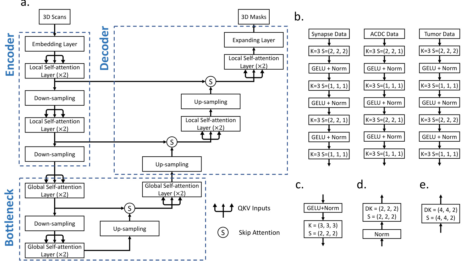
Fig. 2: Architecture of nnFormer. In (a), we show the overall architecture of nnFormer. In (b), we present more details of the embedding layers on three publicly available datasets. In (c), (d), (e), we display how to implement the down-sampling, up-sampling and expanding layers, respectively. In practice, the architecture may slightly vary depending on the input scan size. In (b)-(e), K denotes the convolutional kernel size, DK stands for the de convolutional kernel size and S represents the stride. Norm refers to the layer normalization strategy.
图 2: nnFormer架构。(a)展示了nnFormer的整体架构。(b)呈现了三个公开数据集上嵌入层的更多细节。(c)、(d)、(e)分别展示了如何实现下采样层、上采样层和扩展层。实际应用中,架构可能因输入扫描尺寸而略有差异。(b)-(e)中,K表示卷积核大小,DK代表反卷积核大小,S代表步长。Norm指代层归一化策略。
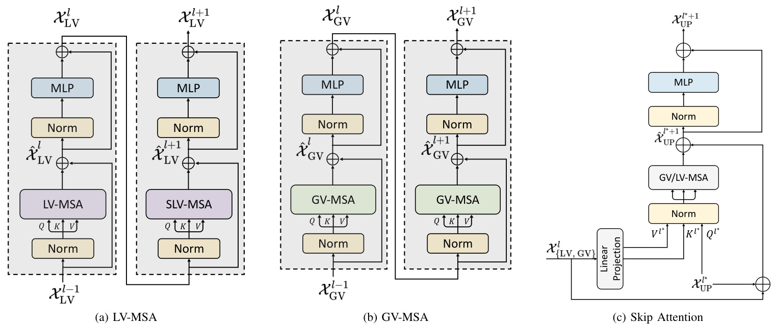
Fig. 3: Three types of attention mechanism in nnFormer. Norm denotes the layer normalization method. MLP is the abbreviation for multi-layer perceptron, which is a two-layer neural network in practice.
图 3: nnFormer中的三种注意力机制类型。Norm表示层归一化方法。MLP是多层感知机 (multi-layer perceptron) 的缩写,实际中是一个两层的神经网络。
The down-sampling layer. We found that by replacing the patch merging operation in [3] with straightforward strided convolution, nnFormer can provide more improvements on volumetric image segmentation. The intuition behind is that convolutional down-sampling produces hierarchical representations that help model object concepts at multiple scales. As displayed in Figure 2c, in most cases, the down-sampling layer involves a strided convolution operation where the stride is set to 2 in all dimensions. However, in practice, the stride with respect to specific dimension can be set to 1 as the number of slices is limited in this dimension and over-down-sampling (i.e., using a large down-sampling stride) can be harmful.
下采样层。我们发现,通过将[3]中的补丁合并操作替换为简单的跨步卷积(strided convolution),nnFormer能在体积图像分割任务上实现更显著的性能提升。其原理在于卷积下采样能生成层次化表征,有助于模型在多尺度上理解目标概念。如图2c所示,多数情况下该层采用跨步卷积操作,各维度步长(stride)均设为2。但实际应用中,针对切片数量有限的维度,可将对应步长设为1以避免过度下采样(即使用过大下采样步长)带来的负面影响。
(c) ACDC
| nnFormer | nnUNet | |
|---|---|---|
| Spacing | [1.0, 1.0, 1.0] | [1.0,1.0,1.0] |
| Median shape | 138× 170 × 138 | 138× 170 × 138 |
| Crop size | 128 × 128 × 128 | 128 × 128 × 128 |
| Batch size | 2 | 2 |
| DS Str. | [2,2,2],[2,2,2],[2,2,2], [2,2,2],[2,2,2] | [2,2,2],[2,2,2],[2,2,2], [2,2,2],[2,2,2] |
| (a) Tumor | ||
| nnFormer | nnUNet | |
| Spacing | [0.76, 0.76,3] | [0.76, 0.76, 3] |
| Median shape Crop size | 512 × 512 × 148 | 512 × 512 × 148 192 × 192 × 48 |
| Batch size | 128 × 128 × 64 2 | 2 |
| DS Str. | [2,2,2],[2,2,1],[2,2,2], [2,2,2],[2,2,2] (b) Synapse | [2,2,1],[2,2,2],[2,2,2], [2,2,2],[2,2,1] |
| nnFormer | nnUNet | |
| Spacing | [1.52, 1.52, 6.35] | [1.52,1.52,6.35] |
| Median shape | 246 × 213 × 13 | 246 × 213 × 13 |
| Crop size Batch size | 160 × 160 × 14 4 | 256 × 224 × 14 4 |
| DS Str. | [2,2,1],[2,2,1],[2,2,1], [2,2,2],[2,2,2] | [2,2,1],[2,2,1],[2,2,2], [2,2,1],[2,2,1] |
| (c) ACDC |
TABLE I: Network configurations of our nnFormer and nnUNet on three public datasets. We only report the downsampling stride (abbreviated as DS Str.) as the corresponding up-sampling stride can be easily inferred according to symmetrical down-sampling operations. Note that the network configuration of nnUNet is automatically determined based on pre-defined hand-crafted rules (for self-adaptation).
表 I: 我们提出的nnFormer和nnUNet在三个公开数据集上的网络配置。这里仅报告下采样步长(简称DS Str.),因为对应的上采样步长可根据对称的下采样操作轻松推导。需要注意的是,nnUNet的网络配置是基于预定义的手工规则(用于自适应)自动确定的。
C. Bottleneck
C. 瓶颈
The original vision transformer (i.e., ViT) [2] employs the naive 2D multi-head self-attention mechanism. In this paper, we extend it to a 3D version (as shown in Figure 3b), whose computational complexity can be formulated as follows:
原始视觉Transformer (即ViT) [2] 采用了基础的2D多头自注意力机制。本文将这一机制扩展至3D版本 (如图 3b 所示) ,其计算复杂度可表述如下:
$$
\Omega({\mathrm{GV}}{-}{\mathrm{MSA}})=4h w d C^{2}+2(h w d)^{2}C.
$$
$$
\Omega({\mathrm{GV}}{-}{\mathrm{MSA}})=4h w d C^{2}+2(h w d)^{2}C.
$$
Compared to (2), it is obvious that GV-MSA requires much more computational resources when ${h,w,d}$ are relatively larger (e.g., an order of magnitude larger) than ${S_{H},S_{W},S_{D}}$ . In fact, this is exactly the reason why we use local transformer blocks in the encoder, which are designed to handle large-sized inputs efficiently with the local self-attention mechanism.
与(2)相比,显然当${h,w,d}$比${S_{H},S_{W},S_{D}}$大得多(例如大一个数量级)时,GV-MSA需要更多的计算资源。事实上,这正是我们在编码器中使用局部Transformer块的原因,这些模块通过局部自注意力机制高效处理大规模输入。
However, in the bottleneck, ${h,w,d}$ already become much smaller after several down-sampling layers, making the product of them, i.e. hwd, , have a similar size to that of $S_{H}S_{W}S_{D}$ . This creates the condition for applying GV-MSA, which is able to provide larger receptive field compared to LV-MSA and large receptive field has been proven to be beneficial in different applications [28]–[31]. In practice, we use three global transformer blocks (i.e., six GV-MSA layers) in the bottleneck to provide sufficient receptive field to the decoder.
然而,在瓶颈结构中,经过多次下采样层后,${h,w,d}$已经变得非常小,使得它们的乘积(即hwd)与$S_{H}S_{W}S_{D}$的尺寸相近。这为应用GV-MSA(全局视觉多头自注意力)创造了条件,与LV-MSA相比,GV-MSA能够提供更大的感受野,而大感受野已被证明在不同应用中具有优势[28]–[31]。在实际应用中,我们在瓶颈部分使用了三个全局Transformer块(即六层GV-MSA)来为解码器提供足够的感受野。
D. Decoder
D. 解码器
The architecture of two transformer blocks in the decoder is highly symmetrical to those in the encoder. In contrast to the down-sampling blocks, we employ strided de convolution to up-sample low-resolution feature maps to high-resolution ones, which in turn are merged with representations from the encoder via skip attention to capture both semantic and fine-grained information. Similar to up-sampling blocks, the last patch expanding block also takes the de convolutional operation to produce final mask predictions.
解码器中两个Transformer块的结构与编码器中的高度对称。与下采样块不同,我们采用跨步反卷积将低分辨率特征图上采样至高分辨率,再通过跳跃注意力与编码器的表征合并,以同时捕获语义和细粒度信息。与上采样块类似,最后的补丁扩展块同样采用反卷积操作生成最终的掩码预测。
Skip Attention. Atypical skip connections in convnets [12, 32] adapt either concatenation or summation to incorporate more information. Inspired by the machine translation task in [1], we propose to replace the concatenation/summation with an attention mechanism, which is named as Skip Attention in this paper. To be specific, the output of the $l$ -th transformer block of the encoder, i.e., $\chi_{{\mathrm{LV,GV}}}^{l}$ , is transformed and split into a key matrix $K^{l^{}}$ and a value matrix $V^{l^{*}}$ after the linear projection (i.e, a one-layer neural network):
跳跃注意力 (Skip Attention) 。卷积网络中的非典型跳跃连接 [12, 32] 采用拼接或求和方式来融合更多信息。受 [1] 中机器翻译任务的启发,我们提出用注意力机制替代拼接/求和操作,本文将其命名为跳跃注意力。具体而言,编码器第 $l$ 个 Transformer 块的输出 $\chi_{{\mathrm{LV,GV}}}^{l}$ 经过线性投影 (即单层神经网络) 后,被转换并拆分为键矩阵 $K^{l^{}}$ 和值矩阵 $V^{l^{*}}$:
$$
\begin{array}{r}{K^{l^{}},V^{l^{*}}=\mathrm{LP}(\mathcal{X}_{{\mathrm{LV},\mathrm{GV}}}^{l}),}\end{array}
$$
$$
\begin{array}{r}{K^{l^{}},V^{l^{*}}=\mathrm{LP}(\mathcal{X}_{{\mathrm{LV},\mathrm{GV}}}^{l}),}\end{array}
$$
where LP stands for the linear projection. Accordingly, $\chi_{\mathrm{UP}}^{l^{}}$ , the output feature maps after the $l^{}$ -th up-sampling layer of the decoder, is treated as the query $Q^{l^{}}$ . Then, we can conduct LV/GV-MSA on $Q^{l^{}},K^{l^{}}$ and $V^{l^{}}$ in the decoder like what we have done in (3), i.e.,
其中LP表示线性投影。相应地,解码器中第 $l^{}$ 个上采样层后的输出特征图 $\chi_{\mathrm{UP}}^{l^{}}$ 被视为查询 $Q^{l^{}}$。然后,我们可以像在(3)中那样,在解码器中对 $Q^{l^{}},K^{l^{}}$ 和 $V^{l^{*}}$ 进行LV/GV-MSA操作,即
$$
\mathrm{Attention}({Q^{l}}^{},{K^{l}}^{},{V^{l}}^{})=\mathrm{softmax}\left(\frac{{Q^{l}}^{}({K^{l}}^{})^{T}}{\sqrt{d_{k}^{l^{}}}}+{B^{l^{}}}\right){V^{l}}^{*},
$$
$$
\mathrm{Attention}({Q^{l}}^{},{K^{l}}^{},{V^{l}}^{})=\mathrm{softmax}\left(\frac{{Q^{l}}^{}({K^{l}}^{})^{T}}{\sqrt{d_{k}^{l^{}}}}+{B^{l^{}}}\right){V^{l}}^{*},
$$
where $l^{}$ denotes the layer index. $d_{k}^{l^{}}$ and $B^{l^{*}}$ have the same meaning as those in (3), whose sizes can be easily inferred, accordingly.
其中 $l^{}$ 表示层索引。$d_{k}^{l^{}}$ 和 $B^{l^{*}}$ 的含义与(3) 式中相同,其大小可相应推断得出。
IV. EXPERIMENTS
IV. 实验
For thoroughly comparing nnFormer to previous convnetand transformer-based architecture, we conduct experiments on three datasets/tasks: the brain tumor segmentation task in Medical Segmentation Decathlon (MSD) [36], Synapse multiorgan segmentation [37] and Automatic Cardiac Diagnosis Challenge (ACDC) [38]. For each experiment, we repeat it for ten times and report their average results. We also calculate p-values to demonstrate the significance of nnFormer.
为了全面比较nnFormer与之前基于卷积网络和Transformer的架构,我们在三个数据集/任务上进行了实验:医学分割十项全能赛(MSD) [36]中的脑肿瘤分割任务、Synapse多器官分割[37]以及自动心脏诊断挑战赛(ACDC) [38]。每个实验重复十次并报告其平均结果,同时计算p值以证明nnFormer的显著性。
Brain tumor segmentation using MRI scans. This task consists of $484~\mathrm{MRI}$ images, each of which includes four channels, i.e., FLAIR, T1w, T1gd and T2w. The data was acquired from 19 different institutions and contained a subset of the data used in the 2016 and 2017 Brain Tumor Segmentation (BraTS) challenges [39]. The corresponding
使用MRI扫描进行脑肿瘤分割。该任务包含484张MRI图像,每张图像包含四个通道,即FLAIR、T1w、T1gd和T2w。数据来自19个不同机构,并包含了2016年和2017年脑肿瘤分割(BraTS)挑战赛[39]中所用数据的子集。对应的
TABLE II: Comparison with transformer-based models on brain tumor segmentation. The evaluation metrics are HD95 (mm) and DSC in $(%)$ . Best results are bolded while second best are underlined. Experimental results of baselines are from [34]. We calculate the $\mathsf{p}$ -values between the average performance of our nnFormer and the best performing baseline in both metrics.
表 II: 基于Transformer的脑肿瘤分割模型对比。评估指标为HD95 (mm) 和DSC (%) 。最优结果加粗显示,次优结果加下划线。基线实验结果来自[34]。我们计算了nnFormer平均性能与各指标最优基线之间的p值。
| 方法 | HD95↓ 平均 | DSC↑ 平均 | HD95↓ WT | DSC↑ WT | HD95↓ ET | DSC↑ ET | HD95↓ TC | DSC↑ TC |
|---|---|---|---|---|---|---|---|---|
| SETR NUP [33] | 13.78 | 63.7 | 14.419 | 69.7 | 11.72 | 54.4 | 15.19 | 66.9 |
| SETR PUP [33] | 14.01 | 63.8 | 15.245 | 69.6 | 11.76 | 54.9 | 15.023 | 67.0 |
| SETR MLA [33] | 13.49 | 63.9 | 15.503 | 69.8 | 10.24 | 55.4 | 14.72 | 66.5 |
| TransUNet [11] | 12.98 | 64.4 | 14.03 | 70.6 | 10.42 | 54.2 | 14.5 | 68.4 |
| TransBTS [25] | 9.65 | 69.6 | 10.03 | 77.9 | 9.97 | 57.4 | 8.95 | 73.5 |
| CoTr w/o CNN encoder [24] | 11.22 | 64.4 | 11.49 | 71.2 | 9.59 | 52.3 | 12.58 | 69.8 |
| CoTr [24] | 9.70 | 68.3 | 9.20 | 74.6 | 9.45 | 55.7 | 10.45 | 74.8 |
| UNETR [34] | 8.82 | 71.1 | 8.27 | 78.9 | 9.35 | 58.5 | 8.85 | 76.1 |
| Our nnFormer P-values | 4.05 | 86.4 | 3.80 | 91.3 | 3.87 < 1e-2 (HD95), < 1e-2 (DSC) | 81.8 | 4.49 | 86.0 |
| 方法 | 平均 HD95↓ | 平均 DSC↑ | Aotra | 胆囊 | 左肾 | 右肾 | 肝脏 | 胰腺 | 脾脏 | 胃 |
|---|---|---|---|---|---|---|---|---|---|---|
| ViT[2]+CUP[11] | 36.11 | 67.86 | 70.19 | 45.10 | 74.70 | 67.40 | 91.32 | 42.00 | 81.75 | 70.44 |
| R50-ViT[2]+CUP[11] | 32.87 | 71.29 | 73.73 | 55.13 | 75.80 | 72.20 | 91.51 | 45.99 | 81.99 | 73.95 |
| TransUNet[11] | 31.69 | 77.48 | 87.23 | 63.16 | 81.87 | 77.02 | 94.08 | 55.86 | 85.08 | 75.62 |
| TransUNet[11] | 84.36 | 90.68 | 71.99 | 86.04 | 83.71 | 95.54 | 73.96 | 88.80 | 84.20 | |
| SwinUNet[18] | 21.55 | 79.13 | 85.47 | 66.53 | 83.28 | 79.61 | 94.29 | 56.58 | 90.66 | 76.60 |
| TransClawU-Net[15] | 26.38 | 78.09 | 85.87 | 61.38 | 84.83 | 79.36 | 94.28 | 57.65 | 87.74 | 73.55 |
| LeVit-UNet-384s[22] | 16.84 | 78.53 | 87.33 | 62.23 | 84.61 | 80.25 | 93.11 | 59.07 | 88.86 | 72.76 |
| MISSFormer[35] | 18.20 | 81.96 | 86.99 | 68.65 | 85.21 | 82.00 | 94.41 | 65.67 | 91.92 | 80.81 |
| UNETR[34] | 22.97 | 79.56 | 89.99 | 60.56 | 85.66 | 84.80 | 94.46 | 59.25 | 87.81 | 73.99 |
| Our nnFormer | 10.63 | 86.57 | 92.04 | 70.17 | 86.57 | 86.25 | 96.84 | 83.35 | 90.51 | 86.83 |
| P值 | <1e-2(HD95), <1e-2(DSC) |
TABLE III: Comparison with transformer-based models on multi-organ segmentation (Synapse). The evaluation metrics are HD95 (mm) and DSC in $(%)$ . Best results are bolded while second best are underlined. $\bigtriangledown$ denotes TransUNet uses larger inputs, whose size is $512\times512$ . The $\mathsf{p}$ -values are calculated based on the average performance of our nnFormer and the best performing baseline in both metrics.
表 III: 基于Transformer的多器官分割模型对比(Synapse数据集)。评估指标为HD95(mm)和DSC($%$)。最优结果加粗显示,次优结果加下划线。$\bigtriangledown$表示TransUNet采用更大输入尺寸($512\times512$)。$\mathsf{p}$值根据nnFormer平均性能与各指标最优基线的对比计算得出。
| 方法 | 平均 | RV | Myo | LV |
|---|---|---|---|---|
| VIT-CUP [2] | 81.45 | 81.46 | 70.71 | 92.18 |
| R50-VIT-CUP [2] | 87.57 | 86.07 | 81.88 | 94.75 |
| TransUNet[11] | 89.71 | 88.86 | 84.54 | 95.73 |
| SwinUNet [18] | 90.00 | 88.55 | 85.62 | 95.83 |
| LeViT-UNet-384s [22] | 90.32 | 89.55 | 87.64 | 93.76 |
| UNETR[34] | 88.61 | 85.29 | 86.52 | 94.02 |
| nnFormer | 92.06 | 90.94 | 89.58 | 95.65 |
| P值 | < 1e-2 (DSC) |
TABLE IV: Comparison with transformer-based models on automatic cardiac diagnosis (ACDC). The evaluation metric is DSC $(%)$ . Best results are bolded while second best are underlined. The default evaluation metric is DSC, based on which we calculate the p-value.
表 IV: 基于Transformer的模型在自动心脏诊断(ACDC)任务上的对比。评估指标为DSC $(%)$。最佳结果加粗显示,次优结果加下划线。默认评估指标为DSC,并基于此计算p值。
target ROIs were the three tumor sub-regions, namely edema (ED), enhancing tumor (ET), and non-enhancing tumor (NET). To be consistent with those results reported in UNETR [34], we display the experimental results of the whole tumor (WT), enhancing tumor (ET) and tumor core (TC) when comparing our nnFormer with transformer-based models. For the split of data, we follow the instruction of UNETR, where ratios of training/validation/test sets are $80%$ , $15%$ and $5%$ , respectively. As above, we use both HD95 and Dice score as evaluation metrics.
目标感兴趣区域(ROI)为三个肿瘤子区域,即水肿区(ED)、强化肿瘤区(ET)和非强化肿瘤区(NET)。为与UNETR [34]报告的结果保持一致,在比较nnFormer与其他基于Transformer的模型时,我们展示全肿瘤(WT)、强化肿瘤(ET)和肿瘤核心(TC)的实验结果。数据划分遵循UNETR的方案,训练集/验证集/测试集的比例分别为$80%$、$15%$和$5%$。如上所述,我们同时采用HD95和Dice分数作为评估指标。
Synapse for multi-organ CT segmentation. This dataset includes 30 cases of abdominal CT scans. Following the split used in [11], 18 cases are extracted to build the training set while the rest 12 cases are used for testing. We report the model performance evaluated with the $95%$ Hausdorff Distance (HD95) and Dice score (DSC) on 8 abdominal organs, which are aorta, gallbladder, spleen, left kidney, right kidney, liver, pancreas and stomach1.
用于多器官CT分割的Synapse数据集。该数据集包含30例腹部CT扫描。按照[11]中的划分方式,18例用于构建训练集,其余12例用于测试。我们报告模型在8个腹部器官(主动脉、胆囊、脾脏、左肾、右肾、肝脏、胰腺和胃1)上的性能评估结果,采用95%豪斯多夫距离(HD95)和Dice相似系数(DSC)作为指标。
ACDC for automated cardiac diagnosis. ACDC involves 100 patients, with the cavity of the right ventricle, the myocardium of the left ventricle and the cavity of the left ventricle to be segmented. Each case’s labels involve left ventricle (LV), right ventricle (RV) and myocardium (MYO). The dataset is split into 70 training samples, 10 validation samples and 20 test samples. The evaluation metrics include
用于自动化心脏诊断的ACDC。ACDC包含100名患者的数据,需要分割右心室腔、左心室心肌和左心室腔。每个病例的标注包含左心室(LV)、右心室(RV)和心肌(MYO)。数据集划分为70个训练样本、10个验证样本和20个测试样本。评估指标包括
both HD95 and Dice score2.
HD95和Dice分数
A. Implementation details
A. 实现细节
We run all experiments based on Python 3.6, PyTorch 1.8.1 and Ubuntu 18.04. All training procedures have been performed on a single NVIDIA 2080 GPU with 11GB memory. The initial learning rate is set to 0.01 and we employ a “poly” decay strategy as described in Equation 7. The default optimizer is SGD where we set the momentum to 0.99. The weight decay is set to 3e-5. We utilize both cross entropy loss and dice loss by simply summing them up. The number of training epochs (i.e., max epoch in Equation 7) is 1000 and one epoch contains 250 iterations. The number of heads of multi-head self-attention used in different encoder stages is [6, 12, 24, 48] on Synapse. In the rest two datasets, the number of heads becomes [3, 6, 12, 24].
我们基于Python语言 3.6、PyTorch 1.8.1和Ubuntu 18.04运行所有实验。所有训练过程均在单张11GB显存的NVIDIA 2080 GPU上完成。初始学习率设为0.01,并采用公式7所述的"poly"衰减策略。默认优化器为SGD,动量设为0.99,权重衰减设为3e-5。我们通过简单相加的方式同时使用交叉熵损失和dice损失。训练周期数(即公式7中的max epoch)为1000,每个周期包含250次迭代。在Synapse数据集上,不同编码器阶段使用的多头自注意力头数分别为[6, 12, 24, 48]。在其余两个数据集中,头数变为[3, 6, 12, 24]。
Pre-processing and augmentation strategies. All images will be first resampled to the same target spacing. Augmentations such as rotation, scaling, gaussian noise, gaussian blur, brightness and contrast adjust, simulation of low resolution, gamma augmentation and mirroring are applied in the given order during the training process.
预处理与增强策略。所有图像将首先重采样至相同目标间距。在训练过程中按给定顺序应用旋转、缩放、高斯噪声、高斯模糊、亮度对比度调整、低分辨率模拟、伽马增强和镜像等增强方法。
Deep supervision. We also add deep supervision during the training stage. Specifically, the output of each stage in the decoder is passed to the final expanding block, where cross entropy loss and dice loss would be applied. In practice, given the prediction of one typical stage, we down-sample the ground truth segmentation mask to match the prediction’s resolution. Thus, the final training objective function is the sum of all losses at three resolutions:
深度监督。我们在训练阶段也加入了深度监督。具体来说,解码器每个阶段的输出都会传递到最终的扩展块,并在此处应用交叉熵损失和dice损失。实际操作中,给定某一典型阶段的预测结果时,我们会将真实分割掩码下采样以匹配预测分辨率。因此,最终的训练目标函数是三个分辨率下所有损失的总和:
$$
\mathcal{L}{a l l}=\alpha_{1}\mathcal{L}{{H,:W,:D}}+\alpha_{2}\mathcal{L}{{\frac{H}{4},:\frac{W}{4},:\frac{D}{2}}}+\alpha_{3}\mathcal{L}_{{\frac{H}{8},:\frac{W}{8},:\frac{D}{4}}}.
$$
$$
\mathcal{L}{a l l}=\alpha_{1}\mathcal{L}{{H,:W,:D}}+\alpha_{2}\mathcal{L}{{\frac{H}{4},:\frac{W}{4},:\frac{D}{2}}}+\alpha_{3}\mathcal{L}_{{\frac{H}{8},:\frac{W}{8},:\frac{D}{4}}}.
$$
Here, $\alpha_{{1,2,3}}$ denote the magnitude factors for losses in different resolutions. In practice, $\alpha_{{1,2,3}}$ halve with each decrease in resolution, leading to $\alpha_{2} =~\frac{\alpha_{1}}{2}$ and $\begin{array}{l c r}{{\alpha_{3}}}\end{array}=\frac{\alpha_{1}}{4}$ . Finally, all weight factors are normalized to 1.
此处,$\alpha_{{1,2,3}}$ 表示不同分辨率下的损失幅度因子。实际应用中,$\alpha_{{1,2,3}}$ 随分辨率每降低一级而减半,即 $\alpha_{2} =~\frac{\alpha_{1}}{2}$ 且 $\begin{array}{l c r}{{\alpha_{3}}}\end{array}=\frac{\alpha_{1}}{4}$。最终所有权重因子均归一化为1。
Network configurations. In Table I, we display network configurations of experiments on all three datasets. Compared to nnUNet, in nnFormer, better segmentation results can be achieved with smaller-sized input patches.
网络配置。表1展示了我们在所有三个数据集上的实验网络配置。与nnUNet相比,nnFormer能以更小尺寸的输入块(patches)获得更好的分割效果。
B. Comparison with transformer-based methodologies
B. 与基于Transformer的方法对比
Brain tumor segmentation. Table II presents experimental results of all models on the task of brain tumor segmentation. Our nnFormer achieves the lowest HD95 and the highest DSC scores in all classes. Moreover, nnFormer is able to surpass the second best method, i.e., UNETR, by large margins in both evaluation metrics. For instance, nnFormer outperforms UNETR by over $4.5\mathrm{mm}$ in average HD95 and nearly 10 percents in DSC of each class. In comparison to previous transformer-based methods, nnFormer shows more strength in HD95 than in DSC.
脑肿瘤分割。表 II 展示了所有模型在脑肿瘤分割任务上的实验结果。我们的 nnFormer 在所有类别中均取得了最低的 HD95 和最高的 DSC 分数。此外,nnFormer 在两项评估指标上均大幅领先第二名方法 UNETR。例如,nnFormer 在平均 HD95 上比 UNETR 低超过 $4.5\mathrm{mm}$,在各类别的 DSC 上高出近 10%。与之前基于 Transformer 的方法相比,nnFormer 在 HD95 上的优势比 DSC 更显著。

Fig. 4: Visualization of segmentation results on three wellestablished datasets. We mainly compare nnFormer against nnUNet and UNETR. In addition to segmentation results, we also provide ground truth masks for better comparison.
图 4: 在三个成熟数据集上的分割结果可视化。我们主要将 nnFormer 与 nnUNet 和 UNETR 进行对比。除分割结果外,我们还提供了真实标注掩膜以便更好比较。
Multi-organ segmentation (Synapse). As shown in Table III, we make experiments on Synapse and to compare our nnFormer against a variety of transformer-based approaches. As we can see, the best performing methods are LeViT-UNet384s [22] and TransUNet [11]. LeViT-UNet-384s achieves an average HD95 of $16.84\mathrm{ mm}$ while TransUNet produces an average DSC of $84.36%$ . In comparison, our nnFormer is able to outperform LeViT-UNet-384s and TransUNet by over $6~\mathrm{mm}$ and 2 percents in average HD95 and DSC, respectively, which are quite impressive improvements on Synapse. To be specific, nnFormer achieves the highest DSC in six organs, including aotra, kidney (left), kidney (right), liver, pancreas and stomach. Compared to previous transformer-based methods, nnFormer is more advantageous in segmentation pancreas and stomach, both of which are difficult to delineate using past segmentation models.
多器官分割 (Synapse)。如表 III 所示,我们在 Synapse 数据集上进行了实验,并将 nnFormer 与多种基于 Transformer 的方法进行了比较。可以看出,表现最好的方法是 LeViT-UNet384s [22] 和 TransUNet [11]。LeViT-UNet-384s 的平均 HD95 为 $16.84\mathrm{ mm}$,而 TransUNet 的平均 DSC 为 $84.36%$。相比之下,我们的 nnFormer 在平均 HD95 和 DSC 上分别比 LeViT-UNet-384s 和 TransUNet 高出超过 $6~\mathrm{mm}$ 和 2 个百分点,这在 Synapse 数据集上是相当显著的改进。具体而言,nnFormer 在六个器官(主动脉、左肾、右肾、肝脏、胰腺和胃)上取得了最高的 DSC。与之前基于 Transformer 的方法相比,nnFormer 在分割胰腺和胃方面更具优势,这两个器官在过去的分割模型中难以准确勾勒。
(a) Brain tumor segmentation
(a) 脑肿瘤分割
| 方法 | 平均 | WT | ET | TC | ED | NET |
|---|---|---|---|---|---|---|
| HD95√ | DSC↑ | HD95√ | DSC↑ | HD95√ | DSC↑ | |
| nnUNet[40] | 4.60 | 81.87 | 3.64 | 91.99 | 4.06 | 80.97 |
| OurnnFormer | 4.42 | 82.02 | 3.80 | 91.26 | 3.87 | 81.80 |
| P-values | ||||||
| nnAvg | 4.09 | 82.65 | 3.43 | 92.33 | 3.69 | 82.26 |
(b) Multi-organ segmentation (Synapse)
(b) 多器官分割 (Synapse)
| 方法 | 平均值 | 主动脉 | 胆囊 | 左肾 | 右肾 | 肝脏 | 胰腺 | 脾脏 | 胃 | ||||||||
|---|---|---|---|---|---|---|---|---|---|---|---|---|---|---|---|---|---|
| HD95↓DSC↑HD95↓DSC↑ | HD95↓DSC↑ | HD95↓DSC↑ | HD95↓DSC↑ | HD95↓DSC↑B | HD95↓DSC↑ | HD95↓DSC↑HD95↓DSC↑ | |||||||||||
| nnUNet [40] | 10.78 | 86.99 5.91 | 93.01 | 15.19 | 71.77 | 18.60 | 85.57 | 6.44 | 88.18 | 1.62 | 97.23 | 4.52 | 83.01 | 24.34 | 91.86 | 9.58 | 85.26 |
| OurnnFormer | 10.63 | 86.57 | 11.38 92.04 | 11.55 | 70.17 | 18.09 | 86.57 | 12.76 | 86.25 | 2.00 | 96.84 | 3.72 | 83.35 | 16.92 | 90.51 | 8.58 86.83 | |
| P值 | 2e-2 | (HD95), 7.7e-2 | (DSC) | ||||||||||||||
| nnAvg | 7.70 | 87.51 | 5.90 | 93.11 | 8.63 72.08 | 18.42 | 86.20 | 8.56 | 87.76 | 1.63 | 97.20 | 3.64 | 84.21 | 9.42 | 91.94 | 5.41 | 87.60 |
TABLE V: Comparison with nnUNet on three public datasets. nnAvg means that we simply average the predictions of nnUNet and nnFormer. Color green denotes the target result of nnAvg is the best among all three approaches. Besides, we also highlight the best results between nnUNet and nnFormer in bold font. We calculate p-values between the average performance of nnUNet and our nnFormer in both metrics on three public datasets.
(c) Automated cardiac diagnosis (ACDC)
表 V: 在三个公开数据集上与nnUNet的对比。nnAvg表示我们简单平均了nnUNet和nnFormer的预测结果。绿色标注表示nnAvg的目标结果是三种方法中最好的。此外,我们还用粗体标出了nnUNet和nnFormer之间的最佳结果。我们计算了nnUNet和我们的nnFormer在三个公开数据集上两项指标的平均性能之间的p值。
| 方法 | HD95√ | DSC↑ | HD95√ | DSC↑ | HD95√ | DSC↑ | HD95√ | DSC↑ |
|---|---|---|---|---|---|---|---|---|
| nnUNet [40] | 1.15 | 91.61 | 1.31 | 90.24 | 1.06 | 89.24 | 1.09 | 95.36 |
| OurnnFormer | 1.12 | 92.06 | 1.23 | 90.94 | 1.04 | 89.58 | 1.09 | 95.65 |
| P-values | 2e-2 (HD95), < 1e-2 (DSC) | |||||||
| nnAvg | 1.10 | 92.15 | 1.19 | 91.03 | 1.04 | 89.75 | 1.06 | 95.68 |
(c) 自动化心脏诊断 (ACDC)
TABLE VI: Investigation of the impact of different modules used in nnFormer. PM and PE denote the patch merging and patch embedding strategies used in swin transformer [3]. Conv. Embed. and Conv. Down. represent our convolutional embedding and down-sampling layers, respectively. Skip Att. refers to the proposed skip attention mechanism. $1\times\mathrm{LV{-}M S A}$ in lines 0-2 means that each transformer block contains one transformer layer and each layer consists of one LV-MSA. $1\times\mathrm{GV}.$ -MSA in lines 3-4 denotes that we replace LV-MSA in the bottleneck with GV-MSA. $1\times\mathrm{SLV{-}M S A}$ and $2\times\mathrm{GV}{\cdot}\mathrm{MSA}$ in line 5 mean that we increase the number of transformer layers in each transformer block from one to two. To be specific, in the encoder/decoder, each transformer block contains $1{\times}\mathrm{LV{-}M S A}$ and $1\times$ SLV-MSA while in the bottleneck, there are $2\times\mathrm{GV}{-}\mathrm{MSA}$ in each block.
表 VI: nnFormer中不同模块影响的探究。PM和PE表示swin transformer [3]中使用的patch merging和patch embedding策略。Conv. Embed.和Conv. Down.分别代表我们的卷积嵌入和下采样层。Skip Att.指提出的跳跃注意力机制。0-2行中的$1\times\mathrm{LV{-}M S A}$表示每个transformer块包含一个transformer层,每层由一个LV-MSA组成。3-4行中的$1\times\mathrm{GV}.$-MSA表示我们在瓶颈处用GV-MSA替换了LV-MSA。第5行中的$1\times\mathrm{SLV{-}M S A}$和$2\times\mathrm{GV}{\cdot}\mathrm{MSA}$表示我们将每个transformer块中的transformer层数从一层增加到两层。具体来说,在编码器/解码器中,每个transformer块包含$1{\times}\mathrm{LV{-}M S A}$和$1\times$SLV-MSA,而在瓶颈处,每个块中有$2\times\mathrm{GV}{-}\mathrm{MSA}$。
| # | 模型 | 平均 | RV | Myo | LV |
|---|---|---|---|---|---|
| 0 | 1xLV-MSA+PM[3]+PE[3] | 90.55 | 88.59 | 88.47 | 94.60 |
| 1 | 1xLV-MSA+PM[3]+Conv.Embed. | 90.97 | 88.94 | 88.84 | 95.13 |
| 2 | 1xLV-MSA+Conv.Down.+Conv.Embed. | 91.26 | 89.70 | 89.04 | 95.04 |
| 3 | 1xLV-MSA+1xGV-MSA+Conv.Down.+Conv.Embed. | 91.46 | 89.82 | 89.17 | 95.39 |
| 4 | 1xLV-MSA+1xGV-MSA+Conv.Down.+Conv.Embed.+Skip Att. | 91.85 | 90.41 | 89.50 | 95.63 |
| 5 | 1xLV-MSA+1xSLV-MSA+2xGV-MSA+Conv.Down.+Conv.Embed.+SkipAtt. | 92.06 | 90.94 | 89.58 | 95.65 |
Automated cardiac diagnosis (ACDC). Table IV displays experimental results on ACDC. We can see that the best transformer-based model is LeViT-UNet-384s, whose average DSC is slightly higher than SwinUNet while TransUNet and SwinUNet are more capable of handling the delineation of the left ventricle (LV). In contrast, nnFormer surpasses LeViT-UNet-384s in all classes and by nearly 1.7 percents in average DSC, which again verifies its advantages over past transformer-based approaches.
自动化心脏诊断 (ACDC) 。表 IV 展示了 ACDC 上的实验结果。可以看出,基于 Transformer 的最佳模型是 LeViT-UNet-384s,其平均 DSC 略高于 SwinUNet,而 TransUNet 和 SwinUNet 更擅长处理左心室 (LV) 的轮廓描绘。相比之下,nnFormer 在所有类别上都超越了 LeViT-UNet-384s,平均 DSC 高出近 1.7%,这再次验证了其相较于以往基于 Transformer 方法的优势。
Statistical significance. In Table II, III and IV, we employ independent two-sample t-test to calculate p-values between the average performance of our nnFormer and the best performing baseline in both HD95 and DSC. The null hypothesis is that our nnFormer has no advantage over the best performing baseline. As we can see, on all three public datasets, nnFormer produces p-values smaller than 1e-2 under both HD95 and DSC, which indicate strong evidence against the null hypothesis. Thus, nnFormer shows significant improvements over previous transformer-based methods on three different tasks.
统计显著性。在表II、III和IV中,我们采用独立双样本t检验计算nnFormer与HD95和DSC两项指标最优基线的平均性能间p值。零假设为nnFormer相比最优基线不具有优势。结果显示,在全部三个公开数据集上,nnFormer在HD95和DSC指标下获得的p值均小于1e-2,这为拒绝零假设提供了强有力证据。因此,nnFormer在三种不同任务上均显示出对既往基于Transformer方法的显著改进。
C. Comparison with nnUNet and Discussion
C. 与nnUNet的对比和讨论
In this section, we compare nnFormer with nnUNet, which has been recognized as one of the most powerful 3D medical image segmentation models [40].
在本节中,我们将nnUNet与nnFormer进行对比。nnUNet已被公认为最强大的3D医学图像分割模型之一 [40]。
Results. In Table V, we display the class-specific results in both HD95 and DSC metrics to make a thorough comparison. To be specific, from the perspective of the class-specific HD95 results, nnFormer outperforms nnUNet in 11 out of 16 categories. In the class-specific DSC, nnFormer outperforms nnUNet in 9 out of 16 categories. Thus, it seems that nnFormer is more advantageous under HD95, which means nnFormer may better delineate the object boundary. From the view of the average performance, we can see that nnFormer often achieves better average performance. For example, nnFormer outperforms nnUNet on all three public datasets with lower HD95 results, while performing better than nnUNet on two out of three datasets with higher DSC results.
结果。在表 V 中,我们展示了 HD95 和 DSC 指标的类别特异性结果以进行全面比较。具体而言,从类别特异性 HD95 结果来看,nnFormer 在 16 个类别中有 11 个优于 nnUNet。在类别特异性 DSC 方面,nnFormer 在 16 个类别中有 9 个优于 nnUNet。因此,nnFormer 在 HD95 指标下似乎更具优势,这意味着 nnFormer 可能更好地描绘了对象边界。从平均性能来看,nnFormer 通常能取得更好的平均表现。例如,nnFormer 在所有三个公开数据集上的 HD95 结果均优于 nnUNet,同时在三个数据集中的两个上以更高的 DSC 结果优于 nnUNet。
Statistical significance. To further verify the significance of nnFormer over nnUNet, we also calculate the p-values between the average performance of nnFormer and nnUNet. Similar to what we have done in Table II, we provide two p-values based on HD95 and DSC on three public datasets, respectively. The most obvious observation is that nnFormer achieves p-values smaller than 0.05 in HD95 on three public datasets. These results suggest that nnFormer is the first choice when HD95 is treated as the primary evaluation metric. Besides, the p-values based on DSC on tumor and multi-organ segmentation $(>0.05)$ imply that nnFormer is a model comparable to nnUNet, while the results on ACDC demonstrate the significance of nnFormer. In conclusion, nnFormer has slight advantages over nnUNet under DSC.
统计显著性。为进一步验证nnFormer相对于nnUNet的显著性,我们还计算了二者平均性能的p值。与表2中的做法类似,我们基于三个公开数据集的HD95和DSC分别提供了两组p值。最显著的观察结果是:nnFormer在三个公开数据集的HD95指标上均获得小于0.05的p值。这些结果表明,当以HD95作为主要评估指标时,nnFormer是首选方案。此外,基于肿瘤和多器官分割DSC的p值$(>0.05)$表明nnUNet与nnFormer性能相当,而ACDC数据集的结果则凸显了nnFormer的显著优势。综上所述,在DSC指标下nnFormer较nnUNet具有轻微优势。
Model ensembling. Besides single model performance, we also investigate the diversity between nnFormer and nnUNet, which is a crucial factor in model ensembling. Somewhat surprisingly, we found that by simply averaging the predictions of nnFormer and nnUNet (i.e., nnAvg in Table V), it can already boost the overall performance by large margins. For instance, nnAvg achieves the best results in all classes under HD95 and DSC on tumor segmentation. Moreover, nnAvg brings nearly $30%$ improvements on Synapse when the evaluation metric is HD95. These results indicate that nnFormer and nnUNet are highly complementary to each other.
模型集成。除了单一模型性能外,我们还研究了nnFormer与nnUNet之间的差异性——这是模型集成的关键因素。令人惊讶的是,我们发现仅通过对nnFormer和nnUNet的预测结果取平均值(即表V中的nnAvg),就能显著提升整体性能。例如,在肿瘤分割任务中,nnAvg在HD95和DSC指标下所有类别都取得了最佳结果。此外,当评估指标为HD95时,nnAvg在Synapse数据集上带来了近30%的性能提升。这些结果表明nnFormer与nnUNet具有高度互补性。
D. Ablation study
D. 消融实验
Table VI displays our ablation study results towards different modules in nnFormer. For simplicity, we made experiments on ACDC and used DSC as the default evaluation metric.
表 VI 展示了我们对 nnFormer 中不同模块的消融研究结果。为简化实验,我们在 ACDC 数据集上进行测试,并默认使用 DSC 作为评估指标。
The most basic baseline in Table VI (line 0) consists of LV-MSA (but without SLV-MSA), the patch merging and embedding layers used in [3]. We can see that such combination can already achieve a higher average DSC than LeViT-UNet-38 [22], which is the best performing baseline in Table IV. We firstly replaced the patch embedding layer, which is implemented with large kernel size and convolutional stride, with our proposed volume embedding layer, i.e., successive convolutional layers with small kernel size and convolutional stride. We found that the introduced convolutional embedding layer improves the average DSC by approximate 0.4 percents.
表 VI (第 0 行) 中最基础的基线由 LV-MSA (但不包含 SLV-MSA) 以及 [3] 中使用的块合并和嵌入层组成。可以看出,这种组合的平均 DSC 已经高于 LeViT-UNet-38 [22] (表 IV 中表现最佳的基线)。我们首先将采用大卷积核和卷积步长的块嵌入层替换为提出的体积嵌入层 (即连续的小卷积核和步长的卷积层),发现引入的卷积嵌入层将平均 DSC 提升了约 0.4%。
Next, we removed the patch merging layer and added our convolutional down-sampling layer. We found such simple replacement can further boost the overall performance by 0.3 percents. Then, we replaced LV-MSA in the bottleneck with GV-MSA, where we observed 0.2-percent improvements. This phenomenon indicates that providing sufficient larger receptive field can be beneficial to the segmentation task. Afterwards, we use skip attention to replace traditional concatenation/summation operations. Somewhat surprisingly, we found that the skip attention is able to boost the overall performance by 0.4 percents, which demonstrates that the skip attention may serve as an alternative choice other than traditional skip connections. Last but not the least, we investigate adding more transformer layers to each transformer block by cascading an SLV-MSA layer with every LV-MSA layer as in Swin Transformer and doubling the number of global self-attention layers. We found that introducing more transformer layers does bring more improvements to the overall performance as it entangles more long-range dependencies into the learned volume representations.
接下来,我们移除了补丁合并层并添加了卷积下采样层。发现这种简单替换能进一步提升整体性能0.3%。随后,我们将瓶颈结构中的LV-MSA替换为GV-MSA,观察到0.2%的性能提升。这一现象表明,提供足够大的感受野对分割任务具有增益效果。之后,我们用跳跃注意力机制替代传统的拼接/求和操作。出乎意料的是,跳跃注意力能使整体性能提升0.4%,这说明该机制可以成为传统跳跃连接之外的新选择。最后,我们通过在每个Transformer块中叠加SLV-MSA层(如Swin Transformer那样)并倍增全局自注意力层数量,来研究增加更多Transformer层的效果。发现引入更多Transformer层确实能通过增强长程依赖关系来提升学习到的体表示质量,从而持续改善整体性能。
E. Visualization of segmentation results
E. 分割结果的可视化
In Figure 4, we visualize some segmentation results of our nnFormer, nnUNet and UNETR on three public datasets. Compared to UNETR, our nnFormer can greatly reduce the number of false positive predictions. One typical example is the fifth example on ACDC. We can see that UNETR produces a large number of wrong right ventricle pixels outside the myocardium. In contrast, our nnFormer generates no prediction of right ventricle outside the myocardium, which demonstrates that nnFormer is more disc rim i native than UNETR on ACDC.
图4展示了我们的nnFormer、nnUNet和UNETR在三个公共数据集上的部分分割结果可视化。与UNETR相比,nnFormer能显著减少假阳性预测数量。典型案例如ACDC数据集的第五个样本所示:UNETR在心肌外区域错误预测了大量右心室像素,而nnFormer则完全未在心肌外生成右心室预测,这表明nnFormer在ACDC数据集上比UNETR更具判别力。
On the other hand, we observe that nnUNet displays very competitive segmentation results, much better than UNETR in nearly all examples. However, we still find that nnFormer maintains clear advantages over nnUNet, one of which is that nnFormer is better at dealing with the boundary. In fact, this phenomenon has been reflected in Table VI, where nnFormer is significantly better than nnUNet when HD95 is the default evaluation metric. In Figure 4, we can also observe some evidences. For instance, in the second example on Synapse, nnFormer captures the shape of the left kidney and stomach better than nnUNet. Also, in the third example on brain tumor segmentation, nnUNet misses a major part of the non-enhancing tumor enclosed by the edema. These results verify that our nnFormer has the potential to be treated as an alternative to nnUNet.
另一方面,我们观察到nnUNet展现出极具竞争力的分割结果,在几乎所有案例中都明显优于UNETR。然而,nnFormer仍保持对nnUNet的明显优势,其中一点是nnFormer更擅长处理边界问题。这一现象已在表VI中得到体现:当采用HD95作为默认评估指标时,nnFormer显著优于nnUNet。图4中也能观察到相关证据:例如在Synapse数据集的第二个案例中,nnFormer对左肾和胃部轮廓的捕捉优于nnUNet;在脑肿瘤分割的第三个案例中,nnUNet漏检了被水肿包裹的非增强肿瘤主体。这些结果验证了我们的nnFormer具备成为nnUNet替代方案的潜力。
V. CONCLUSION
V. 结论
In this paper, we present a 3D transformer, nnFormer, for volumetric image segmentation. nnFormer is constructed on top of an interleaved stem of convolution and self-attention. Convolution helps encode precise spatial information and builds hierarchical object concepts. For self-attention, nnFormer employs three types of attention mechanism to entangle long-range dependencies. Specifically, local and global volume-based self-attention focus on constructing feature pyramids and providing large receptive field. Skip attention is responsible for bridging the gap between the encoder and decoder. Experiments show that nnFormer maintains great advantages over previous transformer-based models in both HD95 and DSC. Compared to nnUNet, nnFormer is significantly better in HD95 while producing comparable results in DSC. More importantly, we demonstrate that nnFormer and nnUNet can be beneficial to each other in model ensembling, where the simple averaging operation can already produce great improvements.
本文提出了一种用于体积图像分割的3D Transformer模型nnFormer。该模型构建在卷积与自注意力交错的基础架构上:卷积用于编码精确的空间信息并构建层次化物体概念;自注意力部分采用三种注意力机制捕获长程依赖关系,其中局部和全局体积自注意力负责构建特征金字塔并提供大感受野,跳跃注意力则用于弥合编码器与解码器之间的差距。实验表明,nnFormer在HD95和DSC指标上均显著优于此前基于Transformer的模型。与nnUNet相比,nnFormer在HD95指标上优势明显,同时保持相当的DSC性能。更重要的是,我们证明nnFormer与nnUNet在模型集成中能形成优势互补,仅通过简单平均操作即可获得显著提升。