U-Net: Convolutional Networks for Biomedical Image Segmentation
U-Net: 用于生物医学图像分割的卷积网络
Abstract. There is large consent that successful training of deep networks requires many thousand annotated training samples. In this paper, we present a network and training strategy that relies on the strong use of data augmentation to use the available annotated samples more efficiently. The architecture consists of a contracting path to capture context and a symmetric expanding path that enables precise localization. We show that such a network can be trained end-to-end from very few images and outperforms the prior best method (a sliding-window convolutional network) on the ISBI challenge for segmentation of neuronal structures in electron microscopic stacks. Using the same network trained on transmitted light microscopy images (phase contrast and DIC) we won the ISBI cell tracking challenge 2015 in these categories by a large margin. Moreover, the network is fast. Segmentation of a $512\mathrm{x512}$ image takes less than a second on a recent GPU. The full implementation (based on Caffe) and the trained networks are available at http://lmb.informatik.uni-freiburg.de/people/ronneber/u-net.
摘要。人们普遍认为,深度网络的训练成功需要成千上万的标注训练样本。本文提出了一种网络及训练策略,通过充分利用数据增强技术来更高效地利用现有标注样本。该架构包含捕捉上下文的收缩路径和实现精确定位的对称扩展路径。我们证明,这种网络可以从极少量图像端到端训练,并在ISBI电子显微镜堆栈神经元结构分割挑战中超越了先前最佳方法(滑动窗口卷积网络)。使用相同网络在透射光学显微镜图像(相差干涉和DIC)上训练后,我们以显著优势赢得了2015年ISBI细胞追踪挑战赛相应类别。此外,该网络速度极快,在现代GPU上分割$512\mathrm{x512}$图像仅需不到一秒。完整实现(基于Caffe)及训练好的网络详见http://lmb.informatik.uni-freiburg.de/people/ronneber/u-net。
1 Introduction
1 引言
In the last two years, deep convolutional networks have outperformed the state of the art in many visual recognition tasks, e.g. [7,3]. While convolutional networks have already existed for a long time [8], their success was limited due to the size of the available training sets and the size of the considered networks. The breakthrough by Krizhevsky et al. [7] was due to supervised training of a large network with 8 layers and millions of parameters on the ImageNet dataset with 1 million training images. Since then, even larger and deeper networks have been trained [12].
近两年,深度卷积网络在许多视觉识别任务中超越了现有最佳技术 [7,3]。尽管卷积网络早已存在 [8],但由于可用训练集的规模和所考虑网络的规模限制,其成功一直有限。Krizhevsky等人 [7] 的突破在于使用包含100万张训练图像的ImageNet数据集,对有800万参数、8层的大型网络进行了监督训练。此后,更大更深的网络相继被训练出来 [12]。
The typical use of convolutional networks is on classification tasks, where the output to an image is a single class label. However, in many visual tasks, especially in biomedical image processing, the desired output should include localization, i.e., a class label is supposed to be assigned to each pixel. Moreover, thousands of training images are usually beyond reach in biomedical tasks. Hence, Ciresan et al. [1] trained a network in a sliding-window setup to predict the class label of each pixel by providing a local region (patch) around that pixel as input. First, this network can localize. Secondly, the training data in terms of patches is much larger than the number of training images. The resulting network won the EM segmentation challenge at ISBI 2012 by a large margin.
卷积网络的典型应用是分类任务,即对图像输出单个类别标签。然而,在许多视觉任务中,尤其是生物医学图像处理领域,期望的输出应包含定位信息,也就是需要为每个像素分配类别标签。此外,生物医学任务通常难以获取数千张训练图像。为此,Ciresan等人[1]采用滑动窗口方法训练网络,通过输入目标像素周围的局部区域(图像块)来预测每个像素的类别标签。这种设计首先实现了定位功能,其次以图像块为单位的训练数据量远大于原始图像数量。该网络以显著优势赢得了2012年ISBI大会的EM分割挑战赛。
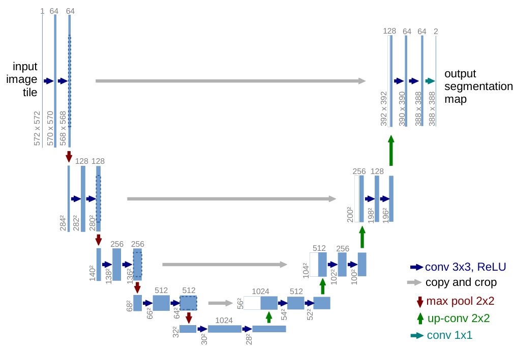
Fig. 1. U-net architecture (example for $32\mathrm{x32}$ pixels in the lowest resolution). Each blue box corresponds to a multi-channel feature map. The number of channels is denoted on top of the box. The x-y-size is provided at the lower left edge of the box. White boxes represent copied feature maps. The arrows denote the different operations.
图 1: U-net架构 (最低分辨率为 $32\mathrm{x32}$ 像素的示例)。每个蓝色框对应一个多通道特征图,通道数标注在框体上方,x-y尺寸标注在框体左下角。白色框表示复制的特征图,箭头表示不同的操作。
Obviously, the strategy in Ciresan et al. [1] has two drawbacks. First, it is quite slow because the network must be run separately for each patch, and there is a lot of redundancy due to overlapping patches. Secondly, there is a trade-off between localization accuracy and the use of context. Larger patches require more max-pooling layers that reduce the localization accuracy, while small patches allow the network to see only little context. More recent approaches [11,4] proposed a classifier output that takes into account the features from multiple layers. Good localization and the use of context are possible at the same time.
显然,Ciresan等人[1]提出的策略存在两个缺点。首先,由于需要对每个图像块单独运行网络且重叠块导致大量冗余计算,该方法速度较慢。其次,定位精度与上下文利用之间存在矛盾:较大的图像块需要更多最大池化层(max-pooling layers)从而降低定位精度,而较小图像块又限制了网络感知上下文的能力。最新研究[11,4]提出通过融合多层特征的分类器输出方案,实现了定位精度与上下文利用的同步优化。
In this paper, we build upon a more elegant architecture, the so-called “fully convolutional network” [9]. We modify and extend this architecture such that it works with very few training images and yields more precise segmentation s; see Figure 1. The main idea in [9] is to supplement a usual contracting network by successive layers, where pooling operators are replaced by upsampling operators. Hence, these layers increase the resolution of the output. In order to localize, high resolution features from the contracting path are combined with the upsampled output. A successive convolution layer can then learn to assemble a more precise output based on this information.
在本文中,我们基于一种更优雅的架构——所谓的"全卷积网络 (fully convolutional network)" [9]进行构建。我们对该架构进行修改和扩展,使其能够在极少量训练图像下工作,并产生更精确的分割结果(参见图1)。文献[9]的核心思想是通过连续层来补充常规的收缩网络,其中池化算子被上采样算子取代。因此,这些层提高了输出的分辨率。为了实现定位,收缩路径中的高分辨率特征与上采样输出相结合。随后,连续的卷积层可以基于这些信息学习组装出更精确的输出。
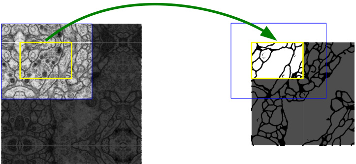
Fig. 2. Overlap-tile strategy for seamless segmentation of arbitrary large images (here segmentation of neuronal structures in EM stacks). Prediction of the segmentation in the yellow area, requires image data within the blue area as input. Missing input data is extrapolated by mirroring
图 2: 用于任意大图像无缝分割的重叠平铺策略 (此处为EM堆栈中神经元结构的分割)。黄色区域的分割预测需要蓝色区域内的图像数据作为输入。缺失的输入数据通过镜像进行外推
One important modification in our architecture is that in the upsampling part we have also a large number of feature channels, which allow the network to propagate context information to higher resolution layers. As a consequence, the expansive path is more or less symmetric to the contracting path, and yields a u-shaped architecture. The network does not have any fully connected layers and only uses the valid part of each convolution, i.e., the segmentation map only contains the pixels, for which the full context is available in the input image. This strategy allows the seamless segmentation of arbitrarily large images by an overlap-tile strategy (see Figure 2). To predict the pixels in the border region of the image, the missing context is extrapolated by mirroring the input image. This tiling strategy is important to apply the network to large images, since otherwise the resolution would be limited by the GPU memory.
我们架构中的一个重要改进是在上采样部分也设置了大量特征通道,这使得网络能将上下文信息传递到更高分辨率的层级。因此,扩展路径与收缩路径基本对称,从而形成了U型架构。该网络不含任何全连接层,仅使用每个卷积的有效部分,即分割图仅包含输入图像中具备完整上下文的像素。这种策略通过重叠切片技术(见图2)实现了任意尺寸图像的无缝分割。为预测图像边缘区域的像素,缺失的上下文通过镜像输入图像进行外推。这种切片策略对处理大尺寸图像至关重要,否则分辨率将受限于GPU显存容量。
As for our tasks there is very little training data available, we use excessive data augmentation by applying elastic deformations to the available training images. This allows the network to learn invariance to such deformations, without the need to see these transformations in the annotated image corpus. This is particularly important in biomedical segmentation, since deformation used to be the most common variation in tissue and realistic deformations can be simulated efficiently. The value of data augmentation for learning invariance has been shown in Do sov it ski y et al. [2] in the scope of unsupervised feature learning.
由于我们的任务可用的训练数据非常少,我们通过对现有训练图像施加弹性变形来进行过度的数据增强。这使得网络能够学习对此类变形的不变性,而无需在标注图像库中看到这些变换。这在生物医学分割中尤为重要,因为变形曾是组织中最常见的变化,且可以高效模拟真实的变形。数据增强对学习不变性的价值已在Dosovitskiy等人[2]的无监督特征学习研究中得到证实。
Another challenge in many cell segmentation tasks is the separation of touching objects of the same class; see Figure 3. To this end, we propose the use of a weighted loss, where the separating background labels between touching cells obtain a large weight in the loss function.
许多细胞分割任务中的另一个挑战是分离同一类别中相互接触的物体;见图3。为此,我们提出使用加权损失函数,其中相互接触细胞之间的分隔背景标签在损失函数中获得较大权重。
The resulting network is applicable to various biomedical segmentation problems. In this paper, we show results on the segmentation of neuronal structures in EM stacks (an ongoing competition started at ISBI 2012), where we outperformed the network of Ciresan et al. [1]. Furthermore, we show results for cell segmentation in light microscopy images from the ISBI cell tracking challenge 2015. Here we won with a large margin on the two most challenging 2D transmitted light datasets.
生成的网络适用于多种生物医学分割问题。本文展示了在EM堆栈中神经元结构分割的结果(始于ISBI 2012的持续竞赛),我们的表现优于Ciresan等人的网络[1]。此外,我们还展示了2015年ISBI细胞追踪挑战赛中光镜图像细胞分割的结果,在两个最具挑战性的2D透射光数据集上以显著优势获胜。
2 Network Architecture
2 网络架构
The network architecture is illustrated in Figure 1. It consists of a contracting path (left side) and an expansive path (right side). The contracting path follows the typical architecture of a convolutional network. It consists of the repeated application of two 3x3 convolutions (unpadded convolutions), each followed by a rectified linear unit (ReLU) and a 2x2 max pooling operation with stride 2 for down sampling. At each down sampling step we double the number of feature channels. Every step in the expansive path consists of an upsampling of the feature map followed by a 2x2 convolution (“up-convolution”) that halves the number of feature channels, a concatenation with the correspondingly cropped feature map from the contracting path, and two 3x3 convolutions, each followed by a ReLU. The cropping is necessary due to the loss of border pixels in every convolution. At the final layer a 1x1 convolution is used to map each 64- component feature vector to the desired number of classes. In total the network has 23 convolutional layers.
网络架构如图 1 所示。它由收缩路径 (left side) 和扩展路径 (right side) 组成。收缩路径遵循卷积网络的典型架构,包含重复应用的两个 3x3 卷积 (unpadded convolutions),每个卷积后接一个线性修正单元 (ReLU) 和步长为 2 的 2x2 最大池化操作进行下采样。每次下采样时我们将特征通道数量翻倍。扩展路径中的每个步骤包含对特征图进行上采样,接着是一个 2x2 卷积 ("up-convolution") 将特征通道数减半,与收缩路径中相应裁剪的特征图进行拼接,以及两个 3x3 卷积,每个卷积后接一个 ReLU。由于每次卷积会丢失边缘像素,裁剪是必要的操作。在最后一层使用 1x1 卷积将 64 维特征向量映射到目标类别数。该网络共包含 23 个卷积层。
To allow a seamless tiling of the output segmentation map (see Figure 2), it is important to select the input tile size such that all 2x2 max-pooling operations are applied to a layer with an even x- and y-size.
为了实现输出分割图的无缝平铺 (参见图 2),必须选择适当的输入图块尺寸,确保所有2x2最大池化操作都在x和y维度为偶数的层上执行。
3 Training
3 训练
The input images and their corresponding segmentation maps are used to train the network with the stochastic gradient descent implementation of Caffe [6]. Due to the unpadded convolutions, the output image is smaller than the input by a constant border width. To minimize the overhead and make maximum use of the GPU memory, we favor large input tiles over a large batch size and hence reduce the batch to a single image. Accordingly we use a high momentum (0.99) such that a large number of the previously seen training samples determine the update in the current optimization step.
输入图像及其对应的分割图用于训练网络,采用Caffe [6] 的随机梯度下降实现。由于未填充卷积操作,输出图像会比输入图像小一个固定的边界宽度。为降低开销并最大化利用GPU内存,我们优先选择大尺寸输入图块而非大批次量,因此将批次大小缩减为单张图像。相应地,我们采用高动量值 (0.99) ,使得当前优化步骤的更新由大量先前见过的训练样本决定。
The energy function is computed by a pixel-wise soft-max over the final feature map combined with the cross entropy loss function. The soft-max is defined as $\begin{array}{r}{p_{k}(\mathbf{x})=\exp(a_{k}(\mathbf{x}))/\left(\sum_{k^{\prime}=1}^{K}\exp(a_{k^{\prime}}(\mathbf{x}))\right)}\end{array}$ where $a_{k}(\mathbf{x})$ denotes the activation in feature channel $k$ at the pixel position $\mathbf{x}\in\varOmega$ with $\varOmega\subset\mathbb{Z}^{2}$ . $K$ is the number of classes and $p_{k}(\mathbf{x})$ is the approximated maximum-function. I.e. $p_{k}(\mathbf{x})\approx1$ for the $k$ that has the maximum activation $a_{k}(\mathbf x)$ and $p_{k}(\mathbf{x})\approx0$ for all other $k$ . The cross entropy then penalizes at each position the deviation of $p_{\ell(\mathbf{x})}(\mathbf{x})$ from 1 using
能量函数通过结合交叉熵损失函数对最终特征图进行逐像素soft-max计算得到。soft-max定义为 $\begin{array}{r}{p_{k}(\mathbf{x})=\exp(a_{k}(\mathbf{x}))/\left(\sum_{k^{\prime}=1}^{K}\exp(a_{k^{\prime}}(\mathbf{x}))\right)}\end{array}$ ,其中 $a_{k}(\mathbf{x})$ 表示在像素位置 $\mathbf{x}\in\varOmega$ ( $\varOmega\subset\mathbb{Z}^{2}$ ) 处特征通道 $k$ 的激活值。 $K$ 是类别总数, $p_{k}(\mathbf{x})$ 为近似最大值函数。即当 $k$ 对应的激活值 $a_{k}(\mathbf x)$ 最大时 $p_{k}(\mathbf{x})\approx1$ ,其余情况 $p_{k}(\mathbf{x})\approx0$ 。交叉熵通过以下方式惩罚每个位置上 $p_{\ell(\mathbf{x})}(\mathbf{x})$ 与1的偏差:
$$
E=\sum_{\mathbf{x}\in\Omega}w(\mathbf{x})\log(p_{\ell(\mathbf{x})}(\mathbf{x}))
$$
$$
E=\sum_{\mathbf{x}\in\Omega}w(\mathbf{x})\log(p_{\ell(\mathbf{x})}(\mathbf{x}))
$$
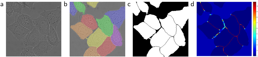
Fig. 3. HeLa cells on glass recorded with DIC (differential interference contrast) microscopy. (a) raw image. (b) overlay with ground truth segmentation. Different colors indicate different instances of the HeLa cells. (c) generated segmentation mask (white: foreground, black: background). (d) map with a pixel-wise loss weight to force the network to learn the border pixels.
图 3: 使用DIC (微分干涉差) 显微镜记录的玻璃上的HeLa细胞。(a) 原始图像。(b) 与真实分割叠加的效果图。不同颜色表示不同的HeLa细胞实例。(c) 生成的分割掩码 (白色: 前景, 黑色: 背景)。(d) 带有逐像素损失权重的映射图, 用于强制网络学习边界像素。
where $\ell:\varOmega\to{1,\dots,K}$ is the true label of each pixel and $w:\varOmega\to\mathbb{R}$ is a weight map that we introduced to give some pixels more importance in the training.
其中 $\ell:\varOmega\to{1,\dots,K}$ 是每个像素的真实标签,$w:\varOmega\to\mathbb{R}$ 是我们引入的权重图,用于在训练中赋予某些像素更高的重要性。
We pre-compute the weight map for each ground truth segmentation to compensate the different frequency of pixels from a certain class in the training data set, and to force the network to learn the small separation borders that we introduce between touching cells (See Figure 3c and d).
我们预先计算每个真实分割的权重图,以补偿训练数据集中某类像素的不同频率,并强制网络学习我们在接触细胞之间引入的小分隔边界(见图3c和d)。
The separation border is computed using morphological operations. The weight map is then computed as
分离边界通过形态学运算计算得出。随后权重图计算为
$$
w(\mathbf{x})=w_{c}(\mathbf{x})+w_{0}\cdot\exp\left(-\frac{(d_{1}(\mathbf{x})+d_{2}(\mathbf{x}))^{2}}{2\sigma^{2}}\right)
$$
$$
w(\mathbf{x})=w_{c}(\mathbf{x})+w_{0}\cdot\exp\left(-\frac{(d_{1}(\mathbf{x})+d_{2}(\mathbf{x}))^{2}}{2\sigma^{2}}\right)
$$
where $w_{c}:\varOmega\to\mathbb{R}$ is the weight map to balance the class frequencies, $d_{1}:\varOmega\to\mathbb{R}$ denotes the distance to the border of the nearest cell and $d_{2}:\varOmega\to\mathbb{R}$ the distance to the border of the second nearest cell. In our experiments we set $w_{0}=10$ and $\sigma\approx5$ pixels.
其中 $w_{c}:\varOmega\to\mathbb{R}$ 是用于平衡类别频率的权重图, $d_{1}:\varOmega\to\mathbb{R}$ 表示到最近细胞边界的距离, $d_{2}:\varOmega\to\mathbb{R}$ 表示到第二近细胞边界的距离。在我们的实验中设置 $w_{0}=10$ 且 $\sigma\approx5$ 像素。
In deep networks with many convolutional layers and different paths through the network, a good initialization of the weights is extremely important. Otherwise, parts of the network might give excessive activation s, while other parts never contribute. Ideally the initial weights should be adapted such that each feature map in the network has approximately unit variance. For a network with our architecture (alternating convolution and ReLU layers) this can be achieved by drawing the initial weights from a Gaussian distribution with a standard deviation of $\sqrt{2/N}$ , where $N$ denotes the number of incoming nodes of one neuron [5]. E.g. for a 3x3 convolution and 64 feature channels in the previous layer $N=9\cdot64=576$ .
在具有多个卷积层和不同路径的深度网络中,权重的良好初始化极为重要。否则,网络某些部分可能产生过度激活,而其他部分则始终无法发挥作用。理想情况下,初始权重应调整至使网络中每个特征图都具有近似单位方差。对于采用交替卷积层和ReLU层的网络架构,可通过从标准差为$\sqrt{2/N}$的高斯分布中抽取初始权重来实现这一目标[5],其中$N$表示单个神经元的输入节点数。例如对于3x3卷积且前一层有64个特征通道的情况,$N=9\cdot64=576$。
3.1 Data Augmentation
3.1 数据增强
Data augmentation is essential to teach the network the desired invariance and robustness properties, when only few training samples are available. In case of microscopic al images we primarily need shift and rotation invariance as well as robustness to deformations and gray value variations. Especially random elastic deformations of the training samples seem to be the key concept to train a segmentation network with very few annotated images. We generate smooth deformations using random displacement vectors on a coarse 3 by 3 grid. The displacements are sampled from a Gaussian distribution with 10 pixels standard deviation. Per-pixel displacements are then computed using bicubic interpolation. Drop-out layers at the end of the contracting path perform further implicit data augmentation.
数据增强对于在仅有少量训练样本可用时,教会网络所需的平移不变性和鲁棒性至关重要。对于显微图像,我们主要需要平移和旋转不变性,以及对形变和灰度值变化的鲁棒性。特别是训练样本的随机弹性形变,似乎是使用极少标注图像训练分割网络的关键方法。我们通过在粗糙的3×3网格上使用随机位移向量来生成平滑形变,位移量从标准差为10像素的高斯分布中采样,随后通过双三次插值计算每个像素的位移。收缩路径末端的Drop-out层进一步执行隐式数据增强。
4 Experiments
4 实验
We demonstrate the application of the u-net to three different segmentation tasks. The first task is the segmentation of neuronal structures in electron microscopic recordings. An example of the data set and our obtained segmentation is displayed in Figure 2. We provide the full result as Supplementary Material. The data set is provided by the EM segmentation challenge [14] that was started at ISBI 2012 and is still open for new contributions. The training data is a set of 30 images (512x512 pixels) from serial section transmission electron microscopy of the Drosophila first instar larva ventral nerve cord (VNC). Each image comes with a corresponding fully annotated ground truth segmentation map for cells (white) and membranes (black). The test set is publicly available, but its segmentation maps are kept secret. An evaluation can be obtained by sending the predicted membrane probability map to the organizers. The evaluation is done by threshold ing the map at 10 different levels and computation of the “warping error”, the “Rand error” and the “pixel error” [14].
我们展示了u-net在三个不同分割任务中的应用。第一个任务是对电子显微镜记录中的神经元结构进行分割。图2展示了数据集示例及我们获得的分割结果,完整结果作为补充材料提供。该数据集由EM分割挑战赛[14]提供,该赛事始于ISBI 2012并持续接受新成果提交。训练数据包含30张果蝇一龄幼虫腹神经索(VNC)的连续切片透射电镜图像(512x512像素),每张图像均配有细胞(白色)与膜结构(黑色)的完整标注分割图。测试集公开可用但其分割图保密,通过向主办方提交预测的膜概率图可获得评估结果。评估方法是对概率图进行10级阈值分割,并计算"形变误差"、"Rand误差"和"像素误差"[14]。
The u-net (averaged over 7 rotated versions of the input data) achieves without any further pre- or post processing a warping error of 0.0003529 (the new best score, see Table 1) and a rand-error of 0.0382.
U-Net (对输入数据的7个旋转版本取平均) 在不进行任何额外预处理或后处理的情况下,实现了0.0003529的形变误差 (当前最佳分数,见表1) 和0.0382的随机误差。
This is significantly better than the sliding-window convolutional network result by Ciresan et al. [1], whose best submission had a warping error of 0.000420 and a rand error of 0.0504. In terms of rand error the only better performing algorithms on this data set use highly data set specific post-processing methods1 applied to the probability map of Ciresan et al. [1].
这显著优于Ciresan等人[1]提出的滑动窗口卷积网络结果(其最佳提交的形变误差为0.000420, rand误差为0.0504)。就rand误差而言, 该数据集上唯一表现更好的算法是那些对Ciresan等人[1]的概率图应用了高度数据集特定后处理方法1的算法。
Table 1. Ranking on the EM segmentation challenge [14] (march 6th, 2015), sorted by warping error.
表 1: EM分割挑战赛排名 [14] (2015年3月6日),按形变误差排序。
| 排名 | 团队名称 | 形变误差 (Warping Error) | 兰德误差 (Rand Error) | 像素误差 (PixelError) |
|---|---|---|---|---|
| 1 human values | 0.000005 | 0.0021 | 0.0010 | |
| 1. | u-net | 0.000353 | 0.0382 | 0.0611 |
| 2. | DIVE-SCI | 0.000355 | 0.0305 | 0.0584 |
| 3. | IDSIA [1] | 0.000420 | 0.0504 | 0.0613 |
| 4. | DIVE | 0.000430 | 0.0545 | 0.0582 |
| 10. | IDSIA-SCI | 0.000653 | 0.0189 | 0.1027 |

Fig. 4. Result on the ISBI cell tracking challenge. (a) part of an input image of the “PhC-U373” data set. (b) Segmentation result (cyan mask) with manual ground truth (yellow border) (c) input image of the “DIC-HeLa” data set. (d) Segmentation result (random colored masks) with manual ground truth (yellow border).
图 4: ISBI细胞追踪挑战赛结果。(a) "PhC-U373"数据集的部分输入图像。(b) 分割结果(青色掩膜)与人工标注真值(黄色边框)。(c) "DIC-HeLa"数据集的输入图像。(d) 分割结果(随机彩色掩膜)与人工标注真值(黄色边框)。
Table 2. Segmentation results (IOU) on the ISBI cell tracking challenge 2015.
表 2: ISBI 2015细胞追踪挑战赛的分割结果(IOU)
| Name | PhC-U373 | DIC-HeLa |
|---|---|---|
| IMCB-SG (2014) | 0.2669 | 0.2935 |
| KTH-SE (2014) | 0.7953 | 0.4607 |
| HOUS-US (2014) | 0.5323 | |
| second-best 2015 | 0.83 | 0.46 |
| u-net (2015) | 0.9203 | 0.7756 |
We also applied the u-net to a cell segmentation task in light microscopic images. This seg me nation task is part of the ISBI cell tracking challenge 2014 and 2015 [10,13]. The first data set “PhC-U373”2 contains Glioblastoma-astrocytoma U373 cells on a polya cry lim ide substrate recorded by phase contrast microscopy (see Figure 4a,b and Supp. Material). It contains 35 partially annotated training images. Here we achieve an average IOU (“intersection over union”) of $92%$ , which is significantly better than the second best algorithm with 83% (see Table 2). The second data set “DIC-HeLa”3 are HeLa cells on a flat glass recorded by differential interference contrast (DIC) microscopy (see Figure 3, Figure 4c,d and Supp. Material). It contains 20 partially annotated training images. Here we achieve an average IOU of 77.5% which is significantly better than the second best algorithm with 46%.
我们还应用u-net进行了光学显微图像中的细胞分割任务。该分割任务是ISBI 2014和2015细胞追踪挑战赛的组成部分 [10,13]。第一个数据集"PhC-U373"包含通过相差显微镜记录的多聚丙烯酰胺基底上的胶质母细胞瘤-星形细胞瘤U373细胞 (参见图4a,b及补充材料)。该数据集包含35张部分标注的训练图像。在此我们实现了92%的平均IOU (交并比),显著优于次优算法的83% (见表2)。第二个数据集"DIC-HeLa"是通过微分干涉相差(DIC)显微镜记录的平板玻璃上的HeLa细胞 (参见图3、图4c,d及补充材料)。该数据集包含20张部分标注的训练图像。在此我们实现了77.5%的平均IOU,显著优于次优算法的46%。
5 Conclusion
5 结论
The u-net architecture achieves very good performance on very different biomedical segmentation applications. Thanks to data augmentation with elastic deformations, it only needs very few annotated images and has a very reasonable training time of only 10 hours on a NVidia Titan GPU (6 GB). We provide the full Caffe[6]-based implementation and the trained networks4. We are sure that the u-net architecture can be applied easily to many more tasks.
U-Net架构在多种生物医学分割应用中表现出色。借助弹性形变的数据增强技术,它仅需少量标注图像,且在NVIDIA Titan GPU(6GB显存)上仅需10小时的合理训练时间。我们提供了完整的基于Caffe[6]的实现及训练好的网络。我们确信U-Net架构能轻松应用于更多任务。