G-CASCADE: Efficient Cascaded Graph Convolutional Decoding for 2D Medical Image Segmentation
G-CASCADE: 用于二维医学图像分割的高效级联图卷积解码
Abstract
摘要
In recent years, medical image segmentation has become an important application in the field of computer-aided diagnosis. In this paper, we are the first to propose a new graph convolution-based decoder namely, Cascaded Graph Convolutional Attention Decoder (G-CASCADE), for $2D$ medical image segmentation. G-CASCADE progressively refines multi-stage feature maps generated by hierarchical transformer encoders with an efficient graph convolution block. The encoder utilizes the self-attention mechanism to capture long-range dependencies, while the decoder refines the feature maps preserving long-range information due to the global receptive fields of the graph convolution block. Rigorous evaluations of our decoder with multiple transformer encoders on five medical image segmentation tasks (i.e., Abdomen organs, Cardiac organs, Polyp lesions, Skin lesions, and Retinal vessels) show that our model outperforms other state-of-the-art (SOTA) methods. We also demonstrate that our decoder achieves better DICE scores than the SOTA CASCADE decoder with $80.8%$ fewer parameters and $82.3%$ fewer FLOPs. Our decoder can easily be used with other hierarchical encoders for generalpurpose semantic and medical image segmentation tasks.
近年来,医学图像分割已成为计算机辅助诊断领域的重要应用。本文首次提出了一种基于图卷积的新型解码器——级联图卷积注意力解码器 (G-CASCADE),用于 $2D$ 医学图像分割。G-CASCADE 通过高效的图卷积模块,逐步优化由分层 Transformer 编码器生成的多阶段特征图。编码器利用自注意力机制捕获长程依赖关系,而解码器则借助图卷积模块的全局感受野,在保留长程信息的同时细化特征图。我们在五项医学图像分割任务(腹部器官、心脏器官、息肉病变、皮肤病变和视网膜血管)中,使用多种 Transformer 编码器对解码器进行严格评估,结果表明我们的模型优于其他最先进 (SOTA) 方法。我们还证明,与 SOTA CASCADE 解码器相比,我们的解码器以参数减少 $80.8%$、FLOPs 降低 $82.3%$ 的代价获得了更好的 DICE 分数。该解码器可轻松适配其他分层编码器,适用于通用语义分割及医学图像分割任务。
1. Introduction
1. 引言
and improve pixel-level classification of medical images by capturing salient features. Although these attentionbased methods have shown improved performance, they still struggle to capture long-range dependencies [28].
并通过捕捉显著特征提升医学图像的像素级分类效果。尽管这些基于注意力机制的方法已展现出性能提升,但仍难以捕捉长距离依赖关系 [28]。
Recently, vision transformers [10] has shown great promise in capturing long-range dependencies among pixels and demonstrated improved performance, particularly for medical image segmentation [4, 2, 9, 38, 28, 29, 48, 36]. The self-attention (SA) mechanism used in transformers learns correlations between input patches; this enables capturing the long-range dependencies among pixels. Recently, hierarchical vision transformers such as the Swin transformer [23], the pyramid vision transformer (PVT) [39], MaxViT [34], MERIT [29], have been introduced to enhance performance. These hierarchical vision transformers are effective in medical image segmentation tasks [4, 2, 9, 38, 28, 29]. As self-attention modules employed in transformers have limited capacity to learn (local) spatial relationships among pixels [7, 17], some methods [44, 42, 40, 9, 38, 28, 29] incorporate local convolutional attention modules in the decoder. However, due to the locality of convolution operations, these methods have difficulties at capturing long-range correlations among pixels.
近期,视觉Transformer [10] 在捕捉像素间长程依赖关系方面展现出巨大潜力,尤其在医学图像分割任务中表现出性能提升 [4, 2, 9, 38, 28, 29, 48, 36]。Transformer中的自注意力 (SA) 机制通过学习输入图像块间的相关性,实现了像素间长程依赖的建模。近来,Swin Transformer [23]、金字塔视觉Transformer (PVT) [39]、MaxViT [34]、MERIT [29] 等分层视觉Transformer被提出以提升性能,这些结构在医学图像分割任务中表现优异 [4, 2, 9, 38, 28, 29]。由于Transformer自注意力模块学习像素间 (局部) 空间关系的能力有限 [7, 17],部分方法 [44, 42, 40, 9, 38, 28, 29] 在解码器中引入了局部卷积注意力模块。然而,受限于卷积操作的局部性,这些方法难以有效捕捉像素间的长程关联。
Automatic medical image segmentation plays a crucial role in the diagnosis, treatment planning, and post-treatment evaluation of various diseases; this involves classifying pixels and generating segmentation maps to identify lesions, tumours, or organs. Convolutional neural networks (CNNs) have been extensively utilized for medical image segmentation tasks [30, 27, 49, 15, 11, 26]. Among them, the Ushaped networks such as UNet [30], $\mathrm{UNet}++$ [49], UNet $^{3+}$ [15], and DC-UNet [26] exhibit reasonable performance and produce high-resolution segmentation maps. Additionally, researchers have incorporated attention modules into their architectures [27, 6, 11] to enhance feature maps
自动医学图像分割在各种疾病的诊断、治疗规划和治疗后评估中起着关键作用;这涉及对像素进行分类并生成分割图以识别病变、肿瘤或器官。卷积神经网络 (CNN) 已被广泛用于医学图像分割任务 [30, 27, 49, 15, 11, 26]。其中,U形网络如 UNet [30]、$\mathrm{UNet}++$ [49]、UNet$^{3+}$ [15] 和 DC-UNet [26] 表现出合理的性能并生成高分辨率的分割图。此外,研究人员还在其架构中加入了注意力模块 [27, 6, 11] 以增强特征图。
To overcome the aforementioned limitations, we introduce a new Graph based CAScaded Convolutional Attention DEcoder (G-CASCADE) using graph convolutions. More precisely, G-CASCADE enhances the feature maps by preserving long-range attention due to the global receptive field of the graph convolution operation, while incorporating local attention through the spatial attention mechanism. Our contributions are as follows:
为克服上述限制,我们引入了一种基于图卷积的新型图级联卷积注意力解码器 (G-CASCADE) 。具体而言,G-CASCADE通过图卷积操作的全局感受野保持长程注意力,同时结合空间注意力机制实现局部注意力,从而增强特征图。我们的贡献如下:
• New Graph Convolutional Decoder: We introduce a new graph-based cascaded convolutional attention decoder (G-CASCADE) for 2D medical image segmentation; this takes the multi-stage features of vision transformers and learns multiscale and multi resolution spatial representations. To the best of our knowledge, we are the first to propose this graph convolutional network-based decoder for semantic segmentation.
• 新图卷积解码器:我们提出了一种基于图的新型级联卷积注意力解码器 (G-CASCADE) 用于2D医学图像分割;该解码器利用视觉Transformer (Vision Transformer) 的多阶段特征,学习多尺度和多分辨率空间表征。据我们所知,这是首个基于图卷积网络的语义分割解码器。
• Efficient Graph Convolutional Attention Block: We introduce a new graph convolutional attention module to build our decoder; this preserves the long-range attention of the vision transformer and highlights salient features by suppressing irrelevant regions. The use of graph convolution makes our decoder efficient.
• 高效图卷积注意力块 (Efficient Graph Convolutional Attention Block): 我们引入了一种新的图卷积注意力模块来构建解码器,该模块保留了视觉Transformer的长程注意力特性,并通过抑制无关区域来突出显著特征。图卷积的使用使我们的解码器更加高效。
• Efficient Design of Up-Convolution Block: We design an efficient up-convolution block that enables computational gains without degrading performance.
• 高效上采样卷积块设计:我们设计了一种高效的上采样卷积块,可在不降低性能的情况下实现计算效率提升。
• Improved Performance: We empirically show that G-CASCADE can be used with any hierarchical vision encoder (e.g., PVT [40], MERIT [4]) while significantly improving the performance of 2D medical image segmentation. When compared against multiple baselines, G-CASCADE produces better results than SOTA methods on ACDC, Synapse Multi-organ, ISIC2018 skin lesion, Polyp, and Retinal vessels segmentation benchmarks with a significantly lower computational cost.
• 性能提升:我们通过实验证明,G-CASCADE 可与任何分层视觉编码器 (如 PVT [40]、MERIT [4]) 配合使用,同时显著提升 2D 医学图像分割性能。在与多个基线方法对比时,G-CASCADE 以显著更低的计算成本,在 ACDC、Synapse 多器官、ISIC2018 皮肤病变、息肉及视网膜血管分割基准测试中取得了优于 SOTA 方法的结果。
The remaining of this paper is organized as follows: Section 2 summarizes the related work in vision transformers, graph convolutional networks, and medical image segmentation. Section 3 describes the proposed method Section 4 explains experimental setup and results on multiple medical image segmentation benchmarks. Section 5 covers different ablation experiments. Lastly, Section 6 concludes the paper.
本文其余部分组织结构如下:第2节总结了视觉Transformer、图卷积网络和医学图像分割的相关工作。第3节描述了所提出的方法。第4节阐述了多个医学图像分割基准的实验设置和结果。第5节涵盖不同的消融实验。最后,第6节对全文进行总结。
2. Related Work
2. 相关工作
We divide the related work into three parts, i.e., vision transformers, vision graph convolutional networks, and medical image segmentation; these are described next.
我们将相关工作分为三个部分,即视觉Transformer、视觉图卷积网络和医学图像分割,接下来将分别进行描述。
2.1. Vision transformers
2.1. Vision transformers
Do sov it ski y et al. [10] pioneered the development of the vision transformer (ViT), which enables the learning of long-range relationships between pixels through selfattention. Subsequent works have focused on enhancing ViT in various ways, such as integration of convolutional neural networks (CNNs) [40, 34], introducing new SA blocks [23, 34], and novel architectural designs [39, 44]. Liu et al. [23] introduce a sliding window attention mechanism within the hierarchical Swin transformer. Xie et al. [44] present SegFormer, a hierarchical transformer utilizing Mix-FFN blocks. Wang et al. [39] develop the pyramid vision transformer (PVT) with a spatial reduction attention mechanism, and subsequently extend it to PVTv2 [40] by incorporating overlapping patch embedding, a linear complexity attention layer, and a convolutional feedforward network. Most recently, Tu et al. [34] introduce MaxViT, which employs a multi-axis self-attention mechanism to construct a hierarchical CNN-transformer encoder.
Do sov it ski y 等人 [10] 开创性地开发了视觉Transformer (ViT),通过自注意力机制学习像素间的长程关系。后续研究从多个方向改进ViT,例如整合卷积神经网络 (CNNs) [40, 34]、设计新型自注意力模块 [23, 34] 以及创新架构设计 [39, 44]。Liu 等人 [23] 在分层Swin transformer中引入滑动窗口注意力机制。Xie 等人 [44] 提出SegFormer,该分层Transformer采用Mix-FFN模块。Wang 等人 [39] 开发了具有空间缩减注意力机制的金字塔视觉Transformer (PVT),随后通过重叠补丁嵌入、线性复杂度注意力层和卷积前馈网络将其扩展为PVTv2 [40]。最近,Tu 等人 [34] 提出MaxViT,采用多轴自注意力机制构建分层CNN-Transformer编码器。
Although vision transformers exhibit remarkable performance, they have certain limitations in their (local) spatial information processing capabilities. In this paper, we aim to overcome these limitations by introducing a new graphbased cascaded attention decoder that preserves the longrange attention through graph convolution and incorporates local attention by a spatial attention mechanism.
尽管视觉Transformer表现出卓越的性能,但其在(局部)空间信息处理能力上存在一定局限。本文旨在通过引入一种新型的基于图( graph )的级联注意力解码器来克服这些局限,该解码器通过图卷积保持长程注意力,并通过空间注意力机制整合局部注意力。
2.2. Vision graph convolutional networks
2.2. 视觉图卷积网络
Graph convolutional networks (GCNs) are developed primarily focusing on point clouds classification [20, 21], scene graph generation [45], and action recognition [47] in computer vision. Vision GNN (ViG) [13] introduces the first graph convolutional backbone network to directly process the image data. ViG devides the image into patches and then uses K-nearest neighbors (KNN) algorithm to connect various patches; this enables the processing of long-range dependencies similar to vision transformers. Besides, due to using $1\times1$ convolutions before and after the graph convolution operation, the graph convolution block used in ViG is significantly faster than the vision transformer and $3\times3$ convolution-based CNN blocks. Therefore, we propose to use the graph convolution block to decode feature maps for dense prediction. This will make our decoder computationally efficient, while preserving long-range information.
图卷积网络 (GCN) 主要应用于计算机视觉领域的点云分类 [20, 21]、场景图生成 [45] 和动作识别 [47]。视觉图神经网络 (ViG) [13] 首次提出了直接处理图像数据的图卷积主干网络。ViG将图像分割为多个区块,然后使用K近邻 (KNN) 算法连接这些区块,这使得它能够像视觉Transformer一样处理长距离依赖关系。此外,由于在图卷积操作前后使用了 $1\times1$ 卷积,ViG中使用的图卷积块比视觉Transformer和基于 $3\times3$ 卷积的CNN块速度更快。因此,我们建议使用图卷积块来解码特征图以进行密集预测。这将使我们的解码器在计算上更高效,同时保留长距离信息。
2.3. Medical image segmentation
2.3. 医学图像分割
Medical image segmentation is the task of classifying pixels into lesions, tumours, or organs in a medical image (e.g., endoscopy, MRI, and CT) [4]. To address this task, U-shaped architectures [30, 27, 49, 15, 26] have been commonly utilized due to their sophisticated encoder-decoder structure. Ronne berger et al. [15] introduce UNet, an encoder-decoder architecture that utilizes skip connections to aggregate features from multiple stages. In $\mathrm{UNet}++$ [49], nested encoder-decoder sub-networks are connected through dense skip connections. UNet $^{3+}$ [15] further extends this concept by exploring full-scale skip connections with intra-connections among the decoder blocks. DCUNet [26] incorporates the multi-resolution convolution block and residual path within skip connections. These archi tec ture s have proven to be effective in medical image segmentation tasks.
医学图像分割的任务是将医学图像(如内窥镜、MRI和CT)中的像素分类为病变、肿瘤或器官 [4]。为解决这一任务,U型架构 [30, 27, 49, 15, 26] 因其复杂的编码器-解码器结构而被广泛采用。Ronneberger等人 [15] 提出了UNet,这是一种利用跳跃连接聚合多阶段特征的编码器-解码器架构。在 $\mathrm{UNet}++$ [49] 中,嵌套的编码器-解码器子网络通过密集跳跃连接相连。UNet $^{3+}$ [15] 进一步扩展了这一概念,探索了解码器块间全尺度跳跃连接与内部连接。DCUNet [26] 在跳跃连接中引入了多分辨率卷积块和残差路径。这些架构已被证明在医学图像分割任务中非常有效。
Recently, transformers have gained popularity in the field of medical image segmentation [2, 4, 9, 28, 29, 36, 48]. In TransUNet [4], a hybrid architecture combining CNNs and transformers is proposed to capture both local and global pixel relationships. Swin-Unet [2] adopts a pure Ushaped transformer structure by utilizing Swin transformer blocks [23] in both the encoder and decoder. More recently, Rahman et al. [29] propose a multi-scale hierarchical transformer network with cascaded attention decoding (MERIT) that calculates self attention in varying window sizes to capture effective multi-scale features.
近年来,Transformer在医学图像分割领域广受关注 [2, 4, 9, 28, 29, 36, 48]。TransUNet [4] 提出了一种结合CNN与Transformer的混合架构,用于捕捉局部和全局像素关系。Swin-Unet [2] 则在编码器和解码器中均采用Swin Transformer模块 [23],构建了纯U型Transformer结构。最近,Rahman等人 [29] 提出了一种具有级联注意力解码的多尺度分层Transformer网络 (MERIT),通过不同窗口尺寸的自注意力计算来获取有效的多尺度特征。
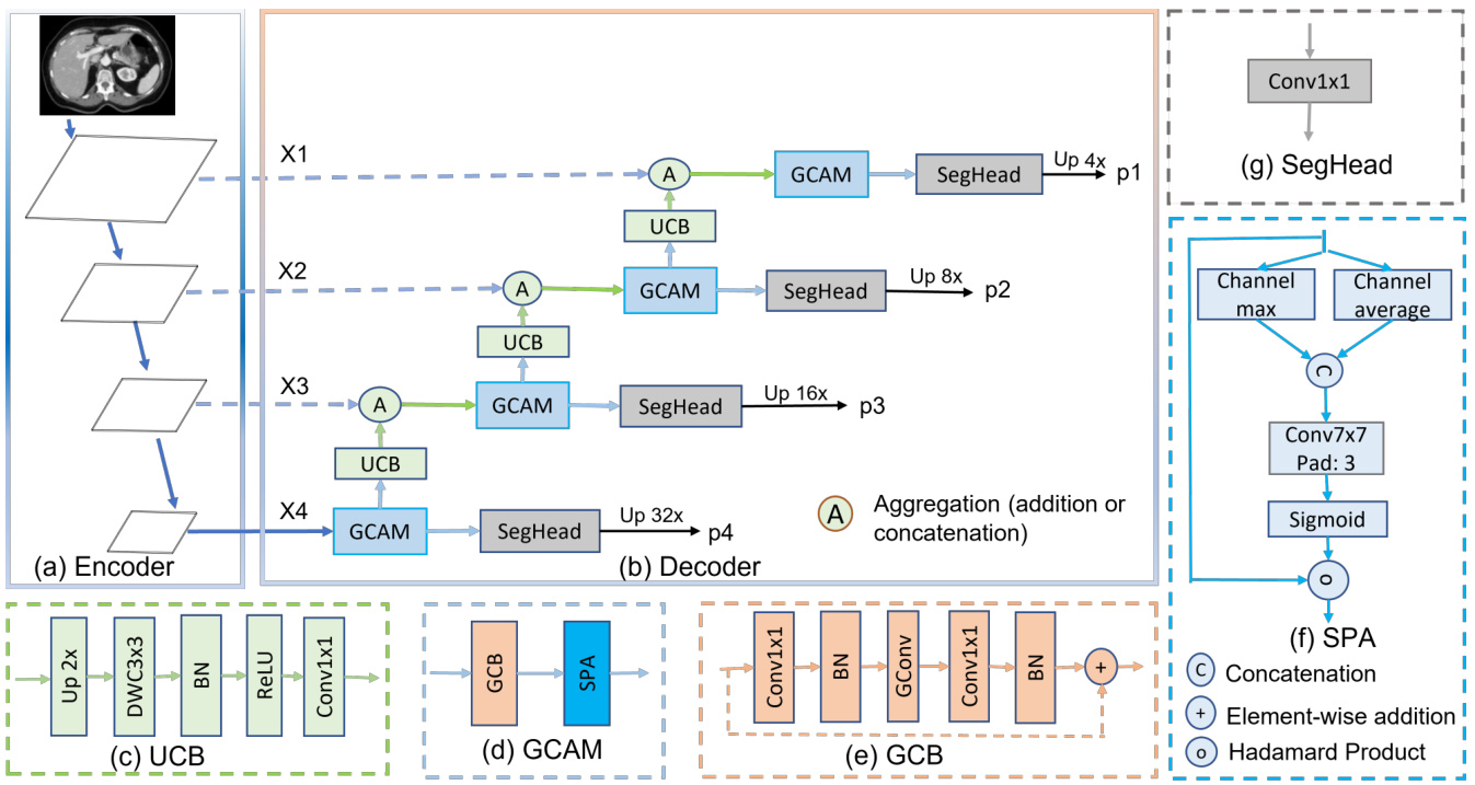
Figure 1. Hierarchical encoder with G-CASCADE network architecture. (a) PVTv2-b2 Encoder backbone with four stages, (b) GCASCADE decoder, (c) Up-convolution block (UCB), (d) Graph convolutional attention module (GCAM), (e) Graph convolution block (GCB), (f) Spatial attention (SPA), and (g) Segmentation head (SegHead). X1, X2, X3, and X4 are the output features of the four stages of hierarchical encoder. p1, p2, p3, and p4 are output segmentation maps from four stages of our decoder.
图 1: 采用 G-CASCADE 网络架构的层次化编码器。(a) 包含四个阶段的 PVTv2-b2 编码器主干,(b) GCASCADE 解码器,(c) 上卷积块 (UCB),(d) 图卷积注意力模块 (GCAM),(e) 图卷积块 (GCB),(f) 空间注意力 (SPA),(g) 分割头 (SegHead)。X1、X2、X3 和 X4 是层次化编码器四个阶段的输出特征。p1、p2、p3 和 p4 是解码器四个阶段输出的分割图。
Attention mechanisms have also been explored in combination with both CNNs [27, 11] and transformer-based archi tec ture s [9] in medical image segmentation. PraNet [11] utilizes the reverse attention mechanism [6]. In PolypPVT [9], authors employ PVTv2 [40] as the encoder and integrates CBAM [43] attention blocks in the decoder, along with other modules. CASCADE [28] proposes a cascaded decoder that utilizes both channel attention [14] and spatial attention [5] modules for feature refinement. CASCADE extracts features from four stages of the transformer encoder and uses cascaded refinement to generate highresolution segmentation maps. Due to incorporating local information with global information of transformers, CASCADE exhibits remarkable performance in medical image segmentation. However, CASCADE decoder has two major limitations: this can lead to i) long-range attention deficit due using only convolution operations during decoding and ii) high computational inefficiency due to using three $3\times3$ convolutions in each stage of the decoder. We propose to use graph convolution to overcome these limitations.
注意力机制在医学图像分割领域已与CNN[27,11]和基于Transformer的架构[9]结合探索。PraNet[11]采用了反向注意力机制[6]。PolypPVT[9]使用PVTv2[40]作为编码器,并在解码器中集成CBAM[43]注意力模块及其他组件。CASCADE[28]提出了一种级联解码器,同时利用通道注意力[14]和空间注意力[5]模块进行特征优化。该方法从Transformer编码器的四个阶段提取特征,通过级联优化生成高分辨率分割图。由于融合了Transformer的局部与全局信息,CASCADE在医学图像分割中表现出色。但该解码器存在两个主要缺陷:i)解码阶段仅使用卷积操作会导致长程注意力缺失;ii)解码器每阶段使用三个$3\times3$卷积导致计算效率低下。我们提出使用图卷积来克服这些局限。
3. Method
3. 方法
In this section, we first introduce a new G-CASCADE decoder, then explain two different transformer-based architectures (i.e., PVT-GCASCADE and MERITGCASCADE) incorporating our proposed decoder.
在本节中,我们首先介绍一种新的 G-CASCADE 解码器,然后阐述两种基于 Transformer 的不同架构 (即 PVT-GCASCADE 和 MERIT-GCASCADE) 如何融入我们提出的解码器。
3.1. Cascaded Graph Convolutional Decoder (GCASCADE)
3.1. 级联图卷积解码器 (GCASCADE)
Existing transformer-based models have limited (local) contextual information processing ability among pixels. As a result, the transformer-based model faces difficulties in locating the more discriminating local features. To address this issue, some works [9, 28, 29] utilize computationally expensive 2D convolution blocks in the decoder. Although the convolution block helps to incorporate the local information, it results in long-range attention deficits. To overcome this problem, we propose a new cascaded graph convolutional decoder, G-CASCADE, for pyramid encoders.
现有基于Transformer的模型在像素间仅具备有限的(局部)上下文信息处理能力,导致这类模型难以定位更具区分度的局部特征。为解决该问题,部分研究[9,28,29]在解码器中采用了计算成本高昂的二维卷积模块。虽然卷积模块有助于整合局部信息,但会导致长程注意力缺失。为此,我们提出了一种面向金字塔编码器的新型级联图卷积解码器G-CASCADE。
As shown in Figure 1(b), G-CASCADE consists of efficient up-convolution blocks (UCBs) to upsample the features, graph convolutional attention modules (GCAMs) to robustly enhance the feature maps, and segmentation heads (SegHeads) to get the segmentation output. We have four GCAMs for the four stages of pyramid features from the encoder. To aggregate the multi-scale features, we first aggregate (e.g., addition or concatenation) the upsampled features from the previous decoder block with the features from the skip connections. Afterward, we process the concatenated features using our GCAM for enhancing semantic information. We then send the output from each GCAM to a prediction head. Finally, we aggregate four different prediction maps to produce the final segmentation output.
如图 1(b) 所示,G-CASCADE 由高效上卷积块 (UCB) 用于特征上采样、图卷积注意力模块 (GCAM) 用于鲁棒增强特征图,以及分割头 (SegHead) 用于生成分割输出。我们对编码器金字塔特征的四个阶段分别配置了四个 GCAM。为聚合多尺度特征,我们首先将前一解码器块的上采样特征与跳跃连接特征进行聚合 (如相加或拼接)。随后使用 GCAM 处理拼接后的特征以增强语义信息。每个 GCAM 的输出会被送入预测头,最终聚合四个不同预测图以生成最终分割输出。
3.1.1 Graph convolutional attention module (GCAM) 3.1.3 Segmentation head (SegHead)
3.1.1 图卷积注意力模块 (GCAM)
3.1.3 分割头 (SegHead)
We use the graph convolutional attention modules to refine the feature maps. GCAM consists of a graph convolution block $(G C B(.))$ to refine the features preserving long-range attention and a spatial attention [5] $(S P A(\cdot))$ block to capture the local contextual information as in Equation 1:
我们使用图卷积注意力模块来优化特征图。GCAM由两部分组成:一个图卷积块 $(G C B(.))$ 用于保持长距离注意力优化特征,以及一个空间注意力 [5] $(S P A(\cdot))$ 块用于捕获局部上下文信息,如公式1所示:
$$
G C A M(x)=S P A(G C B(x))
$$
$$
G C A M(x)=S P A(G C B(x))
$$
where $x$ is the input tensor and $G C A M(\cdot)$ represents the convolutional attention module. Due to using graph convolution, our GCAM is significantly more efficient than the convolutional attention module (CAM) proposed in [28].
其中 $x$ 是输入张量,$G C A M(\cdot)$ 表示卷积注意力模块。由于使用了图卷积,我们的GCAM比[28]中提出的卷积注意力模块(CAM)效率显著更高。
Graph Convolution Block (GCB): The GCB is used to enhance the features generated using our cascaded expanding path. In our GCB, we follow the Grapher design of Vision GNN [13]. GCB consists of a graph convolution layer $G C o n v(.)$ and two $1\times1$ convolution layers $C(\cdot)$ each followed by a batch normalization layer $B N(\cdot)$ and a ReLU activation layer $R(.).G C B(\cdot)$ is formulated as Equation 2:
图卷积块 (GCB): GCB用于增强通过级联扩展路径生成的特征。在我们的GCB中,我们遵循Vision GNN [13]的Grapher设计。GCB由一个图卷积层$G C o n v(.)$和两个$1\times1$卷积层$C(\cdot)$组成,每个卷积层后接批量归一化层$B N(\cdot)$和ReLU激活层$R(.)$。$G C B(\cdot)$的表达式如公式2所示:
$$
G C B(x)=R(B N(C(G C o n v(R(B N(C(x))))))
$$
$$
G C B(x)=R(B N(C(G C o n v(R(B N(C(x))))))
$$
where GConv can be formulated using Equation 3:
GConv 可以用公式 3 表示:
$$
G C o n v(x)=G E L U(B N(D y n C o n v(x)))
$$
$$
G C o n v(x)=G E L U(B N(D y n C o n v(x)))
$$
where DynConv(.) is a graph convolution (e.g., maxrelative, edge, GraphSAGE, and GIN) in dense dilated Knearest neighbour (KNN) graph. $B N(.)$ and $G E L U(.)$ are batch normalization and GELU activation, respectively.
其中DynConv(.)是密集扩张K近邻(KNN)图中的图卷积(例如maxrelative、edge、GraphSAGE和GIN)。$B N(.)$和$G E L U(.)$分别是批归一化和GELU激活函数。
SPatial Attention (SPA): The SPA determines where to focus in a feature map; then it enhances those features. The spatial attention is formulated as Equation 4:
空间注意力 (SPA): SPA决定在特征图中关注哪些位置,然后增强这些特征。空间注意力的计算公式如式4所示:
$$
S P A(x)=S i g m o i d(C o n v([C_{m a x}(x),C_{a v g}(x)]))\circledast x
$$
$$
S P A(x)=S i g m o i d(C o n v([C_{m a x}(x),C_{a v g}(x)]))\circledast x
$$
where Sigmoid(·) is a Sigmoid activation function. $C_{m a x}(\cdot)$ and $C_{a v g}(\cdot)$ represent the maximum and average values obtained along the channel dimension, respectively. $C o n v(\cdot)$ is a $7\times7$ convolution layer with padding 3 to enhance local contextual information (as in [9]). $\circledast$ is the Hadamard product.
其中 Sigmoid(·) 是 Sigmoid 激活函数。$C_{max}(\cdot)$ 和 $C_{avg}(\cdot)$ 分别表示沿通道维度获取的最大值和平均值。$Conv(\cdot)$ 是一个填充为 3 的 $7\times7$ 卷积层 (如 [9] 所述) ,用于增强局部上下文信息。$\circledast$ 表示哈达玛积 (Hadamard product) 。
3.1.2 Up-convolution block (UCB)
3.1.2 上卷积块 (UCB)
UCB progressively upsamples the features of the current layer to match the dimension to the next skip connection. Each UCB layer consists of an UpSampling $U p(\cdot)$ with scale-factor 2, a $3\times3$ depth-wise convolution $D W C(\cdot)$ with groups equal input channels, a batch normalization $B N(\cdot)$ , a $R e L U(.)$ activation, and a $1\times1$ convolution $C o n v(.)$ . The $U C B(\cdot)$ can be formulated as Equation 5:
UCB逐步对当前层的特征进行上采样,以匹配下一跳跃连接的维度。每个UCB层包含一个缩放因子为2的上采样$Up(\cdot)$、一个分组数等于输入通道数的$3\times3$深度卷积$DWC(\cdot)$、一个批量归一化$BN(\cdot)$、一个$ReLU(.)$激活函数以及一个$1\times1$卷积$Conv(.)$。$UCB(\cdot)$可表示为公式5:
$$
U C B(x)=C o n v(R e L U(B N(D W C(U p(x)))))
$$
$$
U C B(x)=C o n v(R e L U(B N(D W C(U p(x)))))
$$
Our UCB is light-weight as we replace the $3\times3$ convolution with a depth-wise convolution after upsampling.
我们的UCB设计轻量,因为在上采样后我们将$3\times3$卷积替换为深度可分离卷积。
SegHead takes refined feature maps from the four stages of the decoder as input and predicts four output segmentation maps. Each SegHead layer consists of a $1\times1$ convolution $C o n v_{1\times1}(\cdot)$ which takes feature maps having $N_{i}$ channels ( $N_{i}$ is the number of channels in the feature map of stage $i\rrangle$ ) as input and gives output with channels equal to number of target classes for multi-class but 1 channel for binary prediction. The $S e g H e a d(\cdot)$ is formulated as Equation 6:
SegHead 以解码器四个阶段的精炼特征图作为输入,并预测四个输出分割图。每个 SegHead 层包含一个 $1\times1$ 卷积 $C o n v_{1\times1}(\cdot)$ ,该卷积以具有 $N_{i}$ 个通道的特征图( $N_{i}$ 是阶段 $i\rrangle$ 特征图的通道数)作为输入,输出通道数等于多分类的目标类别数,但二分类预测时仅输出1个通道。 $S e g H e a d(\cdot)$ 的公式如式6所示:
$$
S e g H e a d(x)=C o n v_{1\times1}(x)
$$
$$
S e g H e a d(x)=C o n v_{1\times1}(x)
$$
3.2. Overall architecture
3.2. 整体架构
To ensure effective generalization and the ability to process multi-scale features in medical image segmentation, we integrate our proposed G-CASCADE decoder with two different hierarchical backbone encoder networks such as PVTv2 [40] and MERIT [29]. PVTv2 utilizes convolution operations instead of traditional transformer patch embedding modules to consistently capture spatial information. MERIT utilizes two MaxViT [34] encoders with varying window sizes for self-attention, thus enabling the capture of multi-scale features.
为确保医学图像分割中有效的泛化能力和多尺度特征处理能力,我们将提出的G-CASCADE解码器与两种不同的分层主干编码器网络(如PVTv2 [40]和MERIT [29])相结合。PVTv2采用卷积运算替代传统的Transformer块嵌入模块,以持续捕获空间信息。MERIT利用两个具有不同窗口大小的MaxViT [34]编码器进行自注意力计算,从而能够捕获多尺度特征。
By utilizing the PVTv2-b2 (Standard) encoder, we create the PVT-GCASCADE architecture. To adopt PVTv2- b2, we first extract the features (X1, X2, X3, and X4) from four layers and feed them (i.e., X4 in the upsample path and X3, X2, X1 in the skip connections) into our G-CASCADE decoder as shown in Figure 1(a-b). Then, the G-CASCADE processes them and produces four prediction maps that correspond to the four stages of the encoder network.
通过采用PVTv2-b2(标准)编码器,我们构建了PVT-GCASCADE架构。在适配PVTv2-b2时,首先从四个层级提取特征(X1、X2、X3和X4),并将它们(即上采样路径中的X4和跳跃连接中的X3、X2、X1)输入到我们的G-CASCADE解码器中,如图1(a-b)所示。随后,G-CASCADE处理这些特征并生成四个预测图,分别对应编码器网络的四个阶段。
Besides, we introduce the new MERIT-GCASCADE architecture by adopting the architectural design of the MERIT network. In the case of MERIT, we only replace their decoder with our proposed decoder and keep their hybrid CNN-transformer MaxViT [34] encoder networks. In our MERIT-GCASCADE architecture, we extract hierarchical feature maps from four stages of first encoder and then feed them to the corresponding decoder. Afterwards, we aggregate the feedback from final stage of the decoder to the input image and feed them to second encoder having different window sizes for self-attention. We extract feature maps from four stages of the second decoder and feed them to the second decoder. We send cascaded skip connections like MERIT [29] to the second decoder. We get four output segmentation maps from the four stages of our second decoder. Finally, we aggregate the segmentation maps from the two decoders for four stages separately to produce four output segmentation maps. Our proposed decoder is designed to be adaptable and seamlessly integrates with other hierarchical backbone networks.
此外,我们通过采用MERIT网络架构设计,引入了新型MERIT-GCASCADE架构。对于MERIT部分,我们仅将其解码器替换为我们提出的解码器,同时保留其混合CNN-Transformer MaxViT [34]编码器网络。在MERIT-GCASCADE架构中,我们首先从第一编码器的四个阶段提取分层特征图,并将其输入对应解码器。随后,我们将解码器最终阶段的反馈与输入图像聚合,并馈送至具有不同自注意力窗口大小的第二编码器。从第二编码器的四个阶段提取特征图后输入第二解码器,同时像MERIT [29]那样向第二解码器发送级联跳跃连接。第二解码器的四个阶段会生成四张输出分割图,最终我们将两个解码器四个阶段的分割图分别聚合,独立生成四张输出分割图。所提出的解码器具备适配性,可与其他分层主干网络无缝集成。
3.3. Multi-stage outputs and loss aggregation
3.3. 多阶段输出与损失聚合
We get four output segmentation maps $p_{1},p_{2},p_{3}$ , and $p_{4}$ from the four prediction heads for the four stages of our G-CASCADE decoder.
我们得到四个输出分割图 $p_{1},p_{2},p_{3}$ 和 $p_{4}$,分别来自G-CASCADE解码器四个阶段的预测头。
Output segmentation maps aggregation: We compute the final segmentation output using additive aggregation as in Equation 7:
输出分割图聚合:我们使用如公式7所示的加法聚合计算最终分割输出:
$$
s e g_o u t p u t=\alpha p_{1}+\beta p_{2}+\gamma p_{3}+\zeta p_{4}
$$
$$
s e g_o u t p u t=\alpha p_{1}+\beta p_{2}+\gamma p_{3}+\zeta p_{4}
$$
where $\alpha, \beta,~\gamma$ , and $\zeta$ are the weights of each prediction head. We set $\alpha,\beta,\gamma$ , and $\zeta$ to 1.0 in all our experiments. We get the final prediction output by applying the Sigmoid activation for binary segmentation and Softmax activation for multi-class segmentation.
其中 $\alpha, \beta,~\gamma$ 和 $\zeta$ 是每个预测头的权重。在所有实验中,我们将 $\alpha,\beta,\gamma$ 和 $\zeta$ 设为1.0。通过应用Sigmoid激活函数进行二值分割,Softmax激活函数进行多类分割,得到最终的预测输出。
Loss aggregation: Following MERIT [29], we use the combinatorial loss aggregation strategy, MUTATION in all our experiments. Therefore, we compute the loss for $2^{n}-1$ comb in a tro rial predictions synthesized from $n$ heads separately and then do a summation of them. We optimize this additive combinatorial loss during training.
损失聚合:遵循MERIT [29],我们在所有实验中使用组合损失聚合策略MUTATION。因此,我们分别计算由$n$个头合成的$2^{n}-1$种组合的损失,然后对它们求和。在训练过程中,我们优化这个加法组合损失。
4. Experimental Evaluation
4. 实验评估
In this section, we first describe the dataset and evaluation metrics followed by implementation details. Then, we conduct a comparative analysis between our proposed GCASCADE decoder-based architectures and SOTA methods to highlight the superior performance of our approach.
在本节中,我们首先描述数据集和评估指标,随后介绍实现细节。接着,通过对比分析我们提出的基于GCASCADE解码器的架构与SOTA方法,以突显本方案的优越性能。
4.1. Datasets
4.1. 数据集
We present the description of Synapse Multi-organ and ACDC datasets below. The description of ISIC2018, polyp, and retinal vessels segmentation datasets are available in supplementary materials (Section A).
我们在下文介绍Synapse多器官和ACDC数据集的描述。ISIC2018、息肉和视网膜血管分割数据集的描述可在补充材料(A节)中找到。
Synapse Multi-organ dataset. The Synapse Multiorgan dataset1 contains 30 abdominal CT scans which have 3779 axial contrast-enhanced slices. Each CT scan has 85- 198 slices of $512\times512$ pixels. Similar to TransUNet [4], we divide the dataset randomly into 18 scans for training (2212 axial slices) and 12 scans for validation. We segment only 8 abdominal organs, i.e., aorta, gallbladder (GB), left kidney (KL), right kidney (KR), liver, pancreas (PC), spleen (SP), and stomach (SM).
Synapse多器官数据集。Synapse多器官数据集1包含30个腹部CT扫描,共计3779张轴向对比增强切片。每个CT扫描有85-198张切片,分辨率为$512\times512$像素。与TransUNet [4]类似,我们将数据集随机划分为18个扫描用于训练(2212张轴向切片)和12个扫描用于验证。我们仅分割8个腹部器官,即主动脉、胆囊(GB)、左肾(KL)、右肾(KR)、肝脏、胰腺(PC)、脾脏(SP)和胃(SM)。
ACDC dataset. The ACDC dataset2 contains 100 cardiac MRI scans each of which consists of three organs, right ventricle (RV), myocardium (Myo), and left ventricle (LV). Following TransUNet [4], we use 70 cases (1930 axial slices) for training, 10 for validation, and 20 for testing.
ACDC数据集。ACDC数据集包含100例心脏MRI扫描,每例包含三个器官:右心室 (RV)、心肌 (Myo) 和左心室 (LV)。按照TransUNet [4]的设置,我们使用70例 (1930个轴向切片) 进行训练,10例用于验证,20例用于测试。
4.2. Evaluation metrics
4.2. 评估指标
We use DICE, mIoU, and $95%$ Hausdorff Distance (HD95) to evaluate performance on the Synapse Multiorgan dataset. However, for the ACDC dataset, we use only DICE score as an evaluation metrics. We use DICE and mIoU as the evaluation metrics in polyp segmentation and ISIC2018 datasets. The DICE score $\bar{D}S\bar{C}(Y,\hat{Y})$ , $I o U(Y,{\hat{Y}})$ , and HD95 distance $D_{H}(Y,{\hat{Y}})$ are calculated using Equations 8, 9, and 10, respectively.
我们使用DICE、mIoU和$95%$豪斯多夫距离(HD95)来评估Synapse多器官数据集的性能。而对于ACDC数据集,我们仅采用DICE分数作为评估指标。在息肉分割和ISIC2018数据集中,我们使用DICE和mIoU作为评估指标。DICE分数$\bar{D}S\bar{C}(Y,\hat{Y})$、$I o U(Y,{\hat{Y}})$以及HD95距离$D_{H}(Y,{\hat{Y}})$分别通过公式8、9和10计算得出。
$$
D S C(Y,{\hat{Y}})={\frac{2\times|Y\cap{\hat{Y}}|}{|Y|+|{\hat{Y}}|}}\times100\quad
$$
$$
D S C(Y,{\hat{Y}})={\frac{2\times|Y\cap{\hat{Y}}|}{|Y|+|{\hat{Y}}|}}\times100\quad
$$
$$
I o U(Y,\hat{Y})=\frac{|Y\cap\hat{Y}|}{|Y\cup\hat{Y}|}\times100
$$
$$
I o U(Y,\hat{Y})=\frac{|Y\cap\hat{Y}|}{|Y\cup\hat{Y}|}\times100
$$
$$
D_{H}(Y,\hat{Y})=\operatorname*{max}{\operatorname*{max}{y\in Y}\operatorname*{min}{\hat{y}\in\hat{Y}}d(y,\hat{y}),{\operatorname*{max}{\hat{y}\in\hat{Y}}\operatorname*{min}_{y\in Y}d(y,\hat{y})}
$$
$$
D_{H}(Y,\hat{Y})=\operatorname*{max}{\operatorname*{max}{y\in Y}\operatorname*{min}{\hat{y}\in\hat{Y}}d(y,\hat{y}),{\operatorname*{max}{\hat{y}\in\hat{Y}}\operatorname*{min}_{y\in Y}d(y,\hat{y})}
$$
where $Y$ and $\hat{Y}$ are the ground truth and predicted segmentation map, respectively.
其中 $Y$ 和 $\hat{Y}$ 分别表示真实分割图和预测分割图。
4.3. Implementation details
4.3. 实现细节
We use Pytorch 1.11.0 to implement our network and conduct experiments. We train all models on a single NVIDIA RTX A6000 GPU with 48GB of memory. We use the PVTv2-b2 and Small Cascaded MERIT as representative network. We use the pre-trained weights on ImageNet for both PVT and MERIT backbone networks. We train our model using AdamW optimizer [24] with both learning rate and weight decay of 0.0001.
我们使用 PyTorch 1.11.0 实现网络并进行实验。所有模型均在单块 NVIDIA RTX A6000 GPU (48GB显存) 上训练,选用 PVTv2-b2 和 Small Cascaded MERIT 作为代表性网络架构。PVT 和 MERIT 主干网络均加载 ImageNet 预训练权重,采用 AdamW 优化器 [24] 进行训练,学习率和权重衰减率均设为 0.0001。
GCB: We construct dense dilated graph using $K=11$ neighbors for KNN and use the Max-Relative (MR) graph convolution in all our experiments. The batch normalization is used after MR graph convolution. Following ViG [13], we also use the relative position vector for graph construction and reduction ratios of [1, 1, 4, 2] for graph convolution block in different stages.
GCB:我们使用$K=11$个邻居构建密集扩张图进行KNN,并在所有实验中采用最大相对 (MR) 图卷积。MR图卷积后应用批量归一化。遵循ViG [13],我们同样采用相对位置向量进行图构建,并在不同阶段的图卷积块中使用[1, 1, 4, 2]的缩减比例。
Synapse Multi-organ dataset. We use a batch size of 6 and train each model for maximum of 300 epochs. We use the input resolution of $224\times224$ for PVT-GCASCADE and $256\times256$ , $224\times224;$ ) for MERIT-GCASCADE. We apply random rotation and flipping for data augmentation. The combined weighted Cross-entropy (0.3) and DICE (0.7) loss are utilized as the loss function.
Synapse 多器官数据集。我们使用批大小为6,每个模型最多训练300个周期。PVT-GCASCADE的输入分辨率为$224\times224$,MERIT-GCASCADE的输入分辨率为$256\times256$和$224\times224$。我们采用随机旋转和翻转进行数据增强。损失函数采用加权交叉熵(0.3)和DICE(0.7)的组合损失。
ACDC dataset. For the ACDC dataset, we train each model for a maximum of 150 epochs with a batch size of 12. We set the input resolution as $224\times224$ for PVTGCASCADE and $(256~\times 256~\$ , $224\times224_{,}$ ) for MERITGCASCADE. We apply random flipping and rotation for data augmentation. We optimize the combined weighted Cross-entropy (0.3) and DICE (0.7) loss function.
ACDC数据集。对于ACDC数据集,我们将每个模型的最大训练周期设为150,批量大小为12。PVTGCASCADE的输入分辨率设置为$224\times224$,MERITGCASCADE则为$(256~\times 256~\$ , $224\times224_{,}$)。数据增强采用随机翻转和旋转。优化目标为加权交叉熵(0.3)与DICE(0.7)的组合损失函数。
Table 1. Results of Synapse Multi-organ segmentation. We report only DICE scores for individual organs. We get the results of UNet, AttnUNet, PolypPVT, S S Former PV T, TransUNet, and SwinUNet from [28]. We reproduce the results of Cascaded MERIT with a batch size of 6. $\uparrow(\downarrow)$ denotes the higher (lower) the better. G-CASCADE results are averaged over five runs. The best results are shown in bold.
表 1: Synapse多器官分割结果。我们仅报告各器官的DICE分数。UNet、AttnUNet、PolypPVT、SSFormerPVT、TransUNet和SwinUNet的结果来自[28]。我们使用批量大小为6复现了Cascaded MERIT的结果。$\uparrow(\downarrow)$表示越高(低)越好。G-CASCADE结果为五次运行的平均值,最佳结果以粗体显示。
| 架构 | DICE↑ | HD95↓ | mloU↑ | 主动脉 | 胆囊 | 左肾 | 右肾 | 肝脏 | 胰腺 | 脾脏 | 胃 |
|---|---|---|---|---|---|---|---|---|---|---|---|
| UNet [30] | 70.11 | 44.69 | 59.39 | 84.00 | 56.70 | 72.41 | 62.64 | 86.98 | 48.73 | 81.48 | 67.96 |
| AttnUNet [27] | 71.70 | 34.47 | 61.38 | 82.61 | 61.94 | 76.07 | 70.42 | 87.54 | 46.70 | 80.67 | 67.66 |
| R50+UNet [4] | 74.68 | 36.87 | - | 84.18 | 62.84 | 79.19 | 71.29 | 93.35 | 48.23 | 84.41 | 73.92 |
| R50+AttnUNet [4] | 75.57 | 36.97 | - | 55.92 | 63.91 | 79.20 | 72.71 | 93.56 | 49.37 | 87.19 | 74.95 |
| SSFormerPVT[38] | 78.01 | 25.72 | 67.23 | 82.78 | 63.74 | 80.72 | 78.11 | 93.53 | 61.53 | 87.07 | 76.61 |
| PolypPVT [9] | 78.08 | 25.61 | 67.43 | 82.34 | 66.14 | 81.21 | 73.78 | 94.37 | 59.34 | 88.05 | 79.40 |
| TransUNet [4] | 77.61 | 26.90 | 67.32 | 86.56 | 60.43 | 80.54 | 78.53 | 94.33 | 58.47 | 87.06 | 75.00 |
| SwinUNet [2] | 77.58 | 27.32 | 66.88 | 81.76 | 65.95 | 82.32 | 79.22 | 93.73 | 53.81 | 88.04 | 75.79 |
| MT-UNet [37] | 78.59 | 26.59 | - | 87.92 | 64.99 | 81.47 | 77.29 | 93.06 | 59.46 | 87.75 | 76.81 |
| MISSFormer [16] | 81.96 | 18.20 | - | 86.99 | 68.65 | 85.21 | 82.00 | 94.41 | 65.67 | 91.92 | 80.81 |
| PVT-CASCADE [28] | 81.06 | 20.23 | 70.88 | 83.01 | 70.59 | 82.23 | 80.37 | 94.08 | 64.43 | 90.10 | 83.69 |
| TransCASCADE [28] | 82.68 | 17.34 | 73.48 | 86.63 | 68.48 | 87.66 | 84.56 | 94.43 | 65.33 | 90.79 | 83.52 |
| Cascaded MERIT [29] | 84.32 | 14.27 | 75.44 | 86.67 | 72.63 | 87.71 | 84.62 | 95.02 | 70.74 | 91.98 | 85.17 |
| PVT-GCASCADE (Ours) | 83.28 | 15.83 | 73.91 | 86.50 | 71.71 | 87.07 | 83.77 | 95.31 | 66.72 | 90.84 | 83.58 |
| MERIT-GCASCADE (Ours) | 84.54 | 10.38 | 75.83 | 88.05 | 74.81 | 88.01 | 84.83 | 95.38 | 69.73 | 91.92 | 83.63 |
Table 2. Results on ACDC dataset. DICE scores are reported for individual organs. We get the results of SwinUNet from [28]. GCASCADE results are averaged over five runs. The best results are shown in bold.
表 2: ACDC数据集上的结果。DICE分数针对各个器官进行报告。我们从[28]中获取了SwinUNet的结果。GCASCADE结果是五次运行的平均值。最佳结果以粗体显示。
| 方法 | 平均 | Dice | RV | Myo | LV |
|---|---|---|---|---|---|
| R50+UNet[4] | 87.55 | 87.10 | 80.63 | 94.92 | |
| R50+AttnUNet[4] | 86.75 | 87.58 | 79.20 | 93.47 | |
| ViT+CUP [4] | 81.45 | 81.46 | 70.71 | 92.18 | |
| R50+ViT+CUP [4] | 87.57 | 86.07 | 81.88 | 94.75 | |
| TransUNet [4] | 89.71 | 86.67 | 87.27 | 95.18 | |
| SwinUNet [2] | 88.07 | 85.77 | 84.42 | 94.03 | |
| MT-UNet [37] | 90.43 | 86.64 | 89.04 | 95.62 | |
| MISSFormer [16] | 90.86 | 89.55 | 88.04 | 94.99 | |
| PVT-CASCADE[28] | 91.46 | 89.97 | 88.9 | 95.50 | |
| TransCASCADE [28] | 91.63 | 90.25 | 89.14 | 95.50 | |
| Cascaded MERIT [29] | 91.85 | 90.23 | 89.53 | 95.80 | |
| PVT-GCASCADE (Ours) | 91.95 | 90.31 | 89.63 | 95.91 | |
| MERIT-GCASCADE (Ours) | 92.23 | 90.64 | 89.96 | 96.08 |
ISIC2018 dataset: We resize the images into $384\times384$ resolution. Then, we train our model for 200 epochs with a batch size of 4 and a gradient clip of 0.5. We optimize the combined weighted BCE and weighted IoU loss function.
ISIC2018数据集:我们将图像尺寸调整为$384\times384$分辨率,随后以批量大小4和梯度裁剪值0.5训练模型200个周期,并优化加权BCE与加权IoU的混合损失函数。
Polyp datasets. We resize the image to $352\times352$ and use a multi-scale ${0.75,1.0,1.25}$ training strategy with a gradient clip limit of 0.5 like CASCADE [28]. We use a batch size of 4 and train each model a maximum of 200 epochs. We optimize the combined weighted BCE and weighted IoU loss function.
息肉数据集。我们将图像大小调整为$352\times352$,并采用类似CASCADE [28]的多尺度${0.75,1.0,1.25}$训练策略,梯度裁剪限制为0.5。使用批量大小为4,每个模型最多训练200个周期。我们优化了加权BCE和加权IoU的组合损失函数。
4.4. Results
4.4. 结果
We compare our architectures (i.e., PVT-GCASCADE and MERIT-GCASCADE) with SOTA CNN and transformer-based segmentation methods on Synapse Multi-organ, ACDC, ISIC2018 [8], and Polyp (i.e., Endoscene [35], CVC-ClinicDB [1], Kvasir [18], ColonDB [32]) datasets. The results of ISIC2018, polyp, and retinal vessels segmentation datasets are reported in the supplementary materials (Section B).
我们在Synapse多器官、ACDC、ISIC2018 [8] 以及息肉 (即Endoscene [35]、CVC-ClinicDB [1]、Kvasir [18]、ColonDB [32]) 数据集上,将我们的架构 (即PVT-GCASCADE和MERIT-GCASCADE) 与基于CNN和Transformer的最先进 (SOTA) 分割方法进行了对比。ISIC2018、息肉及视网膜血管分割数据集的结果详见补充材料 (B部分)。
4.4.1 Quantitative results on Synapse Multi-organ dataset
4.4.1 Synapse多器官数据集的定量结果
Table 1 presents the performance of different CNNand transformer-based methods on Synapse Multi-organ segmentation dataset. We can see from Table 1 that our MERIT-GCASCADE significantly outperforms all the SOTA CNN- and transformer-based 2D medical image segmentation methods thus achieving the best average DICE score of $84.54%$ . Our PVT-GCASCADE and MERIT-GCASCADE outperforms their counterparts PVTCASCADE and Cascaded MERIT by $2.22%$ and $0.22%$ DICE scores, respectively with significantly lower computational costs. Similarly, our PVT-GCASCADE and MERIT-GCASCADE outperforms their counterparts by 4.4 and 3.89 in HD95 distance. Our MERIT-GCASCADE has the lowest HD95 distance (10.38) which is 3.89 lower than the best SOTA method Cascaded MERIT (HD95 of 14.27). The lower HD95 scores indicate that our G-CASCADE decoder can better locate the boundary of organs.
表 1: 不同基于 CNN 和 Transformer 的方法在 Synapse 多器官分割数据集上的性能表现。从表 1 可以看出,我们的 MERIT-GCASCADE 显著优于所有基于 CNN 和 Transformer 的 SOTA 二维医学图像分割方法,从而实现了 84.54% 的最佳平均 DICE 分数。我们的 PVT-GCASCADE 和 MERIT-GCASCADE 分别以 2.22% 和 0.22% 的 DICE 分数优势超越其对应方法 PVTCASCADE 和 Cascaded MERIT,同时计算成本显著降低。同样,在 HD95 距离指标上,我们的 PVT-GCASCADE 和 MERIT-GCASCADE 分别以 4.4 和 3.89 的优势超越对应方法。我们的 MERIT-GCASCADE 取得了最低的 HD95 距离 (10.38) ,比最佳 SOTA 方法 Cascaded MERIT (HD95 为 14.27) 降低了 3.89。更低的 HD95 分数表明我们的 G-CASCADE 解码器能更准确定位器官边界。
Our proposed decoder also shows boost in the DICE scores of individual organ segmentation. We can see from the Table 1 that our proposed MERIT-GCASCADE significantly outperforms SOTA methods on five out of eight organs. We believe that G-CASCADE decoder demonstrates better performance due to using graph convolution together with the transformer encoder.
我们提出的解码器在单个器官分割的DICE分数上也显示出提升。从表1可以看出,我们提出的MERIT-GCASCADE在八个器官中的五个上显著优于SOTA方法。我们认为G-CASCADE解码器由于同时使用了图卷积和Transformer编码器,因此表现出更好的性能。
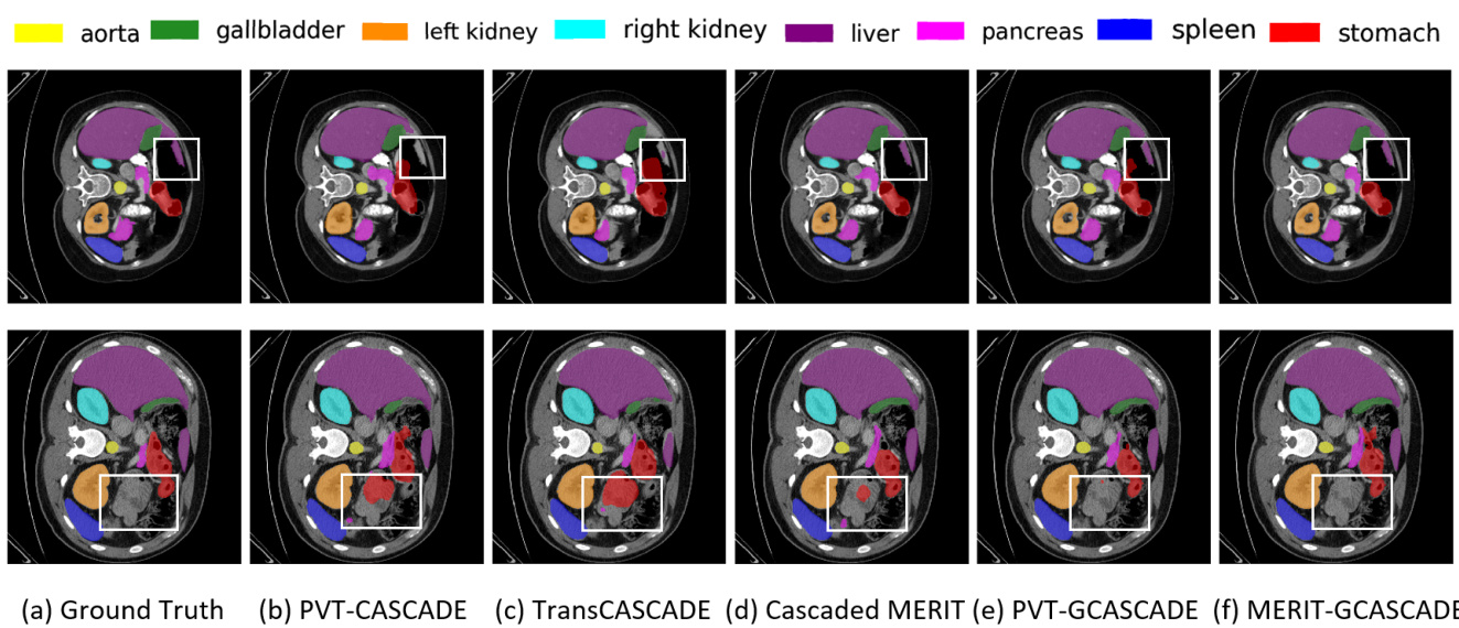
Figure 2. Qualitative results on Synapse multi-organ dataset. (a) Ground Truth (GT), (b) PVT-CASCADE, (c) Trans CASCADE, (d) Cascaded MERIT, (e) PVT-GCASCADE, and (f) MERIT-GCASCADE. We overlay the segmentation maps on top of original image/slice. We use the white bounding box to highlight regions where most of the methods have incorrect predictions.
图 2: Synapse多器官数据集的定性结果。(a) 真实标注 (GT), (b) PVT-CASCADE, (c) Trans CASCADE, (d) Cascaded MERIT, (e) PVT-GCASCADE, (f) MERIT-GCASCADE。我们在原始图像/切片上叠加分割结果图。白色边框标注了多数方法预测错误的区域。
4.4.2 Quantitative results on ACDC dataset
4.4.2 ACDC数据集上的定量结果
We have conducted another set of experiments on the MRI images of the ACDC dataset using our architectures. Table 2 presents the average DICE scores of our PVTGCASCADE and MERIT-GCASCADE along with other SOTA methods. Our MERIT-GCASCADE achieves the highest average DICE score of $92.23%$ thus improving about $0.38%$ over Cascaded MERIT though our decoder has significantly lower computational cost (see Table 5). Our PVT-GCASCADE gains $91.95%$ DICE score which is also better than all other methods. Besides, both our PVTGCASCADE and MERIT-GCASCADE have better DICE scores in all three organs segmentation.
我们在ACDC数据集的MRI图像上使用我们的架构进行了另一组实验。表2展示了我们的PVTGCASCADE和MERIT-GCASCADE以及其他SOTA方法的平均DICE分数。我们的MERIT-GCASCADE实现了最高的平均DICE分数$92.23%$,比Cascaded MERIT提高了约$0.38%$,尽管我们的解码器计算成本显著更低 (见表5)。我们的PVT-GCASCADE获得了$91.95%$的DICE分数,也优于所有其他方法。此外,我们的PVTGCASCADE和MERIT-GCASCADE在所有三个器官分割中都具有更好的DICE分数。
4.4.3 Qualitative results on Synapse Multi-organ dataset
4.4.3 Synapse多器官数据集的定性结果
We present the segmentation outputs of our proposed method and three other SOTA methods on two sample images in Figure 2. If we look into the highlighted regions in both samples, we can see that MERIT-GCASCADE consistently segments the organs with minimal false negative and false positive results. PVT-GCASCADE and Cascaded MERIT show comparable results. PVT-GCASCADE has false positives in first sample (i.e., first row) and has better segmentation in second sample (i.e., second row), whereas Cascaded MERIT provides better segmentation in first sample but it has larger false positives in second sample. TransCASCADE and PVT-CASCADE provide larger incorrect segmentation outputs in both samples.
我们在图2中展示了所提方法及其他三种SOTA方法在两幅样本图像上的分割结果。观察两个样本的高亮区域可见,MERIT-GCASCADE始终能以最少的假阴性和假阳性结果分割器官。PVT-GCASCADE与Cascaded MERIT表现相当:PVT-GCASCADE在第一个样本(即第一行)存在假阳性,但在第二个样本(即第二行)分割效果更好;而Cascaded MERIT在第一个样本分割更优,却在第二个样本出现更多假阳性。TransCASCADE和PVT-CASCADE在两组样本中均产生较多错误分割结果。
Table 3. Quantitative results of different components of GCASCADE with PVTv2-b2 encoder on Synapse multi-organ dataset. We use additive aggregation for adding skip connections and an input resolution of $224\times224$ to get these results. All results are averaged over five runs. The best results are showed in bold.
表 3. 采用PVTv2-b2编码器的GCASCADE各组件在Synapse多器官数据集上的量化结果。我们使用加法聚合进行跳跃连接,输入分辨率为$224\times224$以获得这些结果。所有结果为五次运行的平均值,最佳结果以粗体显示。
| 组件 | SPA | FLOPs (G) | #Params (M) | Avg DICE | |
|---|---|---|---|---|---|
| 级联 | GCB | ||||
| 否 | 否 | 否 | 0 | 0 | 80.1±0.2 |
| 是 | 否 | 否 | 0.102 | 0.225 | 81.1±0.2 |
| 是 | 否 | 是 | 0.102 | 0.225 | 82.1±0.3 |
| 是 | 是 | 否 | 0.341 | 1.78 | 83.0±0.2 |
| 是 | 是 | 是 | 0.342 | 1.78 | 83.3±0.2 |
Table 4. Comparison of different arrangements of GCB and SPA in GCAM on Synapse Multi-organ dataset. We use PVTv2-b2 as the encoder to produce these results. All the results are averaged over five runs. The best results are in bold.
表 4: GCAM中GCB和SPA不同排列方式在Synapse Multi-organ数据集上的对比。我们使用PVTv2-b2作为编码器生成这些结果。所有结果均为五次运行的平均值,最佳结果以粗体显示。
| 排列方式 | DICE (%) |
|---|---|
| SPA→GCB | 82.93±0.2 |
| GCB→→SPA (Ours) | 83.28±0.2 |
Table 5. Comparison with the baseline decoder on Synapse Multiorgan dataset. We only report the FLOPs and the number of parameters of the respective decoder. We produce these results using PVTv2-b2 encoder. All the results are averaged over five runs. The best results are in bold.
表5: 在Synapse多器官数据集上与基线解码器的对比。我们仅报告了各解码器的FLOPs和参数量。这些结果是使用PVTv2-b2编码器生成的。所有结果均为五次运行的平均值。最佳结果以粗体显示。
Table 6. Comparison of different skip-aggregations in GCASCADE decoder on Synapse Multi-organ dataset. We only report the FLOPs and number of parameters of the respective decoder. PVTV2-b2 encoder has 3.91G FLOPS and 24.86M parameters. Small MERIT encoder has 24.62G FLOPs and 129.38M parameters. All the results are averaged over five runs.
表 6: Synapse多器官数据集上GCASCADE解码器中不同跳跃聚合方式的对比。我们仅报告了各解码器的FLOPs和参数量。PVTV2-b2编码器具有3.91G FLOPs和24.86M参数。Small MERIT编码器具有24.62G FLOPs和129.38M参数。所有结果为五次运行的平均值。
| 解码器 | UCB | FLOPs(G) | #Params(M) | DICE (%) |
|---|---|---|---|---|
| CASCADE | Original | 1.93 | 9.27 | 82.78 |
| CASCADE | Modified | 1.22 | 7.58 | 82.79 |
| G-CASCADE (Ours) | Original | 1.06 | 3.47 | 83.15 |
| G-CASCADE (Ours) | Modified | 0.342 | 1.78 | 83.28 |
| 架构 (Architectures) | 聚合方式 (Aggregation) | 计算量 (FLOPs, G) | 参数量 (#Params, M) | DICE(%) |
|---|---|---|---|---|
| PVT-GCASCADE | 加法 (Addition) | 0.342 | 1.78 | 83.28 |
| PVT-GCASCADE | 拼接 (Concat) | 0.975 | 3.32 | 83.40 |
| MERIT-GCASCADE | 加法 (Addition) | 1.523 | 3.55 | 84.54 |
| MERIT-GCASCADE | 拼接 (Concat) | 4.27 | 5.99 | 84.63 |
5. Ablation Study
5. 消融实验
In this section, we perform a set of ablation experiments that aim to address various questions concerning our proposed architectures and experimental setup. More ablation studies are available in supplementary materials (Section C).
在本节中,我们进行了一系列消融实验,旨在解决关于我们提出的架构和实验设置的各种问题。更多消融研究可在补充材料(C节)中找到。
5.1. Effect of different components of G-CASCADE
5.1. G-CASCADE不同组件的影响
We carry out ablation studies on the Synapse Multiorgan dataset to evaluate the effectiveness of different components of our proposed G-CASCADE decoder. We use the same PVTv2-b2 backbone pre-trained on ImageNet and the same experimental settings for Synapse Multi-organ dataset in all experiments. We remove different modules such as Cascaded structure, GCB, and SPA from the G-CASCADE decoder and compare the results. It is evident from Table 3 that the cascaded structure of the decoder improves performance over the non-cascaded decoder. GCB and SPA modules also help improve performance. However, the use of both SPA and GCB modules together produces the best DICE score of $83.3%$ . We can also see from the table that DICE score is improved about $3.2%$ with 0.342G and 1.78M additional FLOPs and parameters, respectively.
我们在Synapse多器官数据集上进行消融实验,以评估所提出的G-CASCADE解码器中不同组件的有效性。所有实验均使用ImageNet预训练的相同PVTv2-b2主干网络及相同的Synapse多器官数据集实验设置。我们依次移除解码器中的级联结构(Cascaded)、GCB和SPA模块并进行结果对比。表3清晰显示:解码器的级联结构相比非级联版本能提升性能,GCB和SPA模块也分别带来增益。当同时使用SPA和GCB模块时,可获得83.3%的最佳DICE分数。表中数据表明,在额外增加0.342G FLOPs和1.78M参数的情况下,DICE分数提升了约3.2%。
5.2. Effect of arrangements of GCB and SPA in GCAM
5.2. GCAM中GCB和SPA排列方式的影响
We have conducted an ablation study to see the effect of the order of GCB and SPA in GCAM. Table 4 presents the experimental results of two different arrangements. We can conclude from Table 4 that GCB followed by SPA block performs better than SPA followed by GCB. Therefore, in our G-CASCADE decoder, we use a GCB followed by a SPA block in each GCAM.
我们进行了消融实验以研究GCAM中GCB和SPA顺序的影响。表4展示了两种不同排列的实验结果。从表4可以得出结论,先GCB后SPA块的性能优于先SPA后GCB。因此,在我们的G-CASCADE解码器中,每个GCAM都采用先GCB后SPA块的结构。
5.3. Comparison with the baseline decoder
5.3. 与基线解码器的对比
Table 5 reports the experimental results with the computational complexity of our baseline CASCADE decoder and our proposed G-CASCADE decoder. We also report the results of original UpConv used in the CASCADE decoder and our modified efficient UCB. From Table 5, we can see that our modified UCB performs equal or better with significantly lower FLOPs and parameters. Our G-CASCADE decoder provides $0.5%$ better DICE score than the CASCADE decoder with $80.8%$ fewer parameters and $82.3%$ fewer FLOPs.
表 5 报告了我们的基线 CASCADE 解码器和提出的 G-CASCADE 解码器在计算复杂度方面的实验结果。我们还报告了 CASCADE 解码器中使用的原始 UpConv 以及我们改进的高效 UCB 的结果。从表 5 可以看出,改进后的 UCB 在显著降低 FLOPs 和参数量的情况下,性能相当或更好。我们的 G-CASCADE 解码器比 CASCADE 解码器提供了 $0.5%$ 更高的 DICE 分数,同时参数减少了 $80.8%$,FLOPs 减少了 $82.3%$。
5.4. Effect of different skip-aggregations in GCASCADE decoder
5.4. GCASCADE解码器中不同跳跃聚合方式的影响
We conduct some experiments to see the effect of Additive or Concatenation in aggregating upsampled features with the skip-connections. Table 6 presents the results of PVT-GCASCADE and MERIT-GCASCADE with Additive and concatenation aggregations. We can see from Table 6 that Concatenation-based aggregation achieves marginally better DICE scores than Additive aggregation, while having significantly higher FLOPs and parameters. The reason behind this increase in computational complexity is the use of GCAM with the concatenated channels (i.e., $2\times$ of original channels). Considering the lower computational complexity of Additive aggregation, we have used Additive aggregation in all of our experiments.
我们进行了一些实验,以观察在上采样特征与跳跃连接聚合时使用加法或拼接的效果。表6展示了PVT-GCASCADE和MERIT-GCASCADE在加法和拼接聚合下的结果。从表6可以看出,基于拼接的聚合在DICE分数上略优于加法聚合,但FLOPs和参数量显著更高。这种计算复杂度增加的原因是使用了带有拼接通道(即原始通道的$2\times$)的GCAM。考虑到加法聚合的计算复杂度较低,我们在所有实验中均采用了加法聚合。
6. Conclusion
6. 结论
In this paper, we have introduced a new graphbased cascaded convolutional attention decoder namely G-CASCADE for multi-stage feature aggregation. GCASCADE enhances feature maps while preserving longrange information captured by transformers which is crucial for accurate medical image segmentation. Due to using graph convolution block instead of $3\times3$ convolution block, G-CASCADE is computationally efficient. Our experimental results show that G-CASCADE outperforms a recent decoder, CASCADE, in DICE score with $80.8%$ fewer parameters and $82.3%$ fewer FLOPs. Our experimental results also demonstrate the superiority of our G-CASCADE decoder over SOTA methods on five public medical image segmentation benchmarks. Finally, we believe that our proposed decoder will improve other downstream medical image segmentation and semantic segmentation tasks.
本文提出了一种基于图的新型级联卷积注意力解码器G-CASCADE,用于多阶段特征聚合。该模型在增强特征图的同时,保留了Transformer捕获的长程信息,这对精确医学图像分割至关重要。通过采用图卷积块替代 $3\times3$ 卷积块,G-CASCADE显著提升了计算效率。实验结果表明:在DICE分数上,G-CASCADE以参数减少 $80.8%$ 、计算量(FLOPs)降低 $82.3%$ 的优势超越了近期提出的CASCADE解码器。在五个公开医学图像分割基准测试中,我们的解码器性能也优于当前最先进(SOTA)方法。我们相信所提出的解码器将有效提升其他下游医学图像分割及语义分割任务的性能。
References
参考文献
A. Datasets
A. 数据集
ISIC2018 dataset. ISIC2018 dataset is a skin lesion segmentation dataset [8]. It consists of 2596 images with corresponding annotations. In our experiments, we resize the images to $384\times384$ resolution unless otherwise mentioned. We randomly split the images into $80%$ for training, $10%$ for validation, and $10%$ for testing.
ISIC2018数据集。ISIC2018数据集是一个皮肤病变分割数据集 [8]。它包含2596张带有相应标注的图像。在我们的实验中,除非另有说明,否则我们将图像调整为 $384\times384$ 分辨率。我们随机将图像划分为 $80%$ 用于训练, $10%$ 用于验证, $10%$ 用于测试。
Table 7. Results on ISIC2018 dataset. The results of UNet, ${\mathrm{UNet}}++$ , PraNet, CaraNet, TransUNet, TransFuse, UCTransNet, and PolypPVT are taken from [33]. We produce the results of PVT-CASCADE using our experimental settings for this dataset. All PVT-GCASCADE results are averaged over five runs. The best results are in bold.
表 7: ISIC2018数据集上的结果。UNet、${\mathrm{UNet}}++$、PraNet、CaraNet、TransUNet、TransFuse、UCTransNet和PolypPVT的结果取自[33]。PVT-CASCADE的结果是使用我们的实验设置在该数据集上生成的。所有PVT-GCASCADE的结果均为五次运行的平均值。最佳结果以粗体显示。
| 方法 | DICE | mIoU |
|---|---|---|
| UNet [30] | 85.5 | 78.5 |
| UNet++ [49] | 80.9 | 72.9 |
| PraNet [11] | 87.5 | 78.7 |
| CaraNet [25] | 87.0 | 78.2 |
| TransUNet [4] | 88.0 | 80.9 |
| TransFuse [48] | 90.1 | 84.0 |
| UCTransNet [36] | 90.5 | 83.0 |
| PolypPVT [9] | 91.3 | 85.2 |
| PVT-CASCADE [28] | 91.1 | 84.9 |
| PVT-GCASCADE (Ours) | 91.51±0.61 | 86.53±0.54 |
Polyp datasets. Kvasir contains 1,000 polyp images collected from the polyp class in the Kvasir-SEG dataset [18]. CVC-ClinicDB [1] consists of 612 images extracted from 31 colon os copy videos. Following CASCADE [28], we adopt the same 900 and 550 images from Kvasir and CVC-ClinicDB, respectively as the training set. We use the remaining 100 and 62 images as the respective testsets. To assess the general iz ability of our proposed decoder, we use two unseen test datasets, namely EndoScene [35], and ColonDB [32]. EndoScene and ColonDB consists of 60 and 380 images, respectively.
息肉数据集。Kvasir包含从Kvasir-SEG数据集[18]的息肉类别中收集的1,000张息肉图像。CVC-ClinicDB[1]由从31个结肠镜视频中提取的612张图像组成。遵循CASCADE[28]的方法,我们分别采用Kvasir和CVC-ClinicDB中的900张和550张图像作为训练集。剩余的100张和62张图像分别用作测试集。为了评估我们提出的解码器的泛化能力,我们使用了两个未见过的测试数据集,即EndoScene[35]和ColonDB[32]。EndoScene和ColonDB分别包含60张和380张图像。
Retinal vessels segmentation datasets. The DRIVE [31] dataset has 40 retinal images with segmentation annotations. All the retinal images in this dataset are 8-bit color images of resolution $565\times584$ pixels. The official splits contain a training set of 20 images and a test set of 20 images. The CHASE DB1 [3] dataset contains 28 color retina images of $999\times960$ pixels resolution. There are two manual annotations of each image for segmentation. We use the first annotation as the ground truth. Following [22], we use the first 20 images for training, and the remaining 8 images for testing.
视网膜血管分割数据集。DRIVE [31] 数据集包含40张带有分割标注的视网膜图像。该数据集中的所有视网膜图像均为分辨率 $565\times584$ 像素的8位彩色图像。官方划分包含20张图像的训练集和20张图像的测试集。CHASE DB1 [3] 数据集包含28张分辨率为 $999\times960$ 像素的彩色视网膜图像。每张图像有两组人工标注用于分割。我们采用第一组标注作为基准真值。参照 [22] 的方法,我们使用前20张图像进行训练,剩余8张图像用于测试。
B. Experiments
B. 实验
B.1. Implementation details and evaluation metrics
B.1. 实现细节与评估指标
In this subsection, we discuss the implementation details of our proposed decoder for Retinal vessel segmentation. We have conducted experiments on two retinal datasets such as DRIVE [31] and CHASE DB1 [3]. In both cases, we first extend the training set using horizontal flips, vertical flips, horizontal-vertical flips, random rotations, random colors, and random Gaussian blurs. Through this process, we get 260 images including our 20 original training images. We use 26 of these images for validation that belong to 4 randomly selected original images. In the case of the DRIVE dataset, we resize the images into $768\times768$ resolution for PVT and $768\times768$ , $672\times672\times$ resolutions for MERIT. In the case of CHASE DB1, we use $960\times960$ resolution inputs for PVT and ( $768\times768$ , $672\times672\times$ ) resolution inputs for MERIT. However, we resize the output segmentation maps to the original resolution to get evaluation metrics during inference. We use random flips and rotations with a probability of 0.5 as augmentation methods during training. To train our models, we use the AdamW optimizer with both learning rate and weight decay of 1e-4. We optimize the combined weighted BCE and weighted mIoU loss function. The MUTATION is used to aggregate multi-stage loss. We train our networks for 200 epochs with a batch size of 4 and 2 for DRIVE and CHASE DB, respectively.
在本小节中,我们将讨论所提出的视网膜血管分割解码器的实现细节。我们在DRIVE [31]和CHASE DB1 [3]两个视网膜数据集上进行了实验。在这两种情况下,我们首先通过水平翻转、垂直翻转、水平-垂直翻转、随机旋转、随机色彩变换和随机高斯模糊来扩展训练集。通过这一过程,我们获得了260张图像,其中包括原始的20张训练图像。其中26张图像用于验证,这些图像来自随机选取的4张原始图像。对于DRIVE数据集,我们将图像调整为$768\times768$分辨率用于PVT,以及$768\times768$和$672\times672\times$分辨率用于MERIT。对于CHASE DB1数据集,我们使用$960\times960$分辨率输入用于PVT,以及($768\times768$, $672\times672\times$)分辨率输入用于MERIT。然而,在推理过程中,我们将输出分割图调整回原始分辨率以获取评估指标。训练期间,我们采用概率为0.5的随机翻转和旋转作为数据增强方法。我们使用AdamW优化器进行模型训练,学习率和权重衰减均设为1e-4。优化目标为加权BCE和加权mIoU的组合损失函数。MUTATION用于聚合多阶段损失。我们分别以批量大小4和2对DRIVE和CHASE DB数据集进行了200个epoch的训练。
We use accuracy (Acc), sensitivity (Sen), specificity (Sp), DICE, and IoU scores as evaluation metrics. We report the percentage $(%)$ score averaging over five runs for both datasets.
我们使用准确率 (Acc)、灵敏度 (Sen)、特异性 (Sp)、DICE和IoU分数作为评估指标。对于两个数据集,我们报告了五次运行的平均百分比分数 $(%)$。
B.2. Experimental results on ISIC2018 dataset
B.2. ISIC2018数据集上的实验结果
Table 7 presents the average DICE scores of our PVTGCASCADE and MERIT-GCASCADE along with other SOTA methods on the ISIC2018 dataset. This dataset is different than the CT and MRI images used in the above experiments. In this case also, it is evident from the table that our PVT-GCASCADE achieves the best average DICE $(91.51%)$ and mIoU $(86.53%)$ scores. PVTGCASCADE outperforms its counterpart PVT-CASCADE by $0.4%$ DICE and $0.6%$ mIoU scores.
表7展示了我们的PVTGCASCADE和MERIT-GCASCADE以及其他SOTA方法在ISIC2018数据集上的平均DICE分数。该数据集与上述实验中使用的CT和MRI图像不同。从表中可以明显看出,我们的PVT-GCASCADE取得了最佳的平均DICE $(91.51%)$ 和mIoU $(86.53%)$ 分数。PVTGCASCADE以$0.4%$的DICE和$0.6%$的mIoU分数优于其对应方法PVT-CASCADE。
B.3. Experimental results on Polyp datasets
B.3. 息肉数据集上的实验结果
We evaluate the performance and general iz ability of our G-CASCADE decoder on four different polyp segmentation testsets among which two are completely unseen datasets collected from different labs. Table 8 displays the DICE and mIoU scores of SOTA methods along with our GCASCADE decoder. From Table 8, we can see that GCASCADE significantly outperforms all other methods on both DICE and mIoU scores. It is noteworthy that GCASCADE outperforms the best CNN-based model UACANet by a large margin on unseen datasets (i.e., $9.8%$ DICE score improvement in ColonDB). Therefore, we can conclude that due to using transformers as a backbone network and our graph-based convolutional attention decoder, PVT-GCASCADE inherits the merits of transformers, GCNs, CNNs, and local attention which makes them
我们在四个不同的息肉分割测试集上评估了G-CASCADE解码器的性能和泛化能力,其中两个是从不同实验室收集的完全未见过的数据集。表8展示了SOTA方法及我们的GCASCADE解码器的DICE和mIoU分数。从表8可以看出,GCASCADE在DICE和mIoU分数上均显著优于其他所有方法。值得注意的是,在未见过的数据集上,GCASCADE大幅领先于最佳基于CNN的模型UACANet (即在ColonDB上DICE分数提升了9.8%)。因此,我们可以得出结论:由于采用Transformer作为主干网络以及基于图的卷积注意力解码器,PVT-GCASCADE继承了Transformer、GCN、CNN和局部注意力的优势,这使得它...
Table 8. Results on polyp segmentation datasets. Training on combined Kvasir [18] and CVC-ClinicDB [1] trainset. The results of UNet, ${\mathrm{UNet}}++$ and PraNet are taken from [11]. We get the results of PolypPVT, S S Former PV T, and UACANet from [28]. PVT-GCASCADE results are averaged over five runs. The best results are shown in bold.
表 8. 息肉分割数据集上的结果。在合并的Kvasir [18]和CVC-ClinicDB [1]训练集上进行训练。UNet、${\mathrm{UNet}}++$和PraNet的结果取自[11]。PolypPVT、SSFormerPVT和UACANet的结果来自[28]。PVT-GCASCADE的结果为五次运行的平均值。最佳结果以粗体显示。
| 方法 | CVC-ClinicDB | Kvasir | ColonDB | EndoScene | ||||
|---|---|---|---|---|---|---|---|---|
| DICE | mIoU | DICE | mIoU | DICE | mIoU | DICE | mIoU | |
| UNet [30] | 82.3 | 75.5 | 81.8 | 74.6 | 51.2 | 44.4 | 71.0 | 62.7 |
| UNet++ [49] | 79.4 | 72.9 | 82.1 | 74.3 | 48.3 | 41.0 | 70.7 | 62.4 |
| PraNet [11] | 89.9 | 84.9 | 89.8 | 84.0 | 71.2 | 64.0 | 87.1 | 79.7 |
| CaraNet[25] | 93.6 | 88.7 | 91.8 | 86.5 | 77.3 | 68.9 | 90.3 | 83.8 |
| UACANet-L[19] | 91.07 | 86.7 | 90.83 | 85.95 | 72.57 | 65.41 | 88.21 | 80.84 |
| SSFormerPVT[38] | 92.88 | 88.27 | 91.11 | 86.01 | 79.34 | 70.63 | 89.46 | 82.68 |
| PolypPVT [9] | 93.08 | 88.28 | 91.23 | 86.3 | 80.75 | 71.85 | 88.71 | 81.89 |
| PVT-CASCADE [28] | 94.34 | 89.98 | 92.58 | 87.76 | 82.54 | 74.53 | 90.47 | 83.79 |
| PVT-GCASCADE (Ours) | 94.68 | 90.18 | 92.74 | 87.90 | 82.61 | 74.60 | 90.56 | 83.87 |
Table 9. Results $(%)$ of Retinal Vessel Segmentation on DRIVE dataset. The results of UNet, ${\mathrm{UNet}}++$ , Attention UNet, and FRUNet are taken from [22]. All other results are averaged over five runs in our experimental setups. The best results are in bold.
表 9: DRIVE数据集上视网膜血管分割的结果 $(%)$ 。UNet、${\mathrm{UNet}}++$、Attention UNet和FRUNet的结果取自[22]。所有其他结果均为我们实验设置中五次运行的平均值。最佳结果以粗体显示。
| 方法 | 准确率 (Acc) | 敏感度 (Sen) | 特异性 (Sp) | DICE系数 | IoU |
|---|---|---|---|---|---|
| UNet [30] | 97.43 | 76.50 | 98.84 | 78.98 | 65.26 |
| UNet++[49] | 97.39 | 83.57 | 98.32 | 80.15 | 66.88 |
| AttentionUNet[27] | 97.30 | 83.84 | 98.20 | 79.64 | 66.17 |
| FR-UNet [22] | 97.48 | 87.98 | 98.14 | 81.51 | 68.82 |
| PVTV2-b2(only)[40] | 97.25 | 85.07 | 98.07 | 79.58 | 66.12 |
| PVT-CASCADE[28] | 97.55 | 85.83 | 98.34 | 81.50 | 68.80 |
| MERIT-CASCADE[29] | 97.60 | 84.97 | 98.45 | 81.68 | 69.06 |
| PVT-GCASCADE(本方法) | 97.71 | 85.84 | 98.51 | 82.51 | 70.24 |
| MERIT-GCASCADE(本方法) | 97.76 | 84.93 | 98.62 | 82.67 | 70.50 |
Table 11. Experimental results of different graph convolutions in GCAM block on Synapse Multi-organ dataset. We use the PVTV2-b2 encoder and only report the FLOPs and number of parameters of the decoder. All the results are averaged over five runs. The best results are shown in bold.
表 11: Synapse多器官数据集中GCAM模块不同图卷积的实验结果。我们使用PVTV2-b2编码器,仅报告解码器的FLOPs和参数量。所有结果为五次运行的平均值,最佳结果以粗体显示。
| 方法 | Acc | Sen | Sp | DICE | IoU |
|---|---|---|---|---|---|
| UNet[30] | 96.78 | 80.57 | 98.33 | 81.41 | 68.64 |
| UNet++ [49] | 96.79 | 78.91 | 98.50 | 81.14 | 68.27 |
| AttentionUNet[27] | 96.62 | 79.06 | 98.31 | 80.39 | 67.21 |
| FR-UNet[22] | 97.05 | 83.56 | 98.37 | 83.16 | 71.20 |
| PVTV2-b2(only)[40] | 96.24 | 82.02 | 97.61 | 79.14 | 65.48 |
| PVT-CASCADE[28] | 96.79 | 83.07 | 98.10 | 81.73 | 69.10 |
| MERIT-CASCADE[29] | 96.89 | 82.94 | 98.22 | 82.21 | 69.08 |
| PVT-GCASCADE(本方法) | 96.89 | 83.00 | 98.22 | 82.10 | 69.70 |
| MERIT-GCASCADE(本方法) | 97.07 | 82.81 | 98.44 | 82.90 | 70.81 |
Table 10. Results $(%)$ of Retinal Vessel Segmentation on CHASE DB1 dataset. The results of UNet, ${\mathrm{UNet}}++$ , Attention UNet, and FR-UNet are taken from [22]. All other results are averaged over five runs in our experimental setups. The best results are in bold.
表 10: CHASE DB1数据集上视网膜血管分割的结果 $(%)$ 。UNet、${\mathrm{UNet}}++$、Attention UNet和FR-UNet的结果取自[22]。其他所有结果均为我们实验设置中五次运行的平均值。最佳结果以粗体显示。
highly general iz able for unseen datasets.
高度泛化适用于未见数据集。
B.4. Experimental results on Retinal vessels segmentation datasets
B.4. 视网膜血管分割数据集的实验结果
We have conducted experiments on two retinal vessel segmentation datasets such as DRIVE and CHASE DB1. The experimental results are reported in Tables 9 and
我们在DRIVE和CHASE DB1两个视网膜血管分割数据集上进行了实验。实验结果如表9和
| GraphConvolutions | FLOPs(G) | #Params(M) | DICE (%) |
|---|---|---|---|
| GIN[46] | 0.313 | 1.59 | 82.22 |
| EdgeConv [41] | 0.957 | 1.78 | 82.81 |
| GraphSAGE[12] | 0.520 | 1.88 | 83.10 |
| Max-Relative [21] (Ours) | 0.342 | 1.78 | 83.28 |
- Our G-CASCADE decoder outperforms the baseline CASCADE decoder with significantly lower computational costs. Specifically, our PVT-GCASCADE shows $0.37%$ and $1.01%$ improvements in DICE score over PVTCASCADE in DRIVE and CHASE DB1 datasets, respectively. Similarly, our MERIT-GCASCADE exhibits $0.69%$ and $0.99%$ improvements in DICE score in DRIVE and CHASE DB1 datasets, respectively. From Tables 9 and 10, we can conclude that our methods show competitive performance compared to the SOTA approaches. Although FRUNet achieves a $0.26%$ better DICE score in the DRIVE dataset, it has a $1.16%$ lower DICE score in CHASE DB1 than our MERIT-GCASCADE. Besides, FR-UNet splits the retinal images into $48\times48$ pixels patches in a stride of 6 pixels during training but we use the whole retinal images during both training and inference. Consequently, we have a significantly lower number of samples for training compared to FR-UNet. We can conclude from the results that our G-CASCADE decoder equally performs well in retinal vessel segmentation.
- 我们的G-CASCADE解码器在显著降低计算成本的同时,性能优于基线CASCADE解码器。具体而言,我们的PVT-GCASCADE在DRIVE和CHASE DB1数据集上的DICE分数分别比PVTCASCADE提高了0.37%和1.01%。同样,MERIT-GCASCADE在DRIVE和CHASE DB1数据集上的DICE分数分别提升了0.69%和0.99%。从表9和表10可以看出,我们的方法与SOTA方案相比具有竞争力。虽然FRUNet在DRIVE数据集上的DICE分数高出0.26%,但其在CHASE DB1中的DICE分数比我们的MERIT-GCASCADE低1.16%。此外,FR-UNet在训练时将视网膜图像分割为48×48像素块(步长为6像素),而我们在训练和推理阶段都使用完整视网膜图像。因此,我们的训练样本量显著少于FR-UNet。结果表明,我们的G-CASCADE解码器在视网膜血管分割任务中表现同样出色。
Table 12. Comparison of overall computational complexity. We use the PVTV2-b2 backbone with an input resolution of $224\times$ 224 in both PVT-CASCADE and PVT-GCASCADE. We use two Small MaxViT backbones with input resolutions of $256\times256$ and $224\times224$ in MERIT architectures.
表 12: 整体计算复杂度对比。PVT-CASCADE和PVT-GCASCADE均采用输入分辨率为$224\times224$的PVTV2-b2主干网络,MERIT架构采用输入分辨率分别为$256\times256$和$224\times224$的双Small MaxViT主干网络。
| 架构 | FLOPs(G) | #Params(M) | DICE (%) |
|---|---|---|---|
| PVT-CASCADE | 5.84 | 34.13 | 83.28 |
| PVT-GCASCADE | 4.252 | 26.64 | 83.40 |
| MERIT-CASCADE | 33.31 | 147.86 | 84.54 |
| MERIT-GCASCADE | 26.143 | 132.93 | 84.63 |
Table 13. Experimental results of PVT-GCASCADE with different input resolutions on Synapse Multi-organ dataset. All the results are averaged over five runs.
表 13. PVT-GCASCADE 在 Synapse 多器官数据集上不同输入分辨率的实验结果。所有结果均为五次运行的平均值。
| 输入分辨率 | DICE (%) | mIoU (%) | HD95 (%) |
|---|---|---|---|
| 224×224 | 83.28 | 73.91 | 15.83 |
| 256×256 | 84.21 | 75.32 | 14.58 |
| 384×384 | 86.01 | 78.10 | 13.67 |
computational cost will be reduced.
计算成本将降低。
C.3. Influence of input resolution
C.3. 输入分辨率的影响
Table 13 presents the quantitative segmentation performance of PVT-GCASCADE network with different input resolutions. We conduct experiments with three input resolutions such as $224\times224$ , $256\times256$ , and $384\times384$ . It is evident from the table that performance improved in all three evaluation metrics for higher input resolutions. We get the best DICE and mIoU $86.01%$ and $78.10%$ , respectively with the input resolution of $384\times384$ .
表 13 展示了 PVT-GCASCADE 网络在不同输入分辨率下的定量分割性能。我们使用三种输入分辨率进行实验,包括 $224\times224$ 、 $256\times256$ 和 $384\times384$ 。从表中可以明显看出,随着输入分辨率的提高,所有三个评估指标的性能均有所提升。在输入分辨率为 $384\times384$ 时,我们获得了最佳的 DICE 和 mIoU 值,分别为 $86.01%$ 和 $78.10%$。
C. Ablation Study
C. 消融研究
C.1. Comparison among different graph convolutions in GCAM
C.1. GCAM中不同图卷积方法的对比
We report the experimental results of our decoder with different graph convolutions in Table 11. As shown in Table 11, Max-Relative (MR) [21] graph convolution provides the best DICE score $(83.28%)$ with only 0.342G FLOPs and 1.78M parameters. Although GIN [46] has slightly lower FLOPs and parameters, it provides the lowest DICE score $(82.22%)$ . EdgeConv [41] and GraphSAGE [12] graph convolutions have lower DICE scores than the MR graph convolution with higher computational costs.
我们在表11中报告了采用不同图卷积的解码器实验结果。如表11所示,Max-Relative (MR) [21]图卷积以仅0.342G FLOPs和1.78M参数量取得了最佳DICE分数$(83.28%)$。虽然GIN [46]的FLOPs和参数量略低,但其DICE分数最低$(82.22%)$。EdgeConv [41]和GraphSAGE [12]图卷积的DICE分数低于MR图卷积,但计算成本更高。
C.2. Overall computational complexity
C.2. 总体计算复杂度
We report the total parameters and FLOPs of encoder backbones and our decoder in Table 12. We can see from Table 12 that overall computational complexity depends on the number of parameters and FLOPs of the encoder backbones. We implement our decoder on top of PVTV2- b2 [40] and Small MaxViT [34] backbones. Our PVTGCASCADE has 4.252G FLOPs and 26.64M parameters, which is 1.588G and 7.49M lower than the corresponding PVT-CASCADE architecture. Due to the larger size of two Small MaxViT backbones in MERIT-CASCADE architecture (i.e., 33.31G FLOPs and 147.86M parameters), our MERIT-GCASCADE (i.e., 26.143G FLOPs and 132.93M parameters) is also larger in size. In both cases, the savings in FLOPs and parameters come only from our decoder. Our proposed decoder can easily be plugged into other hierarchical encoders; if a lightweight encoder is used, the total
我们在表12中报告了编码器主干网络和解码器的总参数量及FLOPs (浮点运算次数) 。从表12可以看出,整体计算复杂度取决于编码器主干网络的参数量和FLOPs。我们在PVTV2-b2 [40] 和Small MaxViT [34] 主干网络基础上实现了解码器。我们的PVTGCASCADE具有4.252G FLOPs和26.64M参数量,比对应的PVT-CASCADE架构分别减少了1.588G FLOPs和7.49M参数量。由于MERIT-CASCADE架构中两个Small MaxViT主干网络规模较大 (即33.31G FLOPs和147.86M参数量) ,我们的MERIT-GCASCADE (即26.143G FLOPs和132.93M参数量) 规模也相对较大。在这两种情况下,FLOPs和参数量的节省仅来自我们的解码器。我们提出的解码器可以轻松集成到其他分层编码器中;若使用轻量级编码器,整体...