SleePyCo: Automatic Sleep Scoring with Feature Pyramid and Contrastive Learning
基于特征金字塔与对比学习的自动睡眠分期
Abstract—Automatic sleep scoring is essential for the diagnosis and treatment of sleep disorders and enables longitudinal sleep tracking in home environments. Conventionally, learning-based automatic sleep scoring on single-channel electroencephalogram (EEG) is actively studied because obtaining multi-channel signals during sleep is difficult. However, learning representation from raw EEG signals is challenging owing to the following issues: 1) sleep-related EEG patterns occur on different temporal and frequency scales and 2) sleep stages share similar EEG patterns. To address these issues, we propose a deep learning framework named SleePyCo that incorporates 1) a feature pyramid and 2) supervised contrastive learning for automatic sleep scoring. For the feature pyramid, we propose a backbone network named SleePyCo-backbone to consider multiple feature sequences on different temporal and frequency scales. Supervised contrastive learning allows the network to extract class disc rim i native features by minimizing the distance between intra-class features and simultaneously maximizing that between inter-class features. Comparative analyses on four public datasets demonstrate that SleePyCo consistently outperforms existing frameworks based on single-channel EEG. Extensive ablation experiments show that SleePyCo exhibits enhanced overall performance, with significant improvements in discrimination between the N1 and rapid eye movement (REM) stages.
摘要—自动睡眠评分对睡眠障碍的诊断治疗及家庭环境下的长期睡眠监测至关重要。传统上,基于单通道脑电图(EEG)的学习型自动睡眠评分研究十分活跃,因为睡眠期间获取多通道信号较为困难。然而,从原始EEG信号中学习表征存在两大挑战:1)睡眠相关EEG模式会出现在不同的时间和频率尺度上;2)不同睡眠阶段具有相似的EEG模式。为此,我们提出了名为SleePyCo的深度学习框架,其包含两大核心组件:1)特征金字塔结构;2)用于自动睡眠评分的监督对比学习。针对特征金字塔,我们设计了SleePyCo-backbone主干网络来处理不同时空尺度下的多特征序列。监督对比学习通过最小化类内特征距离同时最大化类间特征距离,使网络能提取具有类别判别力的特征。在四个公开数据集上的对比实验表明,SleePyCo在单通道EEG基准上持续优于现有框架。大量消融实验证实,该框架在N1阶段与快速眼动(REM)阶段的区分度上表现尤为突出,整体性能显著提升。
Index Terms—Automatic sleep scoring, multiscale representation, feature pyramid, metric learning, supervised contrastive learning, single-channel EEG.
索引术语—自动睡眠评分、多尺度表示、特征金字塔、度量学习、监督对比学习、单通道脑电图 (EEG)。
1 INTRODUCTION
1 引言
LEEP scoring, also referred to as ”sleep stage classiS fication” or ”sleep stage identification,” is critical for the accurate diagnosis and treatment of sleep disorders [1]. Individuals suffering from sleep disorders are at risk of fatal complications such as hypertension, heart failure, and arrhythmia [2]. In this context, poly so mno graph y (PSG) is considered the gold standard for sleep scoring and is used in the prognosis of typical sleep disorders (e.g., sleep apnea, narcolepsy, and sleepwalking) [3]. PSG consists of the biosignals associated with bodily activities such as brain activity (electroencephalogram, EEG), eye movement (electro o cul ogram, EOG), heart rhythm (electrocardiogram, ECG), and chin, facial, or limb muscle activity (electromyogram, EMG). Generally, experienced sleep experts examine these recordings based on sleep scoring rules and assign 20- or 30-s segments of the PSG data (called ”epoch”) to a sleep stage. R echt s chaff en and Kales (R&K) [4] and American Academy of Sleep Medicine (AASM) [5] standards serve as typical sleep scoring rules. The R&K standard classifies sleep stages into wakefulness (W), rapid eye movement (REM), and non-REM (NREM). NREM is further subdivided into S1, S2, S3, and S4 or N1, N2, N3, and N4. In the AASM rule, N3 and N4 are merged into N3, and it categorizes the PSG epochs into five sleep stages. Recently, the improved version of R&K—the AASM rule—has been widely utilized in manual sleep scoring. According to this rule, sleep experts should visually analyze and categorize the epochs of the entire night to form a hypnogram. Thus, manual sleep scoring is an arduous and time-consuming process [6]. By contrast, machine learning algorithms require less than a few minutes for sleep scoring [7], and their performance is comparable to that of sleep experts [8]. Therefore, automatic sleep scoring is highly desired for fast and accurate healthcare systems.
LEEP评分(也称为"睡眠阶段分类"或"睡眠阶段识别")对于睡眠障碍的准确诊断和治疗至关重要[1]。患有睡眠障碍的个体面临高血压、心力衰竭和心律失常等致命并发症的风险[2]。在此背景下,多导睡眠图(polysomnography,PSG)被认为是睡眠评分的金标准,并用于典型睡眠障碍(如睡眠呼吸暂停、发作性睡病和梦游症)的预后评估[3]。PSG包含与身体活动相关的生物信号,如脑活动(脑电图,EEG)、眼球运动(眼电图,EOG)、心律(心电图,ECG)以及下巴、面部或肢体肌肉活动(肌电图,EMG)。通常,经验丰富的睡眠专家根据睡眠评分规则检查这些记录,并将PSG数据的20或30秒片段(称为"epoch")分配给一个睡眠阶段。Rechtschaffen和Kales(R&K)[4]以及美国睡眠医学会(AASM)[5]标准是典型的睡眠评分规则。R&K标准将睡眠阶段分为清醒(W)、快速眼动(REM)和非快速眼动(NREM)。NREM进一步细分为S1、S2、S3和S4或N1、N2、N3和N4。在AASM规则中,N3和N4合并为N3,并将PSG片段分为五个睡眠阶段。最近,R&K的改进版本——AASM规则——在手动睡眠评分中得到广泛应用。根据这一规则,睡眠专家需要视觉分析并分类整晚的片段以形成睡眠图。因此,手动睡眠评分是一个艰巨且耗时的过程[6]。相比之下,机器学习算法只需不到几分钟即可完成睡眠评分[7],其性能与睡眠专家相当[8]。因此,自动睡眠评分对于快速准确的医疗系统具有高度需求。
Several methods have been developed for automatic sleep scoring based on deep neural networks. Basic one-toone schemes that utilize a single EEG epoch and produce its corresponding sleep stage, were proposed as early methods [9], [10]. In addition, one-to-many (i.e., multitask learning) [11] schemes have been presented. Because the utilization of multiple EEG epochs offers advantageous performance, several many-to-one methods [12], [13], [14], [15], the method of predicting the sleep stage of the target epoch with the given PSG signals, and many-to-many (i.e., sequence-to-sequence) [7], [16], [17] methods have been proposed for automatic sleep scoring. The existing methods are generally based on convolutional neural networks (CNNs) [9], [11], [12], [13], [14], [18], [19], recurrent neural networks (RNNs) [17], deep belief networks (DBNs) [20], convolutional recurrent neural networks (CRNNs) [7], [15], [16], [21], [22], [22], [23], [24], fully convolutional networks (FCNs) [25], [26], transformer [27], CNN $^+$ Transformer [10], [28], and other network architectures [29], [30].
基于深度神经网络的自动睡眠分期方法已发展出多种技术路线。早期研究提出了基础的一对一方案,即利用单个脑电图(EEG)时段预测对应睡眠阶段[9][10]。随后出现了一对多(即多任务学习)[11]架构。由于多时段脑电图能提升性能,研究者相继提出了多种多对一方法[12][13][14]15以及多对多(即序列到序列)[7][16][17]方案。现有方法主要基于以下架构:卷积神经网络(CNN)[9][11][12][13][14][18][19]、循环神经网络(RNN)[17]、深度信念网络(DBN)[20]、卷积循环神经网络(CRNN)[7][15][16][21][22][23][24]、全卷积网络(FCN)[25][26]、Transformer[27]、CNN+Transformer[10][28]及其他网络架构[29][30]。
To obtain an improved representation from EEG, the architectures are designed to extract multiscale features with varying temporal and frequency scales [9], [16], [22], [28], [30], [31], [32]. Phan et al. [9] and Qu et al. [28] used two distinct widths of max-pooling kernels on the spec tr ogram. Supratak et al. [16], Fiorillo et al. [31], and Huang et al. [30] designed two-stream networks with two distinct filter widths of the convolutional layer in representation learning. Further, Sun et al. [22] and Wang et al. [32] utilized convolutional layers with two or more distinguished filter widths in parallel. These studies utilized feature maps with different receptive field sizes to obtain richer information from given input signals. However, they could not obtain the advantages of multi-level features, which represent broad temporal scales and frequency characteristics.
为从脑电图(EEG)中获得更优表征,相关架构被设计用于提取具有不同时间尺度和频率尺度的多尺度特征[9][16][22][28][30][31][32]。Phan等人[9]和Qu等人[28]在频谱图上采用两种不同宽度的最大池化核。Supratak等人[16]、Fiorillo等人[31]以及Huang等人[30]设计了具有两种不同卷积层滤波器宽度的双流网络进行表征学习。此外,Sun等人[22]和Wang等人[32]并行使用了两种或更多不同滤波器宽度的卷积层。这些研究通过具有不同感受野大小的特征图从输入信号中获取更丰富信息,但未能充分利用表征宽时间尺度与频率特性的多层次特征优势。
Automatic scoring methods based on batch contrastive approaches have been proposed [33], [34], [35] to improve the representation of PSG signals without labeled data, as multiple self-supervised contrastive learning frameworks have been proposed for visual representation [36], [37], [38]. These batch-based approaches have been extensively studied because they outperform the traditional contrastive learning methods [39] such as the triplet [40] and N-pair [41] strategies. Mohsenvand et al. [33] proposed self-supervised contrastive learning for electroencephalogram classification. Jiang et al. [34] proposed self-supervised contrastive learning for EEG-based automatic sleep scoring. CoSleep [35] presented self-supervised learning for multiview EEG represent ation between the raw signal and spec tr ogram for automatic sleep scoring. These studies only solve the problem of lack of labeled PSG data and do not focus on accurate automatic scoring. Furthermore, they do not leverage the large amount of annotated PSG data.
基于批量对比方法的自动评分方法已被提出[33]、[34]、[35],旨在无需标注数据的情况下改进PSG信号的表示,正如针对视觉表示提出的多种自监督对比学习框架[36]、[37]、[38]。这些基于批量的方法因优于传统对比学习方法[39](如三元组[40]和N对[41]策略)而得到广泛研究。Mohsenvand等人[33]提出了用于脑电图分类的自监督对比学习。Jiang等人[34]提出了基于EEG的自动睡眠评分的自监督对比学习。CoSleep[35]提出了用于原始信号与频谱图间多视图EEG表示的自监督学习以实现自动睡眠评分。这些研究仅解决了缺乏标注PSG数据的问题,并未聚焦于精确的自动评分。此外,它们未充分利用大量已标注的PSG数据。
To address the aforementioned limitations, we propose SleePyCo, which jointly utilizes a feature pyramid [42] and supervised contrastive learning [43] to realize automatic sleep scoring. In SleePyCo, the feature pyramid considers broad temporal scales and frequency characteristics by utilizing multi-level features. The supervised contrastive learning framework allows the network to extract class discrim- inative features by minimizing the distance of intra-class features and maximizing that of inter-class features at the same time. To verify the effectiveness of the feature pyramid and supervised contrastive learning, we conducted an ablation study on the Sleep-EDF [44], [45] dataset that showed that SleePyCo exhibits improved overall performance in automatic sleep scoring by enhancing the discrimination between the N1 and REM stages. The results of extensive experiments and comparative analyses conducted on four public datasets further corroborate the performance of SleePyCo. SleePyCo achieves state-of-the-art performance by exploiting the representation power of the feature pyramid and supervised contrastive learning. The main contributions of this study are summarized as follows:
为解决上述局限性,我们提出了SleePyCo,该方法联合利用特征金字塔[42]和监督对比学习[43]来实现自动睡眠评分。在SleePyCo中,特征金字塔通过利用多层次特征来考虑广泛的时间尺度和频率特性。监督对比学习框架使网络能够通过同时最小化类内特征距离和最大化类间特征距离来提取具有类别区分性的特征。为验证特征金字塔和监督对比学习的有效性,我们在Sleep-EDF[44][45]数据集上进行了消融实验,结果表明SleePyCo通过增强N1期与REM期的区分度,提升了自动睡眠评分的整体性能。在四个公开数据集上开展的广泛实验和对比分析结果进一步证实了SleePyCo的优越性能。通过充分发挥特征金字塔和监督对比学习的表征能力,SleePyCo实现了当前最先进的性能。本研究的主要贡献可概括如下:
We demonstrate that SleePyCo outperforms the stateof-the-art frameworks on four public datasets via comparative analyses.
我们通过对比分析证明,SleePyCo在四个公共数据集上优于最先进的框架。
We verified through an ablation study that the feature pyramid and supervised contrastive learning show synergies. Further, we analyzed the results from the perspective of sleep scoring criteria.
我们通过消融实验验证了特征金字塔和监督对比学习具有协同效应。此外,我们还从睡眠评分标准的角度对结果进行了分析。
2 MODEL ARCHITECTURE
2 模型架构
2.1 Problem Statement
2.1 问题描述
The proposed model is designed to classify $L$ successive single-channel EEG epochs into sleep stages for the $L$ -th input EEG epoch (called the target EEG epoch). Formally, $L$ successive single-channel EEG epochs are defined as X(L) ∈ R3000L×1, and the corresponding ground truth is denoted as $\pmb{y}^{(L)}\in{0,1}^{N_{c}}$ , where ${\bf\dot{\boldsymbol{y}}}^{(L)}$ denotes the one-hot encoding label of the target EEG epoch and $\begin{array}{r}{\sum_{j=1}^{N_{c}}y_{j}^{(L)}=1}\end{array}$ $N_{c}$ indicates the number of classes and was set as 5, following the five-stage sleep classification in the AASM rule [5]. $\mathbf{X}^{\left(L\right)}$ can be described as $\mathbf{X}^{(L)}={\pmb{x}{1},\pmb{x}{2},...,\pmb{x}{L}},$ where $\pmb{x}_{i}\in\mathbb{R}^{3000\times1}$ is a 30-second single EEG epoch sampled at $100\mathrm{Hz}$ .
所提出的模型旨在将 $L$ 个连续的单通道脑电图(EEG)时段分类为第 $L$ 个输入EEG时段(称为目标EEG时段)的睡眠阶段。形式上,$L$ 个连续的单通道EEG时段定义为 X(L) ∈ R3000L×1,对应的真实标签表示为 $\pmb{y}^{(L)}\in{0,1}^{N_{c}}$ ,其中 ${\bf\dot{\boldsymbol{y}}}^{(L)}$ 表示目标EEG时段的独热编码标签,且 $\begin{array}{r}{\sum_{j=1}^{N_{c}}y_{j}^{(L)}=1}\end{array}$ 。$N_{c}$ 表示类别数量,根据AASM规则[5]中的五阶段睡眠分类设置为5。$\mathbf{X}^{\left(L\right)}$ 可描述为 $\mathbf{X}^{(L)}={\pmb{x}{1},\pmb{x}{2},...,\pmb{x}{L}}$ ,其中 $\pmb{x}_{i}\in\mathbb{R}^{3000\times1}$ 是以 $100\mathrm{Hz}$ 采样的30秒单EEG时段。
2.2 Model Components
2.2 模型组件
The network architecture of SleePyCo was inspired by IITNet [15]. As reported in [15], considering the temporal relations between EEG patterns in intra- and inter-epoch levels is important for automatic sleep scoring because sleep experts analyze the PSG data in the same manner. However, EEG patterns exhibit various frequencies and temporal characteristics. For instance, the sleep spindles in N2 occur in the frequency range of $12{-}14~\mathrm{Hz}$ between $0.5\substack{-2}\mathrm{s},$ whereas the slow wave activity in N3 occur in the frequency range of $0.5{-}2~\mathrm{Hz}$ throughout the N3 stage. To address this, we incorporated a feature pyramid into our model to enable multiscale representation because a feature pyramid can consider various temporal scales and frequency characteristics. This is based on the rationale that a feature pyramid considers various frequency components and spatial scales, such as shape and texture, in computer vision [46].
SleePyCo的网络架构灵感来源于IITNet [15]。如[15]所述,考虑脑电图(EEG)模式在时段内和时段间的时间关系对于自动睡眠评分至关重要,因为睡眠专家也是以相同方式分析多导睡眠图(PSG)数据。然而,EEG模式表现出不同的频率和时间特征。例如,N2阶段的睡眠纺锤波出现在$12{-}14~\mathrm{Hz}$频率范围内,持续时间$0.5\substack{-2}\mathrm{s}$,而N3阶段的慢波活动则在整个N3阶段以$0.5{-}2~\mathrm{Hz}$频率范围出现。为解决这一问题,我们在模型中引入了特征金字塔以实现多尺度表征,因为特征金字塔能够考虑不同的时间尺度和频率特征。这一设计基于计算机视觉[46]中特征金字塔可考虑不同频率分量和空间尺度(如形状和纹理)的原理。
The proposed SleePyCo model comprises three major components: backbone network, lateral connections, and classifier network. The backbone network extracts feature sequences from raw EEG signals with multiple temporal scales and feature dimensions (number of channels). Thus, we designed a shallow network based on previous studies because they achieved state-of-the-art performance [7], [23], [25]. The lateral connections transform feature sequences with different feature dimensions into the same feature dimension via a single convolutional layer, resulting in a feature pyramid. For the classifier, a transformer encoder is employed to capture the sequential relations of EEG patterns on different temporal and frequency scales at subepoch levels.
提出的SleePyCo模型包含三个主要组件:骨干网络 (backbone network)、横向连接 (lateral connections) 和分类器网络 (classifier network)。骨干网络从原始脑电图 (EEG) 信号中提取具有多时间尺度和特征维度 (通道数) 的特征序列。因此,我们基于先前研究设计了一个浅层网络,因为这些研究取得了最先进的性能 [7], [23], [25]。横向连接通过单个卷积层将不同特征维度的特征序列转换为相同特征维度,从而形成特征金字塔。对于分类器,我们采用 Transformer 编码器来捕捉子时段级别上不同时间和频率尺度的脑电图模式的序列关系。
2.2.1 Backbone Network
2.2.1 骨干网络
To facilitate the feature pyramid, we propose a backbone network, named SleePyCo-backbone, containing five convolutional blocks, as proposed in [15], [25]. Each convolutional block is formed by the repetition of unit convolutional layers in the sequence of 1-D convolutional layer, 1-D batch normalization layer, and parametric rectified linear unit (PReLU) [47]. All convolutional layers have a filter width of 3, stride length of 1, and padding size of 1 to maintain the feature length within the same convolutional block. Max-pooling is performed between convolutional blocks to reduce the length of feature sequences. Additionally, a squeeze and excitation module [48] is included before the last activation function (PReLU) of each convolutional block. The details of the parameters, such as filter size, number of channels, and max-pooling size, are presented in Section 4.3.
为构建特征金字塔,我们提出了一种名为SleePyCo-backbone的主干网络,包含五个卷积块,如[15][25]所述。每个卷积块由单元卷积层按1维卷积层、1维批量归一化层和参数化修正线性单元(PReLU)[47]的顺序重复构成。所有卷积层均采用宽度为3的滤波器、步长为1、填充尺寸为1,以保持同一卷积块内的特征长度不变。卷积块之间通过最大池化操作缩减特征序列长度。此外,在每个卷积块的最终激活函数(PReLU)前加入了压缩激励模块[48]。具体参数细节(如滤波器尺寸、通道数和最大池化尺寸)详见第4.3节。
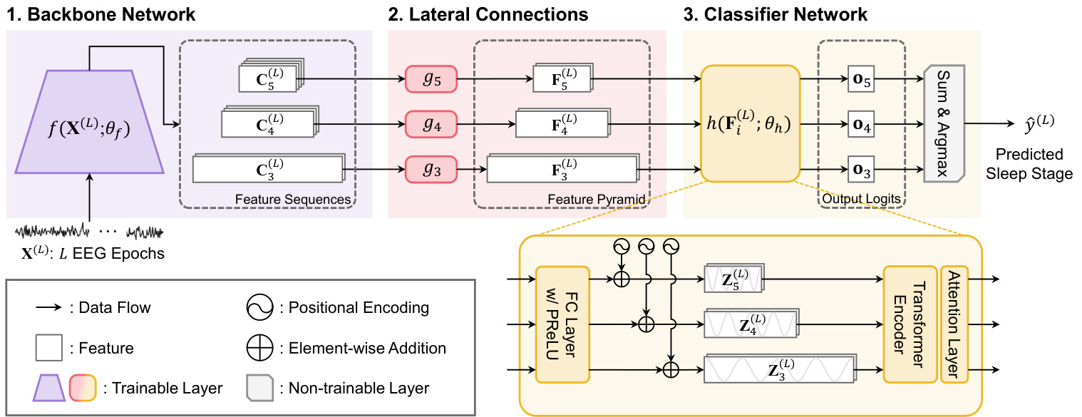
Figure 1: Model Architecture of SleePyCo. The purple, pink, and yellow regions indicate the backbone network, lateral connections, classifier network of $S l e e P y C o,$ and their corresponding outputs, respectively.
图 1: SleePyCo模型架构。紫色、粉色和黄色区域分别表示骨干网络、横向连接、$SleePyCo$的分类器网络及其对应输出。
Formally, SleePyCo-backbone takes $L$ successive EEG epochs as input, obtaining the following set of feature sequences:
形式上,SleePyCo-backbone 以 $L$ 个连续 EEG 时段作为输入,获得以下特征序列集合:
$$
{\mathbf{C}{3}^{(L)},\mathbf{C}{4}^{(L)},\mathbf{C}{5}^{(L)}}=f(\mathbf{X}^{(L)};\boldsymbol{\theta}_{f}),
$$
$$
{\mathbf{C}{3}^{(L)},\mathbf{C}{4}^{(L)},\mathbf{C}{5}^{(L)}}=f(\mathbf{X}^{(L)};\boldsymbol{\theta}_{f}),
$$
where $\mathbf{C}{i}^{(L)}$ denotes the output of the $i$ -th convolutional block of the backbone network, $f(\cdot)$ represents the backbone network, and $\theta_{f}$ indicates its trainable parameters. The size of the feature sequence can be denoted as Ci(L) $\mathbb{R}^{\lceil3000L/r_{i}\rceil\times c_{i}}$ , where $i\in{3,4,5}$ represents the stage index of the convolutional block, $c_{i}\in{192,256,256}$ denotes the feature dimension, $r_{i}\in{5^{2},5^{3},5^{4}}$ denotes the temporal reduction ratio, and $\lceil\cdot\rceil$ signifies the ceiling operation. Notably, the temporal reduction ratio $r_{i}$ is derived from the ratio of the length of the input $\mathbf{X}^{(L)}$ to that of the feature sequence $\mathbf{C}_{i}^{(L)}$ . The feature sequences from the first and second convolutional blocks were excluded from the feature pyramid owing to their large memory allocation. Thus, the stage indices of 1 and 2 were not considered in this study.
其中 $\mathbf{C}{i}^{(L)}$ 表示主干网络第 $i$ 个卷积块的输出,$f(\cdot)$ 代表主干网络,$\theta_{f}$ 表示其可训练参数。特征序列的尺寸可表示为 $\mathbb{R}^{\lceil3000L/r_{i}\rceil\times c_{i}}$,其中 $i\in{3,4,5}$ 表示卷积块的阶段索引,$c_{i}\in{192,256,256}$ 表示特征维度,$r_{i}\in{5^{2},5^{3},5^{4}}$ 表示时间缩减比率,$\lceil\cdot\rceil$ 表示向上取整运算。值得注意的是,时间缩减比率 $r_{i}$ 是由输入 $\mathbf{X}^{(L)}$ 长度与特征序列 $\mathbf{C}_{i}^{(L)}$ 长度的比值得出的。由于内存占用较大,第一和第二个卷积块的特征序列未被纳入特征金字塔,因此本研究未考虑阶段索引1和2。
2.2.2 Lateral Connections
2.2.2 横向连接
Lateral connections were attached at the end of the $3\mathrm{rd},$ $4\mathrm{th},$ and 5th convolutional blocks to form pyramidal feature sequences (i.e., feature pyramid) with identical feature dimensions. Importantly, the feature dimensions of the feature pyramid should be identical because all pyramidal feature sequences share a single classifier network. Because the feature vectors in the feature pyramid represent an assorted frequency meaning but the same semantic meaning (EEG patterns), the application of a shared classifier Ⅰis a pp ro pri ate in our methods. Formally, the feature pyramid ${\mathbf{F}{3}^{(L)},\mathbf{F}{4}^{(L)},\mathbf{F}_{5}^{(L)}}$ can be obtained using the following equation:
横向连接被附加在第3、第4和第5卷积块的末端,形成具有相同特征维度的金字塔特征序列(即特征金字塔)。重要的是,特征金字塔的特征维度应当保持一致,因为所有金字塔特征序列共享同一个分类器网络。由于特征金字塔中的特征向量代表不同的频率含义但相同的语义含义(EEG模式),在我们的方法中应用共享分类器是合适的。形式上,特征金字塔${\mathbf{F}{3}^{(L)},\mathbf{F}{4}^{(L)},\mathbf{F}_{5}^{(L)}}$可通过以下方程获得:
$$
\mathbf{F}{i}^{(L)}=g_{i}(\mathbf{C}{i}^{(L)};\theta_{g,i}),
$$
$$
\mathbf{F}{i}^{(L)}=g_{i}(\mathbf{C}{i}^{(L)};\theta_{g,i}),
$$
where $g_{i}(\cdot)$ denotes the lateral connection for the feature sequence Ci(L) w ith the trainable parameter $\theta_{g,i}$ . Each lateral connection consists of one convolutional layer with a filter width of 1 and results in a pyramidal feature sequence $\mathbf{F}{i}^{(L)}$ that describes the same temporal scale with $\mathbf{C}{i}^{({L})}$ . Thus, the size of the pyramidal feature sequences is formulated as Fi(L) ∈ R⌈3000L/ri⌉×df . In this study, the feature dimension $d_{f}$ was fixed at 128.
其中 $g_{i}(\cdot)$ 表示特征序列 $\mathbf{C}{i}^{(L)}$ 的横向连接,其可训练参数为 $\theta_{g,i}$。每个横向连接由一个滤波器宽度为1的卷积层组成,并生成金字塔特征序列 $\mathbf{F}{i}^{(L)}$,该序列与 $\mathbf{C}{i}^{(L)}$ 具有相同的时间尺度。因此,金字塔特征序列的尺寸可表示为 $\mathbf{F}_{i}^{(L)} \in \mathbb{R}^{\lceil 3000L/r_i \rceil \times d_f}$。本研究中,特征维度 $d_f$ 固定为128。
2.2.3 Classifier Network
2.2.3 分类器网络
The classifier network of $S l e e P y C o$ can analyze the temporal context in the feature pyramid and output the predicted sleep stage of the target epoch $\hat{y}^{(L)}$ . Formally, we denote the classifier network as $h(\bar{\mathbf{F}{i}^{(L)}};\boldsymbol{\theta_{h}}).$ , where $\theta_{h}$ is the trainable parameter. We utilized the encoder part of the Transformer [49] for sequential modelling of the feature pyramid extracted from the raw single-channel EEG. Overall, recurrent architectures such as LSTM [50] and GRU [51] were widely adopted in automatic sleep scoring. Interestingly, the transformer delivered a remarkable performance in various sequential modeling tasks, including automatic sleep scoring [27], [28], [52]. Owing to the large number of parameters of the original transformer, we reduced the model dimension $d_{m}$ (i.e., dimension of the queue, value, and query) and the feed-forward network dimension $d_{F F}$ in comparison to the original ones. We used the original configuration of the number of heads $N_{h}$ and the number of encoder layers $N_{e}$ . The parameters are detailed in Section 4.3.
$S l e e P y C o$ 的分类器网络能够分析特征金字塔中的时序上下文,并输出目标时段 $\hat{y}^{(L)}$ 的预测睡眠阶段。形式上,我们将分类器网络表示为 $h(\bar{\mathbf{F}{i}^{(L)}};\boldsymbol{\theta_{h}})$ ,其中 $\theta_{h}$ 为可训练参数。我们采用 Transformer [49] 的编码器部分对从原始单通道 EEG 提取的特征金字塔进行序列建模。总体而言,LSTM [50] 和 GRU [51] 等循环架构在自动睡眠评分中被广泛采用。有趣的是,Transformer 在包括自动睡眠评分 [27]、[28]、[52] 在内的多种序列建模任务中表现出色。由于原始 Transformer 参数量较大,我们降低了模型维度 $d_{m}$ (即队列、值和查询的维度)和前馈网络维度 $d_{F F}$ ,同时保留了头数 $N_{h}$ 和编码器层数 $N_{e}$ 的原始配置。具体参数详见第 4.3 节。
Prior to the transformer encoder, a shared fully connected layer with PReLU is employed to transform the feature dimension of the feature pyramid into the dimension of the transformer encoder. Specifically, we denote the transformed feature pyramid as F(L) $\mathbf{\tilde{F}}{i}^{(L)}\in\mathbf{\bar{\mathbb{R}}}^{\lceil3000L/r_{i}\rceil\times d_{m}}$ . This layer maps EEG patterns from various convolutional stages into the same feature space, and thus, the shared classifier considers the temporal context, regardless of the feature level. Subsequently, because the transformer encoder is a recurrent-free architecture, the positional encoding $\mathbf{P}{i}^{(L)}\in\mathbb{R}^{\lceil3000L/r_{i}\rceil\times d_{m}}$ should be added to the input feature sequences to blend the temporal information:
在Transformer编码器之前,采用带有PReLU的共享全连接层将特征金字塔的特征维度转换为Transformer编码器的维度。具体而言,我们将转换后的特征金字塔表示为F(L) $\mathbf{\tilde{F}}{i}^{(L)}\in\mathbf{\bar{\mathbb{R}}}^{\lceil3000L/r_{i}\rceil\times d_{m}}$ 。该层将来自不同卷积阶段的EEG模式映射到相同的特征空间,因此共享分类器会考虑时间上下文,而不受特征层级的影响。随后,由于Transformer编码器是一种无循环架构,需要将位置编码 $\mathbf{P}{i}^{(L)}\in\mathbb{R}^{\lceil3000L/r_{i}\rceil\times d_{m}}$ 添加到输入特征序列中以融合时序信息:
$$
\mathbf{Z}{i}^{(L)}=\tilde{\mathbf{F}}{i}^{(L)}+\mathbf{P}_{i}^{(L)},
$$
$$
\mathbf{Z}{i}^{(L)}=\tilde{\mathbf{F}}{i}^{(L)}+\mathbf{P}_{i}^{(L)},
$$
where $\mathbf{P}{i}^{(L)}\in\mathbb{R}^{\lceil3000L/r_{i}\rceil\times d_{m}}$ denotes the positional encoding matrix for the $i$ -th feature sequence. Herein, sinusoidal positional encoding was performed following a prior study [49]. However, because the same time indices are applicable at both ends of the pyramidal feature sequences, we modified the positional encoding to coincide with the absolute temporal position between them by hopping the temporal index of positional encoding. Thus, the element of $\mathbf{P}_{i}^{(L)}$ at the temporal index $t$ and dimension index $k$ can be defined as
其中 $\mathbf{P}{i}^{(L)}\in\mathbb{R}^{\lceil3000L/r_{i}\rceil\times d_{m}}$ 表示第 $i$ 个特征序列的位置编码矩阵。此处采用正弦位置编码方法 [49]。由于金字塔特征序列两端具有相同的时间索引,我们通过跳跃位置编码的时间索引,将其修改为与两者之间的绝对时间位置对齐。
where $\lfloor\cdot\rfloor$ denotes the floor operation and $\textit{R}=\left.r_{i}/r_{i-1}\right.$ indicates a temporal reduction factor (set as 5 in this study). $\mathbf{P}_{i}^{(L)}(t,k)$ degenerates into the original sinusoidal positional encoding for $i=3$ .
其中 $\lfloor\cdot\rfloor$ 表示向下取整运算,$\textit{R}=\left.r_{i}/r_{i-1}\right.$ 表示时间缩减因子(本研究设为5)。当 $i=3$ 时,$\mathbf{P}_{i}^{(L)}(t,k)$ 退化为原始正弦位置编码。
The output hidden states $\mathbf{H}{i}^{(L)}\in\mathbb{R}^{\lceil3000L/r_{i}\rceil\times d_{m}}$ for the $i$ -th pyramidal feature sequence can be formulated as
第 $i$ 个金字塔特征序列的隐藏状态输出 $\mathbf{H}{i}^{(L)}\in\mathbb{R}^{\lceil3000L/r_{i}\rceil\times d_{m}}$ 可表示为
$$
\mathbf{H}{i}^{(L)}=\mathrm{TransformerEncoder}(\mathbf{Z}_{i}^{(L)}),
$$
$$
\mathbf{H}{i}^{(L)}=\mathrm{TransformerEncoder}(\mathbf{Z}_{i}^{(L)}),
$$
where Transformer Encoder $\cdot(\cdot)$ denotes the encoder component of the transformer. To integrate the output hidden states at various time steps into a single feature vector, we utilized the attention layer [53] [54] as [17]. Foremostly, the output hidden states Hi(L) were projected into the attentional hidden states Ai(L) $\mathbf{A}{i}^{(L)}={\mathbf{a}{i,1},\mathbf{a}{i,2},...,\mathbf{a}{i,T_{i}}},$ , where $T_{i}$ is $\left\lceil3000L/r_{i}\right\rceil.$ , via a single fully-connected layer. Thereafter, the attention al feature vector $\bar{\mathbf{a}}{i}$ of the $i$ -th pyramidal feature sequence can be formulated via a weighted summation of $\mathbf{a}_{i,t}$ along the temporal dimension:
其中Transformer Encoder $\cdot(\cdot)$ 表示Transformer的编码器组件。为了将不同时间步的输出隐藏状态整合为单一特征向量,我们采用了注意力层[53][54]如[17]所述。首先,将输出隐藏状态Hi(L)投影为注意力隐藏状态Ai(L) $\mathbf{A}{i}^{(L)}={\mathbf{a}{i,1},\mathbf{a}{i,2},...,\mathbf{a}{i,T_{i}}},$ ,其中$T_{i}$为$\left\lceil3000L/r_{i}\right\rceil.$ ,通过单个全连接层实现。随后,第$i$个金字塔特征序列的注意力特征向量$\bar{\mathbf{a}}{i}$可通过沿时间维度对$\mathbf{a}_{i,t}$进行加权求和得到:
this function is defined as
该函数定义为
$$
s(\mathbf{a})=\mathbf{a}\mathbf{W}_{\mathrm{att}},
$$
$$
s(\mathbf{a})=\mathbf{a}\mathbf{W}_{\mathrm{att}},
$$
where $\mathbf{W}{\mathrm{att}}\in\mathbb{R}^{d_{m}\times1}$ represents the trainable parameter.
其中 $\mathbf{W}{\mathrm{att}}\in\mathbb{R}^{d_{m}\times1}$ 表示可训练参数。
Upon using the attention feature vector a obtained from Eq. 6, the output logits of the $i$ -th pyramidal feature sequence, $\mathbf{o}_{i}$ , can be formulated as follows:
在使用从公式6获得的注意力特征向量a后,第i个金字塔特征序列的输出logits $\mathbf{o}_{i}$ 可表示为:
$$
\mathbf{o}{i}=\bar{\mathbf{a}}{i}\mathbf{W}{\mathrm{a}}+\mathbf{b}_{\mathrm{a}},
$$
$$
\mathbf{o}{i}=\bar{\mathbf{a}}{i}\mathbf{W}{\mathrm{a}}+\mathbf{b}_{\mathrm{a}},
$$
where ${\mathbf W}{\mathrm{a}}\in\mathbb{R}^{d_{m}\times N_{c}}$ and $\mathbf{b}{\mathrm{a}}\in\mathbb{R}^{1\times N_{c}}$ denote the trainable weight and bias, respectively. Eventually, the sleep stage $\hat{y}^{(L)}$ of the target epoch was predicted based on the following relation.
其中 ${\mathbf W}{\mathrm{a}}\in\mathbb{R}^{d_{m}\times N_{c}}$ 和 $\mathbf{b}{\mathrm{a}}\in\mathbb{R}^{1\times N_{c}}$ 分别表示可训练的权重和偏置。最终,目标时段的睡眠阶段 $\hat{y}^{(L)}$ 通过以下关系式进行预测。
$$
\hat{y}^{(L)}=\operatorname{argmax}(\sum_{i\in{3,4,5}}\mathbf{o}_{i}),
$$
$$
\hat{y}^{(L)}=\operatorname{argmax}(\sum_{i\in{3,4,5}}\mathbf{o}_{i}),
$$
where argmax $(\cdot)$ is the operation that returns the index of the maximum value.
其中 argmax $(\cdot)$ 是返回最大值索引的操作。
3 SUPERVISED CONTRASTIVE LEARNING
3 监督对比学习
As illustrated in Fig. 2, our learning framework involves two training steps. The first step involves contrastive representation learning (CRL) to pretrain the backbone network $f(\cdot)$ via a contrastive learning strategy. In this step, the backbone network $f(\cdot)$ is trained to extract the class disc rim i native features based on the supervised contrastive loss [43]. The second step involves multiscale temporal context learning (MTCL) to learn sequential relations in feature pyramid. For this purpose, we acquire the learned weights of $f(\cdot)$ from CRL and freeze them to conserve the class disc rim i native features. The remaining parts of the network $(g(\cdot)$ and $h(\cdot))$ are trained to learn the multiscale temporal context by predicting the sleep stage of the target epoch.
如图 2 所示,我们的学习框架包含两个训练步骤。第一步通过对比表示学习 (contrastive representation learning, CRL) ,采用对比学习策略对主干网络 $f(\cdot)$ 进行预训练。在此步骤中,主干网络 $f(\cdot)$ 基于监督对比损失 [43] 学习提取类别判别特征。第二步通过多尺度时序上下文学习 (multiscale temporal context learning, MTCL) 在特征金字塔中学习序列关系。为此,我们从 CRL 中获取 $f(\cdot)$ 的已学习权重并冻结它们以保留类别判别特征。网络的其余部分 $(g(\cdot)$ 和 $h(\cdot))$ 则通过预测目标时相的睡眠阶段来学习多尺度时序上下文。
To prevent over fitting during the training procedures, we performed early stopping in both CRL and MTCL. Thus, validation was performed to track the validation cost (i.e., validation loss) at every certain training iteration (i.e., validation period, $\psi,$ ), and the training was terminated if the validation loss did not progress more than a certain number of times (i.e., early stopping patience, $\phi)$ . Early stopping in supervised contrastive learning (SCL) results in better pretrained parameters of the backbone network and prevents over fitting at the $M T C L$ step. The details of the hyper parameters used in $S C L$ are summarized in Section 4.4. Note that different validation periods, $\psi_{1}$ and $\psi_{2},$ were used in $C R L$ and $M T C L,$ , respectively. The specifics of the training framework are described in the following sections and Algorithm 1.
为防止训练过程中出现过拟合,我们在CRL和MTCL中均采用了早停机制。具体而言,通过验证集定期(即验证周期$\psi$)跟踪验证成本(即验证损失),若验证损失连续超过特定次数(即早停耐心值$\phi$)未改善,则终止训练。监督对比学习(SCL)中的早停机制可获得主干网络更优的预训练参数,并避免MTCL步骤中的过拟合。SCL所用超参数详情见第4.4节。需注意CRL与MTCL分别采用不同的验证周期$\psi_{1}$和$\psi_{2}$。训练框架的具体实现详见下文及算法1。
$$
\bar{\mathbf{a}}{i}=\sum_{t=1}^{T_{i}}\alpha_{i,t}\mathbf{a}_{i,t},
$$
where the attention weight $\alpha_{i,t}$ at time step $t$ is derived by
其中时间步 $t$ 的注意力权重 $\alpha_{i,t}$ 由
$$
\alpha_{i,t}=\frac{\exp(s(\mathbf{a}{i,t}))}{\sum_{t}\exp(s(\mathbf{a}_{i,t}))},
$$
$$
\alpha_{i,t}=\frac{\exp(s(\mathbf{a}{i,t}))}{\sum_{t}\exp(s(\mathbf{a}_{i,t}))},
$$
where $s(\cdot)$ denotes the attention scoring function that maps the attention al hidden state into a scalar value. Formally,
其中 $s(\cdot)$ 表示将注意力隐藏状态映射为标量值的注意力评分函数。形式上,
3.1 Contrastive Representation Learning
3.1 对比表征学习 (Contrastive Representation Learning)
In $C R L,$ , we implemented the training strategy of SCL [43] to extract the class disc rim i native features from a single EEG epoch. As illustrated in Fig. 2-(a), the CRL aimed to maximize the similarity between the two projected vectors based on two different views of a single EEG epoch. Simultaneously, the similarity between two projected vectors from different sleep stages was minimized as the optimization of supervised contrastive loss. Thus, we focused on reducing the ambiguous frequency characteristics by extracting dist ingui sh able representations of the sleep stage. Accordingly, a single EEG epoch was initially transformed by two distinct augmentation functions. Thereafter, the encoder network and projection network mapped them into the hyper sphere, which produced a latent vector $_{z}$ . The details are explained in the following sections: Augmentation Module, Encoder Network, Projection Network, and Loss Function, which constitute the major components of CRL.
在 $C R L,$ 中,我们采用了SCL [43] 的训练策略,从单个脑电图 (EEG) 时段中提取类别判别特征。如图 2-(a) 所示,CRL旨在基于单个EEG时段两种不同视角的投影向量最大化其相似性。同时,来自不同睡眠阶段的投影向量间的相似性被最小化,作为监督对比损失 (supervised contrastive loss) 的优化目标。因此,我们通过提取可区分的睡眠阶段表征来减少模糊的频率特征。具体而言,单个EEG时段首先通过两种不同的增强函数进行转换。随后,编码器网络和投影网络将其映射至超球面空间,生成潜在向量 $_{z}$ 。以下章节将详细说明构成CRL核心的模块:增强模块、编码器网络、投影网络和损失函数。
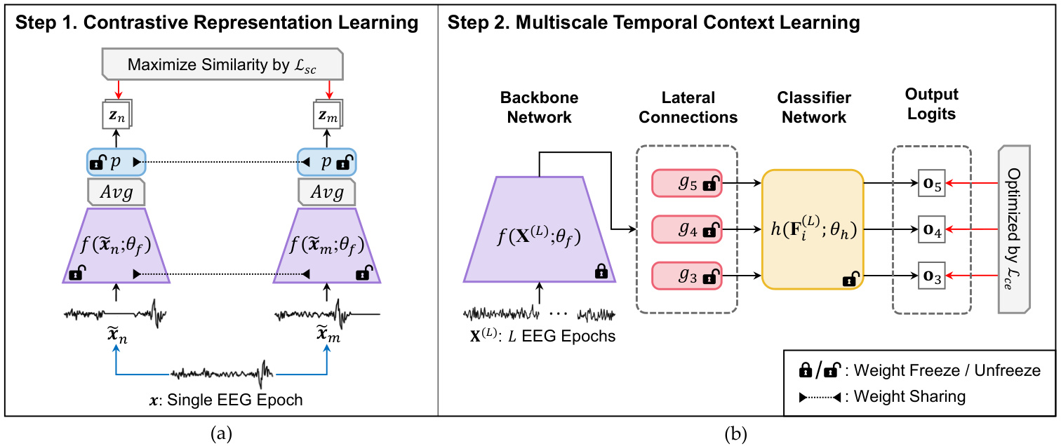
Figure 2: Illustration of the proposed supervised contrastive learning framework. (a) Contrastive representation learning (CRL); (b) multiscale temporal context learning (MTCL); red arrow is first backward path and blue arrow is $A u g(\cdot)$ .
图 2: 提出的监督对比学习框架示意图。(a) 对比表征学习(CRL); (b) 多尺度时序上下文学习(MTCL); 红色箭头为首次反向路径, 蓝色箭头为 $A u g(\cdot)$。
Data Augmentation Module: The data augmentation module, $A u g(\cdot).$ , transforms a single epoch of EEG signal $_{x}$ into a slightly different but semantically identical signal as follows:
数据增强模块:数据增强模块 $Aug(\cdot)$ 将单段脑电图信号 $_{x}$ 转换为语义相同但略有差异的信号,具体如下:
$$
\tilde{\pmb{x}}={\cal A}u g({\pmb x}),
$$
$$
\tilde{\pmb{x}}={\cal A}u g({\pmb x}),
$$
where $\tilde{x}$ denotes a different perspective on a single EEG epoch ${x}$ . With a given set of randomly sampled data ${\pmb{x}{p},\pmb{y}{p}}{p=1,\dots,N_{b}}$ (i.e., batch), two different augmentations result in ${\tilde{x}{q},\tilde{y}{q}}{q=1,\dots,2N_{b}.}$ , called a multi viewed batch [43] as illustrated in Fig. 2-(a), where $N_{b}$ is the batch size and $\tilde{y}{2p-1}=\tilde{y}{2p}=y_{p}$ . Because the augmentation set is crucial for contrastive learning, we adopted the verified transformation functions from previous studies [23], [33]. As listed in Table 1, we sequentially applied six transformations, namely, amplitude scale, time shift, amplitude shift, zero-masking, additive Gaussian noise, and band-stop filter with the probability of 0.5. In addition, we modified the hyperparameter of the transformation functions by considering the sampling rate and characteristics of the EEG signal.
其中 $\tilde{x}$ 表示对单个脑电图(EEG)时段 ${x}$ 的不同视角。给定一组随机采样的数据 ${\pmb{x}{p},\pmb{y}{p}}{p=1,\dots,N_{b}}$ (即批次),两种不同的增强操作会生成 ${\tilde{x}{q},\tilde{y}{q}}{q=1,\dots,2N_{b}.}$,称为多视角批次[43],如图2-(a)所示。这里 $N_{b}$ 是批次大小,且 $\tilde{y}{2p-1}=\tilde{y}{2p}=y_{p}$。由于增强集对对比学习至关重要,我们采用了先前研究[23][33]中已验证的变换函数。如表1所列,我们依次应用了六种变换:幅度缩放、时间偏移、幅度偏移、零掩码、加性高斯噪声和带阻滤波器,每种变换的应用概率为0.5。此外,我们还根据EEG信号的采样率和特性修改了变换函数的超参数。
Encoder Network: The encoder network transforms an augmented single-EEG epoch $\tilde{x}$ into a representation vector $\pmb{r}\in\mathbb{R}^{c_{5}}$ . The encoder network contains the sequence of the backbone network $f(\cdot)$ and the global average pooling operation $A v g(\cdot)$ . Thus, the backbone network initially transforms an augmented single-EEG epoch $\tilde{x}$ into the feature sequence $\mathbf{F}{5}^{(\mathrm{1})}$ . Then, the representation vector is obtained from the feature sequence via global average pooling along the temporal dimension. Formally, the representation vector is evaluated as $r=A v g(\mathbf{F}_{5}^{(1)})$ .
编码器网络:编码器网络将增强的单个脑电图时段 $\tilde{x}$ 转换为表示向量 $\pmb{r}\in\mathbb{R}^{c_{5}}$。该网络由骨干网络 $f(\cdot)$ 和全局平均池化操作 $A v g(\cdot)$ 依次组成。具体而言,骨干网络首先将增强的单个脑电图时段 $\tilde{x}$ 转换为特征序列 $\mathbf{F}{5}^{(\mathrm{1})}$,随后通过沿时间维度进行全局平均池化得到表示向量。其数学表达式为 $r=A v g(\mathbf{F}_{5}^{(1)})$。
Table 1: Data Augmentation Pipeline
表 1: 数据增强流程
| TransformationPipeline | Min | Max | Probability |
|---|---|---|---|
| amplitude scaling | 0.5 | 2 | 0.5each |
| time shift (samples) | -300 | 300 | 0.5each |
| amplitude shift (μV) | -10 | 10 | 0.5each |
| zero-masking (samples) | 0 | 300 | 0.5each |
| additiveGaussiannoise(o) | 0 | 0.2 | 0.5each |
| band-stop filter (2 Hz width) (lower bound frequency,Hz) | 0.5 | 30.0 | 0.5each |
Projection Network: The projection network is vital for mapping the representation vector $r$ into the normalized latent vector z = $\begin{array}{r}{z=\frac{z^{\prime}}{|z^{\prime}|{2}}\in\mathbb{R}^{d_{z}},}\end{array}$ , where $z^{\prime}=p(r;\theta_{p}),p(\cdot)$ denotes the projection network, $\theta_{p}$ represents its trainable parameter, and $d_{z}$ indicates the dimension of the latent vector. We use a multilayer perceptron [55] with a single hidden layer of size 128 to obtain a latent vector of size $d_{z}=128$ as the projection network. For sequential modeling, the $p(\cdot)$ is removed at the MTCL.
投影网络 (Projection Network):该网络对于将表示向量 $r$ 映射到归一化潜在向量 z = $\begin{array}{r}{z=\frac{z^{\prime}}{|z^{\prime}|{2}}\in\mathbb{R}^{d_{z}},}\end{array}$ 至关重要。其中 $z^{\prime}=p(r;\theta_{p})$,$p(\cdot)$ 表示投影网络,$\theta_{p}$ 代表其可训练参数,$d_{z}$ 表示潜在向量的维度。我们采用具有单个128维隐藏层的多层感知机 [55] 作为投影网络,最终获得维度为 $d_{z}=128$ 的潜在向量。在序列建模时,MTCL 层会移除 $p(\cdot)$ 功能。
Loss Function: For $C R L,$ we adopt the supervised contrastive loss proposed in [43]. The supervised contrastive loss simultaneously maximizes the similarity between positive pairs and promotes the deviations across negative pairs. In this study, samples annotated with the same sleep stage in a multi viewed batch are regarded as positives, and negatives otherwise. Formally, the supervised contrastive loss function can be formulated as
损失函数:对于$CRL$,我们采用[43]提出的监督对比损失。该损失函数同时最大化正样本对的相似性,并扩大负样本对之间的差异。本研究中,在多视角批次中标注为相同睡眠阶段的样本被视为正样本,其余为负样本。形式上,监督对比损失函数可表述为
$$
\mathcal{L}{s c}=-\sum_{n=1}^{2N_{b}}\frac{1}{N_{p}^{(n)}}\sum_{m=1}^{2N_{b}}\log\frac{\mathbb{1}{[n\neq m]}\mathbb{1}{[\tilde{y}{n}=\tilde{y}{m}]}\exp(z_{n}\cdot z_{m}/\tau)}{\sum_{a=1}^{2N_{b}}\mathbb{1}{[n\neq a]}\exp(z_{n}\cdot z_{a}/\tau)},
$$
$$
\mathcal{L}{s c}=-\sum_{n=1}^{2N_{b}}\frac{1}{N_{p}^{(n)}}\sum_{m=1}^{2N_{b}}\log\frac{\mathbb{1}{[n\neq m]}\mathbb{1}{[\tilde{y}{n}=\tilde{y}{m}]}\exp(z_{n}\cdot z_{m}/\tau)}{\sum_{a=1}^{2N_{b}}\mathbb{1}{[n\neq a]}\exp(z_{n}\cdot z_{a}/\tau)},
$$
where $N_{p}^{(n)}$ denotes the number of positives for the $n$ -th sample in a multi viewed batch excluding itself, $\mathbb{1}{[\cdot]}$ denotes the indicator function, $\tilde{{\pmb y}}{n}$ denotes the ground truth corresponding to $z_{n},$ · operation denotes the inner product between two vectors, and $\tau\in\mathbb{R}^{+}$ denotes a scalar temperature parameter $\mathrm{\Delta}\tau=0.07$ in all present experiments).
其中 $N_{p}^{(n)}$ 表示多视角批次中第 $n$ 个样本除自身外的正样本数量,$\mathbb{1}{[\cdot]}$ 表示指示函数,$\tilde{{\pmb y}}{n}$ 表示与 $z_{n}$ 对应的真实标签,· 运算表示两个向量的内积,$\tau\in\mathbb{R}^{+}$ 表示标量温度参数(当前所有实验中 $\mathrm{\Delta}\tau=0.07$)。
3.2 Multiscale Temporal Context Learning
3.2 多尺度时序上下文学习
As illustrated in Fig. 2-(b), the second step of SleePyCo executes $L$ successive EEG epochs $\mathbf{\boldsymbol{x}}^{(L)}$ to analyze both the intra- and inter-epoch temporal contexts $\mathit{\Delta}L=10$ in this study). The performance obtained considering intra- and inter-epoch temporal contexts [15] is better than that considering only the intra-epoch. However, it is difficult for the network to capture the EEG patterns of the previous epochs, because only the label of the target epoch is provided. To resolve this, we fixed the parameters of the backbone network $f(\cdot)$ to maintain and utilize the class disc rim i native features learned from CRL. By contrast, the remaining parts of the network, which are lateral connections $g(\cdot)$ and classifier network $h(\cdot)$ , are learned to score the sleep stage of the target epoch based on the following loss function:
如图 2-(b) 所示,SleePyCo 的第二步执行 $L$ 个连续的 EEG 时段 $\mathbf{\boldsymbol{x}}^{(L)}$ 来分析时段内和时段间的时间上下文 (本研究设定 $\mathit{\Delta}L=10$)。考虑时段内和时段间时间上下文的性能 [15] 优于仅考虑时段内上下文的情况。然而,由于仅提供了目标时段的标签,网络难以捕捉先前时段的 EEG 模式。为解决这一问题,我们固定了骨干网络 $f(\cdot)$ 的参数,以保持并利用从 CRL 中学到的类别判别特征。相比之下,网络的其余部分 (横向连接 $g(\cdot)$ 和分类器网络 $h(\cdot)$) 则通过学习以下损失函数来对目标时段的睡眠阶段进行评分:
$$
\mathcal{L}{c e}=-\sum_{i\in{3,4,5}}\sum_{j=1}^{N_{c}}y_{j}^{(L)}\log\left(\frac{\exp(o_{i,j})}{\sum_{k=1}^{N_{c}}\exp(o_{i,k})}\right),
$$
$$
\mathcal{L}{c e}=-\sum_{i\in{3,4,5}}\sum_{j=1}^{N_{c}}y_{j}^{(L)}\log\left(\frac{\exp(o_{i,j})}{\sum_{k=1}^{N_{c}}\exp(o_{i,k})}\right),
$$
where yj $y_{j}^{(L)}$ ) denotes the $j$ -th element of one-hot encoding label, and $o_{i,j}$ represents the $j$ -th element of output logits from the $i$ -th convolutional stage. This loss function follows the summation of cross entropy over the output logits from each convolutional block.
其中 ( y_{j}^{(L)} ) 表示独热编码标签的第 ( j ) 个元素,( o_{i,j} ) 表示第 ( i ) 个卷积阶段输出 logits 的第 ( j ) 个元素。该损失函数对每个卷积块的输出 logits 进行交叉熵求和。
Because all pyramidal feature sequences share a single classifier network, the classifier network considers feature sequences across a broad scale. Thus, Eq. 13 facilitates the classifier network to analyze the temporal relation between the EEG patterns at different temporal scales and frequency characteristics. Consequently, the classifier network $h(\cdot)$ models the temporal information based on the pyramidal feature sequences Fi(L) derived from analyzing the intraand inter-epoch temporal contexts.
由于所有金字塔特征序列共享同一个分类器网络,该网络能够考虑跨广泛尺度的特征序列。因此,式13促使分类器网络分析不同时间尺度和频率特性下脑电图(EEG)模式之间的时序关系。最终,分类器网络$h(\cdot)$基于从分析时段内和时段间时序上下文得到的金字塔特征序列Fi(L)来建模时序信息。
4 EXPERIMENTS
4 实验
4.1 Datasets
4.1 数据集
Four public datasets, including PSG recordings and their associated sleep stages, were utilized to assess the performance of SleePyCo: Sleep-EDF (2018 version), Montreal Archive of Sleep Studies (MASS), Ph y sion et 2018, and Sleep Heart Health Study (SHHS). The number of subjects, utilized EEG channels, evaluation scheme, number of held-out validation subjects, and sample distribution are presented in Table 2. In this study, all EEG signals except the Sleep-EDF dataset were down sampled to $100~\mathrm{Hz}$ . We did not employ preprocessing to EEG signals except for down sampling. For all datasets, we discarded the EEG epochs with annotations that were not related to the sleep stage, such as MOVEMENT class. In addition, we merged N3 and N4 into N3 to consider the five-class problem for datasets annotated with R&K [4].
为评估SleePyCo的性能,研究使用了四个包含PSG记录及对应睡眠分期的公开数据集:Sleep-EDF(2018版)、蒙特利尔睡眠研究档案库(MASS)、Physionet 2018以及睡眠心脏健康研究(SHHS)。表2展示了各数据集的受试者数量、使用的EEG通道、评估方案、预留验证集人数及样本分布情况。本研究中,除Sleep-EDF数据集外,所有EEG信号均降采样至$100~\mathrm{Hz}$,且除降采样外未进行其他预处理。对于所有数据集,我们剔除了标注与睡眠分期无关的EEG时段(如MOVEMENT类)。此外,为将R&K[4]标注数据集统一为五分类问题,我们将N3与N4阶段合并为N3。
Sleep-EDF: The Sleep-EDF Expanded dataset [44], [45] (2018 version) includes 197 PSG recordings containing EEG, EOG, chin EMG, and event markers. The Sleep-EDF dataset
Sleep-EDF:Sleep-EDF扩展数据集[44][45](2018版)包含197份PSG记录,涵盖脑电图(EEG)、眼电图(EOG)、下颌肌电图(EMG)及事件标记。
Algorithm us 1 Training Algorithm
算法1 训练算法
comprises two kinds of studies: SC for 79 healthy Caucasian individuals without sleep disorders and ST for 22 subjects of a study on the effects of Temazepam on sleep. In this study, the SC recordings (subjects aged 25–101 years) were used based on previous studies [7], [17], [21], [25], [27]. According to the R&K rule [4], sleep experts score each halfminute epoch with one of the eight classes {WAKE, REM, N1, N2, N3, N4, MOVEMENT, UNKNOWN}. Owing to the larger size of the class WAKE group compared to others, we included only 30 min of WAKE epochs before and after the sleep period.
包含两类研究:SC针对79名无睡眠障碍的健康白种人,ST针对22名受试者进行替马西泮对睡眠影响的研究。本研究中,基于先前研究[7]、[17]、[21]、[25]、[27],采用了SC记录(受试者年龄25-101岁)。根据R&K规则[4],睡眠专家将每半分钟时段划分为八种类别之一{清醒(WAKE)、快速眼动睡眠(REM)、N1、N2、N3、N4、体动(MOVEMENT)、未知(UNKNOWN)}。由于清醒(WAKE)类别的样本量显著大于其他类别,我们仅纳入睡眠周期前后各30分钟的清醒时段数据。
MASS: The Montreal Archive of Sleep Studies (MASS) dataset [56] contains PSG recordings from 200 individuals (97 males and 103 females). This dataset includes five subsets (SS1, SS2, SS3, SS4, and SS5) that are classified based on the research purpose and data acquisition protocols. The AASM standard [5] (SS1 and SS3 subsets) or the R&K standard [4] (SS2, SS4, and SS5 subsets) was used for the manual annotation. Specifically, the SS1, SS2, and SS4 subsets were annotated with 20-s EEG epochs instead of SS3 and SS5 subsets. Because 30-s EEG samples are used in SCL, 5-s segments of signals before and after the EEG epoch were considered for the case of SS1, SS2, and SS4. In MTCL, an equal length of EEG signals was used for all subsets $(300~\mathrm{s}$ in this study).
MASS: Montreal睡眠研究档案库 (MASS) 数据集 [56] 包含200名受试者 (97名男性和103名女性) 的PSG记录。该数据集包含五个子集 (SS1、SS2、SS3、SS4和SS5),根据研究目的和数据采集协议进行分类。手动标注采用AASM标准 [5] (SS1和SS3子集) 或R&K标准 [4] (SS2、SS4和SS5子集)。具体而言,SS1、SS2和SS4子集采用20秒EEG时段进行标注,而SS3和SS5子集则未采用。由于SCL使用30秒EEG样本,对于SS1、SS2和SS4的情况,考虑了EEG时段前后5秒的信号段。在MTCL中,所有子集使用相同长度的EEG信号 (本研究中为$300~\mathrm{s}$)。
Table 2: Experimental settings and dataset statistics
表 2: 实验设置与数据集统计
| 数据集 | 受试者数量 | EEG | 实验设置 | 保留验证集 | 清醒 | N1 | N2 | N3 | REM | 总计 |
|---|---|---|---|---|---|---|---|---|---|---|
| Sleep-EDF | 79 | Fpz-Cz | 10折交叉验证 | 7名受试者 | 69,824 (35.8%) | 21,522 (10.8%) | 69,132 (34.7%) | 13,039 (6.5%) | 25,835 (13.0%) | 199,352 |
| MASS | 200 | C4-A1 | 20折交叉验证 | 10名受试者 | 31,184 (13.6%) | 19,359 (8.5%) | 107,930 (47.1%) | 30,383 (13.3%) | 40,184 (17.5%) | 229,040 |
| Physio2018 | 994 | C3-A2 | 5折交叉验证 | 50名受试者 | 157,945 (17.7%) | 136,978 (15.4%) | 377,870 (42.3%) | 102,592 (11.5%) | 116,877 (13.1%) | 892,262 |
| SHHS | 5,793 | C4-A1 | 训练/测试:0.7:0.3 | 100名受试者 | 1,691,288 (28.8%) | 217,583 (3.7%) | 2,397,460 (40.9%) | 739,403 (12.6%) | 817,473 (13.9%) | 5,863,207 |
Physio2018: The Physio2018 dataset is contributed by the Computational Clinical Neuro physiology Laboratory at Massachusetts General Hospital and was applied to detect arousal during sleep in the 2018 Physionet challenge [44], [57]. Owing to the un availability of annotation for the evaluation set, we used the training set containing PSG recordings for 994 subjects aged 18–90. Thereafter, these recordings were annotated with the AASM rules [5], and we employed only C3–A2 EEG recordings for the singlechannel EEG classification.
Physio2018:Physio2018数据集由马萨诸塞州总医院计算临床神经生理学实验室贡献,用于2018年Physionet挑战赛中检测睡眠期间的觉醒状态[44][57]。由于评估集缺乏标注,我们使用了包含994名18-90岁受试者的PSG记录训练集。这些记录随后按照AASM规则[5]进行标注,在单通道EEG分类中仅采用C3-A2导联的EEG记录。
SHHS: The SHHS dataset [58], [59] is a multi center cohort research that is designed to examine the influence of sleep apnea on cardiovascular diseases. The collection is composed of two rounds of PSG records: Visit 1 (SHHS-1) and Visit 2 (SHHS-2), wherein each record contains twochannel EEGs, two-channel EOGs, a single-channel EMG, a single-channel ECG, and two-channel respiratory inductance ple thys mo graph y, as well as the data from location sensors, light sensors, pulse oximeters, and airflow sensors. Each epoch was assigned a value of W, REM, N1, N2, N3, N4, MOVEMENT, and UNKNOWN according to the R&K rule [4]. In this study, the single-channel EEG (C4–A1) was analyzed from 5,793 SHHS-1 recordings.
SHHS: SHHS数据集[58][59]是一项多中心队列研究,旨在探究睡眠呼吸暂停对心血管疾病的影响。该数据集包含两轮PSG记录:第一次访问(SHHS-1)和第二次访问(SHHS-2),每条记录均包含双通道脑电图(EEG)、双通道眼电图(EOG)、单通道肌电图(EMG)、单通道心电图(ECG)、双通道呼吸感应体积描记信号,以及定位传感器、光传感器、脉搏血氧仪和气流传感器的数据。根据R&K规则[4],每个时段被标记为W、REM、N1、N2、N3、N4、MOVEMENT或UNKNOWN值。本研究从5,793份SHHS-1记录中提取单通道脑电图(C4–A1)进行分析。
4.2 Backbone Networks for Ablation Study
4.2 消融实验的骨干网络
A direct comparison between the automatic sleep scoring methods would not be justified depending on the experimental settings such as the data processing method and training framework. For fair comparison with other stateof-the-art backbones, we implemented four backbones in the current training framework: Deep Sleep Net [16], IITNet [15], U-Time [25], and XSleepNet [7]. The backbones were trained and evaluated in the proposed framework on the same datasets (Sleep-EDF, MASS, Physio2018, and SHHS).
由于数据处理方法和训练框架等实验设置不同,直接比较自动睡眠评分方法并不合理。为了与其他先进骨干网络进行公平对比,我们在当前训练框架中实现了四种骨干网络:Deep Sleep Net [16]、IITNet [15]、U-Time [25] 和 XSleepNet [7]。这些骨干网络在相同数据集(Sleep-EDF、MASS、Physio2018 和 SHHS)上采用所提框架进行训练和评估。
Deep Sleep Net Backbone: The structure of Deep Sleep Net [16] consists of a dual path CNN for representation learning and two layers of LSTM for sequential learning. To compare the representation power of the backbone network, we considered only the dual-path CNN component of DeepSleepNet. The filter width of a single path is smaller for capturing certain EEG patterns, and that of the other path is larger to consider the frequency components from the EEG. To aggregate features from each CNN path, interpolation is performed after the CNN path with larger filters. Thereafter, we concatenated these two features and applied the two convolutional layers following [15]. The output size from the last layer was $16\times128$ with a single EEG epoch.
深度睡眠网络主干架构:Deep Sleep Net [16]的结构由用于表征学习的双路径CNN和用于序列学习的两层LSTM组成。为比较主干网络的表征能力,我们仅考虑DeepSleepNet的双路径CNN组件。其中一条路径的滤波器宽度较小以捕捉特定EEG模式,另一条路径的滤波器宽度较大以提取EEG频率成分。为聚合各CNN路径的特征,在较大滤波器的CNN路径后执行插值操作。随后我们将这两个特征拼接,并按照[15]的方法应用两个卷积层。单个EEG时段在最后一层的输出尺寸为$16\times128$。
IITNet Backbone: IITNet [15] uses the modified onedimensional ResNet-50 for extracting the representation of the raw EEG signal. Similar to the backbone network of SleePyCo, the backbone network of IITNet forms a five-block structure. However, the backbone network of IITNet has a deep architecture (49 convolutional layers), whereas that of $S l e e P y C o$ is shallow (13 convolutional layers). Given a single EEG epoch of size $3000\times1$ , the backbone network of IITNet outputs feature sequences of sizes $1500\times16$ , $750\times64,$ $375\times64,$ , $94\times128,$ and $47\times128$ from each convolutional block.
IITNet主干网络:IITNet [15] 使用改进的一维ResNet-50来提取原始EEG信号的表征。与SleePyCo的主干网络类似,IITNet的主干网络采用五块结构。但IITNet的主干网络具有深层架构(49个卷积层),而$SleePyCo$的网络较浅(13个卷积层)。给定尺寸为$3000\times1$的单个EEG时段,IITNet主干网络从每个卷积块输出尺寸分别为$1500\times16$、$750\times64$、$375\times64$、$94\times128$和$47\times128$的特征序列。
U-Time Backbone: U-Time [25] is a fully convolutional network for time-series segmentation applied for automatic sleep scoring. Similar to previous fully convolutional networks [60], [61], U-Time is the encoder–decoder structure, with the encoder for feature extraction and the decoder for time-series segmentation. Accordingly, we implemented only the encoder component to capture EEG patterns from raw EEG signals. The U-Time backbone comprises five convolutional blocks, similar to the proposed backbone network. However, the output from the last convolutional block could not be calculated from the single-epoch EEG because the encoder was designed to analyze 35 epochs of the EEG signals. To solve this problem, we lengthened the temporal dimension of the feature sequences by modifying the filter width of the max-pooling layer between the convolutional blocks from $\lbrace10,8,6,4\rbrace$ to ${8,6,4,2}.$ , respectively. Consequently, the sizes of the feature sequences were $3000\times16,$ , $375\times32,$ , $62\times64_{\cdot}$ , $15\times128_{,}$ and $7\times256$ from each convolutional block for a single EEG epoch.
U-Time主干网络:U-Time [25]是一种用于时间序列分割的全卷积网络,应用于自动睡眠评分。与之前的全卷积网络[60][61]类似,U-Time采用编码器-解码器结构,编码器负责特征提取,解码器负责时间序列分割。因此,我们仅实现编码器组件以从原始脑电信号中捕获脑电模式。该主干网络包含五个卷积块,与所提出的主干网络结构相似。但由于编码器设计用于分析35个脑电信号周期,最后一个卷积块的输出无法从单周期脑电中计算得出。为解决此问题,我们通过将卷积块间最大池化层的滤波器宽度从$\lbrace10,8,6,4\rbrace$修改为${8,6,4,2}$来延长特征序列的时间维度。最终,单个脑电周期在各卷积块输出的特征序列尺寸分别为$3000\times16$、$375\times32$、$62\times64_{\cdot}$、$15\times128_{,}$和$7\times256$。
XSleepNet Backbone: XSleepNet [7] is a multi viewed model that acquires raw signals and time–frequency images as inputs. Thus, XSleepNet includes two types of encoder network: one for the raw signals and the other for the time– frequency images. To compare the raw signal domain, we used the encoder component on raw signals in the ablation study. This encoder was composed of nine one-dimensional convolutional layers with a filter width of 31 and stride length of 2. The sizes of the output feature sequences were $1500\times16$ $750\times16,$ , $325\times32\$ , $163\times32$ , $82\times64_{.}$ , $41\times64_{.}$ , $21\times128,$ , $11\times128,$ and $6\times256~.$ , as obtained from 3000 samples of input EEG epochs.
XSleepNet主干网络:XSleepNet [7]是一种多视角模型,其输入为原始信号和时频图像。因此,XSleepNet包含两种编码器网络:一种用于原始信号,另一种用于时频图像。在消融研究中,我们使用原始信号编码器组件进行原始信号域的比较。该编码器由九个一维卷积层组成,滤波器宽度为31,步长为2。输出特征序列的尺寸分别为$1500\times16$、$750\times16$、$325\times32$、$163\times32$、$82\times64$、$41\times64$、$21\times128$、$11\times128$和$6\times256$,这些尺寸源自3000个输入EEG样本片段。
4.3 Model Specifications
4.3 模型规格
The details of the components of SleePyCo-backbone are presented in Table 3. In addition, we used the one-dimensional operations of the convolutional layer, batch normalization layer, and max-pooling layer. All convolutional layers in SleePyCo-backbone had a filter width of 3, stride size of 1, and padding size of 1 to maintain the temporal dimension in the convolutional block. The max-pooling layers were utilized with a filter width of 5 between each convolutional block to reduce the temporal dimension of the feature sequence. As explained in Section 2.2.2, the lateral connections that follow the backbone network had a filter width of 1. The outputs of lateral connections bear the same feature dimension $d_{f}$ of 128. For the transformer encoder of the classifier network, the number of heads $N_{h}$ was 8, number of encoder layers $N_{e}$ was 6, model dimension of transformer $d_{m}$ was 128, and the dimension of the feed-forward network $d_{F F}$ was 128.
SleePyCo主干网络的组件细节如表3所示。此外,我们使用了一维卷积层、批量归一化层和最大池化层操作。SleePyCo主干网络中的所有卷积层均采用宽度为3的滤波器、步长为1、填充尺寸为1的配置,以保持卷积块中的时间维度。在各卷积块之间采用宽度为5的最大池化层来缩减特征序列的时间维度。如2.2.2节所述,主干网络后的横向连接采用宽度为1的滤波器,其输出特征维度$d_{f}$统一为128。分类器网络的Transformer编码器参数为:注意力头数$N_{h}$设为8、编码器层数$N_{e}$设为6、Transformer模型维度$d_{m}$为128、前馈网络维度$d_{FF}$为128。
Table 3: Model Specification of SleePyCo-backbone. $T$ : temporal dimension, $C$ : channel dimension, BN: Batch Normalization and SE: Squeeze and Excitation [48].
表 3: SleePyCo-backbone 的模型规格。$T$: 时间维度,$C$: 通道维度,BN: 批归一化 (Batch Normalization),SE: 挤压激励 (Squeeze and Excitation) [48]。
| 层名称 | 组成 | 输出大小 [T × C] L=1 | L=10 |
|---|---|---|---|
| 输入 | 3000 × 1 | 30000 × 1 | |
| Conv1 | 3 Conv + BN + PReLU | 3000 × 64 | 30000 × 64 |
| 3 Conv + BN + SE + PReLU | 600 × 64 | 6000 × 64 | |
| Max-pool1 | 5 Max-pool 3 Conv + BN + PReLU | ||
| Conv2 | 3 Conv + BN + SE + PReLU | 600 × 128 | 6000 × 128 |
| Max-pool2 | 5 Max-pool 3 Conv + BN + PReLU | 120 × 128 | 1200 × 128 |
| Conv3 | 3 Conv + BN + PReLU 3 Conv + BN + SE + PReLU | 120 × 192 | 1200 × 192 |
| Max-pool3 | 5 Max-pool | 24 × 192 | 240 × 192 |
| Conv4 | 3 Conv + BN + PReLU | 24 × 256 | 240 × 256 |
| 3 Conv + BN + PReLU 3 Conv + BN + SE + PReLU | |||
| Max-pool4 | 5 Max-pool | 5 × 256 | 48 × 256 |
| Conv5 | 3 Conv + BN + PReLU | ||
| 3 Conv + BN + PReLU | 5 × 256 | 48 × 256 | |
| 3 Conv + BN + SE + PReLU |
4.4 Model Training
4.4 模型训练
In all experiments, the networks were trained using the Adam optimizer [62] with $\eta~=~1\times10^{-4}.$ , $\beta_{1}=\mathrm{0.9},$ $\beta_{2}~=~0.{\dot{9}99},$ and $\epsilon=1\times10^{-8}$ . L2-weight regular iz ation was used with a factor of $1\times10^{-6}$ to prevent over fitting. Because a large batch size benefits contrastive learning [33], [38], [43], a batch size of 1,024 was employed in the $S C L,$ whereas that of 64 was used in MTCL. For all datasets except SHHS, validation was conducted to track the validation loss used for early termination at every 50-th and 500-th training iterations (i.e., validation period, $\psi_{,}^{-}$ ) in the SCL and MTCL, respectively. For the larger dataset SHHS, the validation period was 500 and 5000 in SCL and $M T C L,$ respectively. Early stopping was employed by tracking the validation loss, such that the training was terminated if the validation loss did not decrease for 20 validation steps, (i.e., early stopping patience, $\phi_{,}$ ). At each cross-validation, the model with the lowest validation loss was evaluated on the test set. The networks were trained on NVIDIA GeForce RTX 3090. Python 3.8.5 and PyTorch 1.7.1 [63] were adopted in this study.
在所有实验中,网络均采用Adam优化器[62]进行训练,参数设置为 $\eta~=~1\times10^{-4}$、$\beta_{1}=\mathrm{0.9}$、$\beta_{2}~=~0.{\dot{9}99}$ 和 $\epsilon=1\times10^{-8}$。为防止过拟合,采用L2权重正则化,因子为 $1\times10^{-6}$。由于大批量有利于对比学习[33][38][43],SCL中采用1024的批量大小,而MTCL中采用64。除SHHS数据集外,其他数据集均通过验证损失进行监控,分别在SCL和MTCL中每50次和500次训练迭代(即验证周期 $\psi_{,}^{-}$)进行早停。对于更大的SHHS数据集,SCL和MTCL的验证周期分别为500和5000。通过跟踪验证损失实施早停策略,若验证损失连续20个验证步骤未下降(即早停耐心值 $\phi_{,}$),则终止训练。每次交叉验证时,选择验证损失最低的模型在测试集上评估。实验在NVIDIA GeForce RTX 3090显卡上完成,采用Python语言 3.8.5和PyTorch 1.7.1[63]。
4.5 Model Evaluation
4.5 模型评估
4.5.1 Evaluation Scheme
4.5.1 评估方案
To assess the performance of SleePyCo, we conducted $k$ -fold cross-validation for the Sleep-EDF, MASS, and Physio2018 datasets. Given that the number of subjects in a dataset is $N_{s},$ the records with $N_{s}/k$ subjects were used for model evaluation (i.e., test set), and the other records were classified into training and validation data. The selection of subjects for model evaluation was performed over all subjects by sequentially changing on $k$ folds. As listed in Table 2, we utilized $k$ as 10, 20, and 5 for the Sleep-EDF, MASS, and Physio2018 dataset, respectively. The held-out validation set refers to the number of subjects used for the validation set in a fold. For instance, subjects of the MASS dataset were categorized into 180, 10, and 10 recordings for the training, validation, and test set, respectively. Unlike these datasets, the SHHS dataset was randomly divided in a ratio of 0.7 to 0.3 for training and validation, respectively. As performed in [7], we used 100 subjects for the validation set.
为了评估SleePyCo的性能,我们对Sleep-EDF、MASS和Physio2018数据集进行了$k$折交叉验证。假设数据集的受试者数量为$N_{s}$,则使用$N_{s}/k$名受试者的记录进行模型评估(即测试集),其余记录划分为训练数据和验证数据。模型评估的受试者选择通过在所有受试者上依次改变$k$折来完成。如表2所示,我们对Sleep-EDF、MASS和Physio2018数据集分别采用$k$值为10、20和5。保留验证集指的是在一个折中用于验证集的受试者数量。例如,MASS数据集的受试者被分为180、10和10条记录,分别用于训练、验证和测试集。与这些数据集不同,SHHS数据集按0.7比0.3的比例随机划分为训练集和验证集。如[7]所述,我们使用100名受试者作为验证集。
4.5.2 Evaluation Criteria
4.5.2 评估标准
As the evaluation criteria, the overall accuracy (ACC), macro F1-score (MF1), and Cohen’s Kappa $(\kappa)$ [64] were used for the overall performance measurement and per-class F1- score (F1) was used for class-specific performance measurement. The respective equations for the evaluation criteria are as follows:
作为评估标准,总体准确率(ACC)、宏平均F1分数(MF1)和Cohen's Kappa $(\kappa)$ [64]用于整体性能测量,各类别F1分数(F1)用于特定类别性能测量。各评估标准的计算公式如下:
$$
\mathrm{ACC}={\frac{\mathrm{TP}+\mathrm{TN}}{\mathrm{TP}+\mathrm{FP}+\mathrm{TN}+\mathrm{FN}}},
$$
$$
\mathrm{ACC}={\frac{\mathrm{TP}+\mathrm{TN}}{\mathrm{TP}+\mathrm{FP}+\mathrm{TN}+\mathrm{FN}}},
$$
$$
\mathrm{MF1}=\frac{1}{N_{c}}\sum_{j=1}^{N_{c}}\mathrm{F1}{j}=\frac{1}{N_{c}}\sum_{j=1}^{N_{c}}\frac{2\times\mathrm{PR}{j}\times\mathrm{RE}{j}}{\mathrm{PR}{j}+\mathrm{RE}_{j}},
$$
$$
\mathrm{MF1}=\frac{1}{N_{c}}\sum_{j=1}^{N_{c}}\mathrm{F1}{j}=\frac{1}{N_{c}}\sum_{j=1}^{N_{c}}\frac{2\times\mathrm{PR}{j}\times\mathrm{RE}{j}}{\mathrm{PR}{j}+\mathrm{RE}_{j}},
$$
$$
\kappa={\frac{\operatorname{ACC}-\mathrm{P}{e}}{1-\mathrm{P}{e}}}=1-{\frac{1-\operatorname{ACC}}{1-\mathrm{P}_{e}}},
$$
$$
\kappa={\frac{\operatorname{ACC}-\mathrm{P}{e}}{1-\mathrm{P}{e}}}=1-{\frac{1-\operatorname{ACC}}{1-\mathrm{P}_{e}}},
$$
where TP is true positive, TN is true negative, FP is false positive, FN is false negative, and $\mathrm{F1}{j},\mathrm{PR}{j},$ , and $\mathrm{RE}{j}$ are per-class F1-score, per-class precision, and per-class recall of the $j$ -th class, respectively. In Eq. 16, $\mathrm{P}_{e}$ represents the hypothetical probability of chance agreement. Typically, precision (PR) and recall (RE) can be defined as follows:
其中TP为真正例,TN为真负例,FP为假正例,FN为假负例,$\mathrm{F1}{j}$、$\mathrm{PR}{j}$和$\mathrm{RE}{j}$分别表示第$j$类的F1分数、精确率和召回率。在公式16中,$\mathrm{P}_{e}$代表随机一致性的假设概率。通常,精确率(PR)和召回率(RE)可定义为:
$$
\mathrm{PR}={\frac{\mathrm{TP}}{\mathrm{TP}+\mathrm{FP}}},\quad(17)\qquad\mathrm{RE}={\frac{\mathrm{TP}}{\mathrm{TP}+\mathrm{FN}}}.
$$
$$
\mathrm{PR}={\frac{\mathrm{TP}}{\mathrm{TP}+\mathrm{FP}}},\quad(17)\qquad\mathrm{RE}={\frac{\mathrm{TP}}{\mathrm{TP}+\mathrm{FN}}}.
$$
ACC is the intuitive performance indicator that is generally considered in several classification tasks. However, the F1-score indicating the harmonic mean of precision and recall is more valuable in class-imbalanced tasks such as sleep-stage classification. In addition, the F1-score per class indicates the class-specific performance of the F1-score by calculating Eq. 15 without averaging. Cohen’s Kappa $\kappa$ indicates the agreement by chance for imbalanced proportions of various classes with a maximum value of 1.0 for ideal classification.
ACC是多个分类任务中常用的直观性能指标。但在睡眠分期等类别不平衡任务中,更能体现精确率与召回率调和平均的F1分数更具参考价值。此外,通过计算公式15(不作平均处理)得出的每类别F1分数可反映该类别特异性表现。Cohen's Kappa ($\kappa$) 通过计算随机一致性来评估各类别比例不平衡时的分类效果,理想分类时最大值为1.0。
5 RESULTS AND DISCUSSION
5 结果与讨论
5.1 Performance Comparison with State-of-the-Art (SOTA) Frameworks
5.1 与最先进 (SOTA) 框架的性能对比
The performances of SleePyCo and SOTA frameworks are presented in Table 4 according to the datasets, system name, input types for the deep learning models, epoch length $(L)$ simultaneously given for automatic sleep scoring, and number of subjects considered in the study. Fig. 3 illustrates the confusion matrices of $S l e e P y C o$ on the Sleep-EDF, MASS, Physio2018, and SHHS datasets. For all datasets, $S l e e P y C o$ achieved state-of-the art performance compared with other models based on single-channel EEG. Quantitatively, SleeP $y C o$ delivered the best performance in terms of overall accuracy, MF1, and $\kappa$ : $84.6%$ , $79.0%$ , 0.787 for Sleep-EDF, $86.8%$ , $82.5%$ , 0.811 for MASS, $80.9%,$ , $78.9%$ , $0.737%$ for Physio2018, and $87.9%$ , $80.7%$ , 0.830 for SHHS, respectively. The performance differences between SleePyCo and the SOTA frameworks were $+0.6%\mathrm{p},+1.1%\mathrm{p},+0.\dot{0}09$ for SleepEDF, $+1.6%\mathrm{p}.$ , $+1.9%\mathrm{p}$ , $+0.023$ for MASS, $+0.6%\mathrm{p},$ $+0.3%,$ , $+0.005$ for Physio2018, and $+0.2%\mathrm{{9},}$ $+0.0%\mathrm{{0},}$ $+0.002$ for SHHS in overall accuracy, MF1, and $\kappa_{\cdot}$ , respectively. The proposed model achieved SOTA performance with the introduction of the feature pyramid and supervised contrastive learning. The network, particularly the classifier network, could learn the feature sequences with various temporal and frequency scales. Furthermore, contrastive learning enables the backbone network to extract class disc rim i native features, which reduces the ambiguous EEG characteristics of sleep stages.
表4展示了SleePyCo与当前最优(SOTA)框架在不同数据集上的性能对比,包括系统名称、深度学习模型输入类型、自动睡眠分期采用的 epoch长度$(L)$以及研究涉及受试者数量。图3呈现了SleePyCo在Sleep-EDF、MASS、Physio2018和SHHS数据集上的混淆矩阵。在所有数据集中,基于单通道EEG的SleePyCo均实现了最先进的性能表现。具体量化指标为:Sleep-EDF数据集整体准确率84.6%、MF1 79.0%、$\kappa$ 0.787;MASS数据集86.8%、82.5%、0.811;Physio2018数据集80.9%、78.9%、0.737;SHHS数据集87.9%、80.7%、0.830。相较于SOTA框架,SleePyCo在Sleep-EDF、MASS、Physio2018和SHHS数据集上的性能提升分别为:整体准确率(+0.6%p/+1.6%p/+0.6%p/+0.2%p)、MF1(+1.1%p/+1.9%p/+0.3%p/+0.0%p)、$\kappa$(+0.009/+0.023/+0.005/+0.002)。通过引入特征金字塔和监督对比学习,该模型实现了SOTA性能。网络(特别是分类器网络)能够学习具有不同时频尺度的特征序列,而对比学习使主干网络能提取类别判别性特征,从而减少睡眠分期中EEG特征的模糊性。
The major advantages of SleePyCo over other SOTA frameworks include performance, use of single-channel EEG, and shorter input EEG epochs, as indicated in Table 4. We achieved remarkable performance by considering only raw single-channel EEG signals as input without adopting any preprocessing or hand-crafted features. By contrast, existing SOTA frameworks utilize both raw signals and time– frequency images (i.e., spec tr ogram) [7], [27]. Because the performance of automatic sleep scoring relies on several factors [7], the superiority of the raw EEG signal in comparison to the spec tr ogram could not be verified. However, the proposed model demonstrated SOTA performance by utilizing raw signals with no information loss compared to the time–frequency image. Moreover, we utilized a smaller number of input epochs $\mathit{\Omega}(L=10)$ ) than that in existing SOTA methods, which consider more than 15 EEG epochs. Although the input EEG epochs can be expanded to more than 10 epochs, we found via internal experiment that more than 10 input epochs did not produce any significant performance improvement. In addition, SleePyCo is suitable for real-time sleep scoring because it takes the target epoch and its previous epochs as input. This study can be expanded to classify other types of time-series data, such as sound and biosignals, to exploit the advantages of multiscale representation and supervised contrastive learning.
SleePyCo相较于其他SOTA框架的主要优势包括性能、使用单通道脑电图(EEG)以及更短的输入EEG时段,如表4所示。我们仅将原始单通道EEG信号作为输入,不采用任何预处理或人工设计特征,就实现了卓越的性能。相比之下,现有的SOTA框架同时使用原始信号和时频图像(即频谱图)[7][27]。由于自动睡眠评分的性能依赖于多个因素[7],原始EEG信号相对于频谱图的优越性无法得到验证。然而,所提出的模型通过利用原始信号(与时频图像相比没有信息损失)展现了SOTA性能。此外,我们使用的输入时段数$\mathit{\Omega}(L=10)$)少于现有SOTA方法(这些方法考虑超过15个EEG时段)。虽然输入EEG时段可以扩展到超过10个时段,但我们通过内部实验发现,超过10个输入时段不会带来任何显著的性能提升。另外,SleePyCo适合实时睡眠评分,因为它以目标时段及其前序时段作为输入。本研究可扩展到对其他类型时间序列数据(如声音和生物信号)进行分类,以利用多尺度表示和监督对比学习的优势。
5.2 Ablation Studies
5.2 消融实验
To examine the effectiveness of $S l e e P y C o,$ we conducted ablation studies based on the following three aspects: backbone network, feature pyramid $(F P).$ , and supervised contrastive learning (SCL), which are explained in Sections
为了验证 $S l e e P y C o$ 的有效性,我们基于以下三个方面进行了消融实验:骨干网络、特征金字塔 (FP) 和监督对比学习 (SCL),具体说明见章节
5.2.1, 5.2.2, and 5.2.3, respectively. The results of the ablation studies are presented in Tables 5 and 6. In Section 5.2.1, we discuss the performance verification for SleePyCo-backbone by replacing it with other SOTA backbones. In Sections 5.2.2 and 5.2.3, we demonstrate the effectiveness of $F P$ and $S C L$ by eliminating the components. Notably, SleePyCo that employs only $\mathbf{F}_{5}^{(L)}$ , which was simultaneously trained from scratch, was set as the baseline, denoted as BL. Without $S C L,$ the entire network of SleePyCo was trained under the same MTCL condition.
5.2.1、5.2.2和5.2.3节分别展开。消融研究结果呈现在表5和表6中。在5.2.1节中,我们通过替换其他SOTA主干网络来验证SleePyCo-backbone的性能。在5.2.2和5.2.3节中,我们通过移除组件来证明$FP$和$SCL$的有效性。值得注意的是,仅使用从头同步训练的$\mathbf{F}_{5}^{(L)}$的SleePyCo被设为基线(BL)。在没有$SCL$的情况下,SleePyCo的整个网络在相同的MTCL条件下进行训练。
5.2.1 Performance of SleePyCo-backbone
5.2.1 SleePyCo主干网络性能
The performances of SleePyCo-backbone and SOTA backbones on Sleep-EDF, MASS, Physio2018, and SHHS are compared in Table 5. For fair comparison to examine the performance of SleePyCo-backbone, regardless of the feature pyramid, we designed two experimental settings: singlescale and multiscale. In the single-scale setting, we adopted only the feature sequence from the final convolutional layer in MTCL to yield the single-scale representation. For multiscale settings, the feature pyramid was utilized by employing feature sequences with three distinct levels. The Deep Sleep Net, Tiny Sleep Net, and IITNet backbones were considered only in the single-scale settings owing to their large memory footprint and structural limitation.
表5比较了SleePyCo-backbone与SOTA主干网络在Sleep-EDF、MASS、Physio2018和SHHS数据集上的性能。为公平评估SleePyCo-backbone的性能(不考虑特征金字塔结构),我们设计了两种实验配置:单尺度(single-scale)和多尺度(multiscale)。单尺度配置仅采用MTCL最后一层卷积输出的特征序列作为单尺度表征;多尺度配置则利用三个不同层级的特征序列构建特征金字塔。由于内存占用和结构限制,Deep Sleep Net、Tiny Sleep Net和IITNet主干网络仅在单尺度配置下参与对比。
In the single-scale settings, the proposed SleePyCobackbone without feature pyramid (i.e., w/o FP) displayed competitive or superior performance compared to the SOTA backbones. The performance differences between $S l e e P y C o-$ backbone w/o FP and the best results of the single-scale backbones in terms of accuracy, MF1, and $\kappa$ were $+0.3%\mathrm{p},$ $+0.2%\mathrm{p}.$ , $+0.005$ for Sleep-EDF, $+0.0%\mathrm{{0}}$ , $+0.5%\mathrm{p}$ , $+0.000$ for MASS, $+0.2%\mathrm{p}.$ , $+0.5%\mathrm{p},$ , $+0.004$ for Physio2018, and $-0.3%\mathrm{p},$ , $-1.0%\mathrm{p}.$ , $-0.004$ for SHHS, respectively. With the application of the feature pyramid, the performance of the proposed model was superior to that of the $U\cdot$ -Time and XSleepNet backbones. The variations in overall accuracy, MF1, and $\kappa$ between SleePyCo-backbone and other SOTA backbones were $+0.2%\mathrm{p}.$ , $+0.2%\mathrm{p},$ $+0.004$ for Sleep-EDF, $+0.2%\mathrm{p},$ $+0.5%\mathrm{p}.$ , $+0.004$ for MASS, $+0.5%\mathrm{p},$ , $+0.6%\mathrm{p},$ $+0.006$ for Physio2018, and $+0.1%\mathrm{{0},}$ $+0.9%\mathrm{p}.$ , $+0.002$ for SHHS, respectively.
在单尺度设置下,提出的无特征金字塔(即w/o FP)的SleePyCo主干网络相比SOTA主干网络展现出竞争性或更优的性能。SleePyCo主干网络w/o FP与单尺度主干网络最佳结果在准确率、MF1和$\kappa$上的性能差异分别为:Sleep-EDF ($+0.3%\mathrm{p}$, $+0.2%\mathrm{p}$, $+0.005$)、MASS ($+0.0%\mathrm{0}$, $+0.5%\mathrm{p}$, $+0.000$)、Physio2018 ($+0.2%\mathrm{p}$, $+0.5%\mathrm{p}$, $+0.004$)和SHHS ($-0.3%\mathrm{p}$, $-1.0%\mathrm{p}$, $-0.004$)。应用特征金字塔后,所提模型性能优于$U\cdot$-Time和XSleepNet主干网络。SleePyCo主干网络与其他SOTA主干网络在整体准确率、MF1和$\kappa$上的差异分别为:Sleep-EDF ($+0.2%\mathrm{p}$, $+0.2%\mathrm{p}$, $+0.004$)、MASS ($+0.2%\mathrm{p}$, $+0.5%\mathrm{p}$, $+0.004$)、Physio2018 ($+0.5%\mathrm{p}$, $+0.6%\mathrm{p}$, $+0.006$)和SHHS ($+0.1%\mathrm{0}$, $+0.9%\mathrm{p}$, $+0.002$)。
The results of the extensive experiments revealed the superior performance of the proposed SleePyCo-backbone compared to that of other network architectures, regardless of the feature pyramid. In addition, the feature pyramid tended to improve the overall sleep scoring performance in the $U$ -Time and XSleepNet backbones. These results imply that the feature pyramid improves the sleep scoring performance by imparting richer features in SleePyCo-backbone as well as other architectures.
大量实验结果表明,无论是否采用特征金字塔结构,提出的SleePyCo-backbone网络架构都展现出优于其他架构的性能。此外,特征金字塔结构普遍提升了$U$-Time和XSleepNet主干网络的睡眠分期性能。这些结果说明,特征金字塔通过为SleePyCo-backbone及其他架构提供更丰富的特征,从而改善了睡眠分期效果。
5.2.2 Influence of Feature Pyramid
5.2.2 特征金字塔 (Feature Pyramid) 的影响
Table 6 shows the ablation study results for $F P$ and SCL on the Sleep-EDF dataset. The results indicate that the feature pyramid improves the sleep scoring performance, regardless of the SCL. Upon adding the feature pyramid to BL, the overall performances were enhanced by $0.3%\mathrm{p},$ $0.4%\mathrm{{9},}$ and 0.005 in ACC, MF1, and $\kappa,$ respectively. In the case of application to $S C L,$ the feature pyramid enhanced the sleep scoring performance by $0.5%\mathrm{p}.$ , $0.6%\mathrm{{p},}$ and 0.007 in ACC, MF1, and $\kappa,$ respectively. Because the proposed model predicts the sleep stage with the summation of logits from each convolutional stage, the feature pyramid has the ensemble effect that enhances the performance based on predictions from various models. As reported in the literature [42], the feature pyramid provides richer information than the single-scale representation, which result in overall performance improvement.
表 6 展示了 Sleep-EDF 数据集中 $FP$ 和 SCL 的消融研究结果。结果表明,无论是否使用 SCL,特征金字塔都能提升睡眠分期性能。将特征金字塔添加到 BL 后,ACC、MF1 和 $\kappa$ 分别提升了 $0.3%\mathrm{p}$、$0.4%\mathrm{9}$ 和 0.005。在应用于 $SCL$ 时,特征金字塔使 ACC、MF1 和 $\kappa$ 分别提升了 $0.5%\mathrm{p}$、$0.6%\mathrm{p}$ 和 0.007。由于所提模型通过汇总各卷积阶段的 logits 来预测睡眠阶段,特征金字塔具有集成效应,能基于不同模型的预测提升性能。如文献 [42] 所述,特征金字塔比单尺度表征提供更丰富的信息,从而带来整体性能提升。
Table 4: Performance comparison between SleePyCo and state-of-the-art (SOTA) methods for automatic sleep scoring via deep learning; bold and underline indicate the best and second best, respectively. Furthermore, the results indicated by † were not directly comparable because they employed a subset distinct from the corresponding dataset. RS and SP denote Raw Signal and SPec tr ogram, respectively.
表 4: SleePyCo与当前最优(SOTA)深度学习方法在自动睡眠评分上的性能对比;加粗和下划线分别表示最佳和次佳结果。此外,标有†的结果因使用了与对应数据集不同的子集而不具备直接可比性。RS和SP分别代表原始信号(Raw Signal)和频谱图(SPectrogram)。
| 数据集 | 系统 | 输入 | 时段长度 | 受试者 | ACC | MF1 | K | W | N1 | N2 | N3 | REM |
|---|---|---|---|---|---|---|---|---|---|---|---|---|
| Sleep-EDF | SleePyCo (Ours) | RS | 10 (9 past) | 79 | 84.6 | 79.0 | 0.787 | 93.5 | 50.4 | 86.5 | 80.5 | 84.2 |
| Sleep-EDF | XSleepNet [7] | RS + SP | 20 | 79 | 84.0 | 77.9 | 0.778 | 93.3 | 49.9 | 86.0 | 78.7 | 81.8 |
| Sleep-EDF | Korkalainen et al. [24] | RS | 100 | 79 | 83.7 | 0.77 | - | - | - | |||
| Sleep-EDF | TinySleepNet [23] | RS | 15 | 64 | 83.1 | 78.1 | 0.77 | 92.8 | 51.0 | 85.3 | 81.1 | 80.3 |
| Sleep-EDF | SeqSleepNet [17] | SP | 20 | 79 | 82.6 | 76.4 | 0.760 | - | - | - | - | |
| Sleep-EDF | SleepTransformer [27] | SP | 21 | 64 | 81.4 | 74.3 | 0.743 | 91.7 | 40.4 | 84.3 | 77.9 | 77.2 |
| Sleep-EDF | U-Time [25] | RS | 35 | 64 | 81.3 | 76.3 | 0.745 | 92.0 | 51.0 | 83.5 | 74.6 | 80.2 |
| Sleep-EDF | SleepEEGNet [21] | RS | 10 | 64 | 80.0 | 73.6 | 0.73 | 91.7 | 44.1 | 82.5 | 73.5 | 76.1 |
| MASS | SleePyCo (Ours) | RS | 10 (9 past) | 200 | 86.8 | 82.5 | 0.811 | 89.2 | 60.1 | 90.4 | 83.8 | 89.1 |
| MASS | XSleepNet [7] | RS + SP | 20 | 200 | 85.2 | 80.6 | 0.788 | - | ||||
| MASS | SeqSleepNet [17] | SP | 20 | 200 | 84.5 | 79.8 | 0.778 | |||||
| MASSt | Sun et al. [22] | RS + SP | 25 | 147 | 86.1 | 79.6 | 0.795 | 85.1 | 50.2 | 89.8 | 84.0 | 89.0 |
| MASSt | Qu et al. [28] | RS | 30 | 62 | 86.5 | 81.0 | 0.799 | 87.2 | 52.8 | 91.5 | 87.0 | 86.6 |
| MASSt | IITNet [15] | RS | 10 (9 past) | 62 | 86.3 | 80.5 | 0.794 | 85.4 | 54.1 | 91.3 | 86.8 | 84.8 |
| MASSt | DeepSleepNet [16] | RS | whole night epochs | 62 | 86.2 | 81.7 | 0.800 | 87.3 | 59.8 | 90.3 | 81.5 | 89.3 |
| Physi02018 | SleePyCo (Ours) | RS | 10 (9 past) | 994 | 80.9 | 78.9 | 0.737 | 84.2 | 59.3 | 85.3 | 79.4 | 86.3 |
| Physi02018 | XSleepNet [7] | RS + SP | 20 | 994 | 80.3 | 78.6 | 0.732 | |||||
| Physi02018 | SeqSleepNet [17] | SP | 20 | 994 | 79.4 | 77.6 | 0.719 | - | ||||
| Physi02018 | U-Time [25] | RS | 35 | 994 | 78.8 | 77.4 | 0.714 | 82.5 | 59.0 | 83.1 | 79.0 | 83.5 |
| SHHS | SleePyCo (Ours) | RS | 10 (9 past) | 5,793 | 87.9 | 80.7 | 0.830 | 92.6 | 49.2 | 88.5 | 84.5 | 88.6 |
| SHHS | SleepTransformer [27] | SP | 21 | 5,791 | Z78 | 80.1 | 0.828 | 92.2 | 46.1 | 88.3 | 85.2 | 88.6 |
| SHHS | XSleepNet [7] | RS + SP | 20 | 5,791 | 87.6 | 80.7 | 0.826 | 92.0 | 49.9 | 88.3 | 85.0 | 88.2 |
| SHHS | Sors et al. [14] | RS | 4 (2 past, 1 future) | 5,728 | 86.8 | 78.5 | 0.815 | 91.4 | 42.7 | 88.0 | 84.9 | 85.4 |
| SHHS | IITNet [15] | RS | 10 (9 past) | 5,791 | 86.7 | 79.8 | 0.812 | 90.1 | 48.1 | 88.4 | 85.2 | 87.2 |
| SHHS | SeqSleepNet [17] | SP | 20 | 5,791 | 86.5 | 78.5 | 0.81 |
Figure 3: Confusion matrix of SleePyCo for Sleep-EDF, MASS, Physio2018, and SHHS dataset. The values in parentheses indicate per-class recall. AC and PC denote Actual Class and Predicted Class, respectively
| 数据集 PC AC | Sleep-EDF | MASS | Physio2018 | SHHS | ||||||||||||||||
|---|---|---|---|---|---|---|---|---|---|---|---|---|---|---|---|---|---|---|---|---|
| W | N1 | N2 | N3 | REM | W | N1 | N2 | N3 | REM | W | N1 | N2 | N3 | REM | W | N1 | N2 | N3 | REM | |
| W | 63,640 | 3,739 | 547 | 29 | 492 | 26,022 | 1,960 | 640 | 37 | 531 | 132,475 | 14,656 | 3,866 | 156 | 650 | 461,447 | 6,500 | 18,513 | 1,586 | 5,367 |
| (93.0%) | (5.5%) | (0.8%) | (0.0%) | (0.7%) | (89.1%) | (6.7%) | (2.2%) | (0.1%) | (1.8%) | (87.3%) | (9.7%) | (2.5%) | (0.1%) | (0.4%) | (93.5%) | (1.3%) | (3.8%) | (0.3%) | (1.1%) | |
| N1 | 3,281 | 9,881 | 6,603 | 50 | 1,707 | 1,865 | 10,532 | 3,925 | 12 | 2,875 | 22,437 | 73,624 | 30,750 | 139 | 7,797 | 15,077 | 28,570 | 14,861 | 18 | 6,486 |
| (15.2%) | (45.9%) (30.7%) | (0.2%) | (7.9%) | (9.7%) | (54.8%) (20.4%) | (0.1%) | (15.0%) | (16.7%) (54.6%) | (22.8%) | (0.1%) | (5.8%) | (23.2%) (43.9%) (22.9%) | (0.0%) | (10.0%) | ||||||
| N2 | 402 | 2,824 | 62,247 | 1,689 | 1,970 | 697 | 2,136 | 98,472 | 4,399 | 2,145 | 5,461 | 19,007 | 329,927 | 16,186 | 6,760 | 19,273 | 12,433 | 636,895 | 29,457 | 19,587 |
| (0.6%) | (4.1%) | (90.0%) | (2.4%) | (2.8%) | (0.6%) | (2.0%) | (91.3%) | (4.1%) | (2.0%) | (1.4%) | (5.0%) | (87.4%) | (4.3%) | (1.8%) | (2.7%) | (1.7%) | (88.7%) | (4.1%) | (2.7%) | |
| N3 | 38 | 22 | 2,982 | 9,984 | 13 | 69 | 10 | 5,176 | 25,121 | 7 | 336 | 110 | 23,617 | 78,430 | 94 | 899 | 5 | 36,061 | 186,981 | 240 |
| (0.3%) | (0.2%) | (22.9%) | (76.6%) | (0.1%) | (0.2%) | (0.0%) | (17.0%) | (82.7%) | (0.0%) | (0.3%) | (0.1%) | (23.0%) (76.5%) | (0.1%) | (0.4%) | (0.0%) (16.1%) | (83.4%) | (0.1%) | |||
| REM | 271 | 1,247 | 2,477 | 10 | 21,830 | 475 | 1,186 | 1,740 | 4 | 36,779 | 2,138 | 6,084 | 8,307 | 101 | 100,208 | 6,534 | 3,521 | 14,650 | 110 | 218,917 |
| (1.0%) | (4.8%) | (9.6%) | (0.0%) | (84.5%) | (1.2%) | (3.0%) | (4.3%) | (0.0%) | (91.5%) | (1.8%) | (5.2%) | (7.1%) | (0.1%) | (85.8%) | (2.7%) | (1.4%) | (6.0%) | (0.0%) | (89.8%) |
图 3: SleePyCo在Sleep-EDF、MASS、Physio2018和SHHS数据集上的混淆矩阵。括号中的数值表示每类召回率。AC和PC分别表示实际类别和预测类别
Table 5: Performance comparison of SleePyCo-backbone and SOTA backbones on experimental datasets; bold and underline indicate the first and second highest, respectively. FP and SCL denote Feature Pyramid and Supervised Contrastive Learning, respectively.
表 5: SleePyCo-backbone 与 SOTA backbones 在实验数据集上的性能对比;加粗和下划线分别表示第一和第二最高值。FP 和 SCL 分别表示特征金字塔 (Feature Pyramid) 和监督对比学习 (Supervised Contrastive Learning)。
| Backbone | Method | Sleep-EDF | MASS | Physi02018 | SHHS | ||||||||
|---|---|---|---|---|---|---|---|---|---|---|---|---|---|
| ACC | MF1 | K | ACC | MF1 | K | ACC | MF1 | K | ACC | MF1 | K | ||
| DeepSleepNet | SCL | 83.8 | 78.2 | 0.775 | 86.2 | 81.4 | 0.801 | 79.6 | 77.3 | 0.721 | 87.1 | 79.4 | 0.818 |
| IITNet | SCL | 83.5 | 77.8 | 0.771 | 86.1 | 81.4 | 0.801 | 79.9 | 77.6 | 0.724 | 87.5 | 79.3 | 0.824 |
| U-Time | SCL | 83.6 | 78.1 | 0.773 | 86.4 | 81.6 | 0.804 | 80.1 | 77.8 | 0.726 | 87.1 | 79.1 | 0.817 |
| XSleepNet | SCL | 83.4 | 77.2 | 0.769 | 86.0 | 81.3 | 0.799 | 79.7 | 77.6 | 0.722 | 87.4 | 79.5 | 0.821 |
| SleePyCo (Ours) | SCL | 84.1 | 78.4 | 0.780 | 86.4 | 82.1 | 0.804 | 80.3 | 78.3 | 0.730 | 87.2 | 78.5 | 0.820 |
| U-Time | FP + SCL | 84.4 | 78.8 | 0.783 | 86.6 | 82.0 | 0.807 | 80.4 | 78.3 | 0.731 | 87.8 | 79.5 | 0.828 |
| XSleepNet | FP + SCL | 83.5 | 77.5 | 0.771 | 86.2 | 81.8 | 0.803 | 80.2 | 78.0 | 0.728 | 87.7 | 79.8 | 0.826 |
| SleePyCo (Ours) | FP + SCL | 84.6 | 79.0 | 0.787 | 86.8 | 82.5 | 0.811 | 80.9 | 78.9 | 0.737 | 87.9 | 80.7 | 0.830 |
Table 6: Ablation study on Sleep-EDF; bold indicates the highest. BL, FP, and SCL indicate BaseLine, Feature Pyramid, and Supervised Contrastive Learning, respectively.
表 6: Sleep-EDF消融实验;加粗表示最优值。BL、FP和SCL分别表示基线(BaseLine)、特征金字塔(Feature Pyramid)和监督对比学习(Supervised Contrastive Learning)。
| 方法 | 整体指标 | K | W | N1 | N2 | N3 | REM |
|---|---|---|---|---|---|---|---|
| BL | 83.2 77.3 | 0.767 | 93.2 | 46.6 | 85.1 79.9 | 81.6 | |
| BL+FP | 83.5 77.7 | 0.772 | 93.2 | 47.9 | 85.1 | 79.9 | 82.3 |
| BL + SCL | 84.1 78.4 | 0.780 | 93.2 | 49.3 | 86.1 79.7 | 83.5 | |
| BL+FP+SCL(本文) | 84.6 79.0 | 0.787 | 93.5 | 50.48 | 86.5 80.5 | 84.2 |
In terms of per-class performance, the F1 scores of entire classes increased when feature pyramid was employed. On average, feature pyramid enhanced the F1 scores by $0.1%\mathrm{p}$ for W, $1.2%\mathrm{p}$ for N1, $0.2%\mathrm{p}$ for N2, $0.4%\mathrm{{p},}$ and $0.7%\mathrm{p}$ for REM. The performance improvement for N1, N3, and REM was greater than that for the other sleep stages. This result indicates that low- and mid-level features contribute to the network classification performance for N1, N3, and REM. According to the AASM [5] rule, which is briefly described in Table 8, the fundamental scoring rationales of N1 and REM in EEG are low amplitude, mixed frequency (LAMF) activity as a common feature, and vertex sharp waves and sawtooth waves as a distinguishable feature, respectively. These rationales have a relatively mid-range frequency (4–7 Hz for LAMF activity, $5{-}14~\mathrm{Hz}$ for vertex sharp waves, and $2{-}6~\mathrm{Hz}$ for sawtooth waves) compared to the characteristics of the other sleep stages. Moreover, N3 is principally scored by the existence of slow wave activity that has a relatively low-range frequency between $0.5{-}2\mathrm{Hz}$ .
在各类别性能方面,采用特征金字塔后所有类别的F1分数均有所提升。平均而言,特征金字塔使W期提升$0.1%\mathrm{p}$,N1期提升$1.2%\mathrm{p}$,N2期提升$0.2%\mathrm{p}$,N3期提升$0.4%\mathrm{p}$,REM期提升$0.7%\mathrm{p}$。其中N1、N3和REM期的性能改善幅度大于其他睡眠阶段。结果表明,中低频特征对N1、N3和REM期的网络分类性能具有重要贡献。根据表8简要描述的AASM [5]规则,N1期和REM期在脑电图中的基本评分依据分别是:低频幅混合频率(LAMF)活动作为共同特征,而顶点尖波和锯齿波分别作为区分性特征。与其他睡眠阶段的特征相比,这些依据具有相对中等的频率范围(LAMF活动为4-7Hz,顶点尖波为$5{-}14~\mathrm{Hz}$,锯齿波为$2{-}6~\mathrm{Hz}$)。此外,N3期主要通过检测频率范围相对较低($0.5{-}2\mathrm{Hz}$)的慢波活动来判定。
To determine the relationship between the feature pyramid and per-class performance, we evaluated the per-class F1 of each stage by separating the output logits from each stage, as described in Table 7. Consequently, the F1 of W and N2, which is scored according to mid- and high-frequency characteristics (W: alpha $({8-13~\mathrm{Hz}})$ and beta rhythm (13 –
为了探究特征金字塔与各类别性能之间的关系,我们按照表7所述方法分离各阶段输出的logits,评估了每个阶段的类别F1值。结果显示,依据中高频特征(W: alpha节律(${8-13~\mathrm{Hz}}$)与beta节律(13-
$30~\mathrm{Hz})$ ; N2: K complex $(8{-}16~\mathrm{Hz})$ and sleep spindles $(12-$ $14:\mathrm{Hz})$ ; REM: mixed frequency $(2{-}14~\mathrm{Hz});$ ), was the highest at stage index 5. At the sleep stage of N1, where the midfrequency range forms the dominant frequency component (theta wave with $4{-}7\mathrm{Hz}$ ), the highest F1 occurs at stage index 4. In the case of N3, F1 is significantly high at stage index 3 because N1 exhibits low-frequency characteristics (slow wave activity with $0.5{-}2\mathrm{Hz}$ ). The results indicate that the specific frequency components were intensively considered according to the feature level. These results demonstrate that the feature pyramid provides more information to enable the consideration of the AASM rules by the network instead of single-scale baselines. Furthermore, the feature type extracted from the CNN varies with the feature level in automatic sleep scoring as well as computer vision [46], [65].
$30~\mathrm{Hz})$;N2阶段:K复合波 $(8{-}16~\mathrm{Hz})$ 和睡眠纺锤波 $(12{-}14:\mathrm{Hz})$;REM阶段:混合频率 $(2{-}14~\mathrm{Hz})$),其最高值出现在阶段索引5处。在N1睡眠阶段,中频范围形成主导频率成分(θ波 $4{-}7\mathrm{Hz}$),最高F1值出现在阶段索引4。对于N3阶段,由于N1呈现低频特性(慢波活动 $0.5{-}2\mathrm{Hz}$),F1在阶段索引3处显著偏高。结果表明,特征层级会针对性强化特定频率成分的考量。这些结果证明,相比单尺度基线方法,特征金字塔能为网络提供更多信息以实现对AASM规则的考量。此外,从CNN提取的特征类型会随特征层级变化,这一现象在自动睡眠评分[46][65]和计算机视觉领域均存在。
Table 7: Per-class F1 score evaluated on each stage index $i\in{3,4,5}.$ ; bold indicates the highest except values in the last row.
表 7: 各阶段索引 $i\in{3,4,5}$ 的每类 F1 分数评估;加粗表示除最后一行外的最高值。
| 阶段索引 | 整体指标 | 每类 F1 分数 | ||||||
|---|---|---|---|---|---|---|---|---|
| ACC | MF1 | K | W | N1 | N2 | N3 | REM | |
| 3 | 83.9 | 78.1 | 0.776 | 93.2 | 48.7 | 85.9 | 80.3 | 82.5 |
| 4 | 84.4 | 78.7 | 0.783 | 93.4 | 50.4 | 86.2 | 80.0 | 83.7 |
| 5 | 84.4 | 78.5 | 0.783 | 93.5 | 49.7 | 86.3 | 79.4 | 83.7 |
| 3,4,5 | 84.6 | 79.0 | 0.787 | 93.5 | 50.4 | 86.5 | 80.5 | 84.2 |
5.2.3 Effect of Supervised Contrastive Learning
5.2.3 监督对比学习的效果
As observed in Table 6 by comparing BL with $_\mathrm{BL+SCL}$ and $\mathrm{BL+FP}$ with $\mathrm{BL+FP+SCL}$ , the overall metrics were improved by SCL. When the baseline model w/o and w/ feature pyramid were trained on $S C L,$ the overall performances in ACC, MF1, and $\kappa$ were enhanced by $1.0%\mathrm{p},$ $1.2%\mathrm{p},$ , and 0.014, respectively. In particular, the F1 scores of N1, N2, and REM were significantly improved by $2.6%p,1.2%p,$ and $1.9%\mathrm{{p},}$ respectively, compared to the improvements of the other classes; $0.3%\mathrm{p}$ for W, $0.6%\mathrm{p}$ for N3 with arithmetic mean. Following the AASM rule, the categorization of sleep stages using only EEG is confusing owing to their similar frequency activities as described in Table 8. Specifically, N1, N2, and REM share a similar EEG characteristic, namely, LAMF activity. Thus, ambiguous EEG characteristics between the sleep stages is a primary factor that affects the sleep scoring performance on EEG signals. Based on these facts and experimental results, the proposed supervised contrastive learning method enables the network to extract the disc rim i native features between sleep stages more effectively, especially for N1, N2, and REM, than the vanillasupervised strategy. Primarily, these factors contribute toward the improvement of the overall performance.
如表6所示,通过比较BL与$_\mathrm{BL+SCL}$、$\mathrm{BL+FP}$与$\mathrm{BL+FP+SCL}$,SCL全面提升了各项指标。当基线模型(不含/含特征金字塔)采用SCL训练时,ACC、MF1和$\kappa$整体性能分别提升$1.0%\mathrm{p}$、$1.2%\mathrm{p}$和0.014。特别是N1、N2和REM阶段的F1分数较其他类别提升显著(分别提高$2.6%p$、$1.2%p$和$1.9%\mathrm{p}$),而W阶段仅提升$0.3%\mathrm{p}$,N3阶段算术平均提升$0.6%\mathrm{p}$。根据AASM准则,仅使用EEG信号进行睡眠分期会因频率活动相似性产生混淆(如表8所述),其中N1、N2和REM阶段均具有相似的LAMF脑电特征。这种睡眠阶段间的EEG特征模糊性是影响评分性能的主要因素。实验结果表明,相比传统监督策略,本文提出的监督对比学习方法能更有效地提取睡眠阶段间的判别性特征(尤其对N1/N2/REM阶段),这些因素共同推动了整体性能的提升。
Table 8: EEG characteristics of each sleep stage according to the AASM rule [5]; bold indicates the fundamental rationale that scores the corresponding sleep stage.
表 8: 根据AASM规则[5]各睡眠阶段的EEG特征;加粗部分表示判定对应睡眠阶段的核心依据。
| 睡眠阶段 | EEG特征 |
|---|---|
| 清醒期 | Beta节律 (13-30Hz) |
| N1期 | |
| N2期 | |
| N3期 | |
| REM期 | 锯齿波 (2-6Hz) Alpha节律 (8-13Hz) K复合波 (8-16 Hz) |
In summary, the introduction of the feature pyramid and supervised contrastive learning enhanced the overall performance of the baseline by a considerable margin of $ {1}.4%p,1.7%p, $ and 0.02 in ACC, MF1, and $\kappa_{\iota}$ , respectively. For the per-class performance, the $F1$ scores of N1 and REM were significantly improved by $3.8%\mathrm{p}$ and $2.6%\mathrm{p}$ for REM, respectively, compared to the other classes $(0.3%)$ for $W,$ $1.4%\mathrm{p}$ for N2, and $0.6%\mathrm{p}$ for N3). These results manifest the synergy acting between the proposed model and supervised contrastive learning to derive an improved representation from the raw EEG signals. The feature pyramid provides richer information by considering various frequency charact eris tics and temporal scales, and the proposed SCL allows the backbone network to extract class-disc rim i native features that are advantageous for the scoring target epoch.
总之,引入特征金字塔和监督对比学习使基线模型的整体性能显著提升,在ACC、MF1和$\kappa_{\iota}$上分别提高了${1}.4%p,1.7%p$和0.02。在各类别性能方面,N1和REM阶段的$F1$分数提升尤为显著,分别达到$3.8%\mathrm{p}$和$2.6%\mathrm{p}$,而其他类别提升幅度较小(W阶段$0.3%$,N2阶段$1.4%\mathrm{p}$,N3阶段$0.6%\mathrm{p}$)。这些结果表明,所提模型与监督对比学习之间存在协同效应,能够从原始脑电信号中提取更具判别性的特征表示。特征金字塔通过融合多频段时域特征提供了更丰富的信息,而提出的SCL方法使主干网络能提取对目标睡眠分期更具区分度的特征。
5.3 Limitations and Future Work
5.3 局限性与未来工作
The limitations of this study include the chronic problem affecting the transformer, reported in [66], where the computational burden drastically increases for larger feature sequences. The resolution of this issue forms the crux of future work, as the current study was not aimed at designing a computationally efficient model. In addition, we aim to achieve more accurate sleep scoring via supervised contrastive learning for multi-channel PSG signals
本研究的局限性包括[66]中报告的长期影响Transformer的问题,即对于更长的特征序列,计算负担会急剧增加。解决这一问题是未来工作的核心,因为当前研究的目的并非设计一个计算高效的模型。此外,我们旨在通过监督对比学习实现多通道PSG信号更准确的睡眠评分。
6 CONCLUSION
6 结论
We presented $S l e e P y C o,$ which incorporates a feature pyramid and supervised contrastive learning for accurate automatic sleep scoring. Inspired by the evidence that EEG patterns reflecting the sleep stage can be observed over various temporal and frequency scales, we proposed a deep learning model based on the feature pyramid. The proposed supervised contrastive learning framework reduces the ambiguities between sleep stages by extracting the less-disc rim i native features. In ablation studies, SleePyCobackbone outperformed SOTA backbones and the feature pyramid and supervised contrastive learning exhibited a synergistic effect in classifying the raw EEG signals. Therefore, the feature pyramid improved the overall performance by considering various temporal and frequency scales of the feature sequences. According to the feature levels and the analysis of the frequency characteristics of the sleep stage, the proposed model exhibited a per-class performance effect. The supervised contrastive learning contributes toward overall performance improvement, which is attributed to the significantly enhanced prediction of N1 and REM by reducing the ambiguity between sleep stages. The comparative analysis demonstrated the SOTA performance of SleePyCo on four public datasets of varying sizes: Sleep-EDF, MASS, Physio2018, and SHHS. Furthermore, SleePyCo can be expanded to categorize other types of time-series data, which should focus on various temporal and frequency scales and similar frequency characteristics between classes.
我们提出了SleePyCo,该模型结合了特征金字塔和监督对比学习,以实现精准的自动睡眠分期。受反映睡眠阶段的脑电图(EEG)模式可在不同时间和频率尺度上观察到的证据启发,我们提出了一种基于特征金字塔的深度学习模型。所提出的监督对比学习框架通过提取区分度较低的特征,减少了睡眠阶段间的模糊性。在消融实验中,SleePyCo主干网络优于当前最优(SOTA)主干网络,且特征金字塔与监督对比学习在原始EEG信号分类中表现出协同效应。因此,特征金字塔通过考虑特征序列的多种时间和频率尺度提升了整体性能。根据特征层级和睡眠阶段频率特性分析,该模型展现出逐类性能提升效果。监督对比学习通过显著减少睡眠阶段间模糊性,尤其提升了N1和REM期的预测准确率,从而促进整体性能提升。对比分析表明,SleePyCo在Sleep-EDF、MASS、Physio2018和SHHS四个不同规模的公开数据集上均达到SOTA性能。此外,SleePyCo可扩展至其他类型时间序列数据的分类任务,这类数据应关注多尺度时空特征及类别间相似的频率特性。