Learning Dense Representations of Phrases at Scale
大规模短语密集表征学习
Abstract
摘要
Open-domain question answering can be reformulated as a phrase retrieval problem, without the need for processing documents on-demand during inference (Seo et al., 2019). However, current phrase retrieval models heavily depend on sparse representations and still underperform retriever-reader approaches. In this work, we show for the first time that we can learn dense representations of phrases alone that achieve much stronger performance in opendomain QA. We present an effective method to learn phrase representations from the supervision of reading comprehension tasks, coupled with novel negative sampling methods. We also propose a query-side fine-tuning strategy, which can support transfer learning and reduce the discrepancy between training and inference. On five popular open-domain QA datasets, our model Dense Phrases improves over previous phrase retrieval models by $15 %- $ $25%$ absolute accuracy and matches the performance of state-of-the-art retriever-reader models. Our model is easy to parallel ize due to pure dense representations and processes more than 10 questions per second on CPUs. Finally, we directly use our pre-indexed dense phrase representations for two slot filling tasks, showing the promise of utilizing Dense Phrases as a dense knowledge base for downstream tasks.1
开放域问答可以被重新表述为短语检索问题,无需在推理时实时处理文档 (Seo et al., 2019)。然而,当前短语检索模型严重依赖稀疏表示,性能仍落后于检索-阅读器方法。本研究首次证明仅通过短语的稠密表示学习就能在开放域问答中实现更强性能。我们提出了一种从阅读理解任务监督中学习短语表示的有效方法,并结合新型负采样策略。此外,我们还设计了查询端微调策略以支持迁移学习并减少训练与推理间的差异。在五个主流开放域问答数据集上,我们的Dense Phrases模型将短语检索性能绝对提升了15%-25%,达到最先进检索-阅读器模型的水平。由于采用纯稠密表示,该模型易于并行化,在CPU上每秒可处理超过10个问题。最后,我们直接将预索引的稠密短语表示应用于两个槽填充任务,证明了Dense Phrases作为下游任务稠密知识库的应用潜力。[1]
1 Introduction
1 引言
Open-domain question answering (QA) aims to provide answers to natural-language questions using a large text corpus (Voorhees et al., 1999; Ferrucci et al., 2010; Chen and Yih, 2020). While a dominating approach is a two-stage retriever-reader approach (Chen et al., 2017; Lee et al., 2019; Guu et al., 2020; Karpukhin et al., 2020), we focus on a recent new paradigm solely based on phrase retrieval (Seo et al., 2019; Lee et al., 2020). Phrase retrieval highlights the use of phrase representations and finds answers purely based on the similarity search in the vector space of phrases.2 Without relying on an expensive reader model for processing text passages, it has demonstrated great runtime efficiency at inference time.
开放域问答 (Open-domain QA) 旨在通过大规模文本语料库回答自然语言问题 (Voorhees et al., 1999; Ferrucci et al., 2010; Chen and Yih, 2020)。虽然主流方法是两阶段的检索-阅读器框架 (Chen et al., 2017; Lee et al., 2019; Guu et al., 2020; Karpukhin et al., 2020),我们关注基于短语检索的全新范式 (Seo et al., 2019; Lee et al., 2020)。该范式强调短语表征的运用,完全通过向量空间中的短语相似度搜索来定位答案。由于无需依赖昂贵的阅读器模型处理文本段落,该方法在推理时展现出显著的运行时效率优势。
Despite great promise, it remains a formidable challenge to build vector representations for every single phrase in a large corpus. Since phrase representations are decomposed from question represent at ions, they are inherently less expressive than cross-attention models (Devlin et al., 2019). Moreover, the approach requires retrieving answers correctly out of billions of phrases (e.g., $6\times10^{10}$ phrases in English Wikipedia), making the scale of the learning problem difficult. Consequently, existing approaches heavily rely on sparse representations for locating relevant documents and paragraphs while still falling behind retriever-reader models (Seo et al., 2019; Lee et al., 2020).
尽管前景广阔,但为海量语料库中的每个短语构建向量表示仍是一项艰巨挑战。由于短语表示是从问题表示中分解而来,其表达能力天然弱于交叉注意力模型 (Devlin et al., 2019) 。此外,该方法需要从数十亿短语 (例如英语维基百科中的 $6\times10^{10}$ 个短语) 中准确检索答案,导致学习问题的规模难以处理。因此,现有方法严重依赖稀疏表示来定位相关文档和段落,但性能仍落后于检索-阅读器模型 (Seo et al., 2019; Lee et al., 2020) 。
In this work, we investigate whether we can build fully dense phrase representations at scale for opendomain QA. First, we aim to learn strong phrase representations from the supervision of reading comprehension tasks. We propose to use data augmentation and knowledge distillation to learn better phrase representations within a single passage. We then adopt negative sampling strategies such as inbatch negatives (Henderson et al., 2017; Karpukhin et al., 2020), to better discriminate the phrases at a larger scale. Here, we present a novel method called pre-batch negatives, which leverages preceding mini-batches as negative examples to compensate the need of large-batch training. Lastly, we present a query-side fine-tuning strategy that drastically improves phrase retrieval performance and allows for transfer learning to new domains, without re-building billions of phrase representations.
在本研究中,我们探索了能否为开放域问答构建可扩展的完全稠密短语表征。首先,我们致力于通过阅读理解任务的监督信号学习强健的短语表征。我们提出使用数据增强和知识蒸馏技术来提升单篇文章内的短语表征质量。随后采用负采样策略(如批次内负例 (Henderson et al., 2017; Karpukhin et al., 2020) )来增强大规模场景下的短语区分能力。我们创新性地提出预批次负例方法,利用前置小批次作为负样本以缓解大批次训练的需求。最后,我们提出查询端微调策略,该策略显著提升短语检索性能,并支持跨领域迁移学习而无需重建数十亿短语表征。
Table 1: Retriever-reader and phrase retrieval approaches for open-domain QA. The retriever-reader approach retrieves a small number of relevant documents or passages from which the answers are extracted. The phrase retrieval approach retrieves an answer out of billions of phrase representations pre-indexed from the entire corpus. Appendix B provides detailed benchmark specification. The accuracy is measured on the test sets in the opendomain setting. NQ: Natural Questions.
表 1: 开放域问答的检索器-阅读器与短语检索方法对比。检索器-阅读器方法从少量相关文档或段落中检索并提取答案,短语检索方法则从预索引的数十亿短语表示中直接检索答案。附录B提供了详细的基准测试说明,准确率指标基于开放域设置下的测试集。NQ: Natural Questions数据集。
| 类别 | 模型 | 稀疏? | 存储量(GB) | 查询数/秒(GPU, CPU) | NQ(准确率) | SQuAD(准确率) |
|---|---|---|---|---|---|---|
| Retriever-Reader | DrQA (Chen et al., 2017) | 26 | 1.8, 0.6 | 29.8 | ||
| BERTSerini (Yang et al., 2019) | 21 | 2.0, 0.4 | 38.6 | |||
| ORQA (Lee et al., 2019) | × | 18 | 8.6, 1.2 | 33.3 | 20.2 | |
| REALMNews (Guu et al., 2020) | × | 18 | 8.4, 1.2 | 40.4 | ||
| DPR-multi (Karpukhin et al., 2020) | 76 | 0.9, 0.04 | 41.5 | 24.1 | ||
| PhraseRetrieval | DenSPI (Seo et al., 2019) | 1,200 | 2.9, 2.4 | 8.1 | 36.2 | |
| DenSPI + Sparc (Lee et al., 2020) | 1,547 | 2.1, 1.7 | 14.5 | 40.7 | ||
| DensePhrases (Ours) | 320 | 20.6, 13.6 | 40.9 | 38.0 |
As a result, all these improvements lead to a much stronger phrase retrieval model, without the use of any sparse representations (Table 1). We evaluate our model, Dense Phrases, on five standard open-domain QA datasets and achieve much better accuracies than previous phrase retrieval models (Seo et al., 2019; Lee et al., 2020), with $15%-$ $25%$ absolute improvement on most datasets. Our model also matches the performance of state-ofthe-art retriever-reader models (Guu et al., 2020; Karpukhin et al., 2020). Due to the removal of sparse representations and careful design choices, we further reduce the storage footprint for the full English Wikipedia from $1.5\mathrm{TB}$ to 320GB, as well as drastically improve the throughput.
因此,所有这些改进都使得短语检索模型更加强大,且无需使用任何稀疏表示 (表 1)。我们在五个标准开放域问答数据集上评估了我们的模型 Dense Phrases,其准确率远超之前的短语检索模型 (Seo et al., 2019; Lee et al., 2020),在大多数数据集上实现了 $15%-$ $25%$ 的绝对提升。我们的模型性能也与最先进的检索-阅读器模型 (Guu et al., 2020; Karpukhin et al., 2020) 相当。由于移除了稀疏表示并采用了精心的设计选择,我们进一步将英文维基百科的存储占用从 $1.5\mathrm{TB}$ 减少到 320GB,同时大幅提高了吞吐量。
Finally, we envision that Dense Phrases acts as a neural interface for retrieving phrase-level knowledge from a large text corpus. To showcase this possibility, we demonstrate that we can directly use Dense Phrases for fact extraction, without rebuilding the phrase storage. With only fine-tuning the question encoder on a small number of subjectrelation-object triples, we achieve state-of-the-art performance on two slot filling tasks (Petroni et al., 2021), using less than $5%$ of the training data.
最后,我们设想Dense Phrases可以作为一种神经接口,用于从大型文本语料库中检索短语级知识。为了展示这种可能性,我们证明了可以直接使用Dense Phrases进行事实抽取,而无需重建短语存储。仅需在少量主语-关系-宾语三元组上微调问题编码器,我们就在两个槽填充任务 (Petroni et al., 2021) 上取得了最先进的性能,使用的训练数据不到 $5%$。
2 Background
2 背景
We first formulate the task of open-domain question answering for a set of $K$ documents $\mathcal{D}=$ ${d_{1},\ldots,d_{K}}$ . We follow the recent work (Chen et al., 2017; Lee et al., 2019) and treat all of English Wikipedia as $\mathcal{D}$ , hence $K\approx5\times10^{6}$ . However, most approaches—including ours—are generic and could be applied to other collections of documents.
我们首先为一系列 $K$ 篇文档 $\mathcal{D}=$ ${d_{1},\ldots,d_{K}}$ 定义开放域问答任务。遵循近期研究 (Chen et al., 2017; Lee et al., 2019) 的做法,我们将整个英文维基百科视为 $\mathcal{D}$ ,因此 $K\approx5\times10^{6}$ 。不过大多数方法(包括我们的方法)都具有通用性,可应用于其他文档集合。
The task aims to provide an answer $\hat{a}$ for the input question $q$ based on $\mathcal{D}$ . In this work, we focus on the extractive QA setting, where each answer is a segment of text, or a phrase, that can be found in $\mathcal{D}$ . Denote the set of phrases in $\mathcal{D}$ as $S({\mathcal{D}})$ and each phrase $s_{k}\in S(\mathcal{D})$ consists of contiguous words $w_{\mathrm{start}(k)},\ldots,w_{\mathrm{end}(k)}$ in its document $d_{\mathsf{d o c}(k)}$ . In practice, we consider all the phrases up to $L=20$ words in $\mathcal{D}$ and $S({\mathcal{D}})$ comprises a large number of $6\times10^{10}$ phrases. An extractive QA system returns a phrase $\hat{s}=\mathrm{argmax}_{s\in{\cal S}(\mathcal{D})}f(s|\mathcal{D},q)$ where $f$ is a scoring function. The system finally maps $\hat{s}$ to an answer string $\hat{a}$ $:\mathrm{TEXT}({\hat{s}})={\hat{a}}$ and the evaluation is typically done by comparing the predicted answer $\hat{a}$ with a gold answer $a^{*}$ .
该任务旨在基于输入问题$q$和数据集$\mathcal{D}$提供答案$\hat{a}$。在本研究中,我们聚焦抽取式问答场景,其中每个答案均为能在$\mathcal{D}$中找到的文本片段或短语。将$\mathcal{D}$中的短语集合记为$S({\mathcal{D}})$,每个短语$s_{k}\in S(\mathcal{D})$由文档$d_{\mathsf{d o c}(k)}$中的连续词序列$w_{\mathrm{start}(k)},\ldots,w_{\mathrm{end}(k)}$构成。实践中,我们考虑$\mathcal{D}$中所有长度不超过$L=20$个单词的短语,$S({\mathcal{D}})$包含多达$6\times10^{10}$个短语。抽取式问答系统返回短语$\hat{s}=\mathrm{argmax}_{s\in{\cal S}(\mathcal{D})}f(s|\mathcal{D},q)$,其中$f$为评分函数。系统最终将$\hat{s}$映射为答案字符串$\hat{a}$ $:\mathrm{TEXT}({\hat{s}})={\hat{a}}$,并通过比较预测答案$\hat{a}$与标准答案$a^{*}$进行评估。
Although we focus on the extractive QA setting, recent works propose to use a generative model as the reader (Lewis et al., 2020; Izacard and Grave, 2021), or learn a closed-book QA model (Roberts et al., 2020), which directly predicts answers without using an external knowledge source. The extractive setting provides two advantages: first, the model directly locates the source of the answer, which is more interpret able, and second, phraselevel knowledge retrieval can be uniquely adapted to other NLP tasks as we show in $\S7.3$ .
虽然我们聚焦于抽取式问答(extractive QA)场景,但近期研究提出了使用生成式模型作为阅读器(Lewis等,2020;Izacard和Grave,2021),或训练闭卷问答模型(closed-book QA)(Roberts等,2020),这类模型无需借助外部知识源即可直接预测答案。抽取式设置具有双重优势:首先,模型能直接定位答案来源,更具可解释性;其次,短语级知识检索可独特地适配其他NLP任务,如我们在$\S7.3$章节所示。
Retriever-reader. A dominating paradigm in open-domain QA is the retriever-reader approach (Chen et al., 2017; Lee et al., 2019; Karpukhin et al., 2020), which leverages a firststage document retriever $f_{\mathrm{retr}}$ and only reads top $K^{\prime}\ll K$ documents with a reader model $f_{\mathrm{read}}$ The scoring function $f(s\mid{\mathcal{D}},q)$ is decomposed as:
检索器-阅读器。开放域问答中的主流范式是检索器-阅读器方法 (Chen et al., 2017; Lee et al., 2019; Karpukhin et al., 2020),该方法通过第一阶段的文档检索器 $f_{\mathrm{retr}}$ 筛选文档,并仅用阅读器模型 $f_{\mathrm{read}}$ 处理前 $K^{\prime}\ll K$ 篇文档。评分函数 $f(s\mid{\mathcal{D}},q)$ 被分解为:
$$
\begin{array}{r}{f(s\mid\mathcal{D},q)=f_{\mathrm{retr}}({d_{j_{1}},\ldots,d_{j_{K^{\prime}}}}\mid\mathcal{D},q)}\ {\times f_{\mathrm{read}}(s\mid{d_{j_{1}},\ldots,d_{j_{K^{\prime}}}},q),}\end{array}
$$
$$
\begin{array}{r}{f(s\mid\mathcal{D},q)=f_{\mathrm{retr}}({d_{j_{1}},\ldots,d_{j_{K^{\prime}}}}\mid\mathcal{D},q)}\ {\times f_{\mathrm{read}}(s\mid{d_{j_{1}},\ldots,d_{j_{K^{\prime}}}},q),}\end{array}
$$
where ${j_{1},\dots,j_{K^{\prime}}}\subset{1,\dots,K}$ and if $s\not\in$ $\mathcal{S}({d_{j_{1}},\ldots,d_{j_{K^{\prime}}}})$ , the score will be 0. It can easily adapt to passages and sentences (Yang et al., 2019; Wang et al., 2019). However, this approach suffers from error propagation when incorrect documents are retrieved and can be slow as it usually requires running an expensive reader model on every retrieved document or passage at inference time.
其中 ${j_{1},\dots,j_{K^{\prime}}}\subset{1,\dots,K}$ ,若 $s\not\in$ $\mathcal{S}({d_{j_{1}},\ldots,d_{j_{K^{\prime}}}})$ ,则得分为0。该方法可轻松适配段落和句子 (Yang et al., 2019; Wang et al., 2019) 。但该方案存在错误传播问题——当检索到错误文档时性能下降,且推理速度较慢,因为通常需要对每个检索到的文档或段落运行计算代价高昂的阅读器模型。
Phrase retrieval. Seo et al. (2019) introduce the phrase retrieval approach that encodes phrase and question representations independently and performs similarity search over the phrase representations to find an answer. Their scoring function $f$ is computed as follows:
短语检索。Seo等人(2019)提出了一种短语检索方法,该方法独立编码短语和问题表示,并通过在短语表示上进行相似性搜索来寻找答案。其评分函数$f$计算方式如下:
$$
\begin{array}{r}{f(s\mid\mathcal{D},q)=E_{s}(s,\mathcal{D})^{\top}E_{q}(q),}\end{array}
$$
$$
\begin{array}{r}{f(s\mid\mathcal{D},q)=E_{s}(s,\mathcal{D})^{\top}E_{q}(q),}\end{array}
$$
where $E_{s}$ and $E_{q}$ denote the phrase encoder and the question encoder respectively. As $E_{s}(\cdot)$ and $E_{q}(\cdot)$ representations are de com pos able, it can support maximum inner product search (MIPS) and improve the efficiency of open-domain QA models. Previous approaches (Seo et al., 2019; Lee et al., 2020) leverage both dense and sparse vectors for phrase and question representations by taking their concatenation: $\begin{array}{r l}{E_{s}(s,\mathcal{D})}&{{}=}\end{array}$ $[E_{\mathrm{sparse}}(s,\mathcal{D}),E_{\mathrm{dense}}(s,\mathcal{D})]$ .3 However, since the sparse vectors are difficult to parallel ize with dense vectors, their method essentially conducts sparse and dense vector search separately. The goal of this work is to only use dense representations, i.e., $E_{s}(s,\mathcal{D})=E_{\mathrm{dense}}(s,\mathcal{D})$ , which can model $f(s\mid{\mathcal{D}},q)$ solely with MIPS, as well as close the gap in performance.
其中 $E_{s}$ 和 $E_{q}$ 分别表示短语编码器和问题编码器。由于 $E_{s}(\cdot)$ 和 $E_{q}(\cdot)$ 的表示是可分解的,因此可以支持最大内积搜索 (MIPS) 并提升开放域问答模型的效率。先前的方法 (Seo et al., 2019; Lee et al., 2020) 通过拼接稠密向量和稀疏向量来构建短语和问题的表示:$\begin{array}{r l}{E_{s}(s,\mathcal{D})}&{{}=}\end{array}$ $[E_{\mathrm{sparse}}(s,\mathcal{D}),E_{\mathrm{dense}}(s,\mathcal{D})]$。然而,由于稀疏向量难以与稠密向量并行处理,这些方法本质上需要分别进行稀疏向量和稠密向量的搜索。本工作的目标是仅使用稠密表示,即 $E_{s}(s,\mathcal{D})=E_{\mathrm{dense}}(s,\mathcal{D})$,从而仅通过 MIPS 建模 $f(s\mid{\mathcal{D}},q)$,同时缩小性能差距。
3 Dense Phrases
3 密集短语
3.1 Overview
3.1 概述
We introduce Dense Phrases, a phrase retrieval model that is built on fully dense representations. Our goal is to learn a phrase encoder as well as a question encoder, so we can pre-index all the possible phrases in $\mathcal{D}$ , and efficiently retrieve phrases for any question through MIPS at testing time. We outline our approach as follows:
我们推出Dense Phrases,这是一种基于全密集表示的短语检索模型。我们的目标是学习一个短语编码器和一个问题编码器,从而能够预索引$\mathcal{D}$中所有可能的短语,并在测试时通过MIPS高效检索出任意问题对应的短语。具体方法如下:
Before we present the approach in detail, we first describe our base architecture below.
在详细介绍方法之前,我们首先描述以下基础架构。
3.2 Base Architecture
3.2 基础架构
Our base architecture consists of a phrase encoder $E_{s}$ and a question encoder $E_{q}$ . Given a passage $p=w_{1},\ldots,w_{m}$ , we denote all the phrases up to $L$ tokens as $S(p)$ . Each phrase $s_{k}$ has start and end in- dicies start $(k)$ and $\mathsf{e n d(}k\mathbf{)}$ and the gold phrase is $s^{*}\in S(p)$ . Following previous work on phrase or span representations (Lee et al., 2017; Seo et al., 2018), we first apply a pre-trained language model $\mathcal{M}{p}$ to obtain contextual i zed word representations for each passage token: $\mathbf{h}{1},\ldots,\mathbf{h}{m}\in\mathbb{R}^{d}$ . Then, we can represent each phrase $s_{k}\in S(p)$ as the concatenation of corresponding start and end vectors:
我们的基础架构包含一个短语编码器 $E_{s}$ 和一个问题编码器 $E_{q}$。给定段落 $p=w_{1},\ldots,w_{m}$,我们将所有不超过 $L$ 个token的短语记为 $S(p)$。每个短语 $s_{k}$ 具有起始和结束索引 start $(k)$ 和 $\mathsf{e n d(}k\mathbf{)}$,黄金短语为 $s^{*}\in S(p)$。遵循先前关于短语或片段表示的研究工作 (Lee et al., 2017; Seo et al., 2018),我们首先应用预训练语言模型 $\mathcal{M}{p}$ 来获取每个段落token的上下文词表示:$\mathbf{h}{1},\ldots,\mathbf{h}{m}\in\mathbb{R}^{d}$。然后,我们可以将每个短语 $s_{k}\in S(p)$ 表示为对应起始和结束向量的拼接:
$$
E_{s}(s_{k},p)=[\mathbf{h}{\mathrm{start}(k)},\mathbf{h}_{\mathrm{enod}(k)}]\in\mathbb{R}^{2d}.
$$
$$
E_{s}(s_{k},p)=[\mathbf{h}{\mathrm{start}(k)},\mathbf{h}_{\mathrm{enod}(k)}]\in\mathbb{R}^{2d}.
$$
A great advantage of this representation is that we eventually only need to index and store all the word vectors (we use $\mathcal{W}(\mathcal{D})$ to denote all the words in $\mathcal{D})$ , instead of all the phrases $S({\mathcal{D}})$ , which is at least one magnitude order smaller.
这种表示方法的一大优势是,我们最终只需索引和存储所有词向量(用$\mathcal{W}(\mathcal{D})$表示$\mathcal{D}$中的所有词),而非所有短语$S({\mathcal{D}})$,其数量级至少小一个数量级。
Similarly, we need to learn a question encoder $E_{q}(\cdot)$ that maps a question $q=\tilde{w}{1},\ldots,\tilde{w}{n}$ to a vector of the same dimension as $E_{s}(\cdot)$ . Since the start and end representations of phrases are produced by the same language model, we use another two different pre-trained encoders $\mathcal{M}{q,\mathrm{start}}$ and $\mathcal{M}{q,\mathrm{end}}$ to differentiate the start and end positions. We apply ${\mathcal{M}}{q,{\mathrm{start}}}$ and $\mathcal{M}{q,\mathrm{end}}$ on $q$ separately and obtain representations $\mathbf{q}^{\mathrm{start}}$ and qend taken from the [CLS] token representations respectively. Finally, $E_{q}(\cdot)$ simply takes their concatenation:
同样,我们需要学习一个问题编码器 $E_{q}(\cdot)$,将问题 $q=\tilde{w}{1},\ldots,\tilde{w}{n}$ 映射到与 $E_{s}(\cdot)$ 相同维度的向量。由于短语的起始和结束表示由同一语言模型生成,我们使用另外两个不同的预训练编码器 $\mathcal{M}{q,\mathrm{start}}$ 和 $\mathcal{M}{q,\mathrm{end}}$ 来区分起始和结束位置。我们分别对 $q$ 应用 ${\mathcal{M}}{q,{\mathrm{start}}}$ 和 $\mathcal{M}{q,\mathrm{end}}$,并分别从[CLS]标记表示中获取表示 $\mathbf{q}^{\mathrm{start}}$ 和 qend。最终,$E_{q}(\cdot)$ 只需将它们拼接起来:
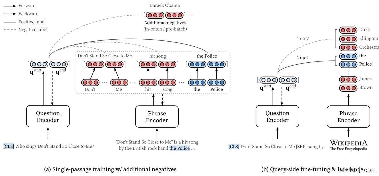
Figure 1: An overview of Dense Phrases. (a) We learn dense phrase representations in a single passage (§4.1) along with in-batch and pre-batch negatives $(\S4.2,\S4.3)$ . (b) With the top $k$ retrieved phrase representations from the entire text corpus (§5), we further perform query-side fine-tuning to optimize the question encoder (§6). During inference, our model simply returns the top-1 prediction.
图 1: Dense Phrases 概述。(a) 我们在单个段落中学习密集短语表示 (§4.1) 以及批次内和预批次负样本 $(\S4.2,\S4.3)$。(b) 通过从整个文本语料库中检索到的前 $k$ 个短语表示 (§5),我们进一步执行查询端微调以优化问题编码器 (§6)。在推理阶段,我们的模型仅返回 top-1 预测结果。
$$
E_{q}(q)=[\mathbf{q}^{\mathrm{start}},\mathbf{q}^{\mathrm{end}}]\in\mathbb{R}^{2d}.
$$
$$
E_{q}(q)=[\mathbf{q}^{\mathrm{start}},\mathbf{q}^{\mathrm{end}}]\in\mathbb{R}^{2d}.
$$
Note that we use pre-trained language models to initialize $\mathcal{M}{p}$ , $\mathcal{M}{q,\mathrm{start}}$ and $\mathcal{M}{q,\mathrm{end}}$ and they are fine-tuned with the objectives that we will define later. In our pilot experiments, we found that SpanBERT (Joshi et al., 2020) leads to superior performance compared to BERT (Devlin et al., 2019). SpanBERT is designed to predict the information in the entire span from its two endpoints, therefore it is well suited for our phrase representations. In our final model, we use SpanBERT-base-cased as our base LMs for $E_{s}$ and $E_{q}$ , and hence $d=768.$ .5 See Table 5 for an ablation study.
需要注意的是,我们使用预训练语言模型来初始化 $\mathcal{M}{p}$、$\mathcal{M}{q,\mathrm{start}}$ 和 $\mathcal{M}{q,\mathrm{end}}$,并通过后续定义的目标进行微调。在初步实验中,我们发现 SpanBERT (Joshi et al., 2020) 相比 BERT (Devlin et al., 2019) 能带来更优性能。SpanBERT 的设计初衷是通过两端点预测整个片段的信息,因此非常适合我们的短语表示任务。最终模型中,我们采用 SpanBERT-base-cased 作为 $E_{s}$ 和 $E_{q}$ 的基础大语言模型,故 $d=768$。消融实验详见表 5。
4 Learning Phrase Representations
4 学习短语表示
In this section, we start by learning dense phrase representations from the supervision of reading comprehension tasks, i.e., a single passage $p$ contains an answer $a^{*}$ to a question $q$ . Our goal is to learn strong dense representations of phrases for $s\in S(p)$ , which can be retrieved by a dense represent ation of the question and serve as a direct answer (§4.1). Then, we introduce two different negative sampling methods $(\S4.2,\S4.3)$ , which encourage the phrase representations to be better discriminated at the full Wikipedia scale. See Figure 1 for an overview of Dense Phrases.
在本节中,我们首先从阅读理解任务的监督中学习密集短语表示,即单个段落 $p$ 包含问题 $q$ 的答案 $a^{*}$。我们的目标是学习 $s\in S(p)$ 的强密集短语表示,这些表示可以通过问题的密集表示进行检索并作为直接答案(见4.1节)。接着,我们介绍了两种不同的负采样方法 $(\S4.2,\S4.3)$ ,这些方法促使短语表示在完整的维基百科规模上具有更好的区分能力。Dense Phrases的概述见图1。
4.1 Single-passage Training
4.1 单段落训练
To learn phrase representations in a single passage along with question representations, we first maximize the log-likelihood of the start and end positions of the gold phrase $s^{}$ where $\operatorname{TEXT}(s^{})=a^{*}$ . The training loss for predicting the start position of a phrase given a question is computed as:
为了在单段落中学习短语表征与问题表征,我们首先最大化黄金短语 $s^{}$ 起止位置的对数似然,其中 $\operatorname{TEXT}(s^{})=a^{*}$。给定问题时预测短语起始位置的训练损失计算如下:
$$
\begin{array}{r l}&{z_{1}^{\mathrm{start}},\dots,z_{m}^{\mathrm{start}}=[\mathbf{h}{1}^{\top}\mathbf{q}^{\mathrm{start}},\dots,\mathbf{h}{m}^{\top}\mathbf{q}^{\mathrm{start}}],}\ &{\qquadP^{\mathrm{start}}=\mathrm{softmax}(z_{1}^{\mathrm{start}},\dots,z_{m}^{\mathrm{start}}),}\ &{\qquad\mathcal{L}{\mathrm{start}}=-\log P_{\mathrm{start}}^{\mathrm{start}}(s^{*})^{.}}\end{array}
$$
$$
\begin{array}{r l}&{z_{1}^{\mathrm{start}},\dots,z_{m}^{\mathrm{start}}=[\mathbf{h}{1}^{\top}\mathbf{q}^{\mathrm{start}},\dots,\mathbf{h}{m}^{\top}\mathbf{q}^{\mathrm{start}}],}\ &{\qquadP^{\mathrm{start}}=\mathrm{softmax}(z_{1}^{\mathrm{start}},\dots,z_{m}^{\mathrm{start}}),}\ &{\qquad\mathcal{L}{\mathrm{start}}=-\log P_{\mathrm{start}}^{\mathrm{start}}(s^{*})^{.}}\end{array}
$$
We can define $\mathcal{L}_{\mathrm{end}}$ in a similar way and the final loss for the single-passage training is
我们可以用类似的方式定义 $\mathcal{L}_{\mathrm{end}}$,单段落训练的最终损失为
$$
\mathcal{L}{\mathrm{single}}=\frac{\mathcal{L}{\mathrm{start}}+\mathcal{L}_{\mathrm{end}}}{2}.
$$
$$
\mathcal{L}{\mathrm{single}}=\frac{\mathcal{L}{\mathrm{start}}+\mathcal{L}_{\mathrm{end}}}{2}.
$$
This essentially learns reading comprehension without any cross-attention between the passage and the question tokens, which fully decomposes phrase and question representations.
这实质上是在没有任何篇章与问题token间交叉注意力的情况下学习阅读理解能力,从而完全分解了短语和问题的表征。
Data augmentation Since the contextual i zed word representations $\mathbf{h}{1},\ldots,\mathbf{h}{m}$ are encoded in a query-agnostic way, they are always inferior to query-dependent representations in cross-attention models (Devlin et al., 2019), where passages are fed along with the questions concatenated by a special token such as [SEP]. We hypothesize that one key reason for the performance gap is that reading comprehension datasets only provide a few annotated questions in each passage, compared to the set of possible answer phrases. Learning from this supervision is not easy to differentiate similar phrases in one passage (e.g., $s^{*}=$ Charles, Prince of Wales and another $s=P_{\mathrm{}}$ rince George for a question $q=$ Who is next in line to be the monarch of England?).
数据增强 由于上下文词表示 $\mathbf{h}{1},\ldots,\mathbf{h}{m}$ 是以查询无关(query-agnostic)方式编码的,它们在跨注意力模型中始终逊色于查询依赖(query-dependent)表示 (Devlin et al., 2019) 。在跨注意力模型中,文章会与通过特殊token(如[SEP])拼接的问题一起输入。我们假设性能差距的一个关键原因是:与可能的答案短语集合相比,阅读理解数据集通常只在每篇文章中提供少量标注问题。从这种监督信号中学习难以区分文章中相似的短语(例如对于问题 $q=$ 谁是英国王位的第一顺位继承人? ,存在 $s^{*}=$ 查尔斯王子和另一个 $s=P_{\mathrm{}}$ 乔治王子这样的情况)。
Following this intuition, we propose to use a simple model to generate additional questions for data augmentation, based on a T5-large model (Raffel et al., 2020). To train the question genera- tion model, we feed a passage $p$ with the gold answer $s^{*}$ highlighted by inserting surrounding special tags. Then, the model is trained to maximize the log-likelihood of the question words of $q$ . After training, we extract all the named entities in each training passage as candidate answers and feed the passage $p$ with each candidate answer to generate questions. We keep the questionanswer pairs only when a cross-attention reading comprehension model6 makes a correct prediction on the generated pair. The remaining generated QA pairs ${(\bar{q}{1},\bar{s}{1}),(\bar{q}{2},\bar{s}{2}),\ldots,(\bar{q}{r},\bar{s}_{r})}$ are directly augmented to the original training set.
基于这一思路,我们提出使用一个简单模型来生成额外问题以进行数据增强,该模型基于T5-large (Raffel et al., 2020)。训练问题生成模型时,我们将带有黄金答案 $s^{*}$ 的文本段落 $p$ 通过插入特殊标记进行高亮处理后输入模型。随后,模型通过最大化问题 $q$ 的词对数似然进行训练。训练完成后,我们从每个训练段落中提取所有命名实体作为候选答案,并将段落 $p$ 与每个候选答案组合输入模型来生成问题。仅当交叉注意力阅读理解模型6对生成的问题-答案对做出正确预测时,我们才保留该问答对。最终保留的生成问答对 ${(\bar{q}{1},\bar{s}{1}),(\bar{q}{2},\bar{s}{2}),\ldots,(\bar{q}{r},\bar{s}_{r})}$ 会直接扩充至原始训练集。
Distillation We also propose improving the phrase representations by distilling knowledge from a cross-attention model (Hinton et al., 2015). We minimize the Kullback–Leibler divergence between the probability distribution from our phrase encoder and that from a standard SpanBERT-base QA model. The loss is computed as follows:
蒸馏
我们还提出通过从交叉注意力模型 (Hinton et al., 2015) 中蒸馏知识来改进短语表示。我们最小化短语编码器的概率分布与标准 SpanBERT-base QA 模型概率分布之间的 Kullback-Leibler 散度。损失计算如下:
$$
\mathcal{L}{\mathrm{distill}}=\frac{\mathrm{KL}(P^{\mathrm{start}}||P_{c}^{\mathrm{start}})+\mathrm{KL}(P^{\mathrm{end}}||P_{c}^{\mathrm{end}})}{2},
$$
$$
\mathcal{L}{\mathrm{distill}}=\frac{\mathrm{KL}(P^{\mathrm{start}}||P_{c}^{\mathrm{start}})+\mathrm{KL}(P^{\mathrm{end}}||P_{c}^{\mathrm{end}})}{2},
$$
where $P^{\mathrm{start}}$ (and $P^{\mathrm{end}}$ ) is defined in Eq. (5) and $P_{c}^{\mathrm{start}}$ and $P_{c}^{\mathrm{end}}$ denote the probability distributions used to predict the start and end positions of answers in the cross-attention model.
其中 $P^{\mathrm{start}}$ (及 $P^{\mathrm{end}}$ ) 由式 (5) 定义,$P_{c}^{\mathrm{start}}$ 和 $P_{c}^{\mathrm{end}}$ 表示交叉注意力模型中用于预测答案起止位置的概率分布。
4.2 In-batch Negatives
4.2 批次内负样本 (In-batch Negatives)
Eventually, we need to build phrase representations for billions of phrases. Therefore, a bigger challenge is to incorporate more phrases as negatives so the representations can be better discriminated at a larger scale. While Seo et al. (2019) simply sample two negative passages based on question similarity, we use in-batch negatives for our dense phrase representations, which has been shown to be effective in learning dense passage representations before (Karpukhin et al., 2020).
最终,我们需要为数十亿个短语构建表征。因此,更大的挑战在于引入更多短语作为负样本,以便在更大规模上更好地区分这些表征。虽然 Seo 等人 (2019) 仅基于问题相似度采样两个负段落,但我们采用批次内负样本 (in-batch negatives) 来优化密集短语表征,该方法此前已被证明能有效学习密集段落表征 (Karpukhin 等人, 2020)。

Figure 2: Two types of negative samples for the first batch item $(\mathbf{q}_{1}^{\mathrm{start}})$ in a mini-batch of size $B=4$ and $C=3$ . Note that the negative samples for the end representations $(\mathbf{q}_{i}^{\mathrm{end}})$ are obtained in a similar manner. See $\S4.2$ and $\S4.3$ for more details.
图 2: 在批次大小 $B=4$ 和 $C=3$ 的小批次中,针对第一个批次项 $(\mathbf{q}_{1}^{\mathrm{start}})$ 的两种负样本类型。注意,结束表示 $(\mathbf{q}_{i}^{\mathrm{end}})$ 的负样本以类似方式获得。更多细节请参阅 $\S4.2$ 和 $\S4.3$。
As shown in Figure 2 (a), for the $i$ -th example in a mini-batch of size $B$ , we denote the hidden representations of the gold start and end positions $\mathbf{h}{\mathit{s t a r t}}(s^{})$ and $\mathbf{h}{\mathrm{end}(s^{*})}$ as $\mathbf{g}{i}^{\mathrm{start}}$ and $\mathbf{g}{i}^{\mathrm{end}}$ , as well as the question representation as $[\mathbf{q}{i}^{\mathrm{start}},\mathbf{q}{i}^{\mathrm{end}}]$ . Let ${\bf G}^{\mathrm{start}},{\bf G}^{\mathrm{end}},{\bf Q}^{\mathrm{start}},{\bf Q}^{\mathrm{end}}$ be the $B\times d$ matrices and each row corresponds to $\mathbf{g}{i}^{\mathrm{start}},\mathbf{g}{i}^{\mathrm{end}},\mathbf{q}{i}^{\mathrm{start}},\mathbf{q}{i}^{\mathrm{end}}$ respectively. Basically, we can treat all the gold phrases from other passages in the same mini-batch as negative examples. We compute $\mathbf{S}^{\mathrm{start}}=\mathbf{Q}^{\mathrm{start}}\mathbf{G}^{\mathrm{start}\intercal}$ and $\mathbf{S}^{\mathrm{end}}=$ $\mathbf{Q}^{\mathrm{end}}\mathbf{G}^{\mathrm{end}\top}$ and the $i$ -th row of $\mathbf{S}^{\mathrm{start}}$ and ${\bf S}^{\mathrm{end}}$ return $B$ scores each, including a positive score and $B{-}1$ negative scores: $s_{1}^{\mathrm{start}},\ldots,s_{B}^{\mathrm{start}}$ and sen d, $s_{1}^{\mathrm{end}},\ldots,s_{B}^{\mathrm{end}}$ Similar to Eq. (5), we can compute the loss function for the $i$ -th example as:
如图2(a)所示,对于大小为$B$的小批量中的第$i$个样本,我们将黄金起始和结束位置$\mathbf{h}{\mathit{start}}(s^{})$与$\mathbf{h}{\mathrm{end}(s^{*})}$的隐藏表示记为$\mathbf{g}{i}^{\mathrm{start}}$和$\mathbf{g}{i}^{\mathrm{end}}$,问题表示记为$[\mathbf{q}{i}^{\mathrm{start}},\mathbf{q}{i}^{\mathrm{end}}]$。设${\bf G}^{\mathrm{start}},{\bf G}^{\mathrm{end}},{\bf Q}^{\mathrm{start}},{\bf Q}^{\mathrm{end}}$为$B\times d$矩阵,每行分别对应$\mathbf{g}{i}^{\mathrm{start}},\mathbf{g}{i}^{\mathrm{end}},\mathbf{q}{i}^{\mathrm{start}},\mathbf{q}{i}^{\mathrm{end}}$。本质上,我们可以将同一小批量中其他段落的所有黄金短语视为负样本。计算$\mathbf{S}^{\mathrm{start}}=\mathbf{Q}^{\mathrm{start}}\mathbf{G}^{\mathrm{start}\intercal}$和$\mathbf{S}^{\mathrm{end}}=$ $\mathbf{Q}^{\mathrm{end}}\mathbf{G}^{\mathrm{end}\top}$,$\mathbf{S}^{\mathrm{start}}$和${\bf S}^{\mathrm{end}}$的第$i$行各返回$B$个分数,包括一个正分数和$B{-}1$个负分数:$s_{1}^{\mathrm{start}},\ldots,s_{B}^{\mathrm{start}}$与$s_{1}^{\mathrm{end}},\ldots,s_{B}^{\mathrm{end}}$。类似于公式(5),第$i$个样本的损失函数可计算为:
$$
\begin{array}{r l}&{P_{i}^{\mathrm{start_ib}}=\mathrm{softmax}(s_{1}^{\mathrm{start}},\dots,s_{B}^{\mathrm{start}}),}\ &{P_{i}^{\mathrm{end_ib}}=\mathrm{softmax}(s_{1}^{\mathrm{end}},\dots,s_{B}^{\mathrm{end}}),}\ &{\quad\quad\mathcal{L}{\mathrm{neg}}=-\frac{\log P_{i}^{\mathrm{start_ib}}+\log P_{i}^{\mathrm{end_ib}}}{2},}\end{array}
$$
$$
\begin{array}{r l}&{P_{i}^{\mathrm{start_ib}}=\mathrm{softmax}(s_{1}^{\mathrm{start}},\dots,s_{B}^{\mathrm{start}}),}\ &{P_{i}^{\mathrm{end_ib}}=\mathrm{softmax}(s_{1}^{\mathrm{end}},\dots,s_{B}^{\mathrm{end}}),}\ &{\quad\quad\mathcal{L}{\mathrm{neg}}=-\frac{\log P_{i}^{\mathrm{start_ib}}+\log P_{i}^{\mathrm{end_ib}}}{2},}\end{array}
$$
We also attempted using non-gold phrases from other passages as negatives but did not find a meaningful improvement.
我们还尝试使用其他段落中的非黄金短语作为负样本,但未发现明显改进。
4.3 Pre-batch Negatives
4.3 预批次负样本
The in-batch negatives usually benefit from a large batch size (Karpukhin et al., 2020). However, it is challenging to further increase batch sizes, as they are bounded by the size of GPU memory. Next, we propose a novel negative sampling method called pre-batch negatives, which can effectively utilize the representations from the preceding $C$ mini-batches (Figure 2 (b)). In each iteration, we maintain a FIFO queue of $C$ mini-batches to cache phrase representations $\mathbf{G}^{\mathrm{start}}$ and $\mathbf{G}^{\mathrm{end}}$ . The cached phrase representations are then used as negative samples for the next iteration, providing $B\times C$ additional negative samples in total.7
批次内负样本通常受益于较大的批次大小 (Karpukhin et al., 2020)。然而,由于受限于GPU内存容量,进一步增大批次大小具有挑战性。为此,我们提出了一种名为批次前负样本的新型负采样方法,该方法能有效利用前$C$个小批次的表征 (图2(b))。在每次迭代中,我们维护一个包含$C$个小批次的FIFO队列,用于缓存短语表征$\mathbf{G}^{\mathrm{start}}$和$\mathbf{G}^{\mathrm{end}}$。这些缓存的短语表征将作为下一次迭代的负样本,共计提供$B\times C$个额外负样本。
These pre-batch negatives are used together with in-batch negatives and the training loss is the same as Eq. (8), except that the gradients are not backpropagated to the cached pre-batch negatives. After warming up the model with in-batch negatives, we simply shift from in-batch negatives $(B-1$ negatives) to in-batch and pre-batch negatives (hence a total number of $B\times C+B-1$ negatives). For simplicity, we use $\mathcal{L}_{\mathrm{neg}}$ to denote the loss for both inbatch negatives and pre-batch negatives. Since we do not retain the computational graph for pre-batch negatives, the memory consumption of pre-batch negatives is much more manageable while allowing an increase in the number of negative samples.
这些预批次负样本与批次内负样本共同使用,训练损失与公式(8)相同,只是梯度不会反向传播到缓存的预批次负样本。在用批次内负样本预热模型后,我们只需从批次内负样本($B-1$个负样本)切换到批次内和预批次负样本(因此总负样本数为$B\times C+B-1$个)。为简洁起见,我们用$\mathcal{L}_{\mathrm{neg}}$表示批次内负样本和预批次负样本的损失。由于我们不为预批次负样本保留计算图,预批次负样本的内存消耗更易管理,同时允许增加负样本数量。
4.4 Training Objective
4.4 训练目标
Finally, we optimize all the three losses together, on both annotated reading comprehension examples and generated questions from $\S4.1$ :
最后,我们在标注的阅读理解示例和从$\S4.1$生成的问题上共同优化所有三个损失函数:
$$
\mathcal{L}=\lambda_{1}\mathcal{L}{\mathrm{single}}+\lambda_{2}\mathcal{L}{\mathrm{distill}}+\lambda_{3}\mathcal{L}_{\mathrm{neg}},
$$
$$
\mathcal{L}=\lambda_{1}\mathcal{L}{\mathrm{single}}+\lambda_{2}\mathcal{L}{\mathrm{distill}}+\lambda_{3}\mathcal{L}_{\mathrm{neg}},
$$
where $\lambda_{1},\lambda_{2},\lambda_{3}$ determine the importance of each loss term. We found that $\lambda_{1}=1$ , $\lambda_{2}=2$ , and $\lambda_{3}=$ 4 works well in practice. See Table 5 and Table 6 for an ablation study of different components.
其中 $\lambda_{1},\lambda_{2},\lambda_{3}$ 决定各项损失的权重。实践发现 $\lambda_{1}=1$、$\lambda_{2}=2$ 和 $\lambda_{3}=4$ 效果最佳。不同组件的消融实验详见表5和表6。
5 Indexing and Search
5 索引与搜索
Indexing After training the phrase encoder $E_{s}$ , we need to encode all the phrases $S({\mathcal{D}})$ in the entire English Wikipedia $\mathcal{D}$ and store an index of the phrase dump. We segment each document $d_{i} \in~\mathcal{D}$ into a set of natural paragraphs, from which we obtain token representations for each paragraph using $E_{s}(\cdot)$ . Then, we build a phrase dump $\mathbf{H}=[\mathbf{h}{1},\dots,\mathbf{h}{|\mathcal{W}(\mathcal{D})|}]\in\mathbb{R}^{|\mathcal{W}(\mathcal{D})|\times d}$ by stacking the token representations from all the paragraphs in $\mathcal{D}$ . Note that this process is computationally expensive and takes about hundreds of GPU hours with a large disk footprint. To reduce the size of phrase dump, we follow and modify several techniques introduced in Seo et al. (2019) (see Appendix E for details). After indexing, we can use two rows $i$ and $j$ of $\mathbf{H}$ to represent a dense phrase representation $[\mathbf{h}{i},\mathbf{h}_{j}]$ . We use faiss (Johnson et al., 2017) for building a MIPS index of $\mathbf{H}$ .8
索引构建
训练完短语编码器 $E_{s}$ 后,我们需要对整个英文维基百科 $\mathcal{D}$ 中的所有短语 $S({\mathcal{D}})$ 进行编码,并存储短语库的索引。我们将每篇文档 $d_{i} \in~\mathcal{D}$ 分割为若干自然段落,并使用 $E_{s}(\cdot)$ 获取每个段落的token表征。接着,通过堆叠 $\mathcal{D}$ 中所有段落的token表征,构建短语库 $\mathbf{H}=[\mathbf{h}{1},\dots,\mathbf{h}{|\mathcal{W}(\mathcal{D})|}]\in\mathbb{R}^{|\mathcal{W}(\mathcal{D})|\times d}$。需要注意的是,该过程计算开销极大,需消耗数百GPU小时且占用大量磁盘空间。为缩减短语库体积,我们采用并改进了Seo等人 (2019) 提出的若干技术(详见附录E)。索引构建完成后,可用 $\mathbf{H}$ 的第 $i$ 行和第 $j$ 行表示稠密短语表征 $[\mathbf{h}{i},\mathbf{h}_{j}]$。我们使用faiss (Johnson等人, 2017) 为 $\mathbf{H}$ 建立MIPS索引。8
Search For a given question $q$ , we can find the answer $\hat{s}$ as follows:
对于给定问题 $q$,我们可以通过以下方式找到答案 $\hat{s}$:
$$
\begin{array}{r l}&{\boldsymbol{\hat{s}}=\underset{\boldsymbol{s}{(i,j)}}{\operatorname{argmax}}E_{s}(\boldsymbol{s}{(i,j)},\mathcal{D})^{\top}E_{q}(\boldsymbol{q}),}\ &{\quad=\underset{\boldsymbol{s}{(i,j)}}{\operatorname{argmax}}(\mathbf{Hq}^{\operatorname{start}}){i}+(\mathbf{Hq}^{\operatorname{end}})_{j},}\end{array}
$$
$$
\begin{array}{r l}&{\boldsymbol{\hat{s}}=\underset{\boldsymbol{s}{(i,j)}}{\operatorname{argmax}}E_{s}(\boldsymbol{s}{(i,j)},\mathcal{D})^{\top}E_{q}(\boldsymbol{q}),}\ &{\quad=\underset{\boldsymbol{s}{(i,j)}}{\operatorname{argmax}}(\mathbf{Hq}^{\operatorname{start}}){i}+(\mathbf{Hq}^{\operatorname{end}})_{j},}\end{array}
$$
where $s_{(i,j)}$ denotes a phrase with start and end indices as $i$ and $j$ in the index $\mathbf{H}$ . We can compute the argmax of $\mathbf{Hq}^{\mathrm{start}}$ and $\mathbf{Hq}^{\mathrm{end}}$ efficiently by performing MIPS over $\mathbf{H}$ with $\mathbf{q}^{\mathrm{start}}$ and $\mathbf{q}^{\mathrm{end}}$ . In practice, we search for the top $k$ start and top $k$ end positions separately and perform a constrained search over their end and start positions respectively such that $1\leq i\leq j<i+L\leq|\mathcal{W}(\mathcal{D})|$ .
其中 $s_{(i,j)}$ 表示在索引 $\mathbf{H}$ 中起止位置为 $i$ 和 $j$ 的短语。我们可以通过用 $\mathbf{q}^{\mathrm{start}}$ 和 $\mathbf{q}^{\mathrm{end}}$ 对 $\mathbf{H}$ 执行最大内积搜索 (MIPS) 来高效计算 $\mathbf{Hq}^{\mathrm{start}}$ 和 $\mathbf{Hq}^{\mathrm{end}}$ 的 argmax。实际应用中,我们分别搜索前 $k$ 个起始位置和前 $k$ 个结束位置,并在满足 $1\leq i\leq j<i+L\leq|\mathcal{W}(\mathcal{D})|$ 的条件下对它们的起止位置进行约束搜索。
6 Query-side Fine-tuning
6 查询端微调
So far, we have created a phrase dump $\mathbf{H}$ that supports efficient MIPS search. In this section, we propose a novel method called query-side fine-tuning by only updating the question encoder $E_{q}$ to correctly retrieve a desired answer $a^{}$ for a question $q$ given $\mathbf{H}$ . Formally speaking, we optimize the marginal log-likelihood of the gold answer $a^{*}$ for a question $q$ , which resembles the weakly-supervised QA setting in previous work (Lee et al., 2019; Min et al., 2019). For every question $q$ , we retrieve top $k$ phrases and minimize the objective:
目前,我们已构建了一个支持高效MIPS搜索的短语库$\mathbf{H}$。本节提出一种称为查询端微调的新方法,仅通过更新问题编码器$E_{q}$,实现在给定$\mathbf{H}$时准确检索问题$q$对应的目标答案$a^{}$。形式化地,我们优化问题$q$对应黄金答案$a^{*}$的边际对数似然,这与前人工作中的弱监督QA设定类似 (Lee et al., 2019; Min et al., 2019)。对于每个问题$q$,我们检索top $k$个短语并最小化目标函数:
$$
\begin{array}{r}{\mathcal{L}{\mathrm{query}}=-\log\frac{\sum_{s\in\tilde{S}(q),\mathrm{TEXT}(s)=a^{*}}\exp\big(f(s|\mathcal{D},q)\big)}{\sum_{s\in\tilde{S}(q)}\exp\big(f(s|\mathcal{D},q)\big)},}\end{array}
$$
$$
\begin{array}{r}{\mathcal{L}{\mathrm{query}}=-\log\frac{\sum_{s\in\tilde{S}(q),\mathrm{TEXT}(s)=a^{*}}\exp\big(f(s|\mathcal{D},q)\big)}{\sum_{s\in\tilde{S}(q)}\exp\big(f(s|\mathcal{D},q)\big)},}\end{array}
$$
where $f(s|\mathcal{D},q)$ is the score of the phrase $s$ (Eq. (2)) and $\tilde{\cal S}(q)$ denotes the top $k$ phrases for $q$ (Eq. (10)). In practice, we use $k=100$ for all the experiments.
其中 $f(s|\mathcal{D},q)$ 表示短语 $s$ 的得分(公式(2)),$\tilde{\cal S}(q)$ 表示查询 $q$ 的前 $k$ 个短语(公式(10))。实际实验中,我们统一采用 $k=100$ 作为参数设置。
There are several advantages for doing this: (1) we find that query-side fine-tuning can reduce the discrepancy between training and inference, and hence improve the final performance substantially (§8). Even with effective negative sampling, the model only sees a small portion of passages compared to the full scale of $\mathcal{D}$ and this training objective can effectively fill in the gap. (2) This training strategy allows for transfer learning to unseen domains, without rebuilding the entire phrase index. More specifically, the model is able to quickly adapt to new QA tasks (e.g., Web Questions) when the phrase dump is built using SQuAD or Natural Questions. We also find that this can transfers to non-QA tasks when the query is written in a different format. In $\S7.3$ , we show the possibility of directly using Dense Phrases for slot filling tasks by using a query such as (Michael Jackson, is a singer of, $x_{.}$ ). In this regard, we can view our model as a dense knowledge base that can be accessed by many different types of queries and it is able to return phrase-level knowledge efficiently.
这样做有几个优势:(1) 我们发现查询端微调可以减少训练和推理之间的差异,从而显著提高最终性能(§8)。即使采用有效的负采样,与完整的$\mathcal{D}$规模相比,模型也只能看到一小部分段落,而这种训练目标可以有效填补这一空白。(2) 这种训练策略允许在不重建整个短语索引的情况下,将学习迁移到未见过的领域。更具体地说,当使用SQuAD或Natural Questions构建短语转储时,模型能够快速适应新的QA任务(例如Web Questions)。我们还发现,当查询以不同格式编写时,这种方法也可以迁移到非QA任务。在$\S7.3$中,我们展示了通过使用诸如(Michael Jackson, is a singer of, $x_{.}$)这样的查询,直接使用Dense Phrases进行槽填充任务的可能性。在这方面,我们可以将我们的模型视为一个密集的知识库,可以通过许多不同类型的查询进行访问,并且能够高效地返回短语级别的知识。
7 Experiments
7 实验
7.1Setup
7.1 设置
Datasets. We use two reading comprehension datasets: SQuAD (Rajpurkar et al., 2016) and Natural Questions (NQ) (Kwiatkowski et al., 2019) to learn phrase representations, in which a single gold passage is provided for each question. For the opendomain QA experiments, we evaluate our approach on five popular open-domain QA datasets: Natural Questions, Web Questions (WQ) (Berant et al., 2013), Curate dT REC (TREC) (Baudis and Sedivy, 2015), TriviaQA (TQA) (Joshi et al., 2017), and SQuAD. Note that we only use SQuAD and/or NQ to build the phrase index and perform query-side fine-tuning (§6) for other datasets.
数据集。我们使用两个阅读理解数据集:SQuAD (Rajpurkar et al., 2016) 和 Natural Questions (NQ) (Kwiatkowski et al., 2019) 来学习短语表示,其中每个问题都提供了一个标准段落。对于开放域问答实验,我们在五个流行的开放域问答数据集上评估我们的方法:Natural Questions、Web Questions (WQ) (Berant et al., 2013)、Curated TREC (TREC) (Baudis and Sedivy, 2015)、TriviaQA (TQA) (Joshi et al., 2017) 和 SQuAD。请注意,我们仅使用 SQuAD 和/或 NQ 来构建短语索引并为其他数据集执行查询端微调 (§6)。
We also evaluate our model on two slot filling tasks, to show how to adapt our Dense Phrases for other knowledge-intensive NLP tasks. We focus on using two slot filling datasets from the KILT benchmark (Petroni et al., 2021): T-REx (Elsahar et al., 2018) and zero-shot relation extraction (Levy et al., 2017). Each query is provided in the form of “{subject entity} [SEP] {relation}" and the answer is the object entity. Appendix C provides the statistics of all the datasets.
我们还评估了模型在两个槽填充任务上的表现,以展示如何将Dense Phrases适配到其他知识密集型NLP任务中。我们重点使用了来自KILT基准测试 (Petroni et al., 2021) 的两个槽填充数据集:T-REx (Elsahar et al., 2018) 和零样本关系抽取 (Levy et al., 2017)。每个查询以"{主体实体} [SEP] {关系}"的形式提供,答案为目标实体。附录C提供了所有数据集的统计信息。
Implementation details. We denote the training datasets used for reading comprehension (Eq. (9)) as $\mathcal{C}{\mathrm{phrase}}$ . For open-domain QA, we train two versions of phrase encoders, each of which are trained on $\ensuremath{\mathcal{C}}{\mathrm{phrase}} =~{\mathrm{SQuAD}}$ and ${\mathrm{NQ},\mathrm{SQuAD}}$ , respectively. We build the phrase dump H for the 2018-12-20 Wikipedia snapshot and perform queryside fine-tuning on each dataset using Eq. (11). For slot filling, we use the same phrase dump for opendomain QA, $\mathcal{C}_{\mathrm{phrase}}={\mathrm{NQ},\mathrm{SQuAD}}$ and perform query-side fine-tuning on randomly sampled 5K or 10K training examples to see how rapidly our model adapts to the new query types. See Appendix D for details on the hyper parameters and Appendix A for an analysis of computational cost.
实现细节。我们将用于阅读理解 (Eq. (9)) 的训练数据集记为 $\mathcal{C}{\mathrm{phrase}}$。对于开放域问答任务,我们训练了两个版本的短语编码器,分别基于 $\ensuremath{\mathcal{C}}{\mathrm{phrase}} =~{\mathrm{SQuAD}}$ 和 ${\mathrm{NQ},\mathrm{SQuAD}}$ 进行训练。基于 2018-12-20 版本的维基百科快照构建短语库 H,并使用 Eq. (11) 在每个数据集上进行查询侧微调。对于槽填充任务,我们使用与开放域问答相同的短语库 $\mathcal{C}_{\mathrm{phrase}}={\mathrm{NQ},\mathrm{SQuAD}}$,并在随机采样的 5K 或 10K 训练样本上进行查询侧微调,以观察模型适应新查询类型的速度。超参数细节参见附录 D,计算成本分析参见附录 A。
Table 2: Reading comprehension results, evaluated on the development sets of SQuAD and Natural Questions. Underlined numbers are estimated from the figures from the original papers. †: BERT-large model.
表 2: 阅读理解结果,在SQuAD和Natural Questions开发集上的评估结果。带下划线的数字是根据原始论文图表估算得出。†: BERT-large模型。
| 模型 | SQuAD | NQ (Long) |
|---|---|---|
| EM | F1 | |
| Query-Dependent | ||
| BERT-base | 80.8 | 88.5 |
| SpanBERT-base | 85.7 | 92.2 |
| Query-Agnostic | ||
| DilBERT (Siblini et al., 2020) | 63.0 | 72.0 |
| DeFormer (Ca0 et al., 2020) | 72.1 | |
| DenSPIt | 73.6 | 81.7 |
| DenSPI+ Sparc | 76.4 | 84.8 |
| DensePhrases (ours) | 78.3 | 86.3 |
7.2 Experiments: Question Answering
7.2 实验:问答任务
Reading comprehension. In order to show the effectiveness of our phrase representations, we first evaluate our model in the reading comprehension setting for SQuAD and NQ and report its performance with other query-agnostic models (Eq. (9) without query-side fine-tuning). This problem was originally formulated by Seo et al. (2018) as the phrase-indexed question answering (PIQA) task.
阅读理解。为了展示我们短语表示的有效性,我们首先在SQuAD和NQ的阅读理解场景中评估模型性能,并与其他查询无关模型(即未进行查询端微调的公式(9)模型)进行对比。该问题最初由Seo等人(2018)提出,被定义为短语索引问答(PIQA)任务。
Compared to previous query-agnostic models, our model achieves the best performance of 78.3 EM on SQuAD by improving the previous phrase retrieval model (DenSPI) by $4.7%$ (Table 2). Al- though it is still behind cross-attention models, the gap has been greatly reduced and serves as a strong starting point for the open-domain QA model.
与之前的查询无关模型相比,我们的模型通过将短语检索模型 (DenSPI) 提升 4.7% (表 2) ,在 SQuAD 上实现了 78.3 EM 的最佳性能。虽然仍落后于交叉注意力模型,但差距已大幅缩小,为开放域问答模型提供了坚实的基础起点。
Open-domain QA. Experimental results on open-domain QA are summarized in Table 3. Without any sparse representations, Dense Phrases outperforms previous phrase retrieval models by a large margin and achieves a $15%{-25%}$ absolute improvement on all datasets except SQuAD. Training the model of Lee et al. (2020) on $\mathcal{C}_{\mathrm{phrase}}=$ ${\mathrm{NQ},\mathrm{SQuAD}}$ only increases the result from $14.5%$ to $16.5%$ on NQ, demonstrating that it does not suffice to simply add more datasets for training phrase representations. Our performance is also competitive with recent retriever-reader models (Karpukhin et al., 2020), while running much faster during inference (Table 1).
开放域问答。开放域问答的实验结果总结在表 3 中。在不使用任何稀疏表示的情况下,Dense Phrases 大幅优于之前的短语检索模型,除 SQuAD 外,在所有数据集上实现了 $15%{-25%}$ 的绝对提升。在 $\mathcal{C}_{\mathrm{phrase}}={\mathrm{NQ},\mathrm{SQuAD}}$ 上训练 Lee 等人 (2020) 的模型仅将 NQ 的结果从 $14.5%$ 提高到 $16.5%$,这表明仅增加更多训练数据集不足以提升短语表示效果。我们的性能也与最近的检索器-阅读器模型 (Karpukhin 等人,2020) 相当,同时在推理时运行速度更快 (表 1)。
Table 3: Open-domain QA results. We report exact match (EM) on the test sets. We also show the additional training or pre-training datasets for learning the retriever models $(\mathcal{C}{\mathrm{retr}})$ and creating the phrase dump $(\mathcal{C}{\mathrm{phrase}})$ . ∗: no supervision using target training data (zero-shot). †: unlabeled data used for extra pre-training.
表 3: 开放域问答结果。我们报告了测试集上的精确匹配 (EM) 分数,并列出了用于训练检索器模型 $(\mathcal{C}{\mathrm{retr}})$ 和构建短语库 $(\mathcal{C}{\mathrm{phrase}})$ 的额外训练或预训练数据集。*: 未使用目标训练数据进行监督 (零样本)。†: 用于额外预训练的无标注数据。
| 模型 | NQ | WQ | TREC | TQA | SQuAD | |
|---|---|---|---|---|---|---|
| 检索器-阅读器 | Cretr: (预)训练 | |||||
| DrQA (Chen et al., 2017) | 20.7 | 25.4 | 29.8 | |||
| BERT+BM25 (Lee et al., 2019) | 26.5 | 17.7 | 21.3 | 47.1 | 33.2 | |
| ORQA (Lee et al., 2019) | {Wiki.}† | 33.3 | 36.4 | 30.1 | 45.0 | 20.2 |
| REALMNews (Guu et al., 2020) | {Wiki., CC-News} | 40.4 | 40.7 | 42.9 | ||
| DPR-multi (Karpukhin et al., 2020) | {NQ, WQ, TREC, TQA} | 41.5 | 42.4 | 49.4 | 56.8 | 24.1 |
| 短语检索 | Cphrase: 训练 | |||||
| DenSPI (Seo et al., 2019) | {SQuAD} | 8.1* | 11.1* | 31.6* | 30.7* | 36.2 |
| DenSPI + Sparc (Lee et al., 2020) | {SQuAD} | 14.5* | 17.3* | 35.7* | 34.4* | 40.7 |
| DenSPI + Sparc (Lee et al., 2020) | {NQ, SQuAD} | 16.5 | ||||
| DensePhrases (ours) | {SQuAD} | 31.2 | 36.3 | 50.3 | 53.6 | 39.4 |
| DensePhrases (ours) | {NQ, SQuAD} | 40.9 | 37.5 | 51.0 | 50.7 | 38.0 |
| 模型 | T-REx Acc | T-REx F1 | ZsRE Acc | ZsRE F1 |
|---|---|---|---|---|
| DPR+BERT | 4.47 | 27.09 | ||
| DPR+BART RAG | 11.12 | 11.41 | 18.91 | 20.32 |
| 23.12 | 23.94 | 36.83 | 39.91 | |
| DensePhrases5K | 25.32 | 29.76 | 40.39 | 45.89 |
| DensePhrases 10K | 27.84 | 32.34 | 41.34 | 46.79 |
Table 4: Slot filling results on the test sets of T-REx and Zero shot RE (ZsRE) in the KILT benchmark. We report KILT-AC and KILT-F1 (denoted as Acc and $F I$ in the table), which consider both span-level accuracy and correct retrieval of evidence documents.
表 4: KILT基准测试中T-REx和零样本关系抽取(ZsRE)测试集的槽填充结果。我们报告了KILT-AC和KILT-F1(表中记为Acc和$F I$),这两个指标同时考虑了片段级准确率和证据文档的正确检索。
7.3 Experiments: Slot Filling
7.3 实验:槽填充
Table 4 summarizes the results on the two slot filling datasets, along with the baseline scores provided by Petroni et al. (2021). The only extractive baseline is $\mathrm{DPR}+\mathrm{BERT}$ , which performs poorly in zero-shot relation extraction. On the other hand, our model achieves competitive performance on all datasets and achieves state-of-the-art performance on two datasets using only 5K training examples.
表 4 总结了两个槽填充数据集的结果,以及 Petroni 等人 (2021) 提供的基线分数。唯一的抽取式基线是 $\mathrm{DPR}+\mathrm{BERT}$ ,它在零样本关系抽取中表现不佳。相比之下,我们的模型在所有数据集上都取得了有竞争力的性能,并且仅使用 5K 训练样本就在两个数据集上达到了最先进的性能。
8 Analysis
8 分析
Ablation of phrase representations. Table 5 shows the ablation result of our model on SQuAD. Upon our choice of architecture, augmenting training set with generated questions $(\mathbf{Q}\mathbf{G}=\mathbf{\check{\Gamma}})$ and performing distillation from cross-attention models $({\mathrm{Distill}}={\checkmark})$ improve performance up to $\mathbf{EM}=$ 78.3. We attempted adding the generated questions to the training of the SpanBERT-QA model but find a $0.3%$ improvement, which validates that data sparsity is a bottleneck for query-agnostic models.
短语表征的消融实验。表5展示了我们的模型在SQuAD数据集上的消融结果。在我们选择的架构基础上,通过使用生成的问题增强训练集$(\mathbf{Q}\mathbf{G}=\mathbf{\check{\Gamma}})$ 以及从交叉注意力模型进行知识蒸馏$({\mathrm{Distill}}={\checkmark})$,性能提升至$\mathbf{EM}=$78.3。我们尝试将生成的问题加入SpanBERT-QA模型的训练中,但仅观察到$0.3%$的提升,这验证了数据稀疏性是查询无关模型的主要瓶颈。
Table 5: Ablation of Dense Phrases on the development set of SQuAD. Bb: BERT-base, Sb: SpanBERT-base, Bl: BERT-large. Share: whether question and phrase encoders are shared or not. Split: whether the full hidden vectors are kept or split into start and end vectors. QG: question generation (§4.1). Distill: distillation (Eq.(7)). DenSPI (Seo et al., 2019) also included a coherency scalar and see their paper for more details.
表 5: SQuAD开发集上密集短语的消融实验。Bb: BERT-base, Sb: SpanBERT-base, Bl: BERT-large。Share: 问题和短语编码器是否共享。Split: 完整隐藏向量是否保留或拆分为起始和结束向量。QG: 问题生成(§4.1)。Distill: 蒸馏(Eq.(7))。DenSPI (Seo et al., 2019)还包含了一个连贯性标量,详情请参阅其论文。
| 模型 | M | Share | Split | QG Distill | EM | |
|---|---|---|---|---|---|---|
| DenSPI | Bb. | × | 70.2 | |||
| Sb. | 68.5 | |||||
| Bl. | × | 73.6 | ||||
| Dense | Bb. | × | × | × | 70.2 | |
| Phrases | Bb. | × | × | × | 71.9 | |
| Sb. | × | × | × | × | 73.2 | |
| Sb. | × | × | 76.3 | |||
| Sb. | × | 78.3 |
Effect of batch negatives. We further evaluate the effectiveness of various negative sampling methods introduced in $\S4.2$ and $\S4.3$ . Since it is computationally expensive to test each setting at the full Wikipedia scale, we use a smaller text corpus $\mathcal{D}_{\mathrm{small}}$ of all the gold passages in the development sets of Natural Questions, for the ablation study. Empirically, we find that results are generally well correlated when we gradually increase the size of $|\mathcal D|$ . As shown in Table 6, both in-batch and pre-batch negatives bring substantial improvements. While using a larger batch size $\mathit{\Theta}(B=84\$ ) is beneficial for in-batch negatives, the number of preceding batches in pre-batch negatives is optimal when $C=2$ . Surprisingly, the pre-batch negatives also improve the performance when .
批次负样本的影响。我们进一步评估了$\S4.2$和$\S4.3$中介绍的各种负采样方法的有效性。由于在完整维基百科规模上测试每个设置的计算成本很高,我们使用自然问题开发集中所有黄金段落组成的较小文本语料库$\mathcal{D}_{\mathrm{small}}$进行消融研究。经验表明,当我们逐步增加$|\mathcal D|$的规模时,结果通常具有良好的相关性。如表6所示,批次内负样本和前序批次负样本都带来了显著改进。虽然使用更大的批次规模$\mathit{\Theta}(B=84$)对批次内负样本有益,但前序批次负样本的最佳前序批次数为$C=2$。令人惊讶的是,当$\mathcal{D}={p}$时,前序批次负样本也能提升性能。
Table 6: Effect of in-batch negatives and pre-batch negatives on the development set of Natural Questions. $B$ : batch size. $C$ : number of preceding mini-batches used in pre-batch negatives. $\mathcal{D}_{\mathrm{small}}$ : all the gold passages in the development set of NQ. ${p}$ : single passage.
表 6: 批内负样本和预批负样本对Natural Questions开发集的影响。$B$: 批次大小。$C$: 预批负样本中使用的前置小批次数量。$\mathcal{D}_{\mathrm{small}}$: NQ开发集中的所有黄金段落。${p}$: 单一段落。
| 类型 | B | C D={p} | D = Dsmall |
|---|---|---|---|
| 无 | 48 | 70.4 | 35.3 |
| + 批内负样本 | 48 | 70.5 | 52.4 |
| 84 | 70.3 | 54.2 | |
| + 预批负样本 | 84 | 1 71.6 | 59.8 |
| 84 | 2 71.9 | 60.4 | |
| 84 4 | 71.2 | 59.8 |
Effect of query-side fine-tuning. We summarize the effect of query-side fine-tuning in Table 7. For the datasets that were not used for training the phrase encoders (TQA, WQ, TREC), we observe a $15%$ to $20%$ improvement after query-side finetuning. Even for the datasets that have been used (NQ, SQuAD), it leads to significant improvements (e.g., $32.6%{\rightarrow}40.9%$ on NQ for $\mathcal{C}_{\mathrm{phrase}}={\mathrm{NQ}})$ and it clearly demonstrates it can effectively reduce the discrepancy between training and inference.
查询侧微调的效果。我们将查询侧微调的效果总结在表7中。对于未用于训练短语编码器的数据集(TQA、WQ、TREC),我们观察到查询侧微调后有15%到20%的提升。即使对于已使用的数据集(NQ、SQuAD),它也能带来显著改进(例如,在NQ上从32.6%提升至40.9%,当$\mathcal{C}_{\mathrm{phrase}}={\mathrm{NQ}}$时),这清楚地表明它能有效减少训练与推理之间的差异。
9 Related Work
9 相关工作
Learning effective dense representations of words is a long-standing goal in NLP (Bengio et al., 2003; Collobert et al., 2011; Mikolov et al., 2013; Peters et al., 2018; Devlin et al., 2019). Beyond words, dense representations of many different granularities of text such as sentences (Le and Mikolov, 2014; Kiros et al., 2015) or documents (Yih et al., 2011) have been explored. While dense phrase represent at ions have been also studied for statistical machine translation (Cho et al., 2014) or syntactic parsing (Socher et al., 2010), our work focuses on learning dense phrase representations for QA and any other knowledge-intensive tasks where phrases can be easily retrieved by performing MIPS.
学习有效的词级稠密表示一直是自然语言处理(NLP)领域的长期目标 (Bengio et al., 2003; Collobert et al., 2011; Mikolov et al., 2013; Peters et al., 2018; Devlin et al., 2019)。除单词外,研究者还探索了不同文本粒度的稠密表示,如句子级 (Le and Mikolov, 2014; Kiros et al., 2015) 或文档级 (Yih et al., 2011)。虽然稠密短语表示在统计机器翻译 (Cho et al., 2014) 和句法分析 (Socher et al., 2010) 中已有研究,但我们的工作聚焦于为问答(QA)和其他知识密集型任务学习稠密短语表示,这些任务可通过最大内积搜索(MIPS)轻松检索短语。
This type of dense retrieval has been also studied for sentence and passage retrieval (Humeau et al., 2019; Karpukhin et al., 2020) (see Lin et al., 2020 for recent advances in dense retrieval). While Dense Phrases is explicitly designed to retrieve phrases that can be used as an answer to given queries, retrieving phrases also naturally entails retrieving larger units of text, provided the datastore maintains the mapping between each phrase and the sentence and passage in which it occurs.
这种密集检索方法同样被应用于句子和段落检索 (Humeau等人, 2019; Karpukhin等人, 2020) (关于密集检索的最新进展可参见Lin等人, 2020)。虽然Dense Phrases明确设计用于检索可作为给定查询答案的短语,但检索短语自然也需要检索更大的文本单元,前提是数据存储库维护了每个短语与其所在句子及段落之间的映射关系。
Table 7: Effect of query-side fine-tuning in Dense Phrases on each test set. We report EM of each model before $(\mathrm{QS}=X)$ and after $\boldsymbol{\mathrm{(QS=}\checkmark)}$ the query-side fine-tuning.
表 7: Dense Phrases 中查询端微调对各测试集的影响。我们报告了每个模型在查询端微调前 $(\mathrm{QS}=X)$ 和后 $\boldsymbol{\mathrm{(QS=}\checkmark)}$ 的 EM 分数。
| QS | NQ | WQ TREC | TQA | SQuAD |
|---|---|---|---|---|
| Cphrase = {SQuAD} | ||||
| × √ | 12.3 31.2 | 11.8 36.3 | 36.9 34.6 50.3 53.6 | 35.5 39.4 |
| Cphrase = {NQ} | ||||
| x | 32.6 | 21.1 | 32.3 32.4 | 20.7 |
| 40.9 | 37.1 | 49.7 49.2 | 25.7 | |
| Cphrase = {NQ, SQuAD} | ||||
| 28.9 | 18.9 | 34.9 31.9 | 33.2 | |
| 40.9 | 37.5 | 51.0 50.7 | 38.0 |
10 Conclusion
10 结论
In this study, we show that we can learn dense representations of phrases at the Wikipedia scale, which are readily retrievable for open-domain QA and other knowledge-intensive NLP tasks. We learn both phrase and question encoders from the supervision of reading comprehension tasks and introduce two batch-negative techniques to better discriminate phrases at scale. We also introduce query-side fine-tuning that adapts our model to different types of queries. We achieve strong performance on five popular open-domain QA datasets, while reducing the storage footprint and improving latency significantly. We also achieve strong performance on two slot filling datasets using only a small number of training examples, showing the possibility of utilizing our Dense Phrases as a knowledge base.
在本研究中,我们证明了可以在维基百科规模上学习短语的密集表示,这些表示可直接用于开放域问答和其他知识密集型NLP任务。我们从阅读理解任务的监督中学习短语和问题编码器,并引入两种批量负样本技术以更好地在大规模数据中区分短语。我们还提出了查询端微调方法,使模型能适配不同类型的查询。在五个主流开放域问答数据集上取得了强劲性能,同时显著降低了存储占用并提升了响应速度。仅用少量训练样本就在两个槽填充数据集上表现优异,这表明我们的密集短语技术具备作为知识库使用的潜力。
A Computational Cost
计算成本
We describe the resources and time spent during inference (Table 1 and A.1) and indexing (Table A.1). With our limited GPU resources (24GB $\times4)$ , it takes about 20 hours for indexing the entire phrase representations. We also largely reduced the storage from 1,547GB to 320GB by (1) removing sparse representations and (2) using our sharing and split strategy. See Appendix E for the details on the reduction of storage footprint and Appendix B for the specification of our server for the benchmark.
我们描述了推理 (表1和A.1) 和索引 (表A.1) 过程中消耗的资源与时间。在有限的GPU资源 (24GB $\times4$) 下,对整个短语表示进行索引大约需要20小时。通过 (1) 移除稀疏表示和 (2) 采用共享分割策略,我们将存储空间从1,547GB大幅压缩至320GB。存储占用的优化细节见附录E,基准测试服务器配置见附录B。
Table A.1: Complexity analysis of three open-domain QA models during indexing and inference. For inference, we also report the minimum requirement of RAM and GPU memory for running each model with GPU. For computing #Q/s for CPU, we do not use GPUs but load all models on the RAM.
表 A.1: 三种开放域问答模型在索引和推理阶段的复杂度分析。对于推理环节,我们还列出了各模型在GPU运行时的最低RAM和显存要求。计算CPU的#Q/s时,我们不使用GPU而是将所有模型加载到RAM中。
B Server Specifications for Benchmark
B 基准测试服务器规格
To compare the complexity of open-domain QA models, we install all models in Table 1 on the same server using their public open-source code. Our server has the following specifications:
为比较开放域问答模型的复杂度,我们在同一服务器上使用公开开源代码安装了表1中的所有模型。服务器配置如下:
Table B.2: Server specification for the benchmark
表 B.2: 基准测试服务器规格
| 硬件配置 |
|---|
| Intel Xeon CPU E5-2630 v4 @2.20GHz 128GB RAM |
| 12GB GPU (TITAN Xp) × 2 |
| 2TB 970 EVO Plus NVMe M.2 SSD × 1 |
Table C.3: Statistics of five open-domain QA datasets and two slot filling datasets. We follow the same splits in open-domain QA for the two reading comprehension datasets (SQuAD and Natural Questions).
表 C.3: 五个开放域问答数据集和两个槽填充数据集的统计信息。对于两个阅读理解数据集 (SQuAD 和 Natural Questions),我们遵循开放域问答相同的划分方式。
| 索引方式 | 资源 | 存储 | 时间 |
|---|---|---|---|
| DPR | 32GBGPU×8 | 76GB | 17h |
| DenSPI+Sparc | 24GBGPU×4 | 1,547GB | 85h |
| DensePhrases | 24GB GPU ×4 | 320GB | 20h |
| 推理方式 | RAM/GPU | 每秒查询数 (GPU, CPU) |
|---|---|---|
| DPR | 86GB/17GB | 0.9, 0.04 |
| DenSPI+Sparc | 27GB/2GB | 2.1, 1.7 |
| DensePhrases | 12GB/2GB | 20.6, 13.6 |
For DPR, due to its large memory consumption, we use a similar server with a 24GB GPU (TITAN RTX). For all models, we use 1,000 randomly sam- pled questions from the Natural Questions development set for the speed benchmark and measure #Q/sec. We set the batch size to 64 for all models except BERTSerini, ORQA and REALM, which do not allow a batch size of more than 1 in their open-source implementations. #Q/sec for DPR includes retrieving passages and running a reader model and the batch size for the reader model is set to 8 to fit in the 24GB GPU (retriever batch size is still 64). For other hyper parameters, we use the default settings of each model. We also exclude the time and the number of questions in the first five iterations for warming up each model. Note that despite our effort to match the environment of each model, their latency can be affected by various different settings in their implementations such as the choice of library (PyTorch vs. Tensorflow).
对于DPR,由于其内存消耗较大,我们使用配备24GB GPU (TITAN RTX) 的类似服务器。所有模型均采用自然问答开发集中随机采样的1,000个问题进行速度基准测试,并测量每秒处理问题数 (#Q/sec)。除BERTSerini、ORQA和REALM外,所有模型的批次大小均设为64——这三种模型在开源实现中不允许批次大小超过1。DPR的#Q/sec指标包含段落检索和阅读器模型运行时间,为适配24GB GPU,阅读器模型的批次大小设为8 (检索器批次大小仍保持64)。其他超参数均采用各模型的默认设置。我们还排除了前五次迭代的预热时间和问题数量。需要注意的是,尽管我们尽力匹配各模型运行环境,但其延迟仍可能受到实现中不同设置的影响 (例如PyTorch与Tensorflow的库选择差异)。
| 数据集 | 训练集 | 开发集 | 测试集 |
|---|---|---|---|
| NaturalQuestions | 79,168 | 8,757 | 3,610 |
| WebQuestions | 3,417 | 361 | 2,032 |
| CuratedTrec | 1,353 | 133 | 694 |
| TriviaQA | 78,785 | 8,837 | 11,313 |
| SQuAD | 78,713 | 8,886 | 10,570 |
| T-REx | 2,284,168 | 5,000 | 5,000 |
| Zero-ShotRE | 147,909 | 3,724 | 4,966 |
C Data Statistics and Pre-processing
C 数据统计与预处理
In Table C.3, we show the statistics of five opendomain QA datasets and two slot filling datasets. Pre-processed open-domain QA datasets are provided by Chen et al. (2017) except Natural Questions and TriviaQA. We use a version of Natural Questions and TriviaQA provided by Min et al. (2019); Lee et al. (2019), which are pre-processed for the open-domain QA setting. Slot filling datasets are provided by Petroni et al. (2021). We use two reading comprehension datasets (SQuAD and Natural Questions) for training our model on Eq. (9). For SQuAD, we use the original dataset provided by the authors (Rajpurkar et al., 2016). For Natural Questions (Kwiatkowski et al., 2019), we use the pre-processed version provided by Asai et al. (2020).9 We use the short answer as a ground truth answer $a^{*}$ and its long answer as a gold passage $p$ . We also match the gold passages in Natural Questions to the paragraphs in Wikipedia whenever possible. Since we want to check the performance changes of our model with the growing number of tokens, we follow the same split (train/dev/test) used in Natural Questions-Open for the reading comprehension setting as well. During the validation of our model and baseline models, we exclude samples whose answers lie in a list or a table from a Wikipedia article.
在表 C.3 中,我们展示了五个开放域问答数据集和两个槽填充数据集的统计信息。除 Natural Questions 和 TriviaQA 外,预处理后的开放域问答数据集由 Chen 等人 (2017) 提供。我们使用的 Natural Questions 和 TriviaQA 版本来自 Min 等人 (2019) 和 Lee 等人 (2019),这些数据集已针对开放域问答场景进行预处理。槽填充数据集由 Petroni 等人 (2021) 提供。我们使用两个阅读理解数据集 (SQuAD 和 Natural Questions) 来训练公式 (9) 中的模型。对于 SQuAD,我们使用作者 (Rajpurkar 等人, 2016) 提供的原始数据集。对于 Natural Questions (Kwiatkowski 等人, 2019),我们采用 Asai 等人 (2020) 提供的预处理版本。我们将简短答案作为真实答案 $a^{*}$,其详细答案作为黄金段落 $p$。我们还会尽可能将 Natural Questions 中的黄金段落与维基百科段落进行匹配。为了观察模型性能随 token 数量增加的变化,我们在阅读理解场景中也采用 Natural Questions-Open 使用的相同数据划分 (训练集/开发集/测试集)。在验证模型和基线模型时,我们排除了答案位于维基百科文章列表或表格中的样本。
D Hyper parameters
D 超参数
We use the Adam optimizer (Kingma and Ba, 2015) in all our experiments. For training our phrase and question encoders with Eq. (9), we use a learning rate of 3e-5 and the norm of the gradient is clipped at 1. We use a batch size of $B=84$ and train each model for 4 epochs for all datasets, where the loss of pre-batch negatives is applied in the last two epochs. We use SQuAD to train our QG model10 and use spaCy11 for extracting named entities in each training passage, which are used to generate questions. The number of generated questions is 327,302 and 1,126,354 for SQuAD and Natural Questions, respectively. The number of preceding batches $C$ is set to 2.
我们在所有实验中都使用 Adam 优化器 (Kingma and Ba, 2015)。在训练短语和问题编码器时(式 (9)),我们采用 3e-5 的学习率,并将梯度范数裁剪为 1。批量大小设为 $B=84$,所有数据集均训练 4 个周期,其中最后两个周期应用批次负样本损失。使用 SQuAD 训练 QG 模型 10,并借助 spaCy 11 从每个训练段落中提取命名实体以生成问题。SQuAD 和 Natural Questions 生成的问题数量分别为 327,302 和 1,126,354 个。前置批次数 $C$ 设置为 2。
For the query-side fine-tuning with Eq. (11), we use a learning rate of 3e-5 and the norm of the gradient is clipped at 1. We use a batch size of 12 and train each model for 10 epochs for all datasets. The top $k$ for the Eq. (11) is set to 100. While we use a single 24GB GPU (TITAN RTX) for training the phrase encoders with Eq. (9), query-side fine-tuning is relatively cheap and uses a single 12GB GPU (TITAN Xp). Using the development set, we select the best performing model (based on EM) for each dataset, which are then evaluated on each test set. Since SpanBERT only supports cased models, we also truecase the questions (Lita et al., 2003) that are originally provided in the lowercase (Natural Questions and Web Questions).
对于使用公式(11)进行的查询端微调,我们采用3e-5的学习率,并将梯度范数裁剪为1。所有数据集均使用12的批量大小,每个模型训练10个周期。公式(11)中的top $k$ 值设为100。虽然我们使用单块24GB显存GPU(TITAN RTX)配合公式(9)训练短语编码器,但查询端微调计算成本较低,仅需单块12GB显存GPU(TITAN Xp)。基于开发集的表现(以EM为指标),我们为每个数据集选择最优模型,随后在各测试集上进行评估。由于SpanBERT仅支持区分大小写模型,我们对原始小写形式的问题(Natural Questions和Web Questions)进行了真实大小写转换(Lita et al., 2003)。
E Reducing Storage Footprint
E 减少存储占用
As shown in Table 1, we have reduced the storage footprint from 1,547GB (Lee et al., 2020) to 320GB. We detail how we can reduce the storage footprint in addition to the several techniques introduced by Seo et al. (2019).
如表 1 所示,我们将存储占用从 1,547GB (Lee et al., 2020) 降低到了 320GB。除了 Seo et al. (2019) 提出的几种技术外,我们还详细介绍了如何进一步减少存储占用。
First, following Seo et al. (2019), we apply a linear transformation on the passage token representations to obtain a set of filter logits, which can be used to filter many token representations from $\mathcal{W}(\mathcal{D})$ . This filter layer is supervised by applying the binary cross entropy with the gold start/end positions (trained together with Eq. (9)). We tune the threshold for the filter logits on the reading comprehension development set to the point where the performance does not drop significantly while maximally filtering tokens. In the full Wikipedia setting, we filter about $75%$ of tokens and store 770M token representations.
首先,遵循 Seo 等人的方法 [20],我们对段落 token 表示进行线性变换以获得一组过滤逻辑值 (filter logits),用于从 $\mathcal{W}(\mathcal{D})$ 中过滤大量 token 表示。该过滤层通过二元交叉熵与标注的起始/结束位置进行监督训练(与公式 (9) 联合训练)。我们在阅读理解开发集上调整过滤逻辑值的阈值,使其在最大化过滤 token 的同时性能不会显著下降。在完整维基百科设定下,我们过滤了约 $75%$ 的 token 并存储了 7.7 亿个 token 表示。
Second, in our architecture, we use a base model (SpanBERT-base) for a smaller dimension of token representations $'d=768)$ and does not use any sparse representations including tf-idf or contextualized sparse representations (Lee et al., 2020). We also use the scalar quantization for storing float32 vectors as int4 during indexing.
其次,在我们的架构中,我们使用基础模型 (SpanBERT-base) 来生成较小维度的 token 表示 $(d=768)$,并且不使用任何稀疏表示方法,包括 tf-idf 或上下文相关的稀疏表示 (Lee et al., 2020)。此外,在索引过程中,我们采用标量量化技术将 float32 向量存储为 int4 格式。
Lastly, since the inference in Eq. (10) is purely based on MIPS, we do not have to keep the original start and end vectors which takes about 500GB. However, when we perform query-side fine-tuning, we need the original start and end vectors for reconstructing them to compute Eq. (11) since (the on-disk version of) MIPS index only returns the top $k$ scores and their indices, but not the vectors.
最后,由于式 (10) 中的推断完全基于 MIPS (最大内积搜索) ,我们无需保留约占 500GB 的原始起止向量。但在进行查询端微调时,我们需要原始起止向量来重构它们以计算式 (11) ,因为 (磁盘版) MIPS 索引仅返回前 $k$ 个分数及其索引,而不返回向量本身。