GraFITi: Graphs for Forecasting Irregularly Sampled Time Series
GraFITi: 用于预测不规则采样时间序列的图模型
Abstract
摘要
Forecasting irregularly sampled time series with missing values is a crucial task for numerous real-world applications such as healthcare, astronomy, and climate sciences. Stateof-the-art approaches to this problem rely on Ordinary Differential Equations (ODEs) which are known to be slow and often require additional features to handle missing values. To address this issue, we propose a novel model using Graphs for Forecasting Irregularly Sampled Time Series with missing values which we call GraFITi. GraFITi first converts the time series to a Sparsity Structure Graph which is a sparse bipartite graph, and then reformulates the forecasting problem as the edge weight prediction task in the graph. It uses the power of Graph Neural Networks to learn the graph and predict the target edge weights. GraFITi has been tested on 3 real-world and 1 synthetic irregularly sampled time series dataset with missing values and compared with various stateof-the-art models. The experimental results demonstrate that GraFITi improves the forecasting accuracy by up to $17%$ and reduces the run time up to 5 times compared to the state-ofthe-art forecasting models.
预测具有缺失值的不规则采样时间序列是医疗、天文和气候科学等众多现实应用中的关键任务。该领域最先进的方法依赖于常微分方程 (ODE) ,但这种方法速度较慢且通常需要额外特征来处理缺失值。为解决这一问题,我们提出了一种使用图结构预测具有缺失值的不规则采样时间序列的新模型 GraFITi。GraFITi 首先将时间序列转换为稀疏结构图 (Sparsity Structure Graph) ——一种稀疏二分图,然后将预测问题重新定义为图中的边权重预测任务。该模型利用图神经网络 (Graph Neural Networks) 的学习能力来预测目标边权重。GraFITi 已在3个真实世界和1个合成的不规则采样时间序列数据集(均含缺失值)上进行了测试,并与多种最先进模型进行了对比。实验结果表明,相较于现有最优预测模型,GraFITi 将预测精度最高提升17%,并将运行时间缩短至原来的1/5。
1 Introduction
1 引言
Time series forecasting predicts future values based on past observations. While extensively studied, most research focuses on regularly sampled and fully observed multivariate time series (MTS) (Lim and Zohren 2021; Zeng et al. 2022; De Gooijer and Hyndman 2006). Limited attention is given to irregularly sampled time series with missing values (IMTS) which is commonly seen in many real-world applications. IMTS has independently observed channels at irregular intervals, resulting in sparse data alignment. The focus of this work is on forecasting IMTS. Additionally, there is another type called irregular multivariate time series which is fully observed but with irregular time intervals (Figure 1 illustrates the differences) which is not the interest of this paper.
时间序列预测基于过去观测值预测未来数值。虽然该领域研究广泛,但大多数研究集中于规则采样且完全观测的多元时间序列(MTS) (Lim和Zohren 2021; Zeng等2022; De Gooijer和Hyndman 2006)。对于现实应用中常见的不规则采样且含缺失值的时间序列(IMTS)关注有限。IMTS的各通道以不规则间隔独立观测,导致数据对齐稀疏。本文工作聚焦于IMTS预测。此外还存在另一种完全观测但时间间隔不规则的多元时间序列(图1展示了差异),这类数据不在本文研究范围内。
Ordinary Differential Equations (ODE) model continuous time series predicting system evolution over time based on the rate of change of state variables as shown in Eq. 1.
常微分方程 (ODE) 模型通过状态变量的变化率预测系统随时间演化的连续时间序列,如式1所示。
$$
{\frac{\mathrm{d}}{\mathrm{d}t}}x(t)=f(t,x(t))
$$
$$
{\frac{\mathrm{d}}{\mathrm{d}t}}x(t)=f(t,x(t))
$$
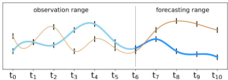
(a) Forecasting regular multivariate time series (MTS)
(a) 预测常规多元时间序列 (MTS)
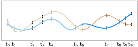
(b) Forecasting irregular multivariate time series (c) Forecasting irregularly sampled multivariate time series with missing values (IMTS)
(b) 预测不规则多元时间序列
(c) 预测带有缺失值的不规则采样多元时间序列 (IMTS)
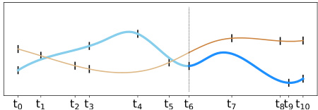
Figure 1: (a) multivariate time series forecasting, (b) irregular multivariate time series forecasting, (c) forecasting irregularly sampled multivariate time series with missing values. In all cases the observation range is from time $t_{0}$ to $t_{6}$ and the forecasting range is from time $t_{7}$ to $t_{10}$ .
图 1: (a) 多元时间序列预测, (b) 不规则多元时间序列预测, (c) 含缺失值的不规则采样多元时间序列预测。所有情况下观测时间范围为 $t_{0}$ 至 $t_{6}$, 预测时间范围为 $t_{7}$ 至 $t_{10}$。
ODE-based models (Schirmer et al. 2022; De Brouwer et al. 2019; Bilos et al.2021; Scholz et al. 2023) are able to forecast at arbitrary time points. However, ODE models can be slow because of their auto-regressive nature and comput ation ally expensive numerical integration process. Also, some ODE models cannot directly handle missing values in the observation space, hence, they often rely on missing value indicators (De Brouwer et al. 2019; Bilos et al. 2021) which are given as additional channels in the data.
基于ODE的模型 (Schirmer et al. 2022; De Brouwer et al. 2019; Bilos et al. 2021; Scholz et al. 2023) 能够在任意时间点进行预测。然而,由于ODE模型的自回归特性和计算成本高昂的数值积分过程,其运行速度可能较慢。此外,部分ODE模型无法直接处理观测空间中的缺失值,因此它们通常依赖作为数据附加通道提供的缺失值指示器 (De Brouwer et al. 2019; Bilos et al. 2021)。
In this work, we propose a novel model called GraFITi: graphs for forecasting IMTS. GraFITi converts IMTS data into a Sparsity Structure Graph and formulates forecasting as edge weight prediction in the graph. This approach represents channels and timepoints as disjoint nodes connected by edges in a bipartite graph. GraFITi uses multiple graph neural network (GNN) layers with attention and feed-forward mechanisms to learn node and edge interactions. Our Sparsity Structure Graph, by design, provides a more dynamic and adaptive approach to process IMTS data, and improves the performance of the forecasting task.
在本工作中,我们提出了一种名为GraFITi的新模型:用于预测不完整多变量时间序列(IMTS)的图结构。GraFITi将IMTS数据转换为稀疏结构图(Sparsity Structure Graph),并将预测问题转化为图中边权重的预测任务。该方法通过二分图将通道和时间点表示为由边连接的不相交节点。GraFITi采用具有注意力机制和前馈机制的多层图神经网络(GNN)来学习节点和边的交互关系。我们设计的稀疏结构图提供了一种更动态、自适应的方法来处理IMTS数据,从而提升了预测任务的性能。
We evaluated GraFITi for forecasting IMTS using 3 realworld and 1 synthetic dataset. Comparing it with state-ofthe-art methods for IMTS and selected baselines for MTS, GraFITi provides superior forecasts.
我们使用3个真实世界数据集和1个合成数据集评估了GraFITi在IMTS预测中的表现。与IMTS领域的最先进方法以及选定的MTS基线模型相比,GraFITi提供了更优的预测结果。
Our contributions are summarized as follows:
我们的贡献总结如下:
• We introduce a novel representation of irregularly sampled multivariate time series with missing values (IMTS) as sparse bipartite graphs, the Sparsity Structure Graph, that efficiently can handle missing values in the observation space of the time series (Section 4). • We propose a novel model based on this representation, GraFITi, that can leverage any graph neural network to perform time series forecasting for IMTS (section 5). • We provide extensive experimental evaluation on 3 real world and 1 synthetic dataset that shows that GraFITi improves the forecasting accuracy of the best existing models by up to $17%$ and the run time improvement up to 5 times (section 6).
• 我们提出了一种新颖的不规则采样多变量时间序列 (IMTS) 表示方法——稀疏二分图 (Sparsity Structure Graph),它能高效处理时间序列观测空间中的缺失值 (第4节)。
• 基于该表示方法,我们提出了一个新模型 GraFITi,可利用任意图神经网络对 IMTS 进行时间序列预测 (第5节)。
• 我们在3个真实数据集和1个合成数据集上进行了大量实验评估,结果表明 GraFITi 将现有最佳模型的预测准确率最高提升 $17%$,运行时间最高加快5倍 (第6节)。
We provide the implementation at https://anonymous.4open.science/r/GraFITi-8F7B.
我们在 https://anonymous.4open.science/r/GraFITi-8F7B 提供了实现。
2 Related Work
2 相关工作
This work focus on the forecasting of irregularly sampled multivariate time series data with missing values using graphs. In this section, we discuss the research done in: forecasting models for IMTS, Graphs for forecasting MTS, and models for edge weight prediction in graphs.
本研究聚焦于利用图结构预测具有缺失值的不规则采样多元时间序列数据(IMTS)。本节将探讨以下领域的研究成果: IMTS预测模型、基于图的MTS预测方法, 以及图中边权重预测模型。
Forecasting of IMTS Research on IMTS has mainly focused on classification (Li and Marlin 2015; Lipton, Kale, and Wetzel 2016; Rubanova, Chen, and Duvenaud 2019; Shukla and Marlin 2021; Horn et al. 2020; Tashiro et al. 2021) and interpolation (Che et al. 2018; Rubanova, Chen, and Duvenaud 2019; Shukla and Marlin 2021; Tashiro et al. 2021; Shukla and Marlin 2022; Yalavarthi, Burchert, and Schmidt-Thieme 2022), with limited attention to forecasting tasks. Existing models for these tasks mostly rely on Neural ODEs (Che et al. 2018). In Latent-ODE (Rubanova, Chen, and Duvenaud 2019), an ODE was combined with a Recurrent Neural Network (RNN) for updating the state at the point of new observation. The GRU-ODE-Bayes model (De Brouwer et al. 2019) improved upon this approach by incorporating GRUs, ODEs, and Bayesian inference for parameter estimation. The Continuous Recurrent Unit (CRU) (Schirmer et al. 2022) based model uses a state-space model with stochastic differential equations and kalman filtering. The recent LinODENet model (Scholz et al. 2023) enhanced CRU by using linear ODEs and ensure self-consistency in the forecasts. Another branch of study involves Neural Flows (Bilos et al. 2021), which use neural networks to model ODE solution curves, rendering the ODE integrator unnecessary. Among various flow architectures, GRU flows have shown good performance.
关于IMTS的研究主要集中在分类 (Li and Marlin 2015; Lipton, Kale, and Wetzel 2016; Rubanova, Chen, and Duvenaud 2019; Shukla and Marlin 2021; Horn et al. 2020; Tashiro et al. 2021) 和插值 (Che et al. 2018; Rubanova, Chen, and Duvenaud 2019; Shukla and Marlin 2021; Tashiro et al. 2021; Shukla and Marlin 2022; Yalavarthi, Burchert, and Schmidt-Thieme 2022) 任务上,对预测任务的关注相对有限。现有模型大多基于神经常微分方程 (Neural ODEs) (Che et al. 2018) 。Latent-ODE (Rubanova, Chen, and Duvenaud 2019) 将ODE与循环神经网络 (RNN) 结合,用于更新新观测点的状态。GRU-ODE-Bayes模型 (De Brouwer et al. 2019) 通过引入门控循环单元 (GRU) 、ODE和贝叶斯推理进行参数估计,改进了这一方法。基于连续循环单元 (CRU) (Schirmer et al. 2022) 的模型采用随机微分方程和卡尔曼滤波的状态空间模型。近期提出的LinODENet模型 (Scholz et al. 2023) 通过线性ODE增强了CRU,并确保预测的自洽性。另一研究方向是神经流 (Neural Flows) (Bilos et al. 2021) ,该技术用神经网络建模ODE解曲线,从而无需ODE积分器。在多种流架构中,GRU流表现出优越性能。
Using graphs for MTS In addition to CNNs, RNNs, and Transformers, graph-based methods have been studied for IMTS forecasting. Early GNN-based approaches, such as (Wu et al. 2020), required a pre-defined adjacency matrix to establish relationships between the time series channels. More recent models like the Spectral Temporal Graph Neural Network (Cao et al. 2020) (STGNN) and the TimeAware Zigzag Network (Chen, Segovia, and Gel 2021) improved on this by using GNNs to capture dependencies between variables in the time series. On the other hand, Satorras, Rangapuram, and Janus chow ski (2022) proposed a bipartite setup with induced nodes to reduce graph complexity, built solely from the channels. Existing graph-based time series forecasting models focus on learning correlations or similarities between channels, without fully exploiting the graph structure. Recently, GNNs were used for imputation and reconstruction of MTS with missing values, treating MTS as sequences of graphs where nodes represent sensors and edges denote correlation (Cini, Marisca, and Alippi 2022; Marisca, Cini, and Alippi 2022). Similar to previous studies, they learn similarity or correlation among channels.
使用图结构处理多元时间序列
除CNN、RNN和Transformer外,基于图的方法也被用于多元时间序列预测。早期基于图神经网络(GNN)的方法(如Wu等人2020年研究)需要预定义邻接矩阵来建立时间序列通道间的关系。近期模型如谱时序图神经网络(Cao等人2020,STGNN)和时序感知锯齿网络(Chen、Segovia与Gel 2021)通过GNN捕捉时间序列变量间的依赖关系进行了改进。另一方面,Satorras、Rangapuram与Januschowski(2022)提出采用诱导节点的二分图结构来降低复杂度,该结构仅由通道构建而成。现有基于图的时间序列预测模型主要关注学习通道间的相关性或相似性,未能充分利用图结构。近期研究(Cini、Marisca与Alippi 2022;Marisca、Cini与Alippi 2022)将GNN用于含缺失值的多元时间序列插补与重建,将多元时间序列视为图序列(节点代表传感器,边表示相关性)。与先前研究类似,这些方法主要学习通道间的相似性或相关性。
Graph Neural Networks for edge weight prediction Graph Neural Networks (GNNs) are designed to process graph-based data. While most GNN literature such as Graph Convolutional Networks, Graph Attention Networks focuses on node classification (Kipf and Welling 2017; Velickovic et al. 2017), a few studies have addressed edge weight prediction. Existing methods (De Sa and Prudencio 2011; Fu et al. 2018) in this domain rely on latent features and graph heuristics, such as node similarity (Zhao et al. 2015), proximity measures (Murata and Moriyasu 2007), and local rankings (Yang and Wang 2020). Recently, deep learning-based approaches (Hou and Holder 2017; Zulaika et al. 2022; You et al. 2020) were proposed. Another branch of research deals with edge weight prediction in weighted signed graphs (Kumar et al. 2016) tailored to social networks. However, all proposed methods typically operate in a trans duct ive setup with a single graph split into training and testing data, which may not be suitable for cases involving multiple graphs like ours, where training and evaluation need to be done on separate graph partitions.
用于边权重预测的图神经网络
图神经网络 (Graph Neural Networks, GNNs) 专为处理基于图结构的数据而设计。虽然大多数GNN文献(如图卷积网络、图注意力网络)主要关注节点分类 (Kipf and Welling 2017; Velickovic et al. 2017),但已有少量研究涉及边权重预测。该领域的现有方法 (De Sa and Prudencio 2011; Fu et al. 2018) 依赖于潜在特征和图启发式方法,例如节点相似性 (Zhao et al. 2015)、邻近度测量 (Murata and Moriyasu 2007) 和局部排序 (Yang and Wang 2020)。近年来,基于深度学习的方法 (Hou and Holder 2017; Zulaika et al. 2022; You et al. 2020) 被提出。另一研究方向针对社交网络场景,研究带符号加权图中的边权重预测问题 (Kumar et al. 2016)。然而,现有方法通常采用直推式 (transductive) 设定,即将单个图划分为训练集和测试集,这不适用于涉及多个图的情况(如本文场景),此类场景需要在独立的图分区上进行训练和评估。
3 The Time Series Forecasting Problem
3 时间序列预测问题
An irregularly sampled multivariate times series with missing values, is a finite sequence of pairs $\boldsymbol{S}\quad=\quad$ $(t_{n},x_{n}){n=1:N}$ where $t_{n}\in\mathbb{R}$ is the $n$ -th observation time- point and $x_{n}\in(\mathbb{R}\cup{\mathtt{N a N}})^{C}$ is the $n$ -th observation event. Components with $x_{n,c}\neq\mathtt{N a N}$ represent observed values by channel $c$ at event time $t_{n}$ , and $x_{n,c}=\tt N a N$ represents a missing value. $C$ is the total number of channels.
一个具有缺失值的不规则采样多元时间序列,可以表示为一个有限的序列对 $\boldsymbol{S}\quad=\quad$ $(t_{n},x_{n}){n=1:N}$ ,其中 $t_{n}\in\mathbb{R}$ 是第 $n$ 个观测时间点, $x_{n}\in(\mathbb{R}\cup{\mathtt{N a N}})^{C}$ 是第 $n$ 个观测事件。当 $x_{n,c}\neq\mathtt{N a N}$ 时,表示通道 $c$ 在时间 $t_{n}$ 处观测到的值;若 $x_{n,c}=\tt N a N$ 则表示缺失值。 $C$ 为通道总数。
A time series query is a pair $(Q,S)$ of a time series $S$ and a sequence $Q=(q_{k},c_{k}){k=1:K}$ such that the value of channel $c_{k}\in{1,\ldots,C}$ is to be predicted at time $q_{k}\in\mathbb{R}$ . We call a query a forecasting query, if all its query timepoints are after the last timepoint of the time series $S$ , an imputation query if all of them are before the last timepoint of $S$ and a mixed query otherwise. In this paper, we are interested in forecasting only.
时间序列查询是一对 $(Q,S)$,其中 $S$ 是一个时间序列,$Q=(q_{k},c_{k}){k=1:K}$ 是一个序列,要求在时间 $q_{k}\in\mathbb{R}$ 预测通道 $c_{k}\in{1,\ldots,C}$ 的值。如果查询的所有时间点都在时间序列 $S$ 的最后一个时间点之后,则称之为预测查询;如果所有时间点都在 $S$ 的最后一个时间点之前,则称为填补查询;否则称为混合查询。本文仅关注预测查询。
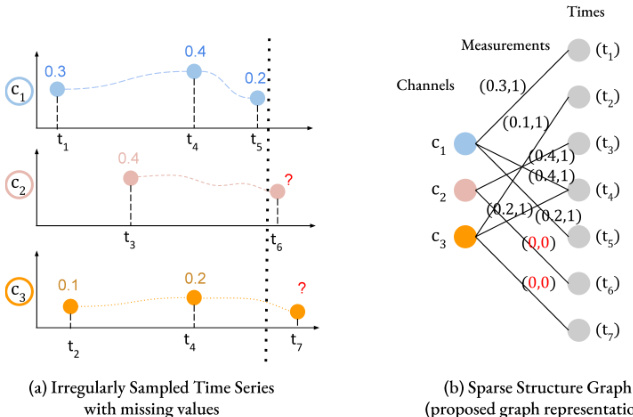
Figure 2: Representation of IMTS as Sparsity Structure Graph. (b) is the Sparsity Structure Graph representation of (a) where times and channels are the nodes and observation measurements are the edges with observations values. Target edges are provided with $(0,0)$ .
图 2: IMTS作为稀疏结构图的表示。(b)是(a)的稀疏结构图表示,其中时间和通道是节点,观测测量值是带有观测值的边。目标边被赋予$(0,0)$。
A vector $y\in\mathbb{R}^{K}$ we call an answer to the forecasting query: $y_{k}$ is understood as the predicated value of time series $S$ at time $q_{k}$ in channel $c_{k}$ . The difference between two answers $y,y^{\prime}$ to the same query can be measured by any loss function, for example by a simple squared error
向量 $y\in\mathbb{R}^{K}$ 被称为预测查询的答案:$y_{k}$ 表示时间序列 $S$ 在通道 $c_{k}$ 中时间点 $q_{k}$ 处的预测值。对于同一查询的两个答案 $y,y^{\prime}$ 之间的差异,可以通过任何损失函数来衡量,例如简单的平方误差。
$$
\ell(y,y^{\prime}):=\frac{1}{K}\sum_{k=1}^{K}(y_{k}-y_{k}^{\prime})^{2}
$$
$$
\ell(y,y^{\prime}):=\frac{1}{K}\sum_{k=1}^{K}(y_{k}-y_{k}^{\prime})^{2}
$$
The time series forecasting problem is as follows: given a dataset of pairs $D:=(\bar{Q_{i}},\bar{S_{i}},y_{i})_{i=1:M}$ of forecasting queries and ground truth answers from an unknown distribution $p^{\mathrm{data}}$ and a loss function $\ell$ on forecasting answers, find a forecasting model $\hat{y}$ that maps queries $(Q,S)$ to answers $\hat{y}(Q,S)$ such that the expected loss between ground truth answers and forecasted answers is minimal:
时间序列预测问题定义如下:给定来自未知分布 $p^{\mathrm{data}}$ 的预测查询与真实答案配对数据集 $D:=(\bar{Q_{i}},\bar{S_{i}},y_{i})_{i=1:M}$ ,以及预测答案的损失函数 $\ell$ ,需找到一个预测模型 $\hat{y}$ ,该模型将查询 $(Q,S)$ 映射为预测答案 $\hat{y}(Q,S)$ ,使得真实答案与预测答案之间的期望损失最小:
$$
\mathcal{L}(\boldsymbol{\hat{y}};\boldsymbol{p}^{\mathrm{data}}):=\mathbb{E}_{(Q,S,y)\sim p^{\mathrm{data}}}\big[\ell(\boldsymbol{y},\boldsymbol{\hat{y}}(Q,S))\big]
$$
$$
\mathcal{L}(\boldsymbol{\hat{y}};\boldsymbol{p}^{\mathrm{data}}):=\mathbb{E}_{(Q,S,y)\sim p^{\mathrm{data}}}\big[\ell(\boldsymbol{y},\boldsymbol{\hat{y}}(Q,S))\big]
$$
4 Sparsity Structure Graph Representation
4 稀疏结构图表示
We describe the proposed Sparsity Structure Graph represent ation and convert the forecasting problem as edge weight prediction problem. Using the proposed representation:
我们描述了所提出的稀疏结构图表示方法,并将预测问题转化为边权重预测问题。利用该表示方法:
• We explicitly obtain the relationship between the channels and times via observation values allowing the inductive bias of the data to pass into the model. • We elegantly handle the missing values in IMTS in the observation space by connecting edges only for the observed values.
• 我们通过观测值明确获取通道与时间的关系,使数据的归纳偏差能够传递到模型中。
• 我们通过在观测空间中仅对观测值建立连接边,优雅地处理了IMTS中的缺失值问题。
Missing values represented by NaN-values are unsuited for standard arithmetical operations. Therefore, they are often encoded by dedicated binary variables called missing value indicators or masks: $\overline{{x_{n}}}\in(\mathbb{R}\times{0,1})^{C}$ . Here, $(x_{n,c,1},1)$ encodes an observed value and $(0,0)$ encodes a missing value. Usually, both components are seen as different scalar variables: the real value $x_{n,c,1}$ and its binary missing value indicator / mask $x_{n,c,2}$ , the relation between both is dropped and observations simply modeled as $x_{n}\in\mathbb{R}^{2C}$ .
用NaN值表示的缺失值不适合进行标准算术运算。因此,它们通常通过专门的二元变量(称为缺失值指示器或掩码)进行编码:$\overline{{x_{n}}}\in(\mathbb{R}\times{0,1})^{C}$。其中,$(x_{n,c,1},1)$表示观测值,$(0,0)$表示缺失值。通常,这两个分量被视为不同的标量变量:实数值$x_{n,c,1}$及其二元缺失值指示器/掩码$x_{n,c,2}$,两者之间的关系被忽略,观测值简化为$x_{n}\in\mathbb{R}^{2C}$。
We propose a novel representation of a time series $S$ using a bipartite graph $G\doteq(V,E)$ . The graph has nodes for channels and timepoints, denoted as $V_{C}$ and $V_{T}$ respectively $(V=V_{C}\cup V_{T})$ . Edges $E\subseteq V_{C}\times V_{T}$ in the graph connect each channel node to its corresponding timepoint node with an observation. Edge features $F^{\mathrm{edge}}$ are the observation values and node features $F^{\mathrm{node}}$ are the channel IDs and timepoints. Nodes $V_{C}:={1,\dots,C}$ represent channels and nodes 。
我们提出了一种新颖的时间序列$S$表示方法,采用二分图$G\doteq(V,E)$。该图包含通道节点和时间点节点,分别记为$V_{C}$和$V_{T}$ $(V=V_{C}\cup V_{T})$。图中的边$E\subseteq V_{C}\times V_{T}$将每个通道节点与其对应观测值的时间点节点相连。边特征$F^{\mathrm{edge}}$为观测值,节点特征$F^{\mathrm{node}}$为通道ID和时间点。通道节点$V_{C}:={1,\dots,C}$表示通道。
For an IMTS, missing values make the bipartite graph sparse, meaning $|E|\ll C\cdot N$ . However, for a fully observed time series, where there are no missing values, i.e. $|E|=C\cdot N$ , the graph is a complete bipartite graph.
对于一个IMTS (Incomplete Multivariate Time Series) ,缺失值会导致二分图变得稀疏,这意味着 $|E|\ll C\cdot N$ 。然而,对于一个完全观测到的时间序列,即没有缺失值的情况 $|E|=C\cdot N$ ,该图就是一个完全二分图。
We extend this representation to time series queries $(S,Q)$ by adding additional edges between queried channels and timepoints, and distinguish observed and queried edges by an additional binary edge feature called target indicator. Note that the target indicator used to differentiate the observed edge and target edge is different from the missing value indicator which is used to represent the missing observations in the observation space. Given a query ${\cal Q}={}$ $(q_{k},c_{k}){k=1:K}$ , let $(t_{1}^{\prime},\dots,t_{K^{\prime}}^{\prime})$ be an enumeration of the unique queried timepoints $q_{k}$ . We introduce additional nodes $V_{Q}:={C+N+1,\dots,C+N+K^{\prime}}$ 。
我们将这种表示扩展到时间序列查询 $(S,Q)$,方法是在查询的通道和时间点之间添加额外的边,并通过一个称为目标指示器的二元边特征来区分已观测边和查询边。需要注意的是,用于区分已观测边和目标边的目标指示器,与用于表示观测空间中缺失观测值的缺失值指示器不同。给定查询 ${\cal Q}={}$ $(q_{k},c_{k}){k=1:K}$,令 $(t_{1}^{\prime},\dots,t_{K^{\prime}}^{\prime})$ 为唯一查询时间点 $q_{k}$ 的枚举。我们引入额外的节点 $V_{Q}:={C+N+1,\dots,C+N+K^{\prime}}$。
where $\begin{array}{r l r}{\left(t_{i-N-C}^{\prime},j\right)}&{{}\in}&{Q}\end{array}$ is supposed to mean that $(t_{i-N-C}^{\prime},j)$ appears in the sequence $Q$ . To denote this graph representation, we write briefly
其中 $\begin{array}{r l r}{\left(t_{i-N-C}^{\prime},j\right)}&{{}\in}&{Q}\end{array}$ 表示 $(t_{i-N-C}^{\prime},j)$ 出现在序列 $Q$ 中。为简洁表示该图结构,我们简记为
$$
\mathrm{ts}2\mathrm{graph}(X,Q):=(V,E,F^{\mathrm{node}},F^{\mathrm{edge}})
$$
$$
\mathrm{ts}2\mathrm{graph}(X,Q):=(V,E,F^{\mathrm{node}},F^{\mathrm{edge}})
$$
The conversion of an IMTS to a Sparsity Structure Graph is shown in Figure 2.
图 2: IMTS转换为稀疏结构图的示意图
To make the graph representation $(V,E,F^{\mathrm{node}},F^{\mathrm{edge}})$ of a time series query process able by a graph neural network, node and edge features have to be properly embedded, otherwise, both, the nominal channel ID and the timepoint are hard to compute on. We propose an Initial Embedding layer that encodes channel IDs via a onehot encoding and time points via a learned sinusoidal encoding (Shukla and Marlin 2021)
为了使时序查询过程的图表示 $(V,E,F^{\mathrm{node}},F^{\mathrm{node}})$ 能够被图神经网络处理,节点和边的特征必须被适当嵌入,否则名义通道ID和时间点都难以计算。我们提出了一个初始嵌入层,该层通过独热编码 (onehot encoding) 对通道ID进行编码,并通过学习到的正弦编码 (Shukla and Marlin 2021)
where onehot denotes the binary indicator vector and FF denotes a separate fully connected layer in each case.
其中onehot表示二进制指示向量,FF在每种情况下表示一个独立的全连接层。
The final graph neural network layer $(h^{\mathrm{node},L},h^{\mathrm{edge},L})$ has embedding dimension 1. The scalar values of the query edges are taken as the predicted answers to the encoded forecasting query:
最终的图神经网络层 $(h^{\mathrm{node},L},h^{\mathrm{edge},L})$ 的嵌入维度为1。查询边的标量值被视为对编码预测查询的预测答案:
$$
\begin{array}{r}{\hat{y}:=\mathrm{graph}2\mathrm{ts}(h^{\mathrm{node},L},h^{\mathrm{edge},L},V,E)=(h_{e_{k}}^{\mathrm{edge},L}){k=1:K}}\ {\mathrm{where}~e_{k}={C+N+k^{\prime},c_{k}}\quad\mathrm{with}\quad t_{k^{\prime}}^{\prime}=q_{k}}\end{array}
$$
$$
\begin{array}{r}{\hat{y}:=\mathrm{graph}2\mathrm{ts}(h^{\mathrm{node},L},h^{\mathrm{edge},L},V,E)=(h_{e_{k}}^{\mathrm{edge},L}){k=1:K}}\ {\mathrm{where}~e_{k}={C+N+k^{\prime},c_{k}}\quad\mathrm{with}\quad t_{k^{\prime}}^{\prime}=q_{k}}\end{array}
$$
5 Forecasting with GraFITi
5 使用 GraFITi 进行预测
GraFITi first encodes the time series query to graph using Eq. 4 and compute initial embeddings for the nodes $(h^{\mathrm{node,0^{-}}})$ and edges $(h^{\mathrm{edge},0})$ using Eqs. 5 and 6 respectively. Now, we can leverage the power of graph neural networks for further processing the encoded graph. Node and edge features are updated layer wise, from layer $l$ to $l+1$ using a graph neural network:
GraFITi首先通过公式4将时间序列查询编码为图,并分别使用公式5和公式6计算节点$(h^{\mathrm{node,0^{-}}})$和边$(h^{\mathrm{edge},0})$的初始嵌入。现在,我们可以利用图神经网络(graph neural network)的力量进一步处理编码后的图。节点和边的特征通过图神经网络逐层更新,从层$l$到$l+1$:
$$
(h^{\mathrm{node},l+1},h^{\mathrm{edge},l+1}):=\mathrm{gnn}^{(l)}(h^{\mathrm{node},l},h^{\mathrm{edge},l},V,E)
$$
$$
(h^{\mathrm{node},l+1},h^{\mathrm{edge},l+1}):=\mathrm{gnn}^{(l)}(h^{\mathrm{node},l},h^{\mathrm{edge},l},V,E)
$$
There have been a variety of gnn architectures such as Graph Convolutional Networks (Kipf and Welling 2017), Graph Attention Networks (Velickovic et al. 2017), proposed in the literature. In this work, we propose a model adapting the Graph Attention Network (Velickovic et al. 2017) to our graph setting and incorporate essential components for handling sparsity structure graphs. While a Graph Attention Network computes attention weights by adding queries and keys, we found no advantage in using this approach (see supplementary material). Thus, we utilize standard attention mechanism, in our attention block, as it has been widely used in the literature (Zhou et al. 2021). Additionally, we also use edge embeddings in our setup to update node embeddings in a principled manner.
已有多种图神经网络架构被提出,如图卷积网络 (Kipf and Welling 2017) 、图注意力网络 (Velickovic et al. 2017) 。本工作基于图注意力网络 (Velickovic et al. 2017) 进行适应性改造,针对稀疏结构图的特点融入了关键组件。虽然原始图注意力网络通过叠加查询向量和键向量来计算注意力权重,但实验表明该方法并无优势 (详见补充材料) 。因此,我们采用文献 (Zhou et al. 2021) 中广泛使用的标准注意力机制作为注意力模块的核心。此外,我们还通过边嵌入 (edge embeddings) 以规范化方式更新节点嵌入。
Graph Neural Network (gnn)
图神经网络 (GNN)
First, we define Multi-head Attention block (MAB) and Neighborhood functions that are used in our gnn.
首先,我们定义用于图神经网络 (gnn) 的多头注意力块 (MAB) 和邻域函数。
A Multi-head attention block (MAB) (Vaswani et al. 2017) is represented as:
多头注意力块 (MAB) (Vaswani et al. 2017) 表示为:
$$
\begin{array}{r}{\mathbf{MAB}(\mathcal{Q},\mathcal{K},\mathcal{V}):=\alpha(\mathcal{H}+\mathbf{FF}(\mathcal{H}))\quad\quad}\ {\quad\mathrm{where}\quad\mathcal{H}:=\alpha(\mathcal{Q}+\mathbf{MHA}(\mathcal{Q},\mathcal{K},\mathcal{V}))}\end{array}
$$
$$
\begin{array}{r}{\mathbf{MAB}(\mathcal{Q},\mathcal{K},\mathcal{V}):=\alpha(\mathcal{H}+\mathbf{FF}(\mathcal{H}))\quad\quad}\ {\quad\mathrm{where}\quad\mathcal{H}:=\alpha(\mathcal{Q}+\mathbf{MHA}(\mathcal{Q},\mathcal{K},\mathcal{V}))}\end{array}
$$
where $\mathcal{Q},\mathcal{K}$ and, $\nu$ are called queries, keys, and values respectively, MHA is multi-head attention (Vaswani et al. 2017), $\alpha$ is a non-linear activation.
其中 $\mathcal{Q}$、$\mathcal{K}$ 和 $\nu$ 分别称为查询 (queries)、键 (keys) 和值 (values),MHA 是多头注意力机制 (multi-head attention) (Vaswani et al. 2017),$\alpha$ 是非线性激活函数。
Algorithm 1: Graph Neural Network $(\mathbf{g}\mathbf{n}\mathbf{n}^{(l)})$ )
算法 1: 图神经网络 (Graph Neural Network, $\mathbf{g}\mathbf{n}\mathbf{n}^{(l)}$)
| 输入: hnode,l | ,hedge,l, V, E |
|---|---|
| for u ∈ V do | Hu← ([hnode,l |
| lle={u,u} | |
| for e = {u,v} ∈ E do | |
| — | + FF(l) hnode,l hedge,l e |
| 输出 | hedge,l+1 |
The Neighborhood of a node $u$ is defined as the set of all the nodes connected to $u$ through edges in $E$ :
节点 $u$ 的邻域 (Neighborhood) 定义为通过边集 $E$ 与 $u$ 相连的所有节点集合:
$$
\mathcal{N}(u):={v\mid{u,v}\in E}
$$
$$
\mathcal{N}(u):={v\mid{u,v}\in E}
$$
GraFITi consists of $L$ gnnlayers. In each layer, node embeddings are updated using neighbor node embeddings and edge embeddings connecting them. For edge embeddings, we use the embeddings of the adjacent nodes and the current edge embedding. The overall architecture of GraFITi is shown in Figure 3.
GraFITi由$L$个GNN层组成。每一层中,节点嵌入通过相邻节点嵌入及连接它们的边嵌入进行更新。对于边嵌入,我们使用相邻节点的嵌入和当前边嵌入。GraFITi的整体架构如图3所示。
Update node embeddings To update embedding of a node $u\in V$ , first, we create a sequence of features $H_{u}$ concatenating its neighbor node embedding $h_{v}^{\mathrm{node},l}$ and edge embedding heedge,l, $h_{e}^{\mathrm{edge},l},e={u,v}$ where $v\in\mathcal{N}(u)$ . We then pass hnode,l as queries and $H_{u}$ as keys and values to MAB.
更新节点嵌入
为了更新节点 $u\in V$ 的嵌入,首先我们创建一个特征序列 $H_{u}$,将其邻居节点嵌入 $h_{v}^{\mathrm{node},l}$ 和边嵌入 $h_{e}^{\mathrm{edge},l},e={u,v}$ 拼接起来,其中 $v\in\mathcal{N}(u)$。接着,我们将 $h_{v}^{\mathrm{node},l}$ 作为查询,$H_{u}$ 作为键和值输入到 MAB 中。
$$
\begin{array}{r l}&{h_{u}^{\mathrm{node},l+1}:=\mathbf{M}\mathbf{A}\mathbf{B}^{(l)}\left(h_{u}^{\mathrm{node},l},H_{u},H_{u}\right)}\ &{\qquadH_{u}:=\left(\left[h_{v}^{\mathrm{node},l}\parallel h_{e}^{\mathrm{edge},l}\right]\right)_{v\in\mathcal{N}(u)},e={u,v}}\end{array}
$$
$$
\begin{array}{r l}&{h_{u}^{\mathrm{node},l+1}:=\mathbf{M}\mathbf{A}\mathbf{B}^{(l)}\left(h_{u}^{\mathrm{node},l},H_{u},H_{u}\right)}\ &{\qquadH_{u}:=\left(\left[h_{v}^{\mathrm{node},l}\parallel h_{e}^{\mathrm{edge},l}\right]\right)_{v\in\mathcal{N}(u)},e={u,v}}\end{array}
$$
Updating edge embeddings: To compute edge embedding $h_{e}^{\mathrm{edge},l+1}$ , $e={u,v}$ we concatenate $h_{u}^{\mathrm{node},l},h_{v}^{\mathrm{node},l}$ and $h_{e}^{\mathrm{edge},l}$ , and pass it through a dense layer (FF) followed by a residual connection and nonlinear activation.
更新边嵌入(edge embeddings):为了计算边嵌入 $h_{e}^{\mathrm{edge},l+1}$ (其中 $e={u,v}$),我们将 $h_{u}^{\mathrm{node},l},h_{v}^{\mathrm{node},l}$ 和 $h_{e}^{\mathrm{edge},l}$ 拼接起来,然后通过一个稠密层(FF),接着进行残差连接和非线性激活。
$$
h_{e}^{\mathrm{{edge}},l+1}:=\alpha\left(h_{e}^{\mathrm{{edge}},l}+\mathbf{F}\mathbf{F}^{(l)}\left(h_{u}^{\mathrm{{node}},l}\parallel h_{v}^{\mathrm{{node}},l}\parallel h_{e}^{\mathrm{{edge}},l}\right)\right)
$$
$$
h_{e}^{\mathrm{{edge}},l+1}:=\alpha\left(h_{e}^{\mathrm{{edge}},l}+\mathbf{F}\mathbf{F}^{(l)}\left(h_{u}^{\mathrm{{node}},l}\parallel h_{v}^{\mathrm{{node}},l}\parallel h_{e}^{\mathrm{{edge}},l}\right)\right)
$$
where $e={u,v}$ . Note that, although our edges are undirected, we compute the edge embedding by concatenating the embeddings in a specific order i.e., the channel embedding, time embedding and edge embedding. We show the process of updating nodes and edges in layer $l$ using a gnnin Algorithm 1.
其中 $e={u,v}$。需要注意的是,虽然我们的边是无向的,但我们通过按特定顺序拼接嵌入来计算边嵌入,即通道嵌入、时间嵌入和边嵌入。我们在算法1中使用gnn展示了第 $l$ 层中节点和边的更新过程。
Answering the queries: As mentioned in Section 4, our last $\mathrm{gnn}^{(L)}$ layer has embedding dimension 1. Hence, after processing the graph features through $L$ many gnn layers, we use Eq. 7 to decode the graph and provide the predicted answers to the time series query. A forward pass of GraFITi is presented in Algorithm 2.
回答问题:如第4节所述,我们的最后一层$\mathrm{gnn}^{(L)}$嵌入维度为1。因此,在通过$L$个gnn层处理图特征后,我们使用公式7对图进行解码,并为时间序列查询提供预测答案。GraFITi的前向传播过程如算法2所示。
Computational Complexity: The computational complexity of GraFITi primarily comes from using MAB in Eq. 11. For a single channel node $u\in{1,...,C}$ , the maximum complexity for computing its embedding is $\mathcal{N}(u)$ since only neighborhood connections are used for the update, and $\mathcal{N}(\boldsymbol{\bar{u}})\subseteq{\boldsymbol{C}+1,...,\boldsymbol{C}+\boldsymbol{N}+\boldsymbol{K}^{\prime}}$ . Thus, computing the embeddings of all channel nodes is $\mathcal O(|E|)$ . Similarly, the computational complexity of MAB for computing the embeddings of all nodes in $V_{T}\cup V_{Q}$ is also $\mathcal{\bar{O}}(|E|)$ . A feed forward layer $\mathbf{F}\mathbf{F}:\mathbb{R}^{Y}\rightarrow\mathbb{R}^{Z}$ will have a computational complexity of $\mathcal{O}(Y Z)$ .
计算复杂度:GraFITi的计算复杂度主要来自公式11中使用的多臂老虎机 (MAB) 。对于单个通道节点 $u\in{1,...,C}$ ,计算其嵌入的最大复杂度为 $\mathcal{N}(u)$ ,因为更新时仅使用邻域连接,且 $\mathcal{N}(\boldsymbol{\bar{u}})\subseteq{\boldsymbol{C}+1,...,\boldsymbol{C}+\boldsymbol{N}+\boldsymbol{K}^{\prime}}$ 。因此,计算所有通道节点的嵌入复杂度为 $\mathcal O(|E|)$ 。同理,MAB计算 $V_{T}\cup V_{Q}$ 中所有节点嵌入的计算复杂度也是 $\mathcal{\bar{O}}(|E|)$ 。前馈层 $\mathbf{F}\mathbf{F}:\mathbb{R}^{Y}\rightarrow\mathbb{R}^{Z}$ 的计算复杂度为 $\mathcal{O}(Y Z)$ 。
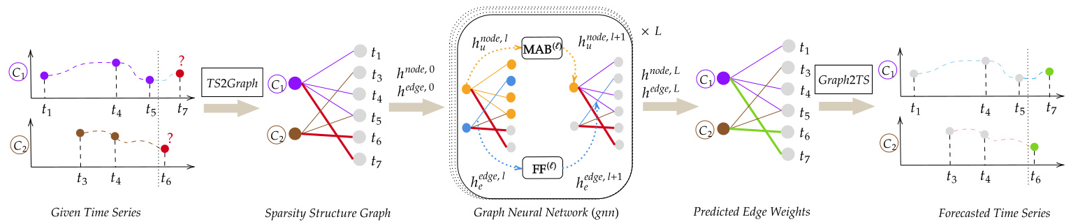
Figure 3: Overall architecture of GraFITi.
图 3: GraFITi的整体架构。
算法 2: GraFITi前向传播
确保: 观测时间序列预测查询 (S, Q)
(V,E, Fnode, Fedge) ← ts2graph(S, Q) //式4
//式5
//节点和边的初始嵌入
hnode,0 {An hedge,0 ↑人
{u,u} ∈E} //式6
//图神经网络
for l ∈ {1, ..., L} do ,V,E) //算法1
y ← graph2ts(hnode,L , hedge,L, ,V,E) //式7
Delineating from GRAPE (You et al. 2020) You et al. (2020) introduced GRAPE, a graph-based model for imputing and classifying vector datasets with missing values. This approach employs a bipartite graph, with nodes divided into separate sets for sample IDs and sample features. The edges of this graph represent the feature values associated with the samples. Notably, GRAPE learns in a trans duct ive manner, encompassing all the data samples, including those from the test set, within in the graph. In contrast, GraFITi uses inductive approach. Here, each instance is a Sparsity Structure Graph, tailored for time series data. In this structure, nodes are divided into distinct sets for channels and timepoints, while the edges are the time series observations.
区别于GRAPE (You et al. 2020)
You et al. (2020) 提出了GRAPE, 这是一种基于图的模型, 用于对含缺失值的向量数据集进行填补和分类。该方法采用二分图结构, 节点分为样本ID和样本特征两个独立集合, 图的边则代表样本对应的特征值。值得注意的是, GRAPE以直推式 (transductive) 方式学习, 图中包含所有数据样本 (包括测试集样本) 。而GraFITi采用归纳式 (inductive) 方法, 其中每个实例都是一个专为时间序列数据设计的稀疏结构图 (Sparsity Structure Graph) 。该结构中, 节点分为通道和时间点两个独立集合, 边则代表时间序列观测值。
6 Experiments
6 实验
Table 1: Statistics of the datasets used in the experiments. Sparsity means the percentage of missing observations in the time series
表 1: 实验所用数据集的统计信息。稀疏度表示时间序列中缺失观测值的百分比
| Name | #Sample | #Chann. | Max.len. | Max.Obs. | Sparsity |
|---|---|---|---|---|---|
| USHCN | 1,100 | 5 | 290 | 320 | 77.9% |
| MIMIC-III | 21,000 | 96 | 96 | 710 | 94.2% |
| MIMIC-IV | 18,000 | 102 | 710 | 1340 | 97.8% |
| Physionet'12 | 12,000 | 37 | 48 | 520 | 85.7% |
6.1 Dataset description
6.1 数据集描述
4 datasets including 3 real world medical and 1 synthetic climate IMTS datasets are used for evaluating the proposed model. Basic statistics of the datasets is provided in Table 1.
用于评估所提出模型的数据集包括3个真实世界医疗和1个合成气候IMTS数据集。数据集的基本统计信息如表1所示。
Physionet’12 (Silva et al. 2012) consists of ICU patient records observed for 48 hours. MIMIC-III (Johnson et al. 2016) is also a medical dataset that consists measurements of the ICU patients observed for 48 hours. MIMICIV (Johnson et al. 2021) is built upon the MIMIC-III database. USHCN (Menne, Williams Jr, and Vose 2015) is a climate dataset that consists of the measurements of daily temperatures, precipitation and snow observed over 150 years from 1218 meteorological stations in the USA. For MIMIC-III, MIMIC-IV and USHCN, we followed the pre-processing steps provided by Scholz et al. (2023); Bilos et al. (2021); De Brouwer et al. (2019). Hence, observations in MIMIC-III and MIMIC-IV are rounded for 30 mins and 1 hour respectively. Whereas for the Physionet’12, we follow the protocol of Che et al. (2018); Cao et al. (2018); Tashiro et al. (2021) and processed the dataset to have hourly observations.
Physionet'12 (Silva et al. 2012) 包含ICU患者48小时内的观测记录。MIMIC-III (Johnson et al. 2016) 同样是一个医疗数据集,记录了ICU患者48小时内的测量数据。MIMICIV (Johnson et al. 2021) 基于MIMIC-III数据库构建。USHCN (Menne, Williams Jr, and Vose 2015) 是一个气候数据集,包含美国1218个气象站150年来每日温度、降水和降雪的观测数据。对于MIMIC-III、MIMIC-IV和USHCN,我们遵循了Scholz等 (2023)、Bilos等 (2021) 和De Brouwer等 (2019) 提供的预处理步骤。因此,MIMIC-III和MIMIC-IV中的观测数据分别按30分钟和1小时进行取整。而对于Physionet'12,我们遵循Che等 (2018)、Cao等 (2018) 和Tashiro等 (2021) 的方案,将数据集处理为每小时观测一次。
6.2 Competing algorithms
6.2 竞争算法
Here, we provide brief details of the models that are compared with the proposed GraFITi for evaluation.
在此,我们简要介绍与所提出的GraFITi进行比较评估的模型详情。
We select 4 IMTS forecasting models for comparison, including GRU-ODE-Bayes (De Brouwer et al. 2019), Neural Flows (Bilos et al. 2021), CRU (Schirmer et al. 2022) and LinODENet (Scholz et al. 2023). Additionally, we use the well established IMTS interpolation model mTAN (Shukla and Marlin 2021). It is interesting to verify the performance of well established MTS forecasting models for IMTS setup. We do this by adding missing value indicators as the separate channels to the series and process the time series along with the missing value indicators. Hence we compare with Informer+, Fedformer+, DLinear+ and NLinear+ which are variants of Informer (Zhou et al. 2021), FedFormer (Zhou et al. 2022), DLinear and NLinear (Zeng et al. 2022) respectively. We also compare with the published results from (De Brouwer et al. 2019) for the NeuralODE-VAE (Chen et al. 2018), Sequential VAE (Krishnan, Shalit, and Sontag 2015, 2017), GRUSimple (Che et al. 2018), GRU-D (Che et al. 2018) and TLSTM (Baytas et al. 2017).
我们选取了4种IMTS预测模型进行比较,包括GRU-ODE-Bayes (De Brouwer et al. 2019)、Neural Flows (Bilos et al. 2021)、CRU (Schirmer et al. 2022)和LinODENet (Scholz et al. 2023)。此外,我们使用了成熟的IMTS插值模型mTAN (Shukla and Marlin 2021)。验证成熟的多时间序列预测模型在IMTS设置下的性能具有研究价值,为此我们通过将缺失值指示器作为独立通道添加到序列中,并与缺失值指示器一起处理时间序列。因此我们比较了Informer+、Fedformer+、DLinear+和NLinear+,它们分别是Informer (Zhou et al. 2021)、FedFormer (Zhou et al. 2022)、DLinear和NLinear (Zeng et al. 2022)的变体。我们还与(De Brouwer et al. 2019)发表的NeuralODE-VAE (Chen et al. 2018)、Sequential VAE (Krishnan, Shalit, and Sontag 2015, 2017)、GRUSimple (Che et al. 2018)、GRU-D (Che et al. 2018)和TLSTM (Baytas et al. 2017)的结果进行了对比。
Table 2: Experimental results for forecasting next three time steps. Evaluation metric MSE, Lower is better. Best results are in bold and the next best are in italics. Published results are presented in open brackets, Physionet’12 dataset was not used by the baseline models hence do not have published results. We show % improvement with $\uparrow$ . ‘ME’ indicates Memory Error.
表 2: 未来三个时间步预测的实验结果。评估指标为MSE (均方误差),数值越低越好。最佳结果加粗显示,次佳结果以斜体标注。已发表结果用圆括号标注,基线模型未使用Physionet'12数据集故无发表结果。改进百分比用 $\uparrow$ 表示,'ME'表示内存错误。
| USHCN | MIMIC-III | MIMIC-IV | Physionet'12 | |
|---|---|---|---|---|
| DLinear+ | 0.347 ± 0.065 | 0.691 ± 0.016 | 0.577 ± 0.001 | 0.380 ± 0.001 |
| NLinear+ | 0.452 ± 0.101 | 0.726 ± 0.019 | 0.620 ± 0.002 | 0.382 ± 0.001 |
| Informer+ | 0.320 ± 0.047 | 0.512 ± 0.064 | 0.420 ± 0.007 | 0.347 ± 0.001 |
| FedFormer+ | 2.990 ± 0.476 | 1.100 ± 0.059 | 2.135±0.304 | 0.455±0.004 |
| NeuralODE-VAE | (0.960 ± 0.110) | (0.890 ± 0.010) | ||
| SequentialVAE | (0.830 ± 0.070) | (0.920 ± 0.090) | ||
| GRU-Simple | (0.750 ± 0.120) | (0.820 ± 0.050) | ||
| GRU-D | (0.530 ± 0.060) | (0.790 ± 0.060) | ||
| T-LSTM | (0.590 ± 0.110) | (0.620 ± 0.050) | ||
| mTAN | 0.300 ±0.038 | 0.540 ± 0.036 | ME | 0.315 ± 0.002 |
| GRU-ODE-Bayes | 0.401 ± 0.089 (0.430 ± 0.070) | 0.476 ± 0.043 (0.480 ± 0.010) | 0.360 ± 0.001 (0.379 ± 0.005) | 0.329 ± 0.004 |
| Neural Flow | 0.414 ± 0.102 | 0.477 ± 0.041 (0.490 ± 0.004) | 0.354 ± 0.001 (0.364 ± 0.008) | 0.326 ± 0.004 |
| CRU | 0.290 ± 0.060 | 0.592 ± 0.049 | ME | 0.379 ± 0.003 |
| LinODEnet | 0.300 ± 0.060 (0.290 ± 0.060) | 0.446 ± 0.033 (0.450 ± 0.020) | 0.272 ± 0.002 (0.274 ± 0.002) | 0.299 ± 0.001 |
| GraFITi (ours) | 0.272±0.047↑ 9.3% | 0.396±0.030↑11.2% | 0.225± 0.001↑ 17.2% | 0.286±0.001↑4.3% |
6.3 Experimental setup
6.3 实验设置
Task protocol We followed Scholz et al. (2023); Bilos et al. (2021); De Brouwer et al. (2019), applied 5-fold cross-validation and selected hyper parameters using a holdout validation set $(20%)$ . For evaluation, we used $10%$ unseen data. All models were trained on Mean Squared Error, which is also the evaluation metric.
任务协议
我们遵循 Scholz et al. (2023) 、 Bilos et al. (2021) 和 De Brouwer et al. (2019) 的方法,采用 5 折交叉验证,并使用保留验证集 $(20%)$ 选择超参数。评估时,我们使用了 $10%$ 的未见数据。所有模型均以均方误差 (Mean Squared Error) 为训练目标,该指标也作为评估标准。
Hyper param ter search We searched the following hyper parameters for GraFITi: $L\in{1,2,3,4}$ , #heads in MAB from ${1,2,4}$ , and hidden nodes in dense layers from ${16,32,64,128,256}$ . We followed the procedure of Horn et al. (2020) for selecting the hyper parameters. Specifically, we randomly sampled sets of 5 different hyper parameters and choose the one that has the best performance on validation dataset. We used the Adam optimizer with learning rate of 0.001, halving it when validation loss did not improve for 10 epochs. All models were trained for up to 200 epochs, using early stopping with a patience to 30 epochs. Hyper parameters for the baseline models are presented in the supplementary material. All the models were experimented using the PyTorch library on a GeForce RTX3090 GPU.
超参数搜索
我们为GraFITi搜索了以下超参数:$L\in{1,2,3,4}$,MAB中的头数从${1,2,4}$中选择,密集层中的隐藏节点数从${16,32,64,128,256}$中选择。我们遵循Horn等人(2020)的方法来选择超参数。具体来说,我们随机采样了5组不同的超参数,并选择在验证数据集上表现最佳的一组。我们使用学习率为0.001的Adam优化器,当验证损失在10个周期内没有改善时,将学习率减半。所有模型最多训练200个周期,采用早停策略,耐心值为30个周期。基线模型的超参数见补充材料。所有实验均在GeForce RTX3090 GPU上使用PyTorch库进行。
6.4 Experimental results
6.4 实验结果
First, we set the observation and prediction range of the IMTS following (Scholz et al. 2023; Bilos et al. 2021; De Brouwer et al. 2019). For the USHCN dataset, the model observes for the first 3 years and forecasts the next 3 time steps. For the medical datasets, the model observes for the first 36 hours in the series and predicts the next 3 time steps. The results, including the mean and standard deviation, are presented in Table 2. The best result is highlighted in bold and the next best in italics. Additionally, we also provide the published results from (Scholz et al. 2023; Bilos et al. 2021; De Brouwer et al. 2019) in brackets for comparison.
首先,我们按照 (Scholz et al. 2023; Bilos et al. 2021; De Brouwer et al. 2019) 的方法设定 IMTS 的观测和预测范围。对于 USHCN 数据集,模型观测前 3 年的数据并预测接下来的 3 个时间步。对于医疗数据集,模型观测序列中前 36 小时的数据并预测接下来的 3 个时间步。结果(包括均值和标准差)如 表 2 所示。最佳结果以粗体标出,次优结果以斜体标出。此外,我们还提供了 (Scholz et al. 2023; Bilos et al. 2021; De Brouwer et al. 2019) 中已发表的结果(置于括号内)以供比较。
The proposed GraFITi model is shown to be superior compared to all baseline models across all the datasets. Specifically, in the MIMIC-III and MIMIC-IV datasets,
所提出的GraFITi模型在所有数据集上均优于所有基线模型。具体而言,在MIMIC-III和MIMIC-IV数据集中,

Figure 4: Comparison of IMTS forecasting models: GraFITi, LinODEnet, CRU, Neural Flows and GRU-ODE-Bayes in terms of efficiency: evaluation time against error metric.
图 4: IMTS预测模型效率对比: GraFITi、LinODEnet、CRU、Neural Flows与GRU-ODE-Bayes在评估时间与误差指标上的表现。
GraFITi provides around $11.2%$ and $17.2%$ improvement in forecasting accuracy compared to the next best IMTS forecasting model LinODEnet. The results on the USHCN dataset have high variance, therefore, it is challenging to compare the models on this dataset. However, we experimented on it for completeness. Again, we achieve the best result with $9.2%$ improvement compared to the next best model. We note that, the MTS forecasting models that are adapted for the IMTS task, perform worse than any of the IMTS forecasting models demonstrating the limitation of MTS models applied to IMTS tasks.
GraFITi相比次优的IMTS预测模型LinODEnet,在预测准确率上提升了约11.2%和17.2%。USHCN数据集的结果具有较高方差,因此在该数据集上比较模型具有挑战性,但出于完整性考量我们仍进行了实验。结果显示我们以9.2%的优势超越次优模型。值得注意的是,为IMTS任务调整的MTS预测模型表现均逊于专用IMTS模型,这揭示了MTS模型在IMTS任务中的局限性。
Efficiency comparison We compare the efficiency of leading IMTS forecasting models: GraFITi, LinODEnet, CRU, Neural Flow, and GRU-ODE-Bayes. We evaluate them in terms of both execution time (batch size: 64) and MSE. The results, presented in Figure 4, show that for datasets with longer time series like MIMIC-IV and USHCN, GraFITi significantly outpaces ODE and flowbased models. Specifically, GraFITi is over 5 times faster than the fastest ODE model, LinODEnet, in both MIMIC-IV and USHCN. Even for shorter time series datasets like Physionet’12 and MIMIC-III, GraFITi remains twice as fast as LinODEnet. Moreover, on average, GraFITi surpasses GRUODE-Bayes in speed by an order of magnitude.
效率对比
我们比较了主流IMTS预测模型的效率:GraFITi、LinODEnet、CRU、Neural Flow和GRU-ODE-Bayes。我们从执行时间(批量大小:64)和均方误差(MSE)两方面进行评估。图4所示结果表明,对于MIMIC-IV和USHCN等时间序列较长的数据集,GraFITi显著优于基于ODE和流(flow-based)的模型。具体而言,在MIMIC-IV和USHCN数据集上,GraFITi比最快的ODE模型LinODEnet快5倍以上。即使对于Physionet'12和MIMIC-III等时间序列较短的数据集,GraFITi仍比LinODEnet快两倍。此外,GraFITi的平均速度比GRU-ODE-Bayes快一个数量级。
Table 3: Experimental results on varying observation and forecasting ranges for the medical datasets. Evaluation measure is MSE. Lower is better. Best results are in bold and the second best are in italics. ME indicates memory error.
表 3: 医疗数据集在不同观察和预测范围下的实验结果。评估指标为均方误差 (MSE),数值越低越好。最佳结果加粗显示,次优结果斜体显示。ME表示内存错误。
| 数据集 | 观察/预测 | GraFITi (ours) | LinODEnet | CRU | Neural Flow | GRU-ODE-Bayes | ↑% |
|---|---|---|---|---|---|---|---|
| MIMIC-III | 24/12 | 0.438±0.009 | 0.477±0.021 | 0.575±0.020 | 0.588±0.014 | 0.591±0.018 | ↑8.2% |
| 24/24 | 0.491±0.014 | 0.531±0.022 | 0.619±0.028 | 0.651±0.017 | 0.653±0.023 | ↑7.5% | |
| 36/6 | 0.457±0.050 | 0.492±0.019 | 0.647±0.051 | 0.573±0.043 | 0.580±0.049 | ↑7.1% | |
| 36/12 | 0.490±0.027 | 0.554±0.042 | 0.680±0.043 | 0.620±0.035 | 0.632±0.044 | ↑10.8% | |
| MIMIC-IV | 24/12 | 0.285±0.001 | 0.335±0.002 | ME | 0.465±0.003 | 0.366±0.154 | ↑14.9% |
| 24/24 | 0.285±0.002 | 0.336±0.002 | ME | 0.465±0.003 | 0.439±0.003 | ↑15.1% | |
| 36/6 | 0.260±0.002 | 0.309±0.002 | ME | 0.405±0.001 | 0.393±0.002 | ↑15.9% | |
| 36/12 | 0.261±0.005 | 0.309±0.002 | ME | 0.395±0.001 | 0.393±0.002 | ↑15.5% | |
| Physionet'12 | 24/12 | 0.365±0.001 | 0.373±0.001 | 0.435±0.001 | 0.431±0.001 | 0.432±0.003 | ↑2.1% |
| 24/24 | 0.401±0.001 | 0.411±0.001 | 0.467±0.002 | 0.506±0.002 | 0.505±0.001 | ↑2.4% | |
| 36/6 | 0.319±0.001 | 0.329±0.001 | 0.396±0.003 | 0.365±0.001 | 0.363±0.004 | ↑3.0% | |
| 36/12 | 0.347±0.001 | 0.357±0.001 | 0.417±0.001 | 0.398±0.001 | 0.401±0.003 | ↑2.8% |
Varying observation and forecast ranges This experiment is conducted with two different observation ranges (24 and 36 hours) and two different prediction ranges for each observation range. Specifically, for the observation range of 24 hours, the prediction ranges are 12 and 24 hours, and for the observation range of 36 hours, the prediction ranges are 6 and 12 hours. This approach allows for a more comprehensive evaluation of the model’s performance across various scenarios of observation and prediction ranges. The results are presented in Table 3.
不同的观测和预测范围
本实验采用两种不同的观测范围(24小时和36小时),并为每种观测范围设置两种不同的预测范围。具体而言,对于24小时的观测范围,预测范围为12小时和24小时;对于36小时的观测范围,预测范围为6小时和12小时。这种方法能更全面地评估模型在不同观测和预测范围场景下的性能。结果如表3所示。
Again for varying observation and forecast ranges, GraFITi is the top performer, followed by LinODENet. Significant gains in forecasting accuracy are observed in the MIMIC-III and MIMIC-IV datasets. On average, GraFITi improves the accuracy of LinODEnet, the next best IMTS forecasting model, by $8.5%$ in MIMIC-III, $15.5%$ in MIMIC- $I V,$ and $2.6%$ in the Physionet’12 dataset.
在不同观测和预测范围内,GraFITi 再次表现最佳,其次是 LinODENet。在 MIMIC-III 和 MIMIC-IV 数据集中,预测准确率有显著提升。平均而言,GraFITi 将次优的 IMTS 预测模型 LinODEnet 的准确率提高了:MIMIC-III 中 $8.5%$,MIMIC-$IV$ 中 $15.5%$,Physionet'12 数据集中 $2.6%$。
Table 4: Performance of GraFITi with varying sparsity levels using MIMIC-III dataset. The ‘IMTS’ dataset refers to the actual dataset, while ‘AsTS’ is a synthetic asynchronous time series dataset created by restricting the number of observed channels at each time point to 1. The $\mathrm{^{6}A s T S}+\mathrm{x}%^{3}$ dataset is created by modifying ‘AsTS’ dataset by retrieving $\mathbf{X}%$ of the missing observations. Goal is to observe 36 hours of data and then forecast the next 3 time steps
表 4: GraFITi 在不同稀疏度下使用 MIMIC-III 数据集的表现。"IMTS"数据集指真实数据集,而"AsTS"是通过将每个时间点的观测通道数限制为1创建的合成异步时间序列数据集。$\mathrm{^{6}A s T S}+\mathrm{x}%^{3}$ 数据集是通过修改"AsTS"数据集并恢复 $\mathbf{X}%$ 的缺失观测值创建的。目标是观察36小时的数据,然后预测接下来的3个时间步。
| 模型 | IMTS | AsTS | AsTS+10% | AsTS+50% | AsTS+90% |
|---|---|---|---|---|---|
| GraFITi | 0.396 | 0.931 | 0.845 | 0.547 | 0.413 |
| LinODENet | 0.446 | 0.894 | 0.815 | 0.581 | 0.452 |
6.5 Limitations
6.5 局限性
The GraFITi model is a potential tool for forecasting on IMTS. It outperforms existing state-of-the-art models, even in highly sparse datasets (up to $98%$ sparsity in MIMICIV). However, we note a limitation in the compatibility of the model with certain data configurations. In particular, the GraFITi faces a challenge when applied to Asynchronous Time Series datasets. In such datasets, channels are observed asynchronously at various time points, resulting in disconnected sparse graphs. This disconnection hinders the flow of information and can be problematic when channels have a strong correlation towards the forecasts as model may not be able to capture these correlations. It can be observed from Table 4 where GraFITi is compared with the next best baseline model LinODENet for varying sparsity levels using MIMIC-III dataset. The performance of GraFITi deteri- orates with increase in sparsity levels and gets worst when the series become asynchronous.
GraFITi模型是预测IMTS的一个潜在工具。即使在高度稀疏的数据集(如MIMICIV中高达98%的稀疏度)中,它的表现也优于现有的最先进模型。然而,我们注意到该模型在某些数据配置下的兼容性存在局限。特别是当应用于异步时间序列(Asynchronous Time Series)数据集时,GraFITi面临挑战。在此类数据集中,各通道在不同时间点被异步观测,导致生成不连通的稀疏图。这种不连通性阻碍了信息流动,当通道与预测结果存在强相关性时,模型可能无法捕捉这些关联,从而产生问题。从表4可以看出,在使用MIMIC-III数据集比较GraFITi与次优基线模型LinODENet在不同稀疏度下的表现时,GraFITi的性能随着稀疏度增加而下降,在时间序列变为异步时表现最差。
Moreover, the existing model cannot handle meta data associated with the IMTS. Although, these meta data points could be introduced as additional channel nodes, this would again disconnect the graph due to lack of edges connecting the time nodes to meta data nodes. One possible solution to both the challenges is to interconnect all the channel nodes including meta data if present, and apply a distinct multihead attention on them. Therefore, in future, we aim to enhance the capability of the proposed model to handle Asynchronous Time Series datasets and meta data in the series.
此外,现有模型无法处理与IMTS相关的元数据。虽然这些元数据点可以作为额外的通道节点引入,但由于缺乏连接时间节点与元数据节点的边,这将再次导致图结构断裂。针对这两个挑战,一种可能的解决方案是互连所有通道节点(包括元数据节点,如果存在),并对它们应用独特的多头注意力机制。因此,未来我们计划增强所提模型的能力,以处理异步时间序列数据集和序列中的元数据。
A Ablation studies
A 消融实验
A.1 Importance of target edge
A.1 目标边缘的重要性
In the current graph representation, target edges are connected in the graph providing rich embedding to learn the edge weight. However, we would like to see the performance of the model without query edges in the graph. For this, we compared the experimental results of GraFITi and GraFITi\T where GraFITi\T is the same architecture without query edges in the graph. The predictions are made after $L-\mathrm{\dot{1}}^{\mathrm{th}}$ layer by concatenating the channel embedding and the sinusoidal embedding of the query time node and passing it through the dense layer. The results for the real IMTS datasets are reported in Table 5.
在当前图表示中,目标边在图中相互连接,为学习边权重提供了丰富的嵌入信息。但我们希望观察图中不含查询边时模型的性能表现。为此,我们比较了GraFITi与GraFITi\T的实验结果,其中GraFITi\T是图中不含查询边的相同架构。预测在通过$L-\mathrm{\dot{1}}^{\mathrm{th}}$层后,通过将通道嵌入与查询时间节点的正弦嵌入拼接并传入密集层来完成。真实IMTS数据集的结果如 表 5 所示。
Table 5: Performance of GraFITi\T (GraFITi without query edges in the graph), evaluation metric MSE.
表 5: GraFITi\T (去除图中查询边的GraFITi)性能表现,评估指标为MSE。
| 模型 | MIMIC-III | MIMIC-IV | Physionet'12 |
|---|---|---|---|
| GraFITi | 0.396 ± 0.030 | 0.225 ± 0.001 | 0.286 ± 0.001 |
| GraFITi\T | 0.433 ± 0.019 | 0.269 ± 0.001 | 0.288 ± 0.001 |
We see that the performance of the GraFITi deteriorated significantly without query edges in the graph. GraFITi exploit the sparse structure in the graph for predicting the weight of the query edge. The attention mechanism help the target edge to gather the useful information from the incident nodes.
我们发现,当图中没有查询边时,GraFITi的性能显著下降。GraFITi利用图中的稀疏结构来预测查询边的权重。注意力机制帮助目标边从相邻节点收集有用信息。
A.2 MAB vs GAT as Graph Neural Network module gnn (Eq 8)
A.2 作为图神经网络模块 gnn (式 8) 的 MAB 与 GAT 对比
Table 6: Comparing performance of MAB (GraFITi-MAB) and GAT (GraFITi-GAT) as gnn module in GraFITi.
表 6: 比较 GraFITi 中作为 gnn 模块的 MAB (GraFITi-MAB) 和 GAT (GraFITi-GAT) 的性能。
| MIMIC-III | MIMIC-IV | Physionet'12 | |
|---|---|---|---|
| GraFITi-MAB | 0.396 ± 0.030 | 0.225 ± 0.001 | 0.286 ± 0.001 |
| GraFITi-GAT | 0.388 ± 0.020 | 0.225 ± 0.001 | 0.288 ± 0.001 |
In Table 6, we compare the performance of MAB and GAT as a gnn module in the proposed GraFITi. We use MIMIC-III, MIMIC-IV and Physionet’12 for the comparison. We notice that the performance of MAB and GAT are similar. Hence, we use MAB as the gnn module in the proposed GraFITi. Please note that the objective of this work is not to find the best gnn module but to show IMTS forecasting using graph neural networks.
在表6中,我们比较了MAB和GAT作为gnn模块在提出的GraFITi中的性能。我们使用MIMIC-III、MIMIC-IV和Physionet'12进行比较。我们注意到MAB和GAT的性能相似。因此,我们在提出的GraFITi中使用MAB作为gnn模块。请注意,这项工作的目的不是寻找最佳的gnn模块,而是展示使用图神经网络进行IMTS预测。
B Hyper parameter search
B 超参数搜索
We search the following hyper parameters for IMTS forecasting models as mentioned in the respective works:
我们为IMTS预测模型搜索了以下超参数,如各自工作中所述:
GRU-ODE-Bayes: We set the number of hidden layers to 3 and selected solver from {euler, dopri}
GRU-ODE-Bayes: 我们将隐藏层数量设为3,并从 {euler, dopri} 中选择求解器
Neural Flows We searched for the flow layers from ${1,4}$ and set the hidden layers to 2
神经流
我们在 ${1,4}$ 范围内搜索流层,并将隐藏层设置为 2
LinODENet We searched for hidden size from ${64,128}$ , latent size from ${128,192}$ . We set the encoder with 5-block ResNet with 2 ReLU pre-activated layers each, StackedFilter of 3 Kal man Cells, with linear one in the beginning.
LinODENet 我们搜索了隐藏层大小从 ${64,128}$,潜在大小从 ${128,192}$。我们将编码器设置为具有5个块的ResNet,每个块包含2个ReLU预激活层,以及由3个Kalman单元组成的StackedFilter,初始为线性层。
CRU We searched for latent state dimension from $\lbrace10,20,30\rbrace$ , number of basis matrices from $\lbrace10,20\rbrace$ and bandwidth from ${3,10}$ .
CRU 我们从 $\lbrace10,20,30\rbrace$ 中搜索潜在状态维度,从 $\lbrace10,20\rbrace$ 中搜索基矩阵数量,以及从 ${3,10}$ 中搜索带宽。
mTAN We searched the #attention heads from ${1,2,4}$ , #reference time points from ${8,16,32,64,1\dot{2}8}$ , latent dimensions form ${20,30,40,50}$ , generator layers from ${25,50,100,150}$ , and reconstruction layers from ${32,64,128,256}$ .
mTAN 我们搜索了注意力头 (attention heads) 的数量从 ${1,2,4}$,参考时间点 (reference time points) 从 ${8,16,32,64,1\dot{2}8}$,潜在维度 (latent dimensions) 从 ${20,30,40,50}$,生成器层数 (generator layers) 从 ${25,50,100,150}$,以及重构层数 (reconstruction layers) 从 ${32,64,128,256}$。
For the all the MTS forecasting models, we used the default hyper parameters provided in (Zeng et al. 2022).
对于所有多时间序列预测模型,我们采用了 (Zeng et al. 2022) 中提供的默认超参数。