End-to-End Variation al Networks for Accelerated MRI Reconstruction

端到端变分网络在加速MRI重建中的应用

Abstract. The slow acquisition speed of magnetic resonance imaging (MRI) has led to the development of two complementary methods: acquiring multiple views of the anatomy simultaneously (parallel imaging) and acquiring fewer samples than necessary for traditional signal processing methods (compressed sensing). While the combination of these methods has the potential to allow much faster scan times, reconstruction from such under sampled multi-coil data has remained an open problem. In this paper, we present a new approach to this problem that extends previously proposed variation al methods by learning fully end-to-end. Our method obtains new state-of-the-art results on the fastMRI dataset [18] for both brain and knee MRIs.3

摘要。磁共振成像(MRI)的采集速度缓慢催生了两类互补方法：同步采集解剖结构的多个视图(并行成像)，以及采集比传统信号处理方法所需更少的样本(压缩感知)。虽然这些方法的结合有望大幅缩短扫描时间，但从这种欠采样的多线圈数据中重建图像仍是一个悬而未决的难题。本文提出了一种新方法，通过端到端学习扩展了先前提出的变分方法。我们的方法在fastMRI数据集[18]上取得了脑部和膝部MRI的最新最优结果。

Keywords: MRI Acceleration · End-to-end learning · Deep learning.

关键词: MRI加速 · 端到端学习 · 深度学习

1 Introduction

1 引言

Magnetic Resonance Imaging (MRI) is a powerful diagnostic tool for a variety of disorders, but its utility is often limited by its slow speed compared to competing modalities like CT or X-Rays. Reducing the time required for a scan would decrease the cost of MR imaging, and allow for acquiring scans in situations where a patient cannot stay still for the current minimum scan duration.

磁共振成像 (MRI) 是一种针对多种疾病的有力诊断工具，但其应用常因扫描速度较慢而受限，无法与CT或X射线等竞争模态相比。缩短扫描时间不仅能降低磁共振成像成本，还能在患者无法保持静止达到当前最短扫描时长的情况下完成扫描。

One approach to accelerating MRI acquisition, called Parallel Imaging (PI) [3, 8, 13], utilizes multiple receiver coils to simultaneously acquire multiple views of the underlying anatomy, which are then combined in software. Multi-coil imaging is widely used in current clinical practice. A complementary approach to accelerating MRIs acquires only a subset of measurements and utilizes Compressed Sensing (CS) [1, 7] methods to reconstruct the final image from these under sampled measurements. The combination of PI and CS, which involves acquiring under sampled measurements from multiple views of the anatomy, has the potential to allow faster scans than is possible by either method alone. Reconstructing MRIs from such under sampled multi-coil measurements has remained an active area of research.

一种加速MRI采集的方法称为并行成像(Parallel Imaging, PI) [3, 8, 13]，它利用多个接收线圈同时获取解剖结构的多个视角，然后通过软件将这些视角组合起来。多线圈成像在当前的临床实践中被广泛使用。另一种加速MRI的补充方法是仅采集部分测量数据，并利用压缩感知(Compressed Sensing, CS) [1, 7]方法从这些欠采样测量中重建最终图像。PI和CS的结合涉及从解剖结构的多个视角采集欠采样测量，这种方法有可能实现比单独使用任一方法更快的扫描速度。从这种欠采样的多线圈测量中重建MRI一直是研究的热点领域。

MRI reconstruction can be viewed as an inverse problem and previous research has proposed neural networks whose design is inspired by the optimization procedure to solve such a problem [4, 6, 9, 10]. A limitation of such an approach is that it assumes the forward process is completely known, which is an unrealistic assumption for the multi-coil reconstruction problem. In this paper, we present a novel technique for reconstructing MRI images from under sampled multi-coil data that does not make this assumption. We extend previously proposed variation al methods by learning the forward process in conjunction with reconstruction, alleviating this limitation. We show through experiments on the fastMRI dataset that such an approach yields higher fidelity reconstructions.

MRI重建可视为一个逆问题，先前研究提出的神经网络设计灵感来源于解决此类问题的优化过程 [4, 6, 9, 10]。这种方法的局限性在于假设前向过程完全已知，这对多线圈重建问题是不现实的假设。本文提出了一种新技术，用于从欠采样的多线圈数据重建MRI图像，且无需此假设。我们通过联合学习前向过程与重建任务，扩展了先前提出的变分方法，从而缓解了这一限制。在fastMRI数据集上的实验表明，该方法能获得更高保真度的重建结果。

Our contributions are as follows: 1) we extend the previously proposed variation al network model by learning completely end-to-end; 2) we explore the design space for the variation al networks to determine the optimal intermediate representations and neural network architectures for better reconstruction quality; and 3) we perform extensive experiments using our model on the fastMRI dataset and obtain new state-of-the-art results for both the knee and the brain MRIs.

我们的贡献如下：1) 我们通过完全端到端学习扩展了先前提出的变分网络模型；2) 我们探索了变分网络的设计空间，以确定最优的中间表示和神经网络架构，从而获得更好的重建质量；3) 我们在fastMRI数据集上使用我们的模型进行了大量实验，并在膝盖和脑部MRI上获得了新的最先进结果。

2 Background and Related Work

2 背景与相关工作

2.1 Accelerated MRI acquisition

2.1 加速MRI采集

An MR scanner images a patient’s anatomy by acquiring measurements in the frequency domain, called $k$ -space, using a measuring instrument called a receiver coil. The image can then be obtained by applying an inverse multidimensional Fourier transform ${\mathcal{F}}^{-1}$ to the measured k-space samples. The underlying image $\mathbf{x}\in\mathbb{C}^{M}$ is related to the measured k-space samples $\mathbf{k}\in\mathbb{C}^{M}$ as

磁共振 (MR) 扫描仪通过接收线圈在频域(称为 $k$ 空间)采集测量数据来成像患者解剖结构。随后对测量的k空间样本应用多维傅里叶逆变换 ${\mathcal{F}}^{-1}$ 即可重建图像。原始图像 $\mathbf{x}\in\mathbb{C}^{M}$ 与测量的k空间样本 $\mathbf{k}\in\mathbb{C}^{M}$ 的关系可表示为

$$
\begin{array}{r}{\mathbf{k}=\mathcal{F}(\mathbf{x})+\boldsymbol{\epsilon},}\end{array}
$$

$$
\begin{array}{r}{\mathbf{k}=\mathcal{F}(\mathbf{x})+\boldsymbol{\epsilon},}\end{array}
$$

where $\epsilon$ is the measurement noise and $\mathcal{F}$ is the fourier transform operator.

其中 $\epsilon$ 是测量噪声，$\mathcal{F}$ 是傅里叶变换算子。

Most modern scanners contain multiple receiver coils. Each coil acquires k-space samples that are modulated by the sensitivity of the coil to the MR signal arising from different regions of the anatomy. Thus, the $i$ -th coil measures:

现代多数扫描仪配备多个接收线圈。每个线圈采集的k空间样本会受到该线圈对不同解剖区域MR信号敏感度的调制。因此，第$i$个线圈的测量值为：

$$
{\bf k}{i}={\mathcal F}(S_{i}{\bf x})+\epsilon_{i},i=1,2,\ldots,N,
$$

$$
{\bf k}{i}={\mathcal F}(S_{i}{\bf x})+\epsilon_{i},i=1,2,\ldots,N,
$$

where $S_{i}$ is a complex-valued diagonal matrix encoding the position dependent sensitivity map of the $i$ -th coil and $N$ is the number of coils. The sensitivity maps are normalized to satisfy [15]:

其中 $S_{i}$ 是编码第 $i$ 个线圈位置相关灵敏度图的复值对角矩阵，$N$ 是线圈数量。灵敏度图经过归一化以满足 [15]:

$$
\sum_{i=1}^{N}S_{i}^{*}S_{i}=1
$$

$$
\sum_{i=1}^{N}S_{i}^{*}S_{i}=1
$$

The speed of MRI acquisition is limited by the number of k-space samples obtained. This acquisition process can be accelerated by obtaining under sampled k-space data, $\tilde{\mathbf{k}{i}}=M\mathbf{k}{i}$ , where $M$ is a binary mask operator that selects a subset of the k-space points and $\tilde{\mathbf{k}_{i}}$ denotes the measured k-space data. The same mask is used for all coils. Applying an inverse Fourier transform naively to this under-sampled k-space data results in aliasing artifacts.

MRI采集速度受限于获取的k空间样本数量。通过获取欠采样的k空间数据可以加速这一采集过程，$\tilde{\mathbf{k}{i}}=M\mathbf{k}{i}$，其中$M$是选择k空间点子集的二值掩码算子，$\tilde{\mathbf{k}_{i}}$表示测量到的k空间数据。所有线圈使用相同的掩码。若直接对欠采样k空间数据应用逆傅里叶变换，会产生混叠伪影。

Parallel Imaging can be used to accelerate imaging by exploiting redundancies in k-space samples measured by different coils. The sensitivity maps $S_{i}$ can be estimated using the central region of k-space corresponding to low frequencies, called the Auto-Calibration Signal (ACS), which is typically fully sampled. To accurately estimate these sensitivity maps, the ACS must be sufficiently large, which limits the maximum possible acceleration.

并行成像 (Parallel Imaging) 可通过利用不同线圈采集的k空间样本冗余性来加速成像。灵敏度图 $S_{i}$ 可通过k空间中心区域对应的低频信号（称为自动校准信号 (Auto-Calibration Signal, ACS)）进行估计，该区域通常为全采样。为准确估计这些灵敏度图，ACS区域必须足够大，这限制了最大可实现加速比。

2.2 Compressed Sensing for Parallel MRI Reconstruction

2.2 并行MRI重建中的压缩感知技术

Compressed Sensing [2] enables reconstruction of images by using fewer k-space measurements than is possible with classical signal processing methods by enforcing suitable priors. Classical compressed sensing methods solve the following optimization problem:

压缩感知 (Compressed Sensing) [2] 通过施加合适的先验条件，能够使用比经典信号处理方法更少的k空间测量值来重建图像。经典压缩感知方法解决以下优化问题:

$$
\begin{array}{l}{\displaystyle\hat{\mathbf{x}}=\arg\operatorname*{min}{\mathbf{x}}\frac{1}{2}\sum_{i}\left|{\cal M}\mathcal{F}(S_{i}\mathbf{x})-\tilde{\mathbf{k}{i}}\right|^{2}+\lambda\varPsi(\mathbf{x})}\ {\displaystyle=\arg\operatorname*{min}_{\mathbf{x}}\frac{1}{2}\left|{\cal A}(\mathbf{x})-\tilde{\mathbf{k}}\right|^{2}+\lambda\varPsi(\mathbf{x}),}\end{array}
$$

where $\psi$ is a regular iz ation function that enforces a sparsity constraint, $A$ is the linear forward operator that multiplies by the sensitivity maps, applies 2D fourier transform and then under-samples the data, and $\tilde{\mathbf{k}}$ is the vector of masked k-space data from all coils. This problem can be solved by iterative gradient descent methods. In the $t$ -th step the image is updated from $\mathbf{x}^{t}$ to $\mathbf{x}^{t+1}$ using:

其中 $\psi$ 是施加稀疏约束的正则化函数，$A$ 是线性前向算子，通过乘以灵敏度映射、应用二维傅里叶变换然后对数据进行欠采样，$\tilde{\mathbf{k}}$ 是来自所有线圈的掩码k空间数据向量。该问题可通过迭代梯度下降法求解。在第 $t$ 步中，图像从 $\mathbf{x}^{t}$ 更新至 $\mathbf{x}^{t+1}$，更新公式为：

$$
\mathbf{x}^{t+1}=\mathbf{x}^{t}-\eta^{t}\left(A^{*}(A(\mathbf{x})-\tilde{\mathbf{k}})+\lambda\varPhi(\mathbf{x}^{t})\right),
$$

$$
\mathbf{x}^{t+1}=\mathbf{x}^{t}-\eta^{t}\left(A^{*}(A(\mathbf{x})-\tilde{\mathbf{k}})+\lambda\varPhi(\mathbf{x}^{t})\right),
$$

where $\eta^{t}$ is the learning rate, $\varPhi(\mathbf{x})$ is the gradient of $\psi$ with respect to $\mathbf{x}$ , and $A^{*}$ is the hermitian of the forward operator $A$ .

其中 $\eta^{t}$ 是学习率，$\varPhi(\mathbf{x})$ 是 $\psi$ 关于 $\mathbf{x}$ 的梯度，$A^{*}$ 是前向算子 $A$ 的共轭转置。

2.3 Deep Learning for Parallel MRI Reconstruction

2.3 并行MRI重建的深度学习

In the past few years, there has been rapid development of deep learning based approaches to MRI reconstruction [4–6, 9, 10, 12]. A comprehensive survey of recent developments in using deep learning for parallel MRI reconstruction can be found in [5]. Our work builds upon the Variation al Network (VarNet) [4], which consists of multiple layers, each modeled after a single gradient update step in equation 6. Thus, the $t$ -th layer of the VarNet takes $\mathbf{x}^{t}$ as input and computes $\mathbf{x}^{t+1}$ using:

过去几年，基于深度学习的MRI重建方法发展迅速[4–6, 9, 10, 12]。文献[5]对深度学习在并行MRI重建中的最新进展进行了全面综述。我们的工作基于变分网络(VarNet)[4]，该网络由多层结构组成，每层都对应方程6中的单次梯度更新步骤。因此，VarNet的第$t$层以$\mathbf{x}^{t}$作为输入，并通过以下公式计算$\mathbf{x}^{t+1}$:

$$
\mathbf{x}^{t+1}=\mathbf{x}^{t}-\eta^{t}A^{*}(A(\mathbf{x}^{t})-\tilde{\mathbf{k}})+\mathrm{CNN}(\mathbf{x}^{t}),
$$

$$
\mathbf{x}^{t+1}=\mathbf{x}^{t}-\eta^{t}A^{*}(A(\mathbf{x}^{t})-\tilde{\mathbf{k}})+\mathrm{CNN}(\mathbf{x}^{t}),
$$

where CNN is a small convolutional neural network that maps complex-valued images to complex-valued images of the same shape. The $\eta^{t}$ values as well as the parameters of the CNNs are learned from data.

其中CNN是一个小型卷积神经网络，负责将复数图像映射为相同形状的复数图像。参数$\eta^{t}$和CNN的权重均通过数据学习得到。

The $A$ and $A^{*}$ operators involve the use of sensitivity maps which are computed using a traditional PI method and fed in as additional inputs. As noted in section 2.1, these sensitivity maps cannot be estimated accurately when the number of auto-calibration lines is small, which is necessary to achieve higher acceleration factors. As a result, the performance of the VarNet degrades significantly at higher accelerations. We alleviate this problem in our model by learning to predict the sensitivity maps from data as part of the network.

$A$ 和 $A^{*}$ 算子需要使用通过传统并行成像 (PI) 方法计算得出的灵敏度图作为额外输入。如第 2.1 节所述，当自动校准线数量较少时（这是实现更高加速因子所必需的），这些灵敏度图无法被准确估计。因此，VarNet 在较高加速因子下的性能会显著下降。我们通过在网络中学习从数据预测灵敏度图来缓解这一问题。

3 End-to-End Variation al Network

3 端到端变分网络

Let $\mathbf{k}{0}=\tilde{\mathbf{k}}$ be the vector of masked multi-coil k-space data. Similar to the VarNet, our model takes this masked k-space data $\mathbf{k}_{0}$ as input and applies a number of refinement steps of the same form. We refer to each of these steps as a cascade (following [12]), to avoid overloading the term "layer" which is already heavily used. Unlike the VN, however, our model uses k-space intermediate quantities rather than image-space quantities. We call the resulting method the End-to-End Variation al Network or E2E-VarNet.

设 $\mathbf{k}{0}=\tilde{\mathbf{k}}$ 为掩码多线圈k空间数据的向量。与VarNet类似，我们的模型以掩码k空间数据 $\mathbf{k}_{0}$ 作为输入，并应用多个相同形式的细化步骤。为避免与已广泛使用的"层"一词混淆，我们将每个步骤称为级联 (cascade) [12]。然而，与VN不同的是，我们的模型使用k空间中间量而非图像空间量。我们将该方法称为端到端变分网络 (E2E-VarNet)。

3.1 Preliminaries

3.1 预备知识

To simplify notation, we first define two operators: the expand operator ( $\boldsymbol{\mathcal{E}}$ ) and the reduce operator ( $\mathcal{R}$ ). The expand operator ( $\boldsymbol{\mathcal{E}}$ ) takes the image $\mathbf{x}$ and sensitivity maps as input and computes the corresponding image seen by each coil in the idealized noise-free case:

为简化表示，我们首先定义两个算子：扩展算子 ( $\boldsymbol{\mathcal{E}}$ ) 和缩减算子 ( $\mathcal{R}$ )。扩展算子 ( $\boldsymbol{\mathcal{E}}$ ) 以图像 $\mathbf{x}$ 和灵敏度映射作为输入，计算理想无噪声情况下每个线圈对应的观测图像：

$$
\pmb{\mathcal{E}}(\mathbf{x})=(\mathbf{x}{1},...,\mathbf{x}{N})=(S_{1}\mathbf{x},...,S_{N}\mathbf{x}).
$$

$$
\pmb{\mathcal{E}}(\mathbf{x})=(\mathbf{x}{1},...,\mathbf{x}{N})=(S_{1}\mathbf{x},...,S_{N}\mathbf{x}).
$$

where $S_{i}$ is the sensitivity map of coil $i$ . We do not explicitly represent the sensitivity maps as inputs for the sake of readability. The inverse operator, called the reduce operator ( $\mathcal{R}$ ) combines the individual coil images:

其中 $S_{i}$ 是线圈 $i$ 的灵敏度图。为了可读性，我们没有明确将灵敏度图表示为输入。逆操作称为归约算子 ( $\mathcal{R}$ )，用于组合各个线圈图像：

$$
\mathcal{R}(\mathbf{x}{1},...\mathbf{x}{N})=\sum_{i=1}^{N}S_{i}^{*}\mathbf{x}_{i}.
$$

$$
\mathcal{R}(\mathbf{x}{1},...\mathbf{x}{N})=\sum_{i=1}^{N}S_{i}^{*}\mathbf{x}_{i}.
$$

Using the expand and reduce operators, $A$ and $A^{}$ can be written succinctly as $A=M\circ{\mathcal{F}}\circ{\mathcal{E}}$ and $A^{*}=\mathcal{R}\circ\mathcal{F}^{-1}\circ M$ .

利用扩展和缩减算子，$A$ 和 $A^{}$ 可以简洁地表示为 $A=M\circ{\mathcal{F}}\circ{\mathcal{E}}$ 和 $A^{*}=\mathcal{R}\circ\mathcal{F}^{-1}\circ M$。

3.2 Cascades

3.2 级联

Each cascade in our model applies a refinement step similar to the gradient descent step in equation 7, except that the intermediate quantities are in k-space. Applying ${\mathcal{F}}\circ{\mathcal{E}}$ to both sides of 7 gives the corresponding update equation in k-space:

我们模型中的每个级联都应用了一个类似于方程7中梯度下降步骤的细化步骤，不同之处在于中间量位于k空间。对7式两边应用 ${\mathcal{F}}\circ{\mathcal{E}}$ 后，得到k空间中对应的更新方程：

$$
\mathbf{k}^{t+1}=\mathbf{k}^{t}-\eta^{t}M(\mathbf{k}^{t}-\tilde{\mathbf{k}})+G(\mathbf{k}^{t})
$$

$$
\mathbf{k}^{t+1}=\mathbf{k}^{t}-\eta^{t}M(\mathbf{k}^{t}-\tilde{\mathbf{k}})+G(\mathbf{k}^{t})
$$

where $G$ is the refinement module given by:

其中 $G$ 是由以下公式给出的精炼模块：

$$
G(\mathbf{k}^{t})=\mathcal{F}\circ\mathcal{E}\circ\mathrm{CNN}(\mathcal{R}\circ\mathcal{F}^{-1}(\mathbf{k}^{t})).
$$

$$
G(\mathbf{k}^{t})=\mathcal{F}\circ\mathcal{E}\circ\mathrm{CNN}(\mathcal{R}\circ\mathcal{F}^{-1}(\mathbf{k}^{t})).
$$

Here, we use the fact that $\mathbf{x}^{t}=\mathcal{R}\circ\mathcal{F}^{-1}(\mathbf{k}^{t})$ . CNN can be any parametric function that takes a complex image as input and maps it to another complex image. Since the CNN is applied after combining all coils into a single complex image, the same network can be used for MRIs with different number of coils.

这里，我们利用$\mathbf{x}^{t}=\mathcal{R}\circ\mathcal{F}^{-1}(\mathbf{k}^{t})$这一事实。CNN (Convolutional Neural Network)可以是任何以复值图像为输入并映射到另一个复值图像的参数化函数。由于CNN是在将所有线圈组合成单个复值图像后应用的，因此同一网络可用于具有不同线圈数量的MRI。

Each cascade applies the function represented by equation 10 to refine the k-space. In our experiments, we use a U-Net [11] for the CNN.

每个级联都应用方程10所表示的函数来优化k空间。在我们的实验中，我们使用U-Net [11]作为CNN。

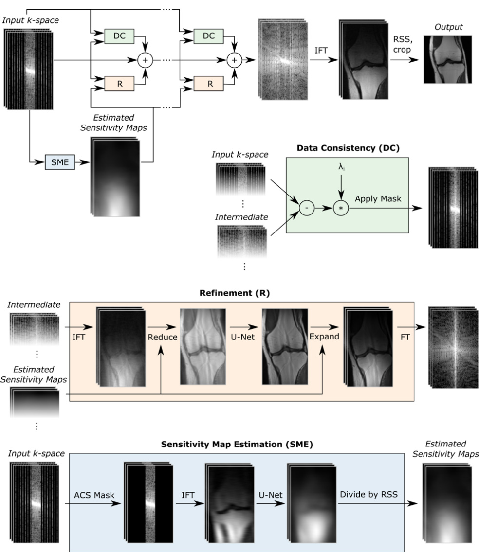
Fig. 1: Top: Block diagram of our model which takes under-sampled $\mathrm{k}$ -space as input and applies several cascades, followed by an inverse Fourier transform (IFT) and an RSS transform. The Data Consistency (DC) module computes a correction map that brings the intermediate k-space closer to the measured k-space values. The Refinement (R) module maps multi-coil k-space data into one image, applies a U-Net, and then back to multi-coil k-space data. The Sensitivity Map Estimation (SME) module estimates the sensitivity maps used in the Refinement module.

图 1: 上: 我们的模型框图，以欠采样的 $\mathrm{k}$ 空间作为输入，应用多个级联模块，随后进行逆傅里叶变换 (IFT) 和 RSS 变换。数据一致性 (DC) 模块计算校正图，使中间 k 空间更接近测量的 k 空间值。细化 (R) 模块将多线圈 k 空间数据映射为一张图像，应用 U-Net，然后返回多线圈 k 空间数据。灵敏度图估计 (SME) 模块估计用于细化模块的灵敏度图。

3.3 Learned sensitivity maps

3.3 学习得到的敏感度图

The expand and reduce operators in equation 11 take sensitivity maps $(S_{1},...,S_{N})$ as inputs. In the original VarNet model, these sensitivity maps are computed using the ESPIRiT algorithm [15] and fed in to the model as additional inputs. In our model, however, we estimate the sensitivity maps as part of the reconstruction network using a Sensitivity Map Estimation (SME) module:

方程11中的扩展和缩减操作以灵敏度图$(S_{1},...,S_{N})$作为输入。在原始VarNet模型中，这些灵敏度图使用ESPIRiT算法[15]计算，并作为额外输入馈入模型。然而，在我们的模型中，我们通过灵敏度图估计(Sensitivity Map Estimation, SME)模块将灵敏度图估计作为重建网络的一部分。

$$
H=\mathrm{d}\mathrm{S}\mathrm{S}\circ\mathrm{C}\mathrm{N}\mathrm{N}\circ\mathcal{F}^{-1}\circ M_{\mathrm{center}}.
$$

$$
H=\mathrm{d}\mathrm{S}\mathrm{S}\circ\mathrm{C}\mathrm{N}\mathrm{N}\circ\mathcal{F}^{-1}\circ M_{\mathrm{center}}.
$$

The $M_{\mathrm{center}}$ operator zeros out all lines except for the auto calibration or ACS lines (described in Section 2.1). This is similar to classical parallel imaging approaches which estimate sensitivity maps from the ACS lines. The CNN follows the same architecture as the CNN in the cascades, except with fewer channels and thus fewer parameters in intermediate layers. This CNN is applied to each coil image independently. Finally, the dSS operator normalizes the estimated sensitivity maps to ensure that the property in equation 3 is satisfied.

$M_{\mathrm{center}}$ 运算符会清零除自动校准线或 ACS 线 (详见第 2.1 节) 外的所有线。这与传统并行成像方法类似，后者通过 ACS 线估算灵敏度图。该 CNN 采用与级联结构中 CNN 相同的架构，但通道数更少，因此中间层的参数也更少。该 CNN 会独立应用于每个线圈图像。最后，dSS 运算符会对估算的灵敏度图进行归一化处理，以确保满足公式 3 中的特性。

3.4 E2E-VarNet model architecture

3.4 E2E-VarNet 模型架构

As previously described, our model takes the masked multi-coil k-space $\mathbf{k}{0}$ as input. First, we apply the SME module to $\mathbf{k}_{0}$ to compute the sensitivity maps. Next we apply a series of cascades, each of which applies the function in equation 10, to the input k-space to obtain the final k-space representation $K^{T}$ . This final k-space representation is converted to image space by applying an inverse Fourier transform followed by a root-sum-squares (RSS) reduction for each pixel:

如前所述，我们的模型以掩膜多线圈k空间$\mathbf{k}{0}$作为输入。首先，我们对$\mathbf{k}_{0}$应用SME模块来计算灵敏度图。接着，我们对输入k空间应用一系列级联操作（每个级联都执行公式10中的函数）以获得最终的k空间表示$K^{T}$。最后通过逆傅里叶变换及逐像素的平方和根(RSS)压缩，将该k空间表示转换到图像空间：

$$
\hat{\mathbf{x}}=R S S(\mathbf{x}{1},...,\mathbf{x}{N})=\sqrt{\sum_{i=1}^{N}|\mathbf{x}_{i}|^{2}}
$$

$$
\hat{\mathbf{x}}=R S S(\mathbf{x}{1},...,\mathbf{x}{N})=\sqrt{\sum_{i=1}^{N}|\mathbf{x}_{i}|^{2}}
$$

where $\mathbf{x}{i}=\mathcal{F}^{-1}(K_{i}^{T})$ and $K_{i}^{T}$ is the $\mathrm{k\Omega}$ -space representation for coil $i$ . The model is illustrated in figure 1.

其中 $\mathbf{x}{i}=\mathcal{F}^{-1}(K_{i}^{T})$ ，且 $K_{i}^{T}$ 是线圈 $i$ 的 $\mathrm{k\Omega}$ 空间表示。该模型如图 1 所示。

All of the parameters of the network, including the parameters of the CNN model in SME, the parameters of the CNN in each cascade along with the $\eta^{t_{\mathrm{i}}}$ s, are estimated from the training data by minimizing the structural similarity loss, $J(\hat{\mathbf{x}},\mathbf{x}^{})=-\operatorname{SSIM}(\hat{\mathbf{x}},\mathbf{x}^{})$ , where SSIM is the Structural Similarity index [16] and $\hat{\bf x}$ , $\mathbf{x}^{*}$ are the reconstruction and ground truth images, respectively.

网络的所有参数，包括SME中CNN模型的参数、每个级联中CNN的参数以及$\eta^{t_{\mathrm{i}}}$，均通过最小化结构相似性损失$J(\hat{\mathbf{x}},\mathbf{x}^{})=-\operatorname{SSIM}(\hat{\mathbf{x}},\mathbf{x}^{})$从训练数据中估计得出。其中SSIM为结构相似性指数[16]，$\hat{\bf x}$和$\mathbf{x}^{*}$分别表示重建图像和真实图像。

4 Experiments

4 实验

4.1 Experimental setup

4.1 实验设置

We designed and validated our method using the multicoil track of the fastMRI dataset [18] which is a large and open dataset of knee and brain MRIs. To validate the various design choices we made, we evaluated the following models on the knee dataset:

我们使用fastMRI数据集[18]的多线圈轨迹设计和验证了我们的方法，这是一个大型开放的膝部和脑部MRI数据集。为了验证我们所做的各种设计选择，我们在膝部数据集上评估了以下模型：

The VN model employs shallow convolutional networks with RBF kernels that have about 150K parameters in total. VNU replaces these shallow networks with U-Nets to ensure a fair comparison with our model. VNU-K is similar to our proposed model but uses fixed sensitivity maps computed using classical parallel imaging methods. The difference in reconstruction quality between VNU and VNU-K shows the value of using k-space intermediate quantities for reconstruction, while the difference between VNU-K and E2E-VN shows the importance of learning sensitivity maps as part of the network.

VN模型采用具有RBF核的浅层卷积网络，总参数量约为15万。VNU将这些浅层网络替换为U-Nets，以确保与我们的模型进行公平比较。VNU-K与我们提出的模型类似，但使用了通过经典并行成像方法计算的固定灵敏度图。VNU与VNU-K在重建质量上的差异体现了使用k空间中间量进行重建的价值，而VNU-K与E2E-VN的差异则表明将灵敏度图作为网络一部分进行学习的重要性。

We used the same model architecture and training procedure for the VN model as in the original VarNet [4] paper. For each of the other models, we used $T=12$ cascades, containing a total of about 29.5M parameters. The E2E-VN model contained an additional 0.5M parameters in the SME module, taking the total number of parameters to 30M. We trained these models using the Adam optimizer with a learning rate of 0.0003 for 50 epochs, without using any regular iz ation or data augmentation techniques.

我们为VN模型采用了与原始VarNet [4]论文相同的模型架构和训练流程。其他各模型均使用$T=12$级联结构，总计约29.5M参数。E2E-VN模型在SME模块中额外包含0.5M参数，使总参数量达到30M。所有模型均采用Adam优化器（学习率0.0003）训练50个周期，未使用任何正则化或数据增强技术。

We used two types of under-sampling masks: equispaced masks $M_{e}(r,l)$ , which sample $\textit{l}$ low-frequency lines from the center of k-space and every $r$ -th line from the remaining k-space; and random masks $M_{r}(a,f)$ , which sample a fraction $f$ of the full width of k-space for the ACS lines in addition to a subset of higher frequency lines, selected uniformly at random, to make the overall acceleration equal to $a$ . These random masks are identical to those used in [18]. We also use equispaced masks as they are easier to implement in MRI machines.

我们使用了两种类型的欠采样掩码：等间距掩码 $M_{e}(r,l)$ ，它从k空间中心采样 $\textit{l}$ 条低频线，并从剩余的k空间中每隔 $r$ 条线采样一条；以及随机掩码 $M_{r}(a,f)$ ，除了随机均匀选择的高频线子集外，还对k空间全宽的 $f$ 部分进行采样以采集自动校准信号 (ACS) 线，使整体加速因子等于 $a$ 。这些随机掩码与[18]中使用的相同。我们也采用等间距掩码，因为它们更易于在MRI机器上实现。

Fig. 2: Examples comparing the ground truth (GT) to VarNet (VN) and E2E-VarNet (E2E-VN). At $8\times$ acceleration, the VN images contain severe artifacts.

图 2: 真实数据 (GT) 与 VarNet (VN) 和 E2E-VarNet (E2E-VN) 的对比示例。在 $8\times$ 加速条件下，VN 图像存在严重伪影。

4.2 Results

4.2 结果

Tables 1 and 2 show the results of our experiments for equispaced and random masks respectively, over a range of down-sampling mask parameters. The VNU model outperforms the baseline VN model by a large margin due to its larger capacity and the multi-scale modeling ability of the U-Nets. VNU-K outperforms VNU demonstrating the value of using k-space intermediate quantities. E2E-VN outperforms VNU-K showing the importance of learning sensitivity maps as part of the network. It is worth noting that the relative performance does not depend on the type of mask or the mask parameters. Some example reconstructions are shown in figure 2.

表1和表2分别展示了等间距掩膜和随机掩膜在不同降采样掩膜参数下的实验结果。得益于更大的容量和U-Net的多尺度建模能力，VNU模型显著优于基准VN模型。VNU-K优于VNU，证明了使用k空间中间量的价值。E2E-VN优于VNU-K，表明将灵敏度图学习作为网络组成部分的重要性。值得注意的是，相对性能与掩膜类型或掩膜参数无关。图2展示了一些重建示例。

Significance of learning sensitivity maps Figure 3 shows the SSIM values for each model with various equispaced mask parameters. In all cases, learning the sensitivity maps improves the SSIM score. Notably, this improvement in SSIM is larger when the number of low frequency lines is smaller. As previously stated, the quality of the estimated sensitivity maps tends to be poor when there are few ACS lines, which leads to a degradation in the final reconstruction quality. The E2E-VN model is able to overcome this limitation and generate good reconstructions even with a small number of ACS lines.

学习灵敏度图的重要性
图 3 展示了不同等间距掩码参数下各模型的 SSIM 值。在所有情况下，学习灵敏度图都能提高 SSIM 分数。值得注意的是，当低频线数量较少时，SSIM 的提升更为明显。如前所述，当 ACS 线较少时，估计的灵敏度图质量往往较差，这会导致最终重建质量下降。E2E-VN 模型能够克服这一限制，即使 ACS 线数量较少也能生成良好的重建结果。

Accel(r) Num ACS(l) Model	SSIM
4 30	VN VNU
	VNU-K
6	E2E-VN VN
	22 VNU
	VNU-K
	E2E-VN
8	16
	VNU-K

Accel(a) Frac ACS(f) 模型	SSIM
4	VN
	0.08 VNU
	VNU-K E2E-VN(
6	VN
	0.06 VNU
	VNU-K E2E-VN(
8	0.04 E2E-VN0.878
	VNU VNU-K

Fig. 3: Effect of different equispaced mask parameters on reconstruction quality at $4\times$ and $6\times$ acceleration. Table 1: Experimental results using equispaced masks on the knee MRIs Table 2: Experimental results using random masks on the knee MRIs

图 3: 不同等间距掩码参数在 $4\times$ 和 $6\times$ 加速倍数下对重建质量的影响
表 1: 膝关节 MRI 使用等间距掩码的实验结果
表 2: 膝关节 MRI 使用随机掩码的实验结果

Experiments on test data Table 3 shows our results on the test datasets for both the brain and knee MRIs compared with the best models on the fastMRI leader board 4. To obtain these results, we used the same training procedure as our previous experiments, except that we trained on both the training and validation sets for 100 epochs. We used the same type of masks that are used for the fastMRI paper [4]. Our model outperforms all other models published on the fastMRI leader board for both anatomies.

测试数据实验
表3展示了我们在脑部和膝盖MRI测试数据集上的结果，与fastMRI排行榜上最佳模型的对比[4]。为获得这些结果，我们采用了与先前实验相同的训练流程，唯一区别是将训练集和验证集共同训练了100个周期。我们使用了与fastMRI论文[4]相同类型的掩模。对于两种解剖部位，我们的模型均超越了fastMRI排行榜上发布的所有其他模型。

5 Conclusion

5 结论

In this paper, we introduced End-to-End Variation al Networks for multi-coil MRI reconstruction. While MRI reconstruction can be posed as an inverse problem, multi-coil MRI reconstruction is particularly challenging because the forward process (which is determined by the sensitivity maps) is not completely known. We alleviate this problem by estimating the sensitivity maps within the network, and learning fully end-to-end. Further, we explored the architecture space to identify the best neural network layers and intermediate representation for this problem, which allowed our model to obtain new state-of-the art results on both brain and knee MRIs.

本文介绍了用于多线圈MRI重建的端到端变分网络。虽然MRI重建可以被视为一个逆问题，但多线圈MRI重建尤其具有挑战性，因为前向过程（由灵敏度图决定）并非完全已知。我们通过在网络内部估计灵敏度图并实现完全端到端学习来缓解这一问题。此外，我们探索了架构空间以确定最适合该问题的神经网络层和中间表示，这使得我们的模型在脑部和膝部MRI上都获得了新的最先进结果。

Table 3: Results on the test data compared with the best models on the fastMRI leader board

表 3: 测试数据结果与fastMRI排行榜最佳模型对比

数据集	模型	4倍加速		8倍加速
		SSIM	NMSE PSNR	SSIM	NMSE	PSNR
Knee	E2E-VN	0.930 0.005	40	0.890	0.009	37
	SubtleMR	0.929 0.005	40	0.888	0.009	37
	AIRSMedical	0.929 0.005	40	0.888	0.009	37
	SigmaNet	0.928 0.005	40	0.888	0.009	37
	i-RIM	0.928 0.005	40	0.888	0.009	37
Brain	E2E-VN	0.959 0.004	41	0.943	0.008	38
	U-Net	0.945 0.011	38	0.915	0.023	35

The quantitative measures we have used only provide a rough estimate for the quality of the reconstructions. Many clinically important details tend to be subtle and limited to small regions of the MR image. Rigorous clinical validation needs to be performed before such methods can be used in clinical practice to ensure that there is no degradation in the quality of diagnosis.

我们采用的定量测量方法仅能对重建质量提供粗略估计。许多临床关键细节往往较为细微，且局限于磁共振图像的小范围区域。在将这些方法应用于临床实践之前，必须进行严格的临床验证，以确保诊断质量不会下降。

Bibliography

参考文献

6 Supplementary Materials

6 补充材料

6.1 Dithering as post-processing

6.1 作为后处理的抖动 (Dithering)

The Structural Similarity (SSIM) loss [17] we used to train our models has a tendency to produce overly smooth reconstructions even when all of the diagnostic content is preserved. We noticed a similar behavior with other frequently used loss functions like mean squared error, mean absolute error, etc. Sriram et al. [14] found that dithering the image by adding a small amount of random gaussian noise helped enhance the perceived sharpness of their reconstructions. We found that the same kind of dithering helped improve the sharpness of our reconstructions, but we tuned the scale of the noise by manual inspection.

我们用于训练模型的结构相似性 (SSIM) 损失 [17] 倾向于产生过度平滑的重建结果，即使所有诊断内容都得到保留。在使用其他常用损失函数（如均方误差、平均绝对误差等）时，我们也观察到了类似现象。Sriram 等人 [14] 发现，通过添加少量随机高斯噪声对图像进行抖动处理，有助于提升重建结果的感知锐度。我们发现同类抖动方法也能改善我们重建结果的锐度，但通过人工观察调整了噪声的幅度。

Similar to [14], we adjusted the scale of the added noise to the brightness of the image around each pixel to avoid obscuring dark areas of the reconstruction. Specifically, we first normalize the image by dividing each pixel by the maximum pixel intensity. Then we add zero-mean random gaussian noise to each pixel. The standard deviation of the noise at a given pixel location is equal to $\sigma$ times the square root of the local median computed over a patch of $11\times11$ pixels around that pixel location. We set $\sigma=0.02$ for the brain images and non fat suppressed knee images, and $\sigma=0.03$ for the fat suppressed knee images.

与[14]类似，我们根据每个像素周围图像的亮度调整添加噪声的幅度，以避免掩盖重建图像中的暗部区域。具体而言，首先通过将每个像素除以最大像素强度对图像进行归一化处理，然后为每个像素添加零均值随机高斯噪声。给定像素位置的噪声标准差等于 $\sigma$ 乘以该像素位置周围 $11\times11$ 像素区域内局部中位数的平方根。对于脑部图像和非脂肪抑制膝关节图像，我们设定 $\sigma=0.02$；对于脂肪抑制膝关节图像，设定 $\sigma=0.03$。

Example reconstructions with and without noise are shown in figs. 4 to 7. The dithered images look more natural, especially at higher accelerations.

图4至图7展示了带噪声和无噪声的示例重建结果。经过抖动的图像看起来更自然，尤其在更高加速比的情况下。

Fig. 4: Brain images showing ground truth (left), reconstruction (middle) and reconstruction with added noise (right) at $4\times$ acceleration

图 4: 展示真实情况(左)、重建图像(中)及添加噪声后重建图像(右)的脑部影像 (4倍加速)

Fig. 5: Brain images showing ground truth (left), reconstruction (middle) and reconstruction with added noise (right) at 8 $\times$ acceleration

图 5: 展示8倍加速下的真实脑部图像 (左)、重建图像 (中) 及添加噪声后的重建图像 (右)

Fig. 6: Knee images showing ground truth (left), reconstruction (middle) and reconstruction with added noise (right) at $4\times$ acceleration

图 6: 膝关节图像展示真实情况 (左)、重建结果 (中) 以及添加噪声后的重建结果 (右)，加速比为 $4\times$

Fig. 7: Knee images showing ground truth (left), reconstruction (middle) and reconstruction with added noise (right) at 8 $\times$ acceleration

图 7: 膝关节图像展示8倍加速下的真实情况(左)、重建结果(中)及添加噪声后的重建结果(右)