Unsupervised Pre-Training on Patient Population Graphs for Patient-Level Predictions
基于患者群体图的无监督预训练在患者级别预测中的应用
Abstract. Pre-training has shown success in different areas of machine learning, such as Computer Vision (CV), Natural Language Processing (NLP) and medical imaging. However, it has not been fully explored for clinical data analysis. Even though an immense amount of Electronic Health Record (EHR) data is recorded, data and labels can be scarce if the data is collected in small hospitals or deals with rare diseases. In such scenarios, pre-training on a larger set of EHR data could improve the model performance. In this paper, we apply unsupervised pre-training to heterogeneous, multi-modal EHR data for patient outcome prediction. To model this data, we leverage graph deep learning over population graphs. We first design a network architecture based on graph transformer designed to handle various input feature types occurring in EHR data, like continuous, discrete, and time-series features, allowing better multi-modal data fusion. Further, we design pre-training methods based on masked imputation to pre-train our network before fine-tuning on different end tasks. Pre-training is done in a fully unsupervised fashion, which lays the groundwork for pre-training on large public datasets with different tasks and similar modalities in the future. We test our method on two medical datasets of patient records, TADPOLE and MIMIC-III, including imaging and non-imaging features and different prediction tasks. We find that our proposed graph based pretraining method helps in modeling the data at a population level and further improves performance on the fine tuning tasks in terms of AUC on average by $4.15%$ for MIMIC and $7.64%$ for TADPOLE.
摘要。预训练已在机器学习的不同领域展现出成效,如计算机视觉(CV)、自然语言处理(NLP)和医学影像。然而,其在临床数据分析中的应用尚未得到充分探索。尽管电子健康记录(EHR)数据被大量记录,但如果数据来自小型医院或涉及罕见疾病,数据和标签可能仍然稀缺。在此类场景中,基于更大规模EHR数据的预训练有望提升模型性能。本文针对异质多模态EHR数据,采用无监督预训练方法进行患者预后预测。为建模此类数据,我们利用基于群体图的图深度学习技术。首先设计了一种基于图Transformer的网络架构,可处理EHR数据中各类输入特征类型(如连续型、离散型和时序特征),实现更优的多模态数据融合;其次设计了基于掩码填补的预训练方法,用于在不同下游任务微调前预训练网络。预训练全程采用无监督方式,为未来在大型公共数据集上开展跨任务、同模态预训练奠定基础。我们在TADPOLE和MIMIC-III两个包含影像与非影像特征的患者记录医疗数据集上测试方法,涉及不同预测任务。实验表明,基于图的预训练方法能有效建模群体层面数据,使微调任务平均AUC指标提升:MIMIC提升4.15%,TADPOLE提升7.64%。
1 Introduction
1 引言
Enormous amounts of data are collected on a daily basis in hospitals. Nevertheless, labeled data can be scarce, as labeling can be tedious, time-consuming, and expensive. Further, in small hospitals and for rare diseases, only little data is accumulated [15]. The ability to leverage the large body of unlabeled medical data to improve in prediction tasks over such small labeled datasets could increase the confidence of AI models for clinical outcome prediction. Unsupervised pre-training was shown to be useful to exploit unlabeled data in NLP [20,4],
医院每天都会收集大量数据。然而,标注数据可能十分稀缺,因为标注过程往往繁琐、耗时且成本高昂。此外,小型医院和罕见疾病领域积累的数据量通常有限 [15]。若能利用海量未标注医疗数据来提升小规模标注数据集上的预测任务性能,将显著增强AI模型在临床结果预测中的可信度。无监督预训练已被证明能有效挖掘NLP领域未标注数据的价值 [20,4]。
CV [18,1] and medical imaging [16,2]. However, for more complex clinical data, it is not explored enough. Some works study how to pre-train BERT [4] over EHR data of medical diagnostic codes. They pre-train with modified masked language modeling and, in one case, a supervised prediction task. The targeted downstream tasks lie in disease and medication code prediction [23,11,21]. McDermott et al. [14] propose a pre-training approach over heterogeneous EHR data, including e.g. continuous lab results. They create a benchmark with several downstream tasks over the eICU [19] and MIMIC-III [7] datasets and present two baseline pre-training methods. Pre-training and fine-tuning are performed over single EHRs from ICU stays with a Gated Recurrent Unit.
计算机视觉 [18,1] 和医学影像 [16,2] 领域已有相关研究。然而,针对更复杂的临床数据,探索仍显不足。部分研究探讨了如何在医疗诊断编码的电子健康记录 (EHR) 数据上预训练 BERT [4],采用改进的掩码语言建模方法进行预训练,其中一项研究还结合了监督预测任务。这些研究的下游任务目标集中在疾病和药物编码预测 [23,11,21]。McDermott 等人 [14] 提出了一种针对异构 EHR 数据(包括连续实验室结果等)的预训练方法。他们基于 eICU [19] 和 MIMIC-III [7] 数据集创建了包含多个下游任务的基准测试,并提出了两种基线预训练方法。该方法使用门控循环单元 (Gated Recurrent Unit) 对 ICU 住院期间的单一 EHR 数据进行预训练和微调。
On the other hand, population graphs have been leveraged in the recent literature to help analyze patient data using the relationships among patients, leading to clinically semantic modeling of the data. During unsupervised pre-training, graphs allow learning representations based on feature similarities between the patients, which can then help to improve patient-level predictions. Several works successfully apply pre-training to graph data in different domains like molecular graphs and on common graph benchmarks. Proposed pre-training strategies include node level tasks, like attribute reconstruction, graph level tasks like property prediction, or generative tasks such as edge prediction [5,22,27,6,12]. To the best of our knowledge, no previous work applied pre-training to population graphs.
另一方面,近期研究利用人群图 (population graphs) 通过患者间的关系辅助分析临床数据,实现对数据的临床语义建模。在无监督预训练阶段,图结构能基于患者间的特征相似性学习表征,从而提升患者层面的预测效果。多项研究已成功将预训练应用于分子图等不同领域的图数据及常见图基准测试。提出的预训练策略包括节点级任务(如属性重构)、图级任务(如性质预测)以及生成式任务(如边预测)[5,22,27,6,12]。据我们所知,尚无研究将预训练应用于人群图。
In this paper, we propose a model capable of pre-training for understanding patient population data. We choose two medical applications in brain imaging and EHR data analysis on the public datasets TADPOLE [13] and MIMICIII [7] for Alzheimer’s disease prediction [17,9,3] and Length-of-Stay prediction [26,24,14]. The code is available at https://github.com/ChantalMP/UnsupervisedPre-Training-on-Patient-Population-Graphs-for-Patient-Level-Predictions.
本文提出了一种能够预训练以理解患者群体数据的模型。我们在公共数据集TADPOLE [13]和MIMICIII [7]上选择了脑成像和电子健康记录(EHR)数据分析两个医疗应用,分别用于阿尔茨海默病预测[17,9,3]和住院时长预测[26,24,14]。代码可在https://github.com/ChantalMP/UnsupervisedPre-Training-on-Patient-Population-Graphs-for-Patient-Level-Predictions获取。
Contribution: We develop an unsupervised pre-training method to learn a general understanding of patient population data modeled as graph, providing a solution to limited labeled data. We show significant performance gains through pre-training when fine-tuning with as little as $1%$ and up to $100%$ labels. Further, we propose a (graph) transformer based model suitable for multi-modal data fusion. It is designed to handle various EHR input types, taking static and time-series data and continuous as well as discrete numerical features into account.
贡献:我们开发了一种无监督预训练方法,用于学习以图结构建模的患者群体数据的通用理解,为解决标注数据有限的问题提供了方案。实验表明,在使用少至1%到多达100%的标注数据进行微调时,预训练能带来显著的性能提升。此外,我们提出了一种基于Transformer的模型,适用于多模态数据融合。该模型设计用于处理各类电子健康记录(EHR)输入,同时考虑静态与时序数据、连续及离散数值特征。
2 Method
2 方法
Let $\mathbf{D}$ be a dataset composed of the EHR data of $N$ patients. The $i^{t h}$ record is represented by $\mathbf{r_{i}}\subseteq[\mathbf{d_{i}},\mathbf{c_{i}},\mathbf{t_{i}}]$ with static discrete features $\mathbf{d}{\mathbf{i}}\in\mathbb{N}^{D}$ , continuous features $\mathbf{c_{i}}\in\mathbb{R}^{C}$ , and time-series features $\mathbf{t_{i}}\in\mathbb{R}^{S\times\tau}$ , where $\tau$ denotes the length of the time-series. For every downstream task $T$ , labels $\mathbf{Y}\in\mathbb{N}^{L}$ are given for $\mathrm{L}$ classes. The task is to predict the classes for the test set patients given all features. Towards this task, we propose to use patient population graphs. Unlike in non-graph-based methods, the model can exploit similarities between patients to better understand the EHR data at patient and population level. Further, unlike conventional graph neural networks, graph transformers allow flexible attention to all nodes, learning which patients are relevant for a task. This would be most apt for learning over population EHR data. Our pipeline consists of two steps. 1) Unsupervised pre-training and 2) Fine-tuning. Unsupervised pre-training enables understanding of general EHR data and disorder progression by training the model for masked imputation task. This understanding can help learn downstream tasks better despite limited labeled data.
设 $\mathbf{D}$ 为一个由 $N$ 名患者的电子健康记录(EHR)数据组成的数据集。第 $i^{t h}$ 条记录表示为 $\mathbf{r_{i}}\subseteq[\mathbf{d_{i}},\mathbf{c_{i}},\mathbf{t_{i}}]$,其中包含静态离散特征 $\mathbf{d}{\mathbf{i}}\in\mathbb{N}^{D}$、连续特征 $\mathbf{c_{i}}\in\mathbb{R}^{C}$ 以及时间序列特征 $\mathbf{t_{i}}\in\mathbb{R}^{S\times\tau}$,其中 $\tau$ 表示时间序列的长度。对于每个下游任务 $T$,给定 $\mathrm{L}$ 个类别的标签 $\mathbf{Y}\in\mathbb{N}^{L}$。该任务的目标是根据所有特征预测测试集患者的类别。为此,我们提出使用患者群体图。与非基于图的方法不同,该模型可以利用患者之间的相似性,更好地在患者和群体层面理解EHR数据。此外,与传统图神经网络不同,图Transformer可以灵活关注所有节点,学习哪些患者与任务相关。这最适合于基于群体EHR数据的学习。我们的流程包含两个步骤:1) 无监督预训练;2) 微调。无监督预训练通过训练模型完成掩码填补任务,实现对EHR数据和疾病进展的一般性理解。这种理解有助于在标记数据有限的情况下更好地学习下游任务。
Graph Construction For each node pair with records $r_{i}$ and $r_{j}$ , we calculate a similarity score $S(r_{i},r_{j})$ between the node features. We use L2 distance for continuous and absolute matching for discrete features. As graph construction is not our focus, we choose the most conventional method using k-NN selection rule. We set k=5 to avoid having many disconnected components and very densely connected regions (see supplementary material). A detailed description of the graph construction per dataset follows in the experiment section.
图构建 对于每对包含记录$r_{i}$和$r_{j}$的节点,我们计算节点特征之间的相似度得分$S(r_{i},r_{j})$。连续特征采用L2距离,离散特征采用精确匹配。由于图构建并非本文重点,我们选用最常规的k近邻(k-NN)选择规则,设定k=5以避免产生过多不连通组件和过度稠密连接区域(详见补充材料)。各数据集的具体图构建方法将在实验部分详述。
Model Architecture Our model consists of an encoder and decoder. The encoder comprises a data embedding module and a graph transformer module explained later. We design the encoder to handle various input data types. The decoder is a simple linear layer capable of capturing the essence of features inclined towards a node-level classification task. Figure 1 shows an overview of our model architecture.
模型架构
我们的模型由编码器和解码器组成。编码器包含数据嵌入模块和后续介绍的图Transformer模块。我们设计的编码器能够处理多种输入数据类型。解码器是一个简单的线性层,能够捕捉偏向节点级分类任务的特征本质。图1展示了我们模型架构的概览。
Data embedding module: Following the conventional Graphormer [25], we process discrete input features by an embedding layer, followed by a summation over the feature dimension, resulting in embedded features $\mathbf{d}{\mathbf{i}}^{\prime}\in\mathbb{R}^{D^{\prime}}$ , where $D^{\prime}$ is the output feature dimension. While Graphormer is limited to static, discrete input features only, we improve upon Graphormer to support also static, continuous input features, which are processed by a linear layer resulting in the embedding vector $\mathbf{c_{i}^{\prime}}\in\mathbb{R}^{C^{\prime}}$ . The third branch of our data embedding module handles timeseries input features $\mathbf{t_{i}}\in\mathbb{R}^{S\times\tau}$ with a linear layer, followed by two transformer layers to deal with variable sequence lengths and allow the model to incorporate temporal context. The output is given by $\mathbf{t}{\mathbf{i},\mathbf{h}}^{\prime}\in\mathbb{R}^{E}$ per time-step h. The mean of these embeddings forms the final time-series embeddings $\mathbf{t}{\mathbf{i}}^{\prime}\in\mathbb{R}^{S^{\prime}}$ . The feature vectors $\mathbf{d_{i}^{\prime},c_{i}^{\prime}}$ and $\mathbf{t_{i}^{\prime}}$ are concatenated to form the final node embeddings $n_{i}\in\mathbb{R}^{F}$ , where $\begin{array}{r}{\boldsymbol{F}=\sum_{F_{k}\subset[D^{\prime},C^{\prime},S^{\prime}]}F_{k}}\end{array}$ , for each of the $N$ nodes.
数据嵌入模块:遵循传统Graphormer [25]的做法,我们通过嵌入层处理离散输入特征,随后沿特征维度求和得到嵌入特征$\mathbf{d}{\mathbf{i}}^{\prime}\in\mathbb{R}^{D^{\prime}}$,其中$D^{\prime}$为输出特征维度。Graphormer仅支持静态离散输入特征,我们在此基础上改进以支持静态连续输入特征,这类特征通过线性层处理生成嵌入向量$\mathbf{c_{i}^{\prime}}\in\mathbb{R}^{C^{\prime}}$。该模块的第三分支通过线性层处理时序输入特征$\mathbf{t_{i}}\in\mathbb{R}^{S\times\tau}$,再经两个Transformer层处理可变序列长度并融入时序上下文信息,最终输出每个时间步h的$\mathbf{t}{\mathbf{i},\mathbf{h}}^{\prime}\in\mathbb{R}^{E}$。这些嵌入的均值构成最终时序嵌入$\mathbf{t}{\mathbf{i}}^{\prime}\in\mathbb{R}^{S^{\prime}}$。将特征向量$\mathbf{d_{i}^{\prime},c_{i}^{\prime}}$与$\mathbf{t_{i}^{\prime}}$拼接后形成最终节点嵌入$n_{i}\in\mathbb{R}^{F}}$,其中$\begin{array}{r}{\boldsymbol{F}=\sum_{F_{k}\subset[D^{\prime},C^{\prime},S^{\prime}]}F_{k}}\end{array}$,共生成$N$个节点的嵌入。
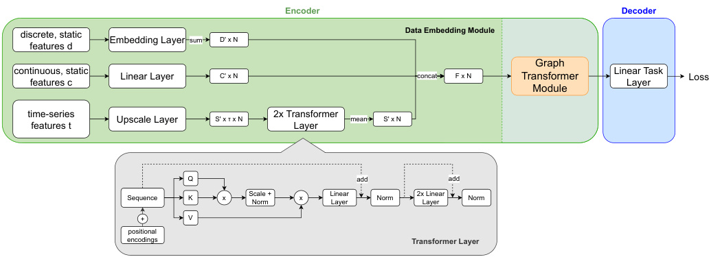
Fig. 1. Overview of the proposed architecture. All input features are combined into one node embedding, applying transformer layers to enhance the time-series features. The upscale layer for time-series features is a linear layer for continuous and an embedding layer followed by a summation over the feature dimension for discrete features. The resulting graph is processed by several Graphormer layers and a linear task layer.
图 1: 提出的架构概览。所有输入特征被合并为一个节点嵌入 (node embedding),应用 Transformer 层来增强时间序列特征。时间序列特征的上采样层对连续特征采用线性层,对离散特征采用嵌入层后沿特征维度求和。生成的图会经过多个 Graphormer 层和一个线性任务层的处理。
Graphormer Module: The backbone of our model comprises multiple graph transformer layers [25]. Graphormer uses attention between all nodes in the graph. To incorporate the graph structure, structural encodings are used, which encode in and out degrees of the nodes, the distance between nodes, and edge features. Pre-training and Fine-Tuning: We propose an unsupervised pre-training technique on the same input features as for downstream tasks, but without using labels $\mathbf{Y}$ . Instead, we randomly mask a fixed percentage of feature values for every record $\mathbf{r_{i}}$ and optimize the model to predict these values. For all methods masking is performed by replacing certain feature values with a fixed value called ’masked token’ for discrete features and with zero for continuous features. For time-series features, we further add a binary column per feature to the input vector, that encodes which hours in the time-series are masked. We optimize the model using (binary) cross entropy loss for discrete and mean squared error loss for continuous features. A model for fine-tuning is initialized using the encoder weights learned during pre-training and random weights for the decoder. Then the model is fine-tuned for the task $T$ .
Graphormer模块:
我们的模型主干由多个图Transformer层[25]构成。Graphormer通过计算图中所有节点间的注意力机制运作。为融入图结构信息,模型采用结构编码技术,对节点的入度/出度、节点间距离及边特征进行编码。
预训练与微调:
我们提出一种无监督预训练技术,其输入特征与下游任务相同,但不使用标签$\mathbf{Y}$。具体实现时,对每条记录$\mathbf{r_{i}}$随机遮蔽固定比例的特征值,并通过模型预测这些值来优化参数。所有方法均采用固定值(离散特征用"遮蔽token",连续特征用零值)替换被遮蔽特征。针对时序特征,我们还在输入向量中为每个特征添加二元列,用于标记被遮蔽的时间点。模型优化时,离散特征采用(二元)交叉熵损失函数,连续特征采用均方误差损失函数。微调模型时,编码器使用预训练获得的权重初始化,解码器则采用随机权重,随后针对任务$T$进行微调。
3 Experiments and Results
3 实验与结果
We use two publicly available medical data sets: TADPOLE [13] and MIMICIII [7]. They differ in size, the targeted prediction task, and the type of input features, allowing comprehensive testing and evaluation of our method.
我们使用了两个公开可用的医学数据集:TADPOLE [13] 和 MIMICIII [7]。它们在数据规模、预测任务目标和输入特征类型上存在差异,能够全面测试和评估我们的方法。
3.1 Datasets description:
3.1 数据集描述:
TADPOLE [13] contains 564 patients from the Alzheimer’s Disease Neuroimaging Initiative (ADNI). We use twelve features, which the TADPOLE challenge claims are informative. They include discrete cognitive test results, demographics, and continuous features extracted from MR and PET imaging, normalized between zero and one. The task is to classify the patients into the groups Cognitive Normal (CN), Mild Cognitive Impairment (MCI), or Alzheimer’s Disease (AD). We only use data from patients’ first visits to avoid leakage of information. Graph Construction: We construct a k-NN graph with k=5, dependent on the mean similarity ( $S$ ) between the features. For the demographics, age, gender and if $f_{i}=f_{j}$ else 0 apoe4, if $|a g e_{i}-a g e_{j}|\leq2$ else 0 $\div3$ where, $f$ =(apoe4, gender). For the cognitive test results $\mathbf{d}{\mathbf{i}}$ (ordinal features), and $\mathbf{c_{i}}$ (continuous imaging features), we calculate the respective normalized L2 distances: $\begin{array}{r}{S_{c o g}(r_{i},r_{j})=\frac{\sum_{f\in\mathbf{d_{i}}}\vert\vert f_{r_{i}}-f_{r_{j}}\vert\vert}{m a x(\mathbf{d_{i}})}}\end{array}$ and $\begin{array}{r}{S_{i m g}(r_{i},r_{j})=s i g(\sum_{f\in\mathbf{c_{i}}}||f_{r_{i}}-f_{r_{j}}||)}\end{array}$ . The overall similarity $S(r_{i},r_{j})$ is then given as mean of $S_{d e m}$ , $S_{c o g}$ and $S_{i m g}$ .
TADPOLE [13] 数据集包含来自阿尔茨海默病神经影像计划 (ADNI) 的564名患者。我们使用了TADPOLE挑战赛声称具有信息量的12个特征,包括离散认知测试结果、人口统计学数据,以及从MR和PET成像中提取并归一化到0到1之间的连续特征。任务是将患者分类为认知正常 (CN)、轻度认知障碍 (MCI) 或阿尔茨海默病 (AD)。为避免信息泄露,我们仅使用患者首次就诊的数据。
图构建:我们基于特征间平均相似度 ( $S$ ) 构建k=5的k-NN图。对于人口统计学数据(年龄、性别和载脂蛋白E4等位基因状态),定义 当 $f_{i}=f_{j}$ 否则为0;若 $|a g e_{i}-a g e_{j}|\leq2$ 则计1否则为0,最终除以3,其中 $f$ =(载脂蛋白E4等位基因状态, 性别)。对于认知测试结果 $\mathbf{d}{\mathbf{i}}$ (序数特征)和 $\mathbf{c_{i}}$ (连续影像特征),我们分别计算归一化L2距离: $\begin{array}{r}{S_{c o g}(r_{i},r_{j})=\frac{\sum_{f\in\mathbf{d_{i}}}\vert\vert f_{r_{i}}-f_{r_{j}}\vert\vert}{m a x(\mathbf{d_{i}})}}\end{array}$ 以及 $\begin{array}{r}{S_{i m g}(r_{i},r_{j})=s i g(\sum_{f\in\mathbf{c_{i}}}||f_{r_{i}}-f_{r_{j}}||)}\end{array}$ 。整体相似度 $S(r_{i},r_{j})$ 取 $S_{d e m}$ 、 $S_{c o g}$ 和 $S_{i m g}$ 的均值。
Pre-Training Configuration: During pre-training on TADPOLE, we randomly mask $30%$ of the medical features (APOE4, cognitive tests, and imaging features) in each sample. The masking ratio of $30%$ was chosen experimentally.
预训练配置:在TADPOLE数据集上进行预训练时,我们对每个样本中30%的医疗特征(APOE4、认知测试和影像特征)进行随机遮蔽。30%的遮蔽比例是通过实验确定的。
MIMIC-III [7] is a large EHR dataset of patient records with various static and time-series data collected over the patient’s stay. We use the pre-processed dataset published by McDermott et al. [14]. It includes 19.7 K patients that are at least 15 years old and stayed 24 hours or more in the ICU. The features include demographics, measurements from bed-side monitoring and lab tests in hourly granularity (continuous), and binary features stating if different treatments were applied in each hour. In total we have 76 features. We use linear interpolation to impute missing measurements. Fine-tuning is evaluated on Length-of-Stay (LOS) prediction as defined in [14]. The input encompasses the first 24 hours of each patient’s stay, and the goal is to predict if a patient will stay longer than three days or not.
MIMIC-III [7] 是一个大型电子健康记录(EHR)数据集,包含患者住院期间收集的各种静态和时序数据。我们使用McDermott等人 [14] 发布的预处理数据集,包含19.7K名年龄≥15岁且在ICU停留≥24小时的患者。特征包括人口统计学指标、床旁监测和实验室检查的小时级测量值(连续型),以及每小时是否实施不同治疗的二元特征,共计76个特征。我们采用线性插值填补缺失测量值。根据[14]的定义,通过在住院时长(LOS)预测任务上进行微调评估:输入为每位患者住院前24小时数据,目标是预测患者是否会住院超过三天。
Graph Construction: It is computationally infeasible to process a graph containing all patients. Thus, we create sub-graphs with 500 patients each, which fit into memory, each containing train, validation and test patients. We split randomly as we do not want to make assumptions on which types of patients the model should see, but learn this via the attention in the graph transformer. Given the time-series of the measurement features $f$ , we form feature descriptors $f_{d}=(m e a n(f),s t d(f),m i n(f),m a x(f))$ per patient and feature, where d equals the 56 measurement features. We then compute the average similarity over all features $f_{d}$ between two patients $r_{i}$ and $r_{j}$ : $\begin{array}{r}{S i m(r_{i},r_{j})=\frac{\sum_{f\in f_{d}}||f_{r_{i}}-f_{r_{j}}||}{|f_{d}|}}\end{array}$ and build a k-NN graph with k=5.
图构建:处理包含所有患者的图在计算上是不可行的。因此,我们创建了每个包含500名患者的子图,这些子图可以放入内存中,每个子图包含训练、验证和测试患者。我们随机拆分,因为我们不想对模型应该看到哪些类型的患者做出假设,而是通过图Transformer中的注意力机制来学习这一点。给定测量特征$f$的时间序列,我们为每名患者和每个特征形成特征描述符$f_{d}=(mean(f),std(f),min(f),max(f))$,其中d等于56个测量特征。然后,我们计算两名患者$r_{i}$和$r_{j}$之间所有特征$f_{d}$的平均相似度:$\begin{array}{r}{Sim(r_{i},r_{j})=\frac{\sum_{f\in f_{d}}||f_{r_{i}}-f_{r_{j}}||}{|f_{d}|}}\end{array}$,并构建一个k=5的k-NN图。
Pre-Training Configuration: On MIMIC-III, we perform masking on the timeseries features from measurement and treatment data. Pre-training is performed over data from the first 24 hours of the patient’s stay. We compute the loss only over measured values, not over interpolated ones. Masking ratios are chosen experimentally. We compare two types of masking:
预训练配置:在MIMIC-III数据集上,我们对测量和治疗数据中的时间序列特征进行掩码处理。预训练仅使用患者住院前24小时的数据。损失函数仅基于实测值计算,不包括插补值。掩码比例通过实验确定。我们比较了两种掩码类型:
Feature Masking (FM): We randomly select $30%$ of the features per patient and mask the full 24 hours of the time-series. The model can not see past or future values, only other features and patients, aiming to force an understanding of relations between features and patients to infer masked features.
特征掩码 (Feature Masking, FM): 我们随机选择每位患者 $30%$ 的特征,并对该时间序列的完整24小时数据进行掩码处理。模型无法查看过去或未来的数值,只能看到其他特征和患者数据,旨在强制模型理解特征与患者间的关系以推断被掩码的特征。
Block-wise Masking (BM): Instead of the full features, we mask a random block of 6 hours within the 24-hour time-series in $100%$ of the features. Here, the model can access past and future values to make a prediction. Thus, it can learn to understand temporal context during pre-training.
分块掩码 (BM): 不同于全特征掩码,我们在24小时时间序列中随机掩码一个6小时的区块,覆盖100%的特征。该方法允许模型访问过去和未来的数值进行预测,从而在预训练阶段学习理解时序上下文。
3.2 Experimental Setup
3.2 实验设置
Given a pre-trained model, we compare the results of fine-tuning it, with training the same but randomly initialized model from scratch. We manually tuned hyper-parameters per dataset separately for pre-training, from scratch training, and fine-tuning. To simulate scenarios with limited labeled data, we measure the model performance at different label ratios, meaning different amounts of labels ( $1%$ , $5%$ , $10%$ , $50%$ , $100%$ ) are used for training or fine-tuning. For pre-training always the full training data is used.
给定一个预训练模型,我们将其微调结果与从头训练相同但随机初始化的模型进行比较。我们针对预训练、从头训练和微调分别手动调整了每个数据集的超参数。为了模拟标注数据有限的场景,我们测量了模型在不同标注比例($1%$、$5%$、$10%$、$50%$、$100%$)下的性能,即使用不同数量的标注数据进行训练或微调。预训练始终使用完整的训练数据。
Implementation Details All experiments are implemented in PyTorch, performed on a TITAN Xp GPU with 12GB VRAM, and optimized with the Adam optimizer [10]. For cross-validation, pre-training is performed separately per fold. The model comprises four Graphormer layers for TADPOLE and eight for MIMIC-III. For TADPOLE, we pre-train for 6000 epochs with a LR of 1e-5. We train task prediction for 1200 epochs with a polynomial decaying LR (1e-5 to 5e6) to train from scratch and a LR of 5e-6 for fine-tuning. When fine-tuning with $1%$ labels, we reduce the epochs to 200. All results are computed with 10-fold cross-validation. For MIMIC-III, we pre-train for 3000 epochs with a polynomial decaying LR (1e-3 to 1e-4). We train for 1100 epochs with a LR of 1e-4 from scratch, or fine-tune for 600 epochs with a LR of 1e-5. For a fair comparison with the state of the art, results are averaged over six folds, each with an 80-10-10 split into train, validation and test data. The models are selected based on the validation sets, and performance is computed over the test sets.
实现细节
所有实验均使用PyTorch实现,在配备12GB显存的TITAN Xp GPU上运行,并采用Adam优化器[10]进行优化。交叉验证时,每个折次独立进行预训练。模型包含4层Graphormer(TADPOLE数据集)或8层Graphormer(MIMIC-III数据集)。
TADPOLE实验配置:
- 预训练6000个epoch,学习率(LR)1e-5
- 任务预测训练1200个epoch,采用多项式衰减学习率(1e-5至5e6)从头训练,微调学习率5e-6
- 使用1%标签微调时,epoch缩减至200
- 所有结果通过10折交叉验证计算
MIMIC-III实验配置:
- 预训练3000个epoch,多项式衰减学习率(1e-3至1e-4)
- 从头训练1100个epoch(LR=1e-4)或微调600个epoch(LR=1e-5)
- 为公平对比现有技术,结果取六折平均值,按80-10-10比例划分训练集、验证集和测试集
- 模型基于验证集选择,性能指标在测试集上计算
3.3 Results
3.3 结果
Comparative methods: Table 1 We compare our model to related work without any pre-training. On TADPOLE, we compare to a latent graph learning paper proposed by Cosmo et al. [3], which proposes to learn an optimal population graph for the given task. Besides, one recent arxiv paper [8] further improves performance on TADPOLE by learning input feature importance. However it is out of context for this work. We achieve comparable accuracy to DGM and outperform in terms of AUC, which is an important metric for imbalanced datasets. For MIMIC-III, we compare our method to the EHR pre-training benchmark of McDermott et al. [14], which uses the same LOS definition and dataset. We significantly outperform the benchmark model. The results show that the proposed architecture is a good fit for the task at hand.
对比方法:表1 我们将未经过任何预训练的模型与相关工作进行了对比。在TADPOLE数据集上,我们与Cosmo等人[3]提出的潜在图学习论文进行了比较,该论文建议为给定任务学习最优群体图。此外,近期一篇arXiv论文[8]通过学习输入特征重要性进一步提升了TADPOLE的性能,但这超出了本研究的讨论范围。我们的模型在准确率方面与DGM相当,而在AUC(不平衡数据集的重要指标)方面表现更优。对于MIMIC-III数据集,我们将方法与McDermott等人[14]采用的EHR预训练基准进行了对比(使用相同的住院时长定义和数据集)。我们的模型显著优于该基准模型。结果表明,所提出的架构非常适合当前任务。
Effect of pre-training: Table 2 The motivation of this experiment is to investigate the smallest amount of labels required during the fine-tuning of the downstream task. The results emphasize the benefits of our unsupervised pretraining with limited labels. On TADPOLE the main benefit of pre-training can be seen for settings with limited labels ( $1%$ , 5%, $10%$ ), where performance improves significantly. Moreover, AUC continues to improve for all ratios. For LOS on MIMIC-III, both metrics significantly improve for all label ratios compared to from scratch training. Further, for MIMIC-III we compare two types of masking (BM, FM). We see that feature masking consistently outperforms blockwise masking. The performance improvements achieved through pre-training on MIMIC-III are significantly higher than in the benchmark [14]. Moreover, we see improvements until the full dataset size and not only for limited labels. Further the pre-trained models have a lower standard deviation, indicating higher stability.
预训练效果:表2
本实验旨在探究下游任务微调过程中所需的最小标注量。结果表明,在标注有限的情况下,无监督预训练具有显著优势。在TADPOLE数据集上,预训练的主要优势体现在标注量有限(1%、5%、10%)的场景中,性能提升明显。此外,所有标注比例下的AUC指标均持续改善。对于MIMIC-III的LOS指标,相比从头训练,所有标注比例下的两项指标均有显著提升。
在MIMIC-III实验中,我们对比了两种掩码策略(BM块掩码、FM特征掩码)。结果显示特征掩码始终优于块掩码。通过预训练在MIMIC-III上取得的性能提升显著高于基准[14]。值得注意的是,改进效果不仅体现在有限标注场景,随着数据量增加持续提升至完整数据集规模。此外,预训练模型的标准差更低,表明其具有更高的稳定性。
Table 1. Accuracy and AUC of the proposed method compared with DGM on TADPOLE and McDermott et al. [14] on MIMIC-III.
表 1: 所提方法在TADPOLE数据集上与DGM的准确率(ACC)和AUC对比,以及在MIMIC-III数据集上与McDermott等人 [14] 的对比。
| TADPOLE | MIMIC-III | ||||
|---|---|---|---|---|---|
| Model | ACC | AUC | Model | ACC | AUC |
| Cosmo Proposed | [3] 92.91 ± 02.50 94.49 ± 03.70 | / 96.96 ± 2.32 | McDermott [14] | 71.00 ± 1.00 |
Ablation experiments: Table 3 We perform several ablation studies to evaluate different parts of our proposed model on pre- and task training.
消融实验:表 3 我们进行了多项消融研究,以评估所提出模型在预训练和任务训练中不同部分的效果。
Table 2. Performance of the proposed model in accuracy and AUC trained from scratch (SC) or fine-tuned after pre-training (FT) for different label ratios. For MIMIC-III we additionally compare the block-wise (BM) and feature masking (FM) to each other.
表 2: 不同标签比例下,所提模型在从头训练(SC)或预训练后微调(FT)的准确率(ACC)和AUC性能对比。对于MIMIC-III数据集,我们还额外比较了分块掩码(BM)和特征掩码(FM)策略。
| 比例 | 指标 | TADPOLE | MIMIC-III | |||
|---|---|---|---|---|---|---|
| SC | FT | SC | FT:BM | FT:FM | ||
| 1% | ACC | 59.42 ± 8.40 | 78.89 ± 2.45 | 59.86 ± 2.11 | 63.22 ± 2.39 | 65.25 ± 1.09 |
| AUC | 68.72 ± 12.74 | 93.49 ± 2.07 | 69.90 ± 1.26 | |||
| 5% | ACC | 78.23 ± 6.83 | 83.37 ± 6.29 | 64.79 ± 1.16 | 66.82 ± 0.89 | 68.66 ± 0.73 |
| AUC | 87.23 ± 4.91 | 94.99 ± 2.55 | 68.85 ± 1.53 | 72.27 ± 1.19 | 73.97 ± 1.28 | |
| 10% | ACC | 87.00 ± 4.86 | 87.71 ± 4.65 | 64.72 ± 0.45 | 67.71 ± 0.69 | 69.42 ± 1.23 |
| AUC | 92.03 ± 3.39 | 95.96 ± 2.51 | 68.97 ± 0.66 | 73.55 ± 0.60 | 75.09 ± 1.29 | |
| 50% | ACC | 92.41 ± 3.69 | 91.52 ± 3.76 | 67.41 ± 1.31 | 69.98 ± 0.69 | 70.85 ± 0.92 |
| AUC | 96.06 ± 2.48 | 97.23 ± 1.94 | 72.53 ± 1.08 | 76.02 ± 0.87 | 76.86 ± 1.47 | |
| 100% | ACC | 92.59 ± 3.64 | 92.24 ± 3.47 | |||
| AUC | 96.96 ± 2.23 | 97.52 ± 1.67 | 77.78 ± 1.31 |
Effect of Graphormer: We replace the Graphormer module with a simple linear or GCN layer and train the model from scratch on the full dataset (Table 3 a)). We see a clear benefit from using Graphormer compared to the linear model and GCN. For TADPOLE, the linear model reaches slightly better performance in terms of AUC as TADPOLE is a relatively small and easy dataset. The effect of the node level attention mechanism to all nodes given by Graphormer is clearly visible when compared to GCN. Further, we perform pre-training followed by fine-tuning for the linear model (Table 3 b)). Our proposed unsupervised pretraining method proves to be beneficial also for the linear model, but the effects are less as for our proposed architecture. Table 3 c) shows masked imputation performance during pre-training, measured by RMSE for continuous (imaging/ measurements) and accuracy or F1 for discrete features (apoe4+cognitive tests/treatments). Here the proposed model outperforms the linear model, explaining why pre-training has a greater effect for it. In summary we see a positive effect of using Graphormer over the linear model for solving the pre-training task and improving fine-tuning performance.
Graphormer的效果:我们将Graphormer模块替换为简单的线性层或GCN层,并在完整数据集上从头训练模型(表3 a))。与线性模型和GCN相比,使用Graphormer具有明显优势。对于TADPOLE数据集,由于该数据集规模较小且相对简单,线性模型在AUC指标上略胜一筹。但与GCN相比,Graphormer提供的节点级注意力机制对所有节点的处理效果显著。此外,我们对线性模型进行了预训练后微调(表3 b))。实验证明,我们提出的无监督预训练方法对线性模型也有助益,但效果不如我们提出的架构显著。表3 c)展示了预训练期间掩码填补任务的性能表现,其中连续型特征(影像/测量数据)采用RMSE评估,离散型特征(apoe4+认知测试/治疗方案)采用准确率或F1分数评估。本文提出的模型在该任务上优于线性模型,这解释了为何预训练对其效果提升更为显著。综上所述,Graphormer在解决预训练任务和提升微调性能方面均优于线性模型。
Effect of Transformer: For MIMIC-III, Transformer is inserted in the encoder to deal with time series data. To test the transformer layers, we remove this component and train the model from scratch on the full dataset, resulting in a reduction of accuracy from 70.29 to $69.39%$ and AUC from 76.17 to $75.03%$ . This shows that the transformer layers are helpful for processing time-series inputs. The model needs to predict time-dependent outputs for pre-training on MIMICIII, for which the transformer layers are important, as they can understand the temporal context. To investigate the effect of transformer during pre-training, we remove the transformer layer and replace the Graphormer module with an linear layer. We observe a reduction in the performance by $0.45%$ for ACC and $3.03%$ in AUC through pre-training. Accordingly, removing the transformer layer results in a 0.049 larger RMSE and a $3.9%$ lower F1 score in pre-training.
Transformer的影响:对于MIMIC-III数据集,我们在编码器中插入Transformer来处理时序数据。为测试Transformer层的作用,我们移除了该组件并在完整数据集上从头训练模型,导致准确率从70.29%降至69.39%,AUC从76.17%降至75.03%。这表明Transformer层对处理时序输入具有显著帮助。该模型需预测MIMIC-III预训练中时间相关的输出,此时Transformer层至关重要,因其能理解时序上下文。为探究预训练中Transformer的作用,我们移除Transformer层并将Graphormer模块替换为线性层。观察到预训练后ACC下降0.45%,AUC降低3.03%。相应地,移除Transformer层会导致预训练的RMSE增加0.049,F1分数下降3.9%。
Table 3. Ablations to test Graphormer module by replacing it with a linear/GCN layer, a) downstream task performance trained from scratch b) results of fine-tuning (FT) on limited labels (TADPOLE 1%, MIMIC-III $10%$ ), compared to training from scratch (SC) c) pre-training task performance, multi-class accuracy for cognitive tests uses feature-dependent error margins in which predictions are considered correct. The small number of imaging features might cause the low std of 0.006/0.008.
表 3. 通过用线性/GCN层替换Graphormer模块进行的消融实验: a) 从头训练的下游任务性能 b) 在有限标签上微调(FT)的结果(TADPOLE 1%, MIMIC-III $10%$), 与从头训练(SC)对比 c) 预训练任务性能, 认知测试的多分类准确率使用特征相关误差范围(预测被视为正确)。少量影像特征可能导致0.006/0.008的低标准差。
| TADPOLE | MIMIC-III | |||
|---|---|---|---|---|
| Model | ACC | AUC | ACC | |
| Linear GCN | 91.14 ± 02.62 | 97.77 ± 01.59 | 67.25 ± 01.11 | |
| Proposed | 74.27 ± 06.41 | 89.89 ± 04.12 | 68.74 ± 01.50 | |
| Linear SC | 92.59 ± 03.64 96.96 ± 02.23 | 70.29 ± 01.10 76.17 ± 01.02 | ||
| Linear FT | 54.20 ± 08.74 | 70.41 ± 11.41 | 63.78 ± 00.74 64.71 ± 00.84 | |
| Proposed SC | 71.27 ± 09.76 59.42 ± 08.40 | 89.25±06.53 | 64.72 ± 00.45 | |
| Proposed FT | 78.89 ± 02.45 93.49 ± 02.07 | 68.72 ± 12.74 | ||
| RMSE | ACC | RMSE | F1 | |
| C | Linear | 00.15 ± 0.008 | 62.58 ± 04.87 | 00.79 ± 0.023 |
| Proposed | 0.14 ± 0.006 | 63.23 ± 04.25 | 0.78 ± 0.011 |
4 Conclusion
4 结论
In this paper, we present an unsupervised pre-training method based on masked imputation, significantly improving prediction results. We propose a graph transformer based architecture for learning on population graphs built from heterogeneous EHR data. We show the superiority of our pipeline in both pre-training and various prediction tasks for two datasets, TADPOLE and MIMIC-III. Pretraining helps for all dataset sizes but especially in scenarios where only a limited amount of labeled data is used for fine-tuning. Our pre-training method is unsupervised and therefore independent from the end task, and further it is well suited for transfer learning. This work opens the path for the community to deals with small dataset specially with limited labels.
本文提出了一种基于掩码填补的无监督预训练方法,显著提升了预测效果。我们设计了一种基于图Transformer的架构,用于从异构电子健康记录(EHR)数据构建的人口图谱中进行学习。在TADPOLE和MIMIC-III两个数据集上,我们的流程在预训练阶段和各类预测任务中都展现了优越性。预训练对所有规模的数据集都有助益,尤其在仅用少量标注数据进行微调的场景下效果尤为突出。我们的预训练方法采用无监督模式,因此与终端任务无关,同时非常适用于迁移学习。这项工作为学界处理小规模数据集(特别是标注有限的情况)开辟了新路径。