Merlion: A Machine Learning Library for Time Series
Merlion:时间序列机器学习库
Abstract
摘要
We introduce Merlion1, an open-source machine learning library for time series. It features a unified interface for many commonly used models and datasets for anomaly detection and forecasting on both univariate and multivariate time series, along with standard pre/postprocessing layers. It has several modules to improve ease-of-use, including visualization, anomaly score calibration to improve inter pet ability, AutoML for hyper parameter tuning and model selection, and model ensembling. Merlion also provides a unique evaluation framework that simulates the live deployment and re-training of a model in production. This library aims to provide engineers and researchers a one-stop solution to rapidly develop models for their specific time series needs and benchmark them across multiple time series datasets. In this technical report, we highlight Merlion’s architecture and major functionalities, and we report benchmark numbers across different baseline models and ensembles.
我们介绍 Merlion1,一个用于时间序列的开源机器学习库。它提供了一个统一的接口,支持单变量和多变量时间序列的异常检测和预测,涵盖了许多常用模型和数据集,并包含标准的预处理/后处理层。Merlion 包含多个模块以提高易用性,包括可视化、异常分数校准(以提高可解释性)、用于超参数调优和模型选择的 AutoML,以及模型集成。Merlion 还提供了一个独特的评估框架,模拟模型在生产环境中的实时部署和重新训练。该库旨在为工程师和研究人员提供一站式解决方案,帮助他们快速开发满足特定时间序列需求的模型,并在多个时间序列数据集上进行基准测试。在本技术报告中,我们重点介绍了 Merlion 的架构和主要功能,并报告了不同基线模型和集成模型的基准测试结果。
Keywords: time series, forecasting, anomaly detection, machine learning, autoML, ensemble learning, benchmarking, Python, scientific toolkit
关键词:时间序列、预测、异常检测、机器学习、自动机器学习 (autoML)、集成学习、基准测试、Python语言、科学工具包
1 Introduction
1 引言
Time series are ubiquitous in monitoring the behavior of complex systems in real-world applications, such as IT operations management, manufacturing industry and cyber security (Hundman et al., 2018; Mathur and Tip pen hauer, 2016; Audibert et al., 2020). They can represent key performance indicators of computing resources such as memory utilization or request latency, business metrics like revenue or daily active users, or feedback for a marketing campaign in the form of social media mentions or ad click through rate. Across all these applications, it is important to accurately forecast the trends and values of key metrics (e.g. predicting quarterly sales or planning the capacity required for a server), and to rapidly and accurately detect anomalies in those metrics (e.g. an anomalous number of requests to a service can indicate a malicious attack). Indeed, in software industries, anomaly detection, which detects unexpected observations that deviate from normal behaviors and notifies the operators timely to resolve the underlying issues, is one of the critical machine learning techniques to automate the identification of issues and incidents for improving IT system availability in AIOps (AI for IT Operations) (Dang et al., 2019).
时间序列在监控现实应用中复杂系统行为时无处不在,例如 IT 运维管理、制造业和网络安全 (Hundman et al., 2018; Mathur 和 Tip pen hauer, 2016; Audibert et al., 2020)。它们可以表示计算资源的关键性能指标,如内存利用率或请求延迟,业务指标如收入或日活跃用户,或营销活动的反馈,如社交媒体提及或广告点击率。在这些应用中,准确预测关键指标的趋势和值(例如预测季度销售或规划服务器所需的容量)以及快速准确地检测这些指标中的异常(例如服务请求的异常数量可能表明恶意攻击)至关重要。事实上,在软件行业中,异常检测是一种关键的机器学习技术,用于自动识别问题和事件,以提高 AIOps(IT 运维的 AI)中 IT 系统的可用性 (Dang et al., 2019)。
Given the wide array of potential applications for time series analytics, numerous tools have been proposed (Van Looveren et al., 2019; Jiang, 2021; Seabold and Perktold, 2010; Alexandrov et al., 2020; Law, 2019; Guha et al., 2016; Hosseini et al., 2021; Taylor and Letham, 2017; Smith et al., 2017). However, there are still many pain points in today’s industry workflows for time series analytics. These include inconsistent interfaces across datasets and models, inconsistent evaluation metrics between academic papers and industrial applications, and a relative lack of support for practical features like post-processing, autoML, and model combination. All of these issues make it challenging to benchmark diverse models across multiple datasets and settings, and subsequently make a data-driven decision about the best model for the task at hand.
鉴于时间序列分析的广泛应用潜力,众多工具已被提出 (Van Looveren 等人, 2019; Jiang, 2021; Seabold 和 Perktold, 2010; Alexandrov 等人, 2020; Law, 2019; Guha 等人, 2016; Hosseini 等人, 2021; Taylor 和 Letham, 2017; Smith 等人, 2017)。然而,当前工业工作流在时间序列分析中仍存在诸多痛点。这些问题包括数据集和模型之间接口不一致、学术论文与工业应用之间评估指标不一致,以及对后处理、自动机器学习 (autoML) 和模型组合等实用功能的支持相对不足。所有这些因素使得在多个数据集和设置下对多样化模型进行基准测试变得具有挑战性,进而难以根据数据驱动的方式为当前任务选择最佳模型。
This work introduces Merlion, a Python library for time series intelligence. It provides an end-to-end machine learning framework that includes loading and transforming data, building and training models, post-processing model outputs, and evaluating model performance. It supports various time series learning tasks, including forecasting and anomaly detection for both univariate and multivariate time series. Merlion’s key features are
本工作介绍了 Merlion,一个用于时间序列智能的 Python语言库。它提供了一个端到端的机器学习框架,包括加载和转换数据、构建和训练模型、后处理模型输出以及评估模型性能。它支持多种时间序列学习任务,包括单变量和多变量时间序列的预测和异常检测。Merlion 的主要功能是
Related Work: Table 1 summarizes how Merlion’s key feature set compares with other tools. Broadly, these fall into two categories: libraries which provide unified interfaces for multiple algorithms, such as alibi-detect (Van Looveren et al., 2019), Kats (Jiang, 2021), stats models (Seabold and Perktold, 2010), and gluon-ts (Alexandrov et al., 2020); and single-algorithm solutions, such as Robust Random Cut Forest (RRCF, Guha et al. (2016)), STUMPY (Law, 2019), Greykite (Hosseini et al., 2021), Prophet (Taylor and Letham, 2017), and pmdarima (Smith et al., 2017).
相关工作:表 1 总结了 Merlion 的关键功能集与其他工具的比较。总体而言,这些工具分为两大类:提供多种算法统一接口的库,如 alibi-detect (Van Looveren 等, 2019)、Kats (Jiang, 2021)、statsmodels (Seabold 和 Perktold, 2010) 和 gluon-ts (Alexandrov 等, 2020);以及单一算法解决方案,如 Robust Random Cut Forest (RRCF, Guha 等, 2016)、STUMPY (Law, 2019)、Greykite (Hosseini 等, 2021)、Prophet (Taylor 和 Letham, 2017) 和 pmdarima (Smith 等, 2017)。
| 预测 单变量 | 预测 多变量 | 异常检测 单变量 | 异常检测 多变量 | AutoML | 集成方法 | 基准测试 | 可视化 | |
|---|---|---|---|---|---|---|---|---|
| alibi-detect | ||||||||
| Kats statsmodels | √ | √ | ||||||
| gluon-ts | 一 | 一 | 一 一 | |||||
| RRCF | ||||||||
| STUMPY | ||||||||
| Greykite | ← | 一 | ||||||
| Prophet | 一 | |||||||
| pmdarima | ||||||||
| 一 | 一 | 一 | ||||||
| Merlion | < | < | √ |
Table 1: Summary of key features supported by Merlion vs. other libraries for time series anomaly detection and/or forecasting. First block contains libraries with multiple algorithms; second block contains libraries with a single algorithm. Merlion supports all these features.
表 1: Merlion 与其他时间序列异常检测和/或预测库支持的关键功能对比。第一块包含多算法库;第二块包含单算法库。Merlion 支持所有这些功能。
2 Architecture and Design Principles
2 架构与设计原则
At a high level, Merlion’s module architecture is split into five layers: the data layer loads raw data, converts it to Merlion’s TimeSeries data structure, and performs any desired pre-processing; the modeling layer supports a wide array of models for both forecasting and anomaly detection, including autoML for automated hyper parameter tuning; the postprocessing layer provides practical solutions to improve the inter pet ability and reduce the false positive rate of anomaly detection models; the next ensemble layer supports transparent model combination and model selection; and the final evaluation layer implements relevant evaluation metrics and pipelines that simulate the live deployment of a model in production. Figure 1 provides a visual overview of the relationships between these modules.
Merlion 的模块架构总体上分为五层:数据层负责加载原始数据,将其转换为 Merlion 的时间序列数据结构,并执行所需的预处理;建模层支持多种预测和异常检测模型,包括用于自动超参数调优的 AutoML;后处理层提供实用解决方案,以提高异常检测模型的可解释性并降低误报率;集成层支持透明的模型组合和模型选择;最后的评估层实现相关评估指标和模拟模型在生产环境中实时部署的流水线。图 1 展示了这些模块之间关系的概览。
2.1 Data Layer
2.1 数据层
Merlion’s core data structure is the TimeSeries, which represents a generic multivariate time series $T$ as a collection of Uni variate Time Series $U^{(1)},\ldots,U^{(d)}$ , where each Uni variate Time Series is a sequence $U^{(i)}=(t_{1}^{(i)},x_{1}^{(i)}),\ldots,(t_{n_{i}}^{(i)},x_{n_{i}}^{(i)})$ . This formulation reflects the reality that individual uni variate s may be sampled at different rates, or contain missing data at different timestamps. For example, a cloud computing system may report its CPU usage every 10 seconds, but only report the amount of free disk space once per minute.
Merlion的核心数据结构是TimeSeries,它将通用的多元时间序列$T$表示为一组单变量时间序列$U^{(1)},\ldots,U^{(d)}$,其中每个单变量时间序列是一个序列$U^{(i)}=(t_{1}^{(i)},x_{1}^{(i)}),\ldots,(t_{n_{i}}^{(i)},x_{n_{i}}^{(i)})$。这种形式反映了现实情况,即单个单变量可能以不同的速率采样,或在不同的时间戳包含缺失数据。例如,一个云计算系统可能每10秒报告一次其CPU使用率,但每分钟只报告一次可用磁盘空间量。
We allow users to initialize TimeSeries objects directly from pandas dataframes, and we implement standardized loaders for a wide range of datasets in the ts datasets package.
我们允许用户直接从 pandas 数据框初始化 TimeSeries 对象,并在 ts datasets 包中实现了多种数据集的标准化加载器。
Once a TimeSeries has been initialized from raw data, the merlion.transform module supports a host of pre-processing operations that can be applied before passing a TimeSeries to a model. These include resampling, normalization, moving averages, temporal differ enc ing, and others. Notably, multiple transforms can be composed with each other (e.g. resampling followed by a moving average), and transforms can be inverted (e.g. the normalization $f(x)=(x-\mu)/\sigma$ is inverted as $f^{-1}(y)=\sigma y+\mu_{\O}$ ).
一旦从原始数据初始化了 TimeSeries,merlion.transform 模块支持在将 TimeSeries 传递给模型之前应用多种预处理操作。这些操作包括重采样、归一化、移动平均、时间差分等。值得注意的是,多个变换可以相互组合(例如重采样后进行移动平均),并且变换可以反转(例如归一化 $f(x)=(x-\mu)/\sigma$ 的反转为 $f^{-1}(y)=\sigma y+\mu_{\O}$)。
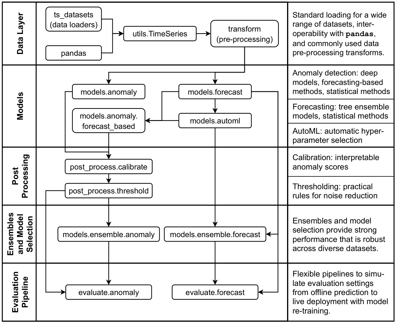
Figure 1: Architecture of modules in Merlion.
图 1: Merlion 中的模块架构。
2.2 Models
2.2 模型
Since no single model can perform well across all time series and all use cases, it is important to provide users the flexibility to choose from a broad suite of he t erogenous models. Merlion implements many diverse models for both forecasting and anomaly detection. These include statistical methods, tree-based models, and deep learning approaches, among others. To transparently expose all these options to an end user, we unify all Merlion models under two common API’s, one for forecasting, and one for anomaly detection. All models are initialized with a config object that contains implementation-specific hyper parameters, and support a model.train(time series) method.
由于没有任何单一模型能够在所有时间序列和所有用例中表现良好,因此为用户提供从广泛的异构模型中选择的灵活性非常重要。Merlion 实现了许多用于预测和异常检测的多样化模型,包括统计方法、基于树的模型和深度学习方法等。为了透明地向最终用户展示所有这些选项,我们将所有 Merlion 模型统一在两个通用 API 下,一个用于预测,另一个用于异常检测。所有模型都通过包含实现特定超参数的配置对象进行初始化,并支持 model.train(time series) 方法。
Given a general multivariate time series $T=(U^{(1)},\dots,U^{(d)})$ , forecasters are trained to predict the values of a single target univariate $U^{(k)}$ . One can then obtain a model’s forecast of $U^{(k)}$ for a set of future time stamps by calling model.forecast(time stamps).
给定一个通用的多元时间序列 $T=(U^{(1)},\dots,U^{(d)})$,预测模型被训练来预测单个目标单变量 $U^{(k)}$ 的值。然后,可以通过调用 model.forecast(time stamps) 来获得模型对 $U^{(k)}$ 在未来时间戳上的预测值。
Analogously, one can obtain an anomaly detector’s sequence of anomaly scores for the time series $T$ by simply calling model.get anomaly score(time series). The handling of univariate vs. multivariate time series is implementation-specific (e.g. some algorithms look for an anomaly in any of the uni variate s, while others may look for anomalies in specific uni variate s). Notably, forecasters can also be used for anomaly detection by treating the residual between the true and predicted value of a target univariate $U^{(k)}$ as an anomaly score. These forecast-based anomaly detectors support both model.forecast(time stamps) and model.get anomaly score(time series).
类似地,可以通过调用 model.get_anomaly_score(time_series) 获取时间序列 $T$ 的异常检测器异常分数序列。单变量与多变量时间序列的处理方式因实现而异(例如,某些算法会在任意单变量中寻找异常,而另一些算法可能会在特定单变量中寻找异常)。值得注意的是,预测器也可以用于异常检测,方法是将目标单变量 $U^{(k)}$ 的真实值与预测值之间的残差视为异常分数。这些基于预测的异常检测器同时支持 model.forecast(time_stamps) 和 model.get_anomaly_score(time_series)。
For models that require additional computation, we implement a Layer interface that is the basis for the autoML features we offer. Layer is used to implement additional logic on top of existing model definitions that would not be properly fitted into the model code itself. Examples include seasonality detection and hyper parameter tuning (see §3.2 for more details). The Layer is an interface that implements three methods: generate theta for generating hyper parameter candidates $\theta$ , evaluate theta for evaluating the quality of $\theta$ ’s, and set_theta for applying the chosen $\theta$ to the underlying model. A separate class Forecaster Auto ML Base implements forecast and train methods that leverage methods from the Layer class to complete the forecasting model.
对于需要额外计算的模型,我们实现了一个 Layer 接口,这是我们提供的 autoML (自动机器学习) 功能的基础。Layer 用于在现有模型定义之上实现额外的逻辑,这些逻辑无法直接融入模型代码本身。例如,季节性检测和超参数调优(详见 §3.2)。Layer 是一个接口,它实现了三个方法:generate_theta 用于生成超参数候选 $\theta$,evaluate_theta 用于评估 $\theta$ 的质量,set_theta 用于将选定的 $\theta$ 应用到基础模型中。一个单独的类 Forecaster Auto ML Base 实现了 forecast 和 train 方法,这些方法利用 Layer 类的方法来完成预测模型。
Finally, all models support the ability to condition their predictions on historical data time series prev that is distinct from the data used for training. One can obtain these conditional predictions by calling model.forecast(time stamps, time series prev) or model.get anomaly score(time series, time series prev).
最后,所有模型都支持基于历史数据时间序列 prev 进行预测的能力,这些历史数据与用于训练的数据不同。可以通过调用 model.forecast(time stamps, time series prev) 或 model.get anomaly score(time series, time series prev) 来获取这些条件预测。
2.3 Post-Processing
2.3 后处理
All anomaly detectors have a post_rule which applies important post-processing to the output of model.get anomaly score(time series). This includes calibration (§4.2.1), which ensures that anomaly scores correspond to standard deviation units and are therefore interpret able and consistent between different models, and threshold ing (§4.2.2) rules to reduce the number of false positives. One can directly obtain post-processed anomaly scores by calling model.get anomaly label(time series).
所有异常检测器都有一个后处理规则 (post_rule),它对 model.get anomaly score(time series) 的输出进行重要的后处理。这包括校准 (calibration) (§4.2.1),确保异常分数对应于标准偏差单位,因此在不同模型之间具有可解释性和一致性,以及阈值处理 (thresholding) 规则 (§4.2.2) 以减少误报数量。通过调用 model.get anomaly label(time series) 可以直接获得后处理后的异常分数。
2.4 Ensembles and Model Selection
2.4 集成与模型选择
Ensembles are structured as a model that represents a combination of multiple underlying models. For this purpose we have a base Ensemble Base class that abstracts the process of obtaining predictions $Y_{1},\dots,Y_{m}$ from $m$ underlying models on a single time series $T$ , and a Combiner class that then combines results $Y_{1},\dots,Y_{m}$ into the output of the ensemble. These combinations include traditional mean ensembles, as well as model selection based on evaluation metrics like sMAPE. Concrete implementations implement the forecast or get anomaly score methods on top of the tools provided by Ensemble Base, and their train method automatically handles dividing the data into train and validation splits if needed (e.g. for model selection).
集成模型是由多个基础模型组合而成的结构。为此,我们有一个基础的 Ensemble Base 类,它抽象了从单个时间序列 $T$ 上的 $m$ 个基础模型获取预测 $Y_{1},\dots,Y_{m}$ 的过程,以及一个 Combiner 类,它将结果 $Y_{1},\dots,Y_{m}$ 组合成集成模型的输出。这些组合包括传统的均值集成,以及基于评估指标(如 sMAPE)的模型选择。具体实现在 Ensemble Base 提供的工具之上实现了 forecast 或 get anomaly score 方法,并且它们的 train 方法在需要时自动处理将数据划分为训练集和验证集(例如用于模型选择)。
2.5 Evaluation Pipeline
2.5 评估流程
When a time series model is deployed live in production, training and inference are usually not performed in batch on a full time series. Rather, the model is re-trained at a regular cadence, and where possible, inference is performed in a streaming mode. To more realistically simulate this setting, we provide a Eva lu at or Base class which implements the following evaluation loop:
当时间序列模型在生产环境中部署时,通常不会对整个时间序列进行批量训练和推理。相反,模型会定期重新训练,并且在可能的情况下,推理会以流模式进行。为了更真实地模拟这种场景,我们提供了一个 Eva lu at or Base 类,它实现了以下评估循环:
We also provide a wide range of evaluation metrics for both forecasting and anomaly detection, implemented as the enums Forecast Metric and TSADMetric, respectively. Finally, we provide scripts benchmark forecast.py and benchmark anomaly.py which allow users to use this logic to easily evaluate model performance on any dataset included in the ts datasets module. We report experimental results using these scripts in §5.
我们还为预测和异常检测提供了多种评估指标,分别实现为枚举类型 Forecast Metric 和 TSADMetric。最后,我们提供了脚本 benchmark forecast.py 和 benchmark anomaly.py,使用户能够利用此逻辑轻松评估模型在 ts datasets 模块中包含的任何数据集上的性能。我们在第 5 节中使用这些脚本报告了实验结果。
3 Time Series Forecasting
3 时间序列预测
In this section, we introduce Merlion’s specific univariate and multivariate forecasting models, provide algorithmic details on Merlion’s autoML and ensembling modules for forecasting, and describe the metrics used for experimental evaluation in §5.1 and §5.2.
在本节中,我们介绍了Merlion的特定单变量和多变量预测模型,提供了Merlion的自动机器学习(autoML)和预测集成模块的算法细节,并描述了在第5.1节和第5.2节中用于实验评估的指标。
3.1 Models
3.1 模型
Merlion contains a number of models for univariate time series forecasting. These include classic statistcal methods like ARIMA (Auto Regressive Integrated Moving Average), SARIMA (Seasonal ARIMA) and ETS (Error, Trend, Seasonality), more recent algorithms like Prophet (Taylor and Letham, 2017), our previous production algorithm MSES (Cassius et al., 2021), and a deep auto regressive LSTM (Hochreiter and Schmid huber, 1997), among others.
Merlion包含多种用于单变量时间序列预测的模型。这些模型包括经典的统计方法,如ARIMA(自回归积分滑动平均)、SARIMA(季节性ARIMA)和ETS(误差、趋势、季节性),以及最近提出的算法,如Prophet(Taylor和Letham,2017),我们之前的生产算法MSES(Cassius等,2021),以及深度自回归LSTM(Hochreiter和Schmidhuber,1997)等。
The multivariate forecasting models we use are based on auto regression and tree ensemble algorithms. For the auto regression algorithm, we adopt the Vector Auto regression model (VAR, Lütkepohl (2005)) that captures the relationship between multiple sequences as they change over time. For tree ensembles, we consider Random Forest (RF, Ho (1995)) and Gradient Boosting (GB, Ke et al. (2017)) as the base models. However, without appropriate modifications, tree ensemble models can be unsuitable for the general practice of time series forecasting. First, their output is a fixed-length vector, so it is not straightforward to obtain their forecasts for arbitrary prediction horizons. Second, these multivariate forecasting models often have incompatible data workflows or APIs that make it difficult to directly apply them for univariate prediction.
我们使用的多元预测模型基于自回归和树集成算法。对于自回归算法,我们采用了向量自回归模型 (VAR, Lütkepohl (2005)),该模型捕捉了多个序列随时间变化的关系。对于树集成模型,我们将随机森林 (RF, Ho (1995)) 和梯度提升 (GB, Ke et al. (2017)) 作为基础模型。然而,如果没有适当的修改,树集成模型可能不适合时间序列预测的常规实践。首先,它们的输出是固定长度的向量,因此要获得任意预测范围的预测并不直接。其次,这些多元预测模型通常具有不兼容的数据工作流程或 API,这使得直接将其应用于单变量预测变得困难。
To overcome these obstacles, we propose an auto regressive forecasting strategy for our tree ensemble models, RF Forecaster and GB Forecaster. For a $d$ -variable time series, these models forecast the value of all $d$ variables in the time series for time $t_{k}$ , and they condition on this prediction to auto regressive ly forecast for time $t_{k+1}$ . We thus enable these models to produce a forecast for an arbitrary prediction horizon, similar to more traditional models like VAR. Additionally, all our multivariate forecasting models share common APIs with the univariate forecasting models, and are therefore universal for both the univariate and the multivariate forecasting tasks. A full list of supported models can be found in the API documentation.
为了克服这些障碍,我们为树集成模型 RF Forecaster 和 GB Forecaster 提出了一种自回归预测策略。对于一个 $d$ 变量的时间序列,这些模型预测时间 $t_{k}$ 的所有 $d$ 个变量的值,并基于此预测自回归地预测时间 $t_{k+1}$ 的值。因此,我们使这些模型能够像 VAR 等更传统的模型一样,为任意预测范围生成预测。此外,我们所有的多变量预测模型与单变量预测模型共享相同的 API,因此对单变量和多变量预测任务都是通用的。支持的完整模型列表可以在 API 文档中找到。
3.2 AutoML and Model Selection
3.2 AutoML 与模型选择
The AutoML module for time series forecasting models is slightly different from autoML for covent ional machine learning models, as we consider not only conventional hyperparameter optimization, but also the detection of some characteristics of time series. Take the SARIMA $(p,d,q)\times(P,Q,D)_{m}$ model as an example. Its hyper parameters include the auto regressive parameter $p$ , difference order $d$ , moving average parameter $q$ , seasonal autoregressive parameter $P$ , seasonal difference order $D$ , seasonal moving average parameter $Q$ , and seasonality $m$ . While we use SARIMA as a motivating example, note that automatic seasonality detection can directly enhance other models like ETS and Prophet (Taylor and Letham, 2017). Meanwhile, choosing the appropriate (seasonal) difference order can yield a representation of the time series that makes the prediction task easier for any model.
时间序列预测模型的 AutoML 模块与常规机器学习模型的 AutoML 略有不同,因为我们不仅考虑常规的超参数优化,还考虑时间序列的某些特征的检测。以 SARIMA $(p,d,q)\times(P,Q,D)_{m}$ 模型为例,其超参数包括自回归参数 $p$、差分阶数 $d$、移动平均参数 $q$、季节性自回归参数 $P$、季节性差分阶数 $D$、季节性移动平均参数 $Q$ 以及季节性 $m$。虽然我们以 SARIMA 为例,但需要注意的是,自动季节性检测可以直接增强其他模型,如 ETS 和 Prophet (Taylor 和 Letham, 2017)。同时,选择合适的(季节性)差分阶数可以生成时间序列的表示,使预测任务对任何模型都更加容易。
Typically, we first analyze the time series to choose the seasonality $m$ . Following the idea from the theta method (As si mako poul os and Niko lo poul os, 2000), we say that a time series has seasonality $m$ at significance level $a$ if
通常,我们首先分析时间序列以选择季节性 $m$# 2023年医院三基考试每日一练《药师(这是一个关于获取当前时间并输出为指定格式的Python代码示例。以下是一个简单的实现:
import datetime
def get_current_time():
# 获取当前时间
now = datetime.datetime.now()
# 格式化为字符串,例如:2023#!# ball mill grinding and beneficiation process
# **Introduction to React.js**
## **1. What is React.js?**
# dg
A simple command line interface for querying the Dark Globe API.
# 1. 环境搭建
## 1.1 开发环境
- 开发板:飞凌iMX.6ULL开发板
- 开发环境:Ub#Use these commands to delete all of the files and<issue_start><issue_comment# autorun
description of autorun

where \$r_{k}\$ is the lag \$k\$ auto correlation, \$m\$ is the number of periods within a seasonal cycle, \$n\$ is the sample size, and \$\Phi^{-1}\$ is the quantile function of the standard normal distribution. By default, we set the significance at \$a=0.05\$ to reflect the \$95\%\$ prediction intervals.
其中 \$r_{k}\$ 是滞后 \$k\$ 的自相关,\$m\$ 是一个季节性周期内的期数,\$n\$ 是样本大小,且 \$\Phi^{-1}\$ 是标准正态分布的分位数函数。默认情况下,我们将显著性设为 \$a=0.05\$,以反映 \$95\%\$ 的预测区间。
Next, we select the seasonal difference order \$\boldsymbol{D}\$ by estimating the strength of the seasonal component with the time series decomposition method (Cleveland et al., 1990). Suppose the time series can be written as \$y=T+S+R\$ , where \$T\$ is the smoothed trend component, \$S\$ is the seasonal component and \$R\$ is the remainder. Then, the strength of the seasonality (Wang et al., 2006) is
接下来,我们通过时间序列分解方法 (Cleveland et al., 1990) 估计季节性成分的强度,从而选择季节性差分阶数 \$\boldsymbol{D}\$。假设时间序列可以表示为 \$y=T+S+R\$,其中 \$T\$ 是平滑的趋势成分,\$S\$ 是季节性成分,\$R\$ 是残差。那么,季节性强度 (Wang et al., 2006) 为

Note that a time series with strong seasonality will have \$F_{S}\$ close to 1 since \$\mathrm{Var}(R)\$ is much smaller than \$\operatorname{Var}(S+R)\$ . If \$F_{S}\$ is large, we adopt the seasonal difference operation. Thus, we choose \$D\$ by success vi ely decomposing the time series and differ enc ing it based on the detected seasonality until \$F_{S}\$ is relatively small. We can then choose the difference order \$d\$ by applying successive KPSS unit-root tests to the seasonally differenced data.
需要注意的是,具有强季节性的时间序列的 \$F_{S}\$ 会接近 1,因为 \$\mathrm{Var}(R)\$ 远小于 \$\operatorname{Var}(S+R)\$。如果 \$F_{S}\$ 较大,我们采用季节性差分操作。因此,我们通过逐步分解时间序列并根据检测到的季节性进行差分来选择 \$D\$,直到 \$F_{S}\$ 相对较小。然后,我们可以通过对季节性差分数据应用连续的 KPSS 单位根检验来选择差分阶数 \$d\$。
Once \$m\$ , \$D\$ , and \$d\$ are selected, we can choose the remaining hyper parameters \$p\$ , \$q\$ , \$P\$ , and \$Q\$ by minimizing the AIC (Akaike Information Criterion) via grid search. Because the parameter space is exponentially large if we ex hast iv ely enumerate all the hyper parameter combinations, we follow the step-wise search method of Hyndman and Khandakar (2008).
一旦选择了 \$m\$、\$D\$ 和 \$d\$,我们可以通过网格搜索最小化 AIC(赤池信息准则)来选择剩余的超参数 \$p\$、\$q\$、\$P\$ 和 \$Q\$。由于参数空间在穷举所有超参数组合时呈指数级增长,因此我们遵循 Hyndman 和 Khandakar (2008) 提出的逐步搜索方法。
Bhatnagar et al.
Bhatnagar 等人
To further speed up the training time of the autoML module, we propose the following approximation strategy: we obtain an initial list of candidate models that achieve good performance after relatively few optimization iterations; we then re-train each of these candidates until model convergence, and finally select the best model by AIC.
为了进一步加快 autoML 模块的训练时间,我们提出了以下近似策略:首先获得一个在相对较少的优化迭代后表现良好的候选模型初始列表;然后重新训练这些候选模型直到模型收敛,最后通过 AIC 选择最佳模型。
# 3.3 Ensembles
3.3 集成方法
Ensembles of forecasters in Merlion allow a user to transparently combine models in two ways. First, we support traditional ensembles that report the mean or median value predicted by all the models at each timestamp. Second, we support automated model selection. When performing model selection, we divide the training data into train and validation splits, train each model on the training split, and obtain its predictions for the validation split. We then evaluate the quality of those predictions using a user-specified evaluation metric like sMAPE or RMSE (§3.4), and return the model that achieved the best performance after re-training it on the full training data. These features are useful in many practical scenarios, as they can greatly reduce the amount of human intervention needed when deploying a model.
Merlion中的预测器集成允许用户以两种方式透明地组合模型。首先,我们支持传统集成,报告每个时间戳所有模型预测的平均值或中位数。其次,我们支持自动化模型选择。在执行模型选择时,我们将训练数据分为训练集和验证集,在训练集上训练每个模型,并获取其在验证集上的预测。然后,我们使用用户指定的评估指标(如sMAPE或RMSE)评估这些预测的质量,并在完整训练数据上重新训练后返回表现最佳的模型。这些功能在许多实际场景中非常有用,因为它们可以大大减少部署模型时所需的人工干预。
# 3.4 Evaluation Metrics
# 3.4 评估指标
There are many ways to evaluate the accuracy of a forecasting model. Given a time series with \$n\$ observations, let \$y_{t}\$ denote the observed value at time \$t\$ and \$\hat{y}_{t}\$ denote the corresponding predicted value. Then the forecasting error \$e_{t}\$ at time \$t\$ is \$y_{t}-\hat{y}_{t}\$ . Error measures based on absolute or squared errors are widely used, and they are formuated as
评估预测模型准确性的方法有很多。给定一个包含 \$n\$ 个观测值的时间序列,设 \$y_{t}\$ 表示时间 \$t\$ 的观测值,\$\hat{y}_{t}\$ 表示相应的预测值。那么时间 \$t\$ 的预测误差 \$e_{t}\$ 为 \$y_{t}-\hat{y}_{t}\$。基于绝对误差或平方误差的误差度量方法被广泛使用,其公式为

respectively. Unfortunately, these measures cannot be compared across time series that are on different scales. To achive scale-independence, one alternative approach is to use percentage errors based on the observed values. One typical measure is sMAPE (Makridakis and Hibon, 2000), defined as:
分别。遗憾的是,这些指标无法在不同尺度的时间序列之间进行比较。为了实现尺度独立性,一种替代方法是使用基于观测值的百分比误差。一个典型的指标是 sMAPE (Makridakis and Hibon, 2000),其定义为:
\$\$
\mathrm{sMAPE}=\frac{1}{n}\sum_{t=1}^{n}\frac{\left\lvert e_{t}\right\rvert}{\left\lvert y_{t}\right\rvert+\left\lvert\hat{y}_{t}\right\rvert}*200(\%),
\$\$
\$\$
\mathrm{sMAPE}=\frac{1}{n}\sum_{t=1}^{n}\frac{\left\lvert e_{t}\right\rvert}{\left\lvert y_{t}\right\rvert+\left\lvert\hat{y}_{t}\right\rvert}*200(\%),
\$\$
Unfortunately, sMAPE has the disadvantage of being ill-defined if \$y_{t}\$ and \$\hat{y}_{t}\$ are both close to zero. To address this issue, one alternative measure is MARRE, which is defined as
遗憾的是,如果 \$y_{t}\$ 和 \$\hat{y}_{t}\$ 都接近零,sMAPE 的缺陷在于其定义不明确。为解决这一问题,一个替代的衡量指标是 MARRE,其定义为

However, MARRE is not always suitable for non-stationary time series, where the scale of the data may evolve over time. Merlion’s Forecast Metric enum supports all the above classes of evaluation metrics, as well as others detailed in the API documentation. By default, we evaluate forecasting results by sMAPE, but users may manually specify alternatives if their application calls for it.
然而,MARRE 并不总是适用于非平稳时间序列,因为数据规模可能# ---
<issue_start><issue_comment># Data Science
Data Science codes
# 4 Time Series Anomaly Detection
# 4 时间序列异常检测<|end▁of▁sentence|>
In this section, we introduce Merlion’s specific univariate and multivariate anomaly detection models, provide algorithmic details on Merlion’s post-processing and ensembling modules for anomaly detection, and describe the metrics used for experimental evaluation in §5.3 and §5.4.
在本节中,我们介绍了 Merlion 的特定单变量和多变量异常检测模型,提供了 Merlion 后处理和集成模块的算法细节,并描述了在 §5.3 和 §5.4 中用于实验评估的指标。<|end▁of▁sentence|>
# 4.1 Models
4.1 模型
Merlion contains a number of models that are specialized for univariate time series anomaly detection. These fall into two groups: forecasting-based and statistical. Because forecasters in Merlion predict the value of a specific univariate in a general time series, they are straightforward to adapt for anomaly detection. The anomaly score is simply the residual between the predicted and true time series value, optionally normalized by the underlying forecaster’s predicted standard error (if it produces one).
Merlion 包含一系列专门用于单变量时间序列异常检测的模型。这些模型分为两大类:基于预测的和统计的。由于 Merlion 中的预测器能够预测一般时间序列中特定单变量的值,因此它们很容易适应异常检测。异常分数简单地就是预测值与真实时间序列值之间的残差,可以选择性地通过底层预测器的预测标准误差进行归一化(如果它提供了标准误差)。
For univariate statistical methods, we support Spectral Residual (Ren et al., 2019), as well as two simple baselines WindStats and ZMS. WindStats divides each week into windows (e.g. 6 hours), and computes the anomaly score \$s_{t}=(x_{t}-\mu(t))/\sigma(t)\$ , where \$\mu(t)\$ and \$\sigma(t)\$ are the historical mean and standard deviation of the window in question (e.g. 12pm to 6pm on Monday). ZMS computes k-lags ∆t(k) \$\Delta_{t}^{(k)}=x_{t}-x_{t-k}\$ for \$k=1,2,4,8,\dots\$ , and computes the anomaly score \$s_{t}=\operatorname*{max}_{k}({\Delta}_{t}^{(k)}-\mu^{(k)})/\sigma^{(k)}\$ , where \$\mu^{(k)}\$ and \$\sigma^{(k)}\$ are the mean and standard deviation of each \$k\$ -lag.
对于单变量统计方法,我们支持谱残差(Spectral Residual)方法(Ren 等人,2019),以及两种简单的基线方法 WindStats 和 ZMS。WindStats 将每周划分为多个窗口(例如 6 小时),并计算异常分数 \$s_{t}=(x_{t}-\mu(t))/\sigma(t)\$,其中 \$\mu(t)\$ 和 \$\sigma(t)\$ 分别是该窗口(例如周一 12 点到 6 点)的历史均值和标准差。ZMS 计算 k 阶滞后 \$\Delta_{t}^{(k)}=x_{t}-x_{t-k}\$,其中 \$k=1,2,4,8,\dots\$,并计算异常分数 \$s_{t}=\operatorname*{max}_{k}({\Delta}_{t}^{(k)}-\mu^{(k)})/\sigma^{(k)}\$,其中 \$\mu^{(k)}\$ 和 \$\sigma^{(k)}\$ 分别是每个 \$k\$ 滞后的均值和标准差。<|end▁of▁sentence|>
In addition to models that are specialized for univariate anomaly detection, we support both statistical methods and deep learning models that can handle both univariate and multivariate anomaly detection. The statistical methods include Isolation Forest (Liu et al., 2008) and Random Cut Forest Guha et al. (2016), while the deep learning models include an auto encoder (Baldi, 2012), a Deep Auto encoding Gaussian Mixture Model (DAGMM, Zong et al. (2018)), a LSTM encoder-decoder (Sutskever et al., 2014), and a variation al auto encoder (Kingma and Welling, 2013). A full list can be found in the API documentation.
除了专门用于单变量异常检测的模型外,我们还支持统计方法和深度学习模型,这些方法可以处理单变量和多变量异常检测。统计方法包括孤立森林 (Isolation Forest, Liu et al., 2008) 和随机切割森林 (Random Cut Forest, Guha et al., 2016),而深度学习模型包括自编码器 (auto encoder, Baldi, 2012)、深度自编码高斯混合模型 (Deep Auto encoding Gaussian Mixture Model, DAGMM, Zong et al., 2018)、LSTM编码器-解码器 (LSTM encoder-decoder, Sutskever et al., 2014) 和变分自编码器 (variational auto encoder, Kingma and Welling, 2013)。完整的列表可以在API文档中找到。
# 4.2 Post-Processing
# 4.2 后处理<|end▁of▁sentence|>
Merlion supports two key post-processing steps for anomaly detectors: calibration and threshold ing. Calibration is important for improving model in te pre t ability, while threshold ing converts a sequence of continuous anomaly scores into discrete labels and reduces the false positive rate.
Merlion支持异常检测器的两个关键后处理步骤:校准(calibration)和阈值处理(thresholding)。校准对于提高模型的可解释性非常重要,而阈值处理将连续的异常分数序列转换为离散标签,并降低误报率。
# 4.2.1 Calibration
4.2.1 校准
All anomaly detectors in Merlion return anomaly scores \$s_{t}\$ such that \$|s_{t}|\$ is positively correlated with the severity of the anomaly. However, the scales and distributions of these anomaly scores vary widely. For example, Isolation Forest (Liu et al., 2008) returns an anomaly score \$s_{t}\in[0,1]\$ where \$-\log_{2}(1-s_{t})\$ is a node’s depth in a binary tree; Spectral Residual (Ren et al., 2019) returns an un normalized saliency map; DAGMM (Zong et al., 2018) returns a negative log probability.
Merlion 中的所有异常检测器都返回异常分数 \$s_{t}\$,使得 \$|s_{t}|\$ 与异常的严重程度呈正相关。然而,这些异常分数的尺度和分布差异很大。例如,Isolation Forest (Liu et al., 2008) 返回一个异常分数 \$s_{t}\in[0,1]\$,其中 \$-\log_{2}(1-s_{t})\$ 是二叉树中节点的深度;Spectral Residual (Ren et al., 2019) 返回一个未归一化的显著图;DAGMM (Zong et al., 2018) 返回一个负对数概率。
To successfully use a model, one must be able to interpret the anomaly scores it returns. However, this prevents many models from being immediately useful to users who are unfamiliar with their specifc implementations. Calibration bridges this gap by making all anomaly scores interpret able as z-scores, i.e. values drawn from a standard normal distribution.
要成功使用模型,必须能够解释其返回的异常分数。然而,这阻碍了许多模型对不熟悉其具体实现的用户的即时可用性。通过将所有异常分数校准为z分数(即来自标准正态分布的值),校准解决了这一差距。
Let \$\Phi:\mathbb{R}\rightarrow[0,1]\$ be the cumulative distribution function (CDF) of the standard normal distribution. A calibrator \$C:\mathbb{R}\rightarrow\mathbb{R}\$ converts a raw anomaly score \$s_{t}\$ into a calibrated score \$z_{t}\$ such that \$\mathbb{P}[|z_{t}|>\alpha]=\Phi(\alpha)-\Phi(-\alpha)=2\Phi(\alpha)-1\$ , i.e. \$|z_{t}|\$ follows the same distribution as the absolute value of a standard normal random variable. If \$F_{s}:\mathbb{R}\rightarrow[0,1]\$ is the CDF of the absolute raw anomaly scores \$|s_{t}|\$ , we can compute the re calibrated score as
设 \$\Phi:\mathbb{R}\rightarrow[0,1]\$ 为标准正态分布的累积分布函数 (CDF)。校准器 \$C:\mathbb{R}\rightarrow\mathbb{R}\$ 将原始异常分数 \$s_{t}\$ 转换为校准分数 \$z_{t}\$,使得 \$\mathbb{P}[|z_{t}|>\alpha]=\Phi(\alpha)-\Phi(-\alpha)=2\Phi(\alpha)-1\$,即 \$|z_{t}|\$ 遵循与标准正态随机变量的绝对值相同的分布。如果 \$F_{s}:\mathbb{R}\rightarrow[0,1]\$ 是原始异常分数 \$|s_{t}|\$ 的 CDF,我们可以计算重新校准的分数为

Notably, this is also the optimal transport map between the two distributions, i.e. the mapping which transfers mass from one distribution to the other in a way that minimizes the \$\ell_{1}\$ transportation cost (Villani, 2003).
值得注意的是,这也是两个分布之间的最优传输映射,即以最小化\$\ell_{1}\$传输成本的方式将一个分布的质量转移到另一个分布的映射 (Villani, 2003)。
In practice, we estimate the calibration function \$C\$ using the empirical CDF \$\hat{F}_{s}\$ and a monotone spline interpol at or (Fritsch and Butland, 1984) for intermediate values. This simple post-processing step dramatically increases the in te pre t ability of the anomaly scores returned by individual models. It also enables us to create ensembles of diverse anomaly detectors as discussed in §4.3. This functionality is enabled by default for all anomaly detection models.
在实践中,我们使用经验 CDF \$\hat{F}_{s}\$ 和单调样条插值器(Fritsch and Butland, 1984)来估计校准函数 \$C\$ 的中间值。这一简单的后处理步骤显著提高了单个模型返回的异常分数的可解释性。它还使我们能够创建多样化的异常检测器集成,如 §4.3 中所述。此功能默认在所有异常检测模型中启用。
# 4.2.2 Threshold ing
# 4.2.2 阈值处理
The most common way to decide whether an individual timestamp \$t\$ as anomalous, is to compare the anomaly score \$s_{t}\$ against a threshold \$\tau\$ . However, in many real-world systems, a human is alerted every time an anomaly is detected. A high false positive rate will lead to fatigue from the end users who have to investigate each alert, and may result in a system whose users think it is unreliable.
判断单个时间戳 \$t\$ 是否为异常的最常见方法是将异常分数 \$s_{t}\$ 与阈值 \$\tau\$ 进行比较。然而,在许多实际系统中,每次检测到异常时都会向人类发出警报。高误报率会导致终端用户因不得不调查每个警报而感到疲劳,并可能导致用户认为系统不可靠。
A common way to circumvent this problem is including additional automated checks that must pass before a human is alerted. For instance, our system may only fire an alert if there are two timestamps \$t_{1},t_{2}\$ within a short window (e.g. 1 hour) with a high anomaly score, i.e. \$|s_{t_{1}}|>\tau\$ and \$|s_{t_{2}}|>\tau\$ . Moreover, if we know that anomalies typically last 2 hours, our system can simply suppress all alerts occurring within 2 hours of a recent one, as those alerts likely correspond to the same underlying incident. Often, one or both of these steps can greatly increase precision without adversely impacting recall. As such, they are commonplace in production systems.
解决此问题的常见方法是包含额外的自动化检查,这些检查必须在警报触发之前通过。例如,我们的系统可能仅在短时间窗口内(例如1小时)有两个时间戳\$t_{1},t_{2}\$且具有高异常分数时才会触发警报,即\$|s_{t_{1}}|>\tau\$和\$|s_{t_{2}}|>\tau\$。此外,如果我们知道异常通常持续2小时,系统可以简单地抑制在最近警报发生2小时内的所有警报,因为这些警报可能对应于相同的基础事件。通常,这些步骤中的一个或两个可以显著提高精确度,而不会对召回率产生不利影响。因此,它们在生产系统中很常见。
Merlion implements all these features in the user-configurable Aggregate Alarms postprocessing rule, and by default, it is enabled for all anomaly detection models.
Merlion 在用户可配置的 Aggregate Alarms 后处理规则中实现了所有这些功能,默认情况下,所有异常检测模型都启用了该规则。
# 4.3 Ensembles
4.3 集成方法
Because both time series and the anomalies they contain are incredibly diverse, it is unlikely that a single model will be the best for all use cases. In principle, a he t erogenous ensemble of models may generalize better than any individual model in that ensemble. Unfortunately, as mentioned in §4.2.1, constructing an ensemble is not straightforward due to the vast differences in anomaly scores returned by various models.
由于时间序列及其包含的异常情况极为多样,单一模型不太可能适用于所有用例。原则上,异构模型集成可能比集成中的任何单个模型具有更好的泛化能力。然而,正如第4.2.1节所述,由于不同模型返回的异常分数存在巨大差异,构建集成并非易事。
However, because we can rely on the anomaly scores of all Merlion models to be interpretable as z-scores, we can construct an ensemble of anomaly detectors by simply reporting the mean calibrated anomaly score returned by each individual model, and then applying a threshold (a la §4.2.2) on this combined anomaly score. Empirically, we find that ensembles robustly achieve the strongest or competitive performance (relative to the baselines considered) across multiple open source and internal datasets for both univariate (Table 10) and multivariate (Table 13) anomaly detection.
然而,由于我们可以依赖所有 Merlion 模型的异常分数作为可解释的 z 分数,因此我们可以通过简单地报告每个模型返回的平均校准异常分数来构建异常检测器的集成,然后在此组合异常分数上应用阈值(如 §4.2.2)。经验表明,集成方法在多个开源和内部数据集上,无论是单变量(表 10)还是多变量(表 13)异常检测,均能稳健地达到最强或具有竞争力的性能(相对于所考虑的基线)。
# 4.4 Evaluation Metrics
4.4 评估指标
The key challenge in designing an appropriate evaluation metric for time series anomaly detection lies in the fact that anomalies are almost always windows of time, rather than discrete points. Thus, while it is easy to compute the pointwise (PW) precision, recall, and F1 score of a predicted anomaly label sequence relative to the ground truth label sequence, these metrics do not reflect a quantity that human operators care about.
设计合适的时间序列异常检测评估指标的关键挑战在于,异常通常是时间窗口而非离散点。因此,虽然计算预测的异常标签序列相对于真实标签序列的点对点(PW)精度、召回率和F1分数很容易,但这些指标并不能反映出人类操作者关心的实际数量。<|end▁of▁sentence|>
Xu et al. (2018) propose point-adjusted (PA) metrics as a solution to this problem: if any point in a ground truth anomaly window is labeled as anomalous, all points in the segment are treated as true positives. If no anomalies are flagged in the window, all points are labeled as false negatives. Any predicted anomalies outside of anomalous windows are treated as false positives. Precision, recall, and F1 can be computed based on these adjusted true/false positive/negative counts. However, the disadvantage of PA metrics is that they are biased to reward models for detecting long anomalies more than short ones.
Xu et al. (2018) 提出了点调整 (PA) 指标作为此问题的解决方案:如果地面实况异常窗口中的任何一点被标记为异常,则整个段中的所有点都被视为真正例。如果窗口中没有标记异常,则所有点都被标记为假反例。任何在异常窗口之外预测的异常都被视为假正例。基于这些调整后的真正例/假正例/假反例计数,可以计算精确率、召回率和F1值。然而,PA指标的缺点是它们偏向于奖励检测长时间异常的模型,而不是短时间异常。
Hundman et al. (2018) propose revised point-adjusted (RPA) metrics as a closely related alternative: if any point in a ground truth anomaly window is labeled as anomalous, one true positive is registered. If no anomalies are flagged in the window, one false negative is recorded. Any predicted anomalies outside of anomalous windows are treated as false positives. These metrics address the shortcomings of PA metrics, but they do penalize false positives more heavily than alternatives.
Hundman 等人 (2018) 提出了修订点调整 (RPA) 指标作为一种密切相关的替代方案:如果地面实况异常窗口中的任何点被标记为异常,则记录一个真正例。如果窗口中未标记任何异常,则记录一个假反例。任何在异常窗口之外的预测异常都被视为假正例。这些指标解决了 PA 指标的缺点,但它们对假正例的惩罚比其他替代方案更重。
Merlion’s TSADMetric enum supports all 3 classes of evaluation metrics (PW, PA, and RPA), as well as the mean time to detect an anomaly. By default, we evaluate RPA metrics, but users may manually specify alternatives if their application calls for it.
Merlion 的 TSADMetric 枚举支持所有 3 类评估指标(PW、PA 和 RPA),以及检测异常的平均时间。默认情况下,我们评估 RPA 指标,但如果应用需要,用户可以手动指定其他指标。
# 5 Experiments
# 5 实验
In the experiments section, we show benchmark results generated by using Merlion with popular baseline models across several time series datasets. The purpose of this section is not to obtain state-of-the-art results. Rather, most algorithms listed are strong baselines. To avoid the possible risk of label leaking through manual hyper parameter tuning, for all experiments, we evaluate all models with a single choice of sensible default hyper parameters and data pre-processing, regardless of dataset.
在实验部分,我们展示了使用 Merlion 与多个时间序列数据集上的流行基线模型生成的基准测试结果。本节的目的是为了获得最先进的结果,而是为了展示大多数列出的算法作为强基线的表现。为了避免通过手动超参数调整可能导致标签泄露的风险,对于所有实验,我们使用单一合理的默认超参数和数据预处理来评估所有模型,无论数据集如何。
Table 2: Summary of M4 dataset for univariate forecasting.
<html><body><table><tr><td>M4</td><td>Hourly</td><td>Daily</td><td>Weekly</td><td>Monthly</td><td>Quarterly</td><td>Yearly</td></tr><tr><td># Time Series RealData? Availability</td><td>414 Public</td><td>4,227 Public</td><td>359 Public</td><td>48,000 Public</td><td>24,000 Public</td><td>23,000 Public</td></tr><tr><td>Prediction Horizon</td><td>6</td><td>8</td><td>18</td><td>13</td><td>14</td><td>48</td></tr></table></body></html>
表 2: 单变量预测的 M4 数据集摘要。
| M4 | 每小时 | 每日 | 每周 | 每月 | 每季度 | 每年 |
| --- | --- | --- | --- | --- | --- | --- |
| # 时间序列 真实数据? 可用性 | 414 公开 | 4,227 公开 | 359 公开 | 48,000 公开 | 24,000 公开 | 23,000 公开 |
| 预测范围 | 6 | 8 | 18 | 13 | 14 | 48 |
Table 3: Summary of internal datasets for univariate forecasting.
<html><body><table><tr><td></td><td>Int_UF1</td><td>Int_UF2</td><td>Int_UF3</td></tr><tr><td># Time Series</td><td>21</td><td>6</td><td>4</td></tr><tr><td>Real Data?</td><td></td><td></td><td></td></tr><tr><td>Availability</td><td>Internal</td><td>Internal</td><td>Internal</td></tr><tr><td>Train Split</td><td>First 75%</td><td>First 25%</td><td>First 25%</td></tr></table></body></html>
表 3: 单变量预测内部数据集总结。
| | Int_UF1 | Int_UF2 | Int_UF3 |
| --- | --- | --- | --- |
| # 时间序列 | 21 | 6 | 4 |
| 真实数据? | | | |
| 可用性 | 内部 | 内部 | 内部 |
| 训练集划分 | 前 75% | 前 25% | 前 25% |
# 5.1 Univariate Forecasting
5.1 单变量预测
# 5.1.1 Datasets and Evaluation
# 5.1.1 数据集与评估
We primarily evaluate our models on the M4 benchmark (Makridakis et al., 2018, 2020), an influential time series forecasting competition. The dataset contains 100, 000 time series from diverse domains including financial, industry, and demographic forecasting. It has sampling frequencies ranging from hourly to yearly. Table 2 summarizes the dataset. We additionally evaluate on three internal datasets of cloud KPIs, which we describe in Table 3. For all datasets, models are trained and evaluated in the offline batch prediction setting, with a pre-defined prediction horizon equal to the size of the test split. To mitigate the effect of outliers, we report both the mean and median sMAPE for each method.
我们主要在 M4 基准(Makridakis 等人,2018,2020)上评估我们的模型,这是一个具有影响力的时间序列预测竞赛。该数据集包含来自金融、工业和人口统计预测等多个领域的 100,000 个时间序列,采样频率从每小时到每年不等。表 2 总结了该数据集。我们还在三个内部云 KPI 数据集上进行了评估,如表 3 所示。对于所有数据集,模型在离线批量预测设置中进行训练和评估,预测范围与测试集大小相同。为了减轻异常值的影响,我们报告了每种方法的平均值和中位数 sMAPE。<|end▁of▁sentence|>
# 5.1.2 Models
5.1.2 模型
We compare ARIMA (Auto Regressive Integrated Moving Average), Prophet (Taylor and Letham, 2017), ETS (Error, Trend, Seasonality), and MSES (the previous production solution, Cassius et al. (2021)). For ARIMA, Prophet and ETS, we also consider our autoML variants that perform automatic seasonality detection and hyper parameter tuning, as described in §3.2. These are implemented using the merlion.models.automl module.
我们比较了 ARIMA (Auto Regressive Integrated Moving Average)、Prophet (Taylor 和 Letham, 2017)、ETS (Error, Trend, Seasonality) 以及 MSES (前生产解决方案,Cassius 等人 (2021))。对于 ARIMA、Prophet 和 ETS,我们还考虑了自动季节检测和超参数调优的 autoML 变体,如 §3.2 所述。这些变体使用 merlion.models.automl 模块实现。
# 5.1.3 Results
# 5.1.3 结果<|end▁of▁sentence|>
Table 4 and 5 respectively show the performance of each model on the public and internal datasets. Table 6 shows the average improvement achieved by using the autoML module. For ARIMA, we find a clear improvement by using the AutoML module for all datasets. While the improvement is statistically significant for Prophet and AutoETS overall, the actual change is small on most datasets except M4 \$-\$ Hourly and Int \$-\$ UF2. This is because many of the other datasets don’t contain well-defined seasonal i ties; additionally, Prophet already has
表 4 和表 5 分别展示了各个模型在公开数据集和内部数据集上的表现。表 6 展示了使用 autoML 模块后取得的平均改进。对于 ARIMA 模型,我们发现使用 AutoML 模块后,所有数据集都有显著的改进。虽然 Prophet 和 AutoETS 模型在整体上也有统计显著的改进,但在大多数数据集上实际变化较小,除了 M4 \$-\$ Hourly 和 Int \$-\$ UF2 数据集。这是因为许多其他数据集并没有明确的季节性特征;此外,Prophet 已经具备了一定的季节性处理能力。
<html><body><table><tr><td></td><td>M4</td><td>Hourly</td><td>M4</td><td>Daily</td><td>M4</td><td>Weekly</td></tr><tr><td>sMAPE</td><td>Mean</td><td>Median</td><td>Mean</td><td>Median</td><td>Mean</td><td>Median</td></tr><tr><td>MSES ARIMA Prophet ETS</td><td>32.45 33.54 18.08</td><td>16.89 19.27 6.92</td><td>5.87 3.23 11.67</td><td>3.97 2.06 5.99</td><td>16.53 9.29 19.98</td><td>9.96 5.38 11.26</td></tr><tr><td>AutoSARIMA AutoProphet AutoETS</td><td>13.61 16.49 19.23</td><td>4.73 6.20 5.33</td><td>3.29 11.67 3.07</td><td>2.00 5.98 1.98</td><td>8.30 20.01 9.32</td><td>5.09 11.63</td></tr><tr><td></td><td>M4</td><td>Monthly</td><td>M4</td><td>Quarterly</td><td>M4</td><td>5.15 Yearly</td></tr><tr><td>sMAPE MSES</td><td>Mean 25.40</td><td>Median 13.69</td><td>Mean 19.03</td><td>Median 9.53</td><td>Mean 21.63</td><td>Median 12.11</td></tr><tr><td>ARIMA Prophet ETS</td><td>17.66 20.64 14.32</td><td>10.41 11.00</td><td>13.37 24.53</td><td>8.27 12.81</td><td>16.37 30.23</td><td>10.34 19.24</td></tr></table></body></html>
| | M4 | Hourly | M4 | Daily | M4 | Weekly |
|---------|------|--------|------|------|------|--------|
| sMAPE | Mean | Median | Mean | Median | Mean | Median |
| MSES ARIMA Prophet ETS | 32.45 33.54 18.08 | 16.89 19.27 6.92 | 5.87 3.23 11.67 | 3.97 2.06 5.99 | 16.53 9.29 19.98 | 9.96 5.38 11.26 |
| AutoSARIMA AutoProphet AutoETS | 13.61 16.49 19.23 | 4.73 6.20 5.33 | 3.29 11.67 3.07 | 2.00 5.98 1.98 | 8.30 20.01 9.32 | 5.09 11.63 |
| | M4 | Monthly | M4 | Quarterly | M4 | 5.15 Yearly |
| sMAPE MSES | Mean 25.40 | Median 13.69 | Mean 19.03 | Median 9.53 | Mean 21.63 | Median 12.11 |
| ARIMA Prophet ETS | 17.66 20.64 14.32 | 10.41 11.00 | 13.37 24.53 | 8.27 12.81 | 16.37 30.23 | 10.34 19.24 |<|end▁of▁sentence|>
<html><body><table><tr><td colspan="3">Int</td><td colspan="2">Int UF2</td><td colspan="2">Int UF3</td></tr><tr><td>sMAPE</td><td>Mean</td><td>Median</td><td>Mean</td><td>Median</td><td>Mean</td><td>Median</td></tr><tr><td>MSES ARIMA Prophet</td><td>33.50 24.00</td><td>32.60 19.42</td><td>32.30 25.89 30.93</td><td>14.45 24.40 38.54</td><td>3.882 5.94 72.55</td><td>3.771 6.15 78.27</td></tr><tr><td>ETS AutoSARIMA AutoProphet AutoETS</td><td>17.02 15.98 56.43</td><td>16.36 15.10 41.99</td><td>25.10 17.45 26.35</td><td>24.19 9.98 24.19</td><td>3.55 3.42 69.32</td><td>3.32 3.41 78.37</td></tr></table></body></html>
| Int | Int UF2 | Int UF3 |
| sMAPE | Mean | Median | Mean | Median | Mean | Median |
| MSES ARIMA Prophet | 33.50 24.00 | 32.60 19.42 | 32.30 25.89 30.93 | 14.45 24.40 38.54 | 3.882 5.94 72.55 | 3.771 6.15 78.27 |
| ETS AutoSARIMA AutoProphet AutoETS | 17.02 15.98 56.43 | 16.36 15.10 41.99 | 25.10 17.45 26.35 | 24.19 9.98 24.19 | 3.55 3.42 69.32 | 3.32 3.41 78.37 |
Table 5: Mean and Median sMAPE achived by univariate forecasting models on internal datasets. All models were evaluated without retraining. Best results are in bold.
表 5: 单变量预测模型在内部数据集上实现的平均和中位 sMAPE。所有模型均未重新训练的情况下进行评估。最佳结果以粗体显示。
<html><body><table><tr><td>ARIMA → AutoSARIMA Prophet → AutoProphet ETS → AutoETS</td><td>5.03 3 (p = 0.010) 1.01 1 (p=0 0.035) 2.96 (p = 0 0.039)</td></tr></table></body></html>
ARIMA → AutoSARIMA Prophet → AutoProphet ETS → AutoETS
5.03 3 (p = 0.010) 1.01 1 (p = 0.035) 2.96 (p = 0.039)
Table 6: Average reduction (improvment) in sMAPE achieved by applying autoML. \$p\$ -value is from a 2-sided paired sample \$t\$ -test. Our autoML module improves all 3 models at significance level \$p=0.05\$ .
表 6: 应用 autoML 后 sMAPE 的平均减少(改进)情况。\$p\$ 值来自双样本配对 \$t\$ 检验。我们的 autoML 模块在显著水平 \$p=0.05\$ 下改进了所有 3 个模型。<|end▁of▁sentence|>
Table 7: Summary of multivariate forecasting datasets.
<html><body><table><tr><td></td><td>Power Grid</td><td>Seattle Trail</td><td>Solar Plant</td><td>Int MF</td></tr><tr><td># Time Series</td><td>1</td><td>1</td><td>1</td><td>21</td></tr><tr><td># Variables</td><td>10</td><td>5</td><td>405</td><td>22</td></tr><tr><td>Real Data?</td><td></td><td></td><td></td><td></td></tr><tr><td>Availability</td><td>Public</td><td>Public</td><td>Public</td><td>Internal</td></tr><tr><td>Data Source</td><td>Energy Demand</td><td>Trail Traffic</td><td>Power Generation</td><td>Cloud KPIs</td></tr><tr><td>Train Split</td><td>First 70%</td><td>First 70%</td><td>First 70%</td><td>First 75%</td></tr><tr><td>Granularity</td><td>1h</td><td>x</td><td>30min</td><td>10s</td></tr><tr><td>Reference</td><td>ene (2018)</td><td>sea (2018)</td><td>Shih et al. 1. (2019)</td><td></td></tr></table></body></html>
表 7: 多变量预测数据集总结。
| | Power Grid | Seattle Trail | Solar Plant | Int MF |
|----------|------------|---------------|-------------|--------|
| # 时间序列 | 1 | 1 | 1 | 21 |
| # 变量 | 10 | 5 | 405 | 22 |
| 真实数据? | | | | |
| 可用性 | 公开 | 公开 | 公开 | 内部 |
| 数据来源 | 能源需求 | 步道流量 | 发电量 | 云 KPI |
| 训练分割 | 前 70% | 前 70% | 前 70% | 前 75% |
| 粒度 | 1h | x | 30min | 10s |
| 参考文献 | ene (2018) | sea (2018) | Shih et al. 1. (2019) | |
some pre-defined seasonality detection (daily, weekly, and yearly), but these datasets contain time series with hourly seasonal i ties.
一些预定义的季节性检测(每日、每周和每年),但这些数据集包含具有每小时季节性的时间序列。
While there is no clear winner across all datasets, AutoSarima and AutoETS consistently outperform other methods. The overall performance of AutoSarima is slightly better than AutoETS, but AutoSarima is much slower to train. Therefore, we believe that AutoETS is a good “default” model for new users or early exploration.
虽然没有在所有数据集中明显的赢家,但 AutoSarima 和 AutoETS 始终优于其他方法。AutoSarima 的整体表现略优于 AutoETS,但 AutoSarima 的训练速度要慢得多。因此,我们认为 AutoETS 是新用户或早期探索的良好“默认”模型。
# 5.2 Multivariate Forecasting
5.2 多元预测
# 5.2.1 Datasets and Evaluation
# 5.2.1 数据集与评估
We collect public and internal datasets (Table 7) and train models on a training split of the data. For some datasets, we resample the data with given granular i ties. For each time series, we train the models on the training split to predict the first univariate as a target sequence. While we don’t re-train the model, we use the evaluation pipeline described in §2.5 to increment ally obtain predictions for the test split using a rolling window. We predict time series values for the next 3 timestamps, while conditioning the prediction on the previous 21 timestamps. We obtain these 3-step predictions at every timestamp in the test split, and evaluate the quality of the prediction using sMAPE where possible, and RMSE otherwise.
我们收集了公开和内部的数据集(表 7),并在数据的训练集上进行模型训练。对于某些数据集,我们以给定的粒度对数据进行重采样。对于每个时间序列,我们在训练集上训练模型,以预测第一个单变量作为目标序列。虽然我们没有重新训练模型,但我们使用第 2.5 节中描述的评估管道,通过滚动窗口逐步获得测试集的预测。我们预测接下来 3 个时间戳的时间序列值,同时以之前的 21 个时间戳为条件进行预测。我们在测试集的每个时间戳上获得这些 3 步预测,并尽可能使用 sMAPE 评估预测质量,否则使用 RMSE。
# 5.2.2 Models
5.2.2 模型
The multivariate forecasting models we use are based on the auto regression and tree ensemble algorithms. We compare VAR (Lütkepohl, 2005), GB Forecaster based on the Gradient Boosting algorithm (Ke et al., 2017) and RF Forecaster based on the Random Forest algorithm (Ho, 1995). We discuss the implementation details of these models in §3.1. For the GB Forecster and RF Forecaster, we use our proposed auto regression strategy to enable them to forecast for an arbitrary prediction horizon.
我们使用的多元预测模型基于自回归和树集成算法。我们比较了VAR (Lütkepohl, 2005)、基于梯度提升算法 (Gradient Boosting) 的GB Forecaster (Ke et al., 2017) 和基于随机森林算法 (Random Forest) 的RF Forecaster (Ho, 1995)。我们将在§3.1中讨论这些模型的实现细节。对于GB Forecaster和RF Forecaster,我们使用我们提出的自回归策略,使它们能够预测任意预测范围。
# 5.2.3 Results
5.2.3 结果
Table 8 reports the performance of each model. We find that our proposed auto gres sion-based tree ensemble model GB Forecaster achieves the best results on three of the four datasets and is competitive with the best result on the fourth. While the VAR model shows competitive
表 8 报告了每个模型的性能。我们发现,我们提出的基于自回归的树集成模型 GB Forecaster 在四个数据集中的三个上取得了最佳结果,并且在第四个数据集上与最佳结果具有竞争力。而 VAR 模型显示出竞争力
<html><body><table><tr><td></td><td>Power Grid</td><td>Seattle Trail</td><td>Solar Plant</td><td colspan="2">Int _MF</td></tr><tr><td></td><td>sMAPE (1 TS)</td><td>RMSE (1 TS)</td><td>RMSE (1 TS)</td><td>sMAPE (mean)</td><td>sMAPE (median)</td></tr><tr><td>VAR</td><td>1.131</td><td>968048</td><td>10.30</td><td>22.11</td><td>17.87</td></tr><tr><td>GBForecaster</td><td>1.705</td><td>41.66</td><td>3.712</td><td>14.05</td><td>12.18</td></tr><tr><td>RF Forecaster</td><td>3.256</td><td>44.20</td><td>4.633</td><td>23.25</td><td>19.82</td></tr></table></body></html>
| | 电网 | 西雅步道 | 太阳能电厂 | Int _MF |
|:---|:---|:---|:---|:---|:---|
| | sMAPE (1 TS) | RMSE (1 TS) | RMSE (1 TS) | sMAPE (均值) | sMAPE (中值) |
| VAR | 1.131 | 968048 | 10.30 | 22.11 | 17.87 |
| GBForecaster | 1.705 | 41.66 | 3.712 | 14.05 | 12.18 |
| RF Forecaster | 3.256 | 44.20 | 4.633 | 23.25 | 19.82 |
Table 8: Performance of multivariate forecasting models. All models were evaluated without retraining. Best results are in bold. We report RMSE instead of sMAPE for the Seattle Trail and Solar Plant datasets because a large portion of the data values ( \$13\%\$ and \$55\%\$ respectively) are equal to 0, making them unsuitable for sMAPE. 1 TS means that there is only one time series in the dataset.
表 8: 多元预测模型的性能。所有模型均未重新训练进行评估。最佳结果以粗体显示。对于 Seattle Trail 和 Solar Plant 数据集,我们报告 RMSE 而不是 sMAPE,因为大部分数据值(分别为 \$13\%\$ 和 \$55\%\$)等于 0,这使得它们不适合使用 sMAPE。1 TS 表示数据集中只有一个时间序列。
Table 9: Summary of univariate anomaly detection datasets.
<html><body><table><tr><td></td><td>Int_UA</td><td>NAB</td><td>AIOps</td><td>UCR</td></tr><tr><td># Time Series Real data?</td><td>26 √</td><td>58 47/58 real</td><td>29</td><td>250 Mixed</td></tr><tr><td>Availability Data Source</td><td>Internal Cloud KPIs</td><td>Public Various</td><td>Public Cloud KPIs</td><td>Public Various</td></tr><tr><td>Train split</td><td>First 25%</td><td>First 15%</td><td>First 50%</td><td>First 30%</td></tr><tr><td>Supervised?</td><td>No</td><td>No</td><td>Train labels</td><td>Test labels</td></tr><tr><td>Threshold</td><td></td><td></td><td></td><td></td></tr><tr><td></td><td>4.0</td><td>3.5</td><td></td><td></td></tr><tr><td></td><td></td><td></td><td></td><td></td></tr><tr><td>Reference</td><td></td><td>Lavin and Ahmad (2015)</td><td>aio (2018)</td><td>Dau et al. (2018)</td></tr></table></body></html>
表 9: 单变量异常检测数据集总结。
| | Int_UA | NAB | AIOps | UCR |
| --- | --- | --- | --- | --- |
| # 时间序列 真实数据? | 26 √ | 58 47/58 真实 | 29 | 250 混合 |
| 可用性 数据源 | 内部云 KPIs | 公开 多种 | 公开云 KPIs | 公开 多种 |
| 训练分割 | 前 25% | 前 15% | 前 50% | 前 30% |
| 有监督? | 否 | 否 | 训练标签 | 测试标签 |
| 阈值 | | | | |
| | 4.0 | 3.5 | | |
| | | | | |
| 参考文献 | | Lavin 和 Ahmad (2015) | aio (2018) | Dau 等 (2018) |
performance on some datasets, it is not as robust. For example, the Seattle Trail dataset has large outliers (several orders of magnitude larger than the mean) that dramatically impact the performance of VAR. For this reason, we believe that GB Forecaster is a good “default” model for new users or early exploration.
在某些数据集上性能表现不佳,且不够稳健。例如,Seattle Trail 数据集中存在较大的异常值(比均值大几个数量级),这显著影响了 VAR 的性能。因此,我们认为 GB Forecaster 是新用户或早期探索时的良好“默认”模型。
# 5.3 Univariate Anomaly Detection
# 5.3 单变量异常检测
# 5.3.1 Datasets and Evaluation
5.3.1 数据集与评估
We report results on four public and internal datasets (Table 9). For the internal dataset and the Numenta Anomaly Benchmark (NAB, Lavin and Ahmad (2015)), we choose a single (calibrated) detection threshold for all time series and all algorithms. For the AIOps challenge (aio, 2018), we use the labeled anomalies in the training split of each time series to choose the detection threshold that optimizes F1 on the training split; for the UC Riverside Time Series Anomaly Archive (Dau et al., 2018), we choose the detection threshold that optimizes F1 on the test split. This is because the dataset is incredibly diverse (so a single threshold doesn’t apply to all time series), and there are no anomalies present in the training split. Table 9 summarizes these datasets and evaluation choices.
我们在四个公共和内部数据集上报告了结果(表 9)。对于内部数据集和 Numenta 异常基准(NAB, Lavin and Ahmad (2015)),我们为所有时间序列和所有算法选择一个(校准的)检测阈值。对于 AIOps 挑战赛(aio, 2018),我们使用每个时间序列训练集中的标记异常来选择在训练集上优化 F1 的检测阈值;对于 UC Riverside 时间序列异常档案(Dau et al., 2018),我们选择在测试集上优化 F1 的检测阈值。这是因为数据集非常多样化(因此单个阈值不适用于所有时间序列),并且在训练集中没有异常。表 9 总结了这些数据集和评估选择。<|end▁of▁sentence|>
We use the evaluation pipeline described in §2.5 to evaluate each model. After training an initial model on the training split of a time series, we re-train the model unsupervised
我们使用在第2.5节中描述的评估流程来评估每个模型。在时间序列的训练集上训练初始模型后,我们以无监督的方式重新训练模型
<html><body><table><tr><td></td><td>Int UA</td><td>NAB</td><td>AIOps</td><td>UCR</td><td>△ F1 (vs. best)</td></tr><tr><td>ARIMA</td><td>0.531</td><td>0.395</td><td>0.227</td><td>0.313</td><td>0.148 ± 0.099</td></tr><tr><td>AutoETS</td><td>0.296</td><td>0.350</td><td>0.097</td><td>0.334</td><td>0.245 ± 0.042</td></tr><tr><td>AutoProphet</td><td>0.343</td><td>0.323</td><td>0.310</td><td>0.418</td><td>0.166 ± 0.062</td></tr><tr><td>Isolation Forest</td><td>0.436</td><td>0.244</td><td>0.347</td><td>0.461</td><td>0.142 ± 0.111</td></tr><tr><td>Random Cut Forest</td><td>0.248</td><td>0.337</td><td>0.314</td><td>0.568</td><td>0.148 ± 0.132</td></tr><tr><td>Spectral Residual</td><td>0.340</td><td>0.153</td><td>0.338</td><td>0.469</td><td>0.189 ± 0.150</td></tr><tr><td>WindStats s(baseline)</td><td>0.225</td><td>0.247</td><td>0.324</td><td>0.306</td><td>0.239 ± 0.114</td></tr><tr><td>ZMS (baseline)</td><td>0.486</td><td>0.290</td><td>0.340</td><td>0.427</td><td>0.129 ± 0.094</td></tr><tr><td>Ensemble (ours)</td><td>0.500</td><td>0.548</td><td>0.396</td><td>0.476</td><td>0.034±0.044</td></tr></table></body></html>
| | Int UA | NAB | AIOps | UCR | △ F1 (vs. best) |
| --- | --- | --- | --- | --- | --- |
| ARIMA | 0.531 | 0.395 | 0.227 | 0.313 | 0.148 ± 0.099 |
| AutoETS | 0.296 | 0.350 | 0.097 | 0.334 | 0.245 ± 0.042 |
| AutoProphet | 0.343 | 0.323 | 0.310 | 0.418 | 0.166 ± 0.062 |
| Isolation Forest | 0.436 | 0.244 | 0.347 | 0.461 | 0.142 ± 0.111 |
| Random Cut Forest | 0.248 | 0.337 | 0.314 | 0.568 | 0.148 ± 0.132 |
| Spectral Residual | 0.340 | 0.153 | 0.338 | 0.469 | 0.189 ± 0.150 |
| WindStats s(baseline) | 0.225 | 0.247 | 0.324 | 0.306 | 0.239 ± 0.114 |
| ZMS (baseline) | 0.486 | 0.290 | 0.340 | 0.427 | 0.129 ± 0.094 |
| Ensemble (ours) | 0.500 | 0.548 | 0.396 | 0.476 | 0.034±0.044 |
Table 10: F1 scores achieved by univariate anomaly detection models. All models were evaluated using batch prediction, daily re-training, and hourly re-training; we report the best F1 achieved by any of the re-training schedules. We also report the average gap (over datasets) in F1 between each model and the best model. Best results are in bold.
表 10: 单变量异常检测模型实现的 F1 分数。所有模型均使用批量预测、每日重新训练和每小时重新训练进行评估;我们报告了任何重新训练计划实现的最佳 F1。我们还报告了每个模型与最佳模型之间 F1 的平均差距(跨数据集)。最佳结果以粗体显示。
either daily or hourly on the full data until that point (without adjusting the calibrator or threshold). We then increment ally obtain predicted anomaly scores for the full time series, in a way that simulates a live deployment scenario. We also consider batch prediction, where the initial trained model predicts anomaly scores for the entire test split in a single step, without any re-training. Note that the UCR dataset does not contain timestamps; we treat it as if it is sampled once per minute, but this is an imperfect assumption. We consider only batch prediction and “daily” retraining for this dataset for efficiency reasons.
在完整数据上每天或每小时进行一次预测(不调整校准器或阈值)。然后,我们逐步获得整个时间序列的预测异常分数,以模拟实时部署场景。我们还考虑批量预测,即初始训练模型在单一步骤中预测整个测试集的异常分数,无需重新训练。需要注意的是,UCR 数据集不包含时间戳;我们假设它每分钟采样一次,但这是一个不完美的假设。出于效率考虑,我们仅对该数据集进行批量预测和“每日”重新训练。
# 5.3.2 Models
5.3.2 模型
We evaluate two classes of models: forecast-based anomaly detectors and statistical methods. For forecast-based methods, we use ARIMA, AutoETS, and Auto Prophet (as described in §5.1). For statistical methods, we use Isolation Forest (Liu et al., 2008), Random Cut Forest (Guha et al., 2016), and Spectral Residual (Ren et al., 2019), as well as two simple baselines WindStats and ZMS (§4.1). We also consider an ensemble of AutoETS, RRCF, and ZMS (using the algorithm described in §4.3).
我们评估了两类模型:基于预测的异常检测器和统计方法。对于基于预测的方法,我们使用了 ARIMA、AutoETS 和 Auto Prophet(如第 5.1 节所述)。对于统计方法,我们使用了 Isolation Forest (Liu et al., 2008)、Random Cut Forest (Guha et al., 2016) 和 Spectral Residual (Ren et al., 2019),以及两个简单的基线方法 WindStats 和 ZMS(第 4.1 节)。我们还考虑了 AutoETS、RRCF 和 ZMS 的集成(使用第 4.3 节描述的算法)。
# 5.3.3 Results
5.3.3 结果
Table 10 reports the revised point-adjusted F1 score achieved by each model on each dataset. We report the best F1 score achieved by any of the 3 re-training schedules (for efficiency reasons, we only consider batch prediction and daily re-training for Auto Prophet). We find that our proposed ensemble of AutoETS, RRCF, and ZMS achieves the best performance on two of the four datasets, and the second-best on the others; overall, it has the smallest average gap in F1 score relative to the best model for each dataset (along with the smallest variance in this gap). For this reason, we believe that it is a good “default” model for new users or early exploration.
表 10 报告了每个模型在每个数据集上经过调整的 F1 分数。我们报告了三种重新训练计划中任何一种所达到的最佳 F1 分数(出于效率原因,我们仅考虑 Auto Prophet 的批量预测和每日重新训练)。我们发现,我们提出的 AutoETS、RRCF 和 ZMS 集成在四个数据集中的两个上表现最佳,在其他数据集上表现次佳;总体而言,相对于每个数据集的最佳模型,它的 F1 分数差距最小(且差距的方差也最小)。因此,我们认为它是新用户或早期探索的一个很好的“默认”模型。
Table 11 examines the impact of the re-training schedule for each model, averaged across all datasets. We find that daily and hourly re-training of forecasting-based models and our proposed ensemble can greatly improve their anomaly detection performance. However, in practice, the ideal re-training frequency may require some experimentation to choose. Interestingly, the impact of frequent re-training is unclear for most statistical models.
表 11 检验了每种模型的重新训练计划对整体性能的影响(在所有数据集上取平均值)。我们发现,对于基于预测的模型和我们提出的集成方法,每天或每小时重新训练可以显著提高其异常检测性能。然而,在实践中,理想的重新训练频率可能需要通过实验来确定。有趣的是,对于大多数统计模型来说,频繁重新训练的影响尚不明确。<|end▁of▁sentence|>
Merlion: A Machine Learning Library for Time Series
<html><body><table><tr><td></td><td>Daily</td><td>Hourly</td></tr><tr><td>ARIMA</td><td>0.162 (p =0.001)</td><td>0.227 (p<0.001)</td></tr><tr><td>AutoETS</td><td>0.088 (p =0.017)</td><td>0.058 (p = 0.325)</td></tr><tr><td>AutoProphet</td><td>0.028 (p =0.013)</td><td></td></tr><tr><td>Isolation Forest</td><td>0.006 (p = 0.779)</td><td>0.019 (p = 0.567)</td></tr><tr><td>Random Cut Forest</td><td>0.024 (p = 0.396)</td><td>0.033 (p = 0.337)</td></tr><tr><td>Spectral Residual</td><td>-0.090 (p = 0.075)</td><td>-0.109 (p = 0.004)</td></tr><tr><td>WindStats (baseline)</td><td>0.044 (p =0.098)</td><td>0.017 (p = 0.145)</td></tr><tr><td>ZMS (baseline)</td><td>0.005 (p = 0.929)</td><td>0.011 (p =0.872)</td></tr><tr><td>Ensemble (ours)</td><td>0.147 (p = 0.023)</td><td>0.183 (p = 0.009)</td></tr></table></body></html>
Merlion: 一个用于时间序列的机器学习库
| | 每日 | 每小时 |
|----------|------|--------|
| ARIMA | 0.162 (p =0.001) | 0.227 (p<0.001) |
| AutoETS | 0.088 (p =0.017) | 0.058 (p = 0.325) |
| AutoProphet | 0.028 (p =0.013) | |
| Isolation Forest | 0.006 (p = 0.779) | 0.019 (p = 0.567) |
| Random Cut Forest | 0.024 (p = 0.396) | 0.033 (p = 0.337) |
| Spectral Residual | -0.090 (p = 0.075) | -0.109 (p = 0.004) |
| WindStats (baseline) | 0.044 (p =0.098) | 0.017 (p = 0.145) |
| ZMS (baseline) | 0.005 (p = 0.929) | 0.011 (p =0.872) |
| Ensemble (ours) | 0.147 (p = 0.023) | 0.183 (p = 0.009) |
Table 11: Average change in F1 (relative to no re-training) achieved by re-training models both daily and hourly. \$p\$ -value is from a 2-sided paired sample \$t\$ -test. Re-training makes a significant improvement for the forecasting models (first block) and the ensemble. However, the statistical models (second block) benefit only marginally (if at all). Table 12: Summary of multivariate anomaly detection datasets.
<html><body><table><tr><td></td><td>SMD</td><td>SMAP</td><td>MSL</td><td>Int _MA</td></tr><tr><td># Time Series</td><td>28</td><td>1</td><td>1</td><td>20</td></tr><tr><td># Variables</td><td>38</td><td>25</td><td>55</td><td>5</td></tr><tr><td>Real data?</td><td><</td><td></td><td><</td><td></td></tr><tr><td>Availability</td><td>Public</td><td>Public</td><td>Public</td><td>Internal</td></tr><tr><td>Data Source</td><td>Cloud KPIs</td><td>SatelliteData</td><td>Mars Rover</td><td>Cloud KPIs</td></tr><tr><td>Train split</td><td>First 50%</td><td>First 25%</td><td>First 45%</td><td>First 50%</td></tr><tr><td>Supervised?</td><td>No</td><td>No</td><td>No</td><td>No</td></tr><tr><td>Threshold</td><td>3.0</td><td>3.5</td><td>3.0</td><td>3.5</td></tr><tr><td>Reference</td><td>Su et al. (2019)</td><td>Hundman et al. (2018)</td><td>Hundman et al. (2018)</td><td></td></tr></table></body></html>
表 11: 每日和每小时重新训练模型相对于不重新训练的 F1 平均变化。\$p\$ 值来自双侧配对样本 \$t\$ 检验。重新训练对预测模型(第一块)和集成模型有显著改进。然而,统计模型(第二块)的改进微乎其微(如果有的话)。表 12: 多元异常检测数据集摘要。
| | SMD | SMAP | MSL | Int_MA |
|----------|-----|------|-----|--------|
| # 时间序列 | 28 | 1 | 1 | 20 |
| # 变量 | 38 | 25 | 55 | 5 |
| 真实数据? | < | | < | |
| 可用性 | 公开 | 公开 | 公开 | 内部 |
| 数据来源 | 云 KPI | 卫星数据 | 火星探测器 | 云 KPI |
| 训练分割 | 前 50% | 前 25% | 前 45% | 前 50% |
| 有监督? | 否 | 否 | 否 | 否 |
| 阈值 | 3.0 | 3.5 | 3.0 | 3.5 |
| 参考文献 | Su et al. (2019) | Hundman et al. (2018) | Hundman et al. (2018) | |
# 5.4 Multivariate Anomaly Detection
# 5# c++ - /* reference: https://justicehui.github.io/ps/2019/06#include <iostream>
#include <#include <#include <#include <++.+#include <iostream>
#include <++.h>#include#include<iostream>
#include <bits/stdc++.h>
#include<bits/stdc++.h>
#include <++.h, 1, 10, 11/*
*#include <int main ( ) { if ( a + ( b ) ) { int a ; a = b ; } while ( c ) { } }
# 5.4.1 Datasets and Evaluation
5.4.1 数据集与评估
The evaluation setting for multivariate anomaly detection is nearly identical to that for univariate anomaly detection. Table 12 describes the multivariate time series anomaly detection datasets in this epxeriment. Note that we treat anomaly detection on all these datasets as a fully unsupervised learning task. The main difference from the univariate setting is that we consider only batch predictions and weekly retraining (rather than batch predictions, daily re-training, and hourly retraining) for efficiency reasons.
多元异常检测的评估设置与单变量异常检测几乎相同。表 12 描述了本实验中使用的多元时间序列异常检测数据集。需要注意的是,我们将这些数据集上的异常检测视为完全无监督学习任务。与单变量设置的主要区别在于,出于效率考虑,我们仅考虑批量预测和每周重新训练(而不是批量预测、每日重新训练和每小时重新训练)。<|end▁of▁sentence|>
<html><body><table><tr><td></td><td>SMD</td><td>SMAP</td><td>MSL</td><td>Int tMA</td><td>△ F1 (vs. best)</td></tr><tr><td>Isolation Forest</td><td>0.388</td><td>0.211</td><td>0.226</td><td>0.252</td><td>0.129±0.025</td></tr><tr><td>Random Cut Forest</td><td>0.500</td><td>0.108</td><td>0.312</td><td>0.313</td><td>0.091 ± 0.110</td></tr><tr><td>Autoencoder</td><td>0.264</td><td>0.357</td><td>0.355</td><td>0.357</td><td>0.065 ± 0.114</td></tr><tr><td>DAGMM</td><td>0.191</td><td>0.037</td><td>0.135</td><td>0.182</td><td>0.262 ± 0.067</td></tr><tr><td>LSTM Encoder-Decoder</td><td>0.344</td><td>0.357</td><td>0.381</td><td>0.301</td><td>0.053 ± 0.074</td></tr><tr><td>Variational Autoencoder</td><td>0.318</td><td>0.187</td><td>0.381</td><td>0.322</td><td>0.097 ± 0.093</td></tr><tr><td>Ensemble (ours)</td><td>0.403</td><td>0.291</td><td>0.357</td><td>0.341</td><td>0.051±0.038</td></tr></table></body></html>
| | SMD | SMAP | MSL | Int tMA | △ F1 (vs. best) |
|------------------------|-------|-------|-------|---------|------------------|
| Isolation Forest | 0.388 | 0.211 | 0.226 | 0.252 | 0.129±0.025 |
| Random Cut Forest | 0.500 | 0.108 | 0.312 | 0.313 | 0.091 ± 0.110 |
| Autoencoder | 0.264 | 0.357 | 0.355 | 0.357 | 0.065 ± 0.114 |
| DAGMM | 0.191 | 0.037 | 0.135 | 0.182 | 0.262 ± 0.067 |
| LSTM Encoder-Decoder | 0.344 | 0.357 | 0.381 | 0.301 | 0.053 ± 0.074 |
| Variational Autoencoder| 0.318 | 0.187 | 0.381 | 0.322 | 0.097 ± 0.093 |
| Ensemble (ours) | 0.403 | 0.291 | 0.357 | 0.341 | 0.051±0.038 |
Table 13: F1 scores achieved by multivariate anomaly detection models. All models were evaluated using batch prediction and weekly re-training; we report the best F1 achieved by any of the re-training schedules. We also report the average gap (over datasets) in F1 between each model and the best model. Best results are in bold.
表 13: 多元异常检测模型达到的 F1 分数。所有模型均使用批量预测和每周重新训练进行评估;我们报告了任何重新训练计划中实现的最佳 F1。我们还报告了每个模型与最佳模型之间 F1 的平均差距(跨数据集)。最佳结果以粗体显示。<|end▁of▁sentence|>
<html><body><table><tr><td></td><td>Weekly</td></tr><tr><td>Isolation Forest Random Cut Forest</td><td>0.006 (p =0.796) 0.036 p =0.130</td></tr><tr><td>Autoencoder DAGMM</td><td>-0.075 (p=0.352) 0.057 (p=0.032</td></tr><tr><td>LSTMEncoder-Decoder VariationalAutoencoder</td><td>0.001 p = 0.970) 0.020 =