A Multi-Task Semantic Decomposition Framework with Task-specific Pre-training for Few-Shot NER
基于任务特定预训练的少样本命名实体识别多任务语义分解框架
ABSTRACT
摘要
The objective of few-shot named entity recognition is to identify named entities with limited labeled instances. Previous works have primarily focused on optimizing the traditional token-wise classification framework, while neglecting the exploration of information based on NER data characteristics. To address this issue, we propose a Multi-Task Semantic Decomposition Framework via Joint Task-specific Pre-training (MSDP) for few-shot NER. Drawing inspiration from demonstration-based and contrastive learning, we introduce two novel pre-training tasks: Demonstration-based Masked Language Modeling (MLM) and Class Contrastive Discrimination. These tasks effectively incorporate entity boundary information and enhance entity representation in Pre-trained Language Models (PLMs). In the downstream main task, we introduce a multitask joint optimization framework with the semantic decomposing method, which facilitates the model to integrate two different semantic information for entity classification. Experimental results of two few-shot NER benchmarks demonstrate that MSDP consistently outperforms strong baselines by a large margin. Extensive analyses validate the effectiveness and generalization of MSDP.
少样本命名实体识别的目标是在有限标注实例下识别命名实体。先前研究主要聚焦于优化传统的基于token的分类框架,而忽视了基于NER数据特性的信息探索。为解决这一问题,我们提出通过联合任务特定预训练的多任务语义分解框架(MSDP)。受基于演示和对比学习的启发,我们引入两项新颖的预训练任务:基于演示的掩码语言建模(MLM)和类别对比判别。这些任务有效整合了实体边界信息,并增强了预训练语言模型(PLM)中的实体表示能力。在下游主任务中,我们采用语义分解方法构建多任务联合优化框架,促使模型融合两种不同语义信息进行实体分类。两个少样本NER基准测试的实验结果表明,MSDP始终以显著优势超越强基线模型。大量分析验证了MSDP的有效性和泛化能力。
CCS CONCEPTS
CCS概念
• Computing methodologies $\rightarrow$ Artificial intelligence; $\bullet$ Natural language processing $\rightarrow$ Information extraction.
- 计算方法 $\rightarrow$ 人工智能 (Artificial Intelligence)
- 自然语言处理 $\rightarrow$ 信息抽取 (Information Extraction)
KEYWORDS
关键词
Few-shot NER, Multi-Task, Semantic Decomposition, Pre-training
少样本NER、多任务、语义分解、预训练
ACM Reference Format:
ACM 参考文献格式:
1 INTRODUCTION
1 引言
Named entity recognition (NER) plays a crucial role in Natural Language Understanding applications by identifying consecutive segments of text and assigning them to predefined categories [25, 49, 50]. Recent advancements in deep neural architectures have demonstrated exceptional performance in fully supervised NER tasks [10, 34, 51]. However, the collection of annotated data for practical applications incurs significant expenses and poses inflexibility challenges. As a result, the research community has increasingly focused on few-shot NER task, which seeks to identify entities with only a few labeled instances, attracting substantial interest in recent years.
命名实体识别 (NER) 通过识别文本中的连续片段并将其归类到预定义类别,在自然语言理解应用中发挥着关键作用 [25, 49, 50]。深度神经网络架构的最新进展在全监督NER任务中展现出卓越性能 [10, 34, 51]。然而,为实际应用收集标注数据成本高昂且缺乏灵活性。因此,研究界日益关注少样本NER任务——该任务旨在仅用少量标注实例识别实体,近年来引发了广泛研究兴趣。
Previous few-shot NER methods [11, 18, 28, 46, 70, 81] generally formulate the task as a sequence labeling task based on prototypical networks [59]. These approaches employ prototypes to represent each class based on labeled instances and utilize the nearest neighbor method for NER. However, these models only capture the surface mapping between entity and class, making them vulnerable to disturbances caused by non-entity tokens (i.e. "O" class) [58, 66]. To alleviate this issue, a branch of two-stage methods [47, 58, 66, 69] arise to decouple NER into two separate processes, including span extraction and entity classification. Despite the above achievement , there are still two remaining problems. (1) Span Over-prediction: as shown in Figure 1 , previous span-based works suffer from the span over-prediction problem [27, 80]. Specifically, the model will extract redundant candidate spans in addition to predicting the correct spans. The reason for the above phenomenon is that it is difficult for PLMs to learn reliable boundary information between entities and non-entities due to insufficient data. As a result, PLMs tend to give similar candidate spans high probability scores or even be over-confident about their predictions [23]. (2) Prototype Classification Disarray: Previous prototype-based methods directly utilize the mean value of entity representations to compute prototype embedding, leading to the classification accuracy heavily relies on the quality of entity representations. Unfortunately, PLMs often face the issue of semantic space collapse, where different classes of entity representations are closely distributed, especially for entities within the same sentences. Figure 1 illustrates that different classes of entities interfere with each other under the interaction of the selfattention mechanism, causing close or even overlapping prototypes distribution in the semantic space(e.g. "LOC" prototype overlapping with “PER” prototype). The model finally suffers from performance degradation due to class confusion. Therefore, we urgently need to design a method introducing different aspects of information to alleviate the above problems, which facilitates techniques of fewshot NER to be widely applied in realistic task-oriented dialogue scenarios.
以往少样本命名实体识别(NER)方法[11,18,28,46,70,81]通常基于原型网络[59]将该任务构建为序列标注任务。这些方法利用标注实例为每个类别构建原型表示,并采用最近邻方法进行NER。然而,这些模型仅捕捉到实体与类别间的表层映射关系,易受非实体token(即"O"类)[58,66]的干扰。为缓解该问题,部分两阶段方法[47,58,66,69]将NER解耦为跨度抽取和实体分类两个独立过程。尽管取得上述进展,仍存在两个问题:(1) 跨度过预测:如图1所示,现有基于跨度的方法存在跨度过预测问题[27,80]。具体表现为模型除预测正确跨度外,还会抽取大量冗余候选跨度。该现象源于预训练语言模型(PLMs)在数据不足时难以学习可靠的实体边界信息,导致其倾向于给相似候选跨度赋予高概率分数,甚至产生过度自信预测[23]。(2) 原型分类混乱:现有基于原型的方法直接使用实体表征均值计算原型嵌入,使得分类精度高度依赖实体表征质量。然而PLMs常面临语义空间坍缩问题,特别是同一句子中的不同类别实体表征会紧密分布。图1显示,在自注意力机制作用下,不同类别实体相互干扰,导致语义空间中原型分布紧密甚至重叠(如"LOC"原型与"PER"原型重叠)。这种类别混淆最终导致模型性能下降。因此亟需设计能引入多维信息的方法来缓解上述问题,推动少样本NER技术在实际任务型对话场景中的应用。
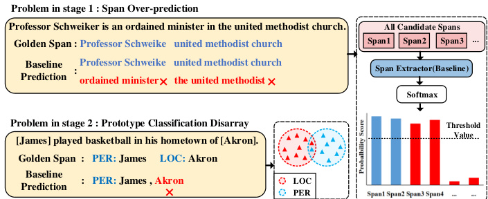
Figure 1: The illustration of the baseline model suffering from span over-prediction (upper) and Prototype Classification Disarray (down) problem in few-shot NER.
图 1: 少样本NER中基线模型遭遇跨度过度预测(上)和原型分类混乱(下)问题的示意图。
To tackle these limitations, we propose a Multi-Task Semantic Decomposition Framework via Joint Task-specific Pre-training (MSDP), which guides PLMs to capture reliable entity boundary information and better entity representations of different classes. For the pre-training stage, inspired by demonstration-based learning [19] and contrastive learning [9], we introduce two novel taskspecific pre-training tasks according to the data characteristics of NER (entity-label pairs): Demonstration-based MLM, in which we design three kinds of demonstrations containing entity boundary information and entity label pair information. PLMs will implicitly learn the above information during predicting label words for [MASK]; Class Contrastive Discrimination, in which we use contrastive learning to better discriminate different classes of entity representations by constructing positive, negative, and hard negative samples. Through the joint optimization of above fine-grained pre-training tasks, PLMs can effectively alleviate the two remaining problems.
为解决这些局限性,我们提出了一种通过联合任务特定预训练 (MSDP) 实现的多任务语义分解框架,该框架指导预训练语言模型 (PLM) 捕获可靠的实体边界信息以及不同类别的更优实体表示。在预训练阶段,受基于演示的学习 [19] 和对比学习 [9] 启发,我们根据命名实体识别 (NER) 的数据特性(实体-标签对)设计了两个新颖的任务特定预训练任务:基于演示的掩码语言建模 (Demonstration-based MLM)——通过设计三种包含实体边界信息和实体标签对信息的演示样本,使 PLM 在预测[MASK]标签词时隐式学习上述信息;类别对比判别 (Class Contrastive Discrimination)——通过构建正样本、负样本和困难负样本,利用对比学习更好地区分不同类别的实体表示。通过对上述细粒度预训练任务的联合优化,PLM 能有效缓解剩余的两个问题。
For downstream few-shot NER, we follow the two-stage framework [47, 65] including span extraction and entity classification, and initialize them with the pre-trained parameters. Different from previous methods, we employ a multi-task joint optimization framework and utilize different masking strategies to decompose class-oriented prototypes and contextual fusion prototypes. The purpose of our design is to assist the model to integrate different semantic information for classification, which further alleviates the prototype classification disarray problem. We conduct extensive experiments over two widely-used benchmarks, including Few-NERD [14] and CrossNER [28]. Results show that our method consistently outperforms state-of-the-art baselines by a large margin. In addition, we introduce detailed experimental analyses to further verify the effectiveness of our method. Our contributions are three-fold:
在下游少样本命名实体识别(NER)任务中,我们采用包含跨度提取和实体分类的两阶段框架[47,65],并使用预训练参数进行初始化。与现有方法不同,我们采用多任务联合优化框架,并运用不同的掩码策略来分解面向类别的原型和上下文融合原型。该设计旨在帮助模型整合不同语义信息进行分类,从而进一步缓解原型分类混乱问题。我们在Few-NERD[14]和CrossNER[28]这两个广泛使用的基准测试上进行了大量实验。结果表明,我们的方法始终以较大优势超越现有最优基线模型。此外,我们还通过详细的实验分析进一步验证了方法的有效性。本文主要贡献包括以下三个方面:
- To the best of our knowledge, we are the first to introduce a multitask joint optimization framework with the semantic decomposing method into Few-Shot NER task.
- 据我们所知,我们是首个将多任务联合优化框架与语义分解方法引入少样本命名实体识别 (Few-Shot NER) 任务的团队。
- we futher propose two task-specific pre-training tasks via demonstration and contrastive learning, namely demonstration-based MLM and class contrastive discrimination, for effectively injecting entity boundary information and better entity representation into PLMs.
- 我们进一步提出两种基于演示和对比学习的任务特定预训练任务,即基于演示的MLM(Masked Language Model)和类别对比判别,以有效将实体边界信息和更优的实体表征注入预训练语言模型(PLMs)。
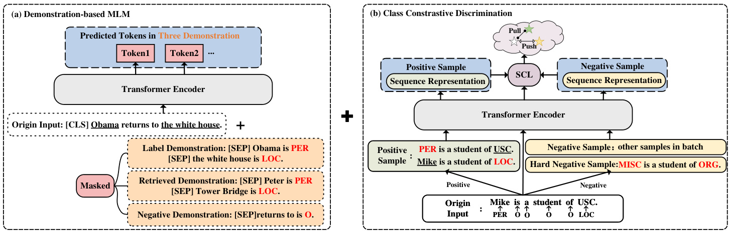
Figure 2: The illustration of two task-specific pre-training tasks.
图 2: 两种任务特定预训练任务的示意图。
- Experiments on two widely-used few-shot NER benchmarks show that our framework achieves superior performance over previous state-of-the-art methods. Extensive analyses further validate the effectiveness and generalization of MSDP. Our source codes and datasets are available at Github for further comparisons.
- 在两个广泛使用的少样本命名实体识别(NER)基准测试上的实验表明,我们的框架优于之前最先进的方法。大量分析进一步验证了MSDP的有效性和泛化能力。我们的源代码和数据集已发布在Github上以供进一步比较。
2 RELATED WORK
2 相关工作
2.1 Few-shot NER.
2.1 少样本命名实体识别 (Few-shot NER)
Few-shot NER aims to enhance the performance of model identifying and classifying entities with only little annotated data [7, 21, 30, 31, 38, 42–45, 62, 77]. For few-shot NER, a series of approaches have been proposed to learn the representation of entities in the semantic space, i.e. prototypical learning [59], margin-based learning [36] and contrastive learning [20, 24, 37]. Existing approaches can be divided into two kinds, i.e., one-stage [11, 28, 59, 81] and two-stage [16, 47, 58, 69]. Generally, the methods in the kind of one-stage typically categorize the entity type by token-level metric learning. In contrast, two-stage mainly focuses on two training stages consisting of entity span extraction and mention type classification.
少样本NER (Few-shot NER) 旨在通过少量标注数据提升模型识别和分类实体的性能 [7, 21, 30, 31, 38, 42–45, 62, 77]。针对少样本NER,研究者提出了一系列方法来学习实体在语义空间中的表示,例如原型学习 (prototypical learning) [59]、基于间隔的学习 (margin-based learning) [36] 和对比学习 (contrastive learning) [20, 24, 37]。现有方法可分为两类:单阶段 (one-stage) [11, 28, 59, 81] 和双阶段 (two-stage) [16, 47, 58, 69]。通常,单阶段方法通过token级度量学习直接分类实体类型,而双阶段方法则包含实体范围抽取和提及类型分类两个训练阶段。
2.2 Task-specific pre-training Models.
2.2 任务特定预训练模型
Pre-trained language models have been applied as an integral component in modern NLP systems for effectively improving downstream tasks [13, 40, 52, 54, 55, 71, 74, 76]. Due to the underlying discrepancies between the language modeling and downstream tasks, task-specific pre-training methods have been proposed to further boost the task performance, such as SciBERT [5], VideoBERT [61], DialoGPT [75], PLATO [4], Code-BERT [17], ToD-BERT [68] and VL-BERT [60]. However, most studies in the field of few-shot NER use MLM and other approaches for Data Augmentation [15, 29, 79]. Although DictBERT [8], NER-BERT [41] and others have conducted pre-training, their methods are too generalized to adapt to the structured data features of NER or propose optimization for specific problems. Therefore, we designed demonstration-based learning pre-training and contrastive learning pre-training for NER tasks to improve the performance of the model.
预训练语言模型已成为现代自然语言处理(NLP)系统的核心组件,能有效提升下游任务性能 [13, 40, 52, 54, 55, 71, 74, 76]。由于语言建模任务与下游任务存在本质差异,研究者提出了面向特定任务的预训练方法以进一步提升性能,例如 SciBERT [5]、VideoBERT [61]、DialoGPT [75]、PLATO [4]、Code-BERT [17]、ToD-BERT [68] 和 VL-BERT [60]。然而当前少样本命名实体识别(NER)领域的研究大多采用掩码语言建模(MLM)等数据增强方法 [15, 29, 79]。虽然 DictBERT [8]、NER-BERT [41] 等模型进行了预训练,但其方法过于通用化,既未适配NER任务的结构化数据特征,也未针对具体问题提出优化方案。为此,我们设计了基于示例学习的NER预训练方法和对比学习预训练方法以提升模型性能。
2.3 Demonstration-based learning
2.3 基于演示的学习
Demonstrations are first introduced by the GPT series [6, 55], where a few examples are sampled from training data and transformed with templates into appropriately-filled prompts. Based on the task reformulation and whether the parameters are updated, the existing demonstration-based learning research can be broadly divided into three categories: In-context Learning [6, 48, 67, 78], Prompt-based Fine-tuning [39], Classifier-based Fine-tuning [35, 72]. However, these approaches mainly adopt demonstration-based learning in the fine-tuning that cannot make full use of the effect of demonstrationbased learning. Different from them, we use demonstration-based learning in the pre-training stage that can better capture the entity boundary information to solve the multiple-span prediction problem.
演示学习最初由GPT系列[6,55]提出,该方法从训练数据中采样少量示例,并通过模板将其转换为填充得当的提示词。根据任务重构方式和参数是否更新,现有基于演示学习的研究可大致分为三类:上下文学习[6,48,67,78]、基于提示的微调[39]、基于分类器的微调[35,72]。然而这些方法主要在微调阶段采用演示学习,无法充分发挥演示学习的效用。与之不同,我们将演示学习应用于预训练阶段,从而更好地捕捉实体边界信息以解决多跨度预测问题。
3 METHOD
3 方法
3.1 Task-Specific Pre-training
3.1 任务特定预训练
The performance of few-shot NER depends heavily on the different aspects of information from entity label pairs. as shown in Figure 2, we introduce two novel pre-training tasks: 1) demonstration-based MLM and 2) contrastive entity discrimination, to learn the different aspects of knowledge.
少样本NER (Named Entity Recognition) 的性能在很大程度上依赖于来自实体标签对的不同方面信息。如图 2 所示,我们引入了两种新颖的预训练任务: 1) 基于演示的MLM (Masked Language Modeling) 和 2) 对比实体判别,以学习不同方面的知识。
Demonstration-based MLM. We follow the design of masked language modeling (MLM) in BERT [13] and integrate the idea of demonstration-based learning on this basis. In order to prompt PLMs to figure out the boundary between the entity and noneentity, we propose three different demonstrations which are shown in Figure 2(a):
基于演示的MLM。我们遵循BERT [13]中掩码语言建模(MLM)的设计,并在此基础上整合了基于演示学习的思想。为了促使预训练语言模型(PLM)区分实体与非实体的边界,我们提出了三种不同的演示方案,如图2(a)所示:
- Label demonstration (LD): We let $D_{t r a i n}$ denote the train dataset. For each input $x$ in $D_{t r a i n}$ , we extract the entity label pair $(e,l)$ belonging to $x$ and then concatenate them behind input $x$ in form of the simple template $T={e$ 𝑖𝑠 $l}$ . Different demonstrations are separated by [SEP].
- 标签演示 (LD):我们用 $D_{train}$ 表示训练数据集。对于 $D_{train}$ 中的每个输入 $x$,我们提取属于 $x$ 的实体标签对 $(e,l)$,然后按照简单模板 $T={e$ 𝑖𝑠 $l}$ 的形式将它们拼接在输入 $x$ 后面。不同的演示之间用 [SEP] 分隔。
- Retrieved demonstration (RD): Given an entity type label set $L={l_{1},...,l_{|L|}}$ , we first enumerate all the entities in $D_{t r a i n}$ and create a mapping between $l$ and the corresponding list of entities. Further, we randomly select $K$ entity label pairs $(e,l)$ from the mapping $M$ according to the label set $L_{x}$ appearing in input $x$ , which aims at introducing rich entity label pair information to prompt the model. Furthermore, we concatenate them behind label demonstration with template $T={e i s l}$ .
- 检索演示 (Retrieved Demonstration, RD):给定实体类型标签集 $L={l_{1},...,l_{|L|}}$,我们首先枚举 $D_{train}$ 中的所有实体,并创建映射关系 。接着,根据输入 $x$ 中出现的标签集 $L_{x}$,从映射 $M$ 中随机选取 $K$ 个实体标签对 $(e,l)$,旨在向模型引入丰富的实体标签对信息。最后,我们使用模板 $T={e\ is\ l}$ 将这些实体标签对拼接在标签演示之后。
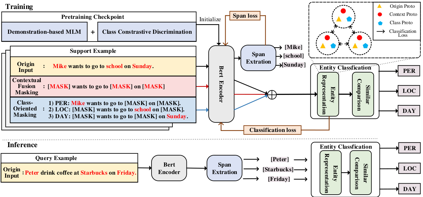
Figure 3: The overall architecture of our proposed MSDP framework
图 3: 我们提出的 MSDP 框架整体架构
- Negative demonstration (ND): We randomly select $K$ noneentities that are easily confused by the model from input $x$ to construct negative sample pairs $(e_{n o n e},O)$ , and then concatenate them behind retrieved demonstrations with template $T^{\prime}={e_{n o n e}$ 𝑖𝑠 $O}$ . Therefore, our training samples can be formulated as:
- 负例演示(ND): 我们从输入$x$中随机选取$K$个容易被模型混淆的非实体(noneentities),构建负样本对$(e_{none},O)$,然后用模板$T^{\prime}={e_{none}$ is $O}$将它们拼接在检索到的演示之后。因此,我们的训练样本可以表示为:
$$
\left[\mathsf{C L S}\right]x\left[\mathsf{S E P}\right]L D\left[\mathsf{S E P}\right]R D\left[\mathsf{S E P}\right]N D
$$
$$
\left[\mathsf{C L S}\right]x\left[\mathsf{S E P}\right]L D\left[\mathsf{S E P}\right]R D\left[\mathsf{S E P}\right]N D
$$
After constructing the training set, we randomly randomly replace N entities or labels with mask symbols or labels in the demonstration with the special $I M A S K J{s y m b o l}^{2}$ , and then try to recover them. If entity $e$ consists of multiple tokens, all of the component tokens will be masked. Hence, the loss function of the MLM is:
在构建训练集后,我们随机将演示中的N个实体或标签替换为特殊符号 $I M A S K J{s y m b o l}^{2}$ 的掩码符号或标签,然后尝试恢复它们。如果实体 $e$ 由多个token组成,则所有组成token都将被掩码。因此,MLM (Masked Language Model) 的损失函数为:
$$
L_{m l m}=-\sum_{m=1}^{M}\log P(x_{m})
$$
$$
L_{m l m}=-\sum_{m=1}^{M}\log P(x_{m})
$$
where $M$ is the total number of masked tokens and $P(x_{m})$ is the predicted probability of the token $x_{m}$ over the vocabulary size.
其中 $M$ 是被遮蔽 token 的总数,$P(x_{m})$ 是 token $x_{m}$ 在词汇表大小上的预测概率。
Class Contrastive Discrimination. To better discriminate different classes of entity representations in semantic space, we introduce class contrastive discrimination. Specifically, we construct positive (negative) samples as follows:
类别对比判别。为了更好地在语义空间中区分不同类别的实体表征,我们引入了类别对比判别方法。具体而言,我们按以下方式构建正(负)样本:
Given an input $x$ that contains $K$ entities, we employ the following procedure to generate positive and negative samples. For positive samples, we replace these $K$ entities with their corresponding label mentions to create $K$ positive samples for each input utterance. For negative samples, we select samples from other classes within the batch. Additionally, we replace all entities with irrelevant label mentions to construct a hard negative sample for each instance that is easily confused by the model. These hard negative samples are then included in the negative sample set. Figure 2 illustrates the corresponding positive and negative samples as depicted in our experiment.
给定一个包含 $K$ 个实体的输入 $x$,我们采用以下流程生成正负样本。对于正样本,我们将这 $K$ 个实体替换为对应的标签提及,从而为每个输入语句创建 $K$ 个正样本。对于负样本,我们从批次内的其他类别中选取样本。此外,我们将所有实体替换为不相关的标签提及,为每个容易被模型混淆的实例构建一个困难负样本,并将这些困难负样本纳入负样本集。图 2 展示了我们实验中对应的正负样本示例。
The representations of the original, positive, and negative samples are denoted by $h_{o},h_{p}$ , and $h_{n}$ , respectively. To account for multiple positive samples, we adopt the supervised contrastive learning (SCL) objective [32], which aims to minimize the distance between the original samples $h_{o}$ and their semantically similar positive samples $h_{p}$ , while maximizing the distance between $h_{o}$ and 2 samples: the negative samples $h_{n}$ and the hard negative samples $h_{h n}$ . The formulation of $L_{S C L}$ is as follow:
原始样本、正样本和负样本的表示分别记为 $h_{o},h_{p}$ 和 $h_{n}$。为处理多正样本情况,我们采用监督对比学习 (supervised contrastive learning, SCL) 目标函数 [32],其核心是最小化原始样本 $h_{o}$ 与语义相似的正样本 $h_{p}$ 之间的距离,同时最大化 $h_{o}$ 与两类样本的距离:负样本 $h_{n}$ 和困难负样本 $h_{h n}$。$L_{S C L}$ 的公式如下:
$$
\begin{array}{l}{\displaystyle\mathcal{L}{S C L}=\frac{-1}{N}\sum_{i=1}^{N}{\frac{1}{N_{y_{i}}}\sum_{j=1}^{N_{y_{i}}}\sum_{k=1}^{N_{y_{i}}}\mathbb{I}{y_{i j}=y_{i k}}}}\ {\displaystyle\log\frac{e^{s i m(h_{o i j},h_{p i k})/\tau}}{\sum_{l=1}^{N}(\mathbb{I}{j\neq l})e^{s i m(h_{o i j},h_{n l})/\tau}+e^{s i m(h_{o i j},h_{h n i j})/\tau}}}\end{array}
$$
$$
\begin{array}{l}{\displaystyle\mathcal{L}{S C L}=\frac{-1}{N}\sum_{i=1}^{N}{\frac{1}{N_{y_{i}}}\sum_{j=1}^{N_{y_{i}}}\sum_{k=1}^{N_{y_{i}}}\mathbb{I}{y_{i j}=y_{i k}}}}\ {\displaystyle\log\frac{e^{s i m(h_{o i j},h_{p i k})/\tau}}{\sum_{l=1}^{N}(\mathbb{I}{j\neq l})e^{s i m(h_{o i j},h_{n l})/\tau}+e^{s i m(h_{o i j},h_{h n i j})/\tau}}}\end{array}
$$
where $N$ and $N_{y_{i}}$ denote the number of total examples in the batch and positive samples. $\tau$ is a temperature hyper parameter and $s i m(h_{1},h_{2})$ is cosine similarity. 1 is an indicator function.
其中 $N$ 和 $N_{y_{i}}$ 分别表示批次中的总样本数和正样本数。$\tau$ 是温度超参数,$sim(h_{1},h_{2})$ 为余弦相似度。1 是指示函数。
We sum the demonstration-base MLM task loss and the class contrastive discrimination task loss, and finally obtain the overall loss function L:
我们将基于演示的MLM任务损失和类别对比判别任务损失相加,最终得到整体损失函数L:
$$
L=\alpha L_{m l m}+(1-\alpha)L_{S C L}
$$
$$
L=\alpha L_{m l m}+(1-\alpha)L_{S C L}
$$
where $L_{m l m}$ and $L_{c}$ denote the loss functions of the two tasks. In our experiments, we set $\alpha=0.6$ .
其中 $L_{m l m}$ 和 $L_{c}$ 表示两个任务的损失函数。在我们的实验中,设置 $\alpha=0.6$。
3.2 Downstream Few-shot NER
3.2 下游少样本命名实体识别
After the pre-training stage, our model initially learns different aspects of information. In this section, We formally present the notations and the techniques of our proposed MSDP in the finetuning stage. Figure 3 illustrates the overall framework, which is composed of two steps: span extraction and entity classification.
在预训练阶段之后,我们的模型初步学习了信息的不同方面。本节正式介绍微调阶段提出的MSDP (Multi-Step Dynamic Pretraining) 符号体系和技术方案。图3展示了整体框架,该框架由两个步骤组成:跨度提取和实体分类。
3.2.1 Notations. We denote the train and test sets by $\mathcal{D}{t r a i n}$ and $\mathcal{D}{t e s t}$ , respectively. Both of them have the form of meta-learning datasets. The dataset consists of multiple episodes of data, and each episode of data ${\mathcal{E}}=(S,Q)$ consists of a support set $s$ and a query set $\boldsymbol{\mathcal{Q}}$ . A sample $(X,y)$ in the support set or query set consists of the input sentence $X$ and the label set $\mathcal{Y}=\bar{{(s_{j},e_{j},y_{j})}}{j=1}^{N}$ (𝑁 denoting the number of spans, $s_{j}$ and $e_{j}$ denoting the start and end positions of the $j$ -th span, $y_{j}$ denoting the category of the $j$ -th span). $\pmb{h}$ denotes the hidden representation obtained by encoding the input text.
3.2.1 符号说明。我们将训练集和测试集分别表示为 $\mathcal{D}{train}$ 和 $\mathcal{D}{test}$。两者均采用元学习数据集的形式,该数据集由多个数据片段组成,每个数据片段 ${\mathcal{E}}=(S,Q)$ 包含支持集 $s$ 和查询集 $\boldsymbol{\mathcal{Q}}$。支持集或查询集中的样本 $(X,y)$ 由输入句子 $X$ 和标签集 $\mathcal{Y}=\bar{{(s_{j},e_{j},y_{j})}}{j=1}^{N}$ 构成(其中 𝑁 表示跨度数量,$s_{j}$ 和 $e_{j}$ 表示第 $j$ 个跨度的起止位置,$y_{j}$ 表示第 $j$ 个跨度的类别)。$\pmb{h}$ 表示通过编码输入文本获得的隐藏表示。
3.2.2 Span Extractor. The span extractor aims to detect all entity spans. We initialize encoder with pre-trained parameters to encode the input sentence as a hidden representation $\pmb{h}$ , and calculate attention scores between each token representation to judge the start token and end token of the entity span. Following previous works [47, 65], we use span-based cross-entropy as the loss function to optimise our encoder. We first design the weight matrixes $W_{q}/W_{k}/W_{v}$ of values $q/k/v$ and bias $b_{q}/b_{k}$ for the attention mechanism, and then compute the attention score of the $i$ -th and $j$ -th token, using formula: $f(i,j)=q_{i}^{T}k_{j}+W_{v}({h}{i}+{h}{j}).\Omega_{i,j}$ indicates whether the span bounded by 𝑖, $j$ is an entity. Therefore, the span-based cross-entropy can be expressed as:
3.2.2 跨度提取器。跨度提取器旨在检测所有实体跨度。我们使用预训练参数初始化编码器,将输入句子编码为隐藏表示 $\pmb{h}$,并通过计算每个token表示之间的注意力分数来判断实体跨度的起始token和结束token。遵循先前工作[47,65],我们采用基于跨度的交叉熵作为损失函数来优化编码器。首先为注意力机制设计值 $q/k/v$ 的权重矩阵 $W_{q}/W_{k}/W_{v}$ 和偏置 $b_{q}/b_{k}$,然后通过公式计算第 $i$ 个与第 $j$ 个token的注意力分数:$f(i,j)=q_{i}^{T}k_{j}+W_{v}({h}{i}+{h}{j})$。$\Omega_{i,j}$ 表示由 𝑖 和 $j$ 界定的跨度是否为实体,因此基于跨度的交叉熵可表示为:
$$
\mathcal{L}{s p a n}=\log(1+\sum_{1\leq i<j\leq L}\exp((-1)^{\Omega_{i,j}}f(i,j))
$$
$$
\mathcal{L}{s p a n}=\log(1+\sum_{1\leq i<j\leq L}\exp((-1)^{\Omega_{i,j}}f(i,j))
$$
3.2.3 Entity Classification. In the second stage, we classify the entity spans extracted in the first stage. Different from the previous methods only computing the original prototype, we further decompose class-oriented prototypes and contextual fusion prototypes by two masking strategies, which introduce different information to assist in the classification task, thus alleviating the prototype classification disarray problem.
3.2.3 实体分类。在第二阶段,我们对第一阶段提取的实体跨度进行分类。与之前仅计算原始原型的方法不同,我们通过两种掩码策略进一步分解面向类别的原型和上下文融合原型,这些策略引入了不同信息来辅助分类任务,从而缓解原型分类混乱问题。
- Semantic masking strategies. Firstly, we introduce two novel semantic masking strategies for the subsequent construction of semantic decomposing prototypes.
- 语义掩码策略。首先,我们为后续构建语义分解原型引入两种新颖的语义掩码策略。
• Class-oriented Masking: Given an input sentence $X={x_{1},x_{2}$ , $\dots,x_{L}}$ , we replace all the entity spans in $X$ whose labels that are not $y$ with [MASK] tokens to obtain class $y$ specific input $X_{\mathrm{cs}}^{y}$ , thereby forcing the model to focus on the information of specific class by shielding the interference of other entities. For example, as shown in Figure 3, we replace the “school” entity of the “LOC” class and the “Sunday” entity of the “DAY” class with [MASK] tokens to obtain “PER” class-oriented input Mike wants to go to [MASK] on [MASK].
• 面向类别的掩码处理:给定输入句子 $X={x_{1},x_{2}$ , $\dots,x_{L}}$ ,我们将 $X$ 中所有标签不为 $y$ 的实体跨度替换为[MASK]标记,从而获得类别 $y$ 的特定输入 $X_{\mathrm{cs}}^{y}$ ,通过屏蔽其他实体的干扰迫使模型专注于特定类别的信息。例如,如图 3 所示,我们将"LOC"类别的"school"实体和"DAY"类别的"Sunday"实体替换为[MASK]标记,得到面向"PER"类别的输入 Mike wants to go to [MASK] on [MASK]。
• Contextual Fusion Masking: we replace all the entities in a sentence with [MASK] tokens, thus allowing the model to focus more on contextual fusion information. As the example sentence in Figure 3, we mask all entities to obtain $X_{\mathrm{ctx}}=$ [MASK] wants to go to [MASK] on [MASK].
• 上下文融合掩码 (Contextual Fusion Masking):我们将句子中的所有实体替换为[MASK] token,从而使模型更专注于上下文融合信息。如图 3 中的示例句子所示,我们掩码所有实体得到 $X_{\mathrm{ctx}}=$ [MASK] wants to go to [MASK] on [MASK]。
- Prototype Constructing. After decomposing two types of inputs with different information, we construct original prototype and two extra prototypes for each class in entity classification stage (The upper right corner of Figure 3)
- 原型构建。在分解两类不同信息的输入后,我们为实体分类阶段的每个类别构建原始原型和两个额外原型 (图 3 右上角)
For original prototype, we add up the representations of the start token and the end token of an entity span as the span boundary representation:
对于原始原型,我们将实体跨度的起始token和结束token的表示相加作为跨度边界表示:
$$
{\pmb u}{j}={\pmb h}{s_{j}}+{\pmb h}{e_{j}}
$$
$$
{\pmb u}{j}={\pmb h}{s_{j}}+{\pmb h}{e_{j}}
$$
where $\pmb{u}{j}$ is the representation of the $j$ -th span in the sentence, $\pmb{h}{i}$ denote the representation of the $i$ -th token in the sentence. $s_{j}$ and $e_{j}$ are the start and end positions of the $j$ -th span respectively.
其中 $\pmb{u}{j}$ 表示句中第 $j$ 个片段 (span) 的表征,$\pmb{h}{i}$ 表示句中第 $i$ 个 token 的表征。$s_{j}$ 和 $e_{j}$ 分别表示第 $j$ 个片段的起始位置和结束位置。
For class-oriented prototype, we perform a class-oriented masking strategy for class $t$ on $X$ to obtain $X_{\mathrm{cs}}^{\mathrm{t}}$ , and compute a span representation ${\pmb u}{j}^{\mathrm c s}$ in $X_{\mathrm{c}s}^{\mathrm{t}}$ according to equation 6.
针对类别导向的原型方法,我们对类别 $t$ 在 $X$ 上执行类别导向掩码策略以获得 $X_{\mathrm{cs}}^{\mathrm{t}}$ ,并根据公式6计算 $X_{\mathrm{c}s}^{\mathrm{t}}$ 中的跨度表示 ${\pmb u}_{j}^{\mathrm c s}$ 。
For contextual fusion prototype, we perform all the entity-masking strategy on the original sentence $X$ to obtain $X_{\mathrm{ctx}}$ and then compute the span representation ${\pmb u}_{j}^{\mathrm{ctx}}$ by averaging the representations of all tokens as follow:
对于上下文融合原型,我们在原始句子$X$上执行所有实体掩码策略以获得$X_{\mathrm{ctx}}$,然后通过平均所有token的表示来计算跨度表示${\pmb u}_{j}^{\mathrm{ctx}}$,如下所示:
$$
u_{j}^{\mathrm{ctx}}=\frac{1}{L}\sum_{i=1}^{L}h_{i}
$$
$$
u_{j}^{\mathrm{ctx}}=\frac{1}{L}\sum_{i=1}^{L}h_{i}
$$
where $L$ denotes the number of tokens in $X_{\mathrm{ctx}}$
其中 $L$ 表示 $X_{\mathrm{ctx}}$ 中的 token 数量
Afterwards, we construct three different prototypes vectors by averaging the representations of all entities of the same class in the support set:
随后,我们通过在支持集中对所有同类实体的表征进行平均,构建了三种不同的原型向量:
$$
\pmb{c}{t}=\frac{\sum_{(X,y)\in S}\sum_{(s_{j},e_{j},y_{j})\in\pmb{y}}\mathbb{I}(y_{j}=t)\pmb{u}}{\sum_{(X,y)\in S}\sum_{(s_{j},e_{j},y_{j})\in\pmb{y}}\mathbb{I}(y_{j}=t)}
$$
$$
\pmb{c}{t}=\frac{\sum_{(X,y)\in S}\sum_{(s_{j},e_{j},y_{j})\in\pmb{y}}\mathbb{I}(y_{j}=t)\pmb{u}}{\sum_{(X,y)\in S}\sum_{(s_{j},e_{j},y_{j})\in\pmb{y}}\mathbb{I}(y_{j}=t)}
$$
where $\mathbb{I}(\cdot)$ is the indicator function; $\pmb{u}$ can be replaced with $\pmb{u}{j}$ ${\pmb u}{j}^{\mathrm c s}$ and ${\pmb u}_{j}^{\mathrm{ctx}}$ to calculate three semantic prototypes separately.
其中 $\mathbb{I}(\cdot)$ 是指示函数;$\pmb{u}$ 可替换为 $\pmb{u}{j}$、${\pmb u}{j}^{\mathrm c s}$ 和 ${\pmb u}_{j}^{\mathrm{ctx}}$ 以分别计算三个语义原型。
After constructing three different semantic prototypes, we use a metric-based approach for classification and optimize the parameters of the model based on the basis of distance between entity representations and class prototypes:
在构建了三种不同的语义原型后,我们采用基于度量的方法进行分类,并根据实体表示与类原型之间的距离优化模型参数:
$$
\mathcal{L}{c l s}=\sum_{(X,y)\in S}\sum_{(s_{j},e_{j},y_{j})\in\mathcal{Y}}-\log\mathcal{p}(y_{j}|s_{j},e_{j})
$$
$$
\mathcal{L}{c l s}=\sum_{(X,y)\in S}\sum_{(s_{j},e_{j},y_{j})\in\mathcal{Y}}-\log\mathcal{p}(y_{j}|s_{j},e_{j})
$$
where
其中
$$
\begin{array}{r}{\quad p(y_{j}|s_{j},e_{j})=\mathrm{softmax}(-d(\pmb{u}{j},\pmb{c}{y_{j}}))}\end{array}
$$
$$
\begin{array}{r}{\quad p(y_{j}|s_{j},e_{j})=\mathrm{softmax}(-d(\pmb{u}{j},\pmb{c}{y_{j}}))}\end{array}
$$
is the probability distribution. We use cosine similarity as the distance function $d(\cdot,\cdot)$ .
概率分布为。我们使用余弦相似度作为距离函数 $d(\cdot,\cdot)$。
3.3 Training and Inference of MSDP
3.3 MSDP的训练与推理
We first perform two task-specific pre-trainings to learn reliable entity boundary information and entity representations of different classes. For fine-tuning, we initialize the BERT encoder with pretrained parameters for the few-shot NER task.
我们首先进行两项任务特定的预训练,以学习可靠的实体边界信息和不同类别的实体表示。在微调阶段,我们使用预训练参数初始化BERT编码器,用于少样本命名实体识别任务。
In the downstream training phase, given the training set $\mathcal{D}{t r a i n}=$ $(S,Q)$ , we compute $\mathcal{L}{s p a n}$ and three types of prototypes on the support set $s$ , $\mathcal{L}{c l s}$ on the query set $\boldsymbol{\mathcal{Q}}$ , and train the two optimization objectives jointly. Following SpanProto [65], we only optimize the $\mathcal{L}{s p a n}$ objective in the first $T$ steps, and jointly optimize both $\mathcal{L}{s p a n}$ and $\mathcal{L}_{c l s}$ after $T$ steps.
在下游训练阶段,给定训练集 $\mathcal{D}{train}=$ $(S,Q)$,我们在支持集 $s$ 上计算 $\mathcal{L}{span}$ 和三种原型,在查询集 $\boldsymbol{\mathcal{Q}}$ 上计算 $\mathcal{L}{cls}$,并联合训练这两个优化目标。遵循 SpanProto [65] 的方法,我们仅在初始 $T$ 步优化 $\mathcal{L}{span}$ 目标,之后 $T$ 步开始联合优化 $\mathcal{L}{span}$ 和 $\mathcal{L}_{cls}$。
Table 1: Evaluation dataset statistics.
| 数据集 | 领域 | 句子数 | 类别数 |
|---|---|---|---|
| Few-NERD | Wikipedia | 188.2k | 66 |
| CoNLL03 | 新闻 | 20.7k | 4 |
| GUM | Wiki | 3.5k | 11 |
| WNUT | 社交媒体 | 5.6k | 6 |
| OntoNotes | 混合 | 159.6k | 18 |
表 1: 评估数据集统计。
In the testing phase, given an episode $\mathcal{E}=(S,Q)\in\mathcal{D}_{t e s t}$ , we construct prototypes on the support set $s$ and perform span detection on the query set $\boldsymbol{\alpha}$ . Then we calculate the distance between the extracted spans and each class prototype for classification. Note that we only utilize original prototypes during inference.
在测试阶段,给定一个情节 $\mathcal{E}=(S,Q)\in\mathcal{D}_{t e s t}$,我们在支持集 $s$ 上构建原型,并在查询集 $\boldsymbol{\alpha}$ 上执行跨度检测。然后计算提取的跨度与每个类原型之间的距离以进行分类。请注意,在推理过程中我们仅使用原始原型。
4 EXPERIMENT
4 实验
4.1 Datasets
4.1 数据集
Table 1 shows the dataset statistics of original data for constructing few-shot episodes. We evaluate our method on two widely used few-shot benchmarks Few-NERD [14] and CrossNER [45].
表 1: 展示了用于构建少样本 (few-shot) 任务的原始数据集统计信息。我们在两个广泛使用的少样本基准测试 Few-NERD [14] 和 CrossNER [45] 上评估了我们的方法。
Few-NERD: Few-NERD is annotated with 8 coarse-grained and 66 fine-grained entity types, which consists of two few-shot settings (Intra, and Inter). In the Intra setting, all entities in the training set, development set, and testing set belong to different coarse-grained types. In contrast, in the Inter setting, only the fine-grained entity types are mutually disjoint in different datasets. we use episodes released by Ding et al. which contains 20,000 episodes for training, 1,000 episodes for validation, and 5,000 episodes for testing. Each episode is an $N$ -way $K\sim2K$ -shot few-shot task.
Few-NERD:Few-NERD标注了8个粗粒度与66个细粒度实体类型,包含两种少样本设定(Intra和Inter)。在Intra设定中,训练集、开发集和测试集的所有实体均属于不同粗粒度类型;而在Inter设定中,仅要求不同数据集的细粒度实体类型互不相交。我们采用Ding等人发布的20,000个训练片段、1,000个验证片段和5,000个测试片段,每个片段均为$N$元$K\sim2K$样本的少样本任务。
CrossNER: CrossNER contains four domains from CoNLL-2003 57, GUM [73] (Wiki), WNUT-2017 [12] (Social), and Ontonotes 53. We randomly select two domains for training, one for validation, and the remaining for testing. We use public episodes constructed by Hou et al. .
CrossNER:CrossNER包含来自CoNLL-2003 [57](新闻)、GUM [73](维基)、WNUT-2017 [12](社交)和Ontonotes [53](混合)的四个领域。我们随机选择两个领域进行训练,一个用于验证,其余用于测试。我们使用Hou等人构建的公共片段。
4.2 Baselines
4.2 基线方法
For the baselines, we choose multiple strong approaches from the paradigms of one-stage and two-stage. 1) One-stage NER paradigms: ProtoBERT [59], StructShot [70], NNShot [70], CONTAINER [11] and LTapNet $^+$ CDT [28]. 2) Two-stage paradigm: ESD [66], MAML- ProtoNet [47] and SpanProto [65]. Due to the space limitation, More details of these baselines and implementations are illustrated as follow:
在基线模型选择上,我们分别从单阶段和双阶段范式中选取了多种强效方法:1) 单阶段命名实体识别范式:ProtoBERT [59]、StructShot [70]、NNShot [70]、CONTAINER [11] 以及 LTapNet$^+$CDT [28];2) 双阶段范式:ESD [66]、MAML-ProtNet [47] 和 SpanProto [65]。由于篇幅限制,这些基线模型及实现细节如下所示:
• SimBERT [28] applies BERT without any finetuning as the embedding function, then assigns each token’s label by retrieving the most similar token in the support set. • ProtoBERT [18] uses a token- level prototypical network [59] which represents each class by averaging token representations with the same label, then the label of each token in the query set is decided by its nearest class prototype.
• SimBERT [28] 直接使用未经微调的 BERT 作为嵌入函数,然后通过在支持集中检索最相似的 token 来分配每个 token 的标签。
• ProtoBERT [18] 采用 token 级别的原型网络 [59],通过平均具有相同标签的 token 表示来表征每个类别,然后查询集中每个 token 的标签由其最近的类别原型决定。
4.3 Implementation Detail
4.3 实现细节
For the upstream work, we use BERT-base-uncased [13] from HuggingFace as the backbone. In two pre-training settings, we set the batch size of BERT to 8 and the pre-training takes an average of 12 hours for 5 epochs. The corresponding learning rates are set to 1e-5. We set the number (K) of the retrieved demonstrations to 5 and the negative demonstration to 3. We set temperature hyper parameter $\tau_{1}$ to 0.5. In addition, our upstream pre-training corpus is aligned with the downstream task, which means no additional data will be introduced in the pre-training stage. For instance, if the downstream few-shot NER experiment is conducted on the Inter 5 way 1-2 shot of Few-NERD, the pre-training data is the training set of Inter 5 way 1-2 shot.
在上游工作中,我们采用HuggingFace的BERT-base-uncased [13]作为主干模型。在两种预训练设置中,将BERT的批处理大小设为8,5个epoch的平均预训练时长为12小时,对应学习率设置为1e-5。检索演示样本数(K)设为5,负样本数设为3,温度超参数$\tau_{1}$设为0.5。此外,上游预训练语料与下游任务对齐,意味着预训练阶段不会引入额外数据。例如,若下游少样本NER实验在Few-NERD的Inter 5 way 1-2 shot数据集上进行,则预训练数据即为该数据集的训练集。
For the downstream work, we adopt the standard N-way K-shot setting [14] and align the task definition with previous work [47]. We choose Adam [33] as the optimizer with a learning rate of 3e-5. The warm-up rate is set to 0.1. The max sequence length we set is 64 and the batch size is set to 4. The training steps T and T’ are set as 2000 and 200, respectively. For all the experiments, we train and test our model on the 3090Ti GPU. It takes an average of 5 hours to run with 3 epochs on the training dataset.
在下游任务中,我们采用标准的N-way K-shot设定[14],并与先前工作[47]的任务定义保持一致。选用Adam[33]作为优化器,学习率设为3e-5,预热比例设置为0.1。最大序列长度设为64,批量大小设为4。训练步数T和T'分别设置为2000和200。所有实验均在3090Ti GPU上进行训练和测试,在训练数据集上运行3个周期平均耗时5小时。
Table 2: F1 scores with standard deviations on Few-NERD for both inter and intra settings.
| 范式模型 | 内部 (Intra) | 平均 | 外部 (Inter) | 平均 | ||||||
|---|---|---|---|---|---|---|---|---|---|---|
| 1 |
5 |
1 |
5 |
|||||||
| 5类 (5way) | 10类 (10way) | 5类 (5way) | 10类 (10way) | 5类 (5way) | 10类 (10way) | 5类 (5way) | 10类 (10way) | |||
| 单阶段 (One-stage) | ProtoBERT | 23.45±0.92 | 19.76±0.59 | 41.93±0.55 | 34.61±0.59 | 29.94 | 44.44±0.11 | 39.09±0.87 | 58.80±1.42 | 53.97±0.38 |
| NNShot | 31.01±1.21 | 21.88±0.23 | 35.74±2.36 | 27.67±1.06 | 29.08 | 54.29±0.40 | 46.98±1.96 | 50.56±3.33 | 50.00±0.36 | |
| StructShot | 35.92±0.69 | 25.38±0.84 | 38.83±1.72 | 26.39±2.59 | 31.63 | 57.33±0.53 | 49.46±0.53 | 57.16±2.09 | 49.39±1.77 | |
| CONTaiNER | 40.43 | 33.84 | 53.70 | 47.49 | 43.87 | 55.95 | 48.35 | 61.83 | 57.12 | |
| 两阶段 (Two-stage) | ESD | 41.44±1.16 | 32.29±1.10 | 50.68±0.94 | 42.92±0.75 | 41.83 | 66.46±0.49 | 59.95±0.69 | 74.14±0.80 | 67.91±1.41 |
| DecomMeta | 52.04±0.44 | 43.50±0.59 | 63.23±0.45 | 56.84±0.14 | 53.9 | 68.77±0.24 | 63.26±0.40 | 71.62±0.16 | 68.32±0.10 | |
| SpanProto | 54.49±0.39 | 45.39±0.72 | 65.89±0.82 | 59.37±0.47 | 56.29 | 73.36±0.18 | 66.26±0.33 | 75.19±0.77 | 70.39±0.63 | |
| MSDP | 56.35±0.28 | 47.13±0.69 | 66.80±0.78 | 64.69±0.51 | 58.74 | 76.86±0.22 | 69.78±0.31 | 84.78±0.69 | 81.50±0.71 |
表 2: Few-NERD数据集在内部和外部设置下的F1分数及标准差。
Table 3: F1 scores with standard deviations under 1 shot and 5 shot setting on CrossNER.
| 范式模型 | 1-shot CONLL-03 | 1-shot GUM | 1-shot WNUT-17 | 1-shot OntoNotes | 1-shot Avg. | 5-shot CONLL-03 | 5-shot GUM | 5-shot WNUT-17 | 5-shot OntoNotes | 5-shot Avg. |
|---|---|---|---|---|---|---|---|---|---|---|
| 单阶段 | ||||||||||
| Matching Network | 19.50±0.35 | 4.73±0.16 | 17.23±2.75 | 15.06±1.61 | 14.13 | 19.85±0.74 | 5.58±0.23 | 6.61±1.75 | 8.08±0.47 | 10.03 |
| ProtoBERT | 32.49±2.01 | 3.89±0.24 | 10.68±1.40 | 6.67±0.46 | 13.43 | 50.06±1.57 | 9.54±0.44 | 17.26±2.65 | 13.59±1.61 | 22.61 |
| L-TapNet+CDT | 44.30±3.15 | 12.04±0.65 | 20.80±1.06 | 15.17±1.25 | 23.08 | 45.35±2.67 | 11.65±2.34 | 23.30±2.80 | 20.95±2.81 | 25.31 |
| 两阶段 | ||||||||||
| DecomMeta | 46.09±0.44 | 17.54±0.98 | 25.14±0.24 | 34.13±0.92 | 30.73 | 58.18±0.87 | 31.36±0.91 | 31.02±1.28 | 45.55±0.90 | 41.53 |
| SpanProto | 47.70±0.49 | 19.92±0.53 | 28.31±0.61 | 36.41±0.73 | 33.09 | 61.88±0.83 | 35.12±0.88 | 33.94±0.50 | 48.21±0.89 | 44.79 |
| MSDP | 49.14±0.52 | 21.88±0.29 | 30.10±0.56 | 38.05±0.88 | 34.79 | 63.98±0.80 | 36.53±0.81 | 35.61±0.72 | 49.99±0.95 | 46.53 |
表 3: CrossNER数据集上1样本和5样本设置下的F1分数(带标准差)。
All experiments are repeated three times with different random seeds under the same settings. All the models are implemented with PyTorch. We will release our code after blind review.
所有实验在相同设置下使用不同随机种子重复三次。所有模型均采用PyTorch实现,代码将在盲审后公开。
4.4 Main Results
4.4 主要结果
Table 2 and Table 3 report the main results compared with other baselines. We conduct the following comparison and analysis: 1) Our proposed method significantly outperforms all the previous methods in different settings. Specifically, compared with SpanProto, MSDP achieves a performance improvement on the overall averaged results over Few-NERD Intra by $4.3%$ and Inter by $9.7%$ . Meanwhile, MSDP shows a $3.9%$ increase on CrossNER. Both results demonstrate the effectiveness of MSDP. 2) All methods in the two-stage paradigm perform better than those one-stage methods, which demonstrates the framework advantages of the span-based approach. 3) The overall performance of the Inter scenario is higher than Intra, since all entities in the training set/development set/test set belong to different coarse-grained types in the Intra setting. We still obtain extraordinary improvement in this challenging situation. All the results show that MSDP can adapt to a new domain in which the coarse-grained and fine-grained entity types are both unseen, which highlights the strong transferring ability of our approach.
表 2 和表 3 展示了与其他基线对比的主要结果。我们进行了以下比较分析:
- 我们提出的方法在不同设置下均显著优于所有先前方法。具体而言,与 SpanProto 相比,MSDP 在 Few-NERD Intra 上的整体平均结果提升了 $4.3%$,在 Inter 上提升了 $9.7%$。同时,MSDP 在 CrossNER 上实现了 $3.9%$ 的性能提升。这些结果证明了 MSDP 的有效性。
- 两阶段范式下的所有方法均优于单阶段方法,这体现了基于片段 (span-based) 方法的框架优势。
- Inter 场景的整体性能高于 Intra,因为在 Intra 设置中,训练集/开发集/测试集的所有实体都属于不同的粗粒度类型。即使在这种具有挑战性的情况下,我们仍取得了显著改进。所有结果表明,MSDP 能够适应粗粒度和细粒度实体类型均未知的新领域,这凸显了我们方法的强大迁移能力。
4.5 Ablation Studies.
4.5 消融研究
We conduct an ablation study to investigate the characteristics of the main components in MSDP. Table 4 shows the ablation results, and “w/o" denotes the model performance without a specific module. We have following observations: 1) The performance of MSDP drops when removing any one component, which suggests that every part of the design is necessary 2) Removing any one semantic prototype results in great performance degradation. This is consistent with our conjecture since class-oriented prototypes and contextual fusion prototypes provide relatively orthogonal semantic information from two perspectives. Missing each part will make the semantic space more chaotic and make the classification effect worse. 3) Removing joint pre-training tasks causes obvious performance degradation compared with removing one of them, which indicates that jointly pre-training objectives have a mutually reinforcing effect.
我们进行了一项消融研究,以探究MSDP中主要组件的特性。表4展示了消融结果,"w/o"表示移除特定模块后的模型性能。我们得出以下观察结论:1) 移除任一组件都会导致MSDP性能下降,这表明设计的每个部分都是必要的;2) 移除任一语义原型都会造成显著的性能退化。这与我们的猜想一致,因为面向类别的原型和上下文融合原型从两个角度提供了相对正交的语义信息。缺失任一部分都会使语义空间更加混乱,导致分类效果变差;3) 与单独移除某个预训练任务相比,移除联合预训练任务会导致更明显的性能下降,这表明联合预训练目标具有相互强化的作用。
Table 4: The ablation study results (average F1 score $%$ ) for Few-NERD and CrossNER.
| 方法 | Few-NERD | CrossNER | ||
|---|---|---|---|---|
| Intra | Inter | 1-shot | 5-shot | |
| MSDP | 58.49 | 78.23 | 34.79 | 46.53 |
| w/o Demonstration-based MLM | 54.84 | 75.25 | 32.57 | 44.77 |
| w/o Class Contrastive Discrimination | 56.97 | 74.87 | 31.66 | 43.54 |
| w/o class-oriented Prototype | 55.04 | 74.58 | 33.14 | 44.48 |
| w/o contextual fusion Prototype | 56.53 | 76.15 | 32.98 | 45.08 |
| w/o Joint pre-training tasks | 53.58 | 73.03 | 30.30 | 41.51 |
| w/o Both two semantic prototypes | 54.32 | 73.32 | 31.74 | 43.22 |
表 4: Few-NERD 和 CrossNER 的消融研究结果 (平均 F1 分数 $%$ )。
4.6 Effectiveness on Span Over-prediction
4.6 跨度过度预测的有效性
Qualitative analysis. Span over-prediction causes the model to extract redundant candidate spans in addition to predicting the correct spans. This phenomenon can be reflected in high recall rate and low precision rate of the span extractor. As shown in
定性分析。跨度过度预测会导致模型在预测正确跨度的同时提取冗余的候选跨度。这一现象体现在跨度提取器的高召回率和低准确率上。如图
Table 5: The span extractor performance (average Precision and Recall) on Few-NERD 1-2 shot. MSDP(Base) denotes MSDP without two pre-training and prototypes.
| 方法 | Inter(1-2shot) 5way | Inter(1-2shot) 10way | Intra(1-2shot) 5way | Intra(1-2shot) 10way |
|---|---|---|---|---|
| Pre. | Rec. | Pre. | Rec. | |
| MSDP (Base) | 71.6 | 100 | 75.5 | 100 |
| +Pre-training | 74.3 | 100 | 77.5 | 100 |
| MSDP (Full) | 75.2 | 100 | 78.1 | 100 |
表 5: 少样本NERD 1-2 shot场景下的跨度抽取器性能(平均精确率与召回率)。MSDP(Base)表示未使用预训练和原型的MSDP模型。
Figure 4: The cases of Few-NERD. Both wrong and correct labels are marked in red and green, respectively.
图 4: Few-NERD 的案例。错误和正确的标签分别用红色和绿色标出。
| 输入 | ||||
|---|---|---|---|---|
| 他代表美国职业足球大联盟的达拉斯燃烧队参加了一场比赛。 | ||||
| 基线 | 达拉斯燃烧队 | 美国职业足球大联盟 | 达拉斯 | 职业大联盟 |
| USDP | 达拉斯燃烧队 | 美国职业足球大联盟 | ||
| 输入 | ||||
| 她在曼彻斯特大奖赛中仅次于蒂鲁内什·迪巴巴获得亚军。 | ||||
| 基线 | 蒂鲁内什·迪巴巴 | 曼彻斯特大奖赛 | 曼彻斯特 | 跑步 |
| USDP | 蒂鲁内什·迪巴巴 | 曼彻斯特大奖赛 |
Table 5, compared with the MSDP(Base), joint pre-training tasks improve the prediction accuracy( $2.7%$ for 5 way and $2.0%$ for 10 way) while maintaining a high recall rate, which proves that joint pre-training tasks can bring entity boundary information and better representation into PLMs. For MSDP(Full), we unexpectedly find that the semantic decomposing method also improves the precision rate slightly. Since the joint training of span extractor and entity classification, both contextual fusion and class-oriented information also have a positive effect on distinguishing entity boundaries.
表 5: 与 MSDP(Base) 相比,联合预训练任务在保持高召回率的同时提高了预测准确率 (5 way 提升 2.7%,10 way 提升 2.0%),证明联合预训练任务能为 PLM 带来实体边界信息和更好的表征。对于 MSDP(Full),我们意外发现语义分解方法也略微提高了精确率。由于跨度抽取器和实体分类器的联合训练,上下文融合和面向类别的信息对区分实体边界也产生了积极影响。
Case Study for Span Extractor To further verify the effect of our MSDP on Span Over-prediction, we randomly sample 100 instances from outputs and select two representative cases in figure 4. The baseline model even generates some wrong spans in order to predict all spans while our method does not require such a cost. These cases suggest that MSDP captures more reliable entity-boundary information. In summary, we demonstrate that MSDP can better solve the over-prediction problem from both statistical and sample aspects.
跨度提取器案例分析
为验证MSDP对跨度过度预测的效果,我们从输出中随机抽取100个样本,并在图4中选取两个典型案例。基线模型为预测全部跨度甚至生成了错误跨度,而我们的方法无需此类代价。这些案例表明MSDP能捕获更可靠的实体边界信息。综上,我们从统计和样本两个维度证实MSDP能更有效解决过度预测问题。
4.7 Performance on Classification Disarray
4.7 分类混乱场景下的性能表现
Error Analysis We follow [65] to conduct error analysis in Table 6. Results show that MSDP outperforms other strong baselines with fewer false positive prediction errors. Specifically, we achieve $9.22%$ of “FP-Type” when getting $76.86\mathrm{F1}$ scores. Meanwhile, this suggests our MSDP obtains the lowest error rate and effectively solves the problem of prototype classification disarray.
错误分析
我们遵循[65]的方法在表6中进行错误分析。结果显示,MSDP以更少的假阳性预测错误优于其他强基线。具体而言,在取得76.86 F1分数时,我们的"FP-Type"错误率为9.22%。这表明MSDP获得了最低的错误率,并有效解决了原型分类混乱问题。
Visualization To further explore the effectiveness of MSDP on prototype classification disarray problems, we investigate how our MSDP adjusts the representations in the semantic space. We use 500 5-way 1-shot episodes data from Few-NERD Inter for training, and visualize the span representations of 4 types of entity by t-SNE toolkit [63] in three different settings: MSDP(Base), MSDP(with Pre-training) and MSDP(Full). As shown in Figure 5, the span representations of each class are gathered around the corresponding type prototype region. Compared with MSDP(Base), joint pre-training tasks help the model increases the distance between the representations of different classes. For the MSDP(full), the intra-class distance is further compressed due to the optimization of the semantic decomposing method. In this way, both pre-training and decomposing methods improve the quality of entity representations from different aspects. Thus, MSDP effectively alleviates the prototype classification disarray problem in the entity classification stage.
可视化
为了进一步探究MSDP在原型分类混乱问题上的有效性,我们研究了MSDP如何调整语义空间中的表征。我们使用Few-NERD Inter中的500个5-way 1-shot训练片段数据,并通过t-SNE工具包[63]在三种不同设置下(MSDP基础版、MSDP预训练版和MSDP完整版)对4类实体的跨度表征进行可视化。如图5所示,每个类别的跨度表征都聚集在相应的类型原型区域周围。与MSDP基础版相比,联合预训练任务帮助模型增大了不同类别表征之间的距离。对于MSDP完整版,由于语义分解方法的优化,类内距离得到进一步压缩。通过这种方式,预训练和分解方法从不同角度提升了实体表征的质量。因此,MSDP有效缓解了实体分类阶段的原型分类混乱问题。

Figure 5: The t-SNE visualization of the span representations with 500 5-way 1-shot data from Few-NERD Inter for both SpanProto and MSDP. The points with different colors denote the entity span with different types.
图 5: 使用Few-NERD Inter数据集中500个5-way 1-shot样本对SpanProto和MSDP的span表征进行t-SNE可视化。不同颜色的点表示不同类型的实体span。
4.8 Influence of Data Size
4.8 数据规模的影响
To find out the influence of data size, we conduct a comparison experiment between SpanProto and MSDP under different few-shot settings of Few-NERD. As shown in figure 6, the performance of MSDP still has a steady improvement compared with SpanProto with the increase of data in inter setting while the improvement is not obvious in intra setting. We think the possible reasons are as follows: since fine-grained entity types are separated in inter setting, compared with baseline, MSDP can better assist the model to capture the fine-grained entity type information, and the effect is more obvious with the increase of data size. For intra settings which are separated fine-grained entity types, the MSDP has a slight increase, but there is still much room for improvement. So improving the ability of model to capture coarse-grained entity types is a great challenge for future research.
为了探究数据规模的影响,我们在Few-NERD数据集的不同少样本设置下对SpanProto和MSDP进行了对比实验。如图6所示,在inter设置中,随着数据量的增加,MSDP相比SpanProto仍保持稳定性能提升;而在intra设置中提升效果不明显。我们认为可能的原因如下:由于inter设置中细粒度实体类型被区隔开来,与基线相比,MSDP能更好地辅助模型捕获细粒度实体类型信息,且随着数据量增加效果更显著。对于已区隔细粒度实体类型的intra设置,MSDP仅有小幅提升,仍有较大改进空间。因此提升模型捕获粗粒度实体类型的能力是未来研究的重要挑战。
A Multi-Task Semantic Decomposition Framework with Task-specific Pre-training for Few-Shot NER
多任务语义分解框架:面向少样本命名实体识别的任务特定预训练方法
| 方法 | F1 | FP-Type |
|---|---|---|
| ProtoBERT | 44.44 | 13.30 |
| NNShot | 54.29 | 15.30 |
| StructShot | 57.33 | 20.00 |
| ESD | 66.46 | 27.20 |
| DecomMeta | 76.11 | 46.53 |
| SpanProto | 73.36 | 10.90 |
| MSDP | 76.86 | 9.22 |

Figure 6: The influence of data size under Inter(left) and Intra(right) setting of Few-NERD Table 6: Error analysis $(%)$ of 5-way 1-shot on Few-NERD Inter. “FP-Type” represents extracted entities with the right span boundary but the wrong entity type.
图 6: 在Few-NERD的Inter(左)和Intra(右)设置下数据规模的影响
表 6: Few-NERD Inter上5-way 1-shot的错误分析 $(%)$ 。"FP-Type"表示提取的实体边界正确但类型错误。
5 HYPER-PARAMETER ANALYSIS
5 超参数分析
5.1 The Effect of Temperature Parameter.
5.1 温度参数的影响
Table 7 shows the effect of different $\tau$ values of SCL in class contrastive discrimination task. We find that when the temperature $\tau=0.5$ , MSDP achieves the best performance in the Inter and Intra setting of Few-NERD. Our method within $\tau$ [0.1, 0.6] outperforms sota baselines (SpanProto), and $\tau$ in [0.4, 0.6] brings larger improvements(above $2%$ in Inter and $6%$ in Intra).This experiment demonstrates the robustness of MSDP, as changes in temperature $\tau$ do not affect its performance.
表7展示了SCL中不同$\tau$值在类别对比判别任务中的效果。我们发现当温度$\tau=0.5$时,MSDP在Few-NERD的Inter和Intra设置中取得最佳性能。我们的方法在$\tau$[0.1, 0.6]范围内均优于sota基线(SpanProto),且$\tau$在[0.4, 0.6]区间带来更大提升(Inter超过$2%$,Intra超过$6%$)。该实验证明了MSDP的鲁棒性,因为温度$\tau$的变化不会影响其性能。
Table 7: The parameter analysis of the temperature hyperpa- rameter $\tau$ .
表 7: 温度超参数 $\tau$ 的参数分析
| TemperatureT | Few-NERD Intra | Inter |
|---|---|---|
| T = 0.1 | 56.84 | 76.33 |
| T =0.2 | 58.03 | 77.25 |
| T =0.3 | 57.44 | 76.62 |
| T =0.4 | 58.53 | 77.89 |
| T=0.5 | 58.74 | 78.23 |
| T=0.6 | 58.60 | 78.03 |
5.2 The Effect of Number of Demonstrations.
5.2 演示数量对效果的影响
We further examine whether the performance of MSDP changes over the number(K) of retrieved demonstration and negative demonstration in the pre-training stage. As shown in Figure 7, the performance of MSDP improves from 75.76 to 76.86 on Few-NERD Inter5-1 with the number of retrieved demonstrations from 1 to 10. However, the performance of negative demonstrations increases first(75.72 to 76.09) and then decreases(76.09 to 75.58) due to the increase in the number of demonstrations. The possible reason is that the introduction of retrieved demonstrations can provide rich entity-label pairs and factual information, which can assist the model to learn good representations. A small amount of negative demonstrations can help the model distinguish the boundary between entities and non-entities, but too many negative demonstrations will introduce a large number of non-entities which brings the noise.
我们进一步研究了MSDP在预训练阶段的表现是否随检索到的示例(K)和负例数量变化。如图7所示,在Few-NERD Inter5-1数据集上,随着检索示例数量从1增加到10,MSDP的性能从75.76提升至76.86。然而,负例的表现则先升(75.72到76.09)后降(76.09到75.58),这可能是由于检索示例能提供丰富的实体-标签对和事实信息,有助于模型学习良好表征。少量负例可帮助模型区分实体与非实体的边界,但过多负例会引入大量非实体噪声。

Figure 7: The performance of MSDP changes over the number(K) of retrieved demonstration and negative demonstration
图 7: MSDP 性能随检索演示数量(K)和负面演示数量的变化情况
6 CONCLUSION
6 结论
In this paper, we propose a Multi-Task Semantic Decomposition Framework via Joint Task-specific Pre-training (MSDP) for fewshot NER. Specifically, We introduce two novel pre-training tasks, Demonstration-based MLM and Class Contrastive Discrimination, to solve the span over-prediction and prototype classification disarray problem. Further, We design a multi-task joint optimization framework, and decompose class-oriented prototypes and contextual fusion prototypes to integrate two different semantic information for entity classification. Experimental results demonstrate that MSDP outperforms the previous SOTA methods in terms of overall performance. Extensive analysis further validates the effectiveness and generalization of our approach.
本文提出了一种通过联合任务特定预训练(MSDP)实现少样本命名实体识别的多任务语义分解框架。具体而言,我们引入了两项创新预训练任务——基于演示的MLM和类别对比判别,以解决跨度过度预测和原型分类混乱问题。进一步地,我们设计了多任务联合优化框架,通过分解面向类别的原型和上下文融合原型,整合两种不同语义信息进行实体分类。实验结果表明,MSDP在整体性能上超越了现有SOTA方法。大量分析进一步验证了我们方法的有效性和泛化能力。