shapiq: Shapley Interactions for Machine Learning
shapiq: 机器学习中的Shapley交互作用
Abstract
摘要
Originally rooted in game theory, the Shapley Value (SV) has recently become an important tool in machine learning research. Perhaps most notably, it is used for feature attribution and data valuation in explain able artificial intelligence. Shapley Interactions (SIs) naturally extend the SV and address its limitations by assigning joint contributions to groups of entities, which enhance understanding of black box machine learning models. Due to the exponential complexity of computing SVs and SIs, various methods have been proposed that exploit structural assumptions or yield probabilistic estimates given limited resources. In this work, we introduce shapiq, an open-source Python package that unifies state-of-the-art algorithms to efficiently compute SVs and any-order SIs in an application-agnostic framework. Moreover, it includes a benchmarking suite containing 11 machine learning applications of SIs with pre-computed games and ground-truth values to systematically assess computational performance across domains. For practitioners, shapiq is able to explain and visualize any-order feature interactions in predictions of models, including vision transformers, language models, as well as XGBoost and LightGBM with TreeSHAP-IQ. With shapiq, we extend shap beyond feature attributions and consolidate the application of SVs and SIs in machine learning that facilitates future research. The source code and documentation are available at https://github.com/mmschlk/shapiq.
最初源于博弈论的 Shapley 值 (SV) 最近已成为机器学习研究中的重要工具。最值得注意的是,它被用于可解释人工智能中的特征归因和数据估值。Shapley 交互 (SIs) 自然地扩展了 SV 并通过将联合贡献分配给实体组来解决其局限性,从而增强对黑盒机器学习模型的理解。由于计算 SV 和 SI 的指数复杂性,已经提出了各种方法,这些方法利用结构假设或在资源有限的情况下产生概率估计。在这项工作中,我们介绍了 shapiq,这是一个开源 Python 包,它在一个与应用无关的框架中统一了最先进的算法,以高效计算 SV 和任何阶的 SI。此外,它包括一个基准测试套件,其中包含 11 个 SI 的机器学习应用,带有预计算的游戏和真实值,以系统地评估跨领域的计算性能。对于从业者来说,shapiq 能够解释和可视化预测模型中任何阶的特征交互,包括视觉 Transformer、语言模型,以及使用 TreeSHAP-IQ 的 XGBoost 和 LightGBM。通过 shapiq,我们扩展了 shap 的功能,超越了特征归因,并巩固了 SV 和 SI 在机器学习中的应用,促进了未来的研究。源代码和文档可在 https://github.com/mmschlk/shapiq 获取。
1 Introduction
1 引言
Assigning value to entities collectively performing a task is essential in various real-world applications of machine learning (ML) [60, 71]. For instance, when reimbursing data providers based on the value of data [30, 76], or justifying a model’s prediction based on value of feature information [13, 18, 19, 52, 73]. The fair distribution of value among a group of entities is a central aspect of cooperative game theory, where the Shapley Value (SV) [72] defines a unique allocation scheme based on intuitive axioms. The SV is applicable to any game, i.e. a function that specifies the worth of all possible groups of entities, called coalitions. In ML, application-specific games were introduced [5, 30, 71, 76, 80], which typically require a definition of the overall worth and a notion of entities’ absence [19]. The SV fairly distributes the overall worth among individuals by evaluating the game for all coalitions. However, it does not give insights on synergies or redundancies between entities. For instance, while two features such as latitude and longitude convey separate information, only their joint consideration reveals the synergy of encoding an exact location. The value of such a group of entities is known as an interaction [33], or in this context feature interaction [29], and is crucial to understand predictions of complex ML models [20, 45, 46, 58, 63, 74, 78, 82], as illustrated in Figure 1.
为共同执行任务的实体分配价值在机器学习的各种实际应用中至关重要[60, 71]。例如,在根据数据价值为数据提供者提供补偿时[30, 76],或根据特征信息的价值为模型预测提供依据时[13, 18, 19, 52, 73]。在合作博弈论中,公平分配价值是核心问题,其中Shapley值 (SV) [72] 基于直观的公理定义了一种独特的分配方案。SV适用于任何博弈,即指定所有可能实体组(称为联盟)价值的函数。在机器学习中,引入了特定应用的博弈[5, 30, 71, 76, 80],这些博弈通常需要定义整体价值以及实体缺失的概念[19]。SV通过评估所有联盟的博弈,公平地在个体之间分配整体价值。然而,它并未揭示实体之间的协同效应或冗余。例如,虽然纬度和经度这两个特征传达了独立的信息,但只有它们的联合考虑才能揭示编码精确位置的协同效应。这类实体组的值被称为交互[33],或在此上下文中的特征交互[29],这对于理解复杂机器学习模型的预测至关重要[20, 45, 46, 58, 63, 74, 78, 82],如图 1 所示。
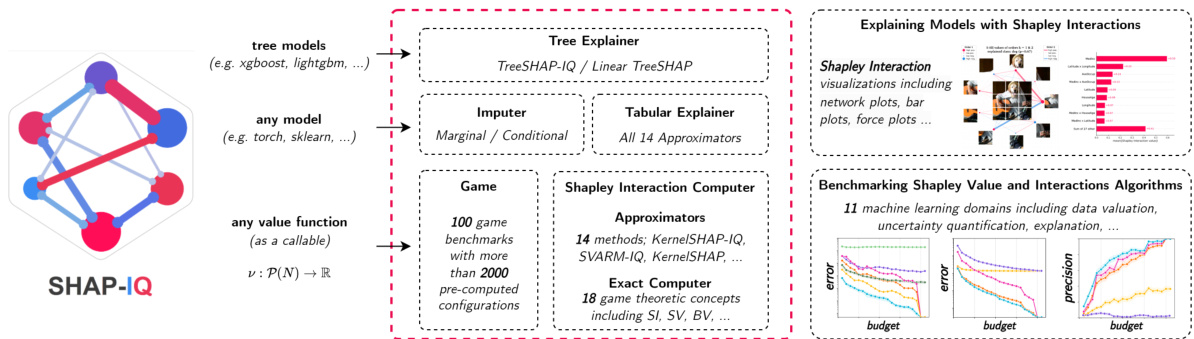
Figure 1: The shapiq Python package facilitates research on game theory for machine learning, including state-of-the-art approximation algorithms and pre-computed benchmarks. Moreover, it provides a simple interface for explaining predictions of machine learning models beyond feature attributions.
图 1: shapiq Python语言包促进了机器学习中博弈论的研究,包括最先进的近似算法和预计算的基准测试。此外,它还提供了一个简单的接口,用于解释机器学习模型的预测,超越了特征归因。
Shapley Interactions (SIs) [10, 33, 74, 77] distribute the overall worth to all groups of entities up to a maximum explanation order. They satisfy axioms similar to the SV, to which they reduce for individuals, i.e. the lowest explanation order. In contrast, for the highest explanation order, which comprises an interaction for every coalition, the SIs yield the Möbius Interaction (MI), or Möbius transform [27, 35, 69]. The MIs are a fundamental concept in cooperative game theory that captures the isolated joint contribution, which allows to additively describe every coalition’s worth by a sum of the contained MIs. With an increasing explanation order, the SIs comprise more components that finally yield the MIs as the most comprehensive explanation of the game at the cost of highest complexity [10, 77]. While the SV and SIs provide an appealing theoretical concept, computing them without structural assumptions on the game requires exponential complexity [22]. For tree-based models, it was shown that SVs [51, 83] and SIs [58, 84] can be efficiently computed by exploiting the architecture. Moreover, game-agnostic stochastic ap proxima tors estimate the SV [11, 17, 43, 52, 54, 61, 65] and SIs [28, 29, 44, 74, 77] with a limited budget of game evaluations.
Shapley交互 (SIs) [10, 33, 74, 77] 将整体价值分配给所有实体组,最多达到最大解释阶数。它们满足与SV类似的公理,对于个体而言,它们简化为SV,即最低解释阶数。相反,对于最高解释阶数,包含每个联盟的交互,SIs产生Möbius交互 (MI) 或Möbius变换 [27, 35, 69]。MI是合作博弈论中的一个基本概念,它捕捉了孤立的联合贡献,允许通过包含的MI的加和来描述每个联盟的价值。随着解释阶数的增加,SIs包含更多组件,最终产生MI作为对游戏的最全面解释,但代价是最高复杂度 [10, 77]。虽然SV和SIs提供了吸引人的理论概念,但如果没有对游戏的结构假设,计算它们需要指数级复杂度 [22]。对于基于树的模型,已经证明可以通过利用架构高效计算SVs [51, 83] 和 SIs [58, 84]。此外,与游戏无关的随机近似器在有限的游戏评估预算下估计SV [11, 17, 43, 52, 54, 61, 65] 和 SIs [28, 29, 44, 74, 77]。
Diverse applications of the SV have led to various techniques for its efficient computation [13]. Recently, extensions to any-order SIs addressed limitations of the SV and complemented interpretation of model predictions with higher-order feature interactions [10, 29, 74, 77, 78]. While stochastic ap proxima tors are applicable to any game, their evaluation is typically performed in an isolated application [29, 47], such as feature interactions. Moreover, implementing such algorithms requires a strong mathematical background and specific design choices. Existing Python packages, such as shap [52], provide a relatively small number of ap proxima tors, which are limited to the SV and feature attributions.
SV的多样化应用导致了其高效计算的各种技术[13]。最近,扩展到任意阶的 SIs 解决了 SV 的局限性,并通过高阶特征交互补充了模型预测的解释[10, 29, 74, 77, 78]。虽然随机逼近器适用于任何游戏,但其评估通常在孤立的应用程序中进行[29, 47],例如特征交互。此外,实现此类算法需要较强的数学背景和特定的设计选择。现有的 Python语言 包,如 shap [52],提供了相对较少的逼近器,这些逼近器仅限于 SV 和特征归因。
Contribution. In this work, keeping within the scope of the NeurIPS 2024 Datasets & Benchmark track, we present shapiq, an open-source Python library for any-order SIs that consolidates research for computing SVs and SIs across ML domains. Therein, we contribute
贡献。在本工作中,我们围绕 NeurIPS 2024 数据集与基准赛道的主题,推出了 shapiq,一个开源的 Python语言库,用于计算任意阶的 SIs(Shapley Interaction Indices),并整合了跨机器学习领域计算 SVs(Shapley Values)和 SIs 的研究成果。在此过程中,我们做出了以下贡献:
Related software tools and benchmarks. shapiq extends the popular shap [52] Python package beyond feature attributions aiming to fully embrace the application of SVs and SIs in ML. While shap implements a single index for 2-order feature interactions to explain the predictions of tree-based models, shapiq implements a dozen ap proxima tors for any-order SIs and offers a benchmarking suite for these algorithms across 10 different domains (Table 2). Related software such as aix360 [4], alibi [40] and dalex [6] are general toolboxes offering the implementation and visualization of the most popular ML explanations for end-users. We specify in SIs to provide a comprehensive tool facilitating research in game theory for ML, including the exact computation of 18 interaction indices and game-theoretic concepts (Table 1). Notably, the inn vest i gate [3] and captum [42] Python packages offer feature attribution explanation methods specific to (deep) neural networks. Most recently, quantus [36] implements evaluation metrics for these explanation methods.
相关软件工具与基准。shapiq 扩展了广受欢迎的 shap [52] Python 包,超越了特征归因,旨在全面支持 SVs 和 SIs 在机器学习中的应用。尽管 shap 仅实现了 2 阶特征交互的单一索引来解释基于树模型的预测,shapiq 则实现了适用于任意阶 SIs 的多种近似算法,并提供了这些算法在 10 个不同领域的基准测试套件(表 2)。相关软件如 aix360 [4]、alibi [40] 和 dalex [6] 是通用工具箱,为终端用户提供最流行的机器学习解释方法及其可视化。我们在 SIs 中专门提供了一个全面工具,以促进机器学习中的博弈论研究,包括 18 种交互指数和博弈论概念的精确计算(表 1)。值得注意的是,innvestigate [3] 和 captum [42] Python 包提供了专门针对(深度)神经网络的特征归因解释方法。最近,quantus [36] 实现了这些解释方法的评估指标。
Table 1: Available concepts in the Exact Computer class in shapiq with SIs in bold.
表 1: shapiq 中 Exact Computer 类别的可用概念,其中 SI 以粗体显示。
| Setting | Interaction Index (I1) [27] | BaseSemivalue[23] | GeneralizedValue(GV)[55] |
|---|---|---|---|
| Machine Learning | k-Shapley Values (k-SIH) [10] Shapley Taylor II (STII) [74] Faithful Shapley II (FSIM) [77] kADD-SHAP[65] Faithful Banzhaf II (FBII)[77] | Shapley(SV)[72] Banzhaf (BV) [8] | Joint SV [34] |
| Game Theory | Mobius(M1)[27,35,69] Co-Mobius (Co-MI) [32] Shapley II (SIM) [33] Chaining ⅡI (CHII) [57] BanzhafII(BII)[33] | Shapley (SV) [72] Banzhaf(BV)[8] | InternalGV(IGV)[55] ExternalGV(EGV)[55] ShapleyGV(SGV)[56] Chaining GV (CHGV) [55] BanzhafGV(BGV)[57] |
We build upon recent advances in benchmarking explain able artificial intelligence (XAI) methods such as feature attributions [2, 48, 50, 60] and algorithms for data valuation [37]. XAI-Bench [50] focuses on synthetic tabular data. OpenXAI [2] provides 7 real-world tabular datasets with pre-trained neural network models, 7 feature attribution methods and 8 metrics to compare them. $\mathcal{M}^{4}$ [48] extends OpenXAI to benchmark feature attributions of deep neural networks for image and text modalities. In [60], the authors benchmark several algorithms for approximating SVs based on the conditional feature distribution. Open Data Val [37] provides 9 real-world datasets, 11 data valuation methods and 4 metrics to compare them. shapiq puts more focus on benchmarking higher-order SI algorithms and provides an interface to state-of-the-art explanation methods that base on SIs, e.g. TreeSHAP-IQ [58]. While open data repositories such as OpenML [9] offer easy access to datasets for ML, we pre-compute and share ground-truth SIs for various games (i.e. dataset–model pairs) that saves considerate time and resources when benchmarking approximation algorithms.
我们基于近期在可解释人工智能 (XAI) 方法基准测试方面的进展,例如特征归因 [2, 48, 50, 60] 和数据估值算法 [37]。XAI-Bench [50] 专注于合成的表格数据。OpenXAI [2] 提供了 7 个真实世界的表格数据集、预训练的神经网络模型、7 种特征归因方法和 8 个用于比较的指标。$\mathcal{M}^{4}$ [48] 扩展了 OpenXAI,以基准测试深度神经网络在图像和文本模态中的特征归因。在 [60] 中,作者基于条件特征分布对几种近似 Shapley 值 (SVs) 的算法进行了基准测试。Open Data Val [37] 提供了 9 个真实世界的数据集、11 种数据估值方法和 4 个用于比较的指标。shapiq 更加侧重于高阶 Shapley 交互指数 (SI) 算法的基准测试,并提供了一个基于 SI 的最新解释方法的接口,例如 TreeSHAP-IQ [58]。虽然像 OpenML [9] 这样的开放数据仓库可以方便地访问机器学习数据集,但我们预先计算并分享了各种游戏(即数据集-模型对)的真实 SI,这为基准测试近似算法节省了大量时间和资源。
2 Theoretical Background
2 理论背景
In ML, various concepts are based on synergies of entities to optimize performance in a given task. For example, weak learners construct powerful model ensembles [70], collected data instances and features are used to train supervised ML models [16, 30], where feature values collectively predict outputs. To better understand such processes, XAI quantifies the contributions of these entities to the task, most prominently for feature values in predictions (local feature attribution [52, 73]), features in models (global feature importance [16, 17, 66]), and data instances in model training (data valuation [30]). Assigning such contributions is closely related to the field of cooperative game theory [71], which studies the notion of value for players that collectively obtain a payout. To adequately assess the impact of individual players, it is necessary to analyze the payout for different coalitions. More formally, a cooperative game $\nu:\mathcal{P}(N)\to\mathbb{R}$ with $\nu({\dot{\emptyset}})=0$ is defined by a value function on the power set of $N:={1,\dots,n}$ entities, which describes such payouts for all possible coalitions of players. We later summarize such prominent examples in the context of ML in Table 3. Here, we summarize existing contribution concepts for individuals and groups of entities, outlined in Table 1.
在机器学习中,各种概念基于实体的协同作用,以优化给定任务中的性能。例如,弱学习器构建强大的模型集成 [70],收集的数据实例和特征用于训练监督机器学习模型 [16, 30],其中特征值共同预测输出。为了更好地理解这些过程,可解释人工智能 (XAI) 量化了这些实体对任务的贡献,最显著的是预测中的特征值(局部特征归因 [52, 73])、模型中的特征(全局特征重要性 [16, 17, 66])以及模型训练中的数据实例(数据估值 [30])。分配这些贡献与协作博弈论 [71] 密切相关,该理论研究共同获得回报的玩家的价值概念。为了充分评估个体玩家的影响,有必要分析不同联盟的回报。更正式地说,协作博弈 $\nu:\mathcal{P}(N)\to\mathbb{R}$ 与 $\nu({\dot{\emptyset}})=0$ 由 $N:={1,\dots,n}$ 实体的幂集上的值函数定义,该函数描述了所有可能玩家联盟的回报。我们稍后在表 3 中总结了机器学习背景下的这些显著例子。在此,我们总结了表 1 中概述的个体和实体群体的现有贡献概念。
The SV [72] and Banzhaf Value (BV) [8] are instances of semivalues [23]. Semivalues assign contributions to individual players and adhere to intuitive axioms: Linearity enforces linearly composed contributions for linearly composed games; Dummy requires that players without impact receive zero contribution; Symmetry enforces that entities contributing equally to the payout receive equal value. The SV [72] is the unique semivalue that additionally satisfies efficiency, i.e. the sum of all contributions yields the total payout $\nu(N)$ . In contrast, the BV [8] is the unique semivalue that additionally satisfies 2-Efficiency, i.e. the contributions of two players sum to the contribution of a joint player in a reduced game, where both players are merged. The SV and BV are represented as a weighted average over marginal contributions $\Delta_{i}(T):=\nu(T\cup{i})-\nu(T)$ for $i\in N$ as
SV [72] 和 Banzhaf 值 (BV) [8] 是半值 (semivalues) [23] 的实例。半值为个体玩家分配贡献,并遵循直观的公理:线性性要求线性组合的游戏贡献也是线性组合的;虚拟玩家要求没有影响的玩家贡献为零;对称性要求对收益贡献相等的实体获得相等的价值。SV [72] 是唯一满足效率性的半值,即所有贡献的总和等于总收益 $\nu(N)$。相比之下,BV [8] 是唯一满足 2-效率性的半值,即两个玩家的贡献之和等于在简化游戏中合并后的联合玩家的贡献。SV 和 BV 表示为边际贡献 $\Delta_{i}(T):=\nu(T\cup{i})-\nu(T)$ 的加权平均值,其中 $i\in N$。

In ML applications, the SV is typically preferred over the BV due to the efficiency axiom [71]. For instance, in local feature attribution, the SV is utilized to fairly distribute the model’s prediction to individual features [52, 73]. However, it was shown that the SV is limited when explaining complex decision systems, and feature interactions, i.e. the joint contributions of features’ groups, are required to understand such processes [20, 29, 45, 46, 58, 63, 74, 77, 78, 82].
在机器学习应用中,由于效率公理 [71],SV 通常比 BV 更受青睐。例如,在局部特征归因中,SV 被用于公平地将模型的预测分配给各个特征 [52, 73]。然而,研究表明,在解释复杂决策系统时,SV 存在局限性,理解这些过程需要特征交互,即特征组的联合贡献 [20, 29, 45, 46, 58, 63, 74, 77, 78, 82]。
The Generalized Value (GV) [55] and Interaction Index $(\mathbf{II})$ [27] are two paradigms to extend the notion of value to groups of entities. The GVs are based on weighted averages over (joint) marginal contributions $\bar{\nu}(T\cup S)-\nu(T)$ for $S\subseteq N$ given $T\subseteq N\setminus{\bar{S}}$ . In contrast, IIs are based on discrete derivatives that account for lower-order effects of subsets of $S$ . For instance, for two players $i,j\in N$ , the discrete derivative $\Delta_{{i,j}}(T)$ is defined as the joint marginal contribution $\nu(T\cup{i,j})-\nu(T)$ minus the individual marginal contributions $\Delta_{i}(T)$ and $\Delta_{j}(T)$ . More generally, the discrete derivative $\Delta_{S}(T)$ for $S\subseteq N$ in the presence of $T\subseteq N\setminus S$ is defined as
广义价值 (Generalized Value, GV) [55] 和交互指数 (Interaction Index, II) [27] 是将价值概念扩展到实体群体的两种范式。广义价值基于对联合边际贡献 $\bar{\nu}(T\cup S)-\nu(T)$ 的加权平均,其中 $S\subseteq N$ 且给定 $T\subseteq N\setminus{\bar{S}}$。相比之下,交互指数基于离散导数,这些导数考虑了 $S$ 子集的低阶效应。例如,对于两个玩家 $i,j\in N$,离散导数 $\Delta_{{i,j}}(T)$ 被定义为联合边际贡献 $\nu(T\cup{i,j})-\nu(T)$ 减去个体边际贡献 $\Delta_{i}(T)$ 和 $\Delta_{j}(T)$。更一般地,对于 $S\subseteq N$ 在 $T\subseteq N\setminus S$ 存在的情况下,离散导数 $\Delta_{S}(T)$ 被定义为

A positive value indicates synergy, whereas a negative value indicates redundancy of $S$ given $T$ . Lastly, a zero value indicates (additive) independence, i.e. the joint marginal contribution is equal to the sum of all lower-order effects. GVs and IIs are uniquely represented [27, 55] by
正值表示协同效应,负值表示在给定 $T$ 的情况下 $S$ 的冗余。最后,零值表示(加性)独立性,即联合边际贡献等于所有低阶效应的总和。GVs 和 IIs 是唯一表示的 [27, 55]。

The most prominent examples are the Shapley $G V\left(S G V\right)$ [56] and the Shapley $I I$ (SII) [33] with $p_{t}^{s}(n)=\bar{\left((n-s+1)\binom{n-s}{t}\right)}^{-1}$ , which naturally extend the SV (cf. Appendix A.1). While the SGV and SII are natural extensions to the SV, they are not suitable for interpret ability, since they are defined on the powerset and comprise an exponential number of components. Moreover, neither GVs nor IIs satisfy the efficiency axiom for higher-orders, which is desirable for ML applications.
最典型的例子是 Shapley $G V\left(S G V\right)$ [56] 和 Shapley $I I$ (SII) [33],其中 $p_{t}^{s}(n)=\bar{\left((n-s+1)\binom{n-s}{t}\right)}^{-1}$,它们自然地扩展了 SV(参见附录 A.1)。虽然 SGV 和 SII 是 SV 的自然扩展,但由于它们定义在幂集上并且包含指数级数量的组件,因此不适合用于可解释性。此外,GVs 和 IIs 都不满足高阶的效率公理,而这对于机器学习应用是必要的。
Shapley Interactions (SIs) for Machine Learning assign joint contribution $\Phi_{k}$ up to an explanation order $k$ , i.e. for all coalitions $S\subseteq N$ with $|S|\le k$ , which satisfy generalized efficiency $\nu(N)=$ $\begin{array}{r}{\sum_{S\subseteq N,|S|\leq k}\Phi_{k}(S).}\end{array}$ . The $k{\mathrm{-}}S V s$ ( $k$ -SIIs) [10] are the unique SIs that coincide with SII for the highest order. The Shapley Taylor $I I$ (STII) [74] puts a stronger emphasis on the top-order interactions, and Faithful SII (FSII) [77] optimizes Shapley-weighted faithfulness
机器学习中的Shapley交互作用(SIs)分配的联合贡献 $\Phi_{k}$ 最高到解释阶数 $k$ ,即对于所有满足广义效率 $\nu(N)=$ $\begin{array}{r}{\sum_{S\subseteq N,|S|\leq k}\Phi_{k}(S).}\end{array}$ 的联盟 $S\subseteq N$ 且 $|S|\le k$ 。 $k{\mathrm{-}}S V s$ ( $k$ -SIIs) [10] 是唯一的SIs,它们与最高阶的SII一致。Shapley Taylor $I I$ (STII) [74] 更加强调高阶交互作用,而Faithful SII (FSII) [77] 优化了Shapley加权的忠实性

FSII is thus $\begin{array}{r}{\Phi_{k}^{\mathrm{FSII}}:=\arg\operatorname*{min}{\Phi{k}}\mathcal{L}(\boldsymbol{\nu},\Phi_{k})}\end{array}$ , where $\mu_{\infty}\gg1$ ensures efficiency. It was recently shown that pairwise SII and consequently $k$ -SII with $k=2$ optimize a faithfulness metric with slightly different weights [28]. For $k=1$ , all SIs reduce to the SV $\Phi_{1}\equiv\phi^{\mathrm{{SV}}}$ , which minimizes faithfulness $\mathcal{L}(\nu,\Phi_{1})$ [12] with the efficiency constraint, or equivalently $\mu_{\infty}\to\infty$ [28, 52]. Finally, for $k=n$ , all SIs $\Phi_{n}$ are the $M I s$ (cf. Appendix A.2), which are faithful to all game values, i.e. $\mathcal{L}(\nu,\Phi_{n})=0$ . Notably, all SIs can be uniquely represented by the MIs [31]. In this context, SIs yield a complexity-accuracy trade-off, ranging from the least complex (SV) to the most comprehensive (MI) explanation. Other extensions include $k_{A D D}–S H A P$ [65] of the SV and Faithful BII (FBII) [77] of the BV, which do not satisfy efficiency, as well as Joint $S V s$ [34], a GV with efficiency. However, in the context of feature interactions and ML, SIs are preferred over GV-based (Joint SVs) or BV-based IIs (FBII), as they account for lower-order interactions and adhere to the SV and MI as edge cases.
因此,FSII为 $\begin{array}{r}{\Phi_{k}^{\mathrm{FSII}}:=\arg\operatorname*{min}{\Phi{k}}\mathcal{L}(\boldsymbol{\nu},\Phi_{k})}\end{array}$,其中 $\mu_{\infty}\gg1$ 确保效率。最近研究表明,成对 SII 以及 $k=2$ 时的 $k$-SII 优化了具有略微不同权重的忠实度度量 [28]。对于 $k=1$,所有 SI 都简化为 SV $\Phi_{1}\equiv\phi^{\mathrm{{SV}}}$,它在效率约束下最小化忠实度 $\mathcal{L}(\nu,\Phi_{1})$ [12],或者等价于 $\mu_{\infty}\to\infty$ [28, 52]。最后,对于 $k=n$,所有 SI $\Phi_{n}$ 都是 MI(参见附录 A.2),它们对所有博弈值都忠实,即 $\mathcal{L}(\nu,\Phi_{n})=0$。值得注意的是,所有 SI 都可以通过 MI 唯一表示 [31]。在这种情况下,SI 产生了复杂度-准确性的权衡,从最不复杂(SV)到最全面(MI)的解释。其他扩展包括不满足效率的 SV 的 $k_{A D D}–S H A P$ [65] 和 BV 的忠实 BII (FBII) [77],以及具有效率的 GV 联合 SV [34]。然而,在特征交互和机器学习的背景下,SI 优于基于 GV(联合 SV)或基于 BV 的 II(FBII),因为它们考虑了低阶交互并遵循 SV 和 MI 作为边缘情况。
3 Overview of the shapiq Python package
3 shapiq Python语言包概述
The shapiq package accelerates research on SIs for ML, and provides a simple interface for explaining any-order feature interactions in predictions of ML models. Its code is open-source on GitHub at https://github.com/mmschlk while the documentation with notebook examples and API reference is available at https://shapiq.read the docs.io.
shapiq 包加速了机器学习中特征交互重要性 (SIs) 的研究,并提供了一个简单的接口,用于解释机器学习模型预测中的任意阶特征交互。其代码在 GitHub 上开源,地址为 https://github.com/mmschlk,而包含笔记本示例和 API 参考的文档可在 https://shapiq.readthedocs.io 上查阅。
Table 2: Overview of methods in shapiq and applicable SIs. Explainers rely on ap proxima tors or model assumptions. $(\checkmark)$ indicates only top-order approximation.
表 2: shapiq 中方法的概述及适用的 SIs。解释器依赖于近似器或模型假设。$(\checkmark)$ 表示仅支持高阶近似。
| 类别 | 实现 | 来源 | SV | (k-)SII | STII | FSII |
|---|---|---|---|---|---|---|
| 近似器 | SHAP-IQ | [29] | (S) | |||
| 近似器 | SVARM-IQ | [44] | < | (<) | ||
| 近似器 | Permutation Sampling (SIH) | [77] | 一 | |||
| 近似器 | Permutation Sampling (STII) | [74] | 一 | 一 | ||
| 近似器 | KernelSHAP-IQ | [28] | 一 | 一 | ||
| 近似器 | Inconsistent KernelSHAP-IQ | [28] | ||||
| 近似器 | FSII Regression | [77] | 一 | ← | ||
| 近似器 | KernelSHAP | [52] | 一 | |||
| 近似器 | KADD-SHAP | [65] | 一 | |||
| 近似器 | Unbiased KernelSHAP | [17] | 一 | 一 | ||
| 近似器 | SVARM | [43] | 一 | |||
| 近似器 | Permutation Sampling | [11] | 一 | 一 | ||
| 近似器 | Owen Sampling | [61] | 一 | 一 | ||
| 近似器 | Stratified Sampling | [54] | 一 | 一 | ||
| 解释器 | Agnostic (Marginal) | - | √ | √ | ||
| 解释器 | Agnostic (Conditional) | |||||
| 解释器 | TreeSHAP-IQ | [58] | (S) | |||
| 解释器 | Linear TreeSHAP | [51, 83] | 一 | |||
| 计算器 | Mobius Converter | √ | √ | |||
| 计算器 | Exact Computer |
3.1 shapiq Facilitates Research on Shapley Interactions for Machine Learning
3.1 shapiq 促进机器学习 Shapley 交互作用的研究
Ap proxima tors. We implement 7 algorithms for approximating SIs across 4 different interaction indices, and another 7 algorithms for approximating SVs. Table 2 provides a comprehensive overview of this effort, where the shapiq.Approx im at or class is extended with each implementation. We unify common approximation methods by including a general shapiq.Coalition Sampler interface offering approximation performance increases through sampling procedures like the border- and pairing-tricks introduced in [17, 29]. Algorithms are primarily benchmarked based on how well they approximate the ground truth SIs values that often cannot be computed in practice due to exponential complexity and constrained resources.
近似器。我们实现了7种算法来近似4种不同的交互指数(SIs),以及另外7种算法来近似Shapley值(SVs)。表2提供了这一工作的全面概述,其中shapiq.Approximator类通过每个实现进行了扩展。我们通过引入通用的shapiq.CoalitionSampler接口统一了常见的近似方法,该接口通过诸如[17, 29]中引入的边界和配对技巧等采样程序提高了近似性能。算法主要基于它们如何近似真实SIs值进行基准测试,这些值通常由于指数复杂性和资源限制而无法在实践中计算。
Exact computer. A key functionality of shapiq lies in computing the SIs exactly, which is feasible for smaller games, but reaches its limit for growing player numbers. The shapiq.Exact Computer class provides an interface for computing 18 interaction indices and game-theoretic concepts, including the MIs (see Table 1).
精确计算器。shapiq 的一个关键功能在于精确计算交互指数(SIs),这对于较小的博弈是可行的,但随着玩家数量的增加,其计算能力会达到极限。shapiq.Exact Computer 类提供了一个接口,用于计算 18 种交互指数和博弈论概念,包括 MIs(见表 1)。
Games. Ap proxima tors and computers work given a specified cooperative game. Table 3 describes in detail 11 benchmark games implemented in shapiq. Beyond synthetic games, our benchmark spans the 5 most prominent domains where SIs can be applied for ML. The shapiq.Game class can be easily extended to include future benchmarks in the package. We pre-compute and share exact SIs for 2 042 benchmark game configurations in total (Appendix B), facilitating future work on improving the ap proxima tors, which we elaborate on further in Section 4.
游戏。近似器和计算机在给定指定的合作游戏中工作。表 3 详细描述了在 shapiq 中实现的 11 个基准游戏。除了合成游戏外,我们的基准涵盖了 SI 可以应用于机器学习的 5 个最突出的领域。shapiq.Game 类可以轻松扩展以包含未来的基准。我们预先计算并共享了总共 2042 个基准游戏配置的精确 SI(附录 B),为未来改进近似器的工作提供了便利,我们将在第 4 节中进一步详细阐述。
3.2 Explaining Machine Learning Predictions with shapiq
3.2 使用shapiq解释机器学习预测
Explainer. The shapiq.Explainer class is a simplified interface to explain any-order feature interactions in ML models. Figure 2 goes through exemplary code used to approximate SIs for a single prediction and visualize them on a graph plot. Currently two classes are further distinguished within the API, but we envision extending shapiq.Explainer to include more data modalities and model algorithms. shapiq.Tabular Explain er allows for model-agnostic explanation based on feature margin aliz ation with either marginal or conditional imputation (refer to Appendix C for details). shapiq.Tree Explain er implements TreeSHAP-IQ [58] for efficient explanations specific to decision tree-based models, e.g. random forest or gradient boosting decision trees, with native support for scikit-learn [64], xgboost [15], and lightgbm [38]. Figure 3 goes through
Explainer。shapiq.Explainer 类是一个简化的接口,用于解释机器学习模型中的任意顺序特征交互。图 2 展示了用于近似单个预测的 SIs 并在图表上可视化的示例代码。目前,API 中进一步区分了两类,但我们计划扩展 shapiq.Explainer 以包含更多数据模式和模型算法。shapiq.TabularExplainer 允许基于特征边际化的模型无关解释,支持边际或条件插补(详见附录 C)。shapiq.TreeExplainer 实现了 TreeSHAP-IQ [58],用于特定于基于决策树的模型(如随机森林或梯度提升决策树)的高效解释,并原生支持 scikit-learn [64]、xgboost [15] 和 lightgbm [38]。图 3 展示了
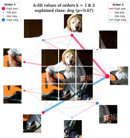
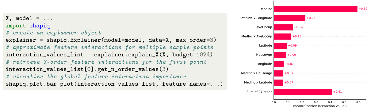
Figure 2: Left: Exemplary code for locally explaining a single model’s prediction with shapiq. Right: Local feature interactions visualized on a network plot.
图 2: 左:使用 shapiq 对单个模型预测进行本地解释的示例代码。右:在网络图中可视化的本地特征交互。
Figure 3: Left: Exemplary code for globally explaining multiple model’s predictions with shapiq. Right: Global feature interaction importance visualized as a bar plot.
图 3: 左:使用 shapiq 全局解释多个模型预测的示例代码。右:全局特征交互重要性以条形图形式可视化。
exemplary code for explaining a set of predictions and visualizing their aggregation in a bar plot, which represents the global feature interaction importance.
用于解释一组预测并在柱状图中可视化其聚合的示例代码,该图表示全局特征交互重要性。
Utility functions. shapiq offers additional useful tools that are described in detail in the documentation. Interaction values are stored and processed using the shapiq.Interaction Values data class, which is rich in utility functions. The shapiq.plot module supports the visualization of interaction values, including our custom network plot, but also wrapping the well-known force and bar plots from shap [52]. Finally, shapiq.datasets loads datasets used for testing and examples.
实用函数。shapiq 提供了额外的实用工具,详细内容在文档中有描述。交互值使用 shapiq.Interaction Values 数据类进行存储和处理,该类包含丰富的实用函数。shapiq.plot 模块支持交互值的可视化,包括我们自定义的网络图,同时也封装了 shap [52] 中知名的力导向图和条形图。最后,shapiq.datasets 加载用于测试和示例的数据集。
4 Benchmarking Analysis
4 基准分析
The shapiq library enables computation of various SIs for a broad class of application domains. To illustrate its versatility, we conduct benchmarks across a wide variety of traditional ML-based SV application scenarios. The ML benchmark demonstrates how higher-order SIs enable an accuracy– complexity trade-off for model interpret ability (Section 4.1) and highlights that different approximation techniques in shapiq achieve the state-of-the-art performance depending on the application domains (Section 4.2). Tables 3, 4 and 5 present an overview of different application domains and associated benchmarks. Depending on the benchmark, it can be instantiated with different datasets, models, player numbers or benchmark-specific configuration parameters, e.g. uncertainty type: epistemic for Uncertainty Explanation or imputer: conditional for Local Explanation. In total, shapiq offers 100 unique benchmark games, i.e. applications times dataset–model pairs.
shapiq 库支持在广泛的应用领域中计算各种 SIs。为了展示其多功能性,我们在各种传统的基于机器学习的 SV 应用场景中进行了基准测试。机器学习基准测试展示了高阶 SIs 如何实现模型可解释性的准确性与复杂性之间的权衡(第 4.1 节),并强调了 shapiq 中不同的近似技术在不同应用领域中实现了最先进的性能(第 4.2 节)。表 3、表 4 和表 5 概述了不同的应用领域及相关基准测试。根据基准测试的不同,可以使用不同的数据集、模型、玩家数量或特定于基准测试的配置参数进行实例化,例如不确定性类型:用于不确定性解释的认知不确定性或插值器:用于局部解释的条件插值器。shapiq 总共提供了 100 个独特的基准测试游戏,即应用与数据集-模型对的组合。
For all games that include $n\leq16$ players, the value functions have been pre-computed by evaluating all coalitions and storing the games to file. Reading a pre-computed game from file, instead of performing up to $2^{16}=\bar{6}553\bar{6}$ value function calls with each new experiment run, saves valuable computational time and contributes to reproducibility as well as sustainability. This is particularly beneficial for tasks that involve remove-and-refit strategies [19], such as Data Valuation or Feature Selection. For $n>16$ , where pre-computing a game and ground truth values becomes computationally prohibitive, we rely on analytical solutions to compute the ground truth like TreeSHAP-IQ [58] for tree-based ensembles or the MI representation of Sum of Unanimity Models [28, 29, 77]. For details regarding the experimental setting and reproducibility, we refer to Appendix D.
对于所有包含 $n\leq16$ 名玩家的游戏,值函数已通过评估所有联盟并将游戏存储到文件中进行了预计算。从文件中读取预计算的游戏,而不是在每次新实验运行时进行最多 $2^{16}=\bar{6}553\bar{6}$ 次值函数调用,节省了宝贵的计算时间,并有助于提高可重复性和可持续性。这对于涉及移除和重新拟合策略 [19] 的任务(如数据估值或特征选择)尤其有益。对于 $n>16$ 的情况,由于预计算游戏和真实值在计算上变得不可行,我们依靠分析解决方案来计算真实值,例如用于基于树的集成的 TreeSHAP-IQ [58],或一致模型和的 MI 表示 [28, 29, 77]。有关实验设置和可重复性的详细信息,请参阅附录 D。
Table 3: Overview of the available benchmark games and domains in shapiq. Each benchmark can be instantiated with different datasets, models, player sizes, or benchmark-specific configuration parameters. This results in 2 042 pre-computed individual configurations (see Tables 4 and 5) .
表 3: shapiq 中可用的基准游戏和领域概览。每个基准都可以使用不同的数据集、模型、玩家规模或特定于基准的配置参数进行实例化。这导致了 2 042 个预先计算的单独配置(见表 4 和表 5)。
| 领域 | 基准(游戏) | 来源 | 玩家 | 联盟价值 |
|---|---|---|---|---|
| XAI | 局部解释 | [52,73] | 特征 | 模型输出 |
| 全局解释 | [18] | 特征 | 模型损失 | |
| 树解释 | [51,58] | 特征 | 模型输出 | |
| 不确定性 | 不确定性解释 | [80] | 特征 | 预测熵 |
| 模型选择 | 特征选择 | [16, 66] | 特征 | 性能 |
| 集成选择 | [70] | 弱学习器 | 性能 | |
| 估值 | RF 集成选择 | [70] | 树模型 | 性能 |
| 数据估值 | [30] | 数据点 | 性能 | |
| 数据集估值 | [76] | 数据子集 | 性能 | |
| 无监督学习 | 聚类解释 | 特征 | 聚类分数 | |
| 无监督特征重要性 | [5] | 特征 | 总相关性 | |
| 合成 | 一致性模型求和 | [28,77] | 玩家 | 一致投票求和 |
4.1 Accuracy – Complexity Trade-Off of Shapley Interactions for Interpret ability
4.1 解释性中Shapley交互的准确性与复杂性权衡
In this experiment, we empirically evaluate faithfulness of SIs for varying explanation orders $k$ . To this end, we rely on the Shapley-weighted faithfulness $\mathcal{L}(\nu,\Phi_{k})$ introduced in Section 2. SIs range from the SV (least complex) to the MI (most complex) explanation, where the SV minimizes $\mathcal{L}(\bar{\nu},\Phi_{1})$ for $k=1$ [12, 52], and MIs are faithful to all game values with $\mathcal{L}(\nu,\Phi_{n})=0$ for $k=n$ [10, 77]. Figure 4 shows the Shapley-weighted $R^{2}$ value for $k=1,\hdots,n$ for a synthetic game with a single interaction of varying size (a) and real-world ML applications (b). Here, we used $\mu_{\infty}=1$ instead of $\mu_{\infty}\gg1$ , which affects FBII that violates efficiency. The results show that in general SIs become more faithful with higher explanation order. Notably, the difference between pairwise SIs and SVs (SHAP textbox) is remarkable, where pairwise interactions $(k=2)$ ) already yield a strong improvement in faithfulness. If higher-order interactions dominate, then SIs require a larger explanation order to maintain faithfulness. While FSII and FBII are optimized for faithfulness, STII and $k$ -SII do not necessarily yield a strict improvement in this metric. In fact, it was shown that SII and $k$ -SII optimize a slightly different faithfulness metric, which changes for every order [28]. Yet, we observe a consistent strong improvement of pairwise $k$ -SII over the SV (SHAP). While FSII and FBII optimize faithfulness, $k$ -SII and STII adhere to strict structural assumptions, where STII projects all higher-order interactions to the top-order SIs, and $k$ -SII is consistent with SII. Pra citi on ers may choose SIs tailored to their specific application, where $k$ -SII is a good default choice for shapiq.
在本实验中,我们实证评估了在不同解释顺序 $k$ 下的 SIs 的忠实性。为此,我们依赖于第 2 节中介绍的 Shapley加权忠实性 $\mathcal{L}(\nu,\Phi_{k})$。SIs 从 SV(最不复杂)到 MI(最复杂)的解释范围,其中 SV 在 $k=1$ 时最小化 $\mathcal{L}(\bar{\nu},\Phi_{1})$ [12, 52],而 MIs 对所有游戏值忠实,当 $k=n$ 时,$\mathcal{L}(\nu,\Phi_{n})=0$ [10, 77]。图 4 展示了 Shapley加权的 $R^{2}$ 值,针对 $k=1,\hdots,n$ 的情况,分别对应一个具有不同大小单一交互的合成游戏(a)和实际机器学习应用(b)。在这里,我们使用了 $\mu_{\infty}=1$ 而不是 $\mu_{\infty}\gg1$,这影响了违反效率的 FBII。结果表明,通常随着解释顺序的增加,SIs 的忠实性也会提高。值得注意的是,成对 SIs 和 SVs(SHAP 文本框)之间的差异非常显著,其中成对交互 $(k=2)$ 已经在忠实性上带来了显著的提升。如果高阶交互占主导地位,那么 SIs 需要更大的解释顺序以保持忠实性。虽然 FSII 和 FBII 针对忠实性进行了优化,但 STII 和 $k$ -SII 并不一定在这一指标上带来严格的改进。事实上,研究表明 SII 和 $k$ -SII 优化了一个略微不同的忠实性指标,该指标随顺序变化 [28]。然而,我们观察到成对 $k$ -SII 相对于 SV(SHAP)的一致性强改进。虽然 FSII 和 FBII 优化了忠实性,但 $k$ -SII 和 STII 遵循严格的结构假设,其中 STII 将所有高阶交互投影到最高阶 SIs,而 $k$ -SII 与 SII 一致。实践者可以根据其具体应用选择定制的 SIs,其中 $k$ -SII 是 shapiq 的一个良好默认选择。
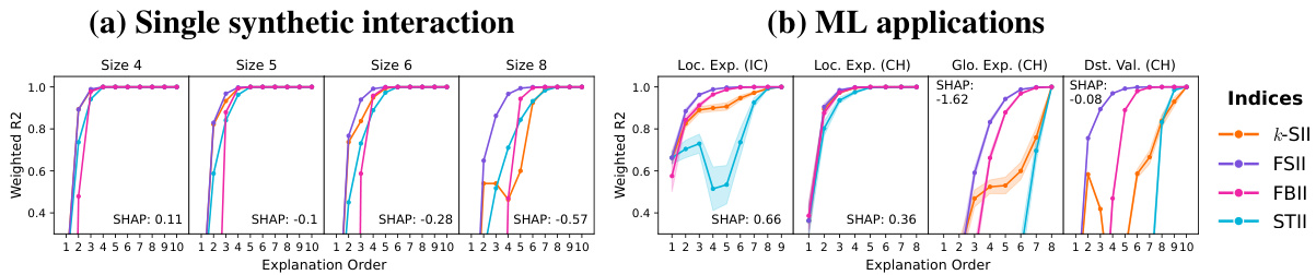
Figure 4: Shapley-weighted $R^{2}$ of interaction indices by explanation order for (a) single synthetic interactions and (b) ML applications. FSII is optimized for this metric, and increases faithfulness with each order. Interactions improve faithfulness over SHAP and yield an exact decomposition for the highest order. However, increasing interaction size negatively affects faithfulness.
图 4: (a) 单一合成交互和 (b) ML 应用中按解释顺序的交互指数的 Shapley 加权 $R^{2}$。FSII 针对该指标进行了优化,并随着顺序的增加提高了忠实度。交互比 SHAP 提高了忠实度,并为最高顺序提供了精确的分解。然而,增加交互规模会对忠实度产生负面影响。
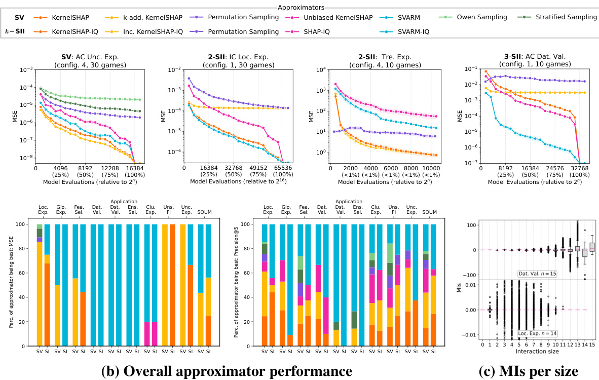
(a) Approximation quality in different application domains Figure 5: Overview of the benchmark results containing (a) budget-dependent MSE approximation curves on different benchmark settings, (b) a summary of the best performing ap proxima tors per setting over all 100 benchmark games measured by MSE (left) and Precision $\ @5$ (right), and (c) exemplary MIs for ten games of Data Valuation (top) and Local Explanation (bottom).
图 5: 基准测试结果概览,包含 (a) 不同基准设置下预算相关的 MSE 近似曲线,(b) 通过 MSE (左) 和 Precision $\ @5$ (右) 测量的所有 100 个基准游戏中每个设置下表现最佳的近似器汇总,以及 (c) 数据估值 (上) 和局部解释 (下) 十个游戏的示例 MI。
4.2 Comparison of Approximation Methods
4.2 近似方法比较
Various approximation methods for computing SIs are included in shapiq for a variety of SIs (cf. Table 2). The possibility of attributing (domain-specific) state-of-the-art performance to a single algorithm has been investigated empirically by multiple works [28, 29, 43, 44, 54, 61, 65, 77, 79]. We use the collection of 100 unique benchmark games in shapiq to evaluate the performance of different SV and SI approximation methods on a broad spectrum of ML applications. For each domain and configuration (see Table 4 and 5 in Appendix B), we compute ground truth SVs, 2-SIIs, and 3-SIIs and compare them with estimates provided by all ap proxima tors from Table 2. The ap proxima tors are run with a wide range of budget values and assessed by their achieved mean squared error (MSE) or precision at five (Precision $\ @5$ ). Figure 5 summarizes the approximation results.
shapiq 中包含了用于计算各种 SI 的多种近似方法(参见表 2)。多篇论文通过实证研究探讨了将(特定领域的)最先进性能归因于单一算法的可能性 [28, 29, 43, 44, 54, 61, 65, 77, 79]。我们使用 shapiq 中的 100 个独特基准游戏来评估不同 SV 和 SI 近似方法在广泛 ML 应用中的性能。对于每个领域和配置(参见附录 B 中的表 4 和表 5),我们计算了真实 SVs、2-SIIs 和 3-SIIs,并将它们与表 2 中所有近似方法提供的估计值进行比较。这些近似方法在广泛的预算值范围内运行,并通过其实现的均方误差 (MSE) 或五个精度 (Precision $\ @5$ ) 进行评估。图 5 总结了近似结果。
Most notably, the ranking of ap proxima tors varies strongly between the different applications domains, which is depicted in Figure 5 (a) and (b). This observation holds for both SVs and SIs. In general, two types of approximation methods dominate the application landscape in terms of MSE and Precision $\ @5$ . First, kernel-based approaches including KernelSHAP, $k_{\mathrm{ADD}}–\mathrm{SHAP}$ , KernelSHAP-IQ and Inconsistent KernelSHAP-IQ perform best for Local Explanation, Uncertainty Explanation, and Unsupervised Feature Importance. Second, the two stratification-based estimators SVARM and SVARM-IQ achieve state-of-the-art performance for Data Valuation, Dataset Valuation, or Ensemble Selection. Traditional mean-estimation methods including Permutation Sampling (SV and SII), Unbiased KernelSHAP, SHAPIQ, and Owen Sampling achieve moderate estimation qualities in comparison. Our findings give rise to the conclusion that stratification-based estimators perform superior in settings where the size of a coalition naturally impacts its worth (e.g. training size for Dataset Valuation), which is plausible as these methods group coalitions by size and thus leverage this dependency. Meanwhile, kernel-based estimators achieve state-of-the-art in settings where the dependency between size and worth of a coalition is less pronounced (e.g. sudden jumps of model predictions in Local Explanation).
最值得注意的是,近似方法的排名在不同应用领域之间存在显著差异,如图5(a)和(b)所示。这一观察适用于SVs和SIs。总体而言,就均方误差(MSE)和Precision@5而言,有两种类型的近似方法在应用场景中占据主导地位。首先,基于核的方法,包括KernelSHAP、$k_{\mathrm{ADD}}–\mathrm{SHAP}$、KernelSHAP-IQ和不一致的KernelSHAP-IQ,在局部解释、不确定性解释和无监督特征重要性方面表现最佳。其次,基于分层策略的估计器SVARM和SVARM-IQ在数据估值、数据集估值或集成选择方面实现了最先进的性能。相比之下,传统的均值估计方法,包括置换采样(SV和SII)、无偏KernelSHAP、SHAPIQ和Owen采样,则表现出中等水平的估计质量。我们的研究结果表明,在联盟规模自然影响其价值的场景中(例如数据集估值的训练规模),基于分层策略的估计器表现更优,这很合理,因为这些方法按规模对联盟进行分组,从而利用了这种依赖关系。与此同时,在联盟规模与价值之间的依赖关系不那么明显的场景中(例如局部解释中模型预测的突然跳跃),基于核的估计器则实现了最先进的性能。
Interestingly, the settings where stratified-sampling outperforms kernel-based variants exhibit different internal structures in the games’ MIs. Generally, MIs disentangle a game into all of its additive components (cf. Section 2) and can be computed exactly with shapiq’s pre-computed games. The accuracy of kernel-based estimators drops when higher-order interactions dominate the games’ structure instead of lower-order interactions. This is depicted by Figure 5 (c) where the MIs for Local Explanation are of lower order than the Data Valuation games.
有趣的是,在分层采样优于基于核的变体的设置中,游戏的互信息 (MI) 表现出不同的内部结构。通常,MI 将游戏分解为其所有加法组件(参见第 2 节),并且可以使用 shapiq 的预计算游戏精确计算。当高阶交互主导游戏结构而不是低阶交互时,基于核的估计器的准确性会下降。这一点在图 5 (c) 中有所体现,其中局部解释的 MI 比数据估值游戏的阶数更低。
5 Conclusion
5 结论
As SIs are increasingly employed to analyze ML models, it becomes pivotal to ensure that these are accurately and efficiently approximated. To this end, we contributed shapiq, an open-source toolbox that implements state-of-the-art algorithms, defines a dozen of benchmark games, and provides ready-to-use explanations of any-order feature interactions. shapiq comes with a comprehensive documentation and is designed to be extendable by contributors.
随着 SIs 越来越多地用于分析 ML 模型,确保这些模型被准确且高效地近似变得至关重要。为此,我们贡献了 shapiq,这是一个开源工具箱,它实现了最先进的算法,定义了十几个基准游戏,并提供了任何阶特征交互的即用型解释。shapiq 配备了全面的文档,并设计为可由贡献者扩展。
Limitations and future work. We identify three main limitations of shapiq that provide natural opportunities for future work. First, the TreeSHAP-IQ algorithm is currently implemented in Python, but by-design requires no access to model inference, which allows for a more efficient implementation in $\mathrm{C}{+}{+}$ alike TreeSHAP [51, 83]. Second, SIs can be misinterpreted based on choosing the wrong index for the application scenario, which we comment on across Sections 2 and 4.1. The selection of a particular SI index, enabled by shapiq, offers great opportunities for application-specific research. We also acknowledge that visualization of higher-order feature interactions is itself challenging and a potential research direction in human-computer interaction. Certainly, a human-centric evaluation of explanations may be required for their broader adoption in practical applications [68].
限制与未来工作。我们指出了 shapiq 的三个主要限制,这些限制为未来的工作提供了自然的机会。首先,TreeSHAP-IQ 算法目前是用 Python语言 实现的,但设计上不需要访问模型推理,这允许在 $\mathrm{C}{+}{+}$ 中实现更高效的类似 TreeSHAP [51, 83] 的算法。其次,SIs 可能会因为为应用场景选择了错误的索引而被误解,我们在第 2 节和第 4.1 节中对此进行了讨论。通过 shapiq 实现的特定 SI 索引的选择,为特定应用的研究提供了巨大的机会。我们也承认,高阶特征交互的可视化本身具有挑战性,并且是人机交互中的一个潜在研究方向。当然,为了在实际应用中得到更广泛的采用,可能需要以人为中心的解释评估 [68]。
Broader impact. A potential negative societal implication of visualizing higher-order feature interactions may be an information overload [7, 67] that leads to users misinterpreting model explanations. Nevertheless, we hope our contribution sparks the advancement of game-theoretical indices motivated by various applications in ML. Specifically in the context of explain ability, shapiq may impact the way users interact with ML models when having access to previously inaccessible information, e.g. higher-order feature interactions.
更广泛的影响。可视化高阶特征交互可能带来的一个负面社会影响是信息过载 [7, 67],这可能导致用户误解模型解释。尽管如此,我们希望我们的贡献能够推动由机器学习中各种应用驱动的博弈论指标的进步。特别是在可解释性方面,shapiq 可能会影响用户在访问以前无法获取的信息(例如高阶特征交互)时与机器学习模型的交互方式。
Acknowledgments and Disclosure of Funding
致谢与资金披露
We gratefully thank the anonymous reviewer for their valuable feedback for improving this work. Fabian Fumagalli and Maximilian Muschalik gratefully acknowledge funding by the Deutsche For s chung s gemeinschaft (DFG, German Research Foundation): TRR 318/1 2021 – 438445824. Hubert Baniecki was supported from the state budget within the Polish Ministry of Education and Science program “Pearls of Science” project number PN/01/0087/2022. Patrick Kolpaczki was supported by the research training group Dataninja (Trustworthy AI for Seamless Problem Solving: Next Generation Intelligence Joins Robust Data Analysis) funded by the German federal state of North Rhine-Westphalia.
我们衷心感谢匿名审稿人对改进本工作提出的宝贵反馈。Fabian Fumagalli 和 Maximilian Muschalik 感谢德意志研究联合会 (DFG, German Research Foundation) 的资助:TRR 318/1 2021 – 438445824。Hubert Baniecki 得到了波兰教育和科学部“科学明珠”项目 (项目编号 PN/01/0087/2022) 的国家预算支持。Patrick Kolpaczki 得到了由德国北莱茵-威斯特法伦州资助的研究培训组 Dataninja (Trustworthy AI for Seamless Problem Solving: Next Generation Intelligence Joins Robust Data Analysis) 的支持。
References
参考文献
[1] Aas, K., Jullum, M., and Løland, A. (2021). Explaining individual predictions when features are dependent: More accurate approximations to Shapley values. Artificial Intelligence, 298:103502. [2] Agarwal, C., Krishna, S., Saxena, E., Pawelczyk, M., Johnson, N., Puri, I., Zitnik, M., and Lakkaraju, H. (2022). OpenXAI: Towards a transparent evaluation of model explanations. In Proceedings of Advances in Neural Information Processing Systems (NeurIPS). [3] Alber, M., Lapuschkin, S., Seegerer, P., Hägele, M., Schütt, K. T., Montavon, G., Samek, W., Müller, K.-R., Dähne, S., and Kindermans, P.-J. (2019). iNN vest i gate neural networks! Journal of Machine Learning Research, 20(93):1–8. [4] Arya, V., Bellamy, R. K. E., Chen, P.-Y., Dhurandhar, A., Hind, M., Hoffman, S. C., Houde, S., Liao, Q. V., Luss, R., Mojsilović, A., Mourad, S., Pedemonte, P., Rag have ndra, R., Richards, J. T., Sattigeri, P., Shanmugam, K., Singh, M., Varshney, K. R., Wei, D., and Zhang, Y. (2020). AI
[1] Aas, K., Jullum, M., and Løland, A. (2021). 解释特征依赖时的个体预测:更准确的Shapley值近似。人工智能,298:103502。
[2] Agarwal, C., Krishna, S., Saxena, E., Pawelczyk, M., Johnson, N., Puri, I., Zitnik, M., and Lakkaraju, H. (2022). OpenXAI:迈向模型解释的透明评估。发表于神经信息处理系统进展会议(NeurIPS)。
[3] Alber, M., Lapuschkin, S., Seegerer, P., Hägele, M., Schütt, K. T., Montavon, G., Samek, W., Müller, K.-R., Dähne, S., and Kindermans, P.-J. (2019). 调查神经网络!机器学习研究杂志,20(93):1–8。
[4] Arya, V., Bellamy, R. K. E., Chen, P.-Y., Dhurandhar, A., Hind, M., Hoffman, S. C., Houde, S., Liao, Q. V., Luss, R., Mojsilović, A., Mourad, S., Pedemonte, P., Rag have ndra, R., Richards, J. T., Sattigeri, P., Shanmugam, K., Singh, M., Varshney, K. R., Wei, D., and Zhang, Y. (2020). 人工智能
Organization of the Supplementary Material
补充材料组织
The supplementary material is organized as follows:
补充材料组织如下:
E Additional Benchmark Approximation Results 24
E 附加基准近似结果 24
F Glossary of Acronyms 29
F 缩略语表 29
A Extended Theoretical Background
A 扩展的理论背景
In this section, we introduce further theoretical background. Specifically, we discuss in more detail the class of GVs and IIs in Appendix A.1, and the MIs in Appendix A.2.
在本节中,我们进一步介绍理论背景。具体来说,我们在附录 A.1 中详细讨论了 GVs 和 IIs 的类别,并在附录 A.2 中讨论了 MIs。
A.1 Probabilistic and Cardinal-Probabilistic GVs and IIs
A.1 概率和基数-概率的 GVs 和 IIs
Probabilistic GVs [55] extend semivalues with a focus on monotonic it y, i.e. games that satisfy $\nu(S)\leq\nu(T)$ , if $S\subseteq T\subseteq N$ . GVs satisfy the positivity axiom, which requires non-negative joint contributions, i.e. $\phi^{\mathrm{GV}}(S)\ge0$ , for all $S\subseteq N$ in monotone games [55]. It was shown that GVs are uniquely represented as weighted averages over (joint) marginal contributions $\nu(T\cup S)-\nu(T)$ . On the other hand, cardinal-probabilistic IIs [27] are centered around synergy, independence and redundancy between entities. IIs are based on discrete derivatives, which extend (joint) marginal contributions by accounting for lower-order effects. IIs focus on $k$ -monotonic it y, i.e. games that have non-negative discrete derivatives $\Delta_{S}(T)\geq0$ for $S\subseteq U\subseteq N$ with $2\leq|S|\leq k$ . IIs satisfy the $k$ -monotonic it y axiom, i.e. non-negative interactions $\phi^{\Pi}(S)\ge0$ for $k$ -monotone games. Both, GVs and IIs are uniquely represented [27, 55] as
概率博弈值(GVs)[55]扩展了半值,重点在于单调性,即满足$\nu(S)\leq\nu(T)$的博弈,如果$S\subseteq T\subseteq N$。GVs满足正性公理,要求非负的联合贡献,即$\phi^{\mathrm{GV}}(S)\ge0$,对于单调博弈中的所有$S\subseteq N$ [55]。研究表明,GVs可以唯一地表示为(联合)边际贡献$\nu(T\cup S)-\nu(T)$的加权平均值。另一方面,基数概率交互信息(IIs)[27]围绕实体之间的协同、独立和冗余展开。IIs基于离散导数,通过考虑低阶效应来扩展(联合)边际贡献。IIs关注$k$-单调性,即具有非负离散导数$\Delta_{S}(T)\geq0$的博弈,对于$S\subseteq U\subseteq N$且$2\leq|S|\leq k$。IIs满足$k$-单调性公理,即对于$k$-单调博弈,非负交互$\phi^{\Pi}(S)\ge0$。GVs和IIs都可以唯一地表示为[27, 55]。

where $p_{t}^{s}(n)$ are index-specific weights based on the sizes of $S,T$ and $N$ . The SGV [56] and the $S I I$ [33] with
其中 $p_{t}^{s}(n)$ 是基于 $S,T$ 和 $N$ 大小的特定索引权重。SGV [56] 和 $S I I$ [33] 与

naturally extend the SV. An alternative extension for the SV is the Chaining $G V\left(C H G V\right)$ [55] and Chaining II (CHII) [57] with
自然扩展 SV。SV 的另一种扩展是链式 $G V\left(C H G V\right)$ [55] 和链式 II (CHII) [57]。

The main difference of the SGV/SII and the CHGV/CHII is the quant if i cation of so-called partnerships [27, 55], i.e. coalitions that only influence the value of the game if all members of the partnership are present. The CHGV and CHII adhere to the partnership-allocation axiom [27, 55], which states that the contribution of an individual member of the partnership and the interaction of the whole partnership are proportional. In contrast, the SGV and SII satisfy the reduced partnership consistency axiom [27, 55], which states that the interaction of the whole partnership is equal to the contribution of the partnership in a game, where the partnership is a single player.
SGV/SII 和 CHGV/CHII 的主要区别在于所谓的合作伙伴关系 [27, 55] 的量化,即只有当合作伙伴关系的所有成员都在场时,才会影响游戏价值。CHGV 和 CHII 遵循合作伙伴分配公理 [27, 55],该公理指出,合作伙伴关系中个体成员的贡献与整个合作伙伴关系的交互作用成比例。相比之下,SGV 和 SII 满足简化合作伙伴一致性公理 [27, 55],该公理指出,整个合作伙伴关系的交互作用等于合作伙伴关系在游戏中的贡献,其中合作伙伴关系被视为单个玩家。
On the other hand, the Banzhaf $G V\left(B G V\right)$ [56] and Banzhaf II (BII) [33] extend the BV with
另一方面,Banzhaf $G V\left(B G V\right)$ [56] 和 Banzhaf II (BII) [33] 对 BV 进行了扩展。

A.2 Möbius Interactions (MIs)
A.2 Möbius 交互 (MIs)
The MIs $\Phi_{n}$ are a prominent concept in discrete mathematics, which appears in many different forms. In discrete mathematics, it also known as the Möbius transform [69]. In cooperative game theory, the concept is known as Harsanyi dividend [35] or internal $\mathrm{II}$ [27]. The MI for $S\subseteq N$ is defined as
$\Phi_{n}$ 是离散数学中的一个重要概念,它有许多不同的形式。在离散数学中,它也被称为莫比乌斯变换 [69]。在合作博弈论中,这个概念被称为哈桑尼红利 [35] 或内部 $\mathrm{II}$ [27]。对于 $S\subseteq N$,MI 定义为

In this context, the MIs are the unique measure that satisfy the recovery property
在这种情况下,MIs 是满足恢复属性的唯一度量

The MIs are a basis of the vector space of cooperative games, and thus every game can be uniquely represented in terms of its MIs. The ${C o}$ -Möbius transform ( ${C o}$ -MI) [32] is another fundamental concept linked to the MIs of the conjugate game, i.e. $\bar{\nu}(T):=\nu(N\setminus T)$ [31].
MIs 是合作博弈向量空间的一组基,因此每个博弈都可以通过其 MIs 唯一表示。${Co}$-Möbius 变换 (${Co}$-MI) [32] 是与共轭博弈的 MIs 相关的另一个基本概念,即 $\bar{\nu}(T):=\nu(N\setminus T)$ [31]。
B Detailed Overview of all Benchmark Games and Configurations
B 所有基准游戏及其配置的详细概述
B.1 Benchmark Overview
B.1 基准概述
We list in Table 4 and 5 all configurations available within our benchmark. Depending on the application task, a configuration represents a combination of multiple parameters which specify the generated cooperative games. For ML games such a combination includes at least the used dataset and number of features or data pao in ts. If a prediction model or imputer for feature values is employed, as for example for Local XAI games, these are also specified.
我们在表 4 和表 5 中列出了基准测试中可用的所有配置。根据应用任务的不同,配置代表指定生成合作游戏的多个参数的组合。对于 ML 游戏,这种组合至少包括使用的数据集和特征数量或数据点数量。如果使用了预测模型或特征值填充器(例如用于 Local XAI 游戏),这些也会被指定。
Table 4: Overview of all Benchmark Configurations: Each configuration is assigned a distinctive identifier (ID), has a name (Benchmark) indicating dataset and application if available, is precomputed (P.) if the player number $n$ does not exceed 16, compromises $|\mathcal{P}(N)|$ many coalitions to be evaluated, is iterated over multiple game instances $(g)$ , and has a set of parameters (Game Configuration).
表 4: 所有基准配置概览:每个配置都有一个独特的标识符 (ID),一个名称 (Benchmark) 表示数据集和应用(如果有),如果玩家数量 $n$ 不超过 16,则预先计算 (P.),包含 $|\mathcal{P}(N)|$ 多个需要评估的联盟,在多个游戏实例 $(g)$ 上进行迭代,并有一组参数 (Game Configuration)。
| ID | Benchmark | Data | P. | n | [P(N)I | 9 | Game Configuration |
|---|---|---|---|---|---|---|---|
| 1 | Data Valuation | AD | 15 | 32768 | model_name=decision_tree, n_data_points=15 | ||
| 2 | Data Valuation | AD | 15 | 32768 | 10 | model_name=random_forest, n_data_points=15 | |
| 3 | Data Valuation | AD | 10 | 1024 | 30 | model_name=decision_tree, player_sizes=increasing, n_players=10 | |
| 4 | Data Valuation | AD | 10 | 1024 | 30 | model_name=random_forest, player_sizes=increasing, n_players=10 | |
| 5 | Data Valuation | AD | 10 | 1024 | 30 | model_name=gradient_boosting, player_sizes=increasing,n_players=10 | |
| 6 | Data Valuation | AD | 14 | 16384 | 5 | model_name=decision_tree, player_sizes=increasing, n_players=14 | |
| 7 | Ensemble Selection | AD | 10 | 1024 | 30 | loss_function=accuracy_score, n_members=10 | |
| 8 | Feature Selection | AD | 14 | 16384 | 30 | model_name=decision_tree | |
| 9 | Feature Selection | AD | 14 | 16384 | 30 | model_name=random_forest | |
| 10 | Feature Selection | AD | 14 | 16384 | 30 | model_name=gradient_boosting | |
| 11 | Global Explanation | AD | 14 | 16384 | 30 | model_name=decision_tree,loss_function=accuracy_score | |
| 12 | Global Explanation | AD | 14 | 16384 | 30 | model_name=random_forest,loss_function=accuracy_score | |
| 13 | Global Explanation | AD | 14 | 16384 | 30 | model_name=gradient_boosting,loss_function=accuracy_score | |
| 14 | Local Explanation | AD | 14 | 16384 | 30 | model_name=decision_tree, imputer=marginal | |
| 15 | Local Explanation | AD | 14 | 16384 | 30 | model_name=random_forest,imputer=marginal | |
| 16 | Local Explanation | AD | 14 | 16384 | 30 | model_name=gradient_boosting, imputer=marginal | |
| 17 | Local Explanation | AD | 14 | 16384 | 30 | model_name=decision_tree,imputer=conditional | |
| 18 | Local Explanation | AD | 14 | 16384 | 30 | model_name=random_forest,imputer=conditional | |
| 19 | Local Explanation | AD | 14 | 16384 | 30 | model_name=gradient_boosting, imputer=conditional | |
| 20 | RF Ensemble Selection | AD | 10 | 1024 | 30 | loss_function=accuracy_score, n_members=10 | |
| 21 | Uncertainty Explanation | AD | 14 | 16384 | 30 | uncertainty_to_explain=total, imputer=marginal | |
| 22 | Uncertainty Explanation | AD | 14 | 16384 | 30 | uncertainty_to_explain=total,imputer=conditional | |
| 23 | Uncertainty Explanation | AD | 14 | 16384 | 30 | uncertainty_to_explain=aleatoric, imputer=marginal | |
| 24 | Uncertainty Explanation | AD | 14 | 16384 | 30 | uncertainty_to_explain=aleatoric,imputer=conditional | |
| 25 | Uncertainty Explanation | AD | 14 | 16384 | 30 | uncertainty_to_explain=epistemic,imputer=marginal | |
| 26 | Uncertainty Explanation | AD | 14 | 16384 | 30 | uncertainty_to_explain=epistemic,imputer=conditional | |
| 27 | Unsupervised FI. | AD | √ | 14 | 16384 | ||
| 28 | Cluster Explanation | BS | 12 | 4096 | 1 | cluster_method=kmeans,score_method=silhouette_score | |
| 29 | Cluster Explanation | BS | 12 | 4096 | 1 | cluster_method=agglomerative,score_method=calinski_harabasz_score | |
| 30 | Data Valuation | BS | 15 | 32768 | 10 | model_name=decision_tree, n_data_points=15 | |
| 31 | Data Valuation | BS | 15 | 32768 | 10 | model_name=random_forest,n_data_points=15 | |
| 32 | Data Valuation | BS | 10 | 1024 | 30 | model_name=decision_tree, player_sizes=increasing, n_players=10 | |
| 33 | Data Valuation | BS | 10 | 1024 | 30 30 | model_name=random_forest,player_sizes=increasing,n_players=10 | |
| 34 35 | Data Valuation Data Valuation | BS BS | 10 | 1024 | model_name=gradient_boosting, player_sizes=increasing, n_players=10 | ||
| 14 | 16384 | 30 | model_name=decision_tree, player_sizes=increasing, n_players=14 | ||||
| 36 | Ensemble Selection | BS | 10 | 1024 | loss_function=r2_score, n_members=10 | ||
| 37 | Feature Selection | BS | 12 | 4096 | model_name=decision_tree | ||
| 38 | Feature Selection | BS | 12 | 4096 | model_name=random_forest | ||
| |
Table 5: Overview of all Benchmark Configurations: Each configuration is assigned a distinctive identifier (ID), has a name (Benchmark) indicating dataset and application if available, is precomputed (P.) if the player number $n$ does not exceed 16, compromises $|\mathcal{P}(N)|$ many coalitions to be evaluated, is iterated over multiple game instances $(g)$ , and has a set of parameters (Game Configuration).
表 5: 所有基准配置概览:每个配置都有一个独特的标识符 (ID),一个名称 (Benchmark) 表示数据集和应用程序(如果可用),如果玩家数量 $n$ 不超过 16 则是预计算的 (P.),包含 $|\mathcal{P}(N)|$ 个需要评估的联盟,在多个游戏实例 $(g)$ 上迭代,并有一组参数 (Game Configuration)。
| ID | Benchmark | Data | P. | n | [P(N)I | 9 | Game Configuration |
|---|---|---|---|---|---|---|---|
| 51 | Cluster Explanation | CH | 8 | 256 | cluster_method=kmeans,score_method=silhouette_score | ||
| 52 | Cluster Explanation | CH | 8 | 256 | 1 | cluster_method=agglomerative,score_method=calinski_harabasz_score | |
| 53 | Data Valuation | CH | 15 | 32768 | 10 | model_name=decision_tree, n_data_points=15 | |
| 54 | Data Valuation | CH | 15 | 32768 | 10 | model_name=random_forest, n_data_points=15 | |
| 55 | Data Valuation | CH | 10 | 1024 | 30 | ||
| 56 | Data Valuation | CH | 10 | 1024 | 30 | model_name=decision_tree,player_sizes=increasing, n_players=10 model_name=random_forest, player_sizes=increasing, n_players=10 | |
| 57 | Data Valuation | CH | 10 | 1024 | 30 | model_name=gradient_boosting, player_sizes=increasing,n_players=10 | |
| 58 | Data Valuation | CH | 14 | 16384 | 5 | ||
| 59 | Ensemble Selection | CH | 10 | 1024 | 30 | loss_function=r2_score, n_members=10 | |
| 60 | Feature Selection | CH | 8 | 256 | 30 | model_name=decision_tree | |
| 61 | Feature Selection | CH | 8 | 256 | 30 | model_name=random_forest | |
| 62 | Feature Selection | CH | 8 | 256 | 30 | model_name=gradient_boosting | |
| 63 | Global Explanation | CH | 8 | 256 | 30 | model_name=decision_tree,loss_function=r2_score | |
| 64 | Global Explanation | CH | 8 | 256 | 30 | model_name=random_forest,loss_function=r2_score | |
| 65 | Global Explanation | CH | 8 | 256 | 30 | model_name=gradient_boosting,loss_function=r2_score | |
| 66 | Global Explanation | CH | 8 | 256 | 30 | model_name=neural_network,loss_function=r2_score | |
| 67 | Local Explanation | CH | 8 | 256 | 30 | model_name=decision_tree, imputer=marginal | |
| 68 | Local Explanation | CH | 8 | 256 | 30 | model_name=random_forest, imputer=marginal | |
| 69 | Local Explanation | CH | 8 | 256 | 30 | model_name=gradient_boosting, imputer=marginal | |
| 70 | Local Explanation | CH | 8 | 256 | 30 | model_name=neural_network,imputer=marginal | |
| 71 | Local Explanation | CH | 8 | 256 | 30 | model_name=decision_tree,imputer=conditional | |
| 72 | Local Explanation | CH | 8 | 256 | 30 | model_name=random_forest,imputer=conditional | |
| 73 | Local Explanation | CH | 8 | 256 | 30 | model_name=gradient_boosting, imputer=conditional | |
| 74 | Local Explanation | CH | 8 | 256 | 30 | model_name=neural_network,imputer=conditional | |
| 75 | RF Ensemble Selection | CH | 10 | 1024 | 30 | loss_function=r2_score, n_members=10 | |
| 76 | Unsupervised FI. | CH | 8 | 256 | 1 | ||
| 77 | Local Explanation | IC | 16384 | 30 | model_name=resnet_18, n_superpixel_resnet=14 | ||
| 78 | Local Explanation | IC | 14 9 | 512 | 30 | model_name=vit_9_patches | |
| 79 | Local Explanation | IC | 16 | 65536 | 30 | model_name=vit_16_patches | |
| 80 | Sum of Unanimity Model | Syn | 15 | 32768 | 10 | n=15, n_basis_games=30, min_interaction_size=1, max_interaction_size=5 | |
| 81 | Sum of Unanimity Model | Syn | 15 | 32768 | 10 | n=15, n_basis_games=30, min_interaction_size=1, max_interaction_size=15 | |
| 82 | Sum of Unanimity Model | Syn | 15 | 32768 | 10 | n=15, n_basis_games=150, min_interaction_size=1, max_interaction_size=5 | |
| 83 | Sum of Unanimity Model | Syn | 15 | 32768 | 10 | n=15, n_basis_games=150, min_interaction_size=1, max_interaction_size=15 | |
| 84 | Sum of Unanimity Model | Syn | 30 | >216 | 10 | n=30,n_basis_games=30, min_interaction_size=1,max_interaction_size=5 | |
| 85 | Sum of Unanimity Model | Syn | 30 | >216 | 10 | n=30, n_basis_games=30, min_interaction_size=1, max_interaction_size=15 | |
| 86 | Sum of Unanimity Model | Syn | 30 | >216 | 10 | n=30, n_basis_games=30, min_interaction_size=1, max_interaction_size=25 | |
| 87 | Sum of Unanimity Model | Syn | 30 | >216 | 10 | n=30,n_basis_games=150,min_interaction_size=1,max_interaction_size=5 | |
| 88 | Sum of Unanimity Model | Syn | 30 | >216 | 10 | n=30, n_basis_games=150,min_interaction_size=1,max_interaction_size=15 | |
| 89 | Sum of Unanimity Model | Syn | 30 | >216 | 10 | n=30, n_basis_games=150,min_interaction_size=1,max_interaction_size=25 | |
| 90 | Sum of Unanimity Model | Syn | 50 | >216 | 10 | n=50, n_basis_games=30, min_interaction_size=1, max_interaction_size=5 | |
| 91 | Sum of Unanimity Model | Syn | 50 | >216 | 10 | n=50,n_basis_games=30,min_interaction_size=1,max_interaction_size=15 | |
| 92 | Sum of Unanimity Model | Syn | 50 | >216 | 10 | n=50, n_basis_games=30, min_interaction_size=1, max_interaction_size=25 | |
| 93 | Sum of Unanimity Model | Syn | 50 | >216 | 10 | n=50, n_basis_games=150, min_interaction_size=1, max_interaction_size=5 | |
| 94 95 | Sum of Unanimity Model | Syn | 50 | > 216 | 10 | n=50, n_basis_games=150, min_interaction_size=1, max_interaction_size=15 n=50,n_basis_games=150,min_interaction_size=1,max_interaction_size=25 | |
| 96 | Sum of UnanimityModel | Syn | 50 | >216 | 10 | ||
| Local Explanation | MR | 14 | 16384 | 30 | mask_strategy=mask | ||
| 97 | Tree Explanation | Syn | 30 | >216 | 10 | model_name=decision_tree,classification=True,n_features=30 | |
| 86 | Tree Explanation | Syn | 30 | >216 | 10 | model_name=random_forest,classification=True,n_features=30 model_name=decision_tree,classification=False,n_features=30 | |
| 99 100 | Tree Explanation Tree Explanation | Syn Syn | X X | 30 30 | >216 >216 | 10 10 |
B.2 Datasets and Models Used
B.2 使用的数据集和模型
Our benchmark games are based on five datasets. All of these datasets are publicly available. The following contains a small description of all datasets:
我们的基准游戏基于五个数据集。所有这些数据集都是公开可用的。以下是对所有数据集的简要描述:
All models used for the benchmark games are defined in the code repository. We use decision tree, random forest, $\mathrm{k\Omega}$ -nearest neighbour, linear/logistic regression models from scikit-learn [64]. Moreover, we use gradient-boosted tree class if i ers and regressors from xgboost [15]. We train small neural networks with PyTorch [62] and use PyTorch’s ResNet18 architecture. The movie review language model and the vision transformer is derived from the transformers API [81].
用于基准测试的所有模型都在代码仓库中定义。我们使用了 scikit-learn [64] 中的决策树、随机森林、$\mathrm{k\Omega}$ -近邻、线性/逻辑回归模型。此外,我们还使用了 xgboost [15] 中的梯度提升树分类器和回归器。我们使用 PyTorch [62] 训练了小型的神经网络,并使用了 PyTorch 的 ResNet18 架构。电影评论语言模型和视觉 Transformer 源自 transformers API [81]。
B.3 Benchmarking Ap proxima tors of SIs with shapiq
B.3 使用 shapiq 对 SIs 近似器进行基准测试
Listing 1 shows an API for benchmarking 4 approximation algorithms on an Dataset Valuation game based on the Adult Census dataset and a gradient boosting decision tree model.1
代码清单 1 展示了基于 Adult Census 数据集和梯度提升决策树模型(gradient boosting decision tree model)在数据集估值游戏中基准测试 4 种近似算法的 API。
Listing 1: Exemplary code for benchmarking ap proxima tors with shapiq.
代码清单 1: 使用 shapiq 对近似器进行基准测试的示例代码
C Marginal and Conditional Imputers
C 边际和条件插补器
When computing SVs and SIs, especially for structured tabular data that has a natural interpretation of feature distribution, there is a choice for marginal i zing feature influence over either a marginal or a conditional distribution [1, 14, 18, 49, 51, 52, 59, 60, 75].
在计算SV(Shapley值)和SI(Shapley交互作用)时,特别是对于具有自然特征分布解释的结构化表格数据,可以选择在边际分布或条件分布上对特征影响进行边际化 [1, 14, 18, 49, 51, 52, 59, 60, 75]。
For a concrete example [49], consider a supervised learning task where a model $f:\mathcal{X}\to\mathbb{R}$ is used to predict the response variable given an input $\mathbf{x}$ , which consists of individual features $\left(\mathbf{x}{1},\mathbf{x}{2},\ldots,\mathbf{x}{n}\right)$ Let $p(\mathbf{x})$ to represent the data distribution with support on $\mathcal{X}\subseteq\mathbb{R}^{n}$ . We use bold symbols $\mathbf{x}$ to denote random variables and normal symbols $x$ to denote values. Let $\mathbf{x}{S}$ and $x_{S}$ denote a subset of features, i.e. players in a game, and values for different $S\subseteq N$ , respectively. Then, a cooperative game $\nu:\mathcal{P}(N)\to\mathbb{R}$ for estimating Shapley-based feature attributions and interactions is defined as
考虑一个监督学习任务的示例 [49],其中模型 $f:\mathcal{X}\to\mathbb{R}$ 用于在给定输入 $\mathbf{x}$ 的情况下预测响应变量,输入 $\mathbf{x}$ 由个体特征 $\left(\mathbf{x}{1},\mathbf{x}{2},\ldots,\mathbf{x}{n}\right)$ 组成。设 $p(\mathbf{x})$ 表示在 $\mathcal{X}\subseteq\mathbb{R}^{n}$ 上具有支持的数据分布。我们使用粗体符号 $\mathbf{x}$ 表示随机变量,使用普通符号 $x$ 表示值。设 $\mathbf{x}{S}$ 和 $x_{S}$ 分别表示特征子集(即博弈中的玩家)和不同 $S\subseteq N$ 的值。然后,定义一个合作博弈 $\nu:\mathcal{P}(N)\to\mathbb{R}$ 用于估计基于 Shapley 的特征属性和交互。

where $\bar{S}=N\setminus S$ denotes the set complement. The feature distribution $q(\mathbf{x}{\bar{S}})$ most often considered in the literature is either a marginal distribution when $q(\mathbf{x}{\bar{S}}):=p(\mathbf{x}{\bar{S}})$ [18, 52], or a conditional distribution when $q(\mathbf{x}{\bar{S}}):=p(\mathbf{x}{\bar{S}}\mid x{S})$ [1, 26, 59].
其中 $\bar{S}=N\setminus S$ 表示集合的补集。文献中通常考虑的特征分布 $q(\mathbf{x}{\bar{S}})$ 要么是边际分布,即 $q(\mathbf{x}{\bar{S}}):=p(\mathbf{x}{\bar{S}})$ [18, 52],要么是条件分布,即 $q(\mathbf{x}{\bar{S}}):=p(\mathbf{x}{\bar{S}}\mid x{S})$ [1, 26, 59]。
In general, empirical estimation of a conditional feature distribution is challenging [1, 18, 52, 59]. Most recently in [60], the authors benchmark several methods for approximating SVs based on marginal i zing features with a conditional distribution $p(\mathbf{x}{\bar{S}}\mid x{S})$ , without a clear best, i.e. different methods are appropriate in different practical situations. Thus, we combine the decision tree-based and sampling approaches [60] to implement a baseline conditional imputer in shapiq.Conditional Impute r. The class can be easily extended to include more algorithms, which we leave as future work. The rather standard imputation with a marginal distribution $p(\mathbf{x}_{\bar{S}})$ is implemented in shapiq.Marginal Impute r. Both imputers are used by the appropriate game benchmarks, and available for approximating feature interaction explanations in shapiq.Tabular Explain er via the imputer parameter.
一般而言,条件特征分布的经验估计具有挑战性 [1, 18, 52, 59]。最近在 [60] 中,作者基于条件分布 $p(\mathbf{x}{\bar{S}}\mid x{S})$ 对几种近似 Shapley 值 (SVs) 的方法进行了基准测试,但没有明确的最佳方法,即不同的方法适用于不同的实际场景。因此,我们结合基于决策树和采样的方法 [60] 在 shapiq.Conditional Imputer 中实现了一个基线条件填补器。该类可以轻松扩展以包含更多算法,我们将其留作未来工作。使用边缘分布 $p(\mathbf{x}_{\bar{S}})$ 的标准填补器在 shapiq.Marginal Imputer 中实现。两种填补器均由适当的博弈基准使用,并可通过 imputer 参数在 shapiq.TabularExplainer 中用于近似特征交互解释。
Listing 2 shows a more advanced API for setting a specific imputer and approx im at or in shapiq.2
列表 2 展示了一个更高级的 API,用于在 shapiq 中设置特定的插补器和近似器。
Listing 2: Exemplary code for defining an imputer and approx im at or for explanation with shapiq.
代码清单 2: 使用 shapiq 定义解释器的示例代码
D Details of the Experimental Setting and Reproducibility
D 实验设置与可重复性详情
D.1 Generated Cooperative Games
D.1 生成式合作游戏
The game-theoretical quant if i cation of interaction demands a formal cooperative game specified by a player set $N$ and value function $\nu:\mathcal{P}(N)\to\mathbb{R}$ . The players for each benchmark game are already given in Table 3, leaving the value functions left open to be specified, with what we catch up here.
博弈论中交互的量化需要形式化的合作博弈,由玩家集合$N$和价值函数$\nu:\mathcal{P}(N)\to\mathbb{R}$来定义。每个基准游戏的玩家已经在表 3 中给出,价值函数则留待在此处进行具体说明。
Local Explanation. For a specified datapoint $x$ , the worth of a coalition of features $S$ is given by the model’s predicted value $h(x_{S})$ using only the features in $S$ . The features outside of $S$ are made absent in $x_{S}$ by imputing them with a surrogate value in order to remove their information. For tabular datasets such as Adult Census, Bike Sharing, and California Housing this is done by marginal or conditional imputation. For the language model predicting the sentiment of movie review excerpts, missing words are set to the masked token. Missing pixels (patches) for the vision transformer image classifier are also set to the masked token. For the ResNet image classifier removed super pixels are collectively set to a mean value (gray).
局部解释。对于指定的数据点 $x$,特征联盟 $S$ 的价值由模型仅使用 $S$ 中的特征进行预测的值 $h(x_{S})$ 给出。对于 $S$ 之外的特征,通过用替代值进行插补以去除其信息,使其在 $x_{S}$ 中不存在。对于 Adult Census、Bike Sharing 和 California Housing 等表格数据集,这是通过边际或条件插补完成的。对于预测电影评论片段情感的语言模型,缺失的单词被设置为掩码token。对于视觉Transformer图像分类器,缺失的像素(块)也被设置为掩码token。对于ResNet图像分类器,移除的超像素被统一设置为平均值(灰色)。
Global Explanation. Instead of specifying a single datapoint and considering the model’s output, the model’s loss is averaged over a number of fixed datapoints $x_{1},\dots,x_{M}$ . The model’s loss for a coalition $S$ and datapoint $x_{m}$ is computed by comparing its prediction $h(x_{m S})$ with the ground truth target value. The imputation of absent features is done as for local explanations.
全局解释。与指定单个数据点并考虑模型输出不同,模型的损失在多个固定数据点 $x_{1},\dots,x_{M}$ 上进行平均。对于联盟 $S$ 和数据点 $x_{m}$ ,模型的损失通过将其预测 $h(x_{m S})$ 与真实目标值进行比较来计算。缺失特征的填补方法与局部解释相同。
Tree Explanation. This is a specialization of local explanations for tree models, made feasible by the capabilities of TreeSHAP-IQ to compute ground-truth SVs and SIs values, which allows the evaluation games with substantially more features. Features are imputed according to the tree distribution [51, 58]. Consequently, the worth of the empty coalition containing no features is the tree’s average prediction, e.g. baseline value.
树解释。这是对树模型局部解释的专门化,通过TreeSHAP-IQ计算真实Shapley值 (SVs) 和Shapley交互指数 (SIs) 的能力得以实现,这使得评估游戏能够处理更多特征。特征根据树分布进行插补 [51, 58]。因此,不包含任何特征的空联盟的价值是树的平均预测值,例如基线值。
Uncertainty Explanation. Similar to local explanations, the model’s prediction with missing features imputed to a fixed datapoint is evaluated. Instead of referring to the predicted value, the value function is given by the prediction’s uncertainty for which three measures are available: total, epistemic, and aleatoric uncertainty. Hence, the Shapley values of the features attribute their individual contribution to the decrease in uncertainty caused by their information.
不确定性解释。与局部解释类似,评估模型在缺失特征被填补到固定数据点时的预测。价值函数不是基于预测值,而是基于预测的不确定性,其中提供了三种度量:总不确定性、认知不确定性和随机不确定性。因此,特征的 Shapley 值归因于它们的信息对减少不确定性的个体贡献。
Feature Selection. The available data is split into a training set $\mathcal{D}{\mathrm{Train}}$ and test set $\mathcal{D}{\mathrm{Test}}$ . Given a learning algorithm $\mathcal{A}$ , a coalitions worth $\nu(S)$ is given by the generalization performance of the model $h_{S}$ on $\mathcal{D}{\mathrm{Test}}$ that results from applying $\mathcal{A}$ on $\mathcal{D}{\mathrm{Train}}$ using only features in $S$ , known as remove-and-refit. The worth of the empty coalition is set to 0.
特征选择。可用数据被分割为训练集 $\mathcal{D}{\mathrm{Train}}$ 和测试集 $\mathcal{D}{\mathrm{Test}}$。给定一个学习算法 $\mathcal{A}$,联盟的价值 $\nu(S)$ 由模型 $h_{S}$ 在 $\mathcal{D}{\mathrm{Test}}$ 上的泛化性能决定,该模型是通过仅使用 $S$ 中的特征在 $\mathcal{D}{\mathrm{Train}}$ 上应用 $\mathcal{A}$ 得到的,这种方法被称为移除并重新拟合。空联盟的价值被设置为 0。
Ensemble Selection. Replacing features in feature selection by weak learners, and adapting the learning algorithm to construct an ensemble out of those, leads to ensemble selection. Each coalition $S$ of base learners is evaluated by the performance of the resulting ensemble on a separate test set, known as remove-and-re-evaluate. Likewise, we set $\nu(\emptyset)=0$ .
集成选择。在特征选择中用弱学习器替换特征,并调整学习算法以构建集成,这就是集成选择。每个基学习器联盟 $S$ 通过在一个单独的测试集上的集成性能来评估,这种方法被称为移除并重新评估。同样,我们设 $\nu(\emptyset)=0$。
Data Valuation. Continuing in the spirit of remove-and-refit, a new model is fitted to each coalition of datapoints. The generalization performance of the resulting model on a separate test set is set to be the coalition’s worth. The value of the empty coalition is set to 0.
数据估值 (Data Valuation)。遵循“移除-重拟合”的思路,为每个数据点组合拟合一个新模型。在单独测试集上得到的模型的泛化性能被设定为该组合的价值。空组合的价值被设为 0。
Dataset Valuation. The setup is analogous to data valuation, where instead of single datapoints are being understood as players, the available data is partioned and each subset is viewd as a player.
数据集估值
Cluster Explanation. Similar to feature selection, remove-and-refit is applied. Instead of fitting a model, a clustering algorithm forms multiple clusters on the dataset using only the available features of a coalition $S$ . The worth $\nu(s)$ is given by a cluster evaluation score (see Tables 4 and 5 for details). A cluster score of 0 is assigned to the empty coalition.
簇解释。与特征选择类似,采用移除再拟合的方法。不同的是,这里不是拟合模型,而是使用联盟 $S$ 中可用的特征在数据集上形成多个簇。价值 $\nu(s)$ 由簇评估得分给出(详见表 4 和表 5)。空联盟的簇得分为 0。
Unsupervised Feature Importance. Given a coalition of features $S$ , a set of datapoints can be understood as observations generated by a joint distribution of $S$ and used to estimate this distribution by measuring the frequencies of feature values. This in turn allows to measure entropy and thus also total correlation of a subset of features which is used as the worth of $S$ . Since the total correlation measures the amount of shared information, each feature’s assigned Shapley value quantifies its contributed information to the group. The total correlation of the empty set is naturally 0.
无监督特征重要性。给定一个特征联盟 $S$,可以将一组数据点理解为由 $S$ 的联合分布生成的观测值,并通过测量特征值的频率来估计该分布。这反过来允许测量熵,从而也允许测量特征子集的总相关性,该总相关性被用作 $S$ 的价值。由于总相关性衡量的是共享信息的数量,每个特征分配的 Shapley 值量化了其对群体的信息贡献。空集的总相关性自然为 0。
Sum of Unanimity Models (SOUMs). A unanimity game is a synthetic game for a coalition $U\subseteq N$ with $\nu_{U}(T):=\mathbf{1}{T\supseteq U}$ , i.e. outputs one, if all players of $U$ are present, and zero otherwise. The sum of unanimity model (SOUM) is a linear combination of randomly sampled unanimity games. For uniformly sampled coefficients $a{1},\dots,a_{m}\in[-1,1]$ and subsets $U_{1},\dots,U_{m}\subseteq N$ uniformly sampled by size, where we restrict the SOUM to specific maximum subset sizes. The value function then reads as
一致模型之和 (SOUMs)。一致游戏是针对联盟 $U\subseteq N$ 的合成游戏,其值为 $\nu_{U}(T):=\mathbf{1}{T\supseteq U}$,即如果 $U$ 的所有玩家都在场则输出 1,否则输出 0。一致模型之和 (SOUM) 是随机采样的一致游戏的线性组合。对于均匀采样的系数 $a{1},\dots,a_{m}\in[-1,1]$ 和按大小均匀采样的子集 $U_{1},\dots,U_{m}\subseteq N$,我们将 SOUM 限制在特定的最大子集大小内。然后值函数表示为

For SOUMs, the MIs as well as all SIs can be efficiently computed in linear time, cf. [28, Appendix B.7].
对于SOUMs,MI以及所有SI都可以在线性时间内高效计算,参见[28, 附录 B.7]。
D.2 Computational Resources
D.2 计算资源
This section contains additional information regarding the computational resources required for the empirical evaluation of this work. The main computational burden stems from pre-computing the benchmark games for $n\leq16$ players and from running all of shapiq’s SV and 2-SII approximation methods. Still, the experiments require only a modest range of computational resources. The games are pre-computed on a “11th Gen Intel(R) Core(TM) i7–11800H 2.30GHz” machine requiring around 240 CPU hours. The approximation experiments have been run on a compute cluster using 80 CPUs of four “AMD EPYC 7513 32–Core Processor” units for 24 hours resulting in about 1920 CPU hours.
本节包含有关本工作实证评估所需计算资源的额外信息。主要计算负担来自于为 $n\leq16$ 玩家预计算基准游戏以及运行所有 shapiq 的 SV 和 2-SII 近似方法。尽管如此,实验仅需要适度的计算资源。游戏在一台“第 11 代 Intel(R) Core(TM) i7–11800H 2.30GHz”机器上预计算,大约需要 240 CPU 小时。近似实验在计算集群上运行,使用了四个“AMD EPYC 7513 32 核处理器”单元的 80 个 CPU,运行 24 小时,总计约 1920 CPU 小时。
D.3 Data Availability and Re pro duc ability
D.3 数据可用性与可复现性
The data to the pre-computed games is available at https://github.com/mmschlk/shapiq/ tree/v1. Utility functions exist in shapiq that automatically download and instantiate the games. The code for reproducing the experimental evaluation can be found at https://github.com/ mmschlk/shapiq/tree/v1/benchmark and https://github.com/mmschlk/shapiq/tree/ v1/complexity accuracy.
预计算游戏的数据可在 https://github.com/mmschlk/shapiq/tree/v1 获取。shapiq 中提供了自动下载和实例化游戏的实用函数。重现实验评估的代码可在 https://github.com/mmschlk/shapiq/tree/v1/benchmark 和 https://github.com/mmschlk/shapiq/tree/v1/complexity_accuracy 找到。
E Additional Benchmark Approximation Results
E 额外的基准近似结果
This section contains additional experimental results. Mainly, this section contains exemplary MSE and Precision $\ @5$ approximation curves for a benchmark game of each application domain. These results can be found in Figures 8 to 10. The dataset names used to for the benchmark games are abbreviated as described in Appendix B. Figure 6 shows the overview of the benchmark results additionally to Figure 5 for the mean absolute error (MAE).
本节包含额外的实验结果。主要内容包括每个应用领域的基准游戏的示例性 MSE 和 Precision $\ @5$ 近似曲线。这些结果可以在图 8 至图 10 中找到。用于基准游戏的数据集名称缩写如附录 B 所述。图 6 展示了除图 5 之外的基准结果的概览,特别是关于平均绝对误差 (MAE) 的部分。

Figure 6: Benchmark overview approximation results for MSE (top), Precision $\ @5$ (middle), and MAE (bottom).
图 6: MSE (顶部)、Precision $\ @5$ (中部) 和 MAE (底部) 的基准概览近似结果。

Figure 7: Approximation qualities in terms of MSE (top) and Precision $\ @5$ (bottom) for 3-SII higherorder interactions for three benchmark settings based on the Adult Census (AC) dataset including Local Explanation (left), Global Explanation (middle), and Data Valuation (right).
图 7: 基于 Adult Census (AC) 数据集的三种基准设置下,3-SII 高阶交互的近似质量,以 MSE (顶部) 和 Precision $\ @5$ (底部) 表示,包括局部解释 (左侧)、全局解释 (中间) 和数据估值 (右侧)。

Figure 8: Additional SV (column one and two) and SI (column three and four) approximation results for different benchmark games from the Local Explanation (first row, vision transformer image classifier with $n=16$ patches), Local Explanation (second row, language model predicting movie review sentiment with $n=14$ words), Local Explanation (third row, dataset California Housing with $n=8$ features) and Global Explanation (fourth row, dataset Adult Census with $n=14$ features) domain.
图 8: 来自局部解释(第一行,视觉 Transformer 图像分类器,$n=16$ 个图像块)、局部解释(第二行,预测电影评论情感的语言模型,$n=14$ 个单词)、局部解释(第三行,加州住房数据集,$n=8$ 个特征)和全局解释(第四行,成人人口普查数据集,$n=14$ 个特征)领域的不同基准游戏的附加 SV(第一列和第二列)和 SI(第三列和第四列)近似结果。

Figure 9: Additional SV (column one and two) and SI (column three and four) approximation results for different benchmark games from the Data Valuation (first row, Bike Sharing with $n=12$ features), Dataset Valuation (second row, California Housing with $n=8$ features), Ensemble Selection (third row, dataset Bike Sharing with $n=12$ features) and Random Forest Ensemble Selection (fourth row, dataset California Housing with $n=8$ features) domain.
图 9: 不同基准游戏的额外 SV(第一列和第二列)和 SI(第三列和第四列)近似结果,分别来自数据估值(第一行,Bike Sharing 数据集,$n=12$ 个特征)、数据集估值(第二行,California Housing 数据集,$n=8$ 个特征)、集成选择(第三行,Bike Sharing 数据集,$n=12$ 个特征)和随机森林集成选择(第四行,California Housing 数据集,$n=8$ 个特征)领域。

Figure 10: Additional SV (column one and two) and SI (column three and four) approximation results for different benchmark games from the Uncertainty Explanation (first row, Adult Census with $n=14$ features), Cluster Explanation (second row, Bike Sharing with $n=12$ features), and Unsupervised Feature Importance (third row, dataset Adult Census with $n=14$ features) domain.
图 10: 不同基准游戏的额外 SV(第一列和第二列)和 SI(第三列和第四列)近似结果,分别来自不确定性解释(第一行,Adult Census 数据集,$n=14$ 个特征)、聚类解释(第二行,Bike Sharing 数据集,$n=12$ 个特征)和无监督特征重要性(第三行,Adult Census 数据集,$n=14$ 个特征)领域。
F Glossary of Acronyms
F 缩写词汇表
$k$ -SII $k$ -SV. 4, 7
$k$ -SII $k$ -SV. 4, 7
GV Generalized Value. 4, 16
广义值 (Generalized Value)
II Interaction Index. 4, 16
II 交互指数. 4, 16
Precision $\ @5$ precision at five. 8, 24, 25
Precision $\ @5$ 前五精度 (precision at five). 8, 24, 25
XAI explain able artificial intelligence. 3
XAI 可解释人工智能