From Hours to Minutes: Lossless Acceleration of Ultra Long Sequence Generation up to 100K Tokens
从小时到分钟:无损加速超长序列生成至10万Token
Generating ultra-long sequences with large language models (LLMs) has become increasingly crucial but remains a highly time-intensive task, particularly for sequences up to 100K tokens. While traditional speculative decoding methods exist, simply extending their generation limits fails to accelerate the process and can be detrimental. Through an in-depth analysis, we identify three major challenges hindering efficient generation: frequent model reloading, dynamic key-value (KV) management and repetitive generation. To address these issues, we introduce TOKENSWIFT, a novel framework designed to substantially accelerate the generation process of ultra-long sequences while maintaining the target model’s inherent quality. Experimental results demonstrate that TOKENSWIFT achieves over $\mathsfit{3\times}$ speedup across models of varying scales (1.5B, 7B, 8B, 14B) and architectures (MHA, GQA). This acceleration translates to hours of time savings for ultra-long sequence generation, establishing TOKENSWIFT as a scalable and effective solution at unprecedented lengths. Code can be found at github.com/bigai-nlco/TokenSwift.
使用大语言模型生成超长序列变得越来越重要,但仍然是一项非常耗时的任务,特别是对于长达100K Token的序列。虽然存在传统的推测解码方法,但仅仅扩展其生成限制并不能加速过程,反而可能有害。通过深入分析,我们确定了阻碍高效生成的三大挑战:频繁的模型重载、动态键值(KV)管理和重复生成。为了解决这些问题,我们引入了TOKENSWIFT,这是一个旨在显著加速超长序列生成过程,同时保持目标模型固有质量的新框架。实验结果表明,TOKENSWIFT在不同规模(1.5B、7B、8B、14B)和架构(MHA、GQA)的模型上实现了超过$\mathsfit{3\times}$的加速。这种加速为超长序列生成节省了数小时的时间,使TOKENSWIFT成为在空前长度上的可扩展且有效的解决方案。代码可在github.com/bigai-nlco/TokenSwift找到。
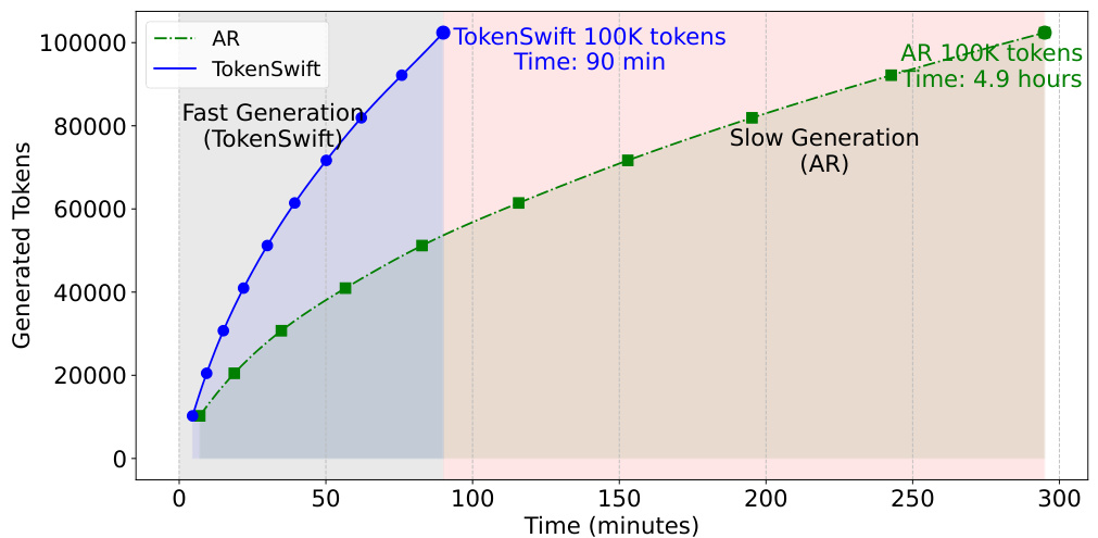
Figure 1. Comparison of the time taken to generate 100K tokens using auto regressive (AR) and TOKENSWIFT with prefix length of 4096 on LLaMA3.1-8b. As seen, TOKENSWIFT accelerates the AR process from nearly 5 hours to just 90 minutes.
图 1: 在 LLaMA3.1-8b 上使用自回归 (AR) 和 TOKENSWIFT (前缀长度为 4096) 生成 100K Token 所需时间的比较。如图所示,TOKENSWIFT 将 AR 过程从近 5 小时加速至仅 90 分钟。
1. Introduction
1. 引言
Recent advances in large language models (LLMs), amplified by their long context capacities (Wu et al., 2024; Ding et al., 2024), have demonstrated remarkable proficiency in intricate reasoning (Jaech et al., 2024; Guo et al., 2025), agentic thinking (Shinn et al., 2023; Yao et al., 2023; Li et al., 2024a), and creative writing (Wang et al.,
大语言模型 (LLMs) 的最新进展
2023; Mik hay lov ski y, 2023), etc. These advancements necessitate the ability to generate lengthy sequences, e.g., o1-like (Jaech et al., 2024) reasoning tends to generate protracted chain-of-thought trajectories before reaching final conclusions. However, a critical challenge impeding the practical deployment of such applications is the extensive time required to produce ultra-long sequences. For instance, generating 100K tokens with LLaMA3.1- 8B can take approximately five hours (Figure 1), a duration that is im practically long for the development of sophisticated applications, let alone recent gigantic models such as LLaMA3.1-405B (AI@Meta, 2024) and DeepSeek-600B (Liu et al., 2024a). Addressing this bottleneck is essential for harnessing the full potential of LLMs in real-world scenarios.
2023; Mik hay lov ski y, 2023) 等。这些进展需要生成长序列的能力,例如 o1-like (Jaech et al., 2024) 推理在得出结论之前往往会生成冗长的链式思维轨迹。然而,阻碍此类应用实际部署的一个关键挑战是生成超长序列所需的大量时间。例如,使用 LLaMA3.1-8B 生成 100K Token 可能需要大约五个小时 (图 1),这对于复杂应用的开发来说是不切实际的,更不用说最近的巨型模型如 LLaMA3.1-405B (AI@Meta, 2024) 和 DeepSeek-600B (Liu et al., 2024a) 了。解决这一瓶颈对于在现实场景中充分发挥大语言模型的潜力至关重要。
A straightforward solution is to take advantage of recent success in speculative decoding (SD) (Leviathan et al., 2023; Chen et al., 2023), which employs a draft-then-verify strategy to expedite generation while preserving lossless accuracy; see Appendix A and Section 5.1 for detailed background and relevant literature. However, these methods are generally tailored for generating short sequences, e.g., TriForce (Sun et al., 2024a) and MagicDec (Chen et al., 2024a) are limited to generating 256 and 64 tokens, respectively. Directly extending their generation length to 100K tokens would inevitably encounter failures due to KV cache budget constraints. Furthermore, even when applied to optimized KV cache architectures such as Group Query Attention (GQA), these methods yield only marginal acceleration gains for short-sequence generation, as evidenced in Tables 1 and 3. This observation leads to a pivotal research question:
一个直接的解决方案是利用推测解码 (Speculative Decoding, SD) 最近的成功 (Leviathan et al., 2023; Chen et al., 2023),该策略采用先起草后验证的方法来加速生成,同时保持无损精度;详细背景和相关文献请参见附录 A 和第 5.1 节。然而,这些方法通常是为生成短序列量身定制的,例如 TriForce (Sun et al., 2024a) 和 MagicDec (Chen et al., 2024a) 分别只能生成 256 和 64 个 Token。直接将它们的生成长度扩展到 100K Token 将不可避免地因 KV 缓存预算限制而遭遇失败。此外,即使应用于优化后的 KV 缓存架构,如群组查询注意力 (Group Query Attention, GQA),这些方法在短序列生成中也仅能带来微小的加速增益,如表 1 和表 3 所示。这一观察引出了一个关键的研究问题:
Is it possible to achieve model-agnostic lossless accelerations, akin to those seen in short-sequence SDs, for generating ultra-long sequences, with minimal training overhead?
是否可以在最小化训练开销的情况下,实现模型无关的无损加速,类似于在短序列 SD 中看到的效果,以生成超长序列?
To answer this question, we conduct an in-depth analysis (§2) and identify three key challenges: (1) frequent model reloading: frequently reloading model for each token generation introduces a significant delay, primarily due to memory access times rather than computation. (2) Prolonged Growing of KV Cache, the dynamic management of key-value (KV) pairs, which grow with the sequence length, adds complexity in maintaining model efficiency. (3) repetitive content generation, the issue of repetitive generation becomes more pronounced as the sequence length increases, leading to degraded output quality.
为了回答这个问题,我们进行了深入分析(§2),并确定了三个关键挑战:(1) 频繁的模型重载:为每个Token生成频繁重载模型会引入显著的延迟,这主要是由于内存访问时间而非计算。(2) KV缓存持续增长:随着序列长度的增加,键值对(KV)的动态管理增加了维护模型效率的复杂性。(3) 重复内容生成:随着序列长度的增加,重复生成问题变得更加明显,导致输出质量下降。
Building on these insights, we introduce our framework TOKENSWIFT, which utilizes $n$ -gram retrieval and dynamic KV cache updates to accelerate ultra-long sequence generation. Specifically, we employ multi-token generation and token re utilization to enable the LLM (i.e. target model) to draft multiple tokens in a single forward pass, alleviating the first challenge of frequent model reloading (§3.2). As the generation progresses, we dynamically update the partial KV cache at each iteration, reducing the KV cache loading time (§3.3). Finally, to mitigate the issue of repetitive outputs, we apply contextual penalty to constrain the generation process, ensuring the diversity of output (§3.4).
基于这些见解,我们提出了TOKENSWIFT框架,该框架利用$n$-gram检索和动态KV缓存更新来加速超长序列生成。具体来说,我们采用多Token生成和Token重用技术,使大语言模型(即目标模型)能够在一次前向传递中生成多个Token,从而缓解频繁模型重载的第一个挑战(§3.2)。随着生成的进行,我们在每次迭代中动态更新部分KV缓存,减少了KV缓存加载时间(§3.3)。最后,为了缓解输出重复的问题,我们应用上下文惩罚来约束生成过程,确保输出的多样性(§3.4)。
In $\S4_{,}$ , we conduct extensive experiments to evaluate TOKENSWIFT across different model scales and architectures. In summary, we highlight our advantages as:
在第4节中,我们进行了广泛的实验,以评估TOKENSWIFT在不同模型规模和架构上的表现。总结来说,我们的优势体现在:
- To the best of our knowledge, TOKENSWIFT is the first to accelerate ultra-long sequence generation up to 100K with lossless accuracy of target LLMs, while demonstrating significant superiority over enhanced baselines. 2. TOKENSWIFT consistently achieves over $\mathsfit{3\times}$ speedup compared to AR across varying prefix lengths, model architectures, and model scales in generating 100K tokens, reducing the AR process from nearly 5 hours to 90 minutes on LLaMA3.1-8b. 3. TOKENSWIFT achieves progressively higher speedup compared to AR as the generation length increases, while enhancing diversity in ultra-long sequence generation (as measured by Distinct-n (Li et al., 2016)).
- 据我们所知,TOKENSWIFT 是首个在加速超长序列生成(长达100K)的同时,保持目标大语言模型无损精度的技术,并在增强基线模型上展现出显著优势。
- TOKENSWIFT 在不同前缀长度、模型架构和模型规模下生成100K Token时,始终实现超过 $\mathsfit{3\times}$ 的加速,将LLaMA3.1-8b上的自回归 (AR) 过程从近5小时缩短至90分钟。
- TOKENSWIFT 在生成长度增加时,与AR相比实现了逐步更高的加速,同时增强了超长序列生成的多样性(通过Distinct-n (Li et al., 2016) 衡量)。
2. Challenges
2. 挑战
Accelerating long sequence generation is nevertheless a non-trivial task, even built upon prior success in speculative decoding (SD). In this section, we identify critical challenges encountered in accelerating ultra-long sequence generation.
加速长序列生成仍然是一个非平凡的任务,即使在推测解码(SD)之前的成功基础上也是如此。在本节中,我们识别了在加速超长序列生成过程中遇到的关键挑战。
Challenge I: Frequent Model Reloading One fundamental speed obstacle lies in the auto regressive (AR) generation scheme of LLM. For each token, the entire model must be loaded from GPU’s storage unit to the computing unit (Yuan et al., 2024), which takes significantly more time than the relatively small amount of computation performed (as shown in Table 2). Consequently, the primary bottleneck in generation stems from I/O memory access rather than computation.
挑战 I: 频繁的模型重载
一个根本的速度障碍在于大语言模型的自回归 (AR) 生成方案。对于每个 Token,整个模型必须从 GPU 的存储单元加载到计算单元 (Yuan et al., 2024),这比相对较少的计算量所花费的时间要多得多 (如表 2 所示)。因此,生成的主要瓶颈源于 I/O 内存访问而非计算。
Table 1. Experimental results of TriForce (Sun et al., 2024a) and MagicDec (Chen et al., 2024a) with default parameters on LLaMA3.1-8b. The Batch Size of MagicDec is set to 1.
表 1. TriForce (Sun 等, 2024a) 和 MagicDec (Chen 等, 2024a) 在 LLaMA3.1-8b 上使用默认参数的实验结果。MagicDec 的 Batch Size 设置为 1。
| 方法 | 生成长度 | 草稿形式 | 加速比 |
|---|---|---|---|
| TriForce | 256 | 独立草稿 | 1.02 |
| MagicDec | 64 | 自我推测 | 1.20 |
| MagicDec | 64 | 独立草稿 | 1.06 |
Table 2. Taking NVIDIA A100 80G and LLaMA3.1-8b as example, MAX refers to the scenario with a maximum context window 128K. The calculation method is from Yuan et al. (2024).
表 2: 以 NVIDIA A100 80G 和 LLaMA3.1-8b 为例,MAX 表示最大上下文窗口为 128K 的场景。计算方法来自 Yuan 等人 (2024)。
| 内存 | 计算 |
|---|---|
| 带宽:2.04e12B/s | BF16:312e12FLOPS |
| 模型权重:15.0 GB | 最大操作数:83.9GB |
| 加载时间:7.4ms | 最大计算时间:0.3ms |
▷ When generating ultra-long sequence, such as 100K tokens, the GPU must reload the model weights over 100,000 times. This repetitive process poses the challenge: How can we reduce the frequency of model reloading?
▷ 在生成超长序列(例如 100K Token)时,GPU 必须重新加载模型权重超过 10 万次。这一重复过程带来了挑战:我们如何减少模型重新加载的频率?
Challenge II: Prolonged Growing of KV Cache Previous studies, such as TriForce (Sun et al., 2024a) and MagicDec (Chen et al., 2024a) have demonstrated that, a small KV cache budget can be used during the drafting phase to reduce the time increase caused by the loading enormous KV cache. While their one-time compression strategy at the prefill stage can handle scenarios with long prefixes and short outputs, it fails to address cases involving ultra-long outputs, as the growing size of KV cache would far exceed the allocated length budget.
挑战二:KV缓存的持续增长
先前的研究,如TriForce (Sun et al., 2024a) 和 MagicDec (Chen et al., 2024a) 已经证明,在草拟阶段可以使用较小的KV缓存预算来减少因加载庞大KV缓存而增加的时间。虽然它们在预填充阶段的一次性压缩策略可以处理长前缀和短输出的场景,但无法应对超长输出的情况,因为KV缓存不断增长的规模将远远超过分配的长度预算。
$\triangleright T o$ dynamically manage partial KV cache within limited budget during ultra-long sequence generation, the challenge lies in determining when and how to dynamically update the KV cache.
$\triangleright T o$ 在超长序列生成过程中,如何在有限的预算内动态管理部分 KV 缓存,其挑战在于确定何时以及如何动态更新 KV 缓存。
Challenge III: Repetitive Content Generation The degeneration of AR in text generation tasks — characterized by output text that is bland, incoherent, or gets stuck in repetitive loops — is a widely studied challenge (Holtzman et al., 2020; Nguyen et al., 2024; Hewitt et al., 2022). When generating sequences of considerable length, e.g., 100K, the model tends to produce repetitive sentences (Figure 5).
挑战 III:重复内容生成
AR(自回归)在文本生成任务中的退化问题——表现为生成文本平淡、不连贯或陷入重复循环——是一个被广泛研究的挑战(Holtzman et al., 2020; Nguyen et al., 2024; Hewitt et al., 2022)。当生成长度较长的序列时,例如 100K,模型往往会生成重复的句子(图 5)。
$\vartriangleright$ Since our objective is lossless acceleration and repetition is an inherent problem in LLMs, eliminating this issue is not our focus. However, it is still essential and challenging to mitigate repetition patterns in ultra-long sequences.
$\vartriangleright$ 由于我们的目标是无损加速,而重复是大语言模型中的一个固有问题,因此消除这一问题并非我们的重点。然而,在超长序列中减轻重复模式仍然是至关重要且具有挑战性的。
3. TOKENSWIFT
3. TOKENSWIFT
To achieve lossless acceleration in generating ultra-long sequences, we propose tailored solutions for each challenge inherent to this process. These solutions are seamlessly integrated into a unified framework, i.e. TOKENSWIFT.
为了实现超长序列生成中的无损加速,我们针对这一过程中固有的每个挑战提出了定制化的解决方案。这些解决方案被无缝集成到一个统一的框架中,即 TOKENSWIFT。
3.1. Overview
3.1. 概述
The overall framework is depicted in Figure 2. TOKENSWIFT generate a sequence of draft tokens with selfdrafting, which are then passed to the target (full) model for validation using a tree-based attention mechanism (See Appendix E for more tree-based attention details). This process ensures that the final generated output aligns with the target model’s predictions, effectively achieving lossless acceleration.
整体框架如图 2 所示。TOKENSWIFT 通过自生成生成一系列草稿 Token,然后使用基于树的注意力机制(详见附录 E)将这些 Token 传递给目标(完整)模型进行验证。这一过程确保最终生成的输出与目标模型的预测一致,从而实现无损加速。
OKENSWIFT is lightweight because the draft model is the target model itself with a partial KV cache. This eliminates the need to train a separate draft LLM; instead, only $\gamma$ linear layers need to be trained, where $\gamma+1^{1}$ represents the number of logits predicted in a single forward pass. In addition, during the verification process, once we obtain the target tokens from the target model with full KV cache, we directly compare draft tokens with target tokens sequentially to ensure that the process is lossless (He et al., 2024).
TOKENSWIFT 之所以轻量,是因为草稿模型本身就是目标模型,只是带有部分 KV 缓存。这消除了训练独立草稿大语言模型的需求;相反,只需训练 $\gamma$ 个线性层,其中 $\gamma+1^{1}$ 表示单次前向传播中预测的 Logits 数量。此外,在验证过程中,一旦我们从带有完整 KV 缓存的目标模型中获取目标 Token,我们会依次将草稿 Token 与目标 Token 直接比较,以确保过程无损 (He et al., 2024)。
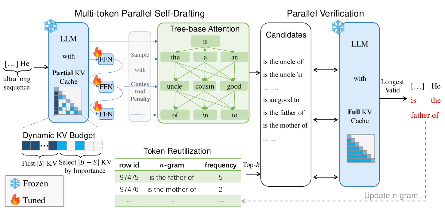
Figure 2. Illustration of TOKENSWIFT Framework. First, target model (LLM) with partial KV cache and three linear layers outputs 4 logits in a single forward pass. Tree-based attention is then applied to construct candidate tokens. Secondly, top $k$ candidate 4-grams are retrieved accordingly. These candidates compose draft tokens, which are fed into the LLM with full KV cache to generate target tokens. The verification is performed by checking if draft tokens match exactly with target tokens (Algorithm 1). Finally, we randomly select one of the longest valid draft tokens, and update $n$ -gram table and KV cache accordingly.
图 2: TOKENSWIFT 框架示意图。首先,具有部分 KV 缓存和三个线性层的目标模型(大语言模型)在单次前向传播中输出 4 个 logits。然后应用基于树的注意力机制来构建候选 token。其次,相应地检索前 $k$ 个候选 4-gram。这些候选组成草稿 token,并将其输入具有完整 KV 缓存的大语言模型中以生成目标 token。验证通过检查草稿 token 是否与目标 token 完全匹配来进行(算法 1)。最后,我们随机选择一个最长的有效草稿 token,并相应地更新 $n$-gram 表和 KV 缓存。
3.2. Multi-token Generation and Token Re utilization
3.2. 多Token生成与Token重用
Multi-token Self-Drafting Inspired by Medusa (Cai et al., 2024), we enable the LLM to generate multiple draft tokens in a single forward pass by incorporating $\gamma$ additional linear layers. However, we empirically note that the additional linear layers should not be independent of each other. Specifically, we propose the following structure:
多Token自草稿生成

where $h_{0}$ denotes the last hidden state of LLM, $f_{i}(\cdot)$ represents the $i$ -th linear layer, $h_{i}$ refers to the $i\cdot$ -th hidden representation, $g(\cdot)$ represents the LM Head of target model, and $l_{i}$ denotes output logits. This structure aligns more closely with the AR nature of the model. Moreover, this adjustment incurs no additional computational cost.
其中 $h_{0}$ 表示大语言模型的最后一个隐藏状态,$f_{i}(\cdot)$ 表示第 $i$ 个线性层,$h_{i}$ 表示第 $i$ 个隐藏表示,$g(\cdot)$ 表示目标模型的 LM Head,$l_{i}$ 表示输出的 logits。这种结构更符合模型的 AR 特性。此外,这种调整不会产生额外的计算成本。
Token Re utilization Given the relatively low acceptance rate of using linear layers to generate draft tokens, we propose a method named token re utilization to further reduce the frequency of model reloads. The idea behind token re utilization is that some phrases could appear frequently, and they are likely to reappear in subsequent generations.
Token 重复利用
Specifically, we maintain a set of tuples ${(\mathcal{G},\mathcal{F})},$ where $\mathcal{G}={x_{i+1},...,x_{i+n}}$ represents an $n$ -gram and $\mathcal{F}$ denotes its corresponding frequency $\mathcal{F}$ within the generated token sequence ${\cal{S}}={x_{0},x_{1},...,x_{t-1}}$ by time step $t\left(t\geqslant n\right)$ . After obtaining ${p_{0},\ldots,p_{3}}$ as described in $\S3.4,$ we retrieve the top $k$ most frequent $n$ -grams beginning with
具体来说,我们维护一组元组 ${(\mathcal{G},\mathcal{F})},$ 其中 $\mathcal{G}={x_{i+1},...,x_{i+n}}$ 表示一个 $n$ -gram,而 $\mathcal{F}$ 表示其在生成 Token 序列 ${\cal{S}}={x_{0},x_{1},...,x_{t-1}}$ 中到时间步 $t\left(t\geqslant n\right)$ 为止的对应频率 $\mathcal{F}$。在按照 $\S3.4$ 所述获取 ${p_{0},\ldots,p_{3}}$ 后,我们检索以这些概率开头的前 $k$ 个最频繁的 $n$ -grams。
token arg max $p_{0}$ to serve as additional draft tokens.
token arg max $p_{0}$ 作为额外的草稿 token。
Although this method can be applied to tasks with long prefixes, its efficacy is constrained by the limited decoding steps, which reduces the opportunities for accepting $n$ -gram candidates. Additionally, since the long prefix text is not generated by the LLM itself, a distribution al discrepancy exists between the generated text and the authentic text (Mitchell et al., 2023). As a result, this method is particularly suitable for generating ultra-long sequences.
尽管该方法可应用于具有长前缀的任务,但其效果受限于有限的解码步骤,这减少了接受 $n$ 元候选词的机会。此外,由于长前缀文本并非由大语言模型自身生成,生成文本与真实文本之间存在分布差异 (Mitchell et al., 2023)。因此,该方法特别适合生成超长序列。
3.3. Dynamic KV Cache Management
3.3. 动态 KV 缓存管理
Dynamic KV Cache Updates Building upon the findings of Xiao et al. (2024), we preserve the initial $|S|$ KV pairs within the cache during the drafting process, while progressively evicting less important KV pairs. Specifically, we enforce a fixed budget size $|B|,$ ensuring that the KV cache at any given time can be represented as:
动态KV缓存更新基于Xiao等人(2024)的研究成果,我们在草拟过程中保留缓存中的初始$|S|$个KV对,同时逐步淘汰重要性较低的KV对。具体而言,我们强制执行固定预算大小$|B|$,确保在任何给定时间点的KV缓存可以表示为:

where the first $|S|$ pairs remain fixed, and the pairs from position $|S|$ to $|B|-1$ are ordered by decreasing importance. As new tokens are generated, less important KV pairs are gradually replaced, starting from the least important ones at position $|B|-1$ and moving towards position $|S|$ . Once replacements extend beyond the |S| position, we re calculate the importance scores of all preceding tokens and select the most relevant $\left|B\right|-\left|S\right|$ pairs to reconstruct the cache. This process consistently preserves the critical information required for ultra-long sequence generation.
其中前 $|S|$ 对保持固定,从位置 $|S|$ 到 $|B|-1$ 的对按重要性递减排序。随着新 Token 的生成,从位置 $|B|-1$ 开始,逐渐替换重要性较低的 KV 对,直到位置 $|S|$。一旦替换超过 |S| 位置,我们会重新计算所有前导 Token 的重要性分数,并选择最相关的 $\left|B\right|-\left|S\right|$ 对来重建缓存。这一过程始终保留超长序列生成所需的关键信息。
Importance Score of KV pairs We rank the KV pairs based on the importance scores derived from the dot product between the query (Q) and key (K), i.e. ${\bf Q}{\bf K}^{\overleftarrow{T}}$ .
键值对重要性评分
In the case of Group Query Attention (GQA), since each K corresponds to a group of $\mathcal{Q}={\mathbf{Q}{0},...,\mathbf{Q}{g-1}},$ direct dot-product computation is not feasible. Unlike methods such as SnapKV (Li et al., 2024c), we do not replicate the K. Instead, we partition the $\mathcal{Q},$ as shown in Equation (2):
在 Group Query Attention (GQA) 的情况下,由于每个 K 对应一组 $\mathcal{Q}={\mathbf{Q}{0},...,\mathbf{Q}{g-1}},$ 直接进行点积计算是不可行的。与 SnapKV (Li et al., 2024c) 等方法不同,我们不会复制 K。相反,我们对 $\mathcal{Q},$ 进行分区,如公式 (2) 所示:

where for position $i,\mathbf{Q}{j}$ in the group $\mathcal{Q}{i}$ are dot-product with the same $\mathbf{K}_{i},$ and their results are aggregated to obtain the final importance score. This approach enhances memory saving while preserving the quality of the attention mechanism, ensuring that each query is effectively utilized without introducing unnecessary redundancy.
其中对于位置 $i,\mathcal{Q}{i}$ 组中的 $\mathbf{Q}{j}$ 与相同的 $\mathbf{K}_{i},$ 进行点积,并将结果聚合以获得最终的重要性分数。这种方法在保持注意力机制质量的同时增强了内存节省,确保每个查询都被有效利用而不引入不必要的冗余。
3.4. Contextual Penalty and Random N-gram Selection
3.4. 上下文惩罚与随机 N-gram 选择
The penalized sampling approach proposed in (Keskar et al., 2019) suggests applying a penalty to all generated tokens. However, when generating ultra-long sequences, the set of generated tokens may cover nearly all common words, which limits the ability to sample appropriate tokens. Therefore, we propose an improvement to this method.
(Keskar et al., 2019) 提出的惩罚采样方法建议对所有生成的 Token 施加惩罚。然而,在生成超长序列时,生成的 Token 集可能几乎覆盖所有常见单词,这限制了采样合适 Token 的能力。因此,我们对该方法提出改进。
Specifically, we introduce a fixed penalty window W and apply penalty value $\theta$ to the most recent $W$ tokens, denoted as $\mathbb{W}$ , generated up to the current position, as illustrated in Equation (3):
具体来说,我们引入了一个固定的惩罚窗口 W,并对最近生成的 W 个 Token(记为 $\mathbb{W}$)应用惩罚值 $\theta$,如公式 (3) 所示:
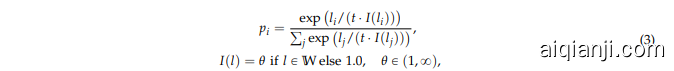
where $t$ denotes temperature, $l_{i}$ and $p_{i}$ represent the logit and probability of $i$ -th token. This adjustment aims to maintain diversity while still mitigating repetitive generation.
其中 $t$ 表示温度,$l_{i}$ 和 $p_{i}$ 分别表示第 $i$ 个 Token 的 logit 和概率。此调整旨在保持多样性的同时,减少重复生成。
Algorithm 1 TOKENSWIFT
算法 1 TOKENSWIFT
Random $n$ -gram Selection In our experiments, we observe that the draft tokens provided to the target model for parallel validation often yield multiple valid groups. Building on this observation, we randomly select one valid $n$ -gram to serve as the final output. By leveraging the fact that multiple valid $n$ -grams emerge during verification, we ensure that the final output is both diverse and accurate.
随机 $n$ -gram 选择
In summary, the overall flow of our framework is presented in Algorithm 1.
总之,我们的框架的整体流程在算法 1 中展示。
4. Experiments
4. 实验
In this section, we demonstrate the capability of TOKENSWIFT in accelerating ultra-long sequences generation.
在本节中,我们展示了TOKENSWIFT在加速超长序列生成方面的能力。
4.1. Setup
4.1. 设置
We conduct experiments on a variety of models, including YaRN-LLaMA2-7b-128k (Peng et al., 2024), LLaMA3.1-8b (AI@Meta, 2024) and Qwen2.5-(1.5b,7b,14b) (Qwen et al., 2025). For all models, we use the Base version, as the output length of Instruct version is limited (Bai et al., 2024). The inference experiments are performed on the test set of PG-19 (Rae et al., 2020).
我们在多种模型上进行了实验,包括 YaRN-LLaMA2-7b-128k (Peng 等, 2024)、LLaMA3.1-8b (AI@Meta, 2024) 和 Qwen2.5-(1.5b,7b,14b) (Qwen 等, 2025)。对于所有模型,我们均使用基础版本,因为指导版本的输出长度有限 (Bai 等, 2024)。推理实验在 PG-19 (Rae 等, 2020) 的测试集上进行。
Training and Inference Details We train linear layers in Section 3.2 using the first 8K tokens of training data, for datasets longer than 8K tokens, from PG-19 (Rae et al., 2020). The number of extra decoding heads is set to 3 across all models.
训练与推理细节
我们使用 PG-19 (Rae et al., 2020) 数据集中前 8K Token 的训练数据来训练第 3.2 节中的线性层,对于超过 8K Token 的数据集也是如此。所有模型的额外解码头数量均设置为 3。
Inference is performed on a single NVIDIA A100-SXM4-80GB. When generating 100K tokens, the models are prefilled with 2K, 4K or 8K tokens as prompt from a random sample of the PG-19 test set (See Appendix F.2 for ablation on prefill length). The maximum budget of the partial cache is determined by the length of the prompt. For further training and inference details, please refer to Appendix B.
推理在单个 NVIDIA A100-SXM4-80GB 上进行。当生成 100K 个 Token 时,模型会从 PG-19 测试集的随机样本中预填充 2K、4K 或 8K 个 Token 作为提示(有关预填充长度的消融实验,请参见附录 F.2)。部分缓存的最大预算由提示的长度决定。有关进一步训练和推理的详细信息,请参阅附录 B。
Evaluation Metrics We evaluate the overall acceptance rate and speedup for all methods. Unlike Leviathan et al. $(2023)^{3}$ , our acceptance rate α is defined as:
评估指标
Table 3. Experimental results for LLaMA2 and LLaMA3.1 under varying prefix lengths, generating sequences from 20K to 100K tokens. α denotes the acceptance rate of all draft tokens (Equation (4)), while $\times$ represents the speedup ratio relative to AR (Equation (5)). TriForce* refers to our improved version, and Medusa* indicates the model we retrained (§4.1).
表 3: LLaMA2 和 LLaMA3.1 在不同前缀长度下的实验结果,生成序列从 20K 到 100K Tokens。α 表示所有草稿 Tokens 的接受率 (公式 (4)),而 $\times$ 表示相对于 AR 的加速比 (公式 (5))。TriForce* 指我们改进的版本,Medusa* 表示我们重新训练的模型 (§4.1)。
| 方法 | 生成长度 | 预填充长度 2048 | 预填充长度 4096 | 预填充长度 8192 | 预填充长度 2048 | 预填充长度 4096 | 预填充长度 8192 |
|---|---|---|---|---|---|---|---|
| YaRN-LLaMA2-7b-128k (MHA) | LLaMA3.1-8b (GQA) | ||||||
| α | ×(>1) | α | ×(>1) | α | ×(>1) | ||
| Medusa* | 20K | 0.43 | 0.96 | 0.39 | 0.85 | 0.40 | 0.83 |
| TriForce* | 20K | 0.80 | 1.50 | 0.89 | 1.51 | 0.92 | 1.36 |
| TOKENSWIFT | 20K | 0.73±0.09 | 2.11±0.14 | 0.68±0.09 | 2.02±0.20 | 0.64±0.08 | 1.91±0.12 |
| Medusa* | 40K | 0.52 | 1.08 | 0.42 | 0.86 | 0.43 | 0.88 |
| TriForce* | 40K | 0.84 | 1.64 | 0.93 | 1.67 | 0.96 | 1.49 |
| TOKENSWIFT | 40K | 0.82±0.06 | 2.60±0.05 | 0.79±0.06 | 2.56±0.09 | 0.79±0.05 | 2.50±0.07 |
| Medusa* | 60K | 0.59 | 1.18 | 0.47 | 0.95 | 0.45 | 0.91 |
| TriForce* | 60K | 0.85 | 1.76 | 0.95 | 1.83 | 0.97 | 1.62 |
| TOKENSWIFT | 60K | 0.87±0.04 | 2.92±0.04 | 0.85±0.04 | 2.89±0.06 | 0.85±0.04 | 2.84±0.05 |
| Medusa* | 80K | 0.61 | 1.17 | 0.51 | 0.99 | 0.47 | 0.93 |
| TriForce* | 80K | 0.84 | 1.86 | 0.95 | 1.98 | 0.97 | 1.74 |
| TOKENSWIFT | 80K | 0.89±0.03 | 3.13±0.04 | 0.88±0.04 | 3.10±0.06 | 0.88±0.03 | 3.05±0.03 |
| Medusa* | 100K | 0.62 | 1.15 | 0.52 | 0.99 | 0.47 | 0.91 |
| TriForce* | 100K | 0.82 | 1.94 | 0.96 | 2.14 | 0.97 | 1.86 |
| TOKENSWIFT | 100K | 0.90±0.02 | 3.25±0.05 | 0.90±0.03 | 3.23±0.06 | 0.90±0.02 | 3.20±0.02 |
where $a_{i}$ represents the number of tokens accepted at the $i\cdot$ -th time step, $\gamma+1$ denotes the number of draft tokens generated at each time step, and $T$ represents the total number of time steps. The speedup is denotes as $\times,$ which is the ratio of AR latency to TOKENSWIFT latency, given by:
其中 $a_{i}$ 表示在第 $i\cdot$ 个时间步接受的 token 数量,$\gamma+1$ 表示每个时间步生成的草稿 token 数量,$T$ 表示总时间步数。加速比表示为 $\times,$ 它是 AR 延迟与 TOKENSWIFT 延迟的比值,由下式给出:

where latency refers to the average time required to generate a single token.
其中延迟指的是生成单个Token所需的平均时间。
We use Distinct $n$ (Li et al., 2016) to measure the diversity of generated content, i.e., repetition. A higher value indicates greater diversity and lower repetition (Table 6).
我们使用 Distinct $n$ (Li et al., 2016) 来衡量生成内容的多样性,即重复性。值越高表示多样性越大,重复性越低(表 6)。
Baselines We compare TOKENSWIFT with two baselines: TriForce*: The original TriForce (Sun et al., 2024a) employs a static KV update strategy, which cannot accelerate the generation of 100K tokens. The results in Table 3 correspond to our improved version of TriForce, which incorporates dynamic KV update . Medusa*: To ensure lossless ness, we adopt the Medusa (Cai et al., 2024) training recipe and incorporate the verification method of TOKENSWIFT. Both Medusa heads and tree structure are consistent with TOKENSWIFT.
基线方法 我们将TOKENSWIFT与两种基线方法进行比较:TriForce*:原始TriForce(Sun et al., 2024a)采用静态KV更新策略,无法加速生成100K个Token。表3中的结果对应我们改进后的TriForce版本,该版本加入了动态KV更新。Medusa*:为了确保无损性,我们采用了Medusa(Cai et al., 2024)的训练方法,并融入了TOKENSWIFT的验证方法。Medusa的头部和树结构均与TOKENSWIFT一致。
The recent released MagicDec (Chen et al., 2024a) primarily focuses on acceleration for large throughput, and when the batch size is 1, LLaMA3.1-8b does not exhibit any acceleration for short text generation, let alone for ultra-long sequences. Therefore, it is excluded from our baseline.
近期发布的 MagicDec (Chen et al., 2024a) 主要关注大吞吐量的加速,当批次大小为 1 时,LLaMA3.1-8b 在短文本生成上并未表现出任何加速效果,更不用说超长序列了。因此,它被排除在我们的基线之外。
4.2. Main Results
4.2. 主要结果
The experimental results are presented in Table 3 and Table 4. We evaluate TOKENSWIFT at different generation lengths of 20K, 40K, 60K, 80K and 100K, reporting speedup $\times$ and acceptance rate $\alpha$ by taking the average and standard deviation of 5 experiments to avoid randomness. Notably, the results for TOKENSWIFT and Medusa* show a balanced trade-off between speed and quality, in contrast to TriForce*, which suffers from low quality due to the absence of any repetition penalty.
实验结果如表 3 和表 4 所示。我们在 20K、40K、60K、80K 和 100K 的不同生成长度下评估了 TOKENSWIFT,报告了加速比 $\times$ 和接受率 $\alpha$,并通过取 5 次实验的平均值和标准差来避免随机性。值得注意的是,TOKENSWIFT 和 Medusa* 的结果在速度和质量之间表现出平衡的权衡,而 TriForce* 由于缺乏任何重复惩罚,导致质量较低。
TOKENSWIFT significantly outperforms all baselines across generation lengths. As shown in Table 3, across all engths, TOKENSWIFT demonstrates superior acceleration performance compared to all baselines on models with
TOKENSWIFT在各生成长度上显著优于所有基线模型。如表 3 所示,在所有长度上,TOKENSWIFT在模型上展现出比所有基线更优越的加速性能。
4To compare with LLaMA3.1-8b, we pretrained a draft model based on LLaMA3.1-8b. See Appendix C for details.
为了与 LLaMA3.1-8b 进行比较,我们基于 LLaMA3.1-8b 预训练了一个草稿模型。详见附录 C。
Table 4. Experimental results of TOKENSWIFT for Qwen2.5 across different scales under prefix length 4096, generating sequences from 20K to 100K tokens. $T_{A R}$ and T TOKEN SWIFT denote the actual time required (in minutes) for AR and TOKENSWIFT, respectively. $\Delta_{T}$ represents the number of minutes saved by TOKENSWIFT compared to AR.
表 4: 不同规模下 Qwen2.5 模型在前缀长度为 4096 时,生成 20K 到 100K Token 序列的 TOKENSWIFT 实验结果。$T_{A R}$ 和 $T_{TOKENSWIFT}$ 分别表示 AR 和 TOKENSWIFT 实际所需的时间(分钟)。$\Delta_{T}$ 表示 TOKENSWIFT 相比 AR 节省的时间(分钟)。
| Gen.Len. | Qwen2.5-1.5B | x(> 1) | TAR | TTOKENSWIFT | △T | Qwen2.5-7B | x(> 1) | TAR | TTOKENSWIFT | △T | α | Qwen2.5-14B | x(> 1) | TAR | TTOKENSWIFT | △T | ||||
|---|---|---|---|---|---|---|---|---|---|---|---|---|---|---|---|---|---|---|---|---|
| 20K | 0.69±0.11 | 1.69±0.17 | 12.00 | 7.20 | -4.80 | 0.64±0.07 | 2.00±0.16 | 15.60 | 7.80 | -7.80 | 0.67±0.06 | 2.12±0.13 | 29.40 | 13.80 | -15.60 | |||||
| 40K | 0.80±0.06 | 2.31±0.09 | 36.00 | 15.60 | -20.40 | 0.77±0.05 | 2.64±0.10 | 47.40 | 18.00 | -29.40 | 0.78±0.03 | 2.68±0.10 | 89.40 | 33.60 | -55.80 | |||||
| 60K | 0.85±0.04 | 2.69±0.07 | 73.80 | 27.60 | -46.20 | 0.78±0.08 | 2.86±0.25 | 95.40 | 33.60 | -61.80 | 0.82±0.02 | 23.01±0.13 | 184.20 | 61.20 | -123.00 | |||||
| 80K | 0.87±0.03 | 2.95±0.06 | 124.20 | 42.00 | -82.20 | 0.80±0.09 | 3.07±0.30 | 161.40 | 52.80 | -108.60 | 0.83±0.02 | 23.20±0.13 | 312.60 | 97.80 | -214.80 | |||||
| 100K | 0.89±0.07 | 3.13±0.07 | 187.80 | 60.00 | -127.80 | 0.82±0.09 | 3.23±0.28 | 244.20 | 75.60 | -168.60 | 0.84±0.02 | 3.34±0.10 | 474.60 | 142.20 | -332.40 |
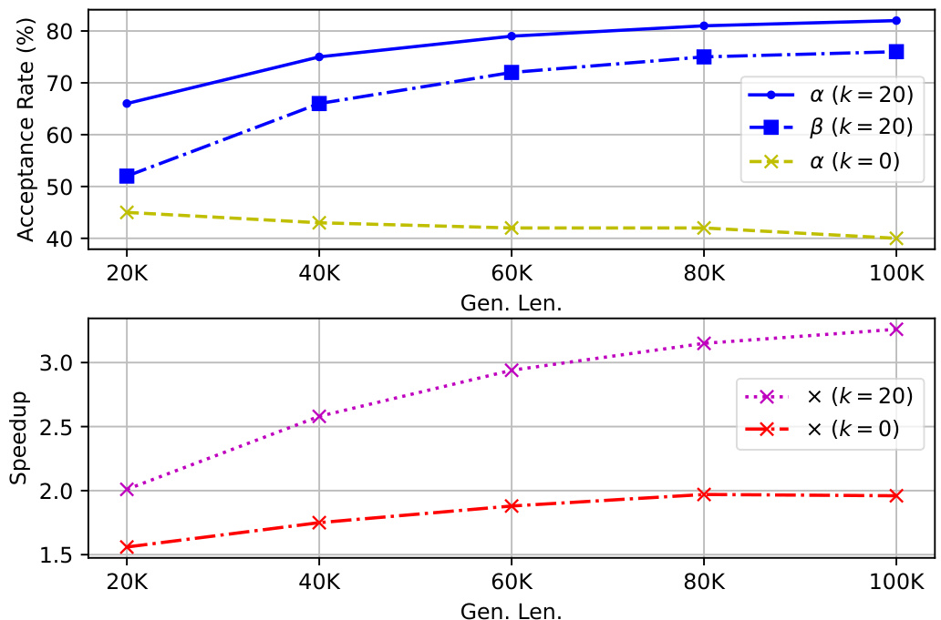
Figure 3. Upper: The acceptance rate α for $k=20$ and $k=0$ , along with the $n$ -gram acceptance rate $\beta$ for $k=20$ , plotted against varying generation lengths. Lower: The speedup $\times$ achieved at different generation lengths.
图 3: 上:$k=20$ 和 $k=0$ 的接受率 $\alpha$,以及 $k=20$ 的 $n$-gram 接受率 $\beta$,随生成长度变化的情况。下:不同生成长度下实现的加速倍数 $\times$。
different architectures (MHA, GQA). Moreover, TOKENSWIFT demonstrates remarkable robustness, showing virtually no impact when tested with varying prefix lengths.
不同架构 (MHA, GQA)。此外,TOKENSWIFT 表现出显著的鲁棒性,在使用不同前缀长度进行测试时几乎不受影响。
Longer generations amplify the speedup benefits. As the generation length increases, the speed improvement of TOKENSWIFT becomes increasingly evident. Two key factors drive this trend: Firstly, AR experiences longer KV cache loading times as the number of tokens grows, whereas TOKENSWIFT mitigates this issue by utilizing dynamic KV pruning. Secondly, the acceptance rate improves as the number of tokens increases, primarily due to the higher $n$ -grams acceptance rate. As the $n$ -grams pool composed of generated tokens grows larger, the candidate $n$ -grams become more diverse and accurate (Figure 3).
生成长度越长,TOKENSWIFT 的加速优势越明显。随着生成长度的增加,TOKENSWIFT 的速度提升变得越来越显著。这一趋势主要由两个关键因素驱动:首先,随着 token 数量的增加,AR 的 KV 缓存加载时间变长,而 TOKENSWIFT 通过动态 KV 剪枝缓解了这一问题。其次,随着 token 数量的增加,接受率提高,这主要归因于更高的 $n$ -grams 接受率。随着由生成的 token 组成的 $n$ -grams 池变得更大,候选 $n$ -grams 变得更加多样化和准确(图 3)。
Larger models yield greater speedup benefits. The impact of frequent model reloading varies with model scale, as larger models require more time due to the increased parameters. As shown in Table 4, TOKENSWIFT demonstrates robust performance across models of different scales, with the acceleration advantage becoming more pronounced for larger models. In particular, when generating 100K tokens, TOKENSWIFT saves up to 5.54 hours for 14B model.
更大规模的模型带来更显著的加速效益。频繁的模型重载影响因模型规模而异,因为更大的模型由于参数增多而需要更多时间。如表 4 所示,TOKENSWIFT 在不同规模的模型上均表现出稳健的性能,且对更大模型的加速优势更为明显。特别是当生成 100K tokens 时,TOKENSWIFT 为 14B 模型节省了多达 5.54 小时。
4.3. Ablation Studies
4.3. 消融研究
We conduct comprehensive ablation studies on TOKENSWIFT using LLaMA3.1-8b. For all experiments, the prefix length is 4096.
我们使用 LLaMA3.1-8b 对 TOKENSWIFT 进行了全面的消融研究。所有实验中,前缀长度均为 4096。
4.3.1. TOKEN RE UTILIZATION
4.3.1. Token 重复利用
We define the $n$ -gram acceptance rate $\beta$ similarly to Equation (4). Let $a_{i}^{\prime}$ denote the length of accepted $n$ -gram candidate at iteration $i$ . Then $\beta$ is given by:
我们定义 $n$ -gram 接受率 $\beta$ 与公式 (4) 类似。设 $a_{i}^{\prime}$ 表示在第 $i$ 次迭代时接受的 $n$ -gram 候选长度,则 $\beta$ 由下式给出:

From Figure 3, we observe that removing token re utilization $(k=0)$ ) leads to a significant decrease in both acceptance rate $\alpha$ and speedup $\times$ . Furthermore, as the generation length increases, the acceptance rate $\alpha$ for $k=0$ slightly drops. This trend stems from the fact that, in ultra-long sequences, the KV cache cannot be compressed indefinitely. In contrast, TOKENSWIFT $(k=20)$ ) shows an increasing acceptance rate as the sequence length grows, demonstrating the effectiveness of token re utilization in reducing the frequency of model reloading.
从图 3 中我们观察到,移除 token 重用 $(k=0)$ 会导致接受率 $\alpha$ 和加速比 $\times$ 显著下降。此外,随着生成长度的增加,$k=0$ 的接受率 $\alpha$ 略有下降。这一趋势源于在超长序列中,KV 缓存无法无限压缩。相比之下,TOKENSWIFT $(k=20)$ 的接受率随着序列长度的增加而上升,展示了 token 重用在减少模型重新加载频率方面的有效性。
Table 5. The ablation experiment results on KV management.
表 5. KV管理的消融实验结果
| Gen.Len. | 全缓存 | 部分缓存 | 动态部分缓存 | |
|---|---|---|---|---|
| 20K | α | 0.42 | 0.19 | 0.45 |
| ×(>1) | 1.36 | 0.94 | 1.56 | |
| 40K | α | 0.42 | 0.16 | 0.43 |
| ×(>1) | 1.42 | 1.03 | 1.75 | |
| 60K | α | 0.42 | 0.18 | 0.42 |
| ×(>1) | 1.45 | 1.19 | 1.88 | |
| 80K | α | 0.42 | 0.19 | 0.42 |
| ×(>1) | 1.46 | 1.31 | 1.97 | |
| 100K | α | 0.42 | 0.21 | 0.40 |
| ×(>1) | 1.47 | 1.44 | 1.96 |
Table 6. The ablation experiment results on contextual penalty using different sampling methods. Light cell represents the settings adopted by TOKENSWIFT. We take $\theta=1.2$ , $W=$ 1024.
表 6: 使用不同采样方法的上下文惩罚消融实验结果。浅色单元格表示 TOKENSWIFT 采用的设置。我们取 $\theta=1.2$,$W=1024$。
| Distinct-1 | Distinct-2 | Distinct-3 | Distinct-4 | AVG. | X | |
|---|---|---|---|---|---|---|
| top-p w/o.penalty | 0.15 | 0.25 | 0.29 | 0.31 | 0.25 | 3.42 |
| 0.09 | 0.15 | 0.18 | 0.20 | 0.16 | 3.53 | |
| r-sampling w/o.penalty | 0.25 | 0.43 | 0.49 | 0.53 | 0.43 | 3.42 |
| 0.06 | 0.10 | 0.12 | 0.13 | 0.11 | 3.57 | |
| min-p w/o.penalty | 0.41 | 0.71 | 0.81 | 0.82 | 0.69 | 3.27 |
| 0.07 | 0.11 | 0.14 | 0.15 | 0.12 | 3.58 |
4.3.2. DYNAMIC KV UPDATES
4.3.2. 动态KV更新
To evaluate the effectiveness of TOKENSWIFT’s dynamic KV update policy, we experiment with three different strategies of managing KV cache during drafting:
为了评估TOKENSWIFT的动态KV更新策略的有效性,我们实验了三种不同的草稿生成过程中管理KV缓存的策略:
‚ Full Cache: Retaining full KV cache throughout drafting. ‚ Partial Cache: Updating partial KV cache only once during the prefill phase. ‚ Dynamic Partial Cache: Dynamically updating KV cache as described in $\S3.3$
- 全缓存:在整个起草阶段保留完整的KV缓存。
- 部分缓存:在预填充阶段仅更新部分KV缓存。
- 动态部分缓存:如 $\S3.3$ 所述,动态更新KV缓存。
For a fair comparison, token re utilization is disabled (i.e. $k=0$ ). As shown in Table 5, Partial Cache leads to a low acceptance rate, resulting in reduced speedup. While Full Cache achieves a higher acceptance rate, its computational overhead negates the speedup gains. In contrast, Dynamic Partial Cache adopted by TOKENSWIFT strikes a balanced trade-off, achieving both high acceptance rate and significant speedup. As a result, Dynamic Partial Cache can effectively manage partial KV under ultra-long sequence generation.
为了公平比较,Token 重复利用被禁用(即 $k=0$)。如表 5 所示,Partial Cache 导致接受率较低,从而降低了加速效果。而 Full Cache 实现了较高的接受率,但其计算开销抵消了加速收益。相比之下,TOKENSWIFT 采用的 Dynamic Partial Cache 实现了平衡的权衡,既达到了高接受率,又实现了显著的加速效果。因此,Dynamic Partial Cache 能够有效管理超长序列生成中的部分 KV 缓存。
4.3.3. CONTEXTUAL PENALTY
4.3.3. 上下文惩罚
As an orthogonal method to min $p$ , top $p$ , and $\eta$ -sampling for mitigating the repetition, contextual penalty demonstrates effectiveness across different sampling methods.
作为最小化 $p$、top $p$ 和 $\eta$ 采样的正交方法,上下文惩罚在不同采样方法中展示了有效性。
As shown in Table 6, without contextual penalty, the diversity of generated sequences is significantly lower for all sampling methods. The most striking improvement emerges in min $p$ sampling (See Appendix D for more sampling details), where the average Distinct $n$ score surges from 0.12 to 0.69 with only an $8%$ compromise in speedup. These results clearly highlight the impact of contextual penalty in mitigating repetitive token generation. It can seamlessly integrate with existing sampling methods to enhance the quality of ultra-long sequence generation.
如表 6 所示,在没有上下文惩罚的情况下,所有采样方法生成的序列多样性都显著降低。最显著的改进出现在 min $p$ 采样中 (更多采样细节见附录 D),其中平均 Distinct $n$ 分数从 0.12 飙升至 0.69,而加速性能仅降低了 $8%$。这些结果清楚地凸显了上下文惩罚在减少重复 Token 生成方面的影响。它可以无缝集成到现有的采样方法中,以提升超长序列生成的质量。
In addition, we can find that the higher the diversity, the lower the speedup. Therefore, if TriForce is combined with context penalty, the speedup in Table 3 will drop further.
此外,我们可以发现多样性越高,加速比越低。因此,如果 TriForce 与上下文惩罚结合使用,表 3 中的加速比将进一步下降。
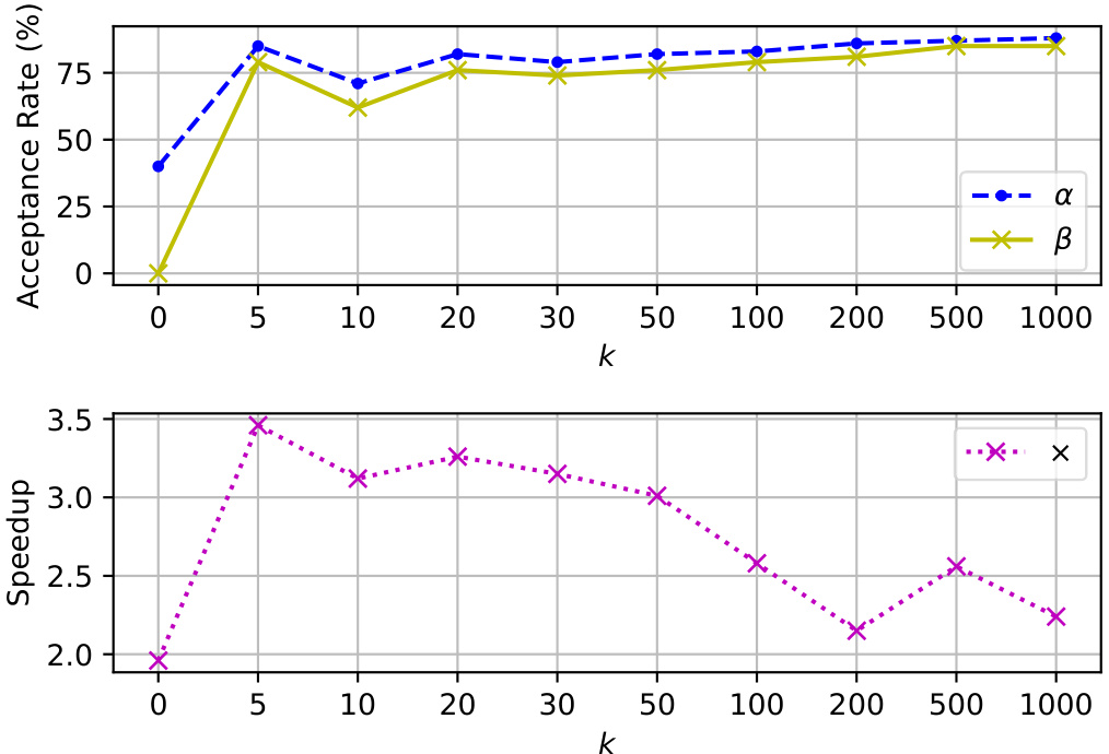
Figure 4. Upper: The acceptance rate $\alpha$ and $n$ -gram acceptance rate $\beta$ versus varying $k$ . Lower: The speedup $\times$ versus varying $k$
图 4: 上:接受率 $\alpha$ 和 $n$ -gram 接受率 $\beta$ 随 $k$ 变化的情况。下:加速比 $\times$ 随 $k$ 变化的情况。
Table 7. Acceptance rate α $\left(k=0\right)$ ) and speedup $\times$ across different tree configurations. Each configuration is represented by a 4-digit array: they represent the number of candidates for different decoding heads in §3.2.
表 7: 不同树配置下的接受率 α($\left(k=0\right)$)和加速比 $\times$。每个配置由一个 4 位数数组表示:它们代表第 3.2 节中不同解码头的候选数量。
Table 8. Distinct-n score across different penalty value θ. 1.0 indicate that no penalty is applied. We take $W=1024$ (See Appendix F.3 for ablation on $W$ ).
表 8: 不同惩罚值 θ 下的 Distinct-n 分数。1.0 表示未应用惩罚。我们取 $W=1024$(关于 $W$ 的消融实验见附录 F.3)。
| Gen.Len. | [3,3,3,3] | [1,9,9,9] | [1,3,3,3] (Ours) | |
|---|---|---|---|---|
| 20K | α | 0.44 | 0.50 | 0.45 |
| x(>1) | 1.34 | 0.53 | 1.56 | |
| 40K | α | 0.43 | 0.52 | 0.43 |
| x(>1) | 1.58 | 0.67 | 1.75 | |
| 60K | α | 0.43 | 0.53 | 0.42 |
| x(>1) | 1.75 | 0.78 | 1.88 | |
| 80K | α | 0.43 | 0.55 | 0.42 |
| x(>1) | 1.85 | 0.88 | 1.97 | |
| 100K | α | 0.42 | 0.57 | 0.40 |
| x(>1) | 1.91 | 0.96 | 1.96 |
| Distinct-1 | Distinct-2 | Distinct-3 | Distinct-4 | AVG. | |
|---|---|---|---|---|---|
| 1.0 | 0.07 | 0.11 | 0.14 | 0.15 | 0.12 |
| 1.1 | 0.08 | 0.13 | 0.15 | 0.16 | 0.13 |
| 1.2 | 0.41 | 0.71 | 0.81 | 0.82 | 0.69 |
| 1.3 | 0.57 | 0.86 | 0.93 | 0.95 | 0.83 |
| 1.4 | 0.52 | 0.73 | 0.76 | 0.77 | 0.70 |
| 1.5 | 0.74 | 0.96 | 0.98 | 0.99 | 0.92 |
4.4. Discussions
4.4. 讨论
In this section, we explore the effects of different hyper parameters on TOKENSWIFT.
在本节中,我们探讨了不同超参数对 TOKENSWIFT 的影响。
4.4.1. TREE CONFIGURATION
4.4.1. 树配置
Due to the time-consuming nature of finding the optimal tree in Medusa (Cai et al., 2024) and its limited impact on accelerating ultra-long sequences generation, we employ a simple 3-ary tree in tree attention. See Appendix B for the tree structure.
由于在 Medusa (Cai et al., 2024) 中找到最优树的过程耗时且对加速超长序列生成的影响有限,我们在树注意力中采用了简单的三叉树。树结构详见附录 B。
As shown in Table 7, [1,9,9,9] has the highest acceptance rate but the lowest speedup. This is because more candidates increase the acceptance rate, but also increase the verification burden. Similarly, by comparing [1,3,3,3] and [3,3,3,3], we can find that the first head (i.e., the original head of target model) achieves relatively high prediction accuracy when using KV compression, so choosing the top-1 token as candidate is sufficient. To balance the trade-off of acceptance rate and verification efficiency, we adopt [1,3,3,3] as the configuration of TOKENSWIFT.
如表 7 所示,[1,9,9,9] 的接受率最高,但加速比最低。这是因为更多的候选会增加接受率,但也会增加验证负担。同样,通过比较 [1,3,3,3] 和 [3,3,3,3],我们可以发现,在使用 KV 压缩时,第一个头 (即目标模型的原始头) 实现了相对较高的预测准确率,因此选择 top-1 token 作为候选就足够了。为了平衡接受率和验证效率,我们采用 [1,3,3,3] 作为 TOKENSWIFT 的配置。
4.4.2. N-GRAM CANDIDATES
4.4.2. N-GRAM 候选集
As illustrated in Figure 4, increasing $k$ enhances the $n$ -gram acceptance rate $\beta$ due to a larger pool of $n$ -gram candidates. However, an excessive number of candidates can strain the verification process, leading to reduced speedup $\times$ .
如图 4 所示,随着 $k$ 的增加,由于 $n$-gram 候选池的扩大,$n$-gram 接受率 $\beta$ 得到提升。然而,过多的候选词会给验证过程带来压力,导致加速比 $\times$ 下降。
Interestingly, a lower $k$ does not always result in a lower $\beta$ . For instance, $k=5$ achieves a higher $\beta$ than $k=20$ , resulting in both a higher acceptance rate $\alpha$ and greater speedu $_p\times$ . However, at $k=5$ , the lack of diversity among the candidates leads to increased repetition, which in turn degrades the quality of generation.
有趣的是,较低的 $k$ 并不总是导致较低的 $\beta$。例如,$k=5$ 实现了比 $k=20$ 更高的 $\beta$,从而获得了更高的接受率 $\alpha$ 和更大的速度 $_{p}\times$。然而,在 $k=5$ 时,候选者之间缺乏多样性导致重复增加,进而降低了生成的质量。
4.4.3. PENALTY VALUE $\theta$
4.4.3. 惩罚值 $\theta$
As a key component of TOKENSWIFT, contextual penalty significantly reduces repetition in generated text. We examine the effect of two parameters present in contextual penalty, i.e. penalty value $\theta$ and penalty window $W$ .
作为 TOKENSWIFT 的关键组件,上下文惩罚显著减少了生成文本中的重复。我们研究了上下文惩罚中两个参数的影响,即惩罚值 $\theta$ 和惩罚窗口 $W$。
Table 8 presents the impact of introducing contextual penalty on diversity. Without any penalty $(\theta=0)$ ), the generated sequences exhibit severe repetition, with an average Distinct $n$ score of only 0.12. As the value of $\theta$ increases gradually to 1.2, the diversity improves significantly, highlighting the effectiveness of contextual penalty in enhancing the diversity of ultra-long sequence generation.
表 8 展示了引入上下文惩罚对多样性的影响。在没有惩罚 $(\theta=0)$ 的情况下,生成的序列表现出严重的重复,平均 Distinct $n$ 得分仅为 0.12。随着 $\theta$ 的值逐渐增加到 1.2,多样性显著提高,凸显了上下文惩罚在增强超长序列生成多样性方面的有效性。
4.4.4. CASE STUDY
4.4.4. 案例研究
Figure 5 presents a case study on the impact of the contextual penalty. Without the Contextual Penalty, repetitions appear at about 5K tokens, compared to 60K with the penalty applied. Additionally, generation without the penalty exhibits word-for-word repetition, whereas generation with the penalty primarily demonstrates semanticlevel repetition, highlighting its effectiveness in mitigating redundancy.
图 5: 上下文惩罚影响的案例研究。在不使用上下文惩罚的情况下,重复现象出现在大约 5K Token 处,而应用惩罚后则出现在 60K Token 处。此外,未应用惩罚的生成表现出逐字重复,而应用惩罚的生成则主要表现出语义层面的重复,凸显了其在减少冗余方面的有效性。
5. Related Works
- 相关工作
5.1. Speculative Decoding
5.1. 推测解码 (Speculative Decoding)
Recent advancements in speculative decoding have significantly accelerated large language model (LLM) inference through diverse methodologies. Speculative decoding (Leviathan et al., 2023; Chen et al., 2023) traditionally leverages smaller draft models to propose candidate tokens for verification by the target model. Early works like SpecTr (Sun et al., 2023) introduced optimal transport for multi-candidate selection, while SpecInfer (Miao et al., 2024) and Medusa (Cai et al., 2024) pioneered tree-based structures with tree-aware attention and multi-head decoding to enable parallel verification of multiple candidates. Subsequent innovations, such as Sequoia (Chen et al., 2024b) and EAGLE-2 (Li et al., 2024d), optimized tree construction using dynamic programming and reordering strategies, while Hydra (Ankner et al., 2024) and ReDrafter (Cheng et al., 2024) enhanced tree dependencies through sequential or recurrent heads. Hardware-aware optimization s, exemplified by SpecExec (Sv ir sch evski et al., 2024) and Triforce (Sun et al., 2024a), further improved efficiency by leveraging hierarchical KV caching and quantized inference.
推测解码 (Speculative Decoding) 领域的最新进展通过多种方法显著加速了大语言模型 (LLM) 的推理。传统推测解码 (Leviathan et al., 2023; Chen et al., 2023) 利用较小的草稿模型提出候选 Token,供目标模型验证。早期的研究如 SpecTr (Sun et al., 2023) 引入了最优传输用于多候选选择,而 SpecInfer (Miao et al., 2024) 和 Medusa (Cai et al., 2024) 则开创了基于树结构的树感知注意力和多头解码,实现了多个候选的并行验证。随后的创新,如 Sequoia (Chen et al., 2024b) 和 EAGLE-2 (Li et al., 2024d),通过动态规划和重排序策略优化了树构建,而 Hydra (Ankner et al., 2024) 和 ReDrafter (Cheng et al., 2024) 则通过顺序或循环头增强了树的依赖关系。硬件感知优化方法,如 SpecExec (Sv ir sch evski et al., 2024) 和 Triforce (Sun et al., 2024a),通过利用分层 KV 缓存和量化推理进一步提高了效率。
Self-speculative approaches eliminate the need for external draft models by exploiting internal model dynamics. Draft&Verify (Zhang et al., 2024) and LayerSkip (Elhoushi et al., 2024) utilized early-exit mechanisms and Bayesian optimization to skip layers adaptively, whereas Kangaroo (Liu et al., 2024b) integrated dual early exits with lightweight adapters. Sun et al. (2024b) and SpecDec $^{++}$ (Huang et al., 2024) introduced theoretical frameworks for block-level token acceptance and adaptive candidate lengths. Parallel decoding paradigms, such as PASS (Monea et al., 2023) and MTJD (Qin et al., 2024), employed look-ahead embeddings or joint probability modeling to generate multiple candidates in a single pass, while CLLMs (Kou et al., 2024) and Lookahead (Fu et al., 2024) reimagined auto regressive consistency through Jacobi decoding and n-gram candidate pools.
自推测方法通过利用内部模型动态,消除了对外部草案模型的需求。Draft&Verify (Zhang et al., 2024) 和 LayerSkip (Elhoushi et al., 2024) 利用了早退机制和贝叶斯优化来自适应地跳过层,而 Kangaroo (Liu et al., 2024b) 则将双重早退与轻量级适配器相结合。Sun et al. (2024b) 和 SpecDec $^{++}$ (Huang et al., 2024) 引入了块级 Token 接受和自适应候选长度的理论框架。并行解码范式,如 PASS (Monea et al., 2023) 和 MTJD (Qin et al., 2024),采用了前瞻嵌入或联合概率建模来在一次通过中生成多个候选,而 CLLMs (Kou et al., 2024) 和 Lookahead (Fu et al., 2024) 则通过 Jacobi 解码和 n-gram 候选池重新构想了自回归一致性。
Retrieval-augmented methods like REST (He et al., 2024), and NEST (Li et al., 2024b) integrated vector or phrase retrieval to draft context-aware tokens, often combining copy mechanisms with confidence-based attribution. Training-centric strategies, including TR-Jacobi (Wang et al., 2024a), enhanced parallel decoding capability via noisy training or self-distilled multi-head architectures. System-level optimization s such as PipeInfer (Butler et al., 2024) and Narasimhan et al. (2024) addressed s cal ability through asynchronous pipelines and latencyaware scheduling, while Goodput (Liu et al., 2024c) focused on dynamic resource allocation and nested model
REST (He et al., 2024) 和 NEST (Li et al., 2024b) 等检索增强方法通过向量或短语检索来生成上下文感知的Token,通常结合复制机制和基于置信度的归因。以训练为核心的策略,包括 TR-Jacobi (Wang et al., 2024a),通过噪声训练或自蒸馏多头架构增强了并行解码能力。系统级优化如 PipeInfer (Butler et al., 2024) 和 Narasimhan et al. (2024) 通过异步流水线和延迟感知调度解决了可扩展性问题,而 Goodput (Liu et al., 2024c) 则专注于动态资源分配和嵌套模型。

Figure 5. Case Study on LLaMA3.1-8b. Left: fragments of generated text without Contextual Penalty. Right: fragments of generated text with Contextual Penalty. The blue text is repetition part. See Appendix $_\mathrm{G}$ for more cases.
图 5: LLaMA3.1-8b 的案例研究。左:未使用上下文惩罚时生成的文本片段。右:使用上下文惩罚时生成的文本片段。蓝色文本为重复部分。更多案例请参见附录 $_\mathrm{G}$。
deployment.
部署
Approaches such as Triforce (Sun et al., 2024a) and MagicDec (Chen et al., 2024a) incorporate KV cache compression during the drafting phase. However, their applicability is limited to scenarios characterized by long prefixes and short outputs, making them unsuitable for ultra-long sequence generation tasks. In such tasks, which are the focus of our work, the need for efficient inference spans both extended input contexts and lengthy outputs, presenting challenges that existing methods fail to address.
Triforce (Sun et al., 2024a) 和 MagicDec (Chen et al., 2024a) 等方法在草稿阶段引入了 KV 缓存压缩。然而,它们的适用性仅限于具有长前缀和短输出的场景,因此不适用于超长序列生成任务。在我们的工作中,这些任务需要高效的推理来应对扩展的输入上下文和冗长的输出,而现有方法无法解决这些挑战。
5.2. Long Sequence Generation
5.2. 长序列生成
Recent advances in long sequence generation have focused on addressing the challenges of coherence, efficiency, and s cal ability in producing extended outputs. A pivotal contribution is the LongWriter (Bai et al., 2024) framework, which introduces a task decomposition strategy to generate texts exceeding 20,000 words. Complementing this, Temp-Lora (Wang et al., 2024b) proposes inference-time training with temporary Lora modules to dynamically adapt model parameters during generation, offering a scalable alternative to traditional
长序列生成的最新进展主要集中在解决生成长文本时的连贯性、效率和可扩展性挑战。LongWriter (Bai et al., 2024) 框架是一个关键贡献,它引入了一种任务分解策略,能够生成超过 20,000 词的文本。与此同时,Temp-Lora (Wang et al., 2024b) 提出了在推理时使用临时 Lora 模块进行训练的方法,以动态调整生成过程中的模型参数,为传统方法提供了一种可扩展的替代方案。
KV caching. Similarly, PLANET (Hu et al., 2022) leverages dynamic content planning with sentence-level bag-ofwords objectives to improve logical coherence in opinion articles and argumentative essays, demonstrating the effectiveness of structured planning in auto regressive transformers.
KV 缓存。同样,PLANET (Hu et al., 2022) 利用动态内容规划与句子级别的词袋目标来提高意见文章和议论文的逻辑一致性,展示了结构化规划在自回归 Transformer 中的有效性。
In addition, lightweight decoding-side sampling strategies have emerged for repetition mitigation. The foundational work on Nucleus Sampling (Holtzman et al., 2020) first demonstrated that dynamically truncating low-probability token sets could reduce repetitive outputs while maintaining tractable decoding latency. Building on this, Hewitt et al. (2022) introduced $\eta$ -sampling explicitly linking candidate set reduction to repetition mitigation by entropy-guided token pruning. Recent variants like Min-p (Nguyen et al., 2024) optimize truncation rules in real-time—scaling thresholds to the maximum token probability. And Mirostat Sampling (Basu et al., 2021) further integrate lightweight Bayesian controllers to adjust $\eta$ parameters on-the-fly. Our work systematically analyzing how parameterized sampling (e.g., Top-p Min-p, $\eta$ -sampling) balances computational overhead and repetition suppression in ultra-long sequence generation pipelines.
此外,轻量级的解码端采样策略已经出现,用于缓解重复问题。Nucleus Sampling (Holtzman et al., 2020) 的基础工作首次证明了动态截断低概率Token集可以在保持可解码延迟的同时减少重复输出。在此基础上,Hewitt et al. (2022) 引入了 $\eta$ -采样,通过熵引导的Token剪枝明确将候选集缩减与重复缓解联系起来。最近的变体如 Min-p (Nguyen et al., 2024) 实时优化截断规则——将阈值缩放到最大Token概率。而 Mirostat Sampling (Basu et al., 2021) 进一步集成了轻量级贝叶斯控制器,以动态调整 $\eta$ 参数。我们的工作系统地分析了参数化采样(例如 Top-p Min-p, $\eta$ -采样)如何在超长序列生成管道中平衡计算开销和重复抑制。
6. Conclusion
6. 结论
In this study, we introduce TOKENSWIFT, a novel framework designed to achieve lossless acceleration in generating ultra-long sequences with LLMs. By analyzing and addressing three challenges, TOKENSWIFT significantly enhances the efficiency of the generation process. Our experimental results demonstrate that TOKENSWIFT achieves over $3\times$ acceleration across various model scales and architectures. Furthermore, TOKENSWIFT effectively mitigates issues related to repetitive content, ensuring the quality and coherence of the generated sequences. These advancements position TOKENSWIFT as a scalable and effective solution for ultra-long sequence generation tasks.
在本研究中,我们介绍了 TOKENSWIFT,这是一个旨在通过大语言模型实现超长序列无损加速生成的新框架。通过分析和解决三个挑战,TOKENSWIFT 显著提高了生成过程的效率。我们的实验结果表明,TOKENSWIFT 在各种模型规模和架构上实现了超过 $3\times$ 的加速。此外,TOKENSWIFT 有效缓解了与重复内容相关的问题,确保了生成序列的质量和连贯性。这些进展使 TOKENSWIFT 成为超长序列生成任务中可扩展且有效的解决方案。
Acknowledgements
致谢
We thank Haoyi Wu from Shanghai Tech University, Xuekai Zhu from Shanghai Jiaotong University, Hengli Li from Peking University for helpful discussions on speculative decoding and language modeling. This work presented herein is supported by the National Natural Science Foundation of China (62376031).
我们感谢上海科技大学的Haoyi Wu、上海交通大学的Xuekai Zhu和北京大学的Hengli Li在推测解码和语言建模方面的有益讨论。本文工作得到了国家自然科学基金(62376031)的支持。
References
参考文献
Qin, Z., Hu, Z., He, Z., Prakriya, N., Cong, J., and Sun, Y. Optimized multi-token joint decoding with auxiliary model for llm inference. arXiv preprint arXiv:2407.09722, 2024.
Qin, Z., Hu, Z., He, Z., Prakriya, N., Cong, J., 和 Sun, Y. 大语言模型推理中基于辅助模型的优化多Token联合解码。arXiv 预印本 arXiv:2407.09722, 2024.
Yuan, Z., Shang, Y., Zhou, Y., Dong, Z., Zhou, Z., Xue, C., Wu, B., Li, Z., Gu, Q., Lee, Y. J., et al. Llm inference unveiled: Survey and roofline model insights. arXiv preprint arXiv:2402.16363, 2024. Zhang, J., Wang, J., Li, H., Shou, L., Chen, K., Chen, G., and Mehrotra, S. Draft& verify: Lossless large language model acceleration via self-speculative decoding. In Ku, L.-W., Martins, A., and Srikumar, V. (eds.), Proceedings of the 62nd Annual Meeting of the Association for Computational Linguistics (Volume 1: Long Papers), pp. 11263– 11282, Bangkok, Thailand, August 2024. Association for Computational Linguistics. doi: 10.18653/v1/2024.acl -long.607. URL https://a cl anthology.org/2024.acl-long.607/.
Yuan, Z., Shang, Y., Zhou, Y., Dong, Z., Zhou, Z., Xue, C., Wu, B., Li, Z., Gu, Q., Lee, Y. J., et al. Llm inference unveiled: Survey and roofline model insights. arXiv preprint arXiv:2402.16363, 2024. Zhang, J., Wang, J., Li, H., Shou, L., Chen, K., Chen, G., and Mehrotra, S. Draft& verify: Lossless large language model acceleration via self-speculative decoding. In Ku, L.-W., Martins, A., and Srikumar, V. (eds.), Proceedings of the 62nd Annual Meeting of the Association for Computational Linguistics (Volume 1: Long Papers), pp. 11263– 11282, Bangkok, Thailand, August 2024. Association for Computational Linguistics. doi: 10.18653/v1/2024.acl -long.607. URL https://a cl anthology.org/2024.acl-long.607/.
A. Lossless Nature of Speculative Decoding
A. 推测解码的无损性质
The speculative decoding (Leviathan et al., 2023; Chen et al., 2023) can easily be justified to be lossless and identical to sample from $q_{t a r g e t}$ alone, i.e., $p_{S D}=q_{t a r g e t}$ . Note that, given prefix $X_{1:j},$ the next token sampled from:
推测解码 (Leviathan et al., 2023; Chen et al., 2023) 可以很容易地证明是无损的,并且与单独从 $q_{t a r g e t}$ 采样相同,即 $p_{S D}=q_{t a r g e t}$。请注意,给定前缀 $X_{1:j},$ 下一个 Token 的采样来源为:

where $\alpha$ is the acceptance rate given by
其中 $\alpha$ 为接受率,其表达式为

If the draft token is accepted, we have
如果草稿Token被接受,我们有

If the token is rejected, we have
如果Token被拒绝,我们

Therefore, the overall probability is given by
因此,整体概率为

Proved.
证明。
B. Additional Training and Inference Details.
B. 额外的训练和推理细节
B.1. Training Details
B.1. 训练细节
During training, only three linear layers are fine-tuned, while the parameters of the LLM remained fixed. The model was trained on an NVIDIA A100-SXM4-80GB GPU. The specific training parameters are outlined in Table 9.
在训练过程中,仅微调了三个线性层,而大语言模型的参数保持不变。模型在 NVIDIA A100-SXM4-80GB GPU 上进行训练。具体的训练参数如表 9 所示。
Table 9. Additional training details. Note that these hyper parameters do not require extensive tuning.
表 9: 额外训练细节。请注意,这些超参数不需要大量调优。
| LLaMA3.1-8b | YaRN-LLaMA2-7b-128k | Qwen2.5-1.5b | Qwen2.5-7b | Qwen2.5-14b | |
|---|---|---|---|---|---|
| optimizer | AdamW | AdamW | AdamW | AdamW | AdamW |
| betas | (0.9, 0.999) | (0.9, 0.999) | (0.9, 0.999) | (0.9, 0.999) | (0.9, 0.999) |
| weight decay | 0.1 | 0.1 | 0.1 | 0.1 | 0.1 |
| warmup steps | 50 | 50 | 50 | 50 | 50 |
| learning rate scheduler | cosine | cosine | cosine | cosine | cosine |
| num. GPUs | 4 | 4 | 4 | 4 | 4 |
| gradient accumulation steps | 10 | 10 | 10 | 10 | 10 |
| batch size per GPU | 3 | 3 | 3 | 3 | 3 |
| num. steps | 200 | 200 | 200 | 200 | 200 |
| learning rate | 5e-3 | 5e-3 | 5e-3 | 5e-3 | 5e-3 |
Table 10. k stands for the maximum number of retrieved $\mathbf{n}$ -grams in token re utilization
表 10: k 表示 Token 重复利用中检索到的 $\mathbf{n}$ -gram 的最大数量
| k | temp. | top-p | min-p | penalty | penalty len. | |
|---|---|---|---|---|---|---|
| LLaMA3.1-8b | 1.0 | 0.1 | 1.2 | 1024 | ||
| YaRN-LLaMA2-7b-128k | 1.0 | 0.9 | 1.15 | 1024 | ||
| Qwen2.5-1.5b | 1.0 | 0.9 | 1.15 | 1024 | ||
| Qwen2.5-7b | 1.0 | 0.05 | 1.15 | 1024 | ||
| Qwen2.5-14b | 1.0 | 0.05 | 1.13 | 1024 |
B.2. Inference Details
B.2. 推理细节
For inference, we used 4-grams to maintain consistency with multi-token generation. The specific inference parameters are presented in Table 10.
在推理过程中,我们使用了4-gram以保持与多Token生成的一致性。具体的推理参数如表 10 所示。
For the tree attention mechanism, we selected a simple ternary full tree configuration, as depicted in Appendix B.2.
对于树注意力机制,我们选择了一种简单的三元满树配置,如附录 B.2 所示。

C. Pre-training Details of the Llama3.1 Draft Model
C. Llama3.1 草稿模型的预训练细节
To serve as the draft model for LLaMA3.1-8b in TriForce, we pretrain a tiny version of 250M parameters with the same tokenizer from LLaMA3.1-8b. The model configuration is listed in Table 11. We train the model on Wikipedia (20231101.en) 5 and part of $\mathrm{C}4\mathrm{-en}^{6}$ for 1 epoch.
作为 TriForce 中 LLaMA3-8b 的草稿模型,我们使用与 LLaMA3-8b 相同的 Tokenizer 预训练了一个包含 2.5 亿参数的迷你版本。模型配置如表 11 所示。我们在 Wikipedia (20231101.en) 和部分 $\mathrm{C}4\mathrm{-en}^{6}$ 上训练该模型 1 个 epoch。
Table 11. Configuration of Llama 3.1 205M.
表 11: Llama 3.1 205M 的配置
| hidden_size | 768 |
|---|---|
| hidden-act | silu |
| intermediate_size | 3072 |
| max-position_embeddings | 2048 |
| num_attention_heads | 12 |
| num_key-value_heads | 12 |
| rope_theta | 500000 |
| vocab_size | 128256 |
D. Different Sampling Method
D. 不同采样方法
D.1. Introduction of Different Sampling Algorithms
D.1. 不同采样算法的介绍
Given a probability distribution $P(x_{t}|x_{1},x_{2},\ldots,x_{t-1})$ over the vocabulary $\nu$ at position $t,$ top $p$ sampling (Holtzman et al., 2020) first sorts the tokens in descending order of their probabilities. It then selects the smallest set of tokens whose cumulative probability exceeds a predefined threshold $p$ , where $p\in(0,1]$ . Formally, let $\mathcal{V}_{p}\subset\mathcal{V}$ be the smallest set such that:
给定位置 $t$ 处词汇表 $\nu$ 上的概率分布 $P(x_{t}|x_{1},x_{2},\ldots,x_{t-1})$,top $p$ 采样 (Holtzman et al., 2020) 首先按照概率降序对 token 进行排序。然后选择累积概率超过预定义阈值 $p$ 的最小 token 集,其中 $p\in(0,1]$。形式上,设 $\mathcal{V}_{p}\subset\mathcal{V}$ 为满足以下条件的最小集合:

The next token $\hat{x_{t}}$ is then randomly sampled from this reduced set $\mathcal{V}_{p}$ according to the re normalized probabilities:
下一个 Token $\hat{x_{t}}$ 随后根据重新归一化的概率从缩减后的集合 $\mathcal{V}_{p}$ 中随机采样:

Nguyen et al. (2024) introduced min-p sampling, which uses a relative probability threshold $p_{b a s e}\in(0,1]$ to scale the maximum token probability $p_{m a x}$ to determine the absolute probability threshold $p_{s c a l e d}$ . Sampling is then performed on tokens with probability greater than or equal to $p_{s c a l e d}$ .
Nguyen 等人 (2024) 提出了最小概率采样 (min-p sampling),该方法使用相对概率阈值 $p_{b a s e}\in(0,1]$ 来缩放最大 Token 概率 $p_{m a x}$,从而确定绝对概率阈值 $p_{s c a l e d}$。然后对概率大于或等于 $p_{s c a l e d}$ 的 Token 进行采样。
Formally, given the maximum probability over the token distribution $p_{m a x}=\operatorname*{max}{v\in\mathcal{V}}P\big(x{t}=v|x_{1},x_{2},\dots,x_{t-1}\big),$ the absolute probability threshold $p_{s c a l e d}$ is calculated as:
形式上,给定Token分布的最大概率 $p_{m a x}=\operatorname*{max}{v\in\mathcal{V}}P\big(x{t}=v|x_{1},x_{2},\dots,x_{t-1}\big),$ 绝对概率阈值 $p_{s c a l e d}$ 的计算公式为:

The sampling pool $\nu_{m i n}$ is then defined as the set of tokens whose probability is greater than or equal to $p_{s c a l e d}$
采样池 $\nu_{m i n}$ 随后被定义为概率大于或等于 $p_{s c a l e d}$ 的 Token 集合

Finally, the next token ${\hat{x}}{t}$ is randomly sampled from the set $\nu{m i n}$ according to the normalized probabilities:
最后,根据归一化概率从集合 $\nu_{m i n}$ 中随机采样下一个 Token ${\hat{x}}_{t}$:

The sampling pool of $\eta$ -sampling (Hewitt et al., 2022) is defined as
$\eta$ 采样的采样池 (Hewitt et al., 2022) 定义为

where $h_{\theta,x_{<i}}$ is the entropy of $P(\mathcal{V}|x_{1},x_{2},...,x_{t-1})$ , $\alpha$ and $\epsilon$ are hyper parameters.
其中 $h_{\theta,x_{<i}}$ 是 $P(\mathcal{V}|x_{1},x_{2},...,x_{t-1})$ 的熵,$\alpha$ 和 $\epsilon$ 是超参数。
D.2. Impact of Different Sampling Algorithms
D.2. 不同采样算法的影响
We also explored the impact of different sampling algorithms with disable token re utilization, including top $p$ sampling (Holtzman et al., 2020), min $p$ sampling (Nguyen et al., 2024), and $\eta$ -sampling (Hewitt et al., 2022). As summarized in Table 12, TOKENSWIFT consistently demonstrates strong robustness across these methods. This versatility underscores its compatibility with a wide range of decoding strategies, making it suitable for diverse applications and use cases.
我们还探索了禁用Token重复利用的不同采样算法的影响,包括top $p$采样 (Holtzman et al., 2020)、min $p$采样 (Nguyen et al., 2024) 和 $\eta$-采样 (Hewitt et al., 2022)。如表12总结所示,TOKENSWIFT在这些方法中始终表现出强大的鲁棒性。这种多功能性凸显了其与多种解码策略的兼容性,使其适用于各种应用和用例。
E. Tree-Based Attention
E. 基于树的注意力机制 (Tree-Based Attention)
Tree attention is a mechanism designed to process multiple candidate continuations during speculative decoding efficiently. Instead of selecting a single continuation as in traditional methods, tree attention leverages multiple candidates to increase the expected acceptance length in each decoding step, balancing computational demands and performance.
树注意力机制是一种旨在推测解码过程中高效处理多个候选延续的机制。与传统方法中选择单一延续不同,树注意力机制利用多个候选延续来增加每个解码步骤中的预期接受长度,从而在计算需求和性能之间取得平衡。
Table 12. Ablation results on various sampling methods with disable token re utilization.
表 12. 禁用 Token 重用的各种采样方法的消融结果
| Gen. Len. | top-p (p = 0.9) | min-p (p = 0.1) | r-sampling (e =2e-4) | |
|---|---|---|---|---|
| 20K | α | 0.68 | 0.66 | 0.56 |
| x(>1) | 2.10 | 2.01 | 1.85 | |
| 40K | & | 0.81 | 0.75 | 0.71 |
| x(>1) | 2.80 | 2.58 | 2.59 | |
| 60K | 0.84 | 0.79 | 0.78 | |
| x(>1) | 3.07 | 2.94 | 2.99 | |
| 80K | 0.86 | 0.81 | 0.81 | |
| x(>1) | 3.28 | 3.15 | 3.24 | |
| 100K | α | 0.87 | 0.82 | 0.84 |
| x(>1) | 3.42 | 3.26 | 3.42 |
The mechanism uses a tree structure where each branch represents a unique candidate continuation. For example, if two heads generate top-2 and top-3 predictions, the Cartesian product of these predictions results in 6 candidates, forming a tree with 6 branches. Each token in the tree attends only to its predecessors, and an attention mask ensures that this constraint is upheld. Positional indices are also adjusted to align with the tree structure.
该机制采用树结构,其中每个分支代表一个独特的候选延续。例如,如果两个头生成前2和前3的预测,这些预测的笛卡尔积会产生6个候选,形成具有6个分支的树。树中的每个 Token 仅关注其前驱,并且注意力掩码确保这一约束得到维护。位置索引也会进行调整以与树结构对齐。
The tree structure is constructed by taking the Cartesian product of the predictions across all heads. If head $k$ has $s_{k}$ top predictions, then the tree structure consists of all possible combinations of predictions across the heads. Each combination forms a unique branch in the tree.
树结构是通过在所有头部的预测之间进行笛卡尔积构建的。如果头部 $k$ 有 $s_{k}$ 个顶级预测,那么树结构由所有头部预测的可能组合组成。每个组合在树中形成一个唯一的分支。
Let the total number of candidates (i.e., branches) in the tree be denoted as $C$ , which is the product of the number of predictions for each head:
设树中的候选总数(即分支)为 $C$,它是每个头预测数的乘积:

Each candidate is a distinct sequence of tokens formed by selecting one token from each set of predictions from the heads.
每个候选者都是从各个头部的预测集合中选择一个Token形成的独特Token序列。
To ensure that tokens only attend to their predecessors (tokens generated earlier in the continuation), an attention mask is applied. The attention mask for the tree structure ensures that for each token at level $k_{\rightmoon}$ , it can attend only to tokens in levels ${0,1,\ldots,k-1}$ . This guarantees that each token’s attention is directed solely towards its predecessors in the tree.
为确保 Token 仅关注其前驱(即续写过程中较早生成的 Token),应用了注意力掩码。树结构中的注意力掩码确保对于层级 $k_{\rightmoon}$ 上的每个 Token,它只能关注层级 ${0,1,\ldots,k-1}$ 中的 Token。这保证了每个 Token 的注意力仅指向其在树中的前驱。
Formally, the attention mask $M_{k}$ for each token at level $k$ is defined as:
形式上,每个在层级 $k$ 的 Token 的注意力掩码 $M_{k}$ 定义为:

where $M_{k}(i,j)=1$ means that the token at position $j$ can attend to the token at position $i,$ and $M_{k}(i,j)=0$ means no attention is allowed from $j$ to $i$ .
其中 $M_{k}(i,j)=1$ 表示位置 $j$ 的 Token 可以关注位置 $i$ 的 Token,而 $M_{k}(i,j)=0$ 表示不允许从 $j$ 到 $i$ 的关注。
F. More Ablation Experiments
F. 更多消融实验
F.1. Ablation of Temperature
F.1. 温度消融实验
Table 13 presents the results of an ablation experiment investigating the effect of varying temperature settings on the generation length, acceptance rate, and speedup during text generation. The experiment uses top $p$ sampling with a fixed $p$ of 0.9 and evaluates generation lengths ranging from 20K to 100K tokens, with temperature values spanning from 0.4 to 1.2.
表 13 展示了一项消融实验的结果,该实验研究了不同温度设置对文本生成过程中生成长度、接受率和加速比的影响。实验使用 top $p$ 采样,固定 $p$ 为 0.9,并评估了从 20K 到 100K token 的生成长度,温度值范围从 0.4 到 1.2。
From the results, it is evident that as temperature increases, acceptance rate generally decreases across all generation lengths. Specifically, acceptance rate drops from 0.79 at a temperature of 0.4 to 0.52 at a temperature of 1.2 for 20K-length generation, and a similar trend is observed for longer sequences. This suggests that higher temperatures result in more diverse but less accurate output. On the other hand, speedup tends to remain relatively stable or slightly decrease with higher temperatures. The highest speedups, reaching around 3.4, are observed across all generation lengths with temperatures around 0.6 and 1.0, indicating that moderate temperature settings offer the best balance between speed and quality.
从结果中可以明显看出,随着温度的增加,所有生成长度的接受率普遍下降。具体来说,对于20K长度的生成,接受率从温度为0.4时的0.79下降到温度为1.2时的0.52,对于更长的序列也观察到了类似的趋势。这表明较高的温度会导致输出更加多样化但准确性降低。另一方面,随着温度的升高,加速比往往保持相对稳定或略有下降。在所有生成长度中,温度在0.6和1.0左右时观察到最高的加速比,达到约3.4,这表明适中的温度设置在速度和质量之间提供了最佳平衡。
Table 13. Ablation results on varying temperatures. Using top $p$ sampling, with $p$ set to 0.9.
表 13. 不同温度下的消融实验结果。使用 top $p$ 采样,$p$ 设置为 0.9。
| Gen. Len. | 0.4 | 0.6 | 0.8 | 1.0 | 1.2 |
|---|---|---|---|---|---|
| 20K | & x(>1) | 0.79 0.84 2.25 2.34 | 0.56 1.80 | 0.68 2.10 | 0.52 1.72 |
| 40K | & x(> 1) | 0.85 2.76 | 0.88 2.80 | 0.73 0.81 2.60 2.80 | 0.69 2.52 |
| 60K | & x(>1) | 0.87 3.07 | 0.89 3.10 | 0.80 0.84 3.05 3.07 | 0.77 2.96 |
| 80K | & x(> 1) | 0.88 3.26 | 0.90 3.29 | 0.83 3.29 3.28 | 0.86 0.81 3.22 |
| 100K | & x(> 1) | 0.89 3.39 | 0.90 3.41 | 0.85 0.87 3.45 3.42 | 0.83 3.42 |
F.2. Ablation of Prefill Length
F.2. 预填充长度消融实验
We disable token re utilization and conduct ablation study on the different prefix length, as shown in Table 14. The experiment explores the impact of varying prefix lengths on the generation of sequences of different lengths (from 20K to 100K). The results include two key metrics: acceptance rate $(\alpha)$ and speedup factor $(\times)$ .
我们禁用 Token 重用,并对不同前缀长度进行消融研究,如表 14 所示。实验探讨了不同前缀长度对生成不同长度序列(从 20K 到 100K)的影响。结果包括两个关键指标:接受率 $(\alpha)$ 和加速因子 $(\times)$。
As the prefix length increases, the acceptance rate tends to stabilize, generally hovering around 0.35 to 0.39 across different sequence lengths, with a slight fluctuation depending on the specific prefix length. This suggests that while the acceptance rate does not dramatically change with longer sequences, it remains relatively consistent.
随着前缀长度的增加,接受率趋于稳定,通常在不同序列长度下保持在 0.35 到 0.39 之间,具体前缀长度的不同会带来轻微波动。这表明虽然接受率不会随着序列长度的增加而显著变化,但仍保持相对一致。
Table 14. Ablation results on different prefill length disable token re utilization.
表 14: 不同预填充长度下禁用Token重用的消融实验结果
| PrefillLen. | 20K | 20K | 40K | 40K | 60K | 60K | 80K | 80K | 100K | 100K |
|---|---|---|---|---|---|---|---|---|---|---|
| X | X | & | X | X | ||||||
| 2048 | 0.35 | 1.41 | 0.35 | 1.63 | 0.35 | 1.76 | 0.35 | 1.83 | 0.34 | 1.87 |
| 3072 | 0.31 | 1.23 | 0.31 | 1.42 | 0.31 | 1.55 | 0.31 | 1.64 | 0.30 | 1.69 |
| 4096 | 0.35 | 1.32 | 0.35 | 1.54 | 0.35 | 1.69 | 0.35 | 1.76 | 0.35 | 1.85 |
| 5120 | 0.32 | 1.29 | 0.31 | 1.46 | 0.31 | 1.57 | 0.31 | 1.65 | 0.31 | 1.70 |
| 6144 | 0.39 | 1.46 | 0.39 | 1.66 | 0.39 | 1.80 | 0.39 | 1.88 | 0.39 | 1.94 |
| 7168 | 0.36 | 1.42 | 0.37 | 1.62 | 0.36 | 1.74 | 0.36 | 1.82 | 0.36 | 1.88 |
| 8192 | 0.36 | 1.21 | 0.36 | 1.42 | 0.36 | 1.58 | 0.36 | 1.69 | 0.36 | 1.77 |
In terms of speedup, it shows that with longer prefix lengths, the model achieves progressively higher acceleration. For instance, a prefix length of 2048 achieves a speedup of 1.41 for 20K tokens, but with 8192, the speedup reaches up to 1.77 for 100K tokens. This indicates that increasing the prefix length contributes to better acceleration, especially for longer sequences, while maintaining a relatively stable acceptance rate. The findings demonstrate the tradeoff between prefix length and model efficiency, where larger prefix lengths tend to result in greater speed.
在加速方面,随着前缀长度的增加,模型实现了逐步更高的加速。例如,前缀长度为 2048 时,对于 20K Token 的加速比为 1.41,而当前缀长度为 8192 时,对于 100K Token 的加速比可达到 1.77。这表明增加前缀长度有助于实现更好的加速效果,尤其是在处理较长序列时,同时保持相对稳定的接受率。这些发现展示了前缀长度与模型效率之间的权衡,较大的前缀长度往往能带来更大的加速效果。
F.3. Ablation of Penalty Window
F.3. 惩罚窗口的消融实验
We investigate the effect of penalty window size $(W)$ on the performance of a model generating sequences of varying lengths (from 20K to 100K tokens). For each sequence length, we apply a penalty to generated tokens within a sliding window of size $W.$ , and evaluate the impact on two key metrics: acceptance rate $(\alpha)$ and acceleration factor $(\times)$ . Additionally, we assess the diversity of the generated sequences using the Distinct $n$ metric, where higher values indicate greater diversity.
我们研究了惩罚窗口大小 $(W)$ 对生成不同长度序列(从 20K 到 100K Token)模型性能的影响。对于每个序列长度,我们在大小为 $W$ 的滑动窗口内对生成的 Token 施加惩罚,并评估其对两个关键指标的影响:接受率 $(\alpha)$ 和加速因子 $(\times)$ 。此外,我们使用 Distinct $n$ 指标评估生成序列的多样性,其中较高的值表示更大的多样性。
Table 15. Ablation results on penalty length (W).
表 15: 惩罚长度 (W) 的消融结果
| 惩罚长度 (W) | 20K | 40K | 60K | 80K | 100K |
|---|---|---|---|---|---|
| α | X | ||||
| 20 | 0.82 | 2.25 | 0.90 | 2.85 | 0.93 |
| 50 | 0.83 | 2.30 | 0.89 | 2.83 | 0.91 |
| 128 | 0.59 | 1.75 | 0.70 | 2.38 | 0.75 |
| 256 | 0.78 | 2.17 | 0.86 | 2.76 | 0.89 |
| 512 | 0.75 | 2.15 | 0.84 | 2.73 | 0.88 |
| 1024 | 0.66 | 2.01 | 0.75 | 2.58 | 0.79 |
| 2048 | 0.69 | 1.99 | 0.79 | 2.58 | 0.82 |
Table 16. Distinct $^n$ score with different penalty length W.
表 16: 不同惩罚长度 W 下的 Distinct $^n$ 得分
| 惩罚长度 (W) | Distinct-1 | Distinct-2 | Distinct-3 | Distinct-4 | 平均值 |
|---|---|---|---|---|---|
| 20 | 0.85 | 0.86 | 0.73 | 0.70 | 0.79 |
| 50 | 0.91 | 0.91 | 0.85 | 0.77 | 0.86 |
| 128 | 0.95 | 0.77 | 0.57 | 0.48 | 0.69 |
| 256 | 0.83 | 0.91 | 0.88 | 0.83 | 0.86 |
| 512 | 0.90 | 0.86 | 0.74 | 0.65 | 0.79 |
| 1024 | 0.79 | 0.86 | 0.77 | 0.71 | 0.78 |
| 2048 | 0.67 | 0.84 | 0.86 | 0.84 | 0.80 |
The results in Table 15 and Table 16 show a clear trade-off between the penalty window size and the model’s performance. For smaller penalty window sizes, such as $W=20$ , the model achieves higher acceptance rates and better acceleration, but this comes at the cost of lower diversity in the generated sequences (as indicated by lower Distinct-n values). As the penalty window size increases (e.g., $W=256$ or $W=2048^{\cdot}$ ), the acceptance rate slightly decreases, but the model exhibits better diversity and still maintains a significant speedup relative to the AR baseline. These findings suggest that larger penalty windows can help reduce repetitive ness and improve the diversity of long sequence generation, but they may also slightly reduce the model’s efficiency and acceptance rate.
表 15 和表 16 中的结果显示,惩罚窗口大小和模型性能之间存在明显的权衡关系。对于较小的惩罚窗口大小(如 $W=20$),模型实现了更高的接受率和更好的加速效果,但这是以生成序列的多样性降低为代价的(如较低的 Distinct-n 值所示)。随着惩罚窗口大小的增加(例如 $W=256$ 或 $W=2048^{\cdot}$),接受率略有下降,但模型表现出更好的多样性,并且相对于自回归 (AR) 基线仍然保持了显著的加速。这些发现表明,较大的惩罚窗口有助于减少重复性并提高长序列生成的多样性,但也可能略微降低模型的效率和接受率。
Table 15 also reveals that for each penalty window size, increasing the sequence length (from 20K to 100K tokens) generally results in higher acceleration and better diversity, with some fluctuations in acceptance rates.
表 15 还显示,对于每个惩罚窗口大小,增加序列长度(从 20K 到 100K Token)通常会带来更高的加速和更好的多样性,但接受率会出现一些波动。
G. More Cases H. Training Loss Curve
G. 更多案例 H. 训练损失曲线

Figure 6. Case Study on YaRN-LLaMA2-7b-128k. Left: fragments of generated text without Contextual Penalty. Right: fragments of generated text with Contextual Penalty. The blue text is repetition part.
图 6: YaRN-LLaMA2-7b-128k 的案例研究。左:未使用上下文惩罚生成的文本片段。右:使用上下文惩罚生成的文本片段。蓝色文本为重复部分。


train/ce_loss_3 Figure 7. Cross Entropy Loss Training Curve of Linear Layers
图 7: 线性层的交叉熵损失训练曲线