Brain Tumor Segmentation with Deep Neural Networks\$
基于深度神经网络的脑肿瘤分割
Abstract
摘要
In this paper, we present a fully automatic brain tumor segmentation method based on Deep Neural Networks (DNNs). The proposed networks are tailored to glioblastoma s (both low and high grade) pictured in MR images. By their very nature, these tumors can appear anywhere in the brain and have almost any kind of shape, size, and contrast. These reasons motivate our exploration of a machine learning solution that exploits a flexible, high capacity DNN while being extremely efficient. Here, we give a description of different model choices that we’ve found to be necessary for obtaining competitive performance. We explore in particular different architectures based on Convolutional Neural Networks (CNN), i.e. DNNs specifically adapted to image data. We present a novel CNN architecture which differs from those traditionally used in computer vision. Our CNN exploits both local features as well as more global contextual features simultaneously. Also, different from most traditional uses of CNNs, our networks use a final layer that is a convolutional implementation of a fully connected layer which allows a 40 fold speed up. We also describe a 2-phase training procedure that allows us to tackle difficulties related to the imbalance of tumor labels. Finally, we explore a cascade architecture in which the output of a basic CNN is treated as an additional source of information for a subsequent CNN. Results reported on the 2013 BRATS test dataset reveal that our architecture improves over the currently published state-of-the-art while being over 30 times faster.
本文提出了一种基于深度神经网络 (DNN) 的全自动脑肿瘤分割方法。所提出的网络专门针对磁共振成像 (MRI) 中呈现的胶质母细胞瘤 (包括低级别和高级别) 进行优化。由于这类肿瘤可能出现在大脑任何位置,且形态、尺寸和对比度差异极大,这促使我们探索一种兼具灵活性与高效性的高容量DNN机器学习解决方案。我们详细阐述了为获得竞争优势而必须采用的不同模型选择策略,重点研究了基于卷积神经网络 (CNN) 的各种架构设计 (即专门适配图像数据的DNN)。我们提出了一种区别于传统计算机视觉应用的新型CNN架构,该网络能同步利用局部特征和全局上下文特征。与大多数传统CNN应用不同,我们的网络采用全连接层的卷积实现作为最终层,实现了40倍的速度提升。此外,我们描述了一种两阶段训练方案以解决肿瘤标签不平衡问题,并探索了级联架构——将基础CNN的输出作为后续CNN的附加信息源。在2013年BRATS测试数据集上的实验表明,该架构在超越当前最优性能的同时,处理速度提升超过30倍。
Keywords: Brain tumor segmentation, deep neural networks
关键词:脑肿瘤分割,深度神经网络
1. Introduction
1. 引言
In the United States alone, it is estimated that 23,000 new cases of brain cancer will be diagnosed in $2015^{2}$ . While gliomas are the most common brain tumors, they can be less aggressive (i.e. low grade) in a patient with a life expectancy of several years, or more aggressive (i.e. high grade) in a patient with a life expectancy of at most 2 years.
仅在美国,预计2015年将新增23,000例脑癌确诊病例$^{2}$。虽然胶质瘤是最常见的脑肿瘤,但患者的侵袭性可能较低(即低级别),预期寿命可达数年;也可能更具侵袭性(即高级别),预期寿命最多只有2年。
Although surgery is the most common treatment for brain tumors, radiation and chemotherapy may be used to slow the growth of tumors that cannot be physically removed. Magnetic resonance imaging (MRI) provides detailed images of the brain, and is one of the most common tests used to diagnose brain tumors. All the more, brain tumor segmentation from MR images can have great impact for improved diagnostics, growth rate prediction and treatment planning.
虽然手术是治疗脑肿瘤最常见的方法,但对于无法通过手术切除的肿瘤,可采用放疗和化疗来延缓其生长。磁共振成像 (MRI) 能提供脑部详细图像,是诊断脑肿瘤最常用的检测手段之一。更重要的是,基于MRI图像的脑肿瘤分割技术对提升诊断精度、预测生长速率及制定治疗方案具有重大意义。
While some tumors such as men ing iom as can be easily segmented, others like gliomas and glioblastoma s are much more difficult to localize. These tumors (together with their surrounding edema) are often diffused, poorly contrasted, and extend tentacle-like structures that make them difficult to segment. Another fundamental difficulty with segmenting brain tumors is that they can appear anywhere in the brain, in almost any shape and size. Furthermore, unlike images derived from X-ray computed tomography (CT) scans, the scale of voxel values in MR images is not standardized. Depending on the type of MR machine used (1.5, 3 or 7 tesla) and the acquisition protocol (field of view value, voxel resolution, gradient strength, b0 value, etc.), the same tumorous cells may end up having drastically different grayscale values when pictured in different hospitals.
虽然某些肿瘤(如脑膜瘤)易于分割,但胶质瘤和胶质母细胞瘤等肿瘤的定位则困难得多。这些肿瘤(连同周围水肿区)往往呈现弥散性、对比度低且具有触须状延伸结构,导致分割难度大。脑肿瘤分割的另一根本性挑战在于其可能出现在大脑任何位置,形态大小几乎无规律可循。此外,与X射线计算机断层扫描(CT)不同,磁共振成像(MR)的体素值范围缺乏统一标准。根据所用MR设备类型(1.5T、3T或7T)和采集协议(视野值、体素分辨率、梯度强度、b0值等),相同的肿瘤细胞在不同医院成像时可能呈现完全不同的灰度值。
Healthy brains are typically made of 3 types of tissues: the white matter, the gray matter, and the cerebrospinal fluid. The goal of brain tumor segmentation is to detect the location and extension of the tumor regions, namely active tumorous tissue (vascular i zed or not), necrotic tissue, and edema (swelling near the tumor). This is done by identifying abnormal areas when compared to normal tissue. Since glioblastoma s are infiltrative tumors, their borders are often fuzzy and hard to distinguish from healthy tissues. As a solution, more than one MRI modality is often employed, e.g. T1 (spin-lattice relaxation), T1-contrasted (T1C), T2 (spin-spin relaxation), proton density (PD) contrast imaging, diffusion MRI (dMRI), and fluid attenuation inversion recovery (FLAIR) pulse sequences. The contrast between these modalities gives almost a unique signature to each tissue type.
健康的大脑通常由三种组织构成:白质、灰质和脑脊液。脑肿瘤分割的目标是检测肿瘤区域的位置和范围,即活跃的肿瘤组织(无论是否血管化)、坏死组织以及水肿(肿瘤附近的肿胀)。这是通过与正常组织对比来识别异常区域实现的。由于胶质母细胞瘤具有浸润性,其边界通常模糊不清,难以与健康组织区分。为此,通常会采用多种MRI模态,例如T1(自旋-晶格弛豫)、T1增强(T1C)、T2(自旋-自旋弛豫)、质子密度(PD)对比成像、扩散MRI(dMRI)以及液体衰减反转恢复(FLAIR)脉冲序列。这些模态之间的对比几乎为每种组织类型提供了独特的特征。
Most automatic brain tumor segmentation methods use handdesigned features [15, 32]. These methods implement a classical machine learning pipeline according to which features are first extracted and then given to a classifier whose training procedure does not affect the nature of those features. An alternative approach for designing task-adapted feature representations is to learn a hierarchy of increasingly complex features directly from in-domain data. Deep neural networks have been shown to excel at learning such feature hierarchies [7]. In this work, we apply this approach to learn feature hierarchies adapted specifically to the task of brain tumor segmentation that combine information across MRI modalities.
大多数自动脑肿瘤分割方法使用手工设计的特征 [15, 32]。这些方法采用经典的机器学习流程:先提取特征,再将其输入分类器,而分类器的训练过程不会改变这些特征的本质。另一种设计任务自适应特征表示的方法是从领域数据中直接学习逐渐复杂的特征层次结构。深度神经网络已被证明擅长学习此类特征层次 [7]。在本研究中,我们应用这种方法来学习专门适应脑肿瘤分割任务的特征层次结构,这些结构能融合多模态MRI信息。
Specifically, we investigate several choices for training Convolutional Neural Networks (CNNs), which are Deep Neural Networks (DNNs) adapted to image data. We report their advantages, disadvantages and performance using well established metrics. Although CNNs first appeared over two decades ago [29], they have recently become a mainstay of the computer vision community due to their record-shattering performance in the ImageNet Large-Scale Visual Recognition Challenge [27]. While CNNs have also been successfully applied to segmentation problems [1, 31, 21, 8], most of the previous work has focused on non-medical tasks and many involve archi tec ture s that are not well suited to medical imagery or brain tumor segmentation in particular. Our preliminary work on using convolutional neural networks for brain tumor segmentation together with two other methods using CNNs was presented in BRATS‘14 workshop. However, those results were incomplete and required more investigation (More on this in chapter 2).
具体而言,我们研究了训练卷积神经网络 (Convolutional Neural Networks, CNNs) 的几种方案。卷积神经网络是一种适用于图像数据的深度神经网络 (Deep Neural Networks, DNNs)。我们采用成熟的评估指标,对这些方案的优缺点和性能进行了分析。虽然CNN早在二十多年前就已出现 [29],但由于其在ImageNet大规模视觉识别挑战赛 [27] 中取得的突破性成绩,近年来已成为计算机视觉领域的主流方法。尽管CNN也成功应用于分割任务 [1, 31, 21, 8],但此前大多数研究都集中在非医学领域,且许多网络架构并不适合医学图像——尤其是脑肿瘤分割。我们曾将卷积神经网络与其他两种基于CNN的方法共同应用于脑肿瘤分割,初步成果在BRATS'14研讨会上发表。但当时的研究结果尚不完整,仍需进一步探索 (详见第2章)。
In this paper, we propose a number of specific CNN architectures for tackling brain tumor segmentation. Our architectures exploit the most recent advances in CNN design and training techniques, such as Maxout [18] hidden units and Dropout [42] regular iz ation. We also investigate several architectures which take into account both the local shape of tumors as well as their context.
本文提出了一系列用于脑肿瘤分割的特定CNN架构。这些架构充分利用了CNN设计和训练技术的最新进展,例如Maxout [18]隐藏单元和Dropout [42]正则化。我们还研究了若干同时考虑肿瘤局部形状及其上下文的架构。
One problem with many machine learning methods is that they perform pixel classification without taking into account the local dependencies of labels (i.e. segmentation labels are conditionally independent given the input image). To account for this, one can employ structured output methods such as conditional random fields (CRFs), for which inference can be comput ation ally expensive. Alternatively, one can model label dependencies by considering the pixel-wise probability estimates of an initial CNN as additional input to certain layers of a second DNN, forming a cascaded architecture. Since convolutions are efficient operations, this approach can be significantly faster than implementing a CRF.
许多机器学习方法存在的一个问题是,它们在执行像素分类时没有考虑标签的局部依赖性(即给定输入图像时,分割标签是条件独立的)。为了解决这个问题,可以采用结构化输出方法,如条件随机场(CRF),但其推断过程计算成本较高。另一种方法是通过将初始CNN的逐像素概率估计作为第二个DNN某些层的额外输入来建模标签依赖性,从而形成级联架构。由于卷积是高效运算,这种方法比实现CRF要快得多。
We focus our experimental analysis on the fully-annotated MICCAI brain tumor segmentation (BRATS) challenge 2013 dataset [15] using the well defined training and testing splits, thereby allowing us to compare directly and quantitatively to a wide variety of other methods.
我们将实验分析重点放在完整标注的MICCAI脑肿瘤分割(BRATS)挑战赛2013数据集[15]上,采用明确定义的训练集与测试集划分,从而能够直接定量比较多种其他方法。
Our contributions in this work are four fold:
我们在本工作中的贡献有四点:
2. Related work
2. 相关工作
As noted by Menze et al. [32], the number of publications devoted to automated brain tumor segmentation has grown expone nti ally in the last several decades. This observation not only underlines the need for automatic brain tumor segmentation tools, but also shows that research in that area is still a work in progress.
正如Menze等人[32]所指出的,过去几十年间专注于自动脑肿瘤分割的出版物数量呈指数级增长。这一现象不仅凸显了对自动脑肿瘤分割工具的需求,也表明该领域的研究仍在持续发展。
Brain tumor segmentation methods (especially those devoted to MRI) can be roughly divided in two categories: those based on generative models and those based on disc rim i native models [32, 5, 2].
脑肿瘤分割方法(尤其是针对MRI的)大致可分为两类:基于生成模型的方法和基于判别模型的方法 [32, 5, 2]。
Generative models rely heavily on domain-specific prior knowledge about the appearance of both healthy and tumorous tissues. Tissue appearance is challenging to characterize, and existing generative models usually identify a tumor as being a shape or a signal which deviates from a normal (or average) brain [9]. Typically, these methods rely on anatomical models obtained after aligning the 3D MR image on an atlas or a template computed from several healthy brains [12]. A typical generative model of MR brain images can be found in Prastawa et al. [37]. Given the ICBM brain atlas, the method aligns the brain to the atlas and computes posterior probabilities of healthy tissues (white matter, gray matter and cerebrospinal fluid) . Tumorous regions are then found by localizing voxels whose posterior probability is below a certain threshold. A post-processing step is then applied to ensure good spatial regularity. Prastawa et al. [38] also register brain images onto an atlas in order to get a probability map for abnormalities. An active contour is then initialized on this map and iterated until the change in posterior probability is below a certain threshold. Many other active-contour methods along the same lines have been proposed [25, 10, 36], all of which depend on left-right brain symmetry features and/or alignment-based features. Note that since aligning a brain with a large tumor onto a template can be challenging, some methods perform registration and tumor segmentation at the same time [28, 34].
生成式模型高度依赖于关于健康组织和肿瘤组织外观的领域特定先验知识。组织外观难以表征,现有生成式模型通常将肿瘤识别为偏离正常(或平均)大脑的形状或信号 [9]。这些方法通常依赖于将3D MR图像对齐到图谱或由多个健康大脑计算得到的模板后获得的解剖模型 [12]。MR脑部图像的典型生成式模型可参见Prastawa等人 [37]。给定ICBM脑图谱,该方法将大脑对齐到图谱并计算健康组织(白质、灰质和脑脊液)的后验概率。然后通过定位后验概率低于特定阈值的体素来发现肿瘤区域。随后应用后处理步骤以确保良好的空间规律性。Prastawa等人 [38] 也将脑部图像配准到图谱以获得异常概率图。然后在此图上初始化活动轮廓,并迭代直到后验概率变化低于特定阈值。许多其他类似的活动轮廓方法已被提出 [25, 10, 36],这些方法都依赖于左右脑对称特征和/或基于配准的特征。需要注意的是,由于将带有大肿瘤的大脑对齐到模板可能具有挑战性,一些方法同时进行配准和肿瘤分割 [28, 34]。
Other approaches for brain tumor segmentation employ discri mi native models. Unlike generative modeling approaches, these approaches exploit little prior knowledge on the brain’s anatomy and instead rely mostly on the extraction of [a large number of] low level image features, directly modeling the relationship between these features and the label of a given voxel. These features may be raw input pixels values [22, 20], local histograms [26, 39] texture features such as Gabor filterbanks [44, 43], or alignment-based features such as interimage gradient, region shape difference, and symmetry analysis [33]. Classical disc rim i native learning techniques such as SVMs [4, 41, 30] and decision forests [48] have also been used. Results from the 2012, 2013 and 2014 editions of the MICCAI-BRATS Challenge suggest that methods relying on random forests are among the most accurate [32, 19, 26].
其他脑肿瘤分割方法采用判别式模型。与生成式建模方法不同,这些方法很少利用大脑解剖结构的先验知识,而主要依赖于[大量]低层次图像特征的提取,直接建模这些特征与给定体素标签之间的关系。这些特征可以是原始输入像素值[22, 20]、局部直方图[26, 39]、纹理特征(如Gabor滤波器组[44, 43]),或基于对齐的特征(如图像间梯度、区域形状差异和对称性分析[33])。传统判别式学习技术如支持向量机(SVM)[4, 41, 30]和决策森林[48]也被采用。2012、2013和2014年MICCAI-BRATS挑战赛的结果表明,基于随机森林的方法属于最准确的方法之列[32, 19, 26]。
One common aspect with disc rim i native models is their imple ment ation of a conventional machine learning pipeline relying on hand-designed features. For these methods, the classifier is trained to separate healthy from non-heatlthy tissues assuming that the input features have a sufficiently high disc rim i native power since the behavior the classifier is independent from nature of those features. One difficulty with methods based on hand-designed features is that they often require the computation of a large number of features in order to be accurate when used with many traditional machine learning techniques. This can make them slow to compute and expensive memory-wise. More efficient techniques employ lower numbers of features, using dimensionality reduction or feature selection methods, but the reduction in the number of features is often at the cost of reduced accuracy.
判别式模型的一个共同特点是它们实现了依赖手工设计特征的传统机器学习流程。这些方法训练分类器来区分健康与非健康组织,其前提是输入特征具有足够高的判别力,因为分类器的行为与这些特征的本质无关。基于手工设计特征的方法存在一个难点:为了在使用许多传统机器学习技术时保持准确性,通常需要计算大量特征。这会导致计算速度慢且内存消耗大。更高效的技术采用降维或特征选择方法减少特征数量,但特征数量的减少往往以牺牲准确性为代价。
By their nature, many hand-engineered features exploit very generic edge-related information, with no specific adaptation to the domain of brain tumors. Ideally, one would like to have features that are composed and refined into higher-level, taskadapted representations. Recently, preliminary investigations have shown that the use of deep CNNs for brain tumor segmentation makes for a very promising approach (see the BRATS 2014 challenge workshop papers of Davy et al. [11], Zikic et al. [49], Urban et al. [45]). All three methods divide the 3D MR images into 2D [11, 49] or 3D patches [45] and train a CNN to predict its center pixel class. Urban et al. [45] as well as Zikic et al. [49] implemented a fairly common CNN, consisting of a series of convolutional layers, a non-linear activation function between each layer and a softmax output layer. Our work here3 extends our preliminary results presented in Davy et al. [11] using a two-pathway architecture, which we use here as a building block.
本质上,许多手工设计的特征利用了非常通用的边缘相关信息,并未针对脑肿瘤领域进行特定适配。理想情况下,我们希望获得能够组合并精炼成更高层次、任务适配表征的特征。近期初步研究表明,使用深度CNN (Convolutional Neural Network) 进行脑肿瘤分割是一种极具前景的方法 (参见BRATS 2014挑战研讨会论文Davy等人 [11]、Zikic等人 [49]、Urban等人 [45])。这三种方法都将3D MR图像划分为2D [11, 49] 或3D图像块 [45],并训练CNN预测其中心像素类别。Urban等人 [45] 和Zikic等人 [49] 实现了一个相当常见的CNN结构,包含一系列卷积层、每层之间的非线性激活函数以及softmax输出层。本文工作延伸了我们先前在Davy等人 [11] 中提出的双通路架构初步成果,并将其作为基础构建模块。
In computer vision, CNN-based segmentation models have typically been applied to natural scene labeling. For these tasks, the inputs to the model are the RGB channels of a patch from a color image. The work in Pinheiro and Collobert [35] uses a basic CNN to make predictions for each pixel and further improves the predictions by using them as extra information in the input of a second CNN model. Other work [13] involves several distinct CNNs processing the image at different resolutions. The final per-pixel class prediction is made by integrating information learned from all CNNs. To produce a smooth segmentation, these predictions are regularized using a more global superpixel segmentation of the image. Like our work, other recent work has exploited convolution operations in the final layer of a network to extend traditional CNN architectures for semantic scene segmentation [31]. In the medical imaging domain in general there has been comparatively less work using CNNs for segmentation. However, some notable recent work by Huang and Jain [23] has used CNNs to predict the boundaries of neural tissue in electron microscopy images. Here we explore an approach with similarities to the various approaches discussed above, but in the context of brain tumor segmentation.
在计算机视觉领域,基于CNN的分割模型通常被应用于自然场景标注任务。这类任务的模型输入是彩色图像区块的RGB通道。Pinheiro和Collobert [35] 的研究使用基础CNN对每个像素进行预测,并通过将预测结果作为第二CNN模型的额外输入信息来进一步提升预测精度。另有研究 [13] 采用多个独立CNN在不同分辨率下处理图像,最终通过整合所有CNN学习到的信息生成逐像素类别预测。为实现平滑分割,这些预测结果会通过图像的超像素分割进行全局正则化处理。与我们的工作类似,近期研究 [31] 通过在网络最后一层应用卷积运算,将传统CNN架构扩展至语义场景分割领域。
在医学影像领域,使用CNN进行分割的研究相对较少。不过Huang和Jain [23] 近期的重要工作利用CNN预测电子显微镜图像中神经组织的边界。本文探索的方法与上述多种思路存在相似性,但聚焦于脑肿瘤分割场景。
3. Our Convolutional Neural Network Approach
3. 我们的卷积神经网络方法
Since the brains in the BRATS dataset lack resolution in the third dimension, we consider performing the segmentation slice by slice from the axial view. Thus, our model processes sequentially each 2D axial image (slice) where each pixel is associated with different image modalities namely; T1, T2, T1C and FLAIR. Like most CNN-based segmentation models [35, 13], our method predicts the class of a pixel by processing the $M{\times}M$ patch centered on that pixel. The input $\mathbf{X}$ of our CNN model is thus an $M\times M$ 2D patch with several modalities.
由于BRATS数据集中的大脑在第三维度上缺乏分辨率,我们考虑从轴向视图逐片进行分割。因此,我们的模型依次处理每个2D轴向图像(切片),其中每个像素关联不同的成像模态,即T1、T2、T1C和FLAIR。与大多数基于CNN的分割模型[35, 13]类似,我们的方法通过处理以该像素为中心的$M{\times}M$图像块来预测像素类别。因此,我们CNN模型的输入$\mathbf{X}$是一个具有多种模态的$M\times M$二维图像块。
The main building block used to construct a CNN architecture is the convolutional layer. Several layers can be stacked on top of each other forming a hierarchy of features. Each layer can be understood as extracting features from its preceding layer into the hierarchy to which it is connected. A single convolutional layer takes as input a stack of input planes and produces as output some number of output planes or feature maps. Each feature map can be thought of as a topologically arranged map of responses of a particular spatially local nonlinear feature extractor (the parameters of which are learned), applied identically to each spatial neighborhood of the input planes in a sliding window fashion. In the case of a first convolutional layer, the individual input planes correspond to different MRI modalities (in typical computer vision applications, the individual input planes correspond to the red, green and blue color channels). In subsequent layers, the input planes typically consist of the feature maps of the previous layer.
构建CNN架构的主要模块是卷积层。多个层可以相互堆叠,形成特征层次结构。每一层可视为从其连接的上一层提取特征到当前层次中。单个卷积层的输入是一组输入平面,输出则是若干输出平面或特征图。每个特征图可视为特定空间局部非线性特征提取器(其参数通过学习获得)的响应拓扑图,该提取器以滑动窗口方式对输入平面的每个空间邻域进行相同操作。对于第一个卷积层,各输入平面对应不同的MRI模态(在典型计算机视觉应用中,输入平面对应红、绿、蓝颜色通道)。后续层中的输入平面通常由前一层的特征图组成。
Computing a feature map in a convolutional layer (see Figure 1 ) consists of the following three steps:
在卷积层中计算特征图(见图1)包含以下三个步骤:
- Convolution of kernels (filters): Each feature map $\mathbf{O}{s}$ is associated with one kernel (or several, in the case of Maxout). The feature map $\mathbf{O}_{s}$ is computed as follows:
- 卷积核(滤波器)的卷积操作: 每个特征图$\mathbf{O}{s}$都与一个卷积核相关联(对于Maxout情况可能关联多个)。特征图$\mathbf{O}{s}$的计算方式如下:
$$
\mathbf{O}{s}=b_{s}+\sum_{r}\mathbf{W}{s r}*\mathbf{X}_{r}
$$
$$
\mathbf{O}{s}=b_{s}+\sum_{r}\mathbf{W}{s r}*\mathbf{X}_{r}
$$
where ${\bf{X}}{r}$ is the $r^{\mathrm{th}}$ input channel, $\mathbf{W}{s r}$ is the sub-kernel for that channel, $^*$ is the convolution operation and $b_{s}$ is a bias term4. In other words, the affine operation being performed for each feature map is the sum of the application of $R$ different 2-dimensional $N\times N$ convolution filters (one per input channel/modality), plus a bias term which is added pixel-wise to each resulting spatial position. Though the input to this operation is a $M\times M\times R$ 3-dimensional tensor, the spatial topology being considered is 2-dimensional in the X-Y axial plane of the original brain volume.
其中 ${\bf{X}}{r}$ 是第 $r^{\mathrm{th}}$ 个输入通道,$\mathbf{W}{s r}$ 是该通道的子核,$^*$ 表示卷积运算,$b_{s}$ 是偏置项。换句话说,为每个特征图执行的仿射操作是对 $R$ 个不同的 $N\times N$ 二维卷积滤波器(每个输入通道/模态一个)应用结果的总和,再加上一个偏置项,该偏置项按像素添加到每个结果空间位置。尽管该操作的输入是一个 $M\times M\times R$ 的三维张量,但所考虑的空间拓扑结构是原始脑体积 X-Y 轴向平面中的二维结构。
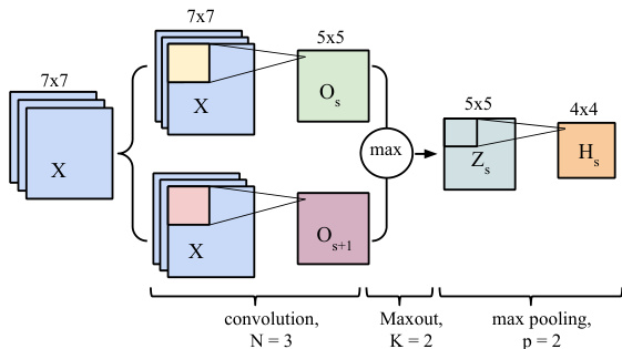
Figure 1: A single convolution layer block showing computations for a single feature map. The input patch (here $7\times7)$ , is convolved with series of kernels (here $3\times3$ ) followed by Maxout and max-pooling.
图 1: 展示单个特征图计算的卷积层模块。输入补丁 (此处为 $7\times7$ ) 与一系列卷积核 (此处为 $3\times3$ ) 进行卷积运算,后接Maxout和最大池化。
Whereas traditional image feature extraction methods rely on a fixed recipe (sometimes taking the form of convolution with a linear e.g. Gabor filter bank), the key to the success of convolutional neural networks is their ability to learn the weights and biases of individual feature maps, giving rise to data-driven, customized, task-specific dense feature extractors. These parameters are adapted via stochastic gradient descent on a surrogate loss function related to the mis classification error, with gradients computed efficiently via the back propagation algorithm [40].
传统图像特征提取方法依赖于固定模式(有时采用线性卷积形式,如Gabor滤波器组),而卷积神经网络成功的关键在于其能够学习各特征图的权重和偏置,从而形成数据驱动、定制化、任务专用的密集特征提取器。这些参数通过代理损失函数(与分类错误相关)的随机梯度下降进行调整,并借助反向传播算法[40]高效计算梯度。
Special attention must be paid to the treatment of border pixels by the convolution operation. Throughout our architecture, we employ the so-called valid-mode convolution, meaning that the filter response is not computed for pixel positions that are less than $\lfloor N/2\rfloor$ pixels away from the image border. An $N{\times}N$ filter convolved with an $M\times M$ input patch will result in a $Q\times Q$ output, where $Q=M-N+1$ . In Figure 1, $M=7$ , $N=3$ and thus $Q=5$ . Note that the size (spatial width and height) of the kernels are hyperparameters that must be specified by the user.
必须特别注意卷积操作对边界像素的处理。在我们的架构中,全程采用所谓的有效模式卷积 (valid-mode convolution),这意味着不会计算距离图像边界小于 $\lfloor N/2\rfloor$ 像素位置的滤波器响应。一个 $N{\times}N$ 滤波器与 $M\times M$ 输入块进行卷积后,将产生 $Q\times Q$ 的输出,其中 $Q=M-N+1$。在图 1 中,$M=7$,$N=3$,因此 $Q=5$。请注意,卷积核的尺寸(空间宽度和高度)是必须由用户指定的超参数。
- Non-linear activation function: To obtain features that are non-linear transformations of the input, an element-wise non-linearity is applied to the result of the kernel convolution. There are multiple choices for this non-linearity, such as the sigmoid, hyperbolic tangent and rectified linear functions [24], [16].
- 非线性激活函数:为了获得输入的非线性变换特征,需要对核卷积的结果进行逐元素的非线性处理。这种非线性有多种选择,例如sigmoid函数、双曲正切函数和修正线性函数 [24], [16]。
Recently, Goodfellow et al. [18] proposed a Maxout nonlinearity, which has been shown to be particularly effective at modeling useful features. Maxout features are associated with multiple kernels ${\bf W}{s}$ . This implies each Maxout map ${\bf{Z}}{s}$ is associated with $K$ feature maps : ${\mathbf{O}{s},\mathbf{O}{s+1},...,\mathbf{O}_{s+K-1}}$ . Note that in Figure 1, the Maxout maps are associated with $K=2$ feature maps. Maxout features correspond to taking the max over the feature maps $\mathbf{o}$ , individually for each spatial position:
最近,Goodfellow等人[18]提出了一种Maxout非线性激活函数,该方法被证明在建模有效特征方面特别高效。Maxout特征与多个核${\bf W}{s}$相关联。这意味着每个Maxout映射${\bf{Z}}{s}$对应$K$个特征图:${\mathbf{O}{s},\mathbf{O}{s+1},...,\mathbf{O}_{s+K-1}}$。注意在图1中,Maxout映射对应$K=2$个特征图。Maxout特征的计算方式是对特征图$\mathbf{o}$的每个空间位置单独取最大值:
$$
Z_{s,i,j}=*{max}{O_{s,i,j},O_{s+1,i,j},...,O_{s+K-1,i,j}}
$$
where $i,j$ are spatial positions. Maxout features are thus equivalent to using a convex activation function, but whose shape is adaptive and depends on the values taken by the kernels.
其中 $i,j$ 为空间位置。Maxout特征因此等同于使用一个凸激活函数,但其形状是自适应的,并取决于核所取的值。
- Max pooling: This operation consists of taking the maximum feature (neuron) value over sub-windows within each feature map. This can be formalized as follows:
- 最大池化 (Max pooling): 该操作通过提取每个特征图子窗口中的最大特征(神经元)值来实现。其数学表达如下:
$$
H_{s,i,j}=\operatorname*{max}{p}Z_{s,i+p,j+p},
$$
$$
H_{s,i,j}=\operatorname*{max}{p}Z_{s,i+p,j+p},
$$
where $p$ determines the max pooling window size. The sub-windows can be overlapping or not (Figure 1 shows an overlapping configuration). The max-pooling operation shrinks the size of the feature map. This is controlled by the pooling size $p$ and the stride hyper-parameter, which corresponds to the horizontal and vertical increments at which pooling sub-windows are positioned. Let $S$ be the stride value and $Q\times Q$ be the shape of the feature map before max-pooling. The output of the max-pooling operation would be of size $D\times D$ , where $D=(Q-p)/S+1$ . In Figure 1, since $Q=5,p=2,S=1$ , the max-pooling operation results into a $D=4$ output feature map. The motivation for this operation is to introduce invariance to local translations. This sub sampling procedure has been found beneficial in other applications [27].
其中 $p$ 决定了最大池化窗口的大小。子窗口可以重叠也可以不重叠 (图 1 展示了一个重叠配置)。最大池化操作会缩小特征图的尺寸,这由池化尺寸 $p$ 和步长超参数控制,后者对应于池化子窗口在水平和垂直方向上的定位增量。设 $S$ 为步长值,$Q\times Q$ 为最大池化前特征图的形状,则最大池化操作的输出尺寸为 $D\times D$,其中 $D=(Q-p)/S+1$。在图 1 中,由于 $Q=5,p=2,S=1$,最大池化操作得到 $D=4$ 的输出特征图。该操作的动机是引入对局部平移的不变性。这种子采样过程在其他应用中被证明是有益的 [27]。
Convolutional networks have the ability to extract a hierarchy of increasingly complex features which makes them very appealing. This is done by treating the output feature maps of a convolutional layer as input channels to the subsequent convolutional layer.
卷积网络能够提取出层次逐渐复杂的特征,这一特性使其极具吸引力。具体实现方式是将卷积层的输出特征图作为后续卷积层的输入通道。
From the neural network perspective, feature maps correspond to a layer of hidden units or neurons. Specifically, each coordinate within a feature map corresponds to an individual neuron, for which the size of its receptive field corresponds to the kernel’s size. A kernel’s value also represents the weights of the connections between the layer’s neurons and the neurons in the previous layer. It is often found in practice that the learned kernels resemble edge detectors, each kernel being tuned to a different spatial frequency, scale and orientation, as is appropriate for the statistics of the training data.
从神经网络的角度来看,特征图对应着一层隐藏单元或神经元。具体而言,特征图中的每个坐标对应一个单独的神经元,其感受野大小与卷积核尺寸一致。卷积核的值也代表了该层神经元与前一层神经元之间连接的权重。实践中经常发现,学习到的卷积核类似于边缘检测器,每个卷积核会根据训练数据的统计特性调整到不同的空间频率、尺度和方向。
Finally, to perform a prediction of the segmentation labels, we connect the last convolutional hidden layer to a convolutional output layer followed by a non-linearity (i.e. no pooling is performed). It is necessary to note that, for segmentation purposes, a conventional CNN will not yield an efficient test time since the output layer is typically fully connected. By using a convolution at the end, for which we have an efficient implementation, the prediction at test time for a whole brain will be 45 times faster. The convolution uses as many kernels as there are different segmentation labels (in our case five). Each kernel thus acts as the ultimate detector of tissue from one of the segmentation labels. We use the softmax nonlinearity which normalizes the result of the kernel convolutions into a multi nominal distribution over the labels. Specifically, let a be the vector of values at a given spatial position, it computes softmax(a) $=\exp(\mathbf{a})/Z$ where $\begin{array}{r}{Z=\sum_{c}\exp(a_{c})}\end{array}$ is a normaliza- tion constant. More details will be d iscussed in Section 4.
最后,为了预测分割标签,我们将最后一个卷积隐藏层连接到一个卷积输出层,后接一个非线性变换(即不进行池化操作)。需要注意的是,对于分割任务而言,传统CNN由于输出层通常采用全连接结构,无法实现高效的测试速度。通过在末端使用卷积操作(我们已实现高效运算),整个大脑的测试阶段预测速度将提升45倍。该卷积层使用的卷积核数量与分割标签类别数相同(本实验中为五个)。每个卷积核因此充当对应分割标签组织的最终检测器。我们采用softmax非线性函数,将卷积核运算结果归一化为标签上的多项式分布。具体而言,设a为给定空间位置上的值向量,其计算过程为softmax(a) $=\exp(\mathbf{a})/Z$,其中归一化常数 $\begin{array}{r}{Z=\sum_{c}\exp(a_{c})}\end{array}$。更多细节将在第4节讨论。
Noting $\mathbf{Y}$ as the segmentation label field over the input patch $\mathbf{X}$ , we can thus interpret each spatial position of the convolutional output layer as providing a model for the likelihood distribution $p(Y_{i j}|\mathbf{X})$ , where $Y_{i j}$ is the label at position $i,j$ . We get the probability of all labels simply by taking the product of each conditional $\begin{array}{r}{p({\bf Y}|{\bf X})=\prod_{i j}p(Y_{i j}|{\bf X})}\end{array}$ . Our approach thus performs a multiclass labelin g by assigning to each pixel the label with the largest probability.
将输入图像块$\mathbf{X}$上的分割标签场记为$\mathbf{Y}$,因此我们可以将卷积输出层的每个空间位置解释为似然分布$p(Y_{i j}|\mathbf{X})$的模型,其中$Y_{i j}$是位置$i,j$处的标签。通过将每个条件概率相乘$\begin{array}{r}{p({\bf Y}|{\bf X})=\prod_{i j}p(Y_{i j}|{\bf X})}\end{array}$,我们得到所有标签的概率。因此,我们的方法通过为每个像素分配概率最大的标签来实现多类标注。
3.1. The Architectures
3.1. 架构
Our description of CNNs so far suggests a simple architecture corresponding to a single stack of several convolutional layers. This configuration is the most commonly implemented architecture in the computer vision literature. However, one could imagine other architectures that might be more appropriate for the task at hand.
目前我们对CNN的描述表明,其简单架构对应于由多个卷积层组成的单一堆叠。这种配置是计算机视觉领域文献中最常见的实现架构。然而,我们可以设想其他可能更适合当前任务的架构。
In this work, we explore a variety of architectures by using the concatenation of feature maps from different layers as another operation when composing CNNs. This operation allows us to construct architectures with multiple computational paths, which can each serve a different purpose. We now describe the two types of architectures that we explore in this work.
在本工作中,我们通过将不同层的特征图拼接作为构建CNN的另一种操作,探索了多种架构。这一操作使我们能够构建具有多条计算路径的架构,每条路径可实现不同功能。下面将介绍本文研究的两种架构类型。
3.1.1. Two-pathway architecture
3.1.1. 双通路架构
This architecture is made of two streams: a pathway with smaller $7\times7$ receptive fields and another with larger $13\times13$ receptive fields. We refer to these streams as the local pathway and the global pathway, respectively. The motivation for this architectural choice is that we would like the prediction of the label of a pixel to be influenced by two aspects: the visual details of the region around that pixel and its larger “context”, i.e. roughly where the patch is in the brain.
该架构由两条通路组成:一条是具有较小 $7\times7$ 感受野的通路,另一条是具有较大 $13\times13$ 感受野的通路。我们分别将这些通路称为局部通路和全局通路。这种架构设计的动机是希望像素标签的预测能受到两方面的影响:该像素周围区域的视觉细节及其更大的"上下文"(即该脑区大致位于大脑中的位置)。
The full architecture along with its details is illustrated in Figure 2. We refer to this architecture as the TwoPathCNN. To allow for the concatenation of the top hidden layers of both pathways, we use two layers for the local pathway, with $3\times3$ kernels for the second layer. While this implies that the effective receptive field of features in the top layer of each pathway is the same, the global pathway’s para me tri z ation more directly and flexibly models features in that same area. The concatenation of the feature maps of both pathways is then fed to the output layer.
完整架构及其细节如图 2 所示。我们将此架构称为 TwoPathCNN。为了实现两条路径顶部隐藏层的拼接,我们在局部路径中使用了两层,第二层采用 $3\times3$ 核。虽然这意味着每条路径顶层特征的有效感受野相同,但全局路径的参数化能更直接灵活地建模相同区域的特征。最后将两条路径的特征图拼接后输入输出层。
3.1.2. Cascaded architectures
3.1.2. 级联架构
One disadvantage of the CNNs described so far is that they predict each segmentation label separately from each other. This is unlike a large number of segmentation methods in the literature, which often propose a joint model of the segmentation labels, effectively modeling the direct dependencies between spatially close labels. One approach is to define a conditional random field (CRF) over the labels and perform meanfield message passing inference to produce a complete segmentation. In this case, the final label at a given position is effectively influenced by the models beliefs about what the label is in the vicinity of that position.
目前描述的CNN有一个缺点,即它们各自独立预测每个分割标签。这与文献中的大量分割方法不同,后者通常提出分割标签的联合模型,有效建模空间相邻标签间的直接依赖关系。一种方法是在标签上定义条件随机场 (CRF) ,并通过平均场消息传递推理生成完整分割。此时,特定位置的最终标签实际上会受到模型对该位置邻近区域标签预测的影响。
On the other hand, inference in such joint segmentation methods is typically more computationally expensive than a simple feed-forward pass through a CNN. This is an important aspect that one should take into account if automatic brain tumor segmentation is to be used in a day-to-day practice.
另一方面,这类联合分割方法的推理过程通常比简单的CNN前向传播计算成本更高。若要在日常实践中应用自动脑肿瘤分割技术,这一点是需要考虑的重要因素。
Here, we describe CNN architectures that both exploit the efficiency of CNNs, while also more directly model the dependencies between adjacent labels in the segmentation. The idea is simple: since we’d like the ultimate prediction to be influenced by the model’s beliefs about the value of nearby labels, we propose to feed the output probabilities of a first CNN as additional inputs to the layers of a second CNN. Again, we do this by relying on the concatenation of convolutional layers. In this case, we simply concatenate the output layer of the first CNN with any of the layers in the second CNN. Moreover, we use the same two-pathway structure for both CNNs. This effectively corresponds to a cascade of two CNNs, thus we refer to such models as cascaded architectures.
在此,我们描述了一种既能利用CNN(卷积神经网络)高效性,又能更直接建模分割任务中相邻标签间依赖关系的CNN架构。其核心思想很简单:由于我们希望最终预测能受到模型对邻近标签值判断的影响,因此提出将第一个CNN的输出概率作为额外输入馈送到第二个CNN的各层中。我们依然通过卷积层的级联来实现这一点——具体而言,只需将第一个CNN的输出层与第二个CNN的任意层进行拼接。两个CNN均采用相同的双通路结构,这实质上构成了两个CNN的级联,故我们将此类模型称为级联架构。
In this work, we investigated three cascaded architectures that concatenate the first CNN’s output at different levels of the second CNN:
在本工作中,我们研究了三种级联架构,它们将第一个CNN的输出在第二个CNN的不同层级进行连接:
• Input concatenation: In this architecture, we provide the first CNN’s output directly as input to the second CNN. They are thus simply treated as additional image channels of the input patch. The details are illustrated in Figure 3a. We refer to this model as Input Cascade CNN. • Local pathway concatenation: In this architecture, we move up one layer in the local pathway and perform concatenation to its first hidden layer, in the second CNN. The details are illustrated in Figure 3b. We refer to this model as Local Cascade CNN. Pre-output concatenation: In this last architecture, we move to the very end of the second CNN and perform concatenation right before its output layer. This architecture is interesting, as it is similar to the computations made by one pass of mean-field inference [46] in a CRF whose pairwise potential functions are the weights in the output kernels. From this view, the output of the first CNN is the first iteration of mean-field, while the output of the second CNN would be the second iteration. The difference with regular mean-field however is that our CNN allows the output at one position to be influenced by its previous value, and the convolutional kernels are not the same in the first and second CNN. The details are illustrated in Figure 3c. We refer to this model as MF Cascade CNN.
• 输入拼接 (Input concatenation):在该架构中,我们将第一个CNN的输出直接作为第二个CNN的输入。这些输出被简单地视为输入图像块的额外通道。具体细节如图3a所示。我们将该模型称为输入级联CNN (Input Cascade CNN)。
• 局部路径拼接 (Local pathway concatenation):在该架构中,我们将拼接位置上移至局部路径的第一隐藏层,在第二个CNN中进行操作。具体细节如图3b所示。我们将该模型称为局部级联CNN (Local Cascade CNN)。
• 预输出拼接 (Pre-output concatenation):在最后一种架构中,我们将拼接位置移至第二个CNN的末端,在其输出层之前进行操作。该架构的特别之处在于,其计算方式类似于CRF中均值场推断 (mean-field inference) [46] 的单次迭代过程,其中成对势函数即为输出卷积核的权重。从这个角度看,第一个CNN的输出相当于均值场的第一轮迭代,而第二个CNN的输出则是第二轮迭代。但与常规均值场不同的是,我们的CNN允许某位置的输出受其前值影响,且两个CNN的卷积核并不相同。具体细节如图3c所示。我们将该模型称为MF级联CNN (MF Cascade CNN)。
3.2. Training
3.2. 训练
Gradient Descent. By interpreting the output of the convolutional network as a model for the distribution over segmentation labels, a natural training criteria is to maximize the probability of all labels in our training set or, equivalently, to minimize the negative log-probability $\begin{array}{r}{-\log p(\mathbf{Y}|\mathbf{X})=\sum_{i j}-\log p(Y_{i j}|\mathbf{X})}\end{array}$ for each labeled brain.
梯度下降。通过将卷积网络的输出解释为分割标签分布的概率模型,一个自然的训练标准是最大化训练集中所有标签的概率,或者等价地,最小化每个标注大脑的负对数概率 $\begin{array}{r}{-\log p(\mathbf{Y}|\mathbf{X})=\sum_{i j}-\log p(Y_{i j}|\mathbf{X})}\end{array}$。
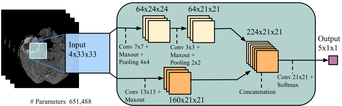
Figure 2: Two-pathway CNN architecture (TwoPathCNN). The figure shows the input patch going through two paths of convolutional operations. The feature-maps in the local and global paths are shown in yellow and orange respectively. The convolutional layers used to produce these feature-maps are indicated by dashed lines in the figure. The green box embodies the whole model which in later architectures will be used to indicate the TwoPathCNN.
图 2: 双通路CNN架构 (TwoPathCNN)。该图展示了输入图像块经过两条卷积运算路径的处理过程。局部路径和全局路径中的特征图分别用黄色和橙色表示。图中虚线标明了用于生成这些特征图的卷积层。绿色方框代表整个模型,在后续架构中将用于指代TwoPathCNN。
To do this, we follow a stochastic gradient descent approach by repeatedly selecting labels $Y_{i j}$ at a random subset of patches within each brain, computing the average negative log-probabilities for this mini-batch of patches and performing a gradient descent step on the CNNs parameters (i.e. the kernels at all layers).
为此,我们采用随机梯度下降方法:反复在每个大脑的随机子集选取标签 $Y_{ij}$,计算该小批量图像块的平均负对数概率,并对CNN参数(即所有层的卷积核)执行梯度下降步骤。
Performing updates based only on a small subset of patches allows us to avoid having to process a whole brain for each update, while providing reliable enough updates for learning. In practice, we implement this approach by creating a dataset of mini-batches of smaller brain image patches, paired with the corresponding center segmentation label as the target.
仅基于一小部分图像块(patch)进行更新,使我们能够避免每次更新都需要处理整个大脑,同时为学习提供足够可靠的更新。在实际操作中,我们通过创建小批量脑部图像块数据集来实现这一方法,并将对应的中心分割标签作为目标与之配对。
To further improve optimization, we implemented a so-called momentum strategy which has been shown successful in the past [27]. The idea of momentum is to use a temporally averaged gradient in order to damp the optimization velocity:
为了进一步优化,我们实现了一种所谓的动量策略 (momentum strategy),该策略在过去已被证明是成功的 [27]。动量策略的核心思想是利用时间平均梯度来抑制优化速度:
$$
\begin{array}{r c l}{\mathbf{V}{i+1}}&{=}&{\mu*\mathbf{V}{i}-\alpha*\nabla\mathbf{W}{i}}\ {\mathbf{W}{i+1}}&{=}&{\mathbf{W}{i}+\mathbf{V}_{i+1}}\end{array}
$$
$$
\begin{array}{r c l}{\mathbf{V}{i+1}}&{=}&{\mu*\mathbf{V}{i}-\alpha*\nabla\mathbf{W}{i}}\ {\mathbf{W}{i+1}}&{=}&{\mathbf{W}{i}+\mathbf{V}_{i+1}}\end{array}
$$
where $\mathbf{W}{i}$ stands for the CNNs parameters at iteration $i.$ , $\nabla\mathbf{W}{i}$ the gradient of the loss function at $\mathbf{W}_{i}$ , V is the integrated velocity initialized at zero, $\alpha$ is the learning rate, and $\mu$ the momentum coefficient. We define a schedule for the momentum $\mu$ where the momentum coefficient is gradually increased during training. In our experiments the initial momentum coefficient was set to $\mu=0.5$ and the final value was set to $\mu=0.9$ .
其中 $\mathbf{W}{i}$ 表示第 $i$ 次迭代时 CNN 的参数,$\nabla\mathbf{W}{i}$ 为 $\mathbf{W}_{i}$ 处的损失函数梯度,V 是初始化为零的累积速度,$\alpha$ 为学习率,$\mu$ 为动量系数。我们为动量 $\mu$ 设置了调度策略,在训练过程中逐步增大动量系数。实验中初始动量系数设为 $\mu=0.5$,最终值设为 $\mu=0.9$。
Also, the learning rate $\alpha$ is decreased by a factor at every epoch. The initial learning rate was set to $\alpha=0.005$ and the decay factor to $10^{-1}$ .
此外,学习率 $\alpha$ 在每个周期都会按一定比例衰减。初始学习率设为 $\alpha=0.005$,衰减因子为 $10^{-1}$。
Two-phase training. Brain tumor segmentation is a highly data imbalanced problem where the healthy voxels (i.e. label 0) comprise $98%$ of total voxels. From the remaining $2%$ pathological voxels, $0.18%$ belongs to necrosis (label 1), $1.1%$ to edema (label 2), $0.12%$ to non-enhanced (label 3) and $0.38%$ to enhanced tumor (label 4). Selecting patches from the true distribution would cause the model to be overwhelmed by healthy patches and causing problem when training out CNN models. Instead, we initially construct our patches dataset such that all labels are e qui probable. This is what we call the first training phase. Then, in a second phase, we account for the un-balanced nature of the data and re-train only the output layer (i.e. keeping the kernels of all other layers fixed) with a more representative distribution of the labels. This way we get the best of both worlds: most of the capacity (the lower layers) is used in a balanced way to account for the diversity in all of the classes, while the output probabilities are calibrated correctly (thanks to the re-training of the output layer with the natural frequencies of classes in the data).
两阶段训练。脑肿瘤分割是一个数据高度不平衡的问题,健康体素(即标签0)占总体的98%。在剩余的2%病理体素中,0.18%属于坏死(标签1),1.1%属于水肿(标签2),0.12%属于非增强(标签3),0.38%属于增强肿瘤(标签4)。若直接从真实分布中选取图像块,会导致模型被健康样本主导,从而影响CNN模型的训练效果。为此,我们首先构建一个各标签出现概率均等的图像块数据集,这被称为第一阶段训练。随后在第二阶段,我们考虑数据的不平衡特性,仅重新训练输出层(即固定其他所有层的卷积核参数),采用更接近真实情况的标签分布进行训练。这种方法兼顾了两方面优势:深层网络通过平衡训练充分学习各类别的多样性特征,而输出概率则通过基于真实类别频率的再训练得到准确校准。
Regular iz ation. Successful CNNs tend to be models with a lot of capacity, making them vulnerable to over fitting in a setting like ours where there clearly are not enough training examples. Accordingly, we found that regular iz ation is important in obtaining good results. Here, regular iz ation took several forms. First, in all layers, we bounded the absolute value of the kernel weights and applied both L1 and L2 regular iz ation to prevent over fitting. This is done by adding the regular iz ation terms to the negative log-probability (i.e. $-\log p(\mathbf{Y}|\mathbf{X})+\lambda_{1}|\mathbf{W}|{1}+$ $\lambda_{2}||\mathbf{W}||^{2}$ , where $\lambda_{1}$ and $\lambda_{2}$ are coefficients for L1 and L2 regularization terms respectively). L1 and L2 affect the parameters of the model in different ways, while L1 encourages sparsity, L2 encourages small values. We also used a validation set for early stopping, i.e. stop training when the validation performance stopped improving. The validation set was also used to tune the other hyper-parameters of the model. The reader shall note that the hyper-parameters of the model which includes using or not L2 and/or L1 coefficients were selected by doing a grid search over range of parameters. The chosen hyper-parameters were the ones for which the model performed best on a validation set.
正则化。成功的CNN往往具有很高的容量,这使得它们在我们这样明显缺乏足够训练样本的场景中容易过拟合。因此,我们发现正则化对获得良好结果至关重要。这里的正则化采取了多种形式:首先,在所有层中限制核权重的绝对值,并同时应用L1和L2正则化来防止过拟合。具体实现方式是将正则化项加入负对数概率(即$-\log p(\mathbf{Y}|\mathbf{X})+\lambda_{1}|\mathbf{W}|{1}+$$\lambda_{2}||\mathbf{W}||^{2}$,其中$\lambda_{1}$和$\lambda_{2}$分别为L1和L2正则化项的系数)。L1和L2以不同方式影响模型参数——L1促进稀疏性,L2促使参数值趋小。我们还采用验证集进行早停(即当验证性能停止提升时终止训练),该验证集也用于调整模型其他超参数。需要说明的是,包括是否使用L2/L1系数在内的所有超参数,都是通过网格搜索从参数范围内选取的,最终选择的超参数组合能使模型在验证集上达到最佳性能。
Moreover, we used Dropout [42], a recent regular iz ation method that works by stochastic ally adding noise in the computation of the hidden layers of the CNN. This is done by multiplying each hidden or input unit by 0 (i.e. masking) with a certain probability (e.g. 0.5), independently for each unit and training update. This encourages the neural network to learn (c) Cascaded architecture, using pre-output concatenation, which is an architecture with properties similar to that of learning using a limited number of mean-field inference iterations in a CRF (MF Cascade CNN).
此外,我们采用了Dropout [42]这一近期提出的正则化方法,其原理是在CNN隐藏层计算过程中随机引入噪声。具体实现时,会以特定概率(如0.5)将每个隐藏单元或输入单元独立置零(即掩码处理),并在每次训练更新时重新采样。这种方法能促使神经网络学习 (c)级联架构(采用预输出拼接结构),该架构具有类似于在CRF中使用有限次平均场推断迭代学习时的特性(MF级联CNN)。
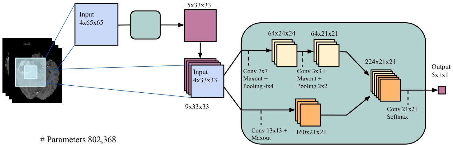
(a) Cascaded architecture, using input concatenation (Input Cascade CNN).
(a) 级联架构,使用输入串联 (Input Cascade CNN)。
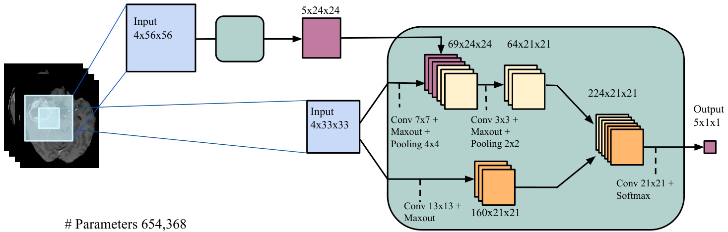
(b) Cascaded architecture, using local pathway concatenation (Local Cascade CNN).
(b) 级联架构,采用局部路径连接 (Local Cascade CNN)。
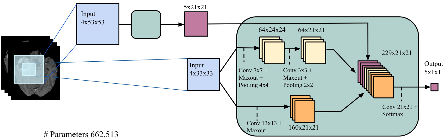
Figure 3: Cascaded architectures.
图 3: 级联架构。
features that are useful “on their own”, since each unit cannot assume that other units in the same layer won’t be masked as well and co-adapt its behavior. At test time, units are instead multiplied by one minus the probability of being masked. For more details, see Srivastava et al. [42].
具有独立实用性的特征,因为每个单元无法假设同层的其他单元不会被屏蔽并调整其行为。在测试时,单元会乘以未被屏蔽的概率。更多细节请参阅 Srivastava 等人 [42]。
Considering the large number of parameters our model has, one might think that even with our regular iz ation strategy, the 30 training brains from BRATS 2013 are too few to prevent over fitting. But as will be shown in the results section, our model generalizes well and thus do not overfit. One reason for this is the fact that each brain comes with 200 2d slices and thus, our model has approximately 6000 2D images to train on. We shall also mention that by their very nature, MRI images of brains are very similar from one patient to another. Since the variety of those images is much lower than those in realimage datasets such as CIFAR and ImageNet, a fewer number of training samples is thus needed.
考虑到我们的模型参数数量庞大,有人可能会认为即使采用常规的正则化策略,仅使用BRATS 2013提供的30个训练脑部数据仍不足以避免过拟合。但如结果部分所示,我们的模型展现出良好的泛化能力,因此并未出现过拟合现象。其中一个原因在于,每个脑部样本包含200张2D切片,这意味着模型实际上拥有约6000张2D图像进行训练。此外需要指出的是,脑部MRI图像本身具有高度相似性,不同患者间的差异远小于CIFAR和ImageNet等真实图像数据集。正因这类图像的多样性较低,所需的训练样本量也相应减少。
Cascaded Architectures. To train a cascaded architecture, we start by training the TwoPathCNN with the two phase stochastic gradient descent procedure described previously. Then, we fix the parameters of the TwoPathCNN and include it in the cascaded architecture (be it the Input Cascade CNN, the LocalCascadeCNN, or the MF Cascade CNN) and move to training the remaining parameters using a similar procedure. It should be noticed however that for the spatial size of the first CNN’s output and the layer of the second CNN to match, we must feed to the first CNN a much larger input. Thus, training of the second CNN must be performed on larger patches. For example in the Input Cascade CNN (Figure 3a), the input size to the first model is of size $65\times65$ which results into an output of size $33\times33$ . Only in this case the outputs of the first CNN can be concatenated with the input channels of the second CNN.
级联架构。为了训练级联架构,我们首先使用之前描述的两阶段随机梯度下降过程训练TwoPathCNN。然后,固定TwoPathCNN的参数并将其包含在级联架构中(无论是Input Cascade CNN、LocalCascadeCNN还是MF Cascade CNN),并继续使用类似过程训练剩余参数。但需注意的是,为了使第一个CNN的输出空间尺寸与第二个CNN的层相匹配,我们必须向第一个CNN输入更大的数据。因此,第二个CNN的训练必须在更大的图像块上进行。例如在Input Cascade CNN (图 3a) 中,第一个模型的输入尺寸为 $65\times65$,输出尺寸为 $33\times33$。只有在这种情况下,第一个CNN的输出才能与第二个CNN的输入通道进行拼接。
4. Implementation details
4. 实现细节
Our implementation is based on the Pylearn2 library [17]. Pylearn2 is an open-source machine learning library specializing in deep learning algorithms. It also supports the use of GPUs, which can greatly accelerate the execution of deep learning algorithms.
我们的实现基于Pylearn2库 [17]。Pylearn2是一个专注于深度学习算法的开源机器学习库,同时支持使用GPU来大幅加速深度学习算法的执行。
Since CNN’s are able to learn useful features from scratch, we applied only minimal pre-processing. We employed the same pre-processing as Tustison et al., the winner of the 2013 BRATS challenge [32]. The pre-processing follows three steps. First, the $1%$ highest and lowest intensities are removed. Then, we apply an N4ITK bias correction [3] to T1 and T1C modalities. The data is then normalized within each input channel by subtracting the channel’s mean and dividing by the channel’s standard deviation.
由于CNN能够从零开始学习有用的特征,我们仅应用了最少的预处理。我们采用了与2013年BRATS挑战赛冠军Tustison等人 [32] 相同的预处理方法。预处理分为三个步骤:首先,移除$1%$的最高和最低强度值;接着,对T1和T1C模态应用N4ITK偏置校正 [3];最后,通过减去通道均值并除以通道标准差,对每个输入通道内的数据进行归一化处理。
As for post-processing, a simple method based on connected components was implemented to remove flat blobs which might appear in the predictions due to bright corners of the brains close to the skull.
至于后处理,我们实现了一种基于连通分量的简单方法,用于移除预测中可能出现的扁平斑块,这些斑块源于靠近颅骨的脑部明亮角落。
The hyper-parameters of the different architectures (kernel and max pooling size for each layer and the number of layers) can be seen in Figure 3. Hyper-parameters were tuned using grid search and cross-validation on a validation set (see Bengio [6]). The chosen hyper-parameters were the ones for which the model performed best on the validation set. For max pooling, we always use a stride of 1. This is to keep per-pixel accuracy during full image prediction. We observed in practice that max pooling in the global path does not improve accuracy. We also found that adding additional layers to the architectures or increasing the capacity of the model by adding additional feature maps to the convolutional blocks do not provide any meaningful performance improvement.
不同架构的超参数(每层的卷积核大小和最大池化尺寸以及层数)可在图3中查看。超参数通过网格搜索和验证集交叉验证进行调优(参见Bengio [6])。所选超参数是模型在验证集上表现最佳的组合。对于最大池化,我们始终使用步长为1的设置,这是为了在全图预测时保持逐像素精度。实际观察发现,全局路径中的最大池化操作不会提升准确率。我们还发现,增加网络层数或通过为卷积块添加更多特征图来扩展模型容量,均未带来显著的性能提升。
Biases are initialized to zero except for the softmax layer for which we initialized them to the log of the label frequencies. The kernels are randomly initialized from $U\left(-0.005,0.005\right)$ . Training takes about 3 minutes per epoch for the TwoPathCNN model on an NVIDIA Titan black card.
除softmax层的偏置初始化为标签频率的对数外,其余偏置均初始化为零。卷积核从$U\left(-0.005,0.005\right)$中随机初始化。在NVIDIA Titan black显卡上,TwoPathCNN模型每个epoch的训练时间约为3分钟。
At test time, we run our code on a GPU in order to exploit its computational speed. Moreover, the convolutional nature of the output layer allows us to further accelerate computations at test time. This is done by feeding as input a full image and not individual patches. Therefore, convolutions at all layers can be extended to obtain all label probabilities $p(Y_{i j}|\mathbf{X})$ for the entire image. With this implementation, we are able to produce a segmentation in 25 seconds per brain on the Titan black card with the TwoPathCNN model. This turns out to be 45 times faster than when we extracted a patch at each pixel and processed them individually for the entire brain.
测试时,我们在GPU上运行代码以利用其计算速度。此外,输出层的卷积特性使我们能够进一步加速测试时的计算。具体做法是将整张图像而非单个图像块作为输入。因此,可以扩展所有层的卷积操作,从而一次性获取整张图像的所有标签概率 $p(Y_{i j}|\mathbf{X})$ 。通过这种实现方式,我们使用TwoPathCNN模型在Titan black显卡上对每个大脑进行分割仅需25秒,这比逐像素提取图像块并单独处理全脑数据的速度快45倍。
Predictions for the MF Cascade CNN model, the LocalCascadeCNN model, and Input Cascade CNN model take on average 1.5 minutes, 1.7 minutes and 3 minutes respectively.
MF Cascade CNN模型、LocalCascadeCNN模型和Input Cascade CNN模型的预测平均耗时分别为1.5分钟、1.7分钟和3分钟。
5. Experiments and Results
5. 实验与结果
The experiments were carried out on real patient data obtained from the 2013 brain tumor segmentation challenge (BRATS2013), as part of the MICCAI conference [15]. The BRATS2013 dataset is comprised of 3 sub-datasets. The training dataset, which contains 30 patient subjects all with pixelaccurate ground truth (20 high grade and 10 low grade tumors); the test dataset which contains 10 (all high grade tumors) and the leader board dataset which contains 25 patient subjects (21 high grade and 4 low grade tumors). There is no ground truth provided for the test and leader board datasets. All brains in the dataset have the same orientation. For each brain there exists 4 modalities, namely T1, T1C, T2 and Flair which are coregistered. The training brains come with ground truth for which 5 segmentation labels are provided, namely non-tumor, necrosis, edema, non-enhancing tumor and enhancing tumor. Figure 4 shows an example of the data as well as the ground truth. In total, the model iterates over about 2.2 million examples of tumorous patches (this consists of all the 4 sub-tumor classes) and goes through 3.2 million of the healthy patches. As mentioned before during the first phase training, the distribution of examples introduced to the model from all 5 classes is uniform.
实验采用2013年脑肿瘤分割挑战赛(BRATS2013)的真实患者数据开展,该数据集属于MICCAI会议组成部分[15]。BRATS2013数据集包含3个子集:训练集(30例患者,均具有像素级标注真值,含20例高级别和10例低级别肿瘤);测试集(10例,均为高级别肿瘤);排行榜数据集(25例患者,含21例高级别和4例低级别肿瘤)。测试集与排行榜数据集未提供标注真值。所有脑部数据具有相同空间方位,每例包含T1、T1C、T2和Flair四种已配准的模态影像。训练集提供5类分割标签的标注真值:非肿瘤、坏死、水肿、非强化肿瘤和强化肿瘤。图4展示了数据样例及对应标注。模型总计迭代约220万个肿瘤图像块样本(包含全部4类亚肿瘤组织)和320万个正常组织样本。如前述,第一阶段训练时模型接触的5类样本呈均匀分布。
Please note that we could not use the BRATS 2014 dataset due to problems with both the system performing the evaluation and the quality of the labeled data. For these reasons the old BRATS 2014 dataset has been removed from the official website and, at the time of submitting this manuscript, the BRATS website still showed: “Final data for BRATS 2014 to be released soon”. Furthermore, we have even conducted an experiment where we trained our model with the old 2014 dataset and made predictions on the 2013 test dataset; however, the performance was worse than our results mentioned in this paper. For these reasons, we decided to focus on the BRATS 2013 data.
请注意,由于评估系统运行问题和标注数据质量问题,我们无法使用BRATS 2014数据集。因此,旧的BRATS 2014数据集已从官网移除,截至本文投稿时,BRATS官网仍显示:"BRATS 2014最终数据即将发布"。此外,我们甚至进行了一项实验:用旧版2014数据集训练模型并在2013测试集上预测,但其表现逊于本文所述结果。基于这些原因,我们决定专注于BRATS 2013数据。

Figure 4: The first four images from left to right show the MRI modalities used as input channels to various CNN models and the fifth image shows the ground truth labels where $\cdot$ edema, $\cdot$ enhanced tumor, ■ necrosis, $\boldsymbol{\cdot}$ non-enhanced tumor.
图 4: 从左至右前四幅图像展示了作为各种CNN模型输入通道的MRI模态,第五幅图像显示了真实标签,其中$\cdot$表示水肿,$\cdot$表示增强肿瘤,■表示坏死,$\boldsymbol{\cdot}$表示非增强肿瘤。
As mentioned in Section 3, we work with 2D slices due to the fact that the MRI volumes in the dataset do not posses an isotropic resolution and the spacing in the third dimension is not consistent across the data. We explored the use of 3D information (by treating the third dimension as extra input channels or by having an architecture which takes orthogonal slices from each view and makes the prediction on the intersecting center pixel), but that didn’t improve performance and made our method very slow.
如第3节所述,我们采用2D切片进行处理,原因是数据集中MRI体数据不具备各向同性分辨率,且第三维间距在数据中不一致。我们尝试利用3D信息(将第三维度作为额外输入通道,或采用能接收各视图正交切片并对交叉中心像素进行预测的架构),但这并未提升性能,反而显著降低了方法速度。
Note that as suggested by Krizhevsky et al. [27], we applied data augmentation by flipping the input images. Unlike what was reported by Zeiler and Fergus [47], it did not improve the overall accuracy of our model.
需要注意的是,正如 Krizhevsky 等人 [27] 所建议的,我们通过翻转输入图像进行了数据增强。但与 Zeiler 和 Fergus [47] 报告的结果不同,这并没有提高我们模型的整体准确率。
Quantitative evaluation of the models performance on the test set is achieved by uploading the segmentation results to the online BRATS evaluation system [14]. The online system provides the quantitative results as follows: The tumor structures are grouped in 3 different tumor regions. This is mainly due to practical clinical applications. As described by Menze et al. [32], tumor regions are defined as:
通过将分割结果上传至在线BRATS评估系统[14],对模型在测试集上的性能进行定量评估。该系统提供的量化结果如下:肿瘤结构被划分为3个不同的肿瘤区域,这主要基于实际临床应用需求。如Menze等人[32]所述,肿瘤区域定义为:
a) The complete tumor region (including all four tumor structures). b) The core tumor region (including all tumor structures exept “edema”). c) The enhancing tumor region (including the “enhanced tumor” structure).
a) 完整肿瘤区域 (包含所有四种肿瘤结构)。
b) 核心肿瘤区域 (包含除"水肿"外的所有肿瘤结构)。
c) 增强肿瘤区域 (包含"增强肿瘤"结构)。
For each tumor region, Dice (identical to F measure), Sensitivity and Specificity are computed as follows :
对于每个肿瘤区域,Dice (等同于F值)、敏感性和特异性按如下方式计算:
$$
\begin{array}{r c l}{{D i c e(P,T)}}&{{=}}&{{\displaystyle\frac{|P_{1}\wedge T_{1}|}{(|P_{1}|+|T_{1}|)/2},}}\ {{}}&{{}}&{{}}\ {{S e n s i t i\nu i t y(P,T)}}&{{=}}&{{\displaystyle\frac{|P_{1}\wedge T_{1}|}{|T_{1}|},}}\ {{}}&{{}}&{{}}\ {{S p e c i f i c i t y(P,T)}}&{{=}}&{{\displaystyle\frac{|P_{0}\wedge T_{0}|}{|T_{0}|},}}\end{array}
$$
$$
\begin{array}{r c l}{{D i c e(P,T)}}&{{=}}&{{\displaystyle\frac{|P_{1}\wedge T_{1}|}{(|P_{1}|+|T_{1}|)/2},}}\ {{}}&{{}}&{{}}\ {{S e n s i t i\nu i t y(P,T)}}&{{=}}&{{\displaystyle\frac{|P_{1}\wedge T_{1}|}{|T_{1}|},}}\ {{}}&{{}}&{{}}\ {{S p e c i f i c i t y(P,T)}}&{{=}}&{{\displaystyle\frac{|P_{0}\wedge T_{0}|}{|T_{0}|},}}\end{array}
$$
where $P$ represents the model predictions and $T$ represents the ground truth labels. We also note as $T_{1}$ and $T_{0}$ the subset of voxels predicted as positives and negatives for the tumor region in question. Similarly for $P_{1}$ and $P_{0}$ . The online evaluation system also provides a ranking for every method submitted for evaluation. This includes methods from the 2013 BRATS challenge published in [32] as well as anonymized unpublished methods for which no reference is available. In this section, we report experimental results for our different CNN architectures.
其中 $P$ 代表模型预测值,$T$ 代表真实标签。我们将肿瘤区域预测为阳性和阴性的体素子集分别记为 $T_{1}$ 和 $T_{0}$,同理定义 $P_{1}$ 和 $P_{0}$。在线评估系统还会为每种提交评估的方法提供排名,这些方法包括2013年BRATS挑战赛中发表的方法 [32] ,以及无法获取参考文献的匿名未发表方法。本节将汇报我们不同CNN架构的实验结果。
5.1. The TwoPathCNN architecture
5.1. TwoPathCNN 架构
As mentioned previously, unlike conventional CNNs, the TwoPathCNN architecture has two pathways: a “local” path focusing on details and a “global” path more focused on the context. To better understand how joint training of the global and local pathways benefits the performance, we report results on each pathway as well as results on averaging the outputs of each pathway when trained separately. Our method also deals with the unbalanced nature of the problem by training in two phases as discussed in Section 3.2. To see the impact of the two phase training, we report results with and without it. We refer to the CNN model consisting of only the local path (i.e. conventional CNN architecture) as Local Path CNN, the CNN model consisting of only the global path as Global Path CNN, the model averaging the outputs of the local and global paths (i.e. Local Path CNN and Global Path CNN) as AverageCNN and the two-pathway CNN architecture as TwoPathCNN. The second training phase is noted by appending ‘*’ to the architecture name. Since the second phase training has a substantial effect and always improves the performance, we only report results on Global Path CNN and AverageCNN with the second phase.
如前所述,与传统CNN不同,TwoPathCNN架构包含两条路径:专注于细节的"局部"路径和更关注上下文的"全局"路径。为了更好地理解全局与局部路径联合训练对性能的提升效果,我们分别报告了各路径单独训练时的结果,以及两条路径输出平均值的结果。如第3.2节所述,我们的方法还通过两阶段训练解决了数据不平衡问题。为评估两阶段训练的影响,我们对比了使用与不使用该策略的结果。
我们将仅包含局部路径(即传统CNN架构)的模型称为Local Path CNN,仅包含全局路径的模型称为Global Path CNN,对两条路径输出取平均的模型称为AverageCNN,完整双路径架构称为TwoPathCNN。第二阶段训练通过在架构名称后添加"*"标注。由于第二阶段训练能显著提升性能,我们仅报告带第二阶段训练的Global Path CNN和AverageCNN结果。
Table 1 presents the quantitative results of these variations. This table contains results for the TwoPathCNN with one and two training phases, the common single path CNN (i.e. LocalPathCNN) with one and two training phases, the Global $\mathrm{ParaCNN^{*}}$ which is a single path CNN model following the global pathway architecture and the output average of each of the trained single-pathway models (AverageCNN*). Without much surprise, the single path with one training phase CNN was ranked last with the lowest scores on almost every region. Using a second training phase gave a significant boost to that model with a rank that went from 15 to 9. Also, the table shows that joint training of the local and global paths yields better performance compared to when each pathway is trained separately and the outputs are averaged. One likely explanation is that by joint training the local and global paths, the model allows the two pathways to co-adapt. In fact, the AverageCNN* performs worse than the Local Path CNN* due to the fact that the GlobalPathCNN* performs very badly. The top performing method in the uncascaded models is the TwoPathCNN* with a rank of 4.
表 1: 呈现了这些变体的量化结果。该表格包含以下模型的性能数据:单阶段和双阶段训练的TwoPathCNN、单阶段和双阶段训练的普通单路径CNN (即LocalPathCNN)、采用全局路径架构的单路径CNN模型Global $\mathrm{ParaCNN^{}}$,以及各单路径训练模型输出平均值(AverageCNN)。不出所料,单阶段训练的单路径CNN在几乎所有区域都排名垫底。采用第二阶段训练后,该模型排名从15位显著提升至第9位。此外,表格显示局部路径与全局路径联合训练的性能优于单独训练各路径后取输出平均值的方法。一个可能的解释是:通过联合训练,模型使两条路径能够协同适应。事实上,由于GlobalPathCNN表现极差,AverageCNN的性能甚至低于LocalPathCNN*。在非级联模型中表现最佳的是排名第4的TwoPathCNN*。
Also, in some cases results are less accurate over the Enhancing region than for the Core and Complete regions. There are 2 main reasons for that. First, borders are usually diffused and there are no clear cut between enhanced tumor and nonenhanced tissues. This creates problems for both user labeling, ground truth, as well as the model. The second reason is that the model learns what it sees in the ground truth. Since the labels are created by different people and since the borders are not clear, each user has a slightly different interpretation of the borders of the enhanced tumor and so sometimes we see overly thick enhanced tumor in the ground truth.
此外,在某些情况下,增强区域(Enhancing region)的结果准确性低于核心区域(Core region)和完整区域(Complete region)。这主要有两个原因:首先,肿瘤增强区边界通常较为模糊,增强肿瘤与非增强组织之间缺乏明确分界。这种情况既给人工标注和基准真值(ground truth)带来困难,也影响了模型性能。其次,模型学习的是基准真值中的标注数据。由于标注由不同人员完成且边界不清晰,每个标注者对增强肿瘤边界的判定存在细微差异,因此我们有时会在基准真值中看到过厚的增强肿瘤轮廓。

Figure 5: Randomly selected filters from the first layer of the model. From left to right the figure shows visualization of features from the first layer of the global and local path respectively. Features in the local path include more edge detectors while the global path contains more localized features.
图 5: 从模型第一层随机选取的滤波器。从左至右分别展示了全局路径和局部路径第一层的特征可视化。局部路径中的特征包含更多边缘检测器,而全局路径则包含更多局部化特征。
Figure 5 shows representation of low level features in both local and global paths. As seen from this figure, features in the local path include more edge detectors while the ones in the global path are more localized features. Unfortunately, visualizing the learned mid/high level features of a CNN is still very much an open research problem. However, we can study the impact these features have on predictions by visualizing the segmentation results of different models. The segmentation results on two subjects from our validation set, produced by different variations of the basic model can be viewed in Figure $7^{5}$ . As shown in the figure, the two-phase training procedure allows the model to learn from a more realistic distribution of labels and thus removes false positives produced by the model which trains with one training phase. Moreover, by having two pathways, the model can simultaneously learn the global contextual features as well as the local detailed features. This gives the advantage of correcting labels at a global scale as well as recognizing fine details of the tumor at a local scale, yielding a better segmentation as oppose to a single path architecture which results in smoother boundaries. Joint training of the two convolutional pathways and having two training phases achieves better results.
图 5 展示了局部路径和全局路径中低级特征的表征。从图中可以看出,局部路径中的特征包含更多边缘检测器,而全局路径中的特征则更为局部化。遗憾的是,可视化卷积神经网络(CNN)学习到的中/高级特征仍然是一个开放的研究问题。不过,我们可以通过可视化不同模型的分割结果来研究这些特征对预测的影响。基础模型不同变体在验证集上对两个受试者产生的分割结果如图 $7^{5}$ 所示。如图所示,两阶段训练过程使模型能够从更真实的标签分布中学习,从而消除了单阶段训练模型产生的假阳性结果。此外,通过双路径设计,模型可以同时学习全局上下文特征和局部细节特征。这种架构优势在于既能从全局尺度修正标签,又能从局部尺度识别肿瘤的精细细节,相比单路径架构产生的平滑边界能获得更好的分割效果。两个卷积路径的联合训练配合两阶段训练策略取得了更优的结果。
5.2. Cascaded architectures
5.2. 级联架构
We now discuss our experiments with the three cascaded architectures namely Input Cascade CNN, Local Cascade CNN and MF Cascade CNN. Table 2 provides the quantitative results for each architecture. Figure 7 also provides visual examples of the segmentation generated by each architecture.
我们现在讨论三种级联架构的实验,分别是输入级联CNN、局部级联CNN和MF级联CNN。表2提供了每种架构的定量结果。图7还展示了各架构生成的分割视觉示例。
We find that the MF Cascade CNN* model yields smoother boundaries between classes. We hypothesize that, since the neurons in the softmax output layer are directly connected to the previous outputs within each receptive field, these parameters are more likely to learn that the center pixel label should have a similar label to its surroundings.
我们发现MF Cascade CNN*模型在类别间产生了更平滑的边界。我们假设,由于softmax输出层中的神经元直接连接到每个感受野内的先前输出,这些参数更可能学习到中心像素标签应与其周围环境具有相似的标签。

Figure 8: Visual results from our top performing model, Input Cascade CNN* on Coronal and Sagittal views. The subjects are the same as in Figure 7. In every sub-figure, the top row represents the Sagital view and the bottom row represents the Coronal view. The color codes are as follows: ■ edema, enhanced tumor, $\cdot$ necrosis, $\boldsymbol{\cdot}$ non-enhanced tumor.
图 8: 我们表现最佳的模型 Input Cascade CNN* 在冠状面和矢状面上的可视化结果。受试者与图 7 相同。每个子图中,顶部为矢状面视图,底部为冠状面视图。颜色编码如下:■ 水肿 (edema)、■ 强化肿瘤 (enhanced tumor)、$\cdot$ 坏死 (necrosis)、$\boldsymbol{\cdot}$ 非强化肿瘤 (non-enhanced tumor)。
As for the Local Cascade CNN* architecture, while it resulted in fewer false positives in the complete tumor category, the performance in other categories (i.e. tumor core and enhanced tumor) did not improve.
至于 Local Cascade CNN* 架构,虽然在完整肿瘤类别中减少了误报,但在其他类别(即肿瘤核心和增强肿瘤)的性能并未提升。
Figure 8 shows segmentation results from the same brains (as in Figure 7) in Sagittal and Coronal views. The InputCascadeCNN* model was used to produce these results. As seen from this figure, although the segmentation is performed on Axial view but the output is consistent in Coronal and Sagittal views. Although subjects in Figure 5 and Figure 6 are from our validation set for which the model is not trained on and the segmentation results from these subjects can give a good estimate of the models performance on a test set, however, for further clarity we visualise the models performance on two subjects from BRATS-2013 testst. These results are shown in Figure 9 in Saggital (top) and Axial (bottom) views.
图 8 展示了同一组大脑(与图 7 相同)在矢状面和冠状面的分割结果。这些结果由 InputCascadeCNN* 模型生成。如图所示,虽然分割是在轴状面进行的,但输出结果在冠状面和矢状面保持一致。尽管图 5 和图 6 中的受试者来自我们的验证集(模型未针对该数据集进行训练),这些受试者的分割结果可以很好地评估模型在测试集上的性能,但为了更清晰地展示,我们可视化了模型在 BRATS-2013 测试集中两名受试者上的表现。这些结果如图 9 所示,分别为矢状面(上)和轴状面(下)视图。
To better understand the process for which InputCascadeCNN* learns features, we present in Figure 6 the progression of the model by making predictions at every few epochs on a subject from our validation set.
为了更好地理解InputCascadeCNN*学习特征的过程,我们在图6中展示了模型通过在验证集上每隔几个周期进行预测的进展情况。
Overall, the best performance is reached by the InputCascadeCNN* model. It improves the Dice measure on all tumor regions. With this architecture, we were able to reach the second rank on the BRATS 2013 scoreboard. While MFCascadeCNN*, TwoPathCNN* and Local Cascade CNN* are all ranked 4, the inner ranking between these three models is noted as 4a, 4b and $_{4\mathtt{C}}$ respectively.
总体而言,InputCascadeCNN* 模型取得了最佳性能。该模型在所有肿瘤区域的 Dice 指标上均有所提升。凭借这一架构,我们在 BRATS 2013 排行榜上获得了第二名。虽然 MFCascadeCNN*、TwoPathCNN* 和 Local Cascade CNN* 均排名第4,但这三个模型之间的内部排名分别标注为 4a、4b 和 $_{4\mathtt{C}}$。

Figure 6: Progression of learning in Input Cascade CNN*. The stream of figures on the first row from left to right show the learning process during the first phase. As the model learns better features, it can better distinguish boundaries between tumor sub-classes. This is made possible due to uniform label distribution of patches during the first phase training which makes the model believe all classes are e qui probable and causes some false positives. This drawback is alleviated by training a second phase (shown in second row from left to right) on a distribution closer to the true distribution of labels. The color codes are as follows: ■ edema, ■ enhanced tumor, ■ necrosis, $\cdot$ non-enhanced tumor.
图 6: Input Cascade CNN* 的学习进展。第一行从左到右的图像流展示了第一阶段的学习过程。随着模型学习到更好的特征,它能够更好地区分肿瘤亚类之间的边界。这是由于第一阶段训练中标签分布的均匀性,使模型认为所有类别出现的概率相同,从而导致一些假阳性。通过在更接近真实标签分布的分布上进行第二阶段训练(第二行从左到右展示),这一缺点得到了缓解。颜色编码如下:■ 水肿,■ 增强肿瘤,■ 坏死,$\cdot$ 非增强肿瘤。
Table 1: Performance of the TwoPathCNN model and variations. The second phase training is noted by appending ‘*’ to the architecture name. The ‘Rank’ column represents the ranking of each method in the online score board at the time of submission.
表 1: TwoPathCNN模型及其变体的性能表现。第二阶段训练通过在架构名称后添加"*"标注。"Rank"列表示提交时各方法在在线排行榜中的排名。
| Rank | Method | Complete | Core | Enhancing | Complete | Core | Enhancing | Complete | Core | Enhancing |
|---|---|---|---|---|---|---|---|---|---|---|
| 4 | TwoPATHCNN* | 0.85 | 0.78 | 0.73 | 0.93 | 0.80 | 0.72 | 0.80 | 0.76 | 0.75 |
| 9 | LOCALPATHCNN* | 0.85 | 0.74 | 0.71 | 0.91 | 0.75 | 0.71 | 0.80 | 0.77 | 0.73 |
| 10 | AVERAGECNN* | 0.84 | 0.75 | 0.70 | 0.95 | 0.83 | 0.73 | 0.77 | 0.74 | 0.73 |
| 14 | GLOBALPATHCNN* | 0.82 | 0.73 | 0.68 | 0.93 | 0.81 | 0.70 | 0.75 | 0.65 | 0.70 |
| 14 | TwOPATHCNN | 0.78 | 0.63 | 0.68 | 0.67 | 0.50 | 0.59 | 0.96 | 0.89 | 0.82 |
| 15 | LOCALPATHCNN | 0.77 | 0.64 | 0.68 | 0.65 | 0.52 | 0.60 | 0.96 | 0.87 | 0.80 |

Figure 7: Visual results from our CNN architectures from the Axial view. For each sub-figure, the top row from left to right shows T1C modality, the conventional one path CNN, the Conventional CNN with two training phases, and the TwoPathCNN model. The second row from left to right shows the ground truth, Local Cascade CNN model, the MF Cascade CNN model and the Input Cascade CNN. The color codes are as follows: $\cdot$ edema, $\cdot$ enhanced tumor, $\cdot$ necrosis, $\cdot$ non-enhanced tumor.
图 7: 我们CNN架构在轴向视图中的可视化结果。每个子图中,第一行从左到右依次显示T1C模态、传统单路径CNN、采用两阶段训练的传统CNN以及TwoPathCNN模型。第二行从左到右展示真实标注、Local Cascade CNN模型、MF Cascade CNN模型和Input Cascade CNN模型。颜色标识如下:$\cdot$水肿、$\cdot$强化肿瘤、$\cdot$坏死、$\cdot$非强化肿瘤。
Table 2: Performance of the cascaded architectures. The reported results are from the second phase training. The ‘Rank’ column shows the ranking of each method in the online score board at the time of submission.
表 2: 级联架构的性能表现。报告结果来自第二阶段训练。"Rank"列显示了提交时每种方法在在线排行榜中的排名。
| Rank | Method | Complete | Core | Enhancing | Complete | Core | Enhancing | Complete | Core | Enhancing |
|---|---|---|---|---|---|---|---|---|---|---|
| 2 | INPUTCASCADECNN* | 0.88 | 0.79 | 0.73 | 0.89 | 0.79 | 0.68 | 0.87 | 0.79 | 0.80 |
| 4-a | MFCASCADECNN* | 0.86 | 0.77 | 0.73 | 0.92 | 0.80 | 0.71 | 0.81 | 0.76 | 0.76 |
| 4-c | LOCALCASCADECNN* | 0.88 | 0.76 | 0.72 | 0.91 | 0.76 | 0.70 | 0.84 | 0.80 | 0.75 |

Figure 9: Visual segmentation results from our top performing model, Input Cascade CNN*, on examples of the BRATS2013 test dataset in Saggital (top) and Axial (bottom) views. The color codes are as follows: ■ edema, ■ enhanced tumor, necrosis, $\boldsymbol{\cdot}$ non-enhanced tumor.
图 9: 我们表现最佳的模型 Input Cascade CNN* 在 BRATS2013 测试数据集上的视觉分割结果,展示了矢状面(上)和轴向面(下)视图。颜色编码如下: ■ 水肿, ■ 增强肿瘤, 坏死, $\boldsymbol{\cdot}$ 非增强肿瘤。
Table 3 shows how our implemented architectures compare with currently published state-of-the-art methods as mentioned in $[32]^{6}$ . The table shows that Input Cascade CNN* out performs Tustison et al. the winner of the BRATS 2013 challenge and is ranked first in the table. Results from the BRATS-2013 leader board presented in Table 4 shows that our method outperforms other approaches on this dataset. We also compare our top performing method in Table 5 with state-of-the-art methods on BRATS-2012, ”4 label” test set as mentioned in [32]. As seen from this table, our method out performs other methods in the tumor Core category and gets competitive results on other categories.
表 3 展示了我们实现的架构与 $[32]^{6}$ 中提到的当前已发表的最先进方法的对比情况。该表显示,Input Cascade CNN* 的表现优于 BRATS 2013 挑战赛冠军 Tustison 等人,并在表中排名第一。表 4 展示了 BRATS-2013 排行榜的结果,表明我们的方法在该数据集上优于其他方法。我们还在表 5 中将我们的最佳表现方法与 [32] 中提到的 BRATS-2012 "4标签"测试集上的最先进方法进行了比较。从该表可以看出,我们的方法在肿瘤核心 (tumor Core) 类别中优于其他方法,并在其他类别中取得了具有竞争力的结果。
Let us mention that Tustison’s method takes 100 minutes to compute predictions per brain as reported in [32], while the Input Cascade CNN* takes 3 minutes, thanks to the fully convolutional architecture and the GPU implementation, which is over 30 times faster than the winner of the challenge. The TwoPathCNN* has a performance close to the state-of-the-art. However, with a prediction time of 25 seconds, it is over 200 times faster than Tustison’s method. Other top methods in the table are that of Meier et al and Reza et al with processing times of 6 and 90 minutes respectively. Recently Subbanna et al. [43] published competitive results on the BRATS 2013 dataset, reporting dice measures of 0.86, 0.86, 0.77 for Complete, Core and Enhancing tumor regions. Since they do not report Specificity and Sensitivity measures, a completely fair comparison with that method is not possible. However, as mentioned in [43], their method takes 70 minutes to process a subject, which is about 23 times slower than our method.
需要指出的是,据[32]报道,Tustison的方法每例大脑预测耗时100分钟,而得益于全卷积架构和GPU实现,Input Cascade CNN仅需3分钟完成预测,比该挑战赛冠军方案快30倍以上。TwoPathCNN的性能接近最先进水平,但其25秒的预测速度比Tustison方法快200多倍。表中其他领先方法包括Meier等人和Reza等人的方案,处理时间分别为6分钟和90分钟。最近Subbanna等人在[43]中发布了BRATS 2013数据集上的竞争性结果,报告完整肿瘤区、核心区和增强区的dice值分别为0.86、0.86、0.77。由于未报告特异性(Specificity)和敏感性(Sensitivity)指标,无法与该方案进行完全公平的比较。但如[43]所述,他们的方法处理单个病例需70分钟,比我们的方案慢约23倍。
Regarding other methods using CNNs, Urban et al. [45] used an average of two 3D convolutional networks with dice measures of 0.87, 0.77, 0.73 for Complete, Core and Enhancing tumor regions on BRATS 2013 test dataset with a prediction time of about 1 minute per model which makes for a total of $2\mathrm{min}.$ - utes. Again, since they do not report Specificity and Sensitivity measures, we can not make a full comparison. However, based on their dice scores our TwoPathCNN* is similar in performance while taking only 25 seconds, which is four times faster. And the Input Cascade CNN* is better or equal in accuracy while having the same processing time. As for [49], they do not report results on BRATS 2013 test dataset. However, their method is very similar to the Local Path CNN which, according to our experiments, has worse performance.
关于其他使用CNN的方法,Urban等人[45]在BRATS 2013测试集上采用两个3D卷积网络的平均结果,其Complete、Core和Enhancing肿瘤区域的dice值分别为0.87、0.77、0.73,单个模型预测时间约1分钟,总耗时$2\mathrm{min}$。由于未报告特异性(Specificity)和敏感性(Sensitivity)指标,我们无法进行全面对比。但就dice分数而言,我们的TwoPathCNN*在仅耗时25秒(提速四倍)的情况下达到相近性能,而Input Cascade CNN*在相同处理时间内取得更优或相当的精度。文献[49]未报告BRATS 2013测试集结果,但该方法与Local Path CNN高度相似,而我们的实验表明后者性能较差。
Table 5: Comparison of our top implemented architectures with the state-of-the-art methods on the BRATS-2012 ”4 label” test set as discussed in [32].
表 5: 我们的顶级实现架构与[32]中讨论的BRATS-2012"4标签"测试集上最先进方法的对比。
| 方法 | Dice | ||
|---|---|---|---|
| Complete | Core | Enhancing | |
| INPUTCASCADECNN* | 0.81 | 0.72 | 0.58 |
| Subbanna | 0.75 | 0.70 | 0.59 |
| Zhao | 0.82 | 0.66 | 0.42 |
| Tustison | 0.75 | 0.55 | 0.52 |
| Festa | 0.62 | 0.50 | 0.61 |
Using our best performing method, we took part in the BRATS 2015 challenge. The BRATS 2015 training dataset comprises of 220 subjects with high grade and 54 subjects with low grade gliomas. There are 53 subjects with mixed high and low grade gliomas for testing. Every participating group had 48 hours from receiving the test subjects to process them and submit their segmentation results to the online evaluation system. BRATS’15 contains the training data of 2013. The ground truth for the rest of the training brains is generated by a voted average of segmented results of the top performing methods in BRATS’13 and BRATS’12. Some of these automatically generated ground truths have been refined manually by a user.
采用我们表现最佳的方法,我们参与了BRATS 2015挑战赛。BRATS 2015训练数据集包含220例高级别胶质瘤患者和54例低级别胶质瘤患者,另有53例混合高低级别胶质瘤患者用于测试。各参赛团队在接收测试样本后有48小时进行处理,并将分割结果提交至在线评估系统。BRATS'15包含了2013年的训练数据,其余训练脑部数据的真实标签是通过对BRATS'13和BRATS'12中表现最佳方法的分割结果进行投票平均生成的,其中部分自动生成的真实标签已由用户手动修正。
Because distribution of the intensity values in this dataset is very variable from one subject to another, we used a 7 fold cross validation for training. At test time, a voted average of these models was made to make prediction for each subject in the test dataset. The results of the challenge are presented in Figure 10. The semi-automatic methods participating in the challenge have been highlighted in grey. Please note since these results are not yet publicly available, we refrain from disclosing the name of the participants. In this figure the semi-automatic methods are highlighted in gray. As seen from the figure, our method ranks either first or second on Complete tumor and tumor Core categories and gets competitive results on active tumor category. Our method has also less outliers than most other approaches.
由于该数据集中不同受试者的强度值分布差异较大,我们采用了7折交叉验证进行训练。测试时,对这些模型的投票平均值进行预测,以评估测试数据集中的每个受试者。挑战赛结果如图10所示,其中半自动方法以灰色高亮显示。请注意,由于这些结果尚未公开,我们暂不透露参与者名称。如图所示,我们的方法在完整肿瘤(Complete tumor)和肿瘤核心(tumor Core)类别中排名第一或第二,并在活跃肿瘤(active tumor)类别中取得具有竞争力的结果。与其他大多数方法相比,我们的方法异常值也更少。
6. Conclusion
6. 结论
In this paper, we presented an automatic brain tumor segmentation method based on deep convolutional neural networks. We considered different architectures and investigated their impact on the performance. Results from the BRATS 2013 online evaluation system confirms that with our best model we managed to improve on the currently published state-of-the-art method both on accuracy and speed as presented in MICCAI
本文提出了一种基于深度卷积神经网络(Deep Convolutional Neural Networks)的自动脑肿瘤分割方法。我们比较了不同网络架构并研究了其对性能的影响。BRATS 2013在线评估系统的结果表明,我们提出的最佳模型在准确性和速度上都超越了MICCAI会议上当前发表的最先进方法。

Figure 10: Our BRATS’15 challenge results using InputCascadeCNN*. Dice scores and negative log Hausdorff distances are presented for the three tumor categories. Since the results of the challenge are not yet publicly available, we are unable to disclose the name of the participants. The semi-automatic methods are highlighted in gray. In each sub-figure, the methods are ranked based on the mean value. The mean is presented in green, the median in red and outliers in blue.
图 10: 使用InputCascadeCNN*的BRATS'15挑战赛结果。针对三种肿瘤类别展示了Dice分数和负对数Hausdorff距离。由于挑战赛结果尚未公开,我们无法透露参与者姓名。半自动方法以灰色高亮显示。在每个子图中,方法根据平均值排序。绿色表示均值,红色表示中位数,蓝色表示离群值。
- The high performance is achieved with the help of a novel two-pathway architecture (which can model both the local details and global context) as well as modeling local label dependencies by stacking two CNN’s. Training is based on a two phase procedure, which we’ve found allows us to train CNNs efficiently when the distribution of labels is unbalanced.
2013年。高性能的实现得益于一种新颖的双路径架构(能够同时建模局部细节和全局上下文)以及通过堆叠两个CNN来建模局部标签依赖关系。训练采用两阶段流程,我们发现这种方法能在标签分布不均衡时高效训练CNN。
Thanks to the convolutional nature of the models and by using an efficient GPU implementation, the resulting segmentation system is very fast. The time needed to segment an entire brain with any of the these CNN architectures varies between 25 seconds and 3 minutes, making them practical segmentation methods.
得益于模型的卷积特性以及高效的GPU实现,所构建的分割系统运行速度极快。采用这些CNN架构对整个大脑进行分割所需时间介于25秒至3分钟之间,使其成为实用的分割方法。
References
参考文献
References
参考文献
Table 3: Comparison of our implemented architectures with the state-of-the-art methods on the BRATS-2013 test set.
表 3: 我们的实现架构与BRATS-2013测试集上最先进方法的对比
| 方法 | Dice (Complete) | Dice (Core) | Dice (Enhancing) | Specificity (Complete) | Specificity (Core) | Specificity (Enhancing) | Sensitivity (Complete) | Sensitivity (Core) | Sensitivity (Enhancing) |
|---|---|---|---|---|---|---|---|---|---|
| INPUTCASCADECNN* | 0.88 | 0.79 | 0.73 | 0.89 | 0.79 | 0.68 | 0.87 | 0.79 | 0.80 |
| Tustison | 0.87 | 0.78 | 0.74 | 0.85 | 0.74 | 0.69 | 0.89 | 0.88 | 0.83 |
| MFCASCADECNN* | 0.86 | 0.77 | 0.73 | 0.92 | 0.80 | 0.71 | 0.81 | 0.76 | 0.76 |
| TwoPATHCNN* | 0.85 | 0.78 | 0.73 | 0.93 | 0.80 | 0.72 | 0.80 | 0.76 | 0.75 |
| LOCALCASCADECNN* | 0.88 | 0.76 | 0.72 | 0.91 | 0.76 | 0.70 | 0.84 | 0.80 | 0.75 |
| LOCALPATHCNN* | 0.85 | 0.74 | 0.71 | 0.91 | 0.75 | 0.71 | 0.80 | 0.77 | 0.73 |
| Meier | 0.82 | 0.73 | 0.69 | 0.76 | 0.78 | 0.71 | 0.92 | 0.72 | 0.73 |
| Reza | 0.83 | 0.72 | 0.72 | 0.82 | 0.81 | 0.70 | 0.86 | 0.69 | 0.76 |
| Zhao | 0.84 | 0.70 | 0.65 | 0.80 | 0.67 | 0.65 | 0.89 | 0.79 | 0.70 |
| Cordier | 0.84 | 0.68 | 0.65 | 0.88 | 0.63 | 0.68 | 0.81 | 0.82 | 0.66 |
| TwoPATHCNN | 0.78 | 0.63 | 0.68 | 0.67 | 0.50 | 0.59 | 0.96 | 0.89 | 0.82 |
| LOCALPATHCNN | 0.77 | 0.64 | 0.68 | 0.65 | 0.52 | 0.60 | 0.96 | 0.87 | 0.80 |
| Festa | 0.72 | 0.66 | 0.67 | 0.77 | 0.77 | 0.70 | 0.72 | 0.60 | 0.70 |
| Doyle | 0.71 | 0.46 | 0.52 | 0.66 | 0.38 | 0.58 | 0.87 | 0.70 | 0.55 |
Table 4: Comparison of our top implemented architectures with the state-of-the-art methods on the BRATS-2013 leader board set.
表 4: 我们实现的最佳架构与 BRATS-2013 排行榜上最先进方法的对比。
| 方法 | Dice | Specificity | Sensitivity | ||||||
|---|---|---|---|---|---|---|---|---|---|
| Complete | Core | Enhancing | Complete | Core | Enhancing | Complete | Core | Enhancing | |
| INPUTCASCADECNN* | 0.84 | 0.71 | 0.57 | 0.88 | 0.79 | 0.54 | 0.84 | 0.72 | 0.68 |
| Tustison | 0.79 | 0.65 | 0.53 | 0.83 | 0.70 | 0.51 | 0.81 | 0.73 | 0.66 |
| Zhao | 0.79 | 0.59 | 0.47 | 0.77 | 0.55 | 0.50 | 0.85 | 0.77 | 0.53 |
| Meier | 0.72 | 0.60 | 0.53 | 0.65 | 0.62 | 0.48 | 0.88 | 0.69 | 0.6 |
| Reza | 0.73 | 0.56 | 0.51 | 0.68 | 0.64 | 0.48 | 0.79 | 0.57 | 0.63 |
| Cordier | 0.75 | 0.61 | 0.46 | 0.79 | 0.61 | 0.43 | 0.78 | 0.72 | 0.52 |
BRATS-MICCAI .
BRATS-MICCAI