Selective Pseudo-Label Clustering
选择性伪标签聚类
Abstract. Deep neural networks (DNNs) offer a means of addressing the challenging task of clustering high-dimensional data. DNNs can extract useful features, and so produce a lower dimensional representation, which is more amenable to clustering techniques. As clustering is typically performed in a purely unsupervised setting, where no training labels are available, the question then arises as to how the DNN feature extractor can be trained. The most accurate existing approaches combine the training of the DNN with the clustering objective, so that information from the clustering process can be used to update the DNN to produce better features for clustering. One problem with this approach is that these “pseudo-labels” produced by the clustering algorithm are noisy, and any errors that they contain will hurt the training of the DNN. In this paper, we propose selective pseudo-label clustering, which uses only the most confident pseudo-labels for training the DNN. We formally prove the performance gains under certain conditions. Applied to the task of image clustering, the new approach achieves a state-of-the-art performance on three popular image datasets.
摘要。深度神经网络(DNNs)为解决高维数据聚类这一挑战性任务提供了有效途径。DNNs能够提取有用特征,生成更适合聚类技术的低维表示。由于聚类通常在完全无监督的环境中进行,缺乏训练标签,这就引出了如何训练DNN特征提取器的问题。现有最精确的方法将DNN训练与聚类目标相结合,使聚类过程产生的信息可用于更新DNN,从而生成更适合聚类的特征。这种方法存在的一个问题是:聚类算法产生的"伪标签"含有噪声,其中包含的任何错误都会损害DNN的训练。本文提出选择性伪标签聚类方法,仅使用置信度最高的伪标签来训练DNN。我们严格证明了该方法在特定条件下的性能提升。在图像聚类任务中,新方法在三个常用图像数据集上实现了最先进的性能。
1 Introduction
1 引言
Clustering is the task of partitioning a dataset into clusters such that data points within the same cluster are similar to each other, and data points from different clusters are different to each other. It is applicable to any set of data for which there is a notion of similarity between data points. It requires no prior knowledge, neither the explicit labels of supervised learning nor the knowledge of expected symmetries and in variances leveraged in self-supervised learning.
聚类是将数据集划分为若干簇的任务,使得同一簇内的数据点彼此相似,而不同簇的数据点彼此不同。该任务适用于任何具有数据点间相似性概念的数据集。它无需先验知识,既不需要监督学习中的显式标签,也不依赖自监督学习中利用的预期对称性和不变性知识。
The result of a successful clustering is a means of describing data in terms of the cluster that they belong to. This is a ubiquitous feature of human cognition. For example, we hear a sound and think of it as an utterance of the word “water”, or we see a video of a bio mechanical motion and think of it as a jump. This can be further refined among experts, so that a musician could describe a musical phrase as an English cadence in A major, or a dancer could describe a snippet of ballet as a right-leg fouette into arabesque. When clustering high-dimensional data, the curse of dimensionality [2] means that many classic algorithms, such as k-means [29] or expectation maximization [10], perform poorly. The Euclidean distance, which is the basis for the notion of similarity in the Euclidean space, becomes weaker in higher dimensions [51]. Several solutions to this problem have been proposed. In this paper, we consider those termed deep clustering.
成功的聚类结果能够根据数据所属的簇来描述数据。这是人类认知中普遍存在的特性。例如,我们听到一个声音并将其归类为单词"water"的发音,或者看到一段生物力学运动的视频并将其识别为跳跃动作。这种能力在专家中可进一步细化,比如音乐家能将一个乐句描述为A大调的英式终止式,舞者能将一段芭蕾动作描述为右腿弗韦泰接阿拉贝斯克。
在高维数据聚类时,维度灾难 [2] 会导致许多经典算法(如k均值 [29] 或期望最大化 [10])表现不佳。作为欧氏空间相似性度量基础的欧几里得距离,在高维空间中会变得失效 [51]。针对该问题已提出多种解决方案,本文重点研究被称为深度聚类的方法。
Deep clustering is a set of techniques that use a DNN to encode the highdimensional data into a lower-dimensional feature space, and then perform clustering in this feature space. A major challenge is the training of the encoder. Much of the success of DNNs as image feature extractors (including [24,46]) has been in supervised settings, but if we already had labels for our data, then there would be no need to cluster in the first place. There are two common approaches to training the encoder. The first is to use the reconstruction loss from a corresponding decoder, i.e., to train it as an auto encoder [47]. The second is to design a clustering loss, so that the encoding and the clustering are optimized jointly. Both are discussed further in Section 2.
深度聚类是一系列利用深度神经网络(DNN)将高维数据编码到低维特征空间,然后在该特征空间进行聚类的技术。核心挑战在于编码器的训练——虽然DNN作为图像特征提取器(包括[24,46])的成功案例多来自监督学习场景,但若数据已具备标签,聚类本身就失去了必要性。目前编码器训练主要有两种路径:其一是通过对应解码器的重构损失(即作为自动编码器训练)[47];其二是设计聚类损失函数,使编码过程与聚类目标协同优化。两种方法将在第2节详细探讨。
Our model, selective pseudo-label clustering $(S P C)$ , combines reconstruction and clustering loss. It uses an ensemble to select different loss functions for different data points, depending on how confident we are in their predicted clusters.
我们的模型选择性伪标签聚类 $(SPC)$ 结合了重构损失和聚类损失。它采用集成方法为不同数据点选择不同的损失函数,具体取决于我们对预测聚类的置信度。
Ensemble learning is a function approximation where multiple approximating models are trained, and then the results are combined. Some variance across the ensemble is required. If all individual ap proxima tors were identical, there would be no gain in combining them. For ensembles composed of DNNs, variance is ensured by the random initialization s of the weights and stochastic it y of the training dynamics. In the simplest case, the output of the ensemble is the average of each individual output (mean for regression and mode for classification) [36].
集成学习是一种函数逼近方法,其中训练多个逼近模型,然后将结果组合起来。集成中需要存在一定的差异性。如果所有个体逼近器完全相同,组合它们就没有意义。对于由深度神经网络(DNN)组成的集成,权重的随机初始化和训练动态的随机性确保了差异性。最简单的情况下,集成的输出是每个个体输出的平均值(回归问题取均值,分类问题取众数) [36]。
When applying an ensemble to clustering problems (referred to as consensus clustering; see [3] for a comprehensive discussion), the sets of cluster labels must be aligned across the ensemble. This can be performed efficiently using the Hungarian algorithm. SPC considers a clustered data point to be confident if it received the same cluster label (after alignment) in each member of the ensemble. The intuition is that, due to random initialization s and stochastic it y of training, there is some non-zero degree of independence between the different sets of cluster labels, so the probability that all cluster labels are incorrect for a particular point is less than the probability that a single cluster label is incorrect.
在聚类问题中应用集成方法(称为共识聚类;全面讨论见[3])时,必须对集成中各成员生成的聚类标签集进行对齐。这一过程可高效地通过匈牙利算法实现。SPC认为,若某数据点在集成所有成员中(经对齐后)获得相同聚类标签,则其聚类结果是可信的。其核心思想是:由于随机初始化和训练过程的随机性,不同聚类标签集之间存在一定独立性,因此某点所有聚类标签均错误的概率,会低于单个标签出错的概率。
Our main contributions are briefly summarized as follows.
我们的主要贡献简要总结如下。
The rest of this paper is organized as follows. Section 2 gives an overview of related work. Sections 3 and 4 give a detailed description of SPC and a proof of correctness, respectively. Section 5 presents and discusses our experimental results, including a comparison to existing image clustering models and ablation studies on main components of SPC. Finally, Section 6 summarizes our results and gives an outlook on future work. Full proofs and further details are in the appendix.
本文其余部分的结构安排如下。第2节概述相关工作。第3节和第4节分别详细描述SPC及其正确性证明。第5节展示并讨论实验结果,包括与现有图像聚类模型的对比以及SPC主要组件的消融研究。最后,第6节总结研究成果并展望未来工作。完整证明及更多细节见附录。
2 Related Work
2 相关工作
One of the first deep image clustering models was [19]. It trains an auto encoder (AE) on reconstruction loss (rloss), and then clusters in the latent space, using loss terms to make the latent space more amenable to clustering.
首个深度图像聚类模型之一是[19]。该模型在重构损失(rloss)上训练自编码器(AE),然后在潜在空间中进行聚类,通过损失项使潜在空间更适于聚类。
In [44], the training of the encoder is integrated with the clustering. A second loss function is defined as the distance of each encoding to its assigned centroid. It then alternates between updating the encoder and clustering by k-means. A different differentiable loss is proposed in [43], based on a soft cluster assignment using Student’s $t$ -distribution. The method pretrains an AE on rloss, then, like [44], alternates between assigning clusters and training the encoder on cluster loss. Two slight modifications were made in later works: use of rloss after pre training in [16] and regular iz ation to encourage equally-sized clusters in [14].
在[44]中,编码器的训练与聚类过程被整合在一起。研究者定义了第二个损失函数,即每个编码与其分配到的聚类中心之间的距离。该方法通过k-means交替更新编码器和聚类分配。[43]提出了一种基于学生$t$分布软分配的可微分损失函数,其流程为先使用rloss预训练自动编码器(AE),随后如[44]般交替进行聚类分配与基于聚类损失的编码器训练。后续研究提出了两处改进:[16]在预训练后继续使用rloss,[14]则通过正则化促使形成等规模聚类。
This alternating optimization is replaced in [13] by a clustering loss that allows cluster centroids to be optimized directly by gradient descent.
[13] 中用聚类损失替代了这种交替优化方法,使得聚类中心可以直接通过梯度下降进行优化。
Pseudo-label training is introduced by [6]. Cluster assignments are interpreted as pseudo-labels, which are then used to train a multilayer perceptron on top of the encoding DNN, training alternates between clustering encodings, and treating these clusters as labels to train the encoder.
伪标签训练由[6]提出。聚类分配结果被解释为伪标签,随后用于在编码DNN之上训练多层感知机,训练过程在聚类编码与将这些聚类作为标签训练编码器之间交替进行。
Generative adversarial networks [15] (GANs) have produced impressive results in image synthesis [22,12,5]. At the time of writing, the most accurate GANbased image clustering models [35,11] design a generator to sample from a latent space that is the concatenation of a multivariate normal vector and a categorical one-hot encoding vector, then recover latent vectors for the input images as in [9,28], and cluster the latent vectors. A similar idea is employed in [21], though not in an adversarial setting. For more details on GAN-based clustering, see [50,49,11,27,40] and the references therein.
生成对抗网络 [15] (GAN) 在图像合成领域取得了令人瞩目的成果 [22,12,5]。截至本文撰写时,最精确的基于GAN的图像聚类模型 [35,11] 设计了一个生成器,从潜在空间采样,该空间是多变量正态向量和分类独热编码向量的串联,然后如 [9,28] 中所述恢复输入图像的潜在向量,并对潜在向量进行聚类。[21] 中也采用了类似的思想,尽管不是在对抗性环境中。有关基于GAN的聚类的更多细节,请参阅 [50,49,11,27,40] 及其中的参考文献。
Adversarial training is used for regular iz ation in [33]. In [34], the method is developed. Conflicted data points are identified as those whose maximum probability across all clusters is less than some threshold, or whose max and next-to-max are within some threshold of each other. Pseudo-label training is then performed on the un conflicted points only. A similar threshold-based filtering method is employed by [7].
[33] 中将对抗训练 (Adversarial Training) 用于正则化。[34] 进一步发展了该方法,将冲突数据点定义为满足以下任一条件的数据:(1) 所有聚类中的最大概率低于某个阈值;(2) 最大概率与次大概率之差小于某个阈值。随后仅对非冲突点进行伪标签训练。[7] 也采用了类似的基于阈值的过滤方法。
A final model to consider is [30], which uses a second round (i.e., after the DNN) of dimensionality reduction via UMAP [32], before clustering.
最后要考虑的模型是[30],该模型在聚类前通过UMAP[32]进行了第二轮降维(即在DNN之后)。
3 Method
3 方法
Pseudo-label training is an effective deep clustering method, but training on only partially accurate pseudo-labels can hurt the encoder’s ability to extract relevant features. Selective pseudo-label clustering (SPC) addresses this problem by selecting only the most confident pseudo-labels for training, using the four steps shown in Fig. 1.
伪标签训练是一种有效的深度聚类方法,但仅对部分准确的伪标签进行训练可能会损害编码器提取相关特征的能力。选择性伪标签聚类 (SPC) 通过仅选择置信度最高的伪标签进行训练来解决这一问题,具体步骤如图 1 所示。
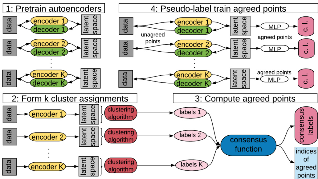
Fig. 1: The complete SPC method. (1) Pretrain auto encoders. (2) Perform multiple clustering s independently. (3) Identify agreed points as those that receive the same label in all ensemble members. (4) Perform pseudo-label training on agreed points and auto encoder training on unagreed points. Steps (2)–(4) are looped until the number of agreed points stops increasing.
图 1: 完整的SPC方法。(1) 预训练自动编码器。(2) 独立执行多次聚类。(3) 将获得所有集成成员相同标签的点识别为一致点。(4) 对一致点执行伪标签训练,对非一致点执行自动编码器训练。步骤(2)-(4)循环执行,直到一致点数量不再增加。
Training ends when the number of agreed points stops increasing. Then, each data point is assigned its most common cluster label across the (aligned) ensemble.
当达成一致的数据点数量不再增加时,训练结束。随后,每个数据点会被赋予其在(对齐后的)集成模型中最常见的聚类标签。
3.1 Formal Description
3.1 形式化描述
Given a dataset $\mathcal{X}\subseteq\mathbb{R}^{n}$ of size $N$ with $C$ true clusters, let $(f_{j}){1\leq j\leq K},f_{j}:\mathbb{R}^{n}\rightarrow$ $\mathbb{R}^{m}$ , and $(g_{j}){1\leq j\leq K},g_{j}:\mathbb{R}^{m}\rightarrow\mathbb{R}^{n}$ be the $K$ encoders and decoders, respectively. Let $\psi:\mathbb{R}^{N\times m}\rightarrow{0,\dots,C-1}^{N}$ be the clustering function, which takes the $N$ encoded data points as input, and returns a cluster label for each. We refer to the output of $\psi$ as a labelling. Let Γ : ${0,\ldots,C-1}^{K\times N}\to{0,\ldots,C-1}^{N}\times{0,1}^{N}$ be the consensus function, which aggregates $K$ different labellings of $\mathcal{X}$ into a single labelling, and also returns a Boolean vector indicating agreement. Then,
给定一个大小为 $N$ 的数据集 $\mathcal{X}\subseteq\mathbb{R}^{n}$,其中包含 $C$ 个真实簇。设 $(f_{j}){1\leq j\leq K},f_{j}:\mathbb{R}^{n}\rightarrow$ $\mathbb{R}^{m}$ 和 $(g_{j}){1\leq j\leq K},g_{j}:\mathbb{R}^{m}\rightarrow\mathbb{R}^{n}$ 分别为 $K$ 个编码器和解码器。定义聚类函数 $\psi:\mathbb{R}^{N\times m}\rightarrow{0,\dots,C-1}^{N}$,它以 $N$ 个编码后的数据点为输入,并为每个点返回一个簇标签。我们将 $\psi$ 的输出称为标记。设共识函数 Γ : ${0,\ldots,C-1}^{K\times N}\to{0,\ldots,C-1}^{N}\times{0,1}^{N}$ 将 $\mathcal{X}$ 的 $K$ 种不同标记聚合为单一标记,并返回一个表示一致性的布尔向量。
$$
(c_{1},\dots,c_{N}),(a_{1},\dots,a_{N})=\Gamma(\psi(f_{1}(\mathcal{X}))\circ\dots\circ\psi(f_{K}(\mathcal{X}))),
$$
$$
(c_{1},\dots,c_{N}),(a_{1},\dots,a_{N})=\Gamma(\psi(f_{1}(\mathcal{X}))\circ\dots\circ\psi(f_{K}(\mathcal{X}))),
$$
Algorithm 1 Training algorithm for SPC
算法 1 SPC训练算法
| for j = 1,..., K do Update parameters of f; and gj usingautoencoderreconstruction |
| endfor while number of agreed points increases do |
| compute e (c1,...,cv),(a1,...,an) as in (1) |
| for j =1,...,K do |
| Update parameters of f; and h, to minimize (2 |
| end for |
| endwhile |
where $(c_{1},\ldots,c_{N})$ are the consensus labels, and $a_{i}=1$ if the $i$ -th data point received the same cluster label (after alignment) in all labellings, and $0$ otherwise. The consensus function is the ensemble mode average, $c_{i}$ is the cluster label that was most commonly assigned to the $i$ -th data point.
其中 $(c_{1},\ldots,c_{N})$ 是共识标签,若第 $i$ 个数据点在所有标注(对齐后)中获得相同聚类标签则 $a_{i}=1$,否则为 $0$。共识函数采用集成众数平均法,$c_{i}$ 表示最常被分配给第 $i$ 个数据点的聚类标签。
Define $K$ pseudo-class if i ers $(h_{j}){1\leq j\leq K},h{j}:\mathbb{R}^{m}\rightarrow\mathbb{R}^{C}$ , and let
定义 $K$ 个伪分类器 $(h_{j}){1\leq j\leq K},h{j}:\mathbb{R}^{m}\rightarrow\mathbb{R}^{C}$,并设
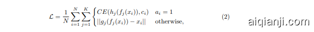
where $C E$ denotes categorical cross-entropy:
其中 $CE$ 表示分类交叉熵:
$$
\begin{array}{c}{{C E:\mathbb{R}^{C}\times{0,\dots,C-1}\to\mathbb{R}}}\ {{C E(x,n)=-\log(x[n]).}}\end{array}
$$
$$
\begin{array}{c}{{C E:\mathbb{R}^{C}\times{0,\dots,C-1}\to\mathbb{R}}}\ {{C E(x,n)=-\log(x[n]).}}\end{array}
$$
First, we pretrain the auto encoders, then compute $(c_{1},\dots,c_{N}),(a_{1},\dots,a_{N})$ and minimize $\mathcal{L}$ , recompute, and iterate until the number of agreed points stops increasing. The method is summarized in Algorithm 1.
首先,我们对自编码器进行预训练,然后计算 $(c_{1},\dots,c_{N}),(a_{1},\dots,a_{N})$ 并最小化 $\mathcal{L}$,重新计算并迭代,直到达成一致的点数停止增加。该方法总结在算法1中。
Figure 2 shows the training dynamics. Agreed points are those that receive the same cluster label in all members of the ensemble. As expected, the agreed points’ accuracy is higher than the accuracy on all points. Initially, the agreed points will not include those that are difficult to cluster correctly, such as an MNIST digit 3 that looks like a digit 5. Some ensemble members will cluster it as a 3 and others as a 5. The training process aims to make these difficult points into agreed points, thus increasing the fraction of agreed points, without decreasing the agreed points’ accuracy. Figure 2 shows that this aim is achieved. As more points become agreed (black dotted line), the total accuracy approaches the agreed accuracy. The agreed accuracy remains high, decreasing only very slightly (blue line). The result is that the total accuracy increases (orange line). We end training when the number of agreed points plateaus.
图 2: 展示了训练动态。达成共识点 (agreed points) 是指在集成所有成员中获得相同聚类标签的数据点。正如预期的那样,达成共识点的准确率高于所有数据点的准确率。最初,达成共识点不会包含那些难以正确聚类的数据点,例如看起来像数字5的MNIST数字3。一些集成成员会将其聚类为3,而另一些则聚类为5。训练过程旨在将这些困难点转化为达成共识点,从而增加达成共识点的比例,同时不降低其准确率。图2显示这一目标已经实现。随着越来越多的点达成共识(黑色虚线),总准确率逐渐接近达成共识准确率。达成共识准确率保持较高水平,仅略微下降(蓝线)。最终结果是总准确率上升(橙线)。当达成共识点数量趋于稳定时,我们终止训练。
3.2 Implementation Details
3.2 实现细节
Encoders are stacks of convolutional and batch norm layers; decoders of transpose convolutional layers. Decoders have a tanh activation on their output layer, all other layers use leaky ReLU. The MLP pseudo-classifier has a hidden layer of size 25. The latent space of the auto encoders has the size 50 for MNIST and Fashion M NIST, and 20 for smaller USPS. We inject noise from a multivariate normal into the latent space as a simple form of regular iz ation. As suggested in [48], the reconstruction loss is $\ell_{1}$ . The architectures are the same across the ensemble, diversity comes from random initialization and training dynamics.
编码器由卷积层和批量归一化层堆叠而成,解码器则由转置卷积层构成。解码器输出层采用tanh激活函数,其余层均使用Leaky ReLU。MLP伪分类器的隐藏层大小为25。自动编码器的潜空间维度在MNIST和Fashion MNIST中设为50,在较小的USPS数据集中设为20。我们向潜空间注入多元正态分布的噪声作为简单的正则化手段。如[48]所述,重建损失采用$\ell_{1}$。集成模型中所有架构保持相同,多样性来源于随机初始化和训练动态。
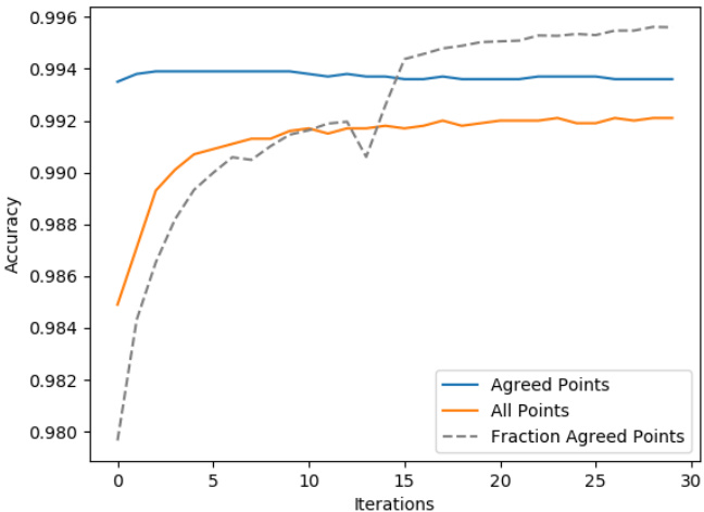
Fig. 2: Iterations of (2)–(4) in Figure 1 on MNIST.
图 2: MNIST数据集上对图1中(2)-(4)步骤的迭代过程
The clustering function ( $\psi$ above) is a composition of UMAP [32] and either HDBSCAN [31] or a Gaussian mixture model (GMM). As in previous works, we set the number of clusters to the ground truth. UMAP uses the parameters suggested in the clustering documentation clustering, n neighbours is 30 for MNIST and scaled in proportion to the dataset size for the others. HDBSCAN uses all default parameters. We cut the linkage tree at a level that gives the correct number of clusters. On the rare occasions when no such cut can be found, the clustering is excluded from the ensemble. The GMM uses all default parameters.
聚类函数(上述的$\psi$)是UMAP [32]与HDBSCAN [31]或高斯混合模型(GMM)的组合。如先前工作所示,我们将聚类数量设置为真实值。UMAP采用聚类文档建议的参数:MNIST数据集使用30个近邻,其他数据集按比例缩放。HDBSCAN采用全部默认参数。我们在连接树切割至获得正确聚类数量的层级。极少数情况下若无法找到合适切割点,则该聚类不纳入整体。GMM采用全部默认参数。
Consensus labels are taken as the most common across the ensemble, after alignment with the Hungarian algorithm (called the “direct” method in [3]).
共识标签采用集成中最常见的标签,经过与匈牙利算法对齐后确定(在[3]中称为"直接"方法)。
4 Proof of Correctness
4 正确性证明
Proving correctness requires proving that the expected accuracy of the agreed pseudo-labels is higher than that of all pseudo-labels, and that training with more accurate pseudo-labels makes the latent vectors easier to cluster correctly.
证明正确性需要证明达成一致的伪标签的预期准确率高于所有伪标签的准确率,并且使用更准确的伪标签进行训练会使潜在向量更容易正确聚类。
4.1 Agreed Pseudo-Labels are More Accurate
4.1 达成一致的伪标签更准确
Given that each member of the ensemble is initialized independently at random, and undergoes different stochastic training dynamics, we can assume that each cluster assignment contains some unique information. Formally, there is strictly positive conditional mutual information between any one assignment in the ensemble and the true cluster labels, conditioned on all the other assignments in the ensemble. From this assumption, the reasoning proceeds as follows.
由于集成中的每个成员都是随机独立初始化的,并且经历了不同的随机训练动态,我们可以假设每个聚类分配都包含一些独特信息。形式上,在给定集成中所有其他分配的条件下,集成中任一分配与真实聚类标签之间都存在严格正的条件互信息。基于这一假设,推理过程如下。
Choose an arbitrary data point $x_{0}$ and cluster $c_{0}$ . Let $X$ be a random variable (r.v.), indicating the true cluster of $x_{0}$ , given that $n$ members of the ensemble have assigned it to $c_{0}$ , and other assignments are unknown, $n\geq0$ . Thus, the event $X=c_{0}$ is the event that $x_{0}$ is correctly clustered. Let $Y$ be a Boolean r.v. indicating that the $(n+1)$ -th member of the ensemble also assigns it to $c_{0}$ . Assume that, if $n$ ensemble members have assigned $x_{0}$ to $c_{0}$ , and other assignments are unknown, then $x_{0}$ belongs to $c_{0}$ with probability at least $1/C$ and belongs to all other clusters with equal probability, i.e.,
选择一个任意数据点 $x_{0}$ 和聚类 $c_{0}$。设 $X$ 为随机变量 (r.v.),表示 $x_{0}$ 的真实聚类,已知集成中有 $n$ 个成员将其分配到 $c_{0}$,其他分配情况未知,且 $n\geq0$。因此,事件 $X=c_{0}$ 表示 $x_{0}$ 被正确聚类。设 $Y$ 为布尔随机变量,表示第 $(n+1)$ 个集成成员也将其分配到 $c_{0}$。假设当 $n$ 个集成成员将 $x_{0}$ 分配到 $c_{0}$ 且其他分配未知时,$x_{0}$ 属于 $c_{0}$ 的概率至少为 $1/C$,且属于其他所有聚类的概率均等,即
$$
\begin{array}{c}{{p(X=c_{0})=t}}\ {{\mathrm{}}}\ {{\forall c\neq c_{0},p(X=c)=(1-t)/(C-1),}}\end{array}
$$
$$
\begin{array}{c}{{p(X=c_{0})=t}}\ {{\mathrm{}}}\ {{\forall c\neq c_{0},p(X=c)=(1-t)/(C-1),}}\end{array}
$$
for some $1/C\leq t\leq1$ . It follows that the entropy $H(X)$ is a strictly decreasing function of $t$ (see appendix for proof). Thus, the above assumption on conditional mutual information, written $I(X;Y)>0$ , is equivalent to $p(X=c_{0}|Y)>$ $p(X=c_{0})$ . This establishes that the accuracy of the agreed labels is an increasing function of ensemble size. Standard pseudo-label training uses $n=1$ , whereas SPC uses $n>1$ and so results in more accurate pseudo-labels for training.
对于某些 $1/C\leq t\leq1$。由此可得熵 $H(X)$ 是关于 $t$ 的严格递减函数(证明见附录)。因此,上述关于条件互信息的假设 $I(X;Y)>0$ 等价于 $p(X=c_{0}|Y)>$ $p(X=c_{0})$。这表明约定标签的准确度是集成规模的递增函数。标准伪标签训练使用 $n=1$,而SPC采用 $n>1$,因此能生成更精确的训练用伪标签。
4.2 Increased Pseudo-Label Accuracy Improves Clustering
4.2 提升伪标签准确率改善聚类效果
Problem Formulation. Let $\mathcal{D}$ be a dataset of i.i.d. points from a distribution over $S\in\mathbb{R}^{n}$ , where $S$ contains $C$ true clusters $c_{1},\ldots,c_{C}$ . Let $T$ be the r.v.defined by the identity function on $S$ and $f:S\rightarrow\mathbb{R}^{m}$ , an encoding function para met rize d by $\theta$ , whose output is an r.v. $X$ . The task is to recover the true clusters conditional on $X$ , and we are interested in choosing $\theta$ such that this task is as easy as possible. Pseudo-label training applies a second function $h:\mathbb{R}^{m}\rightarrow{0,\ldots,C-1}$ and trains the composition $h\circ f:\mathbb{R}^{n}\rightarrow{0,\ldots,C-1}$ using gradient descent (g.d.), with cluster assignments as pseudo-labels. The claim is that an increased pseudo-label accuracy facilitates a better choice of $\theta$ .
问题表述。设 $\mathcal{D}$ 为从 $S\in\mathbb{R}^{n}$ 上的分布中独立同分布采样的数据集,其中 $S$ 包含 $C$ 个真实聚类 $c_{1},\ldots,c_{C}$。令 $T$ 为 $S$ 上恒等函数定义的随机变量,$f:S\rightarrow\mathbb{R}^{m}$ 是由参数 $\theta$ 参数化的编码函数,其输出为随机变量 $X$。任务是在给定 $X$ 的条件下恢复真实聚类,我们的目标是选择使该任务尽可能简化的 $\theta$。伪标签训练应用第二个函数 $h:\mathbb{R}^{m}\rightarrow{0,\ldots,C-1}$,并使用梯度下降 (g.d.) 训练复合函数 $h\circ f:\mathbb{R}^{n}\rightarrow{0,\ldots,C-1}$,其中聚类分配作为伪标签。核心论点是:伪标签准确率的提升有助于选择更优的 $\theta$。
To formalize “easy”, recall the definition of clustering as a partition that minimizes intra-cluster variance and maximizes inter-cluster variance. We want the same property to hold of the r.v. $X$ . Let $y:\mathcal{D}\rightarrow{0,\dots,C-1}$ be the true cluster assignment function and $Y$ the corresponding random variable, then ease of recovering the true clusters is captured by a high value of $d$ , where
为了形式化“容易”这一概念,回顾聚类的定义:即最小化簇内方差并最大化簇间方差的划分。我们希望随机变量 $X$ 也满足同样的性质。设 $y:\mathcal{D}\rightarrow{0,\dots,C-1}$ 为真实的簇分配函数,$Y$ 为对应的随机变量,那么恢复真实簇的难易程度由 $d$ 的高值所体现,其中
$$
d=\operatorname{Var}(\mathbb{E}[X|Y])-\mathbb{E}[\operatorname{Var}(X|Y)].
$$
$$
d=\operatorname{Var}(\mathbb{E}[X|Y])-\mathbb{E}[\operatorname{Var}(X|Y)].
$$
High $d$ means that a large fraction of the variance of $X$ is accounted for by cluster assignment, as, by Eve’s law, we can decompose:
高维 $d$ 意味着 $X$ 的方差大部分由聚类分配解释,根据 Eve 定律可分解为:
$$
\operatorname{Var}\left(X\right)=\operatorname{\mathbb{E}}[\operatorname{Var}(X|Y)]+\operatorname{Var}(\operatorname{\mathbb{E}}[X|Y]),
$$
$$
\operatorname{Var}\left(X\right)=\operatorname{\mathbb{E}}[\operatorname{Var}(X|Y)]+\operatorname{Var}(\operatorname{\mathbb{E}}[X|Y]),
$$
In the following, we assume that $f$ and $g$ are linear, $C=2$ , $h\circ f(\mathcal{D})\subseteq(0,1)$ , and $\mathbb{E}[T]={\vec{0}}$ . The proof proceeds by expressing the value of $d$ in terms of expected distances between encoded points after a training step with correct labels and with incorrect labels, and hence proving that the value is greater in the former case. We show that the expectation is greater in each coordinate, from which the claim follows by linearity (see appendix for details).
在下文中,我们假设$f$和$g$是线性的,$C=2$,$h\circ f(\mathcal{D})\subseteq(0,1)$,且$\mathbb{E}[T]={\vec{0}}$。证明过程通过用正确标签和错误标签训练步骤后编码点之间的期望距离来表达$d$的值,从而证明在前一种情况下该值更大。我们展示了在每个坐标上期望值更大,由此通过线性性得出命题成立(详见附录)。
Lemma 1. Let $x,x^{\prime}\in{\mathcal{D}}$ be two data points, and consider the expected squared distance between their encodings under $f$ . Let $u_{s a m e}$ and $u_{d i f}$ denote the value of this difference after a g.d. update in which both labels are the same and after $a$ step in which both labels are different, respectively. Then, $u_{s a m e}<u_{d i f f}$ .
引理1. 设 $x,x^{\prime}\in{\mathcal{D}}$ 为两个数据点,考虑它们在 $f$ 下编码的期望平方距离。设 $u_{same}$ 和 $u_{dif}$ 分别表示在梯度下降(g.d.)更新中两个标签相同时的差异值,以及两个标签不同时的差异值。则有 $u_{same}<u_{diff}$。
If $w\in\mathbb{R}^{m}$ and $w^{\prime}\in\mathbb{R}$ are, respectively, the vector of weights mapping the input to the $i$ -th coordinate of the latent space, and the scalar mapping the $i$ -th coordinate of the latent space to the output, then the expected squared distance in the $i$ -th coordinate of the latent vectors before the g.d. update is
如果 $w\in\mathbb{R}^{m}$ 和 $w^{\prime}\in\mathbb{R}$ 分别是将输入映射到潜在空间第 $i$ 个坐标的权重向量,以及将潜在空间第 $i$ 个坐标映射到输出的标量,那么在梯度下降更新前,潜在向量第 $i$ 个坐标的期望平方距离为
$$
\underset{x,x^{\prime}\sim T}{E}[(w^{T}x-w^{T}x^{\prime})^{2}]=\underset{x,x^{\prime}\sim T}{E}[(w^{T}(x-x^{\prime}))^{2}].
$$
$$
\underset{x,x^{\prime}\sim T}{E}[(w^{T}x-w^{T}x^{\prime})^{2}]=\underset{x,x^{\prime}\sim T}{E}[(w^{T}(x-x^{\prime}))^{2}].
$$
When the two labels are the same, assume w.l.o.g. that $y=y^{\prime}=0$ . Then, with step size $\eta$ , the update for $w$ and following expected squared difference $u_{s a m e}$ is
当两个标签相同时,不失一般性地假设 $y=y^{\prime}=0$。那么,在步长为 $\eta$ 的情况下,$w$ 的更新及随后的期望平方差 $u_{same}$ 为

When the two labels are different, assume w.l.o.g. that $y=0$ , $y^{\prime}=1$ , giving
当两个标签不同时,不失一般性地假设 $y=0$ , $y^{\prime}=1$ ,得到

It can then be shown (see appendix) that $u_{s a m e}<u_{d i f f}$ .
随后可以证明(见附录)$u_{s a m e}<u_{d i f f}$。
Lemma 2. Let $z$ be a third data point, $z\in{\mathcal{D}},z\neq x,x^{\prime}$ , and consider the expected squared distance of the encodings, under $f$ , of $x$ and $z$ . Let $v_{s a m e}$ and $v_{d i f}$ denote, respectively, the value of this difference after a g.d. update with two of the same labels, and with two different labels. Then, $v_{s a m e}=v_{d i f f}$ .
引理 2. 设 $z$ 为第三个数据点,$z\in{\mathcal{D}},z\neq x,x^{\prime}$,并考虑在编码函数 $f$ 下 $x$ 与 $z$ 的编码期望平方距离。令 $v_{same}$ 和 $v_{dif}$ 分别表示使用两个相同标签和两个不同标签进行梯度下降 (g.d.) 更新后的该距离值,则有 $v_{same}=v_{diff}$。
Lemma 3. Let s and $r$ denote, respectively, the expected squared distance between the encodings, under $f$ , of two points in the same cluster and between two points in different clusters. Then, there exist $\lambda_{1},\lambda_{2}>0$ whose values do not depend on the parameters of $f$ , such that $d=\lambda_{1}r-\lambda_{2}s$ .
引理3. 设s和$r$分别表示同一聚类内两点与不同聚类两点在$f$编码下的期望平方距离。则存在与$f$参数无关的$\lambda_{1},\lambda_{2}>0$,使得$d=\lambda_{1}r-\lambda_{2}s$成立。
For simplicity, assume that the clusters are equally sized. The argument can easily be generalized to clusters of arbitrary sizes. We then obtain
为简化起见,假设各集群大小相同。该论点可轻松推广至任意规模的集群。由此我们得出
$$
d={\frac{C-1}{2C}}r-{\frac{2C-1}{2C}}s,
$$
$$
d={\frac{C-1}{2C}}r-{\frac{2C-1}{2C}}s,
$$
where $C$ is the number of clusters (see appendix for proof).
其中 $C$ 为聚类数量(证明见附录)。
Definition 1. Let $\tilde{y}:\mathcal{D}\rightarrow{0,\dots,C-1}$ be the pseudo-label assignment function. For $d_{i},d_{j}\in{\mathcal{D}}$ , the pseudo-labels are pairwise correct iff $y(x_{i})=y(x_{j})$ and $\tilde{y}(x_{i})=\tilde{y}(x_{j})$ , or $y(x_{i})\neq y(x_{j})$ and $\tilde{y}(x_{i})\neq\tilde{y}(x_{j})$ .
定义 1. 设 $\tilde{y}:\mathcal{D}\rightarrow{0,\dots,C-1}$ 为伪标签分配函数。对于 $d_{i},d_{j}\in{\mathcal{D}}$,当且仅当 $y(x_{i})=y(x_{j})$ 且 $\tilde{y}(x_{i})=\tilde{y}(x_{j})$,或 $y(x_{i})\neq y(x_{j})$ 且 $\tilde{y}(x_{i})\neq\tilde{y}(x_{j})$ 时,伪标签成对正确。
Theorem 1. Let $d_{T}$ and $d_{F}$ denote, respectively, the value of d after a g.d. step from two pairwise correct labels and from two pairwise incorrect labels, and let $x,x^{\prime}\in{\mathcal{D}}$ as before. Then, $d_{T}>d_{F}$ .
定理1. 设$d_{T}$和$d_{F}$分别表示从两个成对正确标签和两个成对错误标签进行梯度下降(g.d.)步骤后的d值,且令$x,x^{\prime}\in{\mathcal{D}}$如前所述。则有$d_{T}>d_{F}$。
Proof. Let $r_{T},s_{T}$ , and $r_{F},s_{F}$ be, respectively, the values of $r$ and $s$ after a g.d. step from two pairwise correct labels and from two pairwise incorrect labels. Consider two cases. If $y(x)=y(x^{\prime})$ , then $r_{T}=r_{F}$ , by Lemma 2, and $s_{T}<s_{F}$ , by Lemmas 1 and 2, so by Lemma 3, $d_{T}>d_{F}$ . If $y(x)\neq y(x^{\prime})$ , then $s_{T}=s_{F}$ , by Lemma 2, and $r_{T}>r_{F}$ , by Lemmas 1 and 2, so again $d_{T}>d_{F}$ , by Lemma 3.
证明。设 $r_{T},s_{T}$ 和 $r_{F},s_{F}$ 分别为从两个成对正确标签和两个成对错误标签进行梯度下降 (g.d.) 步骤后的 $r$ 和 $s$ 值。考虑两种情况。若 $y(x)=y(x^{\prime})$ ,则根据引理2可得 $r_{T}=r_{F}$ ,而根据引理1和引理2有 $s_{T}<s_{F}$ ,因此由引理3可得 $d_{T}>d_{F}$ 。若 $y(x)\neq y(x^{\prime})$ ,则根据引理2有 $s_{T}=s_{F}$ ,根据引理1和引理2可得 $r_{T}>r_{F}$ ,故再次由引理3得出 $d_{T}>d_{F}$ 。
5 Experimental Results
5 实验结果
Following previous works, we measure accuracy and normalized mutual information (NMI). Accuracy is computed by aligning the predicted cluster labels with the ground-truth labels using the Hungarian algorithm [25] and then calculating as in the supervised case. NMI, as in [41], is defined as $2I(\tilde{Y};Y)/(H(\tilde{Y})+H(Y))$ , where $\tilde{Y}$ , $Y$ , $I(\cdot,\cdot)$ , and $H(\cdot)$ are, respectively, the cluster labels, ground truth labels, mutual information, and Shannon entropy. We report on two handwritten digits datasets, MNIST (size 70000) [26] and USPS (size 9298) [20], and FashionMNIST (size 70000) [42] of clothing items. Table 1 shows the central tendency for five runs and the best single run.
遵循先前的研究工作,我们采用准确率 (accuracy) 和归一化互信息 (normalized mutual information, NMI) 作为评估指标。准确率的计算方式是:首先使用匈牙利算法 [25] 将预测的聚类标签与真实标签对齐,然后按照监督学习场景下的方法进行计算。如文献 [41] 所述,NMI 定义为 $2I(\tilde{Y};Y)/(H(\tilde{Y})+H(Y))$,其中 $\tilde{Y}$、$Y$、$I(\cdot,\cdot)$ 和 $H(\cdot)$ 分别表示聚类标签、真实标签、互信息和香农熵。实验数据来自两个手写数字数据集 MNIST (规模 70000) [26] 和 USPS (规模 9298) [20],以及服装数据集 FashionMNIST (规模 70000) [42]。表 1 展示了五次运行的中心趋势指标及单次最佳运行结果。
We show results for two different clustering algorithms: Gaussian mixture model and the more advanced HDBSCAN [31]. Both perform similarly, showing robustness to clustering algorithm choice. SPC-GMM performs slightly worse on USPS and Fashion M NIST (though within margin of error), suggesting that HDBSCAN may cope better with the more complex images in Fashion M NIST and the smaller dataset in USPS. In Table 1, ‘SPC’ uses HDBSCAN.
我们展示了两种不同聚类算法的结果:高斯混合模型和更先进的HDBSCAN [31]。两者表现相似,表明对聚类算法选择具有鲁棒性。SPC-GMM在USPS和Fashion MNIST上表现略差(尽管在误差范围内),这表明HDBSCAN可能更适合处理Fashion MNIST中更复杂的图像和USPS中较小的数据集。在表1中,"SPC"使用的是HDBSCAN。
SPC (using either clustering algorithm) outperforms all existing approaches for both metrics on MNIST and USPS, and for NMI on Fashion M NIST. The disparity between the two metrics, and between HDBSCAN and GMM, on Fashion M NIST is due to the variance in cluster size. Many of the errors are lumped into one large cluster, and this hurts accuracy more than NMI, because being in this large cluster still conveys some information about what the ground truth cluster label is (see appendix for full details).
SPC (使用任一聚类算法) 在MNIST和USPS数据集的两个指标上均优于现有所有方法,在Fashion MNIST的NMI指标上也表现最佳。Fashion MNIST上两个指标的差异以及HDBSCAN与GMM之间的差异源于聚类规模的方差——大量错误被归入一个大型聚类,这对准确率的负面影响超过对NMI的影响,因为被归入该大聚类仍能传递部分真实类别标签的信息 (完整分析见附录)。
The most accurate existing methods use data augmentation. This is to be expected, given the well-established success of data augmentation in supervised learning [18]. More specifically, [17] have shown empirically that adding data augmentation to deep image clustering models improves performance in virtually all cases. Here, its effect is especially evident on the smaller dataset, USPS. For example, on MNIST, n2d [30] (which does not use data augmentation) is only 0.6 and 1.9 behind DDC [39], which does on ACC and NMI, respectively, but is 1.2 and 5.3 behind on USPS. SPC could easily be extended to include data augmentation, and even without using it, outperforms models that do.
现有最准确的方法采用数据增强技术。考虑到数据增强在监督学习[18]中已被证实的成功,这一结果在预期之中。具体而言,[17]通过实验证明,在几乎所有情况下,向深度图像聚类模型添加数据增强都能提升性能。在较小数据集USPS上,其效果尤为显著。例如在MNIST数据集上,未使用数据增强的n2d[30]在ACC和NMI指标上仅分别落后采用数据增强的DDC[39]0.6和1.9个点,但在USPS数据集上则落后1.2和5.3个点。SPC模型可轻松扩展以支持数据增强,且即便不使用该技术,其表现仍优于采用数据增强的模型。
Table 1: Accuracy and NMI of SPC compared to other top-performing image clustering models. The best results are in bold, and the second-best are emphasized. We report the mean and standard deviation (in parentheses) for five runs.
=uses data augmentation *=results taken from [34]
表 1: SPC与其他高性能图像聚类模型的准确率(ACC)和标准化互信息(NMI)对比。最优结果加粗显示,次优结果斜体标注。数据为五次运行的平均值及标准差(括号内)。
| MNIST | USPS | FashionMNIST | ||||
|---|---|---|---|---|---|---|
| ACC | NMI | ACC | NMI | ACC | NMI | |
| SPC-best | 99.21 | 97.49 | 98.44 | 95.44 | 67.94 | 73.48 |
| SPC SPC-GMM | 99.03 | 97.04 (.25) | 98.40 (.94) | 95.42 (.15) | 65.58 (2.09) | 72.09 (1.28) |
| DynAE[34] | 98.7 | 96.4 | 98.1 | 94.8 | 59.1 | 64.2 |
| ADC [33] | 98.6 | 96.1 | 98.1 | 94.8 | 58.6 | 66.2 |
| DDC [39] | 98.5 | 96.1 | 97.0 | 95.3 | 57.0 | 63.2 |
| n2d [30] | 97.9 | 94.2 | 95.8 | 90.0 | 67.2 | 68.4 |
| DLS [11] | 97.5 | 93.6 | - | - | 69.3 | 66.9 |
| JULE [45] | 96.4 | 91.3 | 95.0 | 91.3 | 56.3* | 60.8* |
| DEPICT [14] | 96.5 | 91.7 | 96.4 | 92.7 | 39.2* | 39.2* |
| DMSC [1] | 95.15 | 92.09 | 95.15 | 92.09 | - | - |
| ClusterGAN[35] | 95 | 89 | - | - | 63 | 64 |
| VADE [21] | 94.5 | 87.6* | 56.6* | 51.2* | 57.8* | 63.0* |
| IDEC [16] | 88.06 | 86.72 | 76.05 | 78.46 | 52.9* | 55.7* |
| CKM [13] | 85.4 | 81.4 | 72.1 | 70.7 | - | - |
| DEC [43] | 84.3 | 83.4* | 76.2* | 76.7* | 51.8* | 54.6* |
| DCN [44] | 83 | 81 | 68.8* | 68.3* | 50.1* | 55.8* |
*使用数据增强
*结果引自[34]
5.1 Ablation Studies
5.1 消融实验
Table 2 shows the effect of removing each component of our model. All settings use HDBSCAN. Particularly relevant are rows 2 and 3. As described in Section 3, we produce multiple labellings of the dataset and select for pseudo-label training only those data points that received the same label in all labellings. We perform two different ablations on this method: A1 and A2. Both use all data points for training, but A1 trains each ensemble on all data points using the labels computed in that ensemble member, and A2 uses the consensus labels. At inference, both use consensus labels. The significant drop in accuracy in both settings demonstrates that the strong performance of SPC is not just due to the application of an ensemble to existing methods, but rather to the novel method of label selection.
表 2 展示了移除模型各组件的影响。所有设置均采用 HDBSCAN。尤其关键的是第 2 和第 3 行。如第 3 节所述,我们生成数据集的多个标注版本,并仅选择在所有标注中具有相同标签的数据点进行伪标签训练。我们对该方法进行了两种不同的消融实验:A1 和 A2。两者都使用全部数据点进行训练,但 A1 使用各集成成员计算的标签在整个数据集上训练,而 A2 采用共识标签。在推理阶段,两者均使用共识标签。两种设置下准确率的显著下降表明,SPC 的优异性能不仅源于对现有方法的集成应用,更得益于标签选择的新颖方法。
It is interesting to observe that A1 performs worse than A2 on MNIST and USPS. Combining approximations in an ensemble has long been observed to give higher expected accuracy ([8,37,38,4]), so the training targets would be more accurate in A1 than in A2. We hypothesize that the reason that this fails to translate to improved clustering is a reduction in ensemble variance. On MNIST
有趣的是,观察到 A1 在 MNIST 和 USPS 上的表现比 A2 更差。长期以来,人们发现通过集成 (ensemble) 组合近似方法可以提高预期准确率 ([8,37,38,4]),因此 A1 的训练目标应该比 A2 更准确。我们假设这未能转化为聚类性能提升的原因是集成方差的降低。在 MNIST 上
| USPS | FashionMNIST | |||||||
|---|---|---|---|---|---|---|---|---|
| ACC | NMI | ACC | NMI | ACC | NMI | |||
| SPC99.03 | 3 (.1) 97.04 (.25) 98.40 (.94) 95.42 | 2 (.15) 65.58 (2.09) 72.09 (1.28) | ||||||
| A1 | 98.01 (.04) | 94.46 (.11) | 97.03 (.65) | 92.43 | (1.29) | 63.12 | (.16) | 70.59 (.01) |
| A2 | 98.18 (.05) | 94.86 6 (.09) | 97.31 (.89) | 92.99 (1.84) | 60.60 | (4.45) | 68.77 (.48) | |
| A3 | 98.02 2 (.19) | 94.45 5 (.43) | 95.85 | 5 (.80) 89.77 | (1.65) | 59.23 | 3 (3.58) | 67.09 9 (3.77) |
| A4 | 97.88 3 (.72) | 94.8 (.85) | 87.49 | 9 (7.93) | 82.68 (2.6) | 61.2 (4.28) | 67.28 3 (1.72) | |
| A5 | 96.17 (.26)9 | 91.07 (.23) | 87.00 (8.88) 80.79 | (7.43) | 55.29 (3.54) | 66.07 (1.04) | ||
| A6 | 70.24 | 77.42 | 70.46 | 71.11 | 42.08 | 49.22 |
Table 2: Ablation results, central tendency for three runs. A1=w/o label filtering; A2=w/o label sharing; A3=w/o ensemble; A4=pseudo-label training only; A5=UMAP+AE; A6=UMAP. Both A1 and A2 train on all data points. The former trains each member of the ensemble on their own labels, and the latter uses the consensus labels. A3 sets $K=1$ , in the notation of Section 3.1.
表 2: 消融实验结果,三次运行的中心趋势。A1=无标签过滤;A2=无标签共享;A3=无集成;A4=仅伪标签训练;A5=UMAP+AE;A6=UMAP。A1和A2均在所有数据点上训练。前者在集成中每个成员使用各自的标签训练,后者使用共识标签。A3在3.1节符号体系中设定$K=1$。
Table 3: Ablation studies on the size of the ensemble.
| MNIST | USPS | FashionMNIST |
|---|---|---|
| ACC | NMI | ACC |
| 25 98.48 | 95.60 | 97.70 |
| 20 98.49 | 95.64 | 97.87 |
| 15 99.03 (.10) | 97.04 (.25) | 98.40 (.94) |
| 12 98.82 | 96.54 | 98.20 |
| 10 98.78 | 96.42 | 98.39 |
| 8 98.75 | 96.32 | 98.41 |
| 6 98.61 | 95.90 | 98.40 |
| 5 98.56 | 95.82 | 98.30 |
| 4 98.47 | 95.60 | 98.27 |
| 3 98.44 | 95.50 | 98.15 |
| 2 98.27 | 95.07 | 97.98 |
| 1 98.02 (.19) | 94.45 (.43) | 95.85 (.80) |
表 3: 集成规模消融研究。
and USPS, high accuracy across the ensemble means high agreement. Giving the same training signal for every data point reduces variance further. Especially, compared with A2, the reduction is greatest on incorrectly clustered data points, because most incorrectly clustered data points are non-agreed points, and as argued in [23], high ensemble variance in the errors is important for performance.
在美国邮政服务(USPS)中,集成模型的高准确率意味着高一致性。为每个数据点提供相同的训练信号能进一步降低方差。特别是与A2相比,在错误聚类数据点上的方差降低最为显著,因为大多数错误聚类数据点都属于非一致点。如[23]所述,错误中较高的集成方差对性能至关重要。
A4 clusters in the latent space of one untrained encoder and then pseudo-label trains (essentially the method in [6]). It performs significantly worse than SPC, showing the value of the decoder, and of SPC’s label selection technique.
一个未经训练的编码器在潜在空间中的A4聚类,然后进行伪标签训练(本质上是[6]中的方法)。其表现明显逊于SPC,这证明了解码器的价值以及SPC标签选择技术的优势。
A3 omits the ensemble entirely. Comparing with A2 again shows that the ensemble itself only produces a small improvement. Alongside SPC’s label selection method, the improvement is much greater.
A3完全省略了集成方法。与A2再次比较表明,集成本身仅带来小幅提升。结合SPC的标签选择方法后,改进幅度显著增大。
5.2 Ensemble Size
5.2 集成规模
The number of auto encoders in the ensemble, $K$ in the terminology of Section 3.1, is a hyper parameter. We add the concatenation of all latent spaces as an additional element. Table 3 shows the performance for smaller ensemble sizes. In MNIST and USPS, where the variance is reasonably small, there is a discernible trend of the performance increasing with $K$ , then plateauing and starting to decrease. For Fashion M NIST, where the variance is higher, the pattern is less clear. For all three datasets, however, we can see a significant difference between an ensemble of size two and an ensemble of size one (i.e., no ensemble). We hypothesize that the decrease for $K=20,25$ is due to a decrease in the number of agreed points, and so fewer pseudo-labels to train the encoders.
集成中自动编码器的数量,即第3.1节中的超参数$K$。我们将所有潜在空间的拼接作为附加元素纳入考量。表3展示了较小集成规模下的性能表现。在方差相对较小的MNIST和USPS数据集上,可以观察到性能随$K$增加而提升的趋势,随后趋于平稳并开始下降。而对于方差较大的Fashion MNIST数据集,这种模式则不太明显。然而,在所有三个数据集中,都能明显观察到规模为二的集成与规模为一的集成(即无集成)之间存在显著差异。我们推测$K=20,25$时性能下降的原因是达成一致的样本点数量减少,从而导致用于训练编码器的伪标签数量减少。
6 Conclusion
6 结论
This paper has presented a deep clustering model, called selective pseudo-label clustering (SPC). SPC employs pseudo-label training, which alternates between clustering features extracted by a DNN, and treating these clusters as labels to train the DNN. We have improved this framework with a novel technique for preventing the DNN from learning noise. The method is formally sound and achieves a state-of-the-art performance on three popular image clustering datasets. Ablation studies have demonstrated that the high accuracy is not merely the result of applying an ensemble to existing techniques, but rather is due to SPC’s novel filtering method. Future work includes the application to other clustering domains, different from images, and an investigation of how SPC combines with existing deep clustering techniques.
本文提出了一种名为选择性伪标签聚类(SPC)的深度聚类模型。SPC采用伪标签训练方法,交替执行以下两个步骤:(1) 对深度神经网络(DNN)提取的特征进行聚类;(2) 将这些聚类结果作为标签来训练DNN。我们通过一种创新技术改进了该框架,可有效防止DNN学习噪声。该方法在理论上是严谨的,并在三个主流图像聚类数据集上实现了最先进的性能。消融实验表明,其高精度并非简单集成现有技术的结果,而是源于SPC创新的过滤方法。未来工作包括将该方法应用于图像以外的其他聚类领域,并研究SPC如何与现有深度聚类技术相结合。
Acknowledgments. This work was supported by the Alan Turing Institute under the UK EPSRC grant EP/N510129/1 and by the AXA Research Fund. We also acknowledge the use of the EPSRC-funded Tier 2 facility JADE (EP/P020275/1) and GPU computing support by Scan Computers International Ltd.
致谢。本研究由Alan Turing Institute在英国EPSRC资助(EP/N510129/1)和AXA Research Fund支持下完成。同时感谢EPSRC资助的Tier 2设施JADE(EP/P020275/1)以及Scan Computers International Ltd提供的GPU计算支持。
References
参考文献
7 Appendix A: Full Proofs
7 附录A: 完整证明
This appendix contains the full proofs of the results in Section 4.
本附录包含第4节结果的完整证明。
7.1 More Accurate Pseudo-Labels Supplement
7.1 更准确的伪标签补充
The only part omitted from the argument in the main paper is a proof for the claim about the entropy of the random variable $X$ . This is supplied by the following proposition.
主论文论证中唯一省略的部分是关于随机变量$X$熵的证明。以下命题提供了这一证明。
Proposition 1. Given a categorical random variable $X$ of the form
命题1. 给定一个形式为$X$的分类随机变量
$$
\begin{array}{c}{{p(X=c_{0})=t}}\ {{\forall c\neq c_{0},p(X=c)=\displaystyle\frac{1-t}{C-1},}}\end{array}
$$
$$
\begin{array}{c}{{p(X=c_{0})=t}}\ {{\forall c\neq c_{0},p(X=c)=\displaystyle\frac{1-t}{C-1},}}\end{array}
$$
for some $1/C\leq t\leq1$ , the entropy $H(X)$ is a strictly decreasing function of $t$ .
对于某些 $1/C\leq t\leq1$ ,熵 $H(X)$ 是关于 $t$ 的严格递减函数。
Proof.
证明。

The argument to the log is clearly an increasing function of $t$ for $t>1$ . Therefore, for $1/C\leq t<1$ , it is lower-bounded by setting $t=1/C$ . This gives
对数中的参数显然是 $t$ 在 $t>1$ 时的递增函数。因此,对于 $1/C\leq t<1$ 的情况,通过设 $t=1/C$ 可以得到其下界。由此可得
$$
\begin{array}{r l}&{\displaystyle\frac{d\left(H(X)\right)}{d t}\leq-2-\log\left(\frac{1/C}{1-1/C}(C-1)\right)}\ &{\quad\quad<-\log\left(\frac{1/C}{1-1/C}(C-1)\right)=-\log1=0.}\end{array}
$$
$$
\begin{array}{r l}&{\displaystyle\frac{d\left(H(X)\right)}{d t}\leq-2-\log\left(\frac{1/C}{1-1/C}(C-1)\right)}\ &{\quad\quad<-\log\left(\frac{1/C}{1-1/C}(C-1)\right)=-\log1=0.}\end{array}
$$
The derivative is always strictly negative with respect to $t$ , so, as a function of $t$ , $H(X)$ is always strictly decreasing.
关于 $t$ 的导数始终严格为负,因此作为 $t$ 的函数,$H(X)$ 始终严格递减。
7.2 Lemma 1 Supplement
7.2 引理1补充
The following is a proof for the claim that $u_{s a m e}<u_{d i f f}$ , as stated in Section 4.
以下是针对第4节中所述$u_{same}<u_{diff}$主张的证明。
Decomposing $u_{s a m e}$ according to the definition of variance (as the expectation of the square minus the square of the expectation) gives
根据方差定义(即平方的期望减去期望的平方)对$u_{same}$进行分解可得
$$
\begin{array}{r}{E_{x,x^{\prime}\sim T}[w^{T}(x-x^{\prime})-\eta w^{\prime}(||x||^{2}-||x^{\prime}||^{2})]^{2}+}\ {\mathrm{Var}(w^{T}(x-x^{\prime})-\eta w^{\prime}(||x||^{2}-||x^{\prime}||^{2})).}\end{array}
$$
$$
\begin{array}{r}{E_{x,x^{\prime}\sim T}[w^{T}(x-x^{\prime})-\eta w^{\prime}(||x||^{2}-||x^{\prime}||^{2})]^{2}+}\ {\mathrm{Var}(w^{T}(x-x^{\prime})-\eta w^{\prime}(||x||^{2}-||x^{\prime}||^{2})).}\end{array}
$$
The expectation term equals $0$ , as
期望项等于 $0$,因为
$$
\begin{array}{r}{w^{T}{\underset{x,x^{\prime}\sim T}{E}}[(x-x^{\prime})]-\eta w^{\prime}{\underset{x,x^{\prime}\sim T}{E}}[(||x||^{2}-||x^{\prime}||^{2})]=}\ {(w\mathbb{E}[T]-\mathbb{E}[T])-\eta w^{\prime}(\mathbb{E}[||T||^{2}]-\mathbb{E}[||T||^{2}])=0.}\end{array}
$$
$$
\begin{array}{r}{w^{T}{\underset{x,x^{\prime}\sim T}{E}}[(x-x^{\prime})]-\eta w^{\prime}{\underset{x,x^{\prime}\sim T}{E}}[(||x||^{2}-||x^{\prime}||^{2})]=}\ {(w\mathbb{E}[T]-\mathbb{E}[T])-\eta w^{\prime}(\mathbb{E}[||T||^{2}]-\mathbb{E}[||T||^{2}])=0.}\end{array}
$$
By symmetry, we can replace co variances involving $x^{\prime}$ with the same involving $x$ . The remaining term can then be rearranged to give
根据对称性,我们可以将涉及 $x^{\prime}$ 的协方差替换为涉及 $x$ 的相同项。剩余项可重新排列得到
$$
\begin{array}{c}{u_{s a m e}=2\mathrm{Var}(w^{T}x-\eta w^{\prime}||x||^{2})}\ {=2w^{T}C o v(T)w+2\eta w^{\prime}V a r(||x||^{2})-4\mathrm{Cov}(w^{T}x,\eta w^{\prime}||x||^{2}).}\end{array}
$$
$$
\begin{array}{c}{u_{s a m e}=2\mathrm{Var}(w^{T}x-\eta w^{\prime}||x||^{2})}\ {=2w^{T}C o v(T)w+2\eta w^{\prime}V a r(||x||^{2})-4\mathrm{Cov}(w^{T}x,\eta w^{\prime}||x||^{2}).}\end{array}
$$
Now rewrite $u_{d i f}$ . Decomposing as above gives
现在重写 $u_{d i f}$。按照上述方法分解可得
$$
\begin{array}{r l}&{\underset{x,x^{\prime}\sim T}{E}[w^{T}(x-x^{\prime})-\eta w^{\prime}(||x-x^{\prime}||^{2})]^{2}+}\ &{\quad\mathrm{Var}(w^{T}(x-x^{\prime})-\eta w^{\prime}(||x-x^{\prime}||^{2})),}\end{array}
$$
$$
\begin{array}{r l}&{\underset{x,x^{\prime}\sim T}{E}[w^{T}(x-x^{\prime})-\eta w^{\prime}(||x-x^{\prime}||^{2})]^{2}+}\ &{\quad\mathrm{Var}(w^{T}(x-x^{\prime})-\eta w^{\prime}(||x-x^{\prime}||^{2})),}\end{array}
$$
and here the expectation term does not equal 0:
这里的期望项不等于0:

The variance term can be expanded to give:
方差项可以展开为:
$$
\begin{array}{r l}&{\mathrm{Var}(w^{T}(x-x^{\prime})-\eta w^{\prime}(||x-x^{\prime}||^{2}))=}\ &{2w^{T}C o v(T)w+2\eta w^{\prime}\mathrm{Var}(||x-x^{\prime}||^{2})-}\ &{\quad\quad4\mathrm{Cov}(w^{T}x,\eta w^{\prime}||x-x^{\prime}||^{2}).}\end{array}
$$
$$
\begin{array}{r l}&{\mathrm{Var}(w^{T}(x-x^{\prime})-\eta w^{\prime}(||x-x^{\prime}||^{2}))=}\ &{2w^{T}C o v(T)w+2\eta w^{\prime}\mathrm{Var}(||x-x^{\prime}||^{2})-}\ &{\quad\quad4\mathrm{Cov}(w^{T}x,\eta w^{\prime}||x-x^{\prime}||^{2}).}\end{array}
$$
By comparing terms, we can see that this expression is at least as large as $u_{s a m e}$ . First, consider the covariance terms.
通过比较各项可以看出,该表达式至少与$u_{same}$同样大。首先考虑协方差项。


So, we see the covariance terms are equal.
因此,我们看到协方差项是相等的。
Next, compare the second variance terms
接下来,比较第二个方差项
$$
\begin{array}{r l}&{\quad\mathrm{Yar}(||x-x^{\prime}||^{2})}\ &{=\mathrm{Var}\left(\displaystyle\sum_{k=0}^{n\mathfrak{z}}(x)_{k}^{2}+(x^{\prime})_{k}^{2}-2(x)_{k}(x^{\prime})_{k}\right)}\ &{=\mathrm{Var}\left(\displaystyle\sum_{k=0}^{n\mathfrak{z}}(x)_{k}^{2}\right)+\mathrm{Var}\left(\displaystyle\sum_{k=0}^{n\mathfrak{z}}(x^{\prime})_{k}^{2}\right)+2\mathrm{Var}\left(\displaystyle\sum_{k=0}^{n\mathfrak{z}}x_{k}x_{k}^{\prime}\right)}\ &{=2\mathrm{Var}\left(\displaystyle\sum_{k=0}^{n\mathfrak{z}}(x)_{k}^{2}\right)+2\mathrm{Var}\left(\displaystyle\sum_{k=0}^{n\mathfrak{z}}x_{k}x_{k}^{\prime}\right)}\ &{=2(\mathrm{Var}(||x|^{2})+\mathrm{Var}(x^{\prime}x^{\prime}))}\ &{\geq\mathrm{Var}(||x|^{2}).}\end{array}
$$
$$
\begin{array}{r l}&{\quad\mathrm{Yar}(||x-x^{\prime}||^{2})}\ &{=\mathrm{Var}\left(\displaystyle\sum_{k=0}^{n\mathfrak{z}}(x)_{k}^{2}+(x^{\prime})_{k}^{2}-2(x)_{k}(x^{\prime})_{k}\right)}\ &{=\mathrm{Var}\left(\displaystyle\sum_{k=0}^{n\mathfrak{z}}(x)_{k}^{2}\right)+\mathrm{Var}\left(\displaystyle\sum_{k=0}^{n\mathfrak{z}}(x^{\prime})_{k}^{2}\right)+2\mathrm{Var}\left(\displaystyle\sum_{k=0}^{n\mathfrak{z}}x_{k}x_{k}^{\prime}\right)}\ &{=2\mathrm{Var}\left(\displaystyle\sum_{k=0}^{n\mathfrak{z}}(x)_{k}^{2}\right)+2\mathrm{Var}\left(\displaystyle\sum_{k=0}^{n\mathfrak{z}}x_{k}x_{k}^{\prime}\right)}\ &{=2(\mathrm{Var}(||x|^{2})+\mathrm{Var}(x^{\prime}x^{\prime}))}\ &{\geq\mathrm{Var}(||x|^{2}).}\end{array}
$$
Assuming that the data are not all identical, this implies that $u_{d i f}$ is strictly greater than $u_{s a m e}$ .
假设数据并非完全相同,这意味着$u_{d i f}$严格大于$u_{s a m e}$。
$$
\begin{array}{r l}&{u_{d\mathcal{G}}-u_{s\alpha\textbf{m}\ell}}\ &{=(\eta w^{\gamma})_{\textbf{z},\mathcal{F},\eta}^{2}[|x-x^{\prime}|]^{2}+2w^{\gamma}\mathrm{Cov}(T)w+}\ &{+2\eta w^{\gamma}\mathrm{St}\mathrm{Cl}|x-x^{\prime}|]^{2}-4\mathrm{Cov}(w^{\gamma}x,\eta w^{\prime}||x-x^{\prime}||^{2})-}\ &{-((2w^{\gamma}C\mathrm{ov}(T)w+2\eta w^{\gamma}V\mathrm{s}e T)|x|^{2})}\ &{-4\mathrm{Cov}(w^{\gamma}x,\eta w^{\prime}||x|^{2}))}\ &{=(\eta w^{\gamma})_{\textbf{z},\mathcal{F},\eta}^{2}[|x-x^{\prime}|^{2}]^{2}+}\ &{+2\eta w^{\gamma}\left(\mathrm{St}(|x-x^{\prime}||^{2})-\mathrm{Var}(|\mathfrak{z}|^{2})\right)-}\ &{-4\left(\mathrm{Cov}(w^{\gamma}x,\eta w^{\prime}||x-\mathfrak{z}||^{2})-\mathrm{Cov}(w^{\gamma}x,\eta w^{\prime}||x|^{2})\right)}\ &{=(\eta w^{\gamma})_{\textbf{z},\mathcal{F},\eta}^{2}[|x-x^{\prime}|^{2}]^{2}+}\ &{+2\eta w^{\gamma}\left(\mathrm{St}(|\mathfrak{z}-x^{\prime}||^{2})-\mathrm{Var}(|\mathfrak{z}|^{2})\right)}\ &{\geq(\eta w^{\gamma})_{\textbf{z},\mathcal{F},\eta}^{2}[|x-x^{\prime}|^{2}]^{2}\geq0.}\end{array}
$$
$$
\begin{array}{r l}&{u_{d\mathcal{G}}-u_{s\alpha\textbf{m}\ell}}\ &{=(\eta w^{\gamma})_{\textbf{z},\mathcal{F},\eta}^{2}[|x-x^{\prime}|]^{2}+2w^{\gamma}\mathrm{Cov}(T)w+}\ &{+2\eta w^{\gamma}\mathrm{St}\mathrm{Cl}|x-x^{\prime}|]^{2}-4\mathrm{Cov}(w^{\gamma}x,\eta w^{\prime}||x-x^{\prime}||^{2})-}\ &{-((2w^{\gamma}C\mathrm{ov}(T)w+2\eta w^{\gamma}V\mathrm{s}e T)|x|^{2})}\ &{-4\mathrm{Cov}(w^{\gamma}x,\eta w^{\prime}||x|^{2}))}\ &{=(\eta w^{\gamma})_{\textbf{z},\mathcal{F},\eta}^{2}[|x-x^{\prime}|^{2}]^{2}+}\ &{+2\eta w^{\gamma}\left(\mathrm{St}(|x-x^{\prime}||^{2})-\mathrm{Var}(|\mathfrak{z}|^{2})\right)-}\ &{-4\left(\mathrm{Cov}(w^{\gamma}x,\eta w^{\prime}||x-\mathfrak{z}||^{2})-\mathrm{Cov}(w^{\gamma}x,\eta w^{\prime}||x|^{2})\right)}\ &{=(\eta w^{\gamma})_{\textbf{z},\mathcal{F},\eta}^{2}[|x-x^{\prime}|^{2}]^{2}+}\ &{+2\eta w^{\gamma}\left(\mathrm{St}(|\mathfrak{z}-x^{\prime}||^{2})-\mathrm{Var}(|\mathfrak{z}|^{2})\right)}\ &{\geq(\eta w^{\gamma})_{\textbf{z},\mathcal{F},\eta}^{2}[|x-x^{\prime}|^{2}]^{2}\geq0.}\end{array}
$$
7.3 Lemma 2 Supplement
7.3 引理2补充
The following is the complete proof of Lemma 2, which was omitted from the main paper.
以下是引理2的完整证明,该证明在主论文中被省略。
Proof. vdiff − vsame
证明。vdiff − vsame

7.4 Lemma 3 Supplement
7.4 引理3补充
The following is the complete proof of Lemma 3, which was omitted from the main paper.
以下是引理3的完整证明,该证明在主论文中被省略。
Proof.
证明。
$$
\begin{array}{r l}&{\mathrm{Var}(T)=\displaystyle\frac{1}{2}\operatorname*{E}_{x,x^{\prime}\sim T}[(x-x^{\prime})^{2}]}\ &{\qquad=\displaystyle\frac{1}{2}\big(\operatorname*{\underset{x,x^{\prime}\sim T}{E}}[(x-x^{\prime})^{2}|y(x)=y(x^{\prime})|P(y(x)=y(x^{\prime}))+}\ &{\qquad\quad\operatorname*{\underset{x,x^{\prime}\sim T}{E}}[(x-x^{\prime})^{2}|y(x)\neq y(x^{\prime})|P(y(x)\neq y(x^{\prime}))}\ &{\qquad=\displaystyle\frac{1}{2}(s P(y(x)=y(x^{\prime}))+r P(y(x)\neq y(x^{\prime}))}\ &{\qquad=\displaystyle\frac{1}{2}\left(s\frac{1}{C}+r\frac{C-1}{C}\right).}\end{array}
$$
Noting that $s=2\mathbb{E}[\mathrm{Var}(T|C)]$ , and using Eve’s law, we have
注意到 $s=2\mathbb{E}[\mathrm{Var}(T|C)]$ ,并利用 Eve 定律,我们得到
$$
\begin{array}{l}{{d=\mathrm{Var}(T)-s}}\ {{\displaystyle~=\frac12\left(s\frac1C+r\frac{C-1}C\right)-s}}\ {{\displaystyle~=\frac{C-1}{2C}r-\frac{2C-1}{2C}s.}}\end{array}
$$
$$
\begin{array}{l}{{d=\mathrm{Var}(T)-s}}\ {{\displaystyle~=\frac12\left(s\frac1C+r\frac{C-1}C\right)-s}}\ {{\displaystyle~=\frac{C-1}{2C}r-\frac{2C-1}{2C}s.}}\end{array}
$$
7.5 Theorem 5 Supplement
7.5 定理5补充说明
The following is a more detailed version of the argument given in the main paper.
以下是主论文中论点的更详细版本。
If $y(x)=y(x^{\prime})$ , then Lemma 2 means that the expected distance of the encodings of $x$ and $x^{\prime}$ to any data point from another cluster is unchanged by whether the update was from points with the same or with different labels. Similarly, the distance between any two other points is unchanged by whether the update was from points with the same or with different labels. This establishes that $r_{T}=r_{F}$ . As for the intra-cluster variance, it is smaller after the update with the same labels than with different labels. Lemma 1 shows that the expected distance between the encodings of the two points themselves is smaller if the labels were the same, and the same argument as above shows that all other expected distances within clusters are unchanged.
如果 $y(x)=y(x^{\prime})$,那么引理2意味着,无论更新来自相同标签还是不同标签的点,$x$ 和 $x^{\prime}$ 的编码到其他簇中任意数据点的期望距离保持不变。类似地,任意其他两点之间的距离也不受更新标签是否相同的影响。由此可得 $r_{T}=r_{F}$。至于簇内方差,相同标签更新后的结果比不同标签更新后的更小。引理1表明,若标签相同,两点自身编码的期望距离会更小,而上述相同的论证表明簇内所有其他期望距离均未改变。
If $y(x)\neq y(x^{\prime})$ , then Lemma 2 means that the expected distance of the encodings of $x$ and any data point from the same cluster is unchanged by whether the update was from points with the same or with different labels (and the same for $x^{\prime}$ ). Similarly, the distance between any two other points is unchanged by whether the update was from points with the same or with different labels. This establishes that $s_{T}=s_{F}$ . As for the inter -cluster variance, it is larger after the update with the same labels than with different labels. Lemma 1 shows that the expected distance between the encodings of the two points themselves is larger if the labels were different, and the same argument as above shows that all other expected distances within clusters are unchanged.
如果 $y(x)\neq y(x^{\prime})$,那么引理2意味着,无论更新是来自具有相同标签还是不同标签的数据点,$x$ 和来自同一簇的任何数据点的编码期望距离保持不变(对于 $x^{\prime}$ 也是如此)。类似地,任何其他两点之间的距离也不受更新是否来自具有相同或不同标签的点的影响。这证明了 $s_{T}=s_{F}$。至于簇间方差,在更新后,使用相同标签的情况比使用不同标签的情况更大。引理1表明,如果标签不同,两个点本身的编码期望距离会更大,而上述相同的论点表明,簇内所有其他期望距离保持不变。
Table 4: Sizes of predicted clusters for MNIST.
| Zero | One | Two | Three | Four | Five | Six | Seven | Eight | Nine |
|---|---|---|---|---|---|---|---|---|---|
| HDBSCAN | 6923 | 7878 | 6979 | 7095 | 6802 | 6290 | 6911 | 7384 | 6776 |
| GMM | 6942 | 6958 | 6791 | 7885 | 6976 | 7096 | 7350 | 6294 | 6906 |
| Ground Truth | 7000 | 7000 | 7000 | 7000 | 7000 | 7000 | 7000 | 7000 | 7000 |
表 4: MNIST预测聚类大小。
Table 5: Sizes of predicted clusters for USPS.
表 5: USPS数据集的预测聚类大小
Table 6: Sizes of predicted clusters for Fashion M NIST.
表 6: Fashion MNIST 预测聚类大小
8 Appendix C: Extended Results
8 附录C: 扩展结果
The results in the main paper report the central tendency of five different training runs for each dataset. Tables 4, 5, and 6 show the sizes of the clusters predicted by SPC for one randomly selected run out of these five. On MNIST and USPS, where the accuracy of SPC is $>98%$ , the predicted sizes are close to the true sizes. On Fashion M NIST, where the accuracy is $\sim65%$ , there is a much greater variance. This accounts for the discrepancy in ACC and NMI for Fashion M NIST. Most of the errors are put into one large cluster, specifically the cluster that was aligned to ‘coat’ is over three times larger than it should be. This hurts accuracy more than NMI, because the incorrect data points in the ‘coat’ cluster count for zero when calculating the accuracy, but they are not randomly distributed among the other classes, so the conditional entropy of a data point that was mis-clustered as a coat is $<\log(10)$ . Actually, most of the mistakes in the ‘coat’ cluster are pullovers or shirts, and almost none of them are, for examples, boots or tops. Comparing the cluster sizes for SPC-HDBSCAN and SPC-GMM also accounts for the differences across ACC and NMI between these two settings on Fashion M NIST: SPC-GMM produces more uniformly-sized clusters, so the difference between ACC and NMI is smaller.
主论文中的结果报告了每个数据集五次不同训练运行的中心趋势。表4、表5和表6展示了SPC在这五次运行中随机选择的一次运行所预测的聚类大小。在MNIST和USPS数据集上,SPC的准确率>98%,预测大小接近真实大小。而在准确率~65%的Fashion MNIST上,方差则大得多。这解释了Fashion MNIST在ACC和NMI上的差异。大多数错误被归入一个大型聚类,特别是与"coat"对齐的聚类大小超出应有规模三倍以上。这对准确率的损害大于对NMI的影响,因为被错误归类到"coat"聚类的数据点在计算准确率时计为零,但它们并非随机分布于其他类别中,因此被误聚类为"coat"的数据点条件熵<$log(10)$。实际上,"coat"聚类中的错误大多是将套头衫或衬衫误判为外套,而几乎不会将靴子或上衣等误判其中。比较SPC-HDBSCAN和SPC-GMM的聚类大小也解释了这两种设置在Fashion MNIST上ACC和NMI的差异:SPC-GMM生成更均匀大小的聚类,因此ACC与NMI之间的差异较小。