SMPConv: Self-moving Point Representations for Continuous Convolution
SMPConv:连续卷积的自移动点表征
Abstract
摘要
Continuous convolution has recently gained prominence due to its ability to handle irregularly sampled data and model long-term dependency. Also, the promising experimental results of using large convolutional kernels have catalyzed the development of continuous convolution since they can construct large kernels very efficiently. Leveraging neural networks, more specifically multilayer perceptrons $(M L P s)$ , is by far the most prevalent approach to implementing continuous convolution. However, there are a few drawbacks, such as high computational costs, complex hyper parameter tuning, and limited descriptive power of filters. This paper suggests an alternative approach to building a continuous convolution without neural networks, resulting in more computationally efficient and improved performance. We present self-moving point representations where weight parameters freely move, and interpolation schemes are used to implement continuous functions. When applied to construct convolutional kernels, the experimental results have shown improved performance with drop-in replacement in the existing frameworks. Due to its lightweight structure, we are first to demonstrate the effectiveness of continuous convolution in a large-scale setting, e.g., ImageNet, presenting the improvements over the prior arts. Our code is available on https://github.com/sangnekim/SMPConv
连续卷积近来因其处理不规则采样数据和建模长期依赖的能力而备受关注。此外,大卷积核在实验中展现的优异表现进一步推动了连续卷积的发展,因为它们能高效构建大核结构。目前最主流的实现方式是利用神经网络(更具体而言是多层感知机 (MLPs)),但这种方法存在计算成本高、超参数调优复杂以及滤波器描述能力有限等缺陷。本文提出了一种无需神经网络的连续卷积构建方案,在提升计算效率的同时改进了性能。我们引入了自移动点表征技术,通过自由移动的权重参数和插值方案实现连续函数。当应用于构建卷积核时,实验表明该方案能在现有框架中即插即用地提升性能。得益于轻量化结构,我们首次在大规模场景(如ImageNet)中验证了连续卷积的有效性,其表现超越了现有技术。代码已开源:https://github.com/sangnekim/SMPConv
1. Introduction
1. 引言
There has been a recent surge of interest in representing the convolutional kernel as a function over a continuous input domain. It can easily handle irregularly sampled data both in time [1, 64] and space [67, 71], overcoming the drawbacks of the discrete convolution operating only on disc ret i zed sampled data with pre-defined resolutions and grids. With the progress in modeling and training continuous kernels, it has enjoyed great success in many practical scenarios, such as 3D point cloud classification and segmentation [40,45,57,63,70], image super resolution [62], object tracking [11], to name a few. Furthermore, the recent trends of using large convolutional kernels with strong empirical results urge us to develop a more efficient way to implement it [14,35], and the continuous convolution will be a promising candidate because of its capability to readily construct arbitrarily large receptive fields [48, 49].
近年来,将卷积核表示为连续输入域上的函数引起了广泛关注。这种方法能轻松处理时间和空间上的不规则采样数据 [1, 64][67, 71],克服了离散卷积仅能在预定义分辨率和网格的离散采样数据上运算的缺陷。随着连续核建模与训练技术的进步,该方法已在诸多实际场景中取得显著成功,例如3D点云分类与分割 [40,45,57,63,70]、图像超分辨率 [62]、目标跟踪 [11] 等。此外,当前使用大卷积核并取得强劲实证效果的趋势 [14,35],促使我们需要开发更高效的实现方式,而连续卷积因其能轻松构建任意大感受野的特性 [48, 49],将成为极具潜力的候选方案。
One of the dominant approaches to modeling the continuous kernel is to use a particular type of neural network architecture, taking as inputs low-dimensional input coordinates and generating the kernel values [48, 49], known as neural fields [42, 53] or simply MLPs. Using neural fields to represent the kernels, we can query kernel values at arbitrary resolutions in parallel and construct the large kernels with a fixed parameter budget, as opposed to the conventional discrete convolutions requiring more parameters to enlarge receptive fields. Thanks to recent advances to overcome the spectral bias on training neural fields [53], they can also represent functions with high-frequency components, which enables learned kernels to capture fine details of input data.
对连续核进行建模的主要方法之一是采用一种特定类型的神经网络架构,它以低维输入坐标作为输入并生成核值 [48, 49],这种方法被称为神经场 (neural fields) [42, 53] 或简称为 MLP。通过使用神经场来表示核,我们可以并行查询任意分辨率下的核值,并在固定参数预算下构建大核,这与传统离散卷积需要更多参数来扩大感受野形成对比。得益于近期克服神经场训练中频谱偏差的研究进展 [53],它们还能表示具有高频分量的函数,这使得学习到的核能够捕捉输入数据的精细细节。
While promising in various tasks and applications, this approach has a few downsides. First, it incurs considerable computational burdens to already computation-heavy processes of training deep neural networks. Each training iteration involves multiple forward and backward passes of MLPs to generate kernels and update the parameters of MLPs. This additional complexity prevents it from being applied to large-scale problems, such as ImageNet-scale, since it needs deeper and wider MLP architectures to construct more complex kernels with more input and output channels. Although MLPs can generate larger sizes and numbers of kernels without adding more parameters, it has been known that the size of MLPs mainly determines the complexity of the functions they represent and, eventually, the performance of the CNNs.
尽管在各种任务和应用中前景广阔,但这种方法存在一些缺点。首先,它给本就计算密集的深度神经网络训练过程带来了相当大的计算负担。每次训练迭代都涉及多层感知机 (MLP) 的多次前向和反向传播以生成卷积核并更新 MLP 参数。这种额外的复杂性使其难以应用于大规模问题(例如 ImageNet 级别),因为需要更深更宽的 MLP 架构来构建具有更多输入输出通道的复杂卷积核。虽然 MLP 无需增加参数就能生成更大尺寸和数量的卷积核,但众所周知,MLP 的规模主要决定了其所表征函数的复杂度,并最终影响 CNN 的性能。
Furthermore, the kernels generated by an MLP depend heavily on the architectural priors. As a universal function approx im at or, a neural network with sufficient depth and width can express any continuous functions [26]. However, we have empirically observed strong evidence that the architecture of neural networks has played a significant role in many practical settings, suggesting that various architectural changes to the kernel-generating MLPs would significantly affect the performance of CNNs. Considering a large number of hyper parameters in training neural networks, adding more knobs to tune, e.g., activation functions, width, depth, and many architectural variations of MLPs., would not be a pragmatic solution for both machine learning researchers and practitioners.
此外,由多层感知机 (MLP) 生成的核函数高度依赖于架构先验。作为通用函数逼近器,具备足够深度和宽度的神经网络能够表达任意连续函数 [26]。然而,我们通过实证观察到大量证据表明,神经网络架构在许多实际场景中起着关键作用,这意味着对核生成 MLP 进行各种架构调整会显著影响 CNN 的性能。考虑到训练神经网络涉及大量超参数,若额外增加可调节选项(如激活函数、宽度、深度以及 MLP 的多种架构变体),对机器学习研究者和实践者而言都非务实之选。
In this paper, we aim to build continuous convolution kernels with negligible computational cost and minimal archit ect ural priors. We propose to use moving point representations and implement infinite resolution by interpolating nearby moving points at arbitrary query locations. The moving points are the actual kernel parameters, and we connect the neighboring points to build continuous kernels. Recent techniques in neural fields literature inspire it, where they used grid or irregularly distributed points to represent features or quantities in questions (density or colors) for novel view synthesis [6, 54, 69, 72, 75]. The suggested approach only introduces minor computational costs (interpolation costs) and does not consist of neural networks (only point representations and interpolation kernels). Moreover, the spectral bias presented in training MLPs [47] does not exist in the suggested representation. Each point representation covers the local area of the input domain and is updated independently of each other, contrasted with MLPs, where updating each parameter would affect the entire input domain. Therefore, highly different values of nearby points can easily express high-frequency components of the function.
本文旨在构建计算成本可忽略且架构先验极少的连续卷积核。我们提出采用移动点表示法,通过在任意查询位置对邻近移动点进行插值来实现无限分辨率。移动点即为实际核参数,通过连接相邻点构建连续核函数。该方法受神经场领域近期技术启发[6, 54, 69, 72, 75],这些研究使用网格或不规则分布点来表示新视角合成中的特征或目标量(如密度或颜色)。所提方案仅引入微小计算成本(插值开销),且不包含神经网络(仅有点表示和插值核)。此外,多层感知器(MLP)训练中存在的频谱偏差[47]在该表示中并不存在。每个点表示覆盖输入域的局部区域,且更新过程相互独立——这与MLP形成鲜明对比,后者参数更新会影响整个输入域。因此,邻近点的高度差异化取值可轻松表达函数的高频分量。
The proposed method can also be more parameter efficient than the discrete convolution to construct the large kernels. Depending on the complexity of the kernels to be learned, a few numbers of points may be sufficient to cover a large receptive field (e.g., a unimodal function can be approximated by a single point). Many works have extensively exploited non-full ranks of the learned kernels to implement efficient convolutions or compress the models [35]. Our approach can likewise benefit from the pres- ence of learned kernels with low-frequency components.
所提方法在构建大卷积核时也能比离散卷积更节省参数量。根据待学习卷积核的复杂度,少量采样点可能就足以覆盖大感受野(例如,单峰函数可用单个点近似)。已有许多工作广泛利用学习卷积核的非满秩特性来实现高效卷积或模型压缩 [35]。我们的方法同样能受益于学习到的低频成分卷积核。
We conduct comprehensive experimental results to show the effectiveness of the proposed method. First, we demonstrate that moving point representations can approximate continuous functions very well in 1D and 2D function fitting experiments. Then, we test its ability to handle longterm dependencies on various sequential datasets. Finally, we also evaluate our model on 2D image data. Especially, we perform large-scale experiments on the ImageNet classification dataset (to our knowledge, it is the first attempt to use continuous convolution for such a large-scale problem). Our proposed method can be used as a drop-in replacement of convolution layers for all the above tasks without bells and whistles. The experimental results show that it consistently improves the performance of the prior arts.
我们通过全面的实验结果验证了所提方法的有效性。首先,在一维和二维函数拟合实验中证明移动点表示能很好地逼近连续函数。其次,在多个序列数据集上测试了其处理长期依赖关系的能力。最后,还在二维图像数据上评估了模型性能,特别是在ImageNet分类数据集上进行了大规模实验(据我们所知,这是首次将连续卷积应用于如此大规模的问题)。该方法无需任何修饰即可作为卷积层的即插即用替代方案,实验结果表明其性能始终优于现有技术。
2. Related works
2. 相关工作
Neural fields and continuous convolution. Neural fields have recently emerged as an alternative neural network representation [53]. It is a field parameterized by a neural network, such as simple MLP, taking as lowdimensional coordinates input and generating quantity in questions. It has shown great success in various visual computing domains, such as novel view synthesis [42], 3D shape representation [41, 44], and data compression [18], to name a few. Since it is a function over a continuous input domain, it can produce outputs at arbitrary resolutions. Recent studies have exploited its continuous nature to model continuous kernels for CNNs [48, 49, 63]. [63] used an MLP architecture to implement the continuous kernel to handle irregularly sampled data, such as 3D point clouds. While successful, the descriptive power of the learned kernel is limited due to its bias toward learning low-frequency components. With the recent advances in overcoming the spectral bias [53], [49] has explored various activation functions to improve the performance of CNNs. To further im- prove, [48] proposed to learn the receptive field sizes and showed impressive performance on multiple tasks.
神经场与连续卷积。神经场近年来作为一种替代性神经网络表征崭露头角 [53]。它是由神经网络(如简单MLP)参数化的场,接收低维坐标输入并生成目标量值。该技术在多个视觉计算领域展现出卓越成效,包括新视角合成 [42]、3D形状表征 [41,44] 以及数据压缩 [18] 等。由于其在连续输入域上定义,可生成任意分辨率的输出。最新研究利用其连续性特性为CNN建模连续卷积核 [48,49,63]。[63] 采用MLP架构实现连续核来处理不规则采样数据(如3D点云),但所学卷积核因偏向低频成分而导致表征能力受限。随着克服频谱偏差 [53] 的技术进步,[49] 探索了多种激活函数来提升CNN性能。[48] 进一步提出学习感受野大小的方法,在多项任务中展现出优异表现。
We also propose a method that can likewise be classified as a neural field. However, we implement a field without neural networks, using self-moving point representations and interpolation schemes. It significantly reduces the computational costs to compute the kernels during training compared to the conventional MLP-based methods. Furthermore, it removes the burden of numerous hyperparameter searches for a newly introduced neural network in the already complicated training procedure.
我们还提出了一种同样可归类为神经场 (neural field) 的方法。但不同于传统基于MLP的方法,我们采用自移动点表示和插值方案实现了无需神经网络的场表示。相比传统方法,该方法显著降低了训练期间计算核函数的计算成本,同时避免了在已复杂的训练流程中为新引入神经网络进行大量超参数搜索的负担。
Grid and point representations. Although MLP-based neural fields have succeeded in many tasks, they require substantial computational costs for training and inference, and the spectral bias presented in MLPs often degrades the performance. In order to reduce the computations and avoid the issues of using MLPs, classical grid-based representations have been adopted in the neural fields. Plenoxels [72] stores the coefficients of spherical harmonic in the 3D voxel structure and implements the infinite resolution via the inter pol ation methods, reducing the training time from days to minutes. Instant-NGP [43] further optimized the speed using a hash-based indexing algorithm. The combination of grid representations and MLPs has been extensively explored to find better solutions [6, 54].
网格与点表示法。尽管基于MLP的神经场已在众多任务中取得成功,但其训练和推理过程需要高昂的计算成本,且MLP固有的频谱偏差常导致性能下降。为降低计算量并规避MLP的缺陷,神经场领域重新采用了传统的基于网格的表示方法。Plenoxels [72] 将球谐系数存储在三维体素结构中,并通过插值方法实现无限分辨率,将训练时间从数天缩短至分钟级。Instant-NGP [43] 进一步采用基于哈希的索引算法优化了速度。学界已广泛探索网格表示与MLP的混合架构以寻求更优方案 [6, 54]。
Point representations have been recently suggested in neural fields to improve the shortcomings in grid-based representations, thanks to their flexibility and express i bility [69, 75]. They can generate outputs over a continuous input domain by interpolating neighboring points given a query point. It can be more accurate and parameter efficient than the grid-based ones since it can adaptively locate points, considering the complexity of functions, e.g., fewer points in low-frequency areas. Although our work is largely inspired by these works, 1. we repurpose the point representations to build continuous convolutional kernels, 2. we do not use MLPs that would introduce additional modeling complexity, 3. our method does not require complex initializations (or algorithms) to relocate points, such as depthbased initialization [69] and mask-based initialization [75].
点表征 (point representations) 最近在神经场 (neural fields) 中被提出,以改善基于网格表征的缺陷,这得益于其灵活性和表达能力 [69, 75]。它们可以通过在给定查询点时插值邻近点,在连续输入域上生成输出。由于它能根据函数的复杂性(例如在低频区域使用较少的点)自适应地定位点,因此比基于网格的表征更准确且参数效率更高。尽管我们的工作很大程度上受到这些研究的启发,但 1. 我们重新利用点表征来构建连续卷积核,2. 我们不使用会增加额外建模复杂度的多层感知机 (MLP),3. 我们的方法不需要复杂的初始化(或算法)来重新定位点,例如基于深度的初始化 [69] 和基于掩码的初始化 [75]。
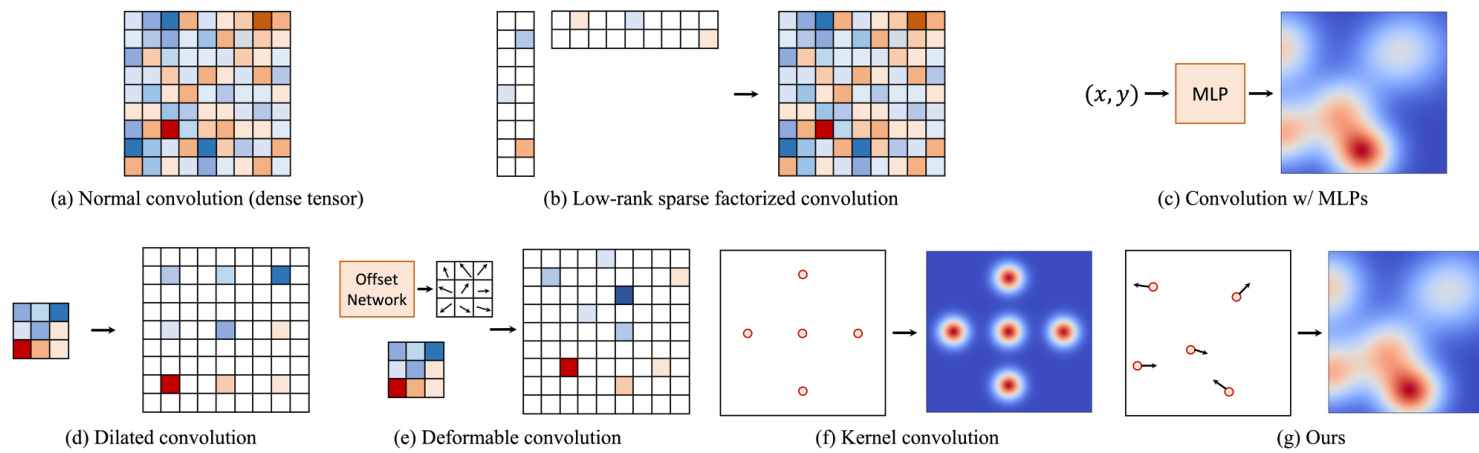
Figure 1. A various methods for large kernel construction.
图 1: 大卷积核构建的多种方法
Large kernel convolution. Since the great success of VGG-style CNNs [25, 27, 52, 56] in ImageNet [13], we repeatedly apply small kernels (e.g., $3\times3$ kernel) with deep layers to get a large receptive field and deal with long-term dependencies. With the massive success of transformers in the vision domain [16,17,37,60], which have a large receptive field, recent studies have started to revisit the descriptive power of large kernels [14, 35, 38, 58]. RepLKNet [14] has shown we can increase the kernel size up to $31\times31$ with the help of the re parameter iz ation trick. More recently, SLaK [35] managed to scale the kernel size to $51\times51$ and $61\times61$ , showing improved performance with dynamic sparsity and low-rank factorization (Fig. 1-(b)). While promising, the number of parameters increases according to the kernel size, which is a major bottleneck in representing large kernels.
大核卷积。自VGG风格的CNN [25, 27, 52, 56]在ImageNet [13]上取得巨大成功以来,我们通过重复应用小核(例如 $3\times3$ 核)配合深层网络来获得大感受野并处理长程依赖关系。随着Transformer [16,17,37,60]在视觉领域因其大感受野特性获得巨大成功,近期研究开始重新审视大核的描述能力 [14, 35, 38, 58]。RepLKNet [14]证明借助重参数化技巧可将核尺寸增大至 $31\times31$。最新研究SLaK [35]更将核尺寸扩展至 $51\times51$ 和 $61\times61$,通过动态稀疏性与低秩分解(图1-(b))展示了性能提升。尽管前景可观,参数量会随核尺寸增大而增加,这成为表征大核的主要瓶颈。
The continuous kernel can construct large kernels with a fixed parameter budget (Fig. 1-(c)). CKConv [49] and Flex- Conv [48] have exploited this property and demonstrated that their method can model long-term dependencies by constructing large kernels on various datasets. However, they introduce a considerable amount of computations to the training process, and they have yet to perform largescale experiments, e.g., ImageNet. To the best of our knowledge, our approach is the first to conduct such a large-scale experiment using continuous convolution.
连续卷积核能够在固定参数预算下构建大尺寸核 (图 1-(c))。CKConv [49] 和 Flex-Conv [48] 利用这一特性,通过在不同数据集上构建大尺寸核证明了其方法对长程依赖关系的建模能力。然而,这些方法会显著增加训练过程的计算量,且尚未进行大规模实验 (例如 ImageNet)。据我们所知,本研究是首个使用连续卷积进行如此大规模实验的工作。
On the other hand, dilated convolutions [7, 8] can also be used to enlarge receptive fields with a small number of parameters, and they also do not introduce additional computations during training (Fig. 1-(d)). Deformable convolutions [10] look similar to ours in terms of moving points arbitrarily (Fig. 1-(e)). However, they learn how to deform the kernels (or predict the offset) during inference. On the other hand, we adjust the locations of the point representations during training to find the optimal large kernels. A concurrent work suggests learning the offsets during training [24]. In contrast to ours, it is a discrete formulation, thus losing the benefits of continuous convolution. Furthermore, we adjust the receptive fields of each point representation separately, yielding more expressive representations.
另一方面,空洞卷积 (dilated convolution) [7, 8] 也能用较少参数扩大感受野,且不会在训练时引入额外计算 (图 1-(d))。可变形卷积 (deformable convolution) [10] 在任意移动点位的特性上与我们的方法类似 (图 1-(e)),但其在推理时学习如何变形卷积核 (或预测偏移量)。而我们的方法通过在训练时调整点位表征的位置来寻找最优大卷积核。一项同期研究提出在训练时学习偏移量 [24],但与我们的连续卷积形式不同,其采用离散表述因而丧失了连续卷积的优势。此外,我们单独调整每个点位表征的感受野,从而获得更具表现力的表征。
Continuous convolution for point clouds. There have been many continuous convolution approaches to handle 3D point cloud data, which is an important example of irregularly sampled data. PointNet [45] and PointNe $^{++}$ [46] are pioneer works that use average pooling and $1\times1$ convolution to aggregate features. [34, 36, 63, 66] leveraged MLPs to implement continuous convolution. KPConv [57] is also considered a continuous convolution and shares some similarities with ours (Fig. 1-f). They also used point representation and interpolation kernels for handling point clouds. However, their points are fixed over the training, unlike ours. They also proposed a deformable version, which requires additional neural networks to predict the offset of the kernel points.
点云的连续卷积。已有多种连续卷积方法用于处理3D点云数据,这是不规则采样数据的重要实例。PointNet [45] 和 PointNe$^{++}$ [46] 是开创性工作,使用平均池化和$1\times1$卷积来聚合特征。[34, 36, 63, 66] 利用多层感知机 (MLP) 实现连续卷积。KPConv [57] 也被视为连续卷积,与我们的方法存在相似之处 (图 1-f)。该方法同样采用点表示和插值核来处理点云,但其核点位置在训练过程中固定,而我们的方法则不同。他们还提出了可变形版本,需要通过额外神经网络预测核点偏移量。
3. SMPConv
3. SMPConv
3.1. Self-moving point representation
3.1. 自移动点表示
This section describes the proposed self-moving point representation to represent a continuous function. Let $d$ be the size of the input coordinates dimension, e.g., 1 in timeseries data and 2 in the spatial domain. SMP : Rd → RNc is a vector-valued function, mapping from the input coordinates to the output kernel vectors, where $N_{c}$ is a channel size. Given a query point $x\in\mathbb{R}^{d}$ , we define a continuous
本节介绍所提出的自移动点表示法,用于表示连续函数。设 $d$ 为输入坐标维度的大小,例如时间序列数据中为1,空间域中为2。SMP: Rd → RNc 是一个向量值函数,将输入坐标映射到输出核向量,其中 $N_{c}$ 是通道大小。给定一个查询点 $x\in\mathbb{R}^{d}$,我们定义一个连续的
kernel function as follows.
核函数如下。
$$
\mathrm{SMP}(x;\phi)=\frac{1}{|\mathcal{N}(x)|}\sum_{i\in\mathcal{N}(x)}g(x,p_{i},r_{i})w_{i},
$$
$$
\mathrm{SMP}(x;\phi)=\frac{1}{|\mathcal{N}(x)|}\sum_{i\in\mathcal{N}(x)}g(x,p_{i},r_{i})w_{i},
$$
where $\boldsymbol{\phi}={{p_{i}}_{i=1}^{N_{p}},{w_{i}}_{i=1}^{N_{p}},{r_{i}}_{i=1}^{N_{p}}}$ is a set of learn- able parameters, and $N_{p}$ is the number of points that are used to represent the function. $p_{i}\in\mathbb{R}^{d}$ is the coordinates of self-moving point representation $w_{i}\in\mathbb{R}^{N_{c}}$ , and each point representation also has a learnable radius, $r_{i}\in\mathbb{R}^{+}$ is a positive real number, which we implement it by clipping for numerical stability. We define a distance function $\dot{\boldsymbol g}:\dot{\mathbb R}^{d}\times\mathbb R^{d}\times\mathbb R^{+}\to\mathbb R$ as follows,
其中 $\boldsymbol{\phi}={{p_{i}}_{i=1}^{N_{p}},{w_{i}}_{i=1}^{N_{p}},{r_{i}}_{i=1}^{N_{p}}}$ 是一组可学习参数,$N_{p}$ 是用于表示函数的点数。$p_{i}\in\mathbb{R}^{d}$ 是自移动点表示的坐标,$w_{i}\in\mathbb{R}^{N_{c}}$,每个点表示还有一个可学习的半径,$r_{i}\in\mathbb{R}^{+}$ 是一个正实数,出于数值稳定性考虑我们通过裁剪实现。我们定义一个距离函数 $\dot{\boldsymbol g}:\dot{\mathbb R}^{d}\times\mathbb R^{d}\times\mathbb R^{+}\to\mathbb R$ 如下:
$$
g(x,p_{i},r_{i})=1-\frac{|x-p_{i}|{1}}{r{i}},
$$
$$
g(x,p_{i},r_{i})=1-\frac{|x-p_{i}|{1}}{r{i}},
$$
where $|\cdot|{1}$ is a L1 distance. $\mathcal{N}(x)$ is a set of indices of neighboring points of a query coordinate $x$ , defined as ${\mathcal{N}}(x)={i|g(x,p{i},r_{i})>0,\forall i}$ . Thus, points beyond a certain distance (depending on the radius) will not affect the query point. Hence, SMP generates output vectors by a weighted average of the nearby point representations. Note that all three parameters ${p_{i}},{w_{i}},{r_{i}}$ are jointly trained with the CNN model parameters, and the gradients w.r.t those parameters can be easily computed using an automatic differentiation library. As the name SMP suggests, the coordinates ${p_{i}}$ are updated during training, resulting in moving points representation.
其中 $|\cdot|{1}$ 是 L1 距离。$\mathcal{N}(x)$ 是查询坐标 $x$ 的邻近点索引集合,定义为 ${\mathcal{N}}(x)={i|g(x,p{i},r_{i})>0,\forall i}$。因此,超出特定距离(取决于半径)的点不会影响查询点。于是,SMP 通过邻近点表示的加权平均生成输出向量。注意,所有三个参数 ${p_{i}},{w_{i}},{r_{i}}$ 都与 CNN 模型参数联合训练,且这些参数的梯度可通过自动微分库轻松计算。正如 SMP 名称所示,坐标 ${p_{i}}$ 在训练过程中会更新,从而形成移动点表示。
Compared to a fixed-point representation, where ${p_{i}}$ are not trainable, ours can approximate complex functions more precisely. Since each point can move freely, more points can be gathered in high-frequency areas. On the other hand, few points can easily represent low-frequency components, resulting in more parameter-efficient representation. For example, a single point may be sufficient to approximate unimodal functions.
与定点表示法(其中${p_{i}}$不可训练)相比,我们的方法能更精确地逼近复杂函数。由于每个点可自由移动,更多点能聚集在高频区域。另一方面,少量点即可轻松表示低频分量,从而实现更高参数效率的表示。例如,单个点可能足以逼近单峰函数。
3.2. SMPConv
3.2. SMPConv
We leverage the suggested representation to implement a continuous convolution operator. In one dimensional case, $d=1$ , a continuous convolution can be formulated as,
我们利用所提出的表示方法实现了一个连续卷积算子。在一维情况下($d=1$),连续卷积可以表示为:
$$
\big(f\ast\mathrm{SMP}\big)(x)=\sum_{c=1}^{N_{c}}\int_{\mathbb{R}}f_{c}(\tau)\mathrm{SMP}_{c}(x-\tau)d\tau,
$$
$$
\big(f\ast\mathrm{SMP}\big)(x)=\sum_{c=1}^{N_{c}}\int_{\mathbb{R}}f_{c}(\tau)\mathrm{SMP}_{c}(x-\tau)d\tau,
$$
where $f:\mathbb{R}\to\mathbb{R}^{N_{c}}$ is a input function and the $f_{c}$ and $\operatorname{SMP}{c}$ denote the $c$ -th element of the inputs. The convolution operator generates a function, computing the filter responses by summing over entire $N_{c}$ channels. One SMP representation corresponds a convolution operator, and multiple SMPs are used to implement one convolutional layer to generate multiple output channels. In contrast to the previous MLPbased continuous convolution, which uses one neural network for one convolutional layer, our approach has separate parameters for each convolution filter in a layer. It gives more freedom to each filter and results in more descriptive power of the learned filter.
其中 $f:\mathbb{R}\to\mathbb{R}^{N_{c}}$ 是输入函数,$f_{c}$ 和 $\operatorname{SMP}{c}$ 表示输入的第 $c$ 个元素。卷积算子生成一个函数,通过对所有 $N_{c}$ 个通道求和来计算滤波器响应。一个SMP表示对应一个卷积算子,多个SMP用于实现一个卷积层以生成多个输出通道。与之前基于MLP的连续卷积(每个卷积层使用一个神经网络)相比,我们的方法为层中的每个卷积滤波器设置了独立参数。这为每个滤波器提供了更大自由度,从而增强了所学滤波器的描述能力。
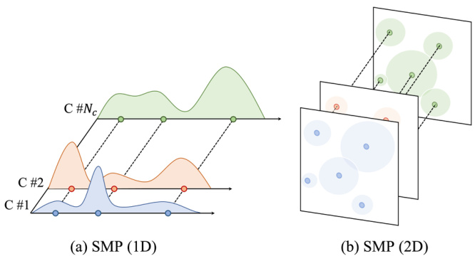
Figure 2. Self-moving point representation. (a) SMP as a function of the one-dimensional input domain, and (b) SMP as a function of the two-dimensional input domain. ‘C #1’ means the first channel. Each channel shares the location of the points, whereas each channel has its own weight parameters.
图 2: 自移动点表示。(a) 一维输入域下的 SMP 函数,(b) 二维输入域下的 SMP 函数。"C #1"表示第一通道。各通道共享点位置,但每个通道拥有独立的权重参数。
As depicted in Fig. 2, the kernels of each filter share the position parameters. That is, each filter of one layer has its own position parameters. Although we could use different SMP for different channels. However, it will considerably increase the number of learnable parameters $\it{{p_{i}}}$ per channel), and we believe that locating points at the same location for a convolutional filter can be a reasonable prior, where a convolutional filter can focus on specific areas in the input domain.
如图 2 所示,每个滤波器的核共享位置参数。也就是说,每一层的每个滤波器都有自己独立的位置参数。尽管我们可以为不同通道使用不同的 SMP (Spatial Modulation Parameters),但这会显著增加每个通道的可学习参数量 $\it{{p_{i}}}$。我们认为,让卷积滤波器的定位点保持相同位置是一种合理的先验设定,这样卷积滤波器可以专注于输入域中的特定区域。
We leverage our continuous formulation to construct large kernels, motivated by the recent success of using them in many tasks. We can create arbitrary size large kernels by querying multiple disc ret i zed coordinates to SMP.
我们借鉴近期多项任务中使用大核的成功经验,基于连续公式化方法构建大核。通过向SMP查询多个离散化坐标点,可实现任意尺寸的大核构建。
3.3. Training
3.3. 训练
Training a large kernel has been challenging and computationally heavy, and naive training practice has yet to show promising results. Recently, [14, 15] proposed a reparameterization trick to combine different-size kernels as a separate branch, resulting in improved performance and more stable training. We also applied the same trick to train CNNs with SMPConv.
训练大卷积核一直具有挑战性且计算成本高昂,而简单的训练方法尚未展现出理想效果。近期,[14, 15]提出了一种重参数化技巧,通过将不同尺寸的卷积核组合为独立分支,从而提升性能并增强训练稳定性。我们同样采用该技巧来训练带有SMPConv的CNN。
We empirically figured out that performance degradation occurs when the coordinates ${p_{i}}$ are forced to fit inside the kernel by clipping. Thus, we let the coordinates be freely updated during training.
我们通过实验发现,当通过裁剪强制将坐标 ${p_{i}}$ 限制在内核范围内时,会出现性能下降。因此,我们在训练过程中让坐标自由更新。
We also found that the initialization of the parameters $\phi$ matters. For point locations, ${p_{i}}$ , we randomly sample from a gaussian distribution with small $\sigma$ . It initially locates the points in the center and gradually spreads out over the training process. We empirically found that this strategy yields more stable training, especially at the beginning of the training. We also initialized with small values for ${r_{i}}$ , which each weight parameter firstly has a narrow sight. Over the course of training, ${r_{i}}$ also gradually increases if necessary.
我们还发现参数 $\phi$ 的初始化很关键。对于点位置 ${p_{i}}$,我们从一个 $\sigma$ 较小的高斯分布中随机采样。这样初始时点会集中在中心区域,并在训练过程中逐渐扩散。实证表明该策略能带来更稳定的训练效果,尤其在训练初期。对于 ${r_{i}}$ 我们也采用较小初始值,使每个权重参数初始视野较窄。在训练过程中,${r_{i}}$ 会根据需要逐步增大。
Table 1. Training time (sec/epoch) and throughput (examples/sec) comparison with CIFAR10 on a single RTX3090 GPU. Both are tested with a batch size of 64 and input resolution of $32\times32$ . The $k$ is kernel size. The time is the average training time of the first 10 epochs.
| Method | k | Params. | Time↓ | Throughput↑ |
| Deformable [10] | 3 | 0.29M | 61.2 | 4390.7 |
| 5 | 1.37M | 157.3 | 1618.9 | |
| 7 | 4.39M | 293.1 | 882.3 | |
| FlexConv [48] | 33 | 0.67M | 92.9 | 1923.4 |
| SMPConv | 33 | 0.49M | 40.1 | 4258.4 |
表 1: 在单块 RTX3090 GPU 上使用 CIFAR10 数据集的训练时间 (秒/周期) 和吞吐量 (样本数/秒) 对比。测试时批量大小为 64,输入分辨率为 $32\times32$。$k$ 表示卷积核尺寸,时间为前 10 个周期的平均训练时间。
| 方法 | k | 参数量 | 时间↓ | 吞吐量↑ |
|---|---|---|---|---|
| Deformable [10] | 3 | 0.29M | 61.2 | 4390.7 |
| 5 | 1.37M | 157.3 | 1618.9 | |
| 7 | 4.39M | 293.1 | 882.3 | |
| FlexConv [48] | 33 | 0.67M | 92.9 | 1923.4 |
| SMPConv | 33 | 0.49M | 40.1 | 4258.4 |
3.4. Efficiency
3.4. 效率
Assuming the size of a convolution filter is $C\times N\times N$ , where $C$ is the number of kernels and $N$ is the height and width of filter, $C N^{2}$ parameters are required in dense convolution (Fig. 1-(a)). Therefore, the number of parameters is proportional to kernel resolution $N\times N$ . On the other hand, SMP needs $(1+d+C)N_{p}$ parameters, where $d$ is the size of the input coordinates dimension, and $N_{p}$ is the number of weight points. We used $N_{p}\ll N^{2}$ , so SMP is more efficient than dense convolution in terms of the number of parameters. Furthermore, as the number of parameters does not depend on kernel resolution, SMP can represent kernels of any size, such as large or continuous kernels with fixed budget parameters.
假设卷积滤波器的大小为 $C\times N\times N$ ,其中 $C$ 是卷积核数量, $N$ 是滤波器的高度和宽度,密集卷积 (图 1-(a)) 需要 $C N^{2}$ 个参数。因此,参数数量与卷积核分辨率 $N\times N$ 成正比。另一方面,SMP (Sparse Matrix Processing) 需要 $(1+d+C)N_{p}$ 个参数,其中 $d$ 是输入坐标维度的大小, $N_{p}$ 是权重点数量。我们设定 $N_{p}\ll N^{2}$ ,因此在参数数量方面 SMP 比密集卷积更高效。此外,由于参数数量不依赖于卷积核分辨率,SMP 可以用固定预算参数表示任意大小的卷积核,例如大型或连续卷积核。
Due to the point representations and interpolation schemes without supplementary neural networks, SMPConv has an advantage of computational complexity. On the other hand, the existing large kernel convolutions are computationally heavy. Deformable convolution (Fig. 1- (e)), for example, requires offset prediction networks and convolution with interpolated inputs during both training and inference, resulting in additional computation and parameter costs. Additionally, it relies on dense convolution, making it impractical to increase kernel size signifi- cantly. Similarly, MLP-based methods(Fig. 1-(c)) like FlexConv [48] leverage kernel generation neural network, and it also increases computational burdens. The results presented in Tab. 1 demonstrate that SMPConv outperforms the existing large kernel convolutions in terms of speed.
由于采用点表示法和无需辅助神经网络的插值方案,SMPConv在计算复杂度方面具有优势。相比之下,现有的大核卷积计算量较大。以可变形卷积(图1-(e))为例,它需要在训练和推理过程中进行偏移量预测网络和插值输入的卷积操作,导致额外的计算和参数开销。此外,它依赖于密集卷积,因此难以显著增大核尺寸。类似地,基于MLP的方法(图1-(c))如FlexConv [48]利用核生成神经网络,同样增加了计算负担。表1所示结果表明,SMPConv在速度方面优于现有的大核卷积方法。
4. Experiments
4. 实验
4.1. Continuous function approximation
4.1. 连续函数逼近
Firstly, we conducted a fitting experiment to validate that our self-moving point representation can work as an approximator for a continuous function. To do so, we used two sinusoidal-based functions as the ground truth. Given a function, SMP is optimized to represent the sampled function on a $51\times51$ grid. In this experiment, we designed SMP with 204 points. The fitting result has been shown in Fig. 3. It demonstrates that our proposed method reasonably well approximates a given continuous function with fewer points. Additionally, we compared with the fixed point representation and observed that optimizing the position of points together helps to better approximate the func- tion as the number of points is equal.
首先,我们进行了拟合实验以验证自移动点表示法可作为连续函数的近似器。为此,我们采用两个基于正弦的函数作为基准真值。给定函数后,SMP(自移动点)经过优化,用于表示在$51\times51$网格上的采样函数。本实验中,我们设计了包含204个点的SMP。拟合结果如图3所示,表明所提方法能以较少的点合理近似给定连续函数。此外,通过与固定点表示法的对比发现,在点数相同的情况下,同步优化点的位置有助于更好地逼近函数。
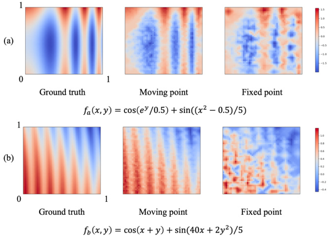
Figure 3. Comparison between the moving point and the fixed point representations through the fitting. Our proposed moving point representations can approximate given continuous functions with higher accuracy.
图 3: 移动点与固定点表示法在拟合过程中的对比。我们提出的移动点表示法能以更高精度逼近给定连续函数。
4.2. Sequential data classification
4.2. 序列数据分类
To demonstrate that SMPConv can handle long-term dependencies well, we evaluated our method on various sequential data tasks, such as sequential image and time-series classification. To do so, we followed FlexTCN [48] to construct a SMPConv architecture for causal 1D CNN whose kernel size is same as the input sequence length. We substituted their parameterized kernels with ours without additional modifications. To maintain a similar number of network parameters, SMPConv contains 30 weight points in each SMP. To alleviate the computation burdens caused by the convolution with large kernels, we have considered exploiting the computations through a fast Fourier transform. More network and experimental details are in Appendix A.1.
为验证SMPConv能有效处理长程依赖关系,我们在序列图像分类和时间序列分类等任务上评估了该方法。参照FlexTCN [48]的架构设计,我们构建了因果一维卷积网络(causal 1D CNN)的SMPConv实现,其卷积核尺寸与输入序列长度相同。在保持网络参数量相近的前提下(每个SMP包含30个权重点),我们直接替换了原方案的参数化卷积核。针对大尺寸卷积核带来的计算负担,我们探索了基于快速傅里叶变换的加速方案。完整网络结构与实验细节见附录A.1。
Sequential image. We tested our SMPConv on the 1D version of images from the datasets, sequential MNIST (sMNIST), permuted MNIST(pMNIST) [32], and sequential CIFAR10 (sCIFAR10) [4]. These datasets have long input sequence lengths, for example, 784 for sMNIST and pMNIST, and 1024 for sCIFAR10. Note that it is hard to model these datasets without proper kernel representations.
序列图像。我们在数据集的一维版本上测试了SMPConv,包括顺序MNIST (sMNIST)、置换MNIST (pMNIST) [32] 和顺序CIFAR10 (sCIFAR10) [4]。这些数据集具有较长的输入序列长度,例如sMNIST和pMNIST为784,sCIFAR10为1024。需要注意的是,如果没有合适的核表示,对这些数据集进行建模将非常困难。
Table 2. Sequential image classification results.
表 2: 序列图像分类结果
| 模型 | 参数量 | sMNIST | pMNIST | sCIFAR10 |
|---|---|---|---|---|
| DilRNN [4] | 44k | 98.0 87.2 | 96.1 | |
| LSTM [2] | 70k | 85.7 | ||
| GRU [2] | 70k | 96.2 | 87.3 | |
| TCN [2] | 70k | 99.0 | 97.2 | |
| r-LSTM [61] | 500k | 98.4 | 95.2 | 72.2 |
| IndRNN [33] | 83k | 99.0 | 96.0 | |
| TrellisNet [3] | 8M | 99.20 99.28 | 98.13 | 73.42 |
| URLSTM [21] | - | 96.96 | 71.00 | |
| HiPPO [19] | 0.5M | 98.30 | ||
| coRNN [51] | 134k | 99.4 | 97.3 | |
| CKCNN [49] | 98k | 99.31 | 98.00 | 62.25 |
| LSSL [22] | 99.53 | 98.76 | 84.65 | |
| S4 [20] | 99.63 | 98.70 | 91.13 | |
| FlexTCN [48] Ours | 375k 373k | 99.62 99.75 | 98.63 | 80.82 84.86 |
As shown in Tab. 2, the proposed model has achieved stateof-the-art results on both sMNIST and pMNIST. For sCIFAR10 dataset, our model has outperformed all the comparative models except S4 [20]. Compared with the FlexTCN, which has a similar network base, our model improved the accuracy by $4%$ . These results show that our proposed model is suitable and effective for sequential images.
如表 2 所示,所提出的模型在 sMNIST 和 pMNIST 上均取得了最先进的结果。对于 sCIFAR10 数据集,我们的模型表现优于除 S4 [20] 之外的所有对比模型。与网络结构相似的 FlexTCN 相比,我们的模型将准确率提高了 $4%$。这些结果表明,我们提出的模型适用于序列图像且效果显著。
Time-series. We evaluated our model on time-series sequence datasets, character trajectories (CT) [1], and speech commands (SC) [64]. The results have been displayed in Tab. 3. In the relatively shorter MFCC features data, SMPConv achieved test accuracy similar to FlexTCN. To validate that our proposed model can model extremely long sequences, we conducted experiments on the SC-raw dataset, which has a sequence length of 16000. Similar to the sequence image classification result, our model outperformed FlexTCN with a large margin of $+3%$ .
时间序列。我们在时间序列数据集、字符轨迹(CT) [1]和语音命令(SC) [64]上评估了模型性能,结果如表3所示。在较短的MFCC特征数据上,SMPConv取得了与FlexTCN相近的测试准确率。为验证模型对超长序列的建模能力,我们在序列长度达16000的SC-raw数据集上进行了实验。与序列图像分类结果类似,我们的模型以$+3%$的显著优势超越FlexTCN。
Compared to other models, our SMPConv has achieved considerably better performance for both sequential image and time-series classification. It ensures that our kernel represent ation is capable of handling long-term dependencies even in the case of a limited number of parameters.
与其他模型相比,我们的SMPConv在序列图像和时间序列分类任务上都实现了显著更优的性能。该设计确保即使在参数数量有限的情况下,我们的核表示仍能有效处理长程依赖关系。
4.3. Image classification
4.3. 图像分类
Image classification with the continuous kernel. We validated our SMPConv on a 2D image dataset, CIFAR10 [31], which is dominated by discrete convolutions, to show that the continuous kernel can capture spatial information as well. Similar to the experiments on sequential data, we followed the network design choice of FlexNet [48], where the kernel size is $33\times33$ . More details are in Appendix A.1.
使用连续核进行图像分类。我们在以离散卷积为主的2D图像数据集CIFAR10 [31]上验证了SMPConv,证明连续核同样能捕捉空间信息。与序列数据实验类似,我们遵循FlexNet [48]的网络设计选择,其中核尺寸为$33\times33$。更多细节见附录A.1。
As shown in Tab. 4, our continuous kernel representation model slightly outperforms ResNet, a discrete $3\times3$ convolution model, with a less number of parameters. It implies that our model is competitive and promising. Our model also showed better performance than MLP-based counterparts, CKCNN-16 and FlexNet-16, even when the parameters of ours were around $30%$ lesser. In addition, we have already identified the efficiency of our model in Tab. 1. These results suggest that our method is more suitable for kernel generation than MLP-based implicit formulations.
如表 4 所示,我们的连续核表示模型在参数更少的情况下略微优于 ResNet (一种离散的 $3\times3$ 卷积模型)。这表明我们的模型具有竞争力且前景良好。即使我们的模型参数比基于 MLP 的 CKCNN-16 和 FlexNet-16 少约 $30%$,其性能仍优于它们。此外,我们已在表 1 中证实了该模型的高效性。这些结果表明,相比基于 MLP 的隐式公式,我们的方法更适合核生成任务。
Table 3. Time-series classification results.
表 3: 时间序列分类结果
| Model | Params. | CT | SC | SC-raw |
|---|---|---|---|---|
| GRU-ODE [12] GRU-△t [29] GRU-D [5] ODE-RNN [50] NCDE [29] CKCNN [49] | 89k 89k 89k 89k 89k 100k | 96.2 97.8 95.9 97.1 98.8 99.53 | 44.8 20.0 23.9 93.2 88.5 95.27 | ~10.0 > 10.0 > 10.0 > 10.0 ~ 10.0 71.66 |
| LSSL [22] S4 [20] FlexTCN [48] Ours | - 373k 371k | 99.53 99.53 | 93.58 93.96 97.67 97.71 | 98.32 91.73 94.95 |
Table 4. 2D image classification on CIFAR10.
表 4: CIFAR10 上的二维图像分类
| 模型 | 参数量 | 准确率 |
|---|---|---|
| ResNet-44 [25] | 660k | 92.9 |
| CKCNN-16 [48] | 630k | 72.1 |
| FlexNet-16 [48] | 670k | 92.2 |
| Ours | 490k | 93.0 |
Large scale image classification. Finally, we tested our SMPConv on a large-scale ImageNet dataset [13], which contains more than one million training images and 50,000 validation images. For such a large dataset, the convolution kernels should be carefully trained to model complex data relationships accurately. Through such an experiment, therefore, we can validate that our SMP can represent a descriptive convolution kernel.
大规模图像分类。最后,我们在包含超过一百万张训练图像和五万张验证图像的大规模ImageNet数据集[13]上测试了SMPConv。对于如此庞大的数据集,需要精心训练卷积核以准确建模复杂的数据关系。因此,通过该实验我们能够验证SMP可以表征具有强描述能力的卷积核。
Firstly, we constructed large-scale variants of SMPConv architecture based on RepLKNet [14]. We replaced its discrete depth-wise separable convolution kernel with our SMP. In general, the larger the data and network, the larger the number of filters. To prevent excessive point position parameters depending on the number of filters, we shared the position of points over filters in large-scale settings. We empirically found that this position sharing has little effect on classification performance.
首先,我们基于RepLKNet [14]构建了SMPConv架构的大规模变体。我们用SMP替换了其离散的深度可分离卷积核。一般来说,数据和网络规模越大,滤波器数量就越多。为防止点位置参数因滤波器数量过多而激增,我们在大规模设置中跨滤波器共享了点位置。实证发现这种位置共享对分类性能影响甚微。
We proposed two variants of our model, SMPConv-T and SMPConv-B. Thanks to our efficient large kernel, we adjusted the number of channels and blocks so that our variants have a similar number of parameters to the previous models. The number of blocks and channels for each stage is [2, 2, 8, 2] and [96, 192, 384, 768] for SMPConv-T and [2, 2, 20, 2] and [128, 256, 512, 1024] for SMPConv
我们提出了模型的两种变体:SMPConv-T和SMPConv-B。得益于高效的大核设计,我们调整了通道数和块数,使变体参数规模与先前模型相近。SMPConv-T的各阶段块数和通道数分别为[2, 2, 8, 2]和[96, 192, 384, 768],SMPConv-B则为[2, 2, 20, 2]和[128, 256, 512, 1024]。
Table 5. 2D image classification on ImageNet-1K.
表 5: ImageNet-1K 二维图像分类
| 模型 | 参数量 | 计算量 (FLOPs) | Top-1准确率 |
|---|---|---|---|
| ResNet-50[25] | 26M | 4.1G | 76.5 |
| ResNext-50-32x4d [68] | 25M | 4.3G | 77.6 |
| 79.4 | |||
| ResMLP-S24[59] | 30M | 6.0G | 79.8 |
| DeiT-S [60] | 22M | 4.6G | 81.3 |
| Swin-T [37] | 28M | 4.5G | 81.3 |
| TNT-S [23] | 24M | 5.2G | |
| ConvNeXt-T[38] | 29M | 4.5G | 82.1 |
| SLaK-T [35] | 30M | 5.0G | 82.5 |
| SMPConv-T(ours) | 27M | 5.7G | 82.5 |
| DeiT-Base/16[60] | 87M | 17.6G | 81.8 |
| Swin-B [37] | 88M | 15.4G | 83.5 |
| ConvNeXt-B [38] | 89M | 15.4G | 83.8 |
| SLaK-B [35] | 95M | 17.1G | 84.0 |
| RepLKNet-31B [14] | 79M | ||
| SMPConv-B(ours) | 80M | 15.3G | 83.5 |
| 16.6G | 83.8 |
Table 6. Ablation study on CIFAR10. A checkmark means that the component is a learnable. In case of SMPConv, for instance, both radius and coordinate are learnable parameters.
| Models | radius | coordinate | Accuracy |
| A | 90.92 | ||
| B | 人 | 91.35 | |
| C | 人 | 92.47 | |
| SMPConv | √ | 人 | 93.00 |
表 6: CIFAR10消融实验。勾选标记表示该组件为可学习参数。例如在SMPConv中,半径(radius)和坐标(coordinate)均为可学习参数。
| 模型 | radius | coordinate | 准确率 |
|---|---|---|---|
| A | 90.92 | ||
| B | ✓ | 91.35 | |
| C | ✓ | 92.47 | |
| SMPConv | ✓ | ✓ | 93.00 |
Table 7. Classification results on CIFAR10 with different standard deviation $\sigma$ of point location sampling distribution.
表 7: 不同点位置采样分布标准差 $\sigma$ 在 CIFAR10 上的分类结果
| b | 0.05 | 0.2 | 0.3 | 0.5 |
|---|---|---|---|---|
| 准确率 | 93.00 | 92.24 | 91.84 | 91.51 |
Table 8. Classification results on CIFAR10 with different initial radius $r$ .
| r | 0.12 | 0.18 | 0.24 | 0.3 |
| Accuracy | 93.00 | 92.36 | 92.06 | 91.76 |
表 8: 不同初始半径 $r$ 在 CIFAR10 上的分类结果
| r | 0.12 | 0.18 | 0.24 | 0.3 |
|---|---|---|---|---|
| 准确率 | 93.00 | 92.36 | 92.06 | 91.76 |
B, respectively. In RepLKNet-31B, the number of blocks and channels for each stage is [2, 2, 18, 2] and [128, 256, 512, 1024]. More experimental details are provided in Appendix A.2.
在RepLKNet-31B中,各阶段的块数和通道数分别为[2, 2, 18, 2]和[128, 256, 512, 1024]。更多实验细节见附录A.2。
As reported in Tab. 5, our models obtained competitive performance with fewer parameters than existing models. These results show that our kernel representation is promising for large-scale domains as well. Overall, our kernel represent ation is highly effective and descriptive.
如表 5 所示,我们的模型在参数更少的情况下取得了与现有模型相当的性能。这些结果表明,我们的核表示在大规模领域也很有前景。总体而言,我们的核表示非常高效且具有描述性。
4.4. Ablation
4.4. 消融实验
We performed various ablation studies with additional experiments on CIFAR10 image classification. First, we investigated the validity of learnable radius and coordinate. In Tab. 6, it showed that performance degradation occurs when either one or both components are set to non-learnable parameters. Remarkably, Model C, which set coordinate to trainable parameters, outperformed Model A by a considerable margin. Furthermore, Model B also had a slight performance gain. It suggests that even randomly distributed fixed weight points can increase their interpolation ability with trainable radius. These results indicate that training both coordinate and radius is valid.
我们在CIFAR10图像分类任务上进行了多项消融实验。首先验证了可学习半径与坐标的有效性。表6显示:当任一组件或两者被设为不可学习参数时均会出现性能下降。值得注意的是,将坐标设为可训练参数的Model C显著优于Model A,而Model B也获得了小幅性能提升。这表明即使随机分布的固定权重点,也能通过可训练半径提升插值能力。这些结果证实同时训练坐标和半径是有效的。
Table 9. Classification results on CIFAR10 with different number of moving points $N_{p}$ .
表 9: 不同移动点数 $N_{p}$ 在 CIFAR10 上的分类结果
| Np | 4 | 8 | 16 | 32 | 64 |
|---|---|---|---|---|---|
| 参数量 | 250k | 330k | 490k | 809k | 1447k |
| 准确率 | 92.56 | 92.28 | 93.00 | 92.84 | 92.21 |
Next, we identified the effect of the initial position of the points by varying the $\sigma$ , a standard deviation of point location sampling distribution. In Tab. 7, we observed that a small $\sigma$ value, indicating initial positions of the points are gathered in the center of the kernel, leads to higher accuracy. This is because it is difficult to train large kernels from the beginning of training. Thus, large kernels can be effectively trained by starting with small kernels and expanding the receptive fields through moving points.
接下来,我们通过改变点位置采样分布的标准差 $\sigma$ 来识别点初始位置的影响。在表 7 中,我们观察到较小的 $\sigma$ 值(表示点的初始位置聚集在卷积核中心)会带来更高的准确率。这是因为从一开始就训练大卷积核较为困难。因此,通过从小卷积核开始训练,并通过移动点逐步扩大感受野,可以更有效地训练大卷积核。
We also found that larger initial radius degrades the model performance as shown in Tab. 8. The large radius results in a large initial kernel size, which makes initial training difficult. Furthermore, it is also challenging to train a large area of the kernel dependent on a single weight point which is not optimized in the early stages of training. Both Tab. 7 and Tab. 8 empirically show that our initialization methods for SMP are effective.
我们还发现,如表8所示,较大的初始半径会降低模型性能。大半径会导致初始卷积核尺寸过大,使得初期训练变得困难。此外,依赖单个未优化权重点来训练大范围卷积核区域也极具挑战性。表7和表8均通过实验证明,我们提出的SMP初始化方法是有效的。
As depicted in Tab. 9, we figured out that simply increasing the number of weight points $N_{p}$ does not helpful for performance. It implies that a small number of points are enough to represent a proper convolution filter. Since the performance is influenced by the number of points, our method is also required tuning like common neural networks. However, the performance difference between CKCNN and FlexNet in Tab. 4 shows that MLP-based methods are severely influenced by architectural settings. That is, they have extensive search space, such as depth, width, and activation function, so they typically require more tuning than our method. Moreover, the impact of the number of points is not particularly significant in that even the worst $(N_{p}=64$ ) slightly outperforms the FlexNet $\yen123,456$ ).
如表 9 所示,我们发现单纯增加权重点数量 $N_{p}$ 对性能并无帮助。这表明少量点足以表征合适的卷积滤波器。由于性能受点数影响,我们的方法也需要像普通神经网络那样进行调参。但表 4 中 CKCNN 与 FlexNet 的性能差异表明,基于 MLP 的方法受架构设置影响严重——它们存在深度、宽度和激活函数等广阔的搜索空间,因此通常比我们的方法需要更多调参。此外,点数的影响并不特别显著,因为即使最差情况 $(N_{p}=64$ ) 也略微优于 FlexNet $\yen123,456$ )。
4.5. Visualization
4.5. 可视化
Finally, we analyze our SMP by visualizing filters trained on CIFAR10. In the first column of Fig. 4, we can observe the trained weight points’ position. In our method, point locations $p_{i}$ are mainly sampled near the center of the kernel for stable training. It shows that the points spread out for optimal kernel representation over the training process, as we argued, and thus the receptive fields are not limited to a small part. Also, we can figure out that there are square patterns caused by Eq. (2) in the kernels, where each square has its own area. This suggests that although the radius parameters are initialized with small values, the values are individually increased and optimized for each corresponding weight point during training.
最后,我们通过可视化在CIFAR10上训练得到的滤波器来分析SMP。在图4的第一列中,可以观察到训练后权重点的位置分布。在我们的方法中,点位置$p_{i}$主要采样于卷积核中心附近以确保训练稳定性。结果表明,正如我们所论证的,这些点在训练过程中逐渐扩散以形成最优核表示,因此感受野并不局限于小范围区域。此外,可以观察到由公式(2)在卷积核中产生的方形模式,每个方形区域具有独立的作用范围。这说明尽管半径参数初始值较小,但在训练过程中会针对每个权重点单独进行增大和优化。

Figure 4. Visualization of kernels. Each row shows the location of points and first 6 kernels of a filter. For ease of visualization, the kernels are first subjected to the absolute value operation and then normalized to a range of [0,1].
图 4: 核可视化。每行展示了一个滤波器的点位置及其前6个核。为便于观察,核先经过绝对值运算再归一化至[0,1]范围。

Figure 5. Normalized sum of the absolute value of trained filters. (a), (b), and (c) are top, middle, and bottom layers, respectively.
图 5: 训练滤波器绝对值归一化总和。(a)、(b)和(c)分别对应顶层、中层和底层。
Observing visualized convolution kernel in Fig. 4, kernels from the same filter share the receptive fields. It allows a single filter to focus on the shared area. Furthermore, as illustrated in Fig. 5, SMPConv has large adaptive receptive fields which are not conventional square or rectangular shapes. This is because it consists of optimized filters with their own small and large receptive fields. Thus, our method can handle not only global information but also local details.
观察图4中可视化的卷积核,同一滤波器中的核共享感受野。这使得单个滤波器能够专注于共享区域。此外,如图5所示,SMPConv具有较大的自适应感受野,这些感受野并非传统的方形或矩形。这是因为其由优化后的滤波器组成,这些滤波器各自拥有小型和大型感受野。因此,我们的方法不仅能处理全局信息,还能捕捉局部细节。
5. Conclusion and discussion
5. 结论与讨论
In this paper, we present a method to build a continuous convolution. We propose using point representations, where each point has the weight parameters, coordinates, and radius to learn. By connecting the points, we can implement a continuous function, which can be utilized to construct convolutional kernels. We have provided extensive experimental results, showing that drop-in replacement in the existing training pipeline without bells and whistles improved the performance by a safe margin. We also show that a continuous convolution can be effectively utilized in a large-scale experiment. We expect more research and development in this direction.
本文提出了一种构建连续卷积的方法。我们建议采用点表示法,其中每个点包含待学习的权重参数、坐标和半径。通过连接这些点,我们可以实现一个连续函数,进而用于构建卷积核。我们提供了大量实验结果,表明在现有训练流程中直接替换该方法(无需额外修饰)即可稳定提升性能。同时,我们证明了连续卷积在大规模实验中能够有效应用。期待该方向涌现更多研究与发展。
Although promising, there are many rooms to be improved. Due to the limited computational budget, we could not conduct sufficient experiments in the large-scale experiment. The experimental results provided in this manuscript resulted from a few runs. As trial and error are essential in the machine learning development process, we plan to find optimal configurations and training techniques to enhance the performance of the proposed method.
尽管前景广阔,但仍有诸多改进空间。由于计算资源有限,我们无法在大规模实验中开展充分验证。本文提供的实验结果仅基于少量运行得出。鉴于试错法是机器学习开发过程中的关键环节,我们计划通过寻找最优配置和训练技术来提升所提方法的性能。
We also observed that the learned kernels often show sparse patterns depending on the tasks. It is well aligned with the success of dilated convolution or its variants, and our methods automatically learn proper sparsity during the training process on specific tasks. Adding prior knowledge through training and regular iz ation techniques would further improve performance, especially for tasks requiring longer-term dependency modeling.
我们还发现,学习到的核(kernel)通常会根据任务呈现稀疏模式。这一现象与扩张卷积(dilated convolution)及其变体的成功应用高度吻合,而我们的方法能在特定任务训练过程中自动学习适当的稀疏性。通过训练和正则化(regularization)技术融入先验知识,将进一步提升性能,尤其对于需要更长程依赖建模的任务。
Acknowledgments
致谢
We thank Usman Ali for valuable discussions. This research was supported by the Ministry of Science and ICT (MSIT) of Korea, under the National Research Foundation (NRF) grant (2022 R 1 F 1 A 1064184, 2022 R 1 A 4 A 3033571), Institute of Information and Communication Technology Planning Evaluation (IITP) grants for the AI Graduate School program (IITP-2019-0-00421), and the BK21 FOUR Project.
我们感谢Usman Ali富有价值的讨论。本研究由韩国科学技术信息通信部(MSIT)资助,项目包括韩国国家研究基金会(NRF)资助(2022 R1F1A1064184、2022 R1A4A3033571)、信息通信技术规划评估院(IITP)的人工智能研究生院项目资助(IITP-2019-0-00421),以及BK21 FOUR项目。
References
参考文献
SMPConv: Self-moving Point Representations for Continuous Convolution Appendix
SMPConv:连续卷积的自移动点表示附录
A. Experimental details
A. 实验细节
A.1. Sequential data and image classification
A.1. 序列数据与图像分类
In each convolution filter, SMPConv has 30 weight points for 1D and 16 weight points for 2D. For SMPConv1D, we sample the point locations from zero mean truncated gaussian distribution with $\sigma=0.1$ . Because of causal convolution, we sample in the range $(-1,0)$ rather than $(-1,1)$ . For SMPConv2D, we sample the point locations from 2D zero mean truncated gaussian with $\Sigma=$ $[[\sigma_{1},0],[0,\sigma_{2}]]$ , where $\sigma_{1}=\sigma_{2}=0.05$ . We initialize radius as $\begin{array}{r}{r\approx\frac{2}{k}d}\end{array}$ , where $k$ is kernel size and $d$ is dimension of input (i.e., $d=1$ for 1D, $d=2$ for 2D). In 2D, the kernel size means the width of the kernel. The size of the additional small kernel is 5 for 1D and $3\times3$ for 2D, respectively. Following FlexConv [48], we use batch normalization [28] after convolution and skip connection.
在每个卷积滤波器中,SMPConv为1D卷积设置30个权重点,为2D卷积设置16个权重点。对于SMPConv1D,我们从$\sigma=0.1$的零均值截断高斯分布中采样点位置。由于因果卷积的限制,采样范围设定为$(-1,0)$而非$(-1,1)$。对于SMPConv2D,点位置采样自二维零均值截断高斯分布,其协方差矩阵为$\Sigma=[[\sigma_{1},0],[0,\sigma_{2}]]$,其中$\sigma_{1}=\sigma_{2}=0.05$。半径初始化为$\begin{array}{r}{r\approx\frac{2}{k}d}\end{array}$,这里$k$表示核尺寸,$d$代表输入维度(即1D时$d=1$,2D时$d=2$)。在2D情况下,核尺寸指核的宽度。附加小核的尺寸在1D时为5,2D时为$3\times3$。参照FlexConv [48]的做法,我们在卷积后采用批归一化[28]并添加跳跃连接。
We train our networks using Adam [30] optimizer. We use a cosine annealing learning rate scheduling with warmup epochs. The learning rate for radius parameters is set to be $0.1\times$ smaller than the regular learning rate. During the training, the radius range is clipped from 0.0001 to 1.0. More details for each data are shown in Tab. 10. For sequential data experiments, we train our model with a single NVIDIA A100 GPU. We use a single RTX3090 GPU for CIFAR10 experiments.
我们使用Adam [30]优化器训练网络,采用带预热周期的余弦退火学习率调度策略。半径参数的学习率设置为常规学习率的$0.1\times$。训练过程中,半径范围被限制在0.0001到1.0之间。各数据集详细配置见 表10。序列数据实验使用单张NVIDIA A100 GPU进行训练,CIFAR10实验则使用单张RTX3090 GPU。
A.2. Image classification on ImageNet-1k
A.2. ImageNet-1k 图像分类
Our large-scale variants of SMPConv networks have the same architecture as RepLKNet [14] except for large kernel convolution, which is replaced by our SMP. Like [14], we set the kernel size of each stage to [31, 29, 27, 13] and use additional $5\times5$ convolution for re parameter iz ation trick. We use $\left\lfloor{\frac{k^{2}}{4}}\right\rfloor$ weight points for each SMP depth-wise version, which shares weight points over channels, where $k$ is the kernel size of corresponding each block. The point locations and radius are initialized in the same way as Appendix A.1 SMPConv2D with $\sigma_{1}=\sigma_{2}=0.2$ .
我们的大规模SMPConv变体网络与RepLKNet[14]架构相同,只是将大核卷积替换为我们的SMP模块。参照[14],我们将每个阶段的卷积核尺寸设置为[31, 29, 27, 13],并额外使用$5\times5$卷积进行重参数化处理。对于每个SMP深度可分离版本,我们采用$\left\lfloor{\frac{k^{2}}{4}}\right\rfloor$个权重点(其中$k$为对应模块的卷积核尺寸),这些权重点在通道间共享。权重点位置与半径的初始化方式与附录A.1中$\sigma_{1}=\sigma_{2}=0.2$的SMPConv2D保持一致。
Our models are trained for 300 epochs using AdamW [39] optimizer. We set the batch size of 2048. The initial learning rate is set to $4\times10^{-3}$ with cosine annealing scheduling and 10 warm-up epochs. We use Rand Augment [9] in Timm 65, Label Smoothing [55] coefficient of 0.1, Mixup [74] with $\alpha=0.8$ , Cutmix [73] with $\alpha=1.0$ , Rand Erasing [76] with probability of $25%$ , Stochastic Depth with drop path rate of $10%$ for SMPConv-T, and $50%$ for SMPConv-B, and model EMA(exponential moving average) with a decay factor of 0.9999. For fast depth-wise convolution computation, we use block-wise(inverse) implicit gemm algorithm implemented by [14]. We train both SMPConv-T and SMPConv-B with 4 NVIDIA A100 GPUs.
我们的模型使用AdamW [39]优化器训练300个周期,批次大小设为2048。初始学习率设置为$4\times10^{-3}$,采用余弦退火调度并包含10个预热周期。数据增强采用Timm库[65]中的Rand Augment9,标签平滑[55]系数设为0.1,Mixup[74]参数$\alpha=0.8$,Cutmix[73]参数$\alpha=1.0$,随机擦除[76]概率为$25%$。随机深度(Stochastic Depth)的路径丢弃率在SMPConv-T中设为$10%$,SMPConv-B中设为$50%$。模型采用指数移动平均(EMA)且衰减因子为0.9999。为实现快速深度卷积计算,我们采用[14]实现的块状(逆)隐式gemm算法。所有训练均在4块NVIDIA A100 GPU上完成,包括SMPConv-T和SMPConv-B模型。
B. Additional results
B. 补充结果
B.1. Larger kernels
B.1. 更大的卷积核
We set the kernel size of each stage to [31, 29, 27, 13] for large-scale variants of SMPConv networks following RepLKNet [14]. Although the current kernel sizes are larger than conventional convolution, we evaluate whether our model is trained without performance degradation even when using larger kernels.
我们按照RepLKNet [14]的方法,为SMPConv网络的大规模变体设置了各阶段的卷积核大小为[31, 29, 27, 13]。尽管当前的卷积核尺寸大于传统卷积,但我们评估了模型在使用更大卷积核时是否仍能无性能下降地完成训练。
To conduct this experiment, we design a new variant, SMPConv-mobile. For the mobile variant, the number of blocks and the number of channels for each stage is [2, 2, 2, 2] and [64, 128, 256, 320], respectively. Also, we use $\left\lfloor{\frac{k^{2}}{8}}\right\rfloor$ weight points for each SMP and reduce the expansion ratio of feed-forward networks from 4 to 2. We train this variant for 120 epochs and do not use Stochastic Depth. Other training settings are same as Appendix A.2. We set the kernel size of each stage to [31, 29, 27, 13] for SMPConvmobile31 and [51, 49, 47, 13] for SMPConv-mobile51.
为进行本实验,我们设计了一个新变体SMPConv-mobile。该移动版变体各阶段的块数和通道数分别为[2, 2, 2, 2]和[64, 128, 256, 320]。同时,我们为每个SMP使用$\left\lfloor{\frac{k^{2}}{8}}\right\rfloor$个权重点,并将前馈网络的扩展比从4降至2。该变体训练120个周期且不使用随机深度(Stochastic Depth),其他训练设置与附录A.2相同。我们将SMPConv-mobile31各阶段的卷积核尺寸设为[31, 29, 27, 13],SMPConv-mobile51则设为[51, 49, 47, 13]。
In ImageNet-1k [13] image classification, SMPConvmobile31 and SMPConv-mobile51 get $73.5%$ and $73.7%$ top-1 accuracy, respectively. Thus, using our SMP, convolution kernel sizes can be increased without performance degradation, even in large-scale data.
在ImageNet-1k [13]图像分类任务中,SMPConvmobile31和SMPConv-mobile51分别取得了73.5%和73.7%的top-1准确率。这表明即使在大规模数据场景下,采用我们的SMP方法也能在增大卷积核尺寸的同时保持性能不下降。
Table 10. Hyper-parameter details
表 10. 超参数详情
| SMNIST | pMNIST | SCIFAR10 | CT | SC | SC-raw | CIFAR10 | |
|---|---|---|---|---|---|---|---|
| lr | 0.0001 | 0.0001 | 0.0002 | 0.0001 | 0.002 | 0.001 | 0.005 |
| epoch | 200 | 200 | 200 | 300 | 300 | 160 | 210 |
| warm-up | 5 | 5 | 5 | 5 | 5 | 10 | 10 |
| dropout | 0 | 0 | 0 | 0 | 0.2 | 0.1 | 0.1 |
| #ofbatch | 64 | 64 | 64 | 64 | 32 | 32 | 64 |
| weight decay | 1e-5 | 1e-5 | 1e-5 | 1e-5 | 1e-5 | 1e-5 | 1e-5 |
| kernelsize | 784 | 784 | 1024 | 182 | 161 | 16000 | 33×33 |