PREDICTIVE CODING APPROXIMATES BACKPROP ALONG ARBITRARY COMPUTATION GRAPHS
预测编码沿任意计算图近似反向传播
Beren Millidge
Beren Millidge
Alexander Tschantz
Alexander Tschantz
School of Informatics University of Edinburgh beren@millidge.name
爱丁堡大学信息学院 beren@millidge.name
Sackler Centre for Consciousness Science School of Engineering and Informatics University of Sussex tschantz.alec@gmail.com
萨克勒意识科学中心
萨塞克斯大学工程与信息学院
tschantz.alec@gmail.com
Christopher L Buckley Evolutionary and Adaptive Systems Research Group School of Engineering and Informatics University of Sussex C.L.Buckley@sussex.ac.uk
Christopher L Buckley
进化与自适应系统研究组
工程与信息学院
萨塞克斯大学
C.L.Buckley@sussex.ac.uk
October 7, 2020
2020年10月7日
ABSTRACT
摘要
Back propagation of error (backprop) is a powerful algorithm for training machine learning architectures through end-to-end differentiation. Recently it has been shown that backprop in multilayerperce ptr on s (MLPs) can be approximated using predictive coding, a biologically-plausible process theory of cortical computation which relies solely on local and Hebbian updates. The power of backprop, however, lies not in its instantiation in MLPs, but rather in the concept of automatic differentiation which allows for the optimisation of any differentiable program expressed as a computation graph. Here, we demonstrate that predictive coding converges asymptotically (and in practice rapidly) to exact backprop gradients on arbitrary computation graphs using only local learning rules. We apply this result to develop a straightforward strategy to translate core machine learning architectures into their predictive coding equivalents. We construct predictive coding CNNs, RNNs, and the more complex LSTMs, which include a non-layer-like branching internal graph structure and multiplicative interactions. Our models perform equivalently to backprop on challenging machine learning benchmarks, while utilising only local and (mostly) Hebbian plasticity. Our method raises the potential that standard machine learning algorithms could in principle be directly implemented in neural circuitry, and may also contribute to the development of completely distributed neuro m orphic architectures.
误差反向传播(backprop)是一种通过端到端微分训练机器学习架构的强大算法。近期研究表明,多层感知机(MLPs)中的反向传播可通过预测编码(predictive coding)进行近似——这是一种仅依赖局部更新与赫布学习的生物可解释性皮层计算过程理论。然而反向传播的核心优势并不在于其在MLPs中的实现,而在于自动微分(automatic differentiation)这一概念,它能优化任何表示为计算图的可微分程序。本文证明:预测编码仅使用局部学习规则即可渐近收敛(实践中能快速收敛)至任意计算图上的精确反向传播梯度。基于此发现,我们提出一种将核心机器学习架构转换为预测编码等效模型的直接策略,构建了预测编码版CNN、RNN以及具有非层级分支图结构和乘法交互的复杂LSTM模型。在挑战性机器学习基准测试中,我们的模型表现与反向传播相当,且仅使用局部(及主要基于赫布)的可塑性机制。该方法揭示了标准机器学习算法在神经环路中直接实现的潜在可能性,也可能推动完全分布式神经形态架构的发展。
1 Introduction
1 引言
Deep learning has seen stunning successes in the last decade in computer vision (Krizhevsky, Sutskever, & Hinton, 2012; Szegedy et al., 2015), natural language processing and translation (Kaplan et al., 2020; Radford et al., 2019; Vaswani et al., 2017), and computer game playing (Mnih et al., 2015; Schr it t wiese r et al., 2019; Silver et al., 2017; Vinyals et al., 2019). While there is a great variety of architectures and models, they are all trained by gradient descent using gradients computed by automatic differentiation (AD). The key insight of AD is that it suffices to define a forward model which maps inputs to predictions according to some parameters. Then, using the chain rule of calculus, it is possible, as long as every operation of the forward model is differentiable, to differentiate back through the computation graph of the model so as to compute the sensitivity of every parameter in the model to the error at the output, and thus adjust every single parameter to best minimize the total loss. Early models were typically simple artificial neural networks where the computation graph is simply a composition of matrix multiplications and element wise nonlinear i ties, and for which the implementation of automatic different ation has become known as ‘back propagation’ (or ’backprop’). However, automatic differentiation allows for substantially more complicated graphs to be differentiated through, up to, and including, arbitrary programs (Baydin, Pearl mutter, Radul, & Siskind, 2017; Griewank et al., 1989; Innes et al., 2019; Linnainmaa, 1970; Paszke et al., 2017; Revels, Lubin, & Papamarkou, 2016; Rumelhart & Zipser, 1985; Werbos, 1982). In recent years this has enabled the differentiation through differential equation solvers (T. Q. Chen, Rubanova, Bettencourt, & Duvenaud, 2018; Rackauckas et al., 2019; Tzen & Raginsky, 2019), physics engines (Degrave, Hermans, Dambre, & Wyffels, 2019; Heiden, Millard, & Sukhatme, 2019), raytracers (Pal, 2019), and planning algorithms (Amos & Yarats, 2019; Okada, Rigazio, & Aoshima, 2017). These advances allow the straightforward training of models which intrinsically embody complex processes and which can encode significantly more prior knowledge and structure about a given problem domain than previously possible.
深度学习在过去十年中取得了惊人的成功,涵盖计算机视觉 (Krizhevsky, Sutskever, & Hinton, 2012; Szegedy et al., 2015)、自然语言处理与翻译 (Kaplan et al., 2020; Radford et al., 2019; Vaswani et al., 2017) 以及计算机游戏博弈 (Mnih et al., 2015; Schrittwieser et al., 2019; Silver et al., 2017; Vinyals et al., 2019)。尽管架构和模型种类繁多,它们都通过自动微分 (automatic differentiation, AD) 计算梯度的梯度下降法进行训练。自动微分的核心思想是:只需定义一个根据参数将输入映射为预测结果的前向模型,只要该模型的每个操作可微,就能利用微积分链式法则反向微分整个模型的计算图,从而计算模型中每个参数对输出误差的敏感度,进而调整所有参数以最小化总体损失。早期模型通常是简单的人工神经网络,其计算图仅由矩阵乘法和逐元素非线性变换构成,这类自动微分的实现被称为"反向传播"(backpropagation 或 backprop)。但自动微分能处理更复杂的计算图,甚至包括任意程序 (Baydin, Pearlmutter, Radul, & Siskind, 2017; Griewank et al., 1989; Innes et al., 2019; Linnainmaa, 1970; Paszke et al., 2017; Revels, Lubin, & Papamarkou, 2016; Rumelhart & Zipser, 1985; Werbos, 1982)。近年来,该技术已实现对微分方程求解器 (T. Q. Chen, Rubanova, Bettencourt, & Duvenaud, 2018; Rackauckas et al., 2019; Tzen & Raginsky, 2019)、物理引擎 (Degrave, Hermans, Dambre, & Wyffels, 2019; Heiden, Millard, & Sukhatme, 2019)、光线追踪器 (Pal, 2019) 和规划算法 (Amos & Yarats, 2019; Okada, Rigazio, & Aoshima, 2017) 的微分。这些突破使得模型能直接内化复杂过程,并编码比以往更丰富的领域先验知识与结构。
Modern deep learning has also been closely intertwined with neuroscience (Hassabis, Kumaran, Summer field, & Botvinick, 2017; Hawkins & Blakeslee, 2007; Richards et al., 2019). The back propagation algorithm itself arose as a technique for training multi-layer perce ptr on s – simple hierarchical models of neurons inspired by the brain (Werbos, 1982). Despite this origin, and its empirical successes, a consensus has emerged that the brain cannot directly implement backprop, since to do so would require biologically implausible connection rules (Crick, 1989). There are two principal problems. Firstly, backprop in the brain appears to require non-local information (since the activity of any specific neuron affects all subsequent neurons down to the final output neuron). It is difficult to see how this information could be transmitted ’backwards’ throughout the brain with the required fidelity without precise connectivity constraints. The second problem – the ‘weight transport problem’ is that backprop through MLP style networks requires identical forward and backwards weights. In recent years, however, a succession of models have been introduced which claim to implement backprop in MLP-style models using only biologically plausible connectivity schemes, and Hebbian learning rules (Bengio & Fischer, 2015; Bengio, Mesnard, Fischer, Zhang, & Wu, 2017; Guerguiev, Lillicrap, & Richards, 2017; Liao, Leibo, & Poggio, 2016; Ororbia, Mali, Giles, & Kifer, 2020; Sacramento, Costa, Bengio, & Senn, 2018; Whittington & Bogacz, 2019). Of particular significance is Whittington and Bogacz (2017) who show that predictive coding networks – a type of biologically plausible network which learn through a hierarchical process of prediction error minimization – are mathematically equivalent to backprop in MLP models. In this paper we extend this work, showing that predictive coding can not only approximate backprop in MLPs, but can approximate automatic differentiation along arbitrary computation graphs. This means that in theory there exist biologically plausible algorithms for differentiating through arbitrary programs, utilizing only local connectivity. Moreover, in a class of models which we call parameter-linear, which includes many current machine learning models, the required update rules are Hebbian, raising the possibility that a wide range of current machine learning architectures may be faithfully implemented in the brain, or in neuro m orphic hardware.
现代深度学习也与神经科学紧密交织(Hassabis, Kumaran, Summerfield, & Botvinick, 2017; Hawkins & Blakeslee, 2007; Richards et al., 2019)。反向传播算法本身是作为训练多层感知器(perceptron)的技术而出现的——这种简单的神经元层级模型受到大脑启发(Werbos, 1982)。尽管有这一渊源且取得了实证成功,学界已形成共识认为大脑无法直接实现反向传播,因为这需要生物学上不合理的连接规则(Crick, 1989)。主要存在两个问题:首先,大脑中的反向传播似乎需要非局部信息(因为任何特定神经元的活动都会影响后续所有神经元直至最终输出神经元)。很难想象在没有精确连接约束的情况下,这些信息如何以所需保真度在大脑中"反向"传递。第二个问题——"权重传输问题"在于,通过MLP风格网络的反向传播需要完全相同的前向和反向权重。然而近年来,一系列模型被提出,声称仅使用生物学合理的连接方案和Hebbian学习规则就能在MLP风格模型中实现反向传播(Bengio & Fischer, 2015; Bengio, Mesnard, Fischer, Zhang, & Wu, 2017; Guerguiev, Lillicrap, & Richards, 2017; Liao, Leibo, & Poggio, 2016; Ororbia, Mali, Giles, & Kifer, 2020; Sacramento, Costa, Bengio, & Senn, 2018; Whittington & Bogacz, 2019)。特别重要的是Whittington和Bogacz(2017)的研究,他们证明预测编码网络——一种通过预测误差最小化的层级过程进行学习的生物学合理网络——在数学上等价于MLP模型中的反向传播。本文扩展了这一工作,表明预测编码不仅能近似MLP中的反向传播,还能近似任意计算图上的自动微分。这意味着理论上存在仅使用局部连接的生物学合理算法,可用于对任意程序进行微分。此外,在我们称为参数线性的一类模型(包含许多当前机器学习模型)中,所需的更新规则是Hebbian式的,这提高了当前多种机器学习架构在大脑或神经形态硬件中忠实实现的可能性。
In this paper we provide two main contributions. (i) We show that predictive coding converges to automatic different i ation across arbitrary computation graphs. (ii) We showcase this result by implementing three core machine learning architectures (CNNs, RNNs, and LSTMs) in a predictive coding framework which utilises only local learning rules and mostly Hebbian plasticity.
本文提供了两项主要贡献:(i) 我们证明了预测编码(predictive coding)能在任意计算图中收敛到自动微分(automatic differentiation);(ii) 通过在预测编码框架中仅使用局部学习规则和以赫布可塑性(Hebbian plasticity)为主的机制,我们实现了三种核心机器学习架构(CNN、RNN和LSTM)的实例验证。
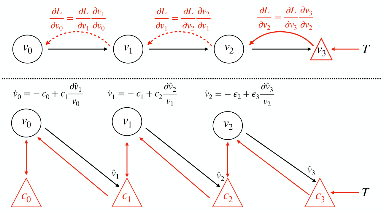
Figure 1: Top: Back propagation on a chain. Backprop proceeds backwawrds sequentially and explicitly computes the gradient at each step on the chain. Bottom: Predictive coding on a chain. Predictions, and prediction errors are updated in parallel using only local information.
图 1: 上: 链式反向传播。反向传播按顺序向后执行,并显式计算链上每一步的梯度。下: 链式预测编码。仅使用局部信息并行更新预测和预测误差。
2 Predictive Coding on Arbitrary Computation Graphs
2 任意计算图上的预测编码 (Predictive Coding)
Predictive coding is an influential theory of cortical function in theoretical and computational neuroscience. Central to the theory is the idea that the core function of the brain is to minimize prediction errors between what is expected to happen and what actually happens. Predictive coding views the brain as composed of multiple hierarchical layers which predict the activities of the layers below. Un predicted activity is registered as prediction error which is then transmitted upwards for a higher layer to process. Over time, synaptic connections are adjusted so that the system improves at minimizing prediction error. Predictive coding possesses a wealth of empirical support (Bogacz, 2017; Friston, 2003, 2005; Whittington & Bogacz, 2019) and offers a single mechanism that accounts for diverse perceptual phenomena such as repetition-suppression (Auks z tu lew i cz & Friston, 2016), end-stopping (Rao & Ballard, 1999), bistable perception (Hohwy, Roepstorff, & Friston, 2008; Weil n hammer, Stuke, Hesselmann, Sterzer, & Schmack, 2017) and illusory motions (Lotter, Kreiman, & Cox, 2016; Watanabe, Kitaoka, Sakamoto, Yasugi, & Tanaka, 2018), and even attention al modulation of neural activity (Feldman & Friston, 2010; Kanai, Komura, Shipp, & Friston, 2015). Moreover, the central role of top-down predictions is consistent with the ubiquity, and importance of, top-down diffuse connections between cortical areas. Predictive coding is consistent with many known aspects of neuro physiology, and has been translated into biologically plausible process theories which define candidate cortical micro circuits which can implement the algorithm. (Bastos et al., 2012; Kanai et al., 2015; Shipp, 2016; Spratling, 2008).
预测编码是理论和计算神经科学中极具影响力的皮层功能理论。该理论的核心观点是:大脑的基本功能在于最小化预期与实际发生情况之间的预测误差。预测编码将大脑视为由多个层级结构组成的系统,上层对下层活动进行预测,未预期的活动则被记录为预测误差并向上传递以供更高层级处理。随着时间的推移,突触连接会不断调整以使系统更好地最小化预测误差。预测编码理论拥有大量实证支持 (Bogacz, 2017; Friston, 2003, 2005; Whittington & Bogacz, 2019),其单一机制可解释多种感知现象,包括重复抑制 (Auks z tu lew i cz & Friston, 2016)、末端抑制 (Rao & Ballard, 1999)、双稳态知觉 (Hohwy, Roepstorff, & Friston, 2008; Weilnhammer, Stuke, Hesselmann, Sterzer, & Schmack, 2017) 和运动错觉 (Lotter, Kreiman, & Cox, 2016; Watanabe, Kitaoka, Sakamoto, Yasugi, & Tanaka, 2018),甚至神经活动的注意调节 (Feldman & Friston, 2010; Kanai, Komura, Shipp, & Friston, 2015)。此外,自上而下预测的核心作用与皮层区域间普遍存在的重要弥散性连接相吻合。该理论与神经生理学的诸多已知特征一致,并已转化为具有生物学合理性的加工理论,定义了可实现该算法的候选皮层微环路 (Bastos et al., 2012; Kanai et al., 2015; Shipp, 2016; Spratling, 2008)。
In previous work, predictive coding has always been conceptual is ed as operating on hierarchies of layers (Bogacz, 2017; Whittington & Bogacz, 2017). Here we present a generalized form of predictive coding applied to arbitrary computation graphs. A computation graph $\mathcal{G}={\mathbb{E},\mathbb{V}}$ is a directed acyclic graph (DAG) which can represent the computational flow of essentially any program or computable function as a composition of elementary functions. Each edge $e_{i}\in\mathbb{E}$ of the graph corresponds to an intermediate step – the application of an elementary function – while each vertex $v_{i}\in\mathbb{V}$ is an intermediate variable computed by applying the functions of the edges to the values of their originating vertices. In this paper, $v_{i}$ denotes the vector of activation s within a layer and we denote the set of all vertices as ${v_{i}}$ . Effectively, computation flows ’forward’ from parent nodes to all their children through the edge functions until the leaf nodes give the final output of the program as a whole (see Figure 1 and 2 for an example). Given a target $T$ and a loss function $L=g(T,v_{o u t})$ , the graph’s output can be evaluated and, and if every edge function is differentiable, automatic differentiation can be performed on the computation graph.
在以往的研究中,预测编码(predictive coding)一直被概念化为在层级结构上运作(Bogacz, 2017; Whittington & Bogacz, 2017)。本文提出了一种适用于任意计算图的广义预测编码形式。计算图$\mathcal{G}={\mathbb{E},\mathbb{V}}$是一个有向无环图(DAG),可以通过基本函数的组合来表示任何程序或可计算函数的计算流程。图中的每条边$e_{i}\in\mathbb{E}$对应一个中间步骤——即基本函数的应用,而每个顶点$v_{i}\in\mathbb{V}$则是通过对其起始顶点的值应用边函数计算得到的中间变量。本文中,$v_{i}$表示层内的激活向量,所有顶点的集合记为${v_{i}}$。实际上,计算沿着边函数从父节点"向前"流向所有子节点,直到叶节点给出程序的最终输出(示例见图1和图2)。给定目标$T$和损失函数$L=g(T,v_{o u t})$,可以评估图的输出,并且如果每个边函数都是可微的,就可以在计算图上执行自动微分。
Predictive coding can be derived elegantly as a variation al inference algorithm under a hierarchical Gaussian generative model (Buckley, Kim, McGregor, & Seth, 2017; Friston, 2005). We extend this approach to arbitrary computation graphs in a supervised setting by defining the inference problem to be solved as that of inferring the vertex value $v_{i}$ of each node in the graph given fixed start nodes $v_{0}$ (the data), and end nodes $v_{N}$ (the targets). We define a generative model which para met rises the value of each vertex given the feed forward prediction of its parents, $\begin{array}{r}{p({v_{i}})=\prod_{i}^{N}p(v_{i}|\mathcal{P}(v_{i}))}\end{array}$ , and a factorised, variation al posterior $\begin{array}{r}{Q({v_{i}})=\prod_{i}^{N}Q(v_{i})}\end{array}$ , where $\mathcal{P}(x)$ denotes the set of parents and ${\mathcal{C}}(x)$ denotes the set of children of a given node $\mathbf{X}$ . From this, we can define a suitable objective functional, the variation al free-energy $\mathcal{F}$ (VFE), which acts as an upper bound on the divergence between the true and variation al posteriors.
预测编码可以优雅地推导为层次高斯生成模型下的变分推断算法 (Buckley, Kim, McGregor, & Seth, 2017; Friston, 2005)。我们将这种方法扩展到监督场景中的任意计算图,将待解决的推断问题定义为:在给定固定起始节点$v_{0}$(数据)和终止节点$v_{N}$(目标)的情况下,推断图中每个节点的顶点值$v_{i}$。我们定义了一个生成模型,该模型通过其父节点的前馈预测参数化每个顶点的值$\begin{array}{r}{p({v_{i}})=\prod_{i}^{N}p(v_{i}|\mathcal{P}(v_{i}))}\end{array}$,以及一个因子化的变分后验$\begin{array}{r}{Q({v_{i}})=\prod_{i}^{N}Q(v_{i})}\end{array}$,其中$\mathcal{P}(x)$表示给定节点$\mathbf{X}$的父节点集合,${\mathcal{C}}(x)$表示其子节点集合。由此,我们可以定义一个合适的目标函数——变分自由能$\mathcal{F}$ (VFE),它作为真实后验与变分后验之间散度的上界。
$$
\begin{array}{l}{{\displaystyle{\mathcal F}=K L[(Q({v_{i}})|p({v_{i}})]\ge K L[(Q({v_{i}})|p({v_{1:N-1}}|v_{0},v_{N})]}}\ {~\approx\displaystyle{\sum_{i=0}^{N}\epsilon_{i}^{T}\epsilon_{i}}}\end{array}
$$
$$
\begin{array}{l}{{\displaystyle{\mathcal F}=K L[(Q({v_{i}})|p({v_{i}})]\ge K L[(Q({v_{i}})|p({v_{1:N-1}}|v_{0},v_{N})]}}\ {~\approx\displaystyle{\sum_{i=0}^{N}\epsilon_{i}^{T}\epsilon_{i}}}\end{array}
$$
Under Gaussian assumptions for the generative model $\begin{array}{r}{p({v_{i}})=\prod_{i}^{N}\mathcal{N}(v_{i};\hat{v_{i}},\Sigma_{i})}\end{array}$ , and the variation al posterior $\begin{array}{r}{Q({v_{i}})=\prod_{i}^{N}\mathcal{N}(v_{i})}\end{array}$ , where the ‘predictions’ $\hat{v_{i}}=f(\mathcal{P}(v_{i});\theta_{i})$ ar e defined as as the feed forward value of the vertex produced b y running the graph forwards, and all the precisions, or inverse variances, $\Sigma_{i}^{-1}$ are fixed at the identity, we can write $\mathcal{F}$ as simply a sum of prediction errors (see Appendix $\mathrm{D}$ or (Bogacz, 2017; Buckley et al., 2017; Friston, 2003) for full derivations), with the prediction errors defined as $\epsilon_{i}=v_{i}-\hat{v}_ {i}$ . These prediction errors play a core role in the framework and, in the biological process theories (Bastos et al., 2012; Friston, 2005), are generally considered to be represented by a distinct population of ‘error units’. Since $\mathcal{F}$ is an upper bound on the divergence between true and approximate posteriors, by minimizing $\mathcal{F}$ , we reduce this divergence, thus improving the quality of the variation al posterior and approximating exact Bayesian inference. Predictive coding minimizes $\mathcal{F}$ by employing the Cauchy method of steepest descent to set the dynamics of the vertex variables $v_{i}$ as a gradient descent directly on $\mathcal{F}$ (Bogacz, 2017).
在高斯假设下,生成模型 $p({v_{i}})=\prod_{i}^{N}\mathcal{N}(v_{i};\hat{v_{i}},\Sigma_{i})$ 和变分后验 $Q({v_{i}})=\prod_{i}^{N}\mathcal{N}(v_{i})$ 中,其中"预测" $\hat{v_{i}}=f(\mathcal{P}(v_{i});\theta_{i})$ 被定义为通过正向运行图生成的顶点前馈值,且所有精度(即方差的倒数)$\Sigma_{i}^{-1}$ 固定为单位矩阵,我们可以将 $\mathcal{F}$ 简单地写为预测误差之和(完整推导见附录 $\mathrm{D}$ 或 (Bogacz, 2017; Buckley et al., 2017; Friston, 2003)),其中预测误差定义为 $\epsilon_{i}=v_{i}-\hat{v}_ {i}$。这些预测误差在该框架中起着核心作用,在生物过程理论 (Bastos et al., 2012; Friston, 2005) 中通常被认为由一组独特的"误差单元"表示。由于 $\mathcal{F}$ 是真后验与近似后验之间散度的上界,通过最小化 $\mathcal{F}$,我们减少了这种散度,从而提高了变分后验的质量并逼近精确的贝叶斯推断。预测编码通过采用最速下降的柯西方法来最小化 $\mathcal{F}$,将顶点变量 $v_{i}$ 的动态设置为直接对 $\mathcal{F}$ 进行梯度下降 (Bogacz, 2017)。
$$
\frac{d v_{i}}{d t}=-\frac{\partial\mathcal{F}}{\partial v_{i}}=\epsilon_{i}-\sum_{j\in\mathcal{C}(v_{i})}\epsilon_{j}\frac{\partial\hat{v}_ {j}}{\partial v_{i}}
$$
$$
\frac{d v_{i}}{d t}=-\frac{\partial\mathcal{F}}{\partial v_{i}}=\epsilon_{i}-\sum_{j\in\mathcal{C}(v_{i})}\epsilon_{j}\frac{\partial\hat{v}_ {j}}{\partial v_{i}}
$$
The dynamics of the parameters of the edge functions $\theta$ such that $\hat{v_{i}}=f(\mathcal{P}(v_{i});\theta)$ , can also be derived as a gradient descent on $\mathcal{F}$ . Importantly these dynamics require only information (the current vertex value, prediction error, and prediction errors of child vertices) locally available at the vertex.
边函数参数 $\theta$ 的动态特性(使得 $\hat{v_{i}}=f(\mathcal{P}(v_{i});\theta)$)同样可推导为 $\mathcal{F}$ 上的梯度下降。关键的是,这些动态过程仅需顶点处本地可获取的信息(当前顶点值、预测误差及子顶点预测误差)。
$$
\frac{d\theta}{d t}=-\frac{\partial\mathcal{F}}{\partial\theta}=\epsilon_{i}\frac{\partial\hat{v}_ {i}}{\partial\theta_{i}}
$$
$$
\frac{d\theta}{d t}=-\frac{\partial\mathcal{F}}{\partial\theta}=\epsilon_{i}\frac{\partial\hat{v}_ {i}}{\partial\theta_{i}}
$$
To run generalized predictive coding in practice on a given computation graph $\mathcal{G}={\mathbb{E},\mathbb{V}}$ , we augment the graph with error units $\epsilon\in\mathcal{E}$ to obtain an augumented computation graph $\tilde{\mathcal{G}}={\mathbb{E},\mathbb{V},\mathcal{E}}$ . The predictive coding algorithm then operates in two phases – a feed forward sweep and a backwards iteration phase. In the feed forward sweep, the augmented computation graph is run forwards to obtain the set of predictions ${\hat{v_{i}}}$ , and prediction errors ${\epsilon_{i}}={v_{i}-\hat{v_{i}}}$ for every vertex. Following Whittington and Bogacz (2017), to achieve exact equivalence with the backprop gradients computed on the original computation graph, we initialize $v_{i}=\hat{v}_{i}$ in the initial feed forward sweep so that the output error computed by the predictive coding network and the original graph are identical.
在实际应用中,为了在给定的计算图 $\mathcal{G}={\mathbb{E},\mathbb{V}}$ 上运行广义预测编码,我们通过引入误差单元 $\epsilon\in\mathcal{E}$ 对图进行扩展,从而获得增强计算图 $\tilde{\mathcal{G}}={\mathbb{E},\mathbb{V},\mathcal{E}}$。预测编码算法随后分为两个阶段运行——前向传播阶段和反向迭代阶段。在前向传播阶段,增强计算图被正向运行以获取每个顶点的预测集合 ${\hat{v_{i}}}$ 和预测误差 ${\epsilon_{i}}={v_{i}-\hat{v_{i}}}$。遵循 Whittington 和 Bogacz (2017) 的方法,为了实现与原始计算图上计算的反向传播梯度完全等价,我们在初始前向传播阶段将 $v_{i}=\hat{v}_{i}$ 初始化,使得预测编码网络和原始图计算的输出误差完全相同。
In the backwards iteration phase, the vertex activities ${v_{i}}$ and prediction errors ${\epsilon_{i}}$ are updated with Equation 2 for all vertices in parallel until the vertex values converge to a minimum of $\mathcal{F}$ . After convergence the parameters are updated according to Equation 3. Note we also assume, following Whittington and Bogacz (2017),that the predictions at each layer are fixed at the values assigned during the feed forward pass throughout the optimisation of the vs. We call this the fixed-prediction assumption. In effect, by removing the coupling between the vertex activities of the parents and the prediction at the child, this assumption separates the global optimisation problem into a local one for each vertex. We implement these dynamics with a simple forward Euler integration scheme so that the update rule for the vertices became $\begin{array}{r}{v_{i}^{t+1}\leftarrow v_{i}^{t}-\eta\frac{d\mathcal{F}}{d v_{i}^{t}}}\end{array}$ where $\eta$ is the step-size parameter. Importantly, if the edge function linearly combines the activities and the parameters followed by an element wise non linearity – a condition which we call ‘parameter-linear’ – then both the update rule for the vertices (Equation 2) and the parameters (Equation 3) become Hebbian. Specifically, the update rules for the vertices and weights become $\begin{array}{r}{\frac{\partial\hat{v}_ {j}}{\partial v_{i}}=f^{\prime}(\theta_{i}v_{i})\theta_{i}^{T}}\end{array}$ and $\begin{array}{r}{\frac{\partial\hat{v}_ {j}}{\partial\theta_{i}}=f^{\prime}(\theta_{i}v_{i})v_{i}^{T}}\end{array}$ , respectively.
在反向迭代阶段,顶点活动度 ${v_{i}}$ 和预测误差 ${\epsilon_{i}}$ 通过公式2对所有顶点并行更新,直至顶点值收敛到 $\mathcal{F}$ 的最小值。收敛后根据公式3更新参数。需要注意的是,我们遵循Whittington和Bogacz (2017)的假设,认为各层预测值在前向传播过程中被固定,并在整个优化过程中保持不变。我们称之为固定预测假设。实际上,通过解除父顶点活动度与子顶点预测之间的耦合关系,该假设将全局优化问题分解为每个顶点的局部优化问题。我们采用简单的前向欧拉积分方案实现这些动态变化,因此顶点更新规则变为 $\begin{array}{r}{v_{i}^{t+1}\leftarrow v_{i}^{t}-\eta\frac{d\mathcal{F}}{d v_{i}^{t}}}\end{array}$ ,其中 $\eta$ 为步长参数。特别地,若边函数对活动度和参数进行线性组合后接逐元素非线性变换(我们称之为"参数线性"条件),则顶点(公式2)和参数(公式3)的更新规则均符合赫布学习规则。具体表现为顶点和权重的更新规则分别为 $\begin{array}{r}{\frac{\partial\hat{v}_ {j}}{\partial v_{i}}=f^{\prime}(\theta_{i}v_{i})\theta_{i}^{T}}\end{array}$ 和 $\begin{array}{r}{\frac{\partial\hat{v}_ {j}}{\partial\theta_{i}}=f^{\prime}(\theta_{i}v_{i})v_{i}^{T}}\end{array}$ 。
Algorithm 1: Generalized Predictive Coding
| Data: Dataset D = {X, L}, Augmented Computation Graph G = {E, V,&}, inference learning rate Mu, weight learning rate ne begin |
| /* For each minibatch in the dataset */ for (c, L) ∈ D do |
| /* Fix start of graph to inputs */ v← |
| /* Forward pass to compute predictions /* for E V do |
| 1 ← f({P(0i);0) /* Compute output error /* L←L- |
| /* Begin backwards iteration phase of the descent on the free energy * while not converged do |
| for (vi,ei) ∈ G do |
| /* Compute prediction errors * Ei←Vi-i /* Update the vertex values /* |
| 1←+n dF |
| /* Update weights at equilibrium /* |
| for θ ∈ E do +1←時 dF |
算法 1: 广义预测编码
| 数据: 数据集 D = {X, L}, 增强计算图 G = {E, V,&}, 推理学习率 Mu, 权重学习率 ne begin |
|---|
| /* 对数据集中的每个小批量 */ for (c, L) ∈ D do |
| /* 固定图的起点为输入 */ v← |
| /* 前向传播计算预测值 */ for E V do |
| 1 ← f({P(0i);0) /* 计算输出误差 */ L←L- |
| /* 开始自由能下降的反向迭代阶段 */ while not converged do |
| for (vi,ei) ∈ G do |
| /* 计算预测误差 / Ei←Vi-i / 更新顶点值 */ |
| 1←+n dF |
| /* 在平衡点更新权重 */ |
| for θ ∈ E do +1←時 dF |
2.1 Approximation to Backprop
2.1 反向传播的近似方法
Here we show that at the equilibrium of the dynamics, the prediction errors $\epsilon_{i}^{*}$ converge to the correct back propagated gradients $\frac{\partial L}{\partial v_{i}}$ , and consequently the parameter updates (Equation 3) become precisely those of a backprop trained network. Standard backprop works by computing the gradient of a vertex as the sum of the gradients of the child vertices. Beginning with the gradient of the output vertex ∂∂vLL , it recursively computes the gradients of vertices deeper in the graph by the chain rule:
我们在此证明,在动态平衡状态下,预测误差 $\epsilon_{i}^{*}$ 会收敛至正确的反向传播梯度 $\frac{\partial L}{\partial v_{i}}$ ,因此参数更新(公式3)将完全等同于反向传播训练网络的更新量。标准反向传播通过将顶点梯度计算为子顶点梯度之和来运作:从输出顶点梯度 $\frac{\partial L}{\partial v_{L}}$ 开始,系统通过链式法则递归计算图中更深层顶点的梯度:
$$
{\frac{\partial L}{\partial v_{i}}}=\sum_{j={\mathcal{C}}(v_{i})}{\frac{\partial L}{\partial v_{j}}}{\frac{\partial v_{j}}{\partial v_{i}}}
$$
$$
{\frac{\partial L}{\partial v_{i}}}=\sum_{j={\mathcal{C}}(v_{i})}{\frac{\partial L}{\partial v_{j}}}{\frac{\partial v_{j}}{\partial v_{i}}}
$$
In comparison, in our predictive coding framework, at the equilibrium point $\begin{array}{r}{\frac{d v_{i}}{d t}=0.}\end{array}$ ) the prediction errors $\epsilon_{i}^{*}$ become,
相比之下,在我们的预测编码框架中,在平衡点 $\begin{array}{r}{\frac{d v_{i}}{d t}=0.}\end{array}$ ) 预测误差 $\epsilon_{i}^{*}$ 变为,
$$
\epsilon_{i}^{ * }=\sum_{j\in\mathcal{C}(v_{i})}\epsilon_{j}^{*}\frac{\partial\hat{v}_ {i}}{\partial v_{j}}
$$
$$
\epsilon_{i}^{ * }=\sum_{j\in\mathcal{C}(v_{i})}\epsilon_{j}^{*}\frac{\partial\hat{v}_ {i}}{\partial v_{j}}
$$
Importantly, this means that the equilibrium value of the prediction error at a given vertex (Equation 5) satisfies the same recursive structure as the chain rule of backprop (Equation 4). Since this relationship is recursive, all that is needed for the prediction errors throughout the graph to converge to the back propagated derivatives is for the prediction errors at the final layer tobe equal to the output gradient: = To see this explicitly, consider a mean-squared-error loss function at the output layer $\begin{array}{r}{L=\frac{1}{2}(T-\hat{v}_ {L})^{2}}\end{array}$ with $\mathrm{T}$ as a vector of targets, and defining $\epsilon_{L}=T-\hat{v}_ {L}$ . We then consider the equilibrium value of the prediction error unit at a penultimate vertex $\epsilon_{L-1}$ . By Equation 5, we can see that at equilibrium,
重要的是,这意味着给定顶点处的预测误差平衡值(公式5)满足与反向传播链式法则(公式4)相同的递归结构。由于这种关系是递归的,要使整个图中的预测误差收敛至反向传播导数,只需确保最终层的预测误差等于输出梯度:=。为明确说明这一点,考虑输出层的均方误差损失函数$\begin{array}{r}{L=\frac{1}{2}(T-\hat{v}_ {L})^{2}}\end{array}$,其中$\mathrm{T}$为目标向量,并定义$\epsilon_{L}=T-\hat{v}_ {L}$。接着考察倒数第二顶点$\epsilon_{L-1}$处预测误差单元的平衡值。根据公式5可知,在平衡状态下,
since, $\begin{array}{r}{(T-\hat{v}_ {L})=\frac{\partial L}{\partial\hat{v}_{L}}}\end{array}$ , we can then write,
因为,$\begin{array}{r}{(T-\hat{v}_ {L})=\frac{\partial L}{\partial\hat{v}_{L}}}\end{array}$,所以我们可以写出,
$$
\epsilon_{L-1}^{ * }=\epsilon_{L}^{ * }\frac{\partial\hat{v}_ {L}}{\partial v_{L-1}}=(T-\hat{v}_ {L}^{*})\frac{\partial\hat{v}_ {L}}{\partial v_{L-1}}
$$
$$
\epsilon_{L-1}^{ * }=\epsilon_{L}^{ * }\frac{\partial\hat{v}_ {L}}{\partial v_{L-1}}=(T-\hat{v}_ {L}^{*})\frac{\partial\hat{v}_ {L}}{\partial v_{L-1}}
$$
$$
\epsilon_{L-1}^{*}=\frac{\partial L}{\partial\hat{v}_ {L}}\frac{\partial\hat{v}_ {L}}{\partial v_{L-1}}=\frac{\partial L}{\partial v_{L-1}}
$$
$$
\epsilon_{L-1}^{*}=\frac{\partial L}{\partial\hat{v}_ {L}}\frac{\partial\hat{v}_ {L}}{\partial v_{L-1}}=\frac{\partial L}{\partial v_{L-1}}
$$
Thus the prediction errors of the penultimate nodes converge to the correct back propagated gradient. Furthermore, recursing through the graph from children to parents allows the correct gradients to be computed1. Thus, by induction, we have shown that the fixed points of the prediction errors of the global optimization correspond exactly to the back propagated gradients. Intuitively, if we imagine the computation-graph as a chain and the error as ’tension’ in the chain, backprop loads all the tension at the end (the output) and then systematically propagates it backwards. Predictive coding, however, spreads the tension throughout the entire chain until it reaches an equilibrium where the amount of tension at each link is precisely the back propagated gradient.
因此,倒数第二层节点的预测误差会收敛到正确的反向传播梯度。此外,通过从子节点到父节点递归遍历计算图,可以计算出正确的梯度 [1]。由此,通过归纳法我们证明了全局优化的预测误差固定点与反向传播梯度完全对应。直观上,如果将计算图视为一条链条,将误差视为链条中的"张力",反向传播会将所有张力集中在末端(输出端),然后系统地将其向后传播。而预测编码则将张力分散到整个链条中,直到达到平衡状态,此时每个环节的张力恰好就是反向传播梯度。
By a similar argument, it is apparent that the dynamics of the parameters $\theta_{i}$ as a gradient descent on $\mathcal{F}$ also exactly match the back propagated parameter gradients.
通过类似的论证可以明显看出,参数 $\theta_{i}$ 作为 $\mathcal{F}$ 上梯度下降的动态过程,也与反向传播的参数梯度完全匹配。
$$
\begin{array}{r}{\displaystyle\frac{d\theta}{d t}=-\frac{d\mathcal{F}}{d\theta}=\epsilon_{i}^{ * }\frac{d\epsilon_{i}^{*}}{d\theta_{i}}}\ {\displaystyle=\frac{d L}{d\hat{v}_ {i}}\frac{d\hat{v}_ {i}}{d\theta_{i}}=\frac{d L}{d\theta_{i}}}\end{array}
$$
$$
\begin{array}{r}{\displaystyle\frac{d\theta}{d t}=-\frac{d\mathcal{F}}{d\theta}=\epsilon_{i}^{ * }\frac{d\epsilon_{i}^{*}}{d\theta_{i}}}\ {\displaystyle=\frac{d L}{d\hat{v}_ {i}}\frac{d\hat{v}_ {i}}{d\theta_{i}}=\frac{d L}{d\theta_{i}}}\end{array}
$$
Which follows from the fact that $\begin{array}{r}{\epsilon_{i}^{ * }=\frac{d L}{d\hat{v}_ {i}}}\end{array}$ and that $\begin{array}{r}{\frac{d\epsilon_{i}^{*}}{d\theta}=\frac{d\hat{v}_ {i}}{d\theta_{i}}}\end{array}$ .
这源于 $\begin{array}{r}{\epsilon_{i}^{ * }=\frac{d L}{d\hat{v}_ {i}}}\end{array}$ 以及 $\begin{array}{r}{\frac{d\epsilon_{i}^{*}}{d\theta}=\frac{d\hat{v}_ {i}}{d\theta_{i}}}\end{array}$ 的事实。
3 Related Work
3 相关工作
A number of recent works have tried to provide biologically plausible approximations to backprop. The requirement of symmetry between the forwards and backwards weights has been questioned by Lillicrap, Cownden, Tweed, and Akerman (2016) who show that random fixed feedback weights suffice for effective learning. Recent additional work has shown that learning the backwards weights also helps (Akrout, Wilson, Humphreys, Lillicrap, & Tweed, 2019; Amit, 2019). Several schemes have also been proposed to approximate backprop using only local learning rules and/or Hebbian connectivity. These include target-prop (Lee, Zhang, Fischer, & Bengio, 2015) which approximate the backward gradients with trained inverse functions, but which fails to asymptotically compute the exact backprop gradients, and contrastive Hebbian (Scellier & Bengio, 2017; Scellier, Goyal, Binas, Mesnard, & Bengio, 2018; Seung, 2003) approaches which do exactly approximate backprop, but which require two separate learning phases and the storing of information across successive phases. There are also dendritic error theories (Guerguiev et al., 2017; Sacramento et al., 2018) which are computationally similar to predictive coding (Lillicrap, Santoro, Marris, Akerman, & Hinton, 2020; Whittington & Bogacz, 2019). Whittington and Bogacz (2017) showed that predictive coding can approximate backprop in MLP models, and demonstrated comparable performance on MNIST. We advance upon this work by extending the proof to arbitrary computation graphs, enabling the design of predictive coding variants of a range of standard machine learning architectures, which we show perform comparably to backprop on considerably more difficult tasks than MNIST. Our algorithm evinces asymptotic (and in practice rapid) convergence to the exact backprop gradients, does not require separate learning phases, and utilises only local information and largely Hebbian plasticity.
许多近期研究尝试为反向传播(backprop)提供生物学上合理的近似方法。Lillicrap、Cownden、Tweed和Akerman (2016) 对前向与反向权重对称性的要求提出质疑,他们证明随机固定的反馈权重足以实现有效学习。最新研究进一步表明,学习反向权重也有助于提升性能 (Akrout, Wilson, Humphreys, Lillicrap, & Tweed, 2019; Amit, 2019)。学界还提出了若干仅使用局部学习规则和/或赫布连接(Hebbian connectivity)来近似反向传播的方案。其中包括目标传播(target-prop) (Lee, Zhang, Fischer, & Bengio, 2015) ——通过训练逆函数来近似反向梯度,但无法渐进式计算精确的反向传播梯度;以及对比赫布学习(contrastive Hebbian)方法 (Scellier & Bengio, 2017; Scellier, Goyal, Binas, Mesnard, & Bengio, 2018; Seung, 2003) ——能精确近似反向传播,但需要两个独立的学习阶段并在连续阶段间存储信息。此外还有树突误差理论(dendritic error theories) (Guerguiev et al., 2017; Sacramento et al., 2018),其计算机制与预测编码(predictive coding)相似 (Lillicrap, Santoro, Marris, Akerman, & Hinton, 2020; Whittington & Bogacz, 2019)。Whittington和Bogacz (2017) 证明预测编码能在MLP模型中近似反向传播,并在MNIST数据集上展示了可比性能。我们通过将证明推广至任意计算图来推进这项工作,使得为多种标准机器学习架构设计预测编码变体成为可能。实验表明,这些变体在比MNIST复杂得多的任务上表现与反向传播相当。我们的算法能渐进(且实际快速)收敛至精确的反向传播梯度,无需分离学习阶段,仅利用局部信息并主要依赖赫布可塑性机制。
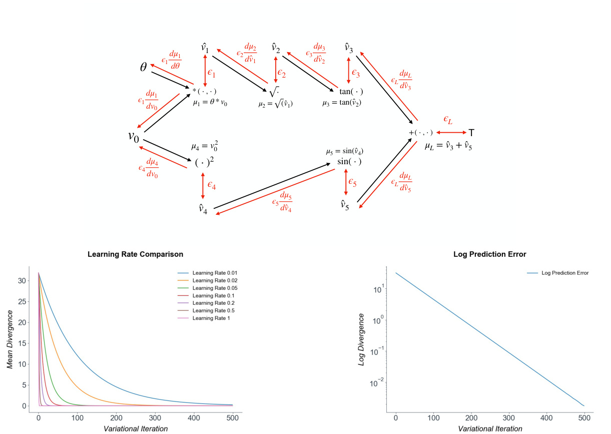
Figure 2: Top: The computation graph of the nonlinear test function $v_{L}=\tan(\sqrt{\theta v_{0}})+\sin(v_{0}^{2})$ . Bottom: graphs of the log mean divergence from the true gradient and the divergence for different learning rates. Convergence to the exact gradients is exponential and robust to high learning rates.
图 2: 上: 非线性测试函数 $v_{L}=\tan(\sqrt{\theta v_{0}})+\sin(v_{0}^{2})$ 的计算图。下: 不同学习率下对数平均散度与真实梯度的散度对比图。梯度收敛呈指数级且对高学习率具有鲁棒性。
4 Results
4 结果
4.1 Numerical Results
4.1 数值结果
To demonstrate the correctness of our derivation and empirical convergence to the true gradients, we present a numerical test in the simple scalar case, where we use predictive coding to derive the gradients of an arbitrary, highly nonlinear test function $v_{L}=\tan(\sqrt{\theta v_{0}})+\sin(v_{0}^{2})$ where $\theta$ is an arbitrary parameter. For our tests, we set $v_{0}$ to 5 and $\theta$ to 2. The computation graph for this function is presented in Figure 2. Although simple, this is a good test of predictive coding because the function is highly nonlinear, and its computation graph does not follow a simple layer structure but includes some branching. An arbitrary target of $T=3$ was set at the output and the gradient of the loss $L=(v_{L}-T)^{2}$ with respect to the input $v_{0}$ was computed by predictive coding. We show (Figure 2) that the predictive coding optimisation rapidly converges to the exact numerical gradients computed by automatic differentiation, and that moreover this optimization is very robust and can handle even exceptionally high learning rates (up to 0.5) without divergence.
为了验证我们推导的正确性以及经验性收敛到真实梯度的效果,我们在简单标量情况下进行了数值测试。该测试使用预测编码 (predictive coding) 推导任意高度非线性测试函数 $v_{L}=\tan(\sqrt{\theta v_{0}})+\sin(v_{0}^{2})$ 的梯度,其中 $\theta$ 为任意参数。测试中设定 $v_{0}=5$ 和 $\theta=2$,该函数的计算图如图 2 所示。虽然结构简单,但由于函数具有高度非线性且计算图不符合简单层级结构(包含分支),这对预测编码是很好的测试。我们在输出端设定任意目标值 $T=3$,并通过预测编码计算损失函数 $L=(v_{L}-T)^{2}$ 对输入 $v_{0}$ 的梯度。结果显示(图 2),预测编码优化能快速收敛至自动微分计算的精确数值梯度,且该优化过程具有极强鲁棒性,即使学习率高达 0.5 也不会发散。
In summary, we have shown and numerically verified that at the equilibrium point of the global free-energy $\mathcal{F}$ on an arbitrary computation graph, the error units exactly equal the back propagated gradients, and that this descent requires only local connectivity, does not require a separate phases or a sequential backwards sweep, and in the case of parameter-linear functions, requires only Hebbian plasticity. Our results provide a straightforward recipe for the direct implementation of predictive coding algorithms to approximate certain computation graphs, such as those found in common machine learning algorithms, in a biologically plausible manner. Next, we showcase this capability by developing predictive coding variants of core machine learning architectures - convolutional neural networks (CNNs) recurrent neural networks (RNNs) and LSTMs (Hochreiter & Schmid huber, 1997), and show performance comparable with backprop on tasks substantially more challenging than MNIST2.
总之,我们通过数值验证表明:在任意计算图上全局自由能 $\mathcal{F}$ 的平衡点处,误差单元完全等同于反向传播梯度,且该下降过程仅需局部连接性,无需独立相位或顺序反向扫描,对于参数线性函数仅需赫布可塑性。我们的研究结果为直接实现预测编码算法提供了简明方案,能以生物合理的方式近似特定计算图(如常见机器学习算法中的结构)。接着,我们通过开发核心机器学习架构的预测编码变体——卷积神经网络 (CNNs) 、循环神经网络 (RNNs) 和长短期记忆网络 (Hochreiter & Schmidhuber, 1997 [20]) ,在比MNIST2更具挑战性的任务上展示了与反向传播相当的性能。
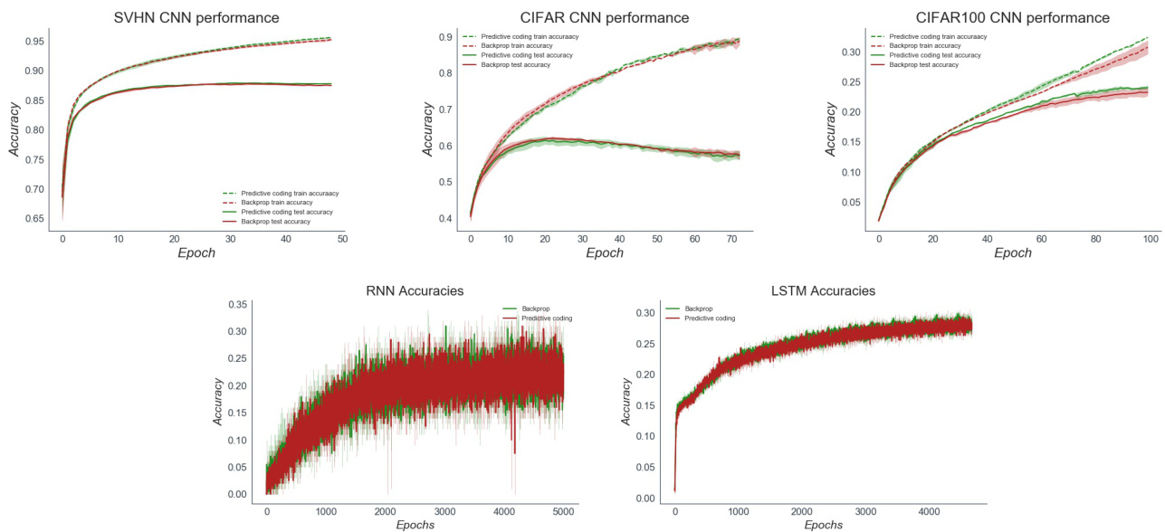
Figure 3: Top Row: Training and test accuracy plots for the predictive coding and backprop CNN on SVHN,CIFAR10, and CIFAR10 dataest over 5 seeds. Bottom row: Training and test accuracy plots for the predictive coding and backprop RNN and LSTM. Performance is largely indistinguishable. Due to the need to iterate the vs until convergence, the predictive coding network had roughly a $100\mathrm{x}$ greater computational cost than the backprop network.
图 3: 上排: 预测编码 (predictive coding) 和反向传播 (backprop) CNN 在 SVHN、CIFAR10 和 CIFAR10 数据集上经过 5 次随机种子运行的训练与测试准确率曲线。下排: 预测编码和反向传播 RNN 及 LSTM 的训练与测试准确率曲线。两者性能基本无法区分。由于需要迭代直至收敛,预测编码网络的计算成本约为反向传播网络的 $100\mathrm{x}$ 倍。
4.2 Predictive Coding CNN, RNN, and LSTM
4.2 预测编码 CNN、RNN 和 LSTM
First, we constructed predictive coding CNN models (see Appendix B for full implementation details). In the predictive coding CNN, each filter kernel was augmented with ’error maps’ which measured the difference between the forward convolutional predictions and the backwards messages. Our CNN was composed of a convolutional layer, followed by a max-pooling layer, then two further convolutional layers followed by 3 fully-connected layers. We compared our predictive coding CNN to a backprop-trained CNN with the exact same architecture and hyper parameters. We tested our models on three image classification datasets significantly more challenging than MNIST – SVHN, CIFAR10, and CIFAR100. SVHN is a digit recognition task like MNIST, but has more naturalistic backgrounds, is in colour with continuously varying inputs and contains distractor digits. CIFAR10 and CIFAR100 are large image datasets composed of RGB $32\mathbf{x}32$ images. CIFAR10 has 10 classes of image, while CIFAR100 is substantially more challenging with 100 possible classes. In general, performance was identical between the predictive coding and backprop CNNs and comparable to the standard performance of basic CNN models on these datasets, Moreover, the predictive coding gradient remained close to the true numerical gradient throughout training.
首先,我们构建了预测编码CNN模型(完整实现细节见附录B)。在该模型中,每个滤波器核都配备了"误差图"来测量前向卷积预测与反向消息之间的差异。我们的CNN结构包含一个卷积层、一个最大池化层、两个后续卷积层以及3个全连接层。我们将该预测编码CNN与采用完全相同架构和超参数的反向传播训练CNN进行对比,在比MNIST更具挑战性的三个图像分类数据集(SVHN、CIFAR10和CIFAR100)上进行测试。SVHN是与MNIST类似的数字识别任务,但具有更自然的背景、连续变化的彩色输入及干扰数字。CIFAR10和CIFAR100是由RGB $32\mathbf{x}32$图像组成的大型数据集,其中CIFAR10包含10个类别,而CIFAR100具有100个类别因而更具挑战性。实验表明,预测编码CNN与反向传播CNN性能相当,均达到基础CNN模型在这些数据集上的标准水平,且预测编码梯度在整个训练过程中始终接近真实数值梯度。
We also constructed predictive coding RNN and LSTM models, thus demonstrating the ability of predictive coding to scale to non-parameter-linear, branching, computation graphs. The RNN was trained on a character-level name classification task, while the LSTM was trained on a next-character prediction task on the full works of Shakespeare. Full implementation details can be found in Appendices B and C. LSTMs and RNNs are recurrent networks which are trained through back propagation through time (BPTT). BPTT simply unrolls the network through time and back propagates through the unrolled graph. Analogously we trained the predictive coding RNN and LSTM by applying predictive coding to the unrolled computation graph. The depth of the unrolled graph depends heavily on the sequence length, and in our tasks using a sequence length of 100 we still found that predictive coding evinced rapid convergence to the correct numerical gradient, thus showing that the algorithm is scalable even to very deep computation graphs.
我们还构建了预测编码(predictive coding)RNN和LSTM模型,从而证明预测编码能够扩展到非线性参数、分支化的计算图结构。其中RNN在字符级人名分类任务上进行训练,而LSTM则在莎士比亚全集的下一个字符预测任务上进行训练。完整实现细节见附录B和C。
LSTM和RNN都是通过时间反向传播(BPTT)训练的循环网络。BPTT本质上是将网络在时间维度上展开,并通过展开后的计算图进行反向传播。类似地,我们通过对展开后的计算图应用预测编码来训练预测编码RNN和LSTM。展开图的深度与序列长度密切相关,在我们采用100个时间步长的任务中,预测编码仍能快速收敛到正确的数值梯度,这表明该算法甚至能扩展到极深度的计算图结构。
5 Discussion
5 讨论
We have shown that predictive coding provides a local and often biologically plausible approximation to backprop on arbitrary, deep, and branching computation graphs. Moreover, convergence to the exact backprop gradients is rapid and robust, even in extremely deep graphs such as the unrolled LSTM. Our algorithm is fully parallel iz able, does not require separate phases, and can produce equivalent performance to backprop in core machine-learning architectures. These results broaden the horizon of local approximations to backprop by demonstrating that they can be implemented on arbitrary computation graphs, not only simple MLP architectures. Our work prescribes a straightforward recipe for back propagating through any computation graph with predictive coding using only local learning rules. In the future, this process could potentially be made fully automatic and translated onto neuro m orphic hardware. Our results also raise the possibility that the brain may implement machine-learning type architectures much more directly than often considered. Many lines of work suggest a close correspondence between the representations and activation s of CNNs and activity in higher visual areas (Eickenberg, Gramfort, Varoquaux, & Thirion, 2017; Khaligh-Razavi & Krieg esko rte, 2014; Lindsay, 2020; Tacchetti, Isik, & Poggio, 2017; Yamins et al., 2014), for instance, and this similarity may be found to extend to other machine learning architectures.
我们证明了预测编码(predictive coding)为任意深度分支计算图上的反向传播(backprop)提供了一种局部且通常具有生物学合理性的近似方法。此外,即使在展开LSTM等极深计算图中,该方法也能快速稳健地收敛至精确的反向传播梯度。我们的算法完全可并行化,无需分阶段运行,并能在核心机器学习架构中实现与反向传播等效的性能。这些成果通过证明局部近似方法可应用于任意计算图(而不仅限于简单多层感知机架构),拓宽了反向传播局部近似的研究视野。本研究为通过预测编码实现任意计算图的反向传播提供了一套仅使用局部学习规则的简明方案。未来,该流程有望实现全自动化并移植至神经形态硬件。我们的发现还提出了另一种可能性:大脑可能以比通常认为的更直接方式实现机器学习类架构。例如,大量研究表明CNN的表征和激活模式与高级视觉区域活动高度吻合 [20][21][22][23][24],这种相似性可能同样存在于其他机器学习架构中。
Although we have implemented three core machine learning architectures as predictive coding networks, we have nevertheless focused on relatively small and straightforward networks and thus both our backprop and predictive coding networks perform below the state of the art on the presented tasks. This is primarily because our focus was on demonstrating the theoretical convergence between the two algorithms. Nevertheless, we believe that due to the generality of our theoretical results, ’scaling up’ the existing architectures to implement performance-matched predictive coding versions of more advanced machine learning architectures such as resnets (He, Zhang, Ren, & Sun, 2016), GANs (Goodfellow et al., 2014), and transformers (Vaswani et al., 2017) should be relatively straightforward.
虽然我们已经将三种核心机器学习架构实现为预测编码网络,但仍聚焦于相对简单的小型网络,因此无论是反向传播还是预测编码网络在当前任务中的表现都未达到最优水平。这主要是因为我们的研究重点在于验证两种算法的理论收敛性。尽管如此,基于理论结果的普适性,我们相信将现有架构扩展为性能匹配的预测编码版本(例如残差网络 (He, Zhang, Ren, & Sun, 2016) 、生成对抗网络 (Goodfellow et al., 2014) 和 Transformer (Vaswani et al., 2017) 等先进机器学习架构)应具有较高的可行性。
In terms of computational cost, one inference iteration in the predictive coding network is about as costly as a backprop backwards pass. Thus, due to using 100-200 iterations for full convergence, our algorithm is substantially more expensive than backprop which limits the s cal ability of our method. However, this serial cost is misleading when talking about highly parallel neural architectures. In the brain, neurons cannot wait for a sequential forward and backward sweep. By phrasing our algorithm as a global descent, our algorithm is fully parallel across layers. There is no waiting and no phases to be coordinated. Each neuron need only respond to its local driving inputs and downwards error signals. We believe that this local and parallel iz able property of our algorithm may engender the possibility of substantially more efficient implementations on neuro m orphic hardware (Davies et al., 2018; Furber, Galluppi, Temple, & Plana, 2014; Merolla et al., 2014), which may ameliorate much of the computational overhead compared to backprop. Future work could also examine whether our method is more capable than backprop of handling the continuously varying inputs the brain is presented with in practice, rather than the artificial paradigm of being presented with a series of i.i.d. datapoints.
在计算成本方面,预测编码网络中的一次推理迭代与反向传播(backprop)的反向传递成本相当。因此,由于需要100-200次迭代才能完全收敛,我们的算法比反向传播昂贵得多,这限制了方法的可扩展性。然而,在讨论高度并行的神经架构时,这种串行成本具有误导性。在大脑中,神经元无法等待顺序的前向和后向传递。通过将我们的算法表述为全局下降,我们的算法在各层之间完全并行。无需等待,也无需协调阶段。每个神经元只需响应其局部驱动输入和向下误差信号。我们认为,我们算法的这种局部且可并行化的特性可能为神经形态硬件(Davies等人,2018;Furber、Galluppi、Temple和Plana,2014;Merolla等人,2014)上实现更高效的实现提供可能性,从而相比反向传播大幅改善计算开销。未来的工作还可以研究我们的方法是否比反向传播更能处理大脑在实际中遇到的连续变化输入,而不是处理一系列独立同分布(i.i.d.)数据点的人工范式。
Our work also reveals a close connection between backprop and inference. Namely, the recursive computation of gradients is effectively a by-product of a variation al-inference algorithm which infers the values of the vertices of the computation graph under a hierarchical Gaussian generative model. While the deep connections between stochastic gradient descent and inference in terms of Kalman filtering (Ollivier, 2019; Ruck, Rogers, Kabrisky, Maybeck, & Oxley, 1992) or MCMC sampling methods (T. Chen, Fox, & Guestrin, 2014; Mandt, Hoffman, & Blei, 2017) is known, the relation between recursive gradient computation itself and variation al inference is under explored except in the case of a single layer (Amari, 1995). Our method can provide a principled generalisation of backprop through the inverse-variance $\Sigma^{-1}$ parameters of the Gaussian generative model. These parameters weight the relative contribution of different factors to the overall gradient by their uncertainty, thus naturally handling the case of backprop with differential ly noisy inputs. Moreover, the $\Sigma^{-1}$ parameters can be learnt as a gradient descent on $\mathcal{F}$ : $\begin{array}{r}{\frac{d\Sigma_{i}}{d t}=-\frac{d\mathcal{F}}{d\Sigma_{i}}=-\Sigma_{i}^{-1}\epsilon_{i}\epsilon_{i}^{T}\Sigma_{i}^{-1}-\Sigma_{i}^{-1}}\end{array}$ . This specific generalisation is afforded by the Gaussian form of the generative model, however, and other generative models may yield novel optimisation algorithms able to quantify and handle uncertainties throughout the entire computational graph.
我们的研究还揭示了反向传播与推断之间的紧密联系。具体而言,梯度的递归计算本质上是变分推断算法的一个副产品,该算法在分层高斯生成模型下推断计算图顶点的值。虽然随机梯度下降与卡尔曼滤波 [Ollivier, 2019; Ruck, Rogers, Kabrisky, Maybeck, & Oxley, 1992] 或MCMC采样方法 [T. Chen, Fox, & Guestrin, 2014; Mandt, Hoffman, & Blei, 2017] 之间的深刻联系已被认知,但递归梯度计算本身与变分推断的关系除单层情况外 [Amari, 1995] 仍缺乏探索。我们的方法通过高斯生成模型的逆方差$\Sigma^{-1}$参数,为反向传播提供了原则性的推广。这些参数根据不确定性加权不同因素对整体梯度的相对贡献,从而自然处理输入存在差分噪声的反向传播情况。此外,$\Sigma^{-1}$参数可通过$\mathcal{F}$的梯度下降学习:$\begin{array}{r}{\frac{d\Sigma_{i}}{d t}=-\frac{d\mathcal{F}}{d\Sigma_{i}}=-\Sigma_{i}^{-1}\epsilon_{i}\epsilon_{i}^{T}\Sigma_{i}^{-1}-\Sigma_{i}^{-1}}\end{array}$。这种特定推广得益于生成模型的高斯形式,但其他生成模型可能产生能够量化和处理整个计算图中不确定性的新型优化算法。
Acknowledgements
致谢
BM is supported by an EPSRC funded PhD Studentship. AT is funded by a PhD studentship from the Dr. Mortimer and Theresa Sackler Foundation and the School of Engineering and Informatics at the University of Sussex. CLB is supported by BBRSC grant number BB/P022197/1 and by Joint Research with the National Institutes of Natural Sciences (NINS), Japan, program No. 01112005. AT is grateful to the Dr. Mortimer and Theresa Sackler Foundation, which supports the Sackler Centre for Consciousness Science.
BM由英国工程与物理科学研究委员会(EPSRC)资助的博士奖学金支持。AT的博士研究由Dr. Mortimer and Theresa Sackler基金会与萨塞克斯大学工程与信息学院联合资助。CLB获得英国生物技术与生物科学研究委员会(BBRSC)资助(编号BB/P022197/1)及日本自然科学研究机构(NINS)联合研究项目(编号01112005)支持。AT感谢Dr. Mortimer and Theresa Sackler基金会对Sackler意识科学中心的资助。
References
参考文献
Appendix A: Predictive Coding CNN Implementation Details
附录 A: 预测编码 CNN 实现细节
The key concept in a CNN is that of an image convolution, where a small weight matrix is ’slid’ (or convolved) across an image to produce an output image. Each patch of the output image only depends on a relatively small patch of the input image. Moreover, the weights of the filter stay the same during the convolution, so each pixel of the output image is generated using the same weights. The weight sharing implicit in the convolution operation enforces translational invariance, since different image patches are all processed with the same weights.
CNN的核心概念是图像卷积 (image convolution),即通过一个小型权重矩阵在图像上"滑动"(或卷积)来生成输出图像。输出图像的每个局部区域仅依赖于输入图像相对较小的局部区域。此外,卷积过程中滤波器的权重保持不变,因此输出图像的每个像素都是使用相同权重生成的。卷积操作中隐含的权重共享机制实现了平移不变性 (translational invariance),因为所有图像局部区域都使用相同权重进行处理。
The forward equations of a convolutional layer for a specific output pixel
特定输出像素的卷积层前向方程
$$
v_{i,j}=\sum_{k=i-f}^{k=i+f}\sum_{l=j-f}^{l=j+f}\theta_{k,l}x_{i+k,j+l}
$$
$$
v_{i,j}=\sum_{k=i-f}^{k=i+f}\sum_{l=j-f}^{l=j+f}\theta_{k,l}x_{i+k,j+l}
$$
Where $v_{i,j}$ is the $(i,j)$ th element of the output, $x_{i,j}$ is the element of the input image and $\theta_{k,l}$ is an weight element of a feature map. To setup a predictive coding CNN, we augment each intermediate $x_{i}$ and $v_{i}$ with error units $\epsilon_{i}$ of the same dimension as the output of the convolutional layer.
其中 $v_{i,j}$ 是输出的第 $(i,j)$ 个元素,$x_{i,j}$ 是输入图像的元素,$\theta_{k,l}$ 是特征图的权重元素。为构建预测编码 CNN (Convolutional Neural Network) ,我们在每个中间层 $x_{i}$ 和 $v_{i}$ 上添加了与卷积层输出维度相同的误差单元 $\epsilon_{i}$ 。
Predictions $\hat{v}$ are projected forward using the forward equations. Prediction errors also need to be transmitted backwards for the architecture to work. To achieve this we must have that prediction errors are transmitted upwards by a ’backwards convolution’. We thus define the backwards prediction errors $\hat{\epsilon}_{j}$ as follows:
预测值 $\hat{v}$ 通过前向方程进行前向投影。预测误差也需要反向传播以使架构正常工作。为此,我们必须通过"反向卷积"向上传递预测误差。因此,我们将反向预测误差 $\hat{\epsilon}_{j}$ 定义如下:
$$
\hat{\epsilon}_ {i,j}=\sum_{k=i-f}^{i+f}\sum_{l=j-f}^{j+f}\theta_{j,i}\tilde{\epsilon}_{i,j}
$$
$$
\hat{\epsilon}_ {i,j}=\sum_{k=i-f}^{i+f}\sum_{l=j-f}^{j+f}\theta_{j,i}\tilde{\epsilon}_{i,j}
$$
Where is an error map zero-padded to ensure the correct convolutional output size. Inference in the predictive coding network then proceeds by updating the intermediate values of each layer as follows:
其中 是一个经过零填充以确保正确卷积输出尺寸的误差图。预测编码网络的推理过程通过按以下方式更新每层的中间值来实现:
$$
\frac{d v_{l}}{d t}=\epsilon_{l}-\hat{\epsilon}_{l+1}
$$
$$
\frac{d v_{l}}{d t}=\epsilon_{l}-\hat{\epsilon}_{l+1}
$$
Since the CNN is also parameter-linear, weights can be updated using the simple Hebbian rule of the multiplication of the pre and post synaptic potentials.
由于 CNN 也是参数线性的,权重可以通过简单的赫布规则 (Hebbian rule) 进行更新,即突触前后电位的乘积。
$$
\frac{d\theta_{l}}{d t}=\sum_{i,j}\epsilon_{l_{i,j}}v_{l-1_{i,j}}T_{}
$$
$$
\frac{d\theta_{l}}{d t}=\sum_{i,j}\epsilon_{l_{i,j}}v_{l-1_{i,j}}T_{}
$$
There is an additional biological implausibility here due to the weight sharing of the CNN. Since the same weights are copied for each position on the image, the weight updates have contributions from all aspects of the image simultaneously which violates the locality condition. A simple fix for this, which makes the network scheme plausible is to simply give each position on the image a filter with separate weights, thus removing the weight sharing implicit in the CNN. In effect this gives each patch of pixels a local receptive field with its own set of weights. The performance and s cal ability of such a locally connected predictive coding architecture would be an interesting avenue for future work, as this architecture has substantial homologies with the structure of the visual cortex.
由于CNN(卷积神经网络)的权重共享机制,这里还存在一个生物学上的不合理性。由于图像每个位置都复制相同的权重,权重更新会同时受到图像所有区域的影响,这违背了局部性原则。一个简单的改进方案是让图像每个位置都拥有独立权重的滤波器,从而消除CNN隐含的权重共享机制。这实际上为每个像素块提供了具有独立权重组的局部感受野。这种局部连接的预测编码架构在性能与可扩展性方面的表现将是一个值得探索的研究方向,因为该架构与视觉皮层结构存在高度同源性[20]。
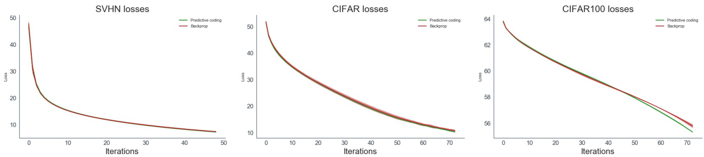
Figure 4: Training loss plots for the Predictive Coding and Backprop CNN on SVHN,CIFAR10, and CIFAR10 dataest over 5 seeds.
图 4: 在SVHN、CIFAR10和CIFAR10数据集上经过5次随机种子训练的预测编码(Predictive Coding)与反向传播(Backprop)CNN的训练损失曲线。
In our experiments we used a relatively simple CNN architecture consisting of one convolutional layer of kernel size 5, and a filter bank of 6 filters. This was followed by a max-pooling layer with a (2,2) kernel and a further convolutional layer with a (5,5) kernel and filter bank of 16 filters. This was then followed by three fully connected layers of 200, 150, and 10 (or 100 for CIFAR100) output units. Although this architecture is far smaller than state of the art for convolutional networks, the primary point of our paper was to demonstrate the equivalence of predictive coding and backprop. Further work could investigate scaling up predictive coding to more state-of-the-art architectures.
在我们的实验中,我们使用了一个相对简单的CNN架构,包含一个核大小为5的卷积层和一个由6个滤波器组成的滤波器组。随后是一个核大小为(2,2)的最大池化层,以及另一个核大小为(5,5)、滤波器组包含16个滤波器的卷积层。之后是三个全连接层,分别有200、150和10(对于CIFAR100数据集则为100)个输出单元。虽然这一架构远小于卷积网络的最先进水平,但我们论文的主要目的是证明预测编码(predictive coding)与反向传播(backprop)的等价性。后续工作可以研究将预测编码扩展到更先进的架构中。
Our datasets consisted of $32\mathbf{x}32$ RGB images. We normalised the values of all pixels of each image to lie between 0 and 1, but otherwise performed no other image preprocessing. We did not use data augmentation of any kind. We set the weight learning rate for the predictive coding and backprop networks 0.0001. A minibatch size of 64 was used. These parameters were chosen without any detailed hyper parameter search and so are likely suboptimal. The magnitude of the gradient updates was clamped to lie between -50 and 50 in all of our models. This was done to prevent divergences, as occasionally occurred in the LSTM networks, likely due to exploding gradients.
我们的数据集由 $32\mathbf{x}32$ RGB图像组成。我们将每张图像所有像素值归一化到0至1范围内,除此之外未进行其他图像预处理。未采用任何形式的数据增强。预测编码网络和反向传播网络的权重学习率均设为0.0001,使用64的小批量(minibatch)大小。这些参数未经详细超参数搜索选定,因此可能非最优解。所有模型中梯度更新的幅度被限制在-50到50之间,此举旨在防止LSTM网络中偶尔因梯度爆炸导致的发散现象。
The predictive coding scheme converged to the exact backprop gradients very precisely within 100 inference iterations using an inference learning rate of 0.1. This gives the predictive coding CNN approximately a $100\mathbf{x}$ computational overhead compared to backprop. The divergence between the true and approximate gradients remained approximately constant throughout training, as shown by Figure 5, which shows the mean divergence for each layer of the CNN over the course of an example training run on the CIFAR10 dataset. The training loss of the predictive coding and backprop networks for SVHN, CIFAR10 and CIFAR100 are presented in Figure 4.
预测编码方案在使用0.1推理学习率的情况下,经过100次推理迭代后非常精确地收敛到与反向传播完全相同的梯度。这使得预测编码CNN相比反向传播产生了约$100\mathbf{x}$的计算开销。如图5所示,在整个训练过程中,真实梯度与近似梯度之间的差异保持基本恒定,该图展示了CNN各层在CIFAR10数据集训练过程中的平均差异。预测编码网络与反向传播网络在SVHN、CIFAR10和CIFAR100数据集上的训练损失如图4所示。
Appendix B: Predictive Coding RNN
附录 B: 预测编码循环神经网络 (Predictive Coding RNN)
The computation graph on RNNs is relatively straightforward. We consider only a single layer RNN here although the architecture can be straightforwardly extended to hierarchically stacked RNNs. An RNN is similar to a feed forward network except that it possesses an additional hidden state $h$ which is maintained and updated over time as a function of both the current input $x$ and the previous hidden state. The output of the network $y$ is a function of $h$ . By considering the RNN at a single timestep we obtain the following equations.
RNN的计算图相对简单。这里我们仅考虑单层RNN,不过该架构可以轻松扩展到层级堆叠的RNN。RNN与前馈网络类似,区别在于它拥有一个额外的隐藏状态$h$,该状态会随时间推移而更新,其值由当前输入$x$和前一个隐藏状态共同决定。网络输出$y$则是$h$的函数。通过观察RNN在单个时间步的表现,我们得到以下方程。
$$
\begin{array}{l}{{h_{t}}=f{({\theta_{h}}{h_{t-1}}+{\theta_{x}}{x_{t}})}}\ {{y_{t}}=g{({\theta_{y}}{h_{t}})}}\end{array}
$$
$$
\begin{array}{l}{{h_{t}}=f{({\theta_{h}}{h_{t-1}}+{\theta_{x}}{x_{t}})}}\ {{y_{t}}=g{({\theta_{y}}{h_{t}})}}\end{array}
$$
Where f and $\mathrm{g}$ are element wise nonlinear activation functions. And $\theta_{h},\theta_{x},\theta_{y}$ are weight matrices for each specific input. To predict a sequence the RNN simply rolls forward the above equations to generate new predictions and hidden states at each timestep.
其中f和$\mathrm{g}$是逐元素的非线性激活函数,$\theta_{h}$、$\theta_{x}$、$\theta_{y}$则是各输入对应的权重矩阵。RNN通过前向展开上述方程,在每一时间步生成新预测和隐藏状态来实现序列预测。
RNNs are typically trained through an algorithm called back propagation through time (BPTT) which essentially just unrolls the RNN into a single feed forward computation graph and then performs back propagation through this unrolled graph. To train the RNN using predictive coding we take the same approach and simply apply predictive coding to the unrolled graph.
RNN通常通过一种称为随时间反向传播(BPTT)的算法进行训练,该算法本质上是将RNN展开为单一前馈计算图,然后通过这个展开图执行反向传播。为了使用预测编码训练RNN,我们采用相同的方法,只需将预测编码应用于展开图。
It is important to note that this is an additional aspect of biological implausibility that we do not address in this paper. BPTT requires updates to proceed backwards through time from the end of the sequence to the beginning. Ignoring any biological implausibility with the rules themselves, this updating sequence is clearly not biologically plausible as naively it requires maintaining the entire sequence of predictions and prediction errors perfectly in memory until the end of the sequence, and waiting until the sequence ends before making any updates. There is a small literature on trying to produce biologically plausible, or forward-looking approximations to BPTT which does not require updates to be propagated back through time (Lillicrap & Santoro, 2019; Ollivier, Tallec, & Charpiat, 2015; Steil, 2004; Tallec & Ollivier, 2017; Williams & Zipser, 1989). While this is a fascinating area, we do not address it in this paper. We are solely concerned with the fact that predictive coding approximates back propagation on feed forward computation graphs for which the unrolled RNN graph is a sufficient substrate.
需要注意的是,这是我们未在本文中解决的生物合理性问题的另一个方面。BPTT (Backpropagation Through Time) 要求更新从序列末端向起始端逆向进行。即便忽略规则本身的生物不合理性,这种更新顺序显然也不符合生物机制——因为从直观上看,它需要将整个预测序列和预测误差完美保存在记忆中直至序列结束,并且必须等待序列完成后才能执行任何更新。现有少量研究尝试构建生物合理性或前向近似的BPTT方法,这些方法无需随时间反向传播更新 (Lillicrap & Santoro, 2019; Ollivier, Tallec, & Charpiat, 2015; Steil, 2004; Tallec & Ollivier, 2017; Williams & Zipser, 1989)。尽管这是个引人入胜的领域,但本文不予探讨。我们仅关注预测编码 (predictive coding) 在前向计算图(其中展开的RNN图是充分载体)上近似反向传播这一事实。
To learn a predictive coding RNN, we first augment each of the variables $h_{t}$ and $y_{t}$ of the original graph with additional error units $\epsilon_{h_{t}}$ and $\epsilon_{y_{t}}$ . Predictions $\hat{y}_ {t},\hat{h}_ {t}$ are generated according to the feed forward rules (16). A sequence of true labels ${T_{1}...T_{T}}$ is then presented to the network, and then inference proceeds by recursively applying the following
为了学习预测编码循环神经网络 (RNN),我们首先在原始图的每个变量 $h_{t}$ 和 $y_{t}$ 上增加额外的误差单元 $\epsilon_{h_{t}}$ 和 $\epsilon_{y_{t}}$。预测值 $\hat{y}_ {t},\hat{h}_ {t}$ 根据前馈规则 (16) 生成。随后向网络输入一系列真实标签 ${T_{1}...T_{T}}$,并通过递归应用以下规则进行推理:

Figure 5: Mean divergence between the true numerical and predictive coding backprops over the course of training. In general, the divergence appeared to follow a largely random walk pattern, and was generally neglible. Importantly, the divergence did not grow over time throughout training, implying that errors from slightly incorrect gradients did not appear to compound.
图 5: 训练过程中真实数值反向传播与预测编码反向传播之间的平均差异。总体而言,差异基本呈现随机游走模式且可忽略不计。关键的是,差异并未随训练时间增长而扩大,这表明轻微梯度误差不会产生累积效应。
rules backwards through time until convergence.
规则逆向传播直至收敛。
$$
\begin{array}{c}{{\epsilon_{y_{t}}=L-\hat{y}_ {t}}}\ {{\epsilon_{h_{t}}=h_{t}-\hat{h}_ {t}}}\ {{\displaystyle\frac{d h_{t}}{d t}=\epsilon_{h_{t}}-\epsilon_{y_{t}}\theta_{y}^{T}-\epsilon_{h_{t+1}}\theta_{h}^{T}}}\end{array}
$$
$$
\begin{array}{c}{{\epsilon_{y_{t}}=L-\hat{y}_ {t}}}\ {{\epsilon_{h_{t}}=h_{t}-\hat{h}_ {t}}}\ {{\displaystyle\frac{d h_{t}}{d t}=\epsilon_{h_{t}}-\epsilon_{y_{t}}\theta_{y}^{T}-\epsilon_{h_{t+1}}\theta_{h}^{T}}}\end{array}
$$
Upon convergence the weights are updated according to the following rules.
权重更新遵循以下规则收敛后执行。
$$
\begin{array}{l}{\displaystyle\frac{d\theta_{y}}{d t}=\sum_{t=0}^{T}\epsilon_{y t}\frac{\partial g(\theta_{y}h_{t})}{\partial\theta_{y}}h_{t}^{T}}\ {\displaystyle\frac{d\theta_{x}}{d t}=\sum_{t=0}^{T}\epsilon_{h_{t}}\frac{\partial f(\theta_{h}h_{t-1}+\theta_{x}x_{t})}{\partial\theta_{x}}x_{t}^{T}}\ {\displaystyle\frac{d\theta_{h}}{d t}=\sum_{t=0}^{T}\epsilon_{h_{t}}\frac{\partial f(\theta_{h}h_{t-1}+\theta_{x}x_{t})}{\partial\theta_{h}}h_{t+1}^{T}}\end{array}
$$
$$
\begin{array}{l}{\displaystyle\frac{d\theta_{y}}{d t}=\sum_{t=0}^{T}\epsilon_{y t}\frac{\partial g(\theta_{y}h_{t})}{\partial\theta_{y}}h_{t}^{T}}\ {\displaystyle\frac{d\theta_{x}}{d t}=\sum_{t=0}^{T}\epsilon_{h_{t}}\frac{\partial f(\theta_{h}h_{t-1}+\theta_{x}x_{t})}{\partial\theta_{x}}x_{t}^{T}}\ {\displaystyle\frac{d\theta_{h}}{d t}=\sum_{t=0}^{T}\epsilon_{h_{t}}\frac{\partial f(\theta_{h}h_{t-1}+\theta_{x}x_{t})}{\partial\theta_{h}}h_{t+1}^{T}}\end{array}
$$
Since the RNN feed forward updates are parameter-linear, these rules are Hebbian, only requiring the multiplication of pre and post-synaptic potentials. This means that the predictive coding updates proposed here are biologically plausible and could in theory be implemented in the brain. The only biological implausibility remains the BPTT learning scheme.
由于RNN的前馈更新是参数线性的,这些规则具有赫布性(Hebbian),仅需突触前后电位的乘积运算。这意味着本文提出的预测编码更新机制具有生物学合理性,理论上可在大脑中实现。唯一不符合生物学特性的部分仍是BPTT(Backpropagation Through Time)学习机制。
Our RNN was trained on a simple character-level name-origin dataset which can be found here: https://download.pytorch.org/tutorial/data.zip. The RNN was presented with sequences of characters representing names and had to predict the national origin of the name – French, Spanish, Russian, etc. The characters were presented to the network as one-hot-encoded vectors without any embedding. The output categories were also presented as a one-hot vector. The RNN has a hidden size of 256 units. A tanh non linearity was used between hidden states and the output layer was linear. The network was trained on randomly selected name-category pairs from the dataset. The training loss for the predictive coding and backprop RNNs, averaged over 5 seeds is presented below (Figure 6).
我们的RNN在一个简单的字符级姓名-来源数据集上进行了训练,该数据集可在此处获取:https://download.pytorch.org/tutorial/data.zip。RNN接收表示姓名的字符序列,并需要预测姓名的国籍——法国、西班牙、俄罗斯等。字符以独热编码(one-hot-encoded)向量形式输入网络,未进行任何嵌入处理。输出类别同样以独热向量形式呈现。该RNN的隐藏层大小为256单元,隐藏状态间使用tanh非线性函数,输出层为线性层。网络训练时随机从数据集中选取姓名-类别对进行学习。预测编码和反向传播RNN的训练损失(基于5次随机种子的平均值)如下所示(图6)。

Figure 6: Training losses for the predictive coding and backprop RNN. As expected, they are effectively identical.
图 6: 预测编码(predictive coding)与反向传播RNN的训练损失对比。正如预期所示,两者基本完全一致。
Appendix C: Predictive Coding LSTM Implementation Details
附录 C: 预测编码 LSTM 实现细节
Unlike the other two models, the LSTM possesses a complex and branching internal computation graph, and is thus a good opportunity to make explicit the predictive coding ’recipe’ for approximating backprop on arbitrary computation graphs. The computation graph for a single LSTM cell is shown (with backprop updates) in Figure 7. Prediction for the LSTM occurs by simply rolling forward a copy of the LSTM cell for each timestep. The LSTM cell receives its hidden state $h_{t}$ and cell state $c_{t}$ from the previous timestep. During training we compute derivatives on the unrolled computation graph and receive backwards derivatives (or prediction errors) from the LSTM cell at time $t+1$ .
与其他两种模型不同,LSTM (Long Short-Term Memory) 拥有复杂且分叉的内部计算图,因此是展示预测编码 (predictive coding) 如何近似任意计算图上反向传播的绝佳案例。单个LSTM单元的计算图(含反向传播更新)如图7所示。LSTM的预测过程只需在每个时间步向前滚动一个LSTM单元副本即可。该单元接收来自前一时间步的隐藏状态 $h_{t}$ 和细胞状态 $c_{t}$。训练时,我们在展开的计算图上计算导数,并从 $t+1$ 时刻的LSTM单元接收反向导数(即预测误差)。

Figure 7: Computation graph and backprop learning rules for a single LSTM cell.
图 7: 单个LSTM单元的计算图及反向传播学习规则。
The equations that specify the computation graph of the LSTM cell are as follows.
指定LSTM单元计算图的公式如下。
$$
\begin{array}{r l}&{v_{1}=h_{t}\oplus x_{t}}\ &{v_{2}=\sigma(\theta_{i}v_{1})}\ &{v_{3}=c_{1}v_{2}}\ &{v_{4}=\sigma(\theta_{i\operatorname*{in}}v_{1})}\ &{v_{5}=\operatorname{tanh}(\theta_{e}v_{1})}\ &{v_{6}=v_{4}v_{5}}\ &{v_{7}=v_{3}+v_{6}}\ &{v_{8}=\sigma(\theta_{e}v_{1})}\ &{v_{9}=\operatorname{tanh}(v_{7})}\ &{\tau_{10}=v_{8}v_{9}}\ &{y_{1}=\sigma(\theta_{8}v_{10})}\ &{y_{9}=\sigma(\theta_{8}v_{10})}\ &{y_{10}=\sigma(\theta_{8}v_{10})}\end{array}
$$
$$
\begin{array}{r l}&{v_{1}=h_{t}\oplus x_{t}}\ &{v_{2}=\sigma(\theta_{i}v_{1})}\ &{v_{3}=c_{1}v_{2}}\ &{v_{4}=\sigma(\theta_{i\operatorname*{in}}v_{1})}\ &{v_{5}=\operatorname{tanh}(\theta_{e}v_{1})}\ &{v_{6}=v_{4}v_{5}}\ &{v_{7}=v_{3}+v_{6}}\ &{v_{8}=\sigma(\theta_{e}v_{1})}\ &{v_{9}=\operatorname{tanh}(v_{7})}\ &{\tau_{10}=v_{8}v_{9}}\ &{y_{1}=\sigma(\theta_{8}v_{10})}\ &{y_{9}=\sigma(\theta_{8}v_{10})}\ &{y_{10}=\sigma(\theta_{8}v_{10})}\end{array}
$$
The recipe to convert this computation graph into a predictive coding algorithm is straightforward. We first rewire the connectivity so that the predictions are set to the forward functions of their parents. We then compute the errors
将计算图转换为预测编码算法的方案很直接。首先重新连接节点,使预测值等于其父节点的前向函数值,随后计算误差
between the vertices and the predictions.
顶点与预测之间的关系。

During inference, the inputs $h_{t},x_{t}$ and the output $y_{t}$ are fixed. The vertices and then the prediction errors are updated according to Equation 2. This recipe is straightforward and can easily be extended to other more complex machine learning architectures. The full augmented computation graph, including the vertex update rules, is presented in Figure 8.
在推理过程中,输入 $h_{t},x_{t}$ 和输出 $y_{t}$ 是固定的。根据公式2更新顶点和预测误差。这种方法简单直接,可以轻松扩展到其他更复杂的机器学习架构。完整的增强计算图(包括顶点更新规则)如图8所示。
Empirically, we observed rapid convergence to the exact backprop gradients even in the case of very deep computation graphs (as is an unrolled LSTM with a sequence length of 100). Although convergence was slower than was the case for CNNs or lesser sequence lengths, it was still straightforward to achieve convergence to the exact numerical gradients with sufficient iterations.
从实验观察来看,即便在极深计算图(如序列长度为100的展开LSTM)的情况下,我们仍能快速收敛至精确的反向传播梯度。虽然其收敛速度较CNN或较短序列的情况更慢,但通过足够迭代次数仍可轻松实现与精确数值梯度的收敛。
Below we plot the mean divergence between the predictive coding and true numerical gradients as a function of sequence length (and hence depth of graph) for a fixed computational budget of 200 iterations with an inference learning rate of 0.05. As can be seen, the divergence increases roughly linearly with sequence length. Importantly, even with long sequences, the divergence is not especially large, and can be decreased further by increasing the computational budget. As the increase is linear, we believe that predictive coding approaches should be scalable even for back propagating through very deep and complex graphs.
我们绘制了在固定计算预算(200次迭代,推理学习率为0.05)下,预测编码梯度与真实数值梯度之间的平均偏差随序列长度(即计算图深度)的变化曲线。如图所示,该偏差随序列长度大致呈线性增长。值得注意的是,即使对于长序列,偏差幅度仍处于可控范围,且可通过增加计算预算进一步降低。由于偏差增长呈线性关系,我们认为预测编码方法应具备良好的可扩展性,即使对于极深度复杂计算图的反向传播任务也是如此。
Our architecture consisted of a single LSTM layer (more complex architectures would consist of multiple stacked LSTM layers). The LSTM was trained on a next-character character-level prediction task. The dataset was the full works of Shakespeare, downloadable from Tensorflow. The text was shuffled and split into sequences of 50 characters, which were fed to the LSTM one character at a time. The LSTM was trained then to predict the next character, so as to ultimately be able to generate text. The characters were presented as one-hot-encoded vectors. The LSTM had a hidden size and a cell-size of 1056 units. A minibatch size of 64 was used and a weight learning rate of 0.0001 was used for both predictive coding and backprop networks. To achieve sufficient numerical convergence to the correct gradient, we used 200 variation al iterations with an inference learning rate of 0.1. This rendered the predictive LSTM approximately $200\mathbf{x}$ as costly as the backprop LSTM to run. A graph of the LSTM training loss for both predictive coding and backprop LSTMs, averaged over 5 random seeds, can be found below (Figure 10).
我们的架构由单个 LSTM 层组成(更复杂的架构可能包含多个堆叠的 LSTM 层)。该 LSTM 在下一个字符的字符级预测任务上进行训练。数据集为莎士比亚全集,可从 Tensorflow 下载。文本经过打乱处理并分割为 50 个字符的序列,这些序列逐个字符输入 LSTM。随后训练 LSTM 预测下一个字符,从而最终能够生成文本。字符以独热编码向量形式呈现。该 LSTM 的隐藏层和单元大小均为 1056。使用 64 的小批量规模,预测编码和反向传播网络的权重学习率均为 0.0001。为实现对正确梯度的充分数值收敛,我们采用 200 次变分迭代和 0.1 的推理学习率。这使得预测型 LSTM 的运行成本约为反向传播 LSTM 的 $200\mathbf{x}$。下图展示了预测编码和反向传播 LSTM 的训练损失曲线(基于 5 个随机种子的平均值)(图 10)。

Figure 8: The LSTM cell computation graph augmented with error units, evincing the connectivity scheme of the predictive coding algorithm.
图 8: 带有误差单元的 LSTM (Long Short-Term Memory) 计算图,展示了预测编码算法的连接方案。
Appendix D: Derivation of the Free Energy Functional
附录 D: 自由能泛函的推导
Here we derive in detail the form of the free-energy functional used in sections 2 and 4. We also expand upon the assumptions required and the precise form of the generative model and variation al density. Much of this material is presented with considerably more detail in Buckley et al. (2017), and more approach ably in Bogacz (2017).
在此我们详细推导了第2节和第4节中使用的自由能函数形式,并进一步阐述了所需假设条件、生成模型及变分密度的具体形式。这部分内容在Buckley等人(2017)的研究中有更详尽的阐述,Bogacz(2017)则提供了更易理解的解读。
Given an arbitrary computation graph with vertices ${y_{i}}$ , which we treat as random variables. Here we treat explicitly an important fact that we glossed over for notational convenience in the introduction. The $v_{i}\mathbf{s}$ which are optimized in the free-energy functional are technically the mean parameters of the variation al density $Q(y_{i};v_{i},\sigma_{i})-\mathrm{i.e}$ . they represent the mean (variation al) belief of the value of the vertex. The vertex values in the model, which we here denote as ${y_{i}}$ , are technically separate. However, due to our Gaussian assumptions, and the expectation under the variation al density, in effect we end up replacing the $y_{i}$ with the $v_{i}$ and optimizing the $v_{i}\mathbf{s}$ , so in the interests of space and notational simplicity we began as if the $v_{i}\mathbf{s}$ were variables in the generative model, but they are not. They are parameters of the variation al distribution.
给定一个具有顶点 ${y_{i}}$ 的任意计算图,我们将其视为随机变量。这里我们明确处理了一个在引言中为符号简洁而略过的重要事实:自由能函数中被优化的 $v_{i}\mathbf{s}$ 实际上是变分密度 $Q(y_{i};v_{i},\sigma_{i})$ 的均值参数,即它们表示对该顶点值的(变分)平均信念。模型中的顶点值(此处记为 ${y_{i}}$ )在技术上是独立的。但由于我们的高斯假设和变分密度下的期望,实际上我们会用 $v_{i}$ 替换 $y_{i}$ 并优化 $v_{i}\mathbf{s}$。出于篇幅和符号简洁的考虑,我们最初将 $v_{i}\mathbf{s}$ 视为生成模型中的变量,但它们实际上是变分分布的参数。
Given an input $y_{0}$ and a target $y_{N}$ (the multiple input and/or output case is a straightforward generalization). We wish to infer the posterior $p\big(y_{1:N-1}\big|y_{0},y_{N}\big)$ . We approximate this intractable posterior with variation al inference. Variation al inference proceeds by defining an approximate posterior $Q\bigl(y_{1:N-1};\phi\bigr)$ with some arbitrary parameters $\phi$ . We then wish to minimize the KL divergence between the true and approximate posterior.
给定输入 $y_{0}$ 和目标 $y_{N}$ (多输入和/或多输出的情况可直接推广)。我们希望推断后验概率 $p\big(y_{1:N-1}\big|y_{0},y_{N}\big)$。我们通过变分推断 (variational inference) 来近似这个难以处理的后验分布。变分推断通过定义一个带有任意参数 $\phi$ 的近似后验分布 $Q\bigl(y_{1:N-1};\phi\bigr)$ 来实现。然后我们希望最小化真实后验与近似后验之间的KL散度。

Figure 9: Divergence between predictive coding and numerical gradients as a function of sequence length.
图 9: 预测编码与数值梯度之间的差异随序列长度的变化关系。
$$
\underset{\phi}{\operatorname{argmin}}\mathbb{K L}[Q(y_{1:N-1};\phi)\lVert p(y_{1:N-1}\lvert y_{0},y_{N})]
$$
$$
\underset{\phi}{\operatorname{argmin}}\mathbb{K L}[Q(y_{1:N-1};\phi)\lVert p(y_{1:N-1}\lvert y_{0},y_{N})]
$$
Although this KL is itself intractable, since it includes the intractable posterior, we can derive a tractable bound on this KL called the variation al free-energy.
虽然这个KL散度本身难以处理(因其包含难以处理的后验分布),但我们可以推导出一个可处理的边界,称为变分自由能。
$$
\begin{array}{r l}{\displaystyle\left.\left(y_{1:N-1};\phi\right)\right|\left|p(y_{1:N}|y_{0},y_{N})\right|=\mathbb{K L}\big[Q(y_{1:N-1})\big|\frac{p\big(y_{1:N},y_{0},y_{N}\big)}{p\big(y_{0},y_{N}\big)}\big]}&{}\ {=\mathbb{K L}\big[Q(y_{1:N};\phi)\big|\big|p\big(y_{1:N},y_{0}\big)\big]+\ln p(y_{0},y_{N})}&{}\ {\quad\Rightarrow\underbrace{\mathbb{K L}\big[Q(y_{1:N};\phi)\big|\big|p\big(y_{1:N-1},y_{0},y_{N}\big)\big]}_ {-\mathcal{F}}\le\mathbb{K L}\big[Q(y_{1:N-1};\phi)\big|\big|p\big(y_{1:N-1},y_{0},y_{N}\big)}&{}\end{array}
$$
$$
\begin{array}{r l}{\displaystyle\left.\left(y_{1:N-1};\phi\right)\right|\left|p(y_{1:N}|y_{0},y_{N})\right|=\mathbb{K L}\big[Q(y_{1:N-1})\big|\frac{p\big(y_{1:N},y_{0},y_{N}\big)}{p\big(y_{0},y_{N}\big)}\big]}&{}\ {=\mathbb{K L}\big[Q(y_{1:N};\phi)\big|\big|p\big(y_{1:N},y_{0}\big)\big]+\ln p(y_{0},y_{N})}&{}\ {\quad\Rightarrow\underbrace{\mathbb{K L}\big[Q(y_{1:N};\phi)\big|\big|p\big(y_{1:N-1},y_{0},y_{N}\big)\big]}_ {-\mathcal{F}}\le\mathbb{K L}\big[Q(y_{1:N-1};\phi)\big|\big|p\big(y_{1:N-1},y_{0},y_{N}\big)}&{}\end{array}
$$
We define the negative free-energy $-\mathcal{F}=\mathbb{K L}[Q(y_{1:N-1})||p(y_{1:N-1},y_{0},y_{N})]$ which is a lower bound on the divergence between the true and approximate posteriors. By thus maximizing the negative free-energy (which is identical to the ELBO (Beal et al., 2003; Blei, Kucukelbir, & McAuliffe, 2017)), or equivalently minimizing the free-energy, we decrease this divergence and make the variation al distribution a better approximation to the true posterior.
我们定义负自由能 $-\mathcal{F}=\mathbb{K L}[Q(y_{1:N-1})||p(y_{1:N-1},y_{0},y_{N})]$ ,这是真实后验与近似后验之间散度的下界。通过最大化负自由能(等同于ELBO (Beal et al., 2003; Blei, Kucukelbir, & McAuliffe, 2017)),或等效地最小化自由能,我们减小了这一散度,使得变分分布更接近真实后验。
To proceed further, it is necessary to define an explicit form of the generative model $p\big(y_{0},y_{1:N-1},y_{N}\big)$ and the approximate posterior $Q\left(y_{1:N-1};\phi\right)$ . In predictive coding, we define a hierarchical Gaussian generative model which mirrors the exact structure of the computation graph
要进一步推进,需要明确定义生成模型 $p\big(y_{0},y_{1:N-1},y_{N}\big)$ 和近似后验 $Q\left(y_{1:N-1};\phi\right)$ 的具体形式。在预测编码中,我们定义了一个分层高斯生成模型,该模型精确对应计算图的结构。
$$
p(y_{0:N})=\mathcal{N}(y_{0};\bar{y_{0}},\Sigma_{0})\prod_{i=1}^{N}\mathcal{N}(y_{i};f(\mathcal{P}(y_{i});\theta_{y_{j}\in\mathcal{P}(y_{i})}),\Sigma_{i});
$$
$$
p(y_{0:N})=\mathcal{N}(y_{0};\bar{y_{0}},\Sigma_{0})\prod_{i=1}^{N}\mathcal{N}(y_{i};f(\mathcal{P}(y_{i});\theta_{y_{j}\in\mathcal{P}(y_{i})}),\Sigma_{i});
$$

Figure 10: Training losses for the predictive coding and backprop LSTMs averaged over 5 seeds. The performance of the two training methods is effectively equivalent.
图 10: 预测编码和反向传播 LSTM 的训练损失 (5 次实验平均值) 。两种训练方法的性能基本相当。
Where essentially each vertex $y_{i}$ is a Gaussian with a mean which is a function of the prediction of all the parents of the vertex, and the parameters of their edge-functions. $\bar{y_{0}}$ is effectively an "input-prior" which is set to 0 throughout and ignored. The output vertices $y_{N}=T$ are set to the target $T$ .
其中每个顶点 $y_{i}$ 本质上是一个高斯分布,其均值是该顶点所有父节点预测值及其边函数参数的函数。$\bar{y_{0}}$ 实际上是一个"输入先验",全程设置为0并被忽略。输出顶点 $y_{N}=T$ 被设定为目标值 $T$。
We also define the variation al density to be Gaussian with mean $v_{1:N-1}$ and variance $\sigma_{1:N-1}$ , but under a mean field approximation, so that the approximation at each node is independent of all others (note the variation al variance is denoted $\sigma$ while the variance of the generative model is denoted $\Sigma$ . The lower-case $\sigma$ is not used to denote a scalar variable – both variances can be multivariate – but to distinguish between variation al and generative variances)
我们还定义变分密度 (variational density) 为高斯分布,其均值为 $v_{1:N-1}$,方差为 $\sigma_{1:N-1}$,但在平均场近似下,每个节点的近似与其他节点无关 (注意变分方差用 $\sigma$ 表示,而生成模型的方差用 $\Sigma$ 表示。小写 $\sigma$ 并非表示标量变量——两种方差都可以是多变量的——而是用于区分变分方差与生成方差)
$$
Q(y_{1:N-1};v_{1:N-1},\sigma_{1:N-1})=\prod_{i=1}^{N-1}{\mathcal{N}}(y_{i};v_{i},\sigma_{i})
$$
$$
Q(y_{1:N-1};v_{1:N-1},\sigma_{1:N-1})=\prod_{i=1}^{N-1}{\mathcal{N}}(y_{i};v_{i},\sigma_{i})
$$
We now can express the free-energy functional concretely. First we decompose it as the sum of an energy and an entropy
我们现在可以具体表达自由能泛函。首先将其分解为能量和熵的总和
$$
\begin{array}{r l}&{-\mathcal{F}=\mathbb{K L}[Q(y_{1:N-1};v_{1:N-1},\sigma_{1:N-1})|p(y_{0},y_{1:N-1},y_{N})]}\ &{\qquad=\underbrace{-\mathbb{E}_ {Q(y_{1:N-1};v_{1:N-1},\sigma_{1:N-1})}[\ln p(y_{0},y_{1:N-1},y_{N})]}_ {F_{n e r o w}}+\underbrace{\mathbb{E}_ {Q(y_{1:N-1};v_{1:N-1},\sigma_{1:N-1})}[\ln Q(y_{1:N-1};v_{1:N-1},\sigma_{1:N-1})]}_ {F_{n e r o w}}}\end{array}
$$
$$
\begin{array}{r l}&{-\mathcal{F}=\mathbb{K L}[Q(y_{1:N-1};v_{1:N-1},\sigma_{1:N-1})|p(y_{0},y_{1:N-1},y_{N})]}\ &{\qquad=\underbrace{-\mathbb{E}_ {Q(y_{1:N-1};v_{1:N-1},\sigma_{1:N-1})}[\ln p(y_{0},y_{1:N-1},y_{N})]}_ {F_{n e r o w}}+\underbrace{\mathbb{E}_ {Q(y_{1:N-1};v_{1:N-1},\sigma_{1:N-1})}[\ln Q(y_{1:N-1};v_{1:N-1},\sigma_{1:N-1})]}_ {F_{n e r o w}}}\end{array}
$$
Then, taking the entropy term first, we can express it concretely in terms of normal distributions.
然后,先看熵项,我们可以用正态分布来具体表示它。
$$
\begin{array}{r l}{\operatorname{v}_ {-1,\sigma_{1},\lfloor\mathcal{N}-1\rfloor}\big[\ln Q(y_{1:N-1};v_{1:N-1},\sigma_{1:N-1})\big]=\mathbb{E}_ {Q(y_{1:N-1:\sigma_{1},\mathcal{N}_ {1}-1},\sigma_{1:N-1})}\underset{i=1}{\overset{N-1}{\sum}}\ln\mathcal{N}(y_{i};v_{i},\sigma_{i})\big]}&{}\ {=\underset{i=1}{\overset{N-1}{\sum}}\mathbb{E}_ {Q(y_{1:N},\sigma_{i})}\big[\ln\mathcal{N}(y_{i:\sigma_{i}},\sigma_{i})\big]}&{}\ {=\underset{i=1}{\overset{N-1}{\sum}}\mathbb{E}_ {Q(y_{1:N},\sigma_{i})}\big[\frac{1}{-2}\ln\operatorname*{det}(2\pi\sigma_{i})\big]+\mathbb{E}_ {Q(y_{1:N},\sigma_{i})}\Big[\frac{(y_{i}}{\Longrightarrow}}&{}\ {=\underset{i=1}{\overset{N-1}{\sum}}\frac{1}{-2}\ln\operatorname*{det}(2\pi\sigma_{i}))+\frac{\sigma_{i}}{2\sigma_{i}}}&{}\ {=\frac{N}{2}+\underset{\ldots}{\overset{N-1}{\sum}}-\frac{1}{2}\ln\operatorname*{det}(2\pi\sigma_{i})}&{}\end{array}
$$
$$
\begin{array}{r l}{\operatorname{v}_ {-1,\sigma_{1},\lfloor\mathcal{N}-1\rfloor}\big[\ln Q(y_{1:N-1};v_{1:N-1},\sigma_{1:N-1})\big]=\mathbb{E}_ {Q(y_{1:N-1:\sigma_{1},\mathcal{N}_ {1}-1},\sigma_{1:N-1})}\underset{i=1}{\overset{N-1}{\sum}}\ln\mathcal{N}(y_{i};v_{i},\sigma_{i})\big]}&{}\ {=\underset{i=1}{\overset{N-1}{\sum}}\mathbb{E}_ {Q(y_{1:N},\sigma_{i})}\big[\ln\mathcal{N}(y_{i:\sigma_{i}},\sigma_{i})\big]}&{}\ {=\underset{i=1}{\overset{N-1}{\sum}}\mathbb{E}_ {Q(y_{1:N},\sigma_{i})}\big[\frac{1}{-2}\ln\operatorname*{det}(2\pi\sigma_{i})\big]+\mathbb{E}_ {Q(y_{1:N},\sigma_{i})}\Big[\frac{(y_{i}}{\Longrightarrow}}&{}\ {=\underset{i=1}{\overset{N-1}{\sum}}\frac{1}{-2}\ln\operatorname*{det}(2\pi\sigma_{i}))+\frac{\sigma_{i}}{2\sigma_{i}}}&{}\ {=\frac{N}{2}+\underset{\ldots}{\overset{N-1}{\sum}}-\frac{1}{2}\ln\operatorname*{det}(2\pi\sigma_{i})}&{}\end{array}
$$
The entropy of a multivariate gaussian has a simple analytical form depending only on the variance. Next we turn to the energy term, which is more complex. To derive a clean analytical result, we must make a further assumption, the Laplace approximation, which requires the variation al density to be tightly peaked around the mean so the only non-negligible contribution to the expectation is from regions around the mean. This means that we can successfully approximate the approximate posterior with a second-order Taylor expansion around the mean. From the first line onwards we ignore the $\ln p(y_{0})$ and $\ln p(y_{N}|\mathcal{P}(y_{N}))$ which lie outside the expectation.
多元高斯分布的熵(entropy)具有仅取决于方差(variance)的简洁解析表达式。接下来我们分析能量项(energy term),这部分更为复杂。为获得简洁的解析结果,需引入拉普拉斯近似(Laplace approximation)假设,要求变分密度(variational density)在均值(mean)处呈现尖锐峰值,使得期望值(expectation)的主要贡献仅来自均值附近区域。这意味着我们可以通过均值处的二阶泰勒展开(Taylor expansion)来有效近似后验分布(posterior distribution)。从第一行开始,我们忽略了位于期望值之外的$\ln p(y_{0})$和$\ln p(y_{N}|\mathcal{P}(y_{N}))$项。
$$
\begin{array}{r l}{\mathbb{E}_ {Q(y_{1},N-1;\nu_{1},N-1,\sigma_{1},N-1)}[\ln p(y_{0},\mathbf{x})]=\ln p(y_{0})+\ln p(y_{N}|\mathcal{P}(y_{N}))+\displaystyle\sum_{i=1}^{N-1}\mathbb{E}_ {Q(y_{i};\nu_{i},\sigma_{i})}[\ln p(y_{i}|\mathcal{P}(y_{i})}&{}\ {=\displaystyle\sum_{i=1}^{N}E_{Q}[\ln p(v_{i}|\mathcal{P}(y_{i}))]+E_{Q}[\frac{\partial\ln p(y_{i}|\mathcal{P}(y_{i}))}{\partial y_{i}}(v_{i}-y_{i})]}&{}\ {+E_{Q}[\frac{d^{2}\ln p(v_{i}|\mathcal{P}(y_{i}))}{d y_{i}^{2}}(v_{i}-y_{i})^{2}]}&{}\ {=\displaystyle\sum_{i=1}^{N}\ln p(v_{i}|\mathcal{P}(y_{i}))+\frac{\partial^{2}\ln p(v_{i}|\mathcal{P}(y_{i}))}{\partial y_{i}^{2}}\sigma_{i}}&{}\end{array}
$$
$$
\begin{array}{r l}{\mathbb{E}_ {Q(y_{1},N-1;\nu_{1},N-1,\sigma_{1},N-1)}[\ln p(y_{0},\mathbf{x})]=\ln p(y_{0})+\ln p(y_{N}|\mathcal{P}(y_{N}))+\displaystyle\sum_{i=1}^{N-1}\mathbb{E}_ {Q(y_{i};\nu_{i},\sigma_{i})}[\ln p(y_{i}|\mathcal{P}(y_{i})}&{}\ {=\displaystyle\sum_{i=1}^{N}E_{Q}[\ln p(v_{i}|\mathcal{P}(y_{i}))]+E_{Q}[\frac{\partial\ln p(y_{i}|\mathcal{P}(y_{i}))}{\partial y_{i}}(v_{i}-y_{i})]}&{}\ {+E_{Q}[\frac{d^{2}\ln p(v_{i}|\mathcal{P}(y_{i}))}{d y_{i}^{2}}(v_{i}-y_{i})^{2}]}&{}\ {=\displaystyle\sum_{i=1}^{N}\ln p(v_{i}|\mathcal{P}(y_{i}))+\frac{\partial^{2}\ln p(v_{i}|\mathcal{P}(y_{i}))}{\partial y_{i}^{2}}\sigma_{i}}&{}\end{array}
$$
Where the second term in the Taylor expansion evaluates to 0 since $E_{Q}[y_{i}-v_{i}]=\left(v_{i}-v_{i}\right)=0$ and the third term contains the expression for the variance $E_{Q}[(y_{i}-v_{i})^{2}]=\sigma_{i}$ .
泰勒展开式中的第二项计算结果为0,因为 $E_{Q}[y_{i}-v_{i}]=\left(v_{i}-v_{i}\right)=0$ ,而第三项包含方差表达式 $E_{Q}[(y_{i}-v_{i})^{2}]=\sigma_{i}$ 。
We can then write out the full Laplace-encoded free-energy as:
然后我们可以将完整的拉普拉斯编码自由能 (Laplace-encoded free-energy) 表示为:
$$
-\mathcal{F}=\sum_{i=1}^{N}\ln{p(v_{i}|\mathcal{P}(y_{i}))}+\frac{\partial^{2}\ln{p(v_{i}|\mathcal{P}(y_{i}))}}{\partial y_{i}^{2}}\sigma_{i}--\frac{1}{2}\ln{\operatorname*{det}(2\pi\sigma_{i}]})
$$
$$
-\mathcal{F}=\sum_{i=1}^{N}\ln{p(v_{i}|\mathcal{P}(y_{i}))}+\frac{\partial^{2}\ln{p(v_{i}|\mathcal{P}(y_{i}))}}{\partial y_{i}^{2}}\sigma_{i}--\frac{1}{2}\ln{\operatorname*{det}(2\pi\sigma_{i}]})
$$
We wish to minimize $\mathcal{F}$ with respect to the variation al parameters $v_{i}$ and $\sigma_{i}$ . There is in fact a closed-form expression for the optimal variation al variance which can be obtained simply by differentiating and setting the derivative to 0.
我们希望最小化 $\mathcal{F}$ 关于变分参数 $v_{i}$ 和 $\sigma_{i}$ 的值。实际上,最优变分方差存在闭式解,只需通过求导并将导数设为零即可获得。
$$
\begin{array}{c}{\displaystyle\frac{\partial\mathcal{F}}{\partial\sigma_{i}}=\frac{\partial^{2}\ln p(v_{i}|\mathcal{P}(y_{i}))}{\partial y_{i}^{2}}-\sigma_{i}^{-1}}\ {\displaystyle\frac{\partial\mathcal{F}}{\partial\sigma_{i}}=0\Rightarrow\sigma_{i}^{*}=\frac{\partial^{2}\ln p(v_{i}|\mathcal{P}(y_{i}))}{\partial y_{i}^{2}}^{-1}}\end{array}
$$
$$
\begin{array}{c}{\displaystyle\frac{\partial\mathcal{F}}{\partial\sigma_{i}}=\frac{\partial^{2}\ln p(v_{i}|\mathcal{P}(y_{i}))}{\partial y_{i}^{2}}-\sigma_{i}^{-1}}\ {\displaystyle\frac{\partial\mathcal{F}}{\partial\sigma_{i}}=0\Rightarrow\sigma_{i}^{*}=\frac{\partial^{2}\ln p(v_{i}|\mathcal{P}(y_{i}))}{\partial y_{i}^{2}}^{-1}}\end{array}
$$
Because of this analytical result for the variation al variance, we do not need to consider it further in the optimisation problem, and only consider minimizing the variation al means $v_{i}$ . This renders all the terms in the free-energy except
由于变分方差的分析结果,我们在优化问题中无需进一步考虑它,只需关注最小化变分均值 $v_{i}$。这使得自由能中除
the $\ln p(v_{i}|\mathcal{P}(y_{i}))$ terms constant with respect to the variation al parameters. This allows us to write:
$\ln p(v_{i}|\mathcal{P}(y_{i}))$ 项相对于变分参数保持恒定。这使得我们可以写成:
$$
-\mathcal{F}\approx\ln{p(\boldsymbol{y}_ {N}|\mathcal{P}(\boldsymbol{y}_ {N}))}+\sum_{i=1}^{N}\ln{p(v_{i}|\mathcal{P}(\boldsymbol{y}_{i}))}
$$
$$
-\mathcal{F}\approx\ln{p(\boldsymbol{y}_ {N}|\mathcal{P}(\boldsymbol{y}_ {N}))}+\sum_{i=1}^{N}\ln{p(v_{i}|\mathcal{P}(\boldsymbol{y}_{i}))}
$$
as presented in section 2. The first term $\ln p(y_{N}|\mathcal{P}(y_{N}))$ is effectively the loss at the output $\begin{array}{r}{\langle y_{N}=T,}\end{array}$ ) so becomes an additional prediction error $\ln p(y_{N}|\mathcal{P}(y_{N}))\propto(T-\hat{v}_ {N})^{T}\Sigma_{N}^{-1}(T-\hat{v}_ {N})$ which can be absorbed into the sum over other prediction errors. Crucially, although the variation al variances have an analytical form, the variances of the generative model (the precisions $\Sigma_{i}$ ) do not and can be optimised directly to improve the log model-evidence. These precisions allow for a kind of ’uncertainty-aware’ backprop.
如第2节所述。第一项 $\ln p(y_{N}|\mathcal{P}(y_{N}))$ 本质上是输出 $\begin{array}{r}{\langle y_{N}=T,}\end{array}$ 处的损失,因此转化为额外的预测误差 $\ln p(y_{N}|\mathcal{P}(y_{N}))\propto(T-\hat{v}_ {N})^{T}\Sigma_{N}^{-1}(T-\hat{v}_ {N})$ ,可将其纳入其他预测误差的总和中。关键的是,尽管变分方差具有解析形式,但生成模型的方差(精度 $\Sigma_{i}$ )不具备解析形式,可以直接优化以提高对数模型证据。这些精度实现了一种"不确定性感知"的反向传播。
Derivation of Variation al Update Rules and Fixed points
变分更新规则与不动点的推导
Here, starting from Equation 10, we show how to obtain the variation al update rule for the $v_{i}$ ’s (Equation 2), and the fixed point equations (Equation 5) (Bogacz, 2017; Friston, 2005, 2008). We first reduce the free-energy to a sum of prediction errors.
从式10出发,我们展示了如何推导出$v_{i}$的变分更新规则(式2)以及定点方程(式5) (Bogacz, 2017; Friston, 2005, 2008)。首先将自由能简化为预测误差之和。
$$
\begin{array}{l}{-\displaystyle\mathcal{F}\approx\sum_{i=1}^{N}\ln p(v_{i}|\mathcal{P}(v_{i}))}\ {\displaystyle\approx\sum_{i=1}^{N}(v_{i}-f(\mathcal{P}(v_{1}))^{T}\Sigma_{i}^{-1}(v_{i}-f(\mathcal{P}(v_{1}))^{T}+\ln2\pi\Sigma_{i}^{-1}}\ {\displaystyle=\sum_{i=1}^{N}\epsilon_{i}^{T}\epsilon_{i}+\ln2\pi\Sigma_{i}^{-1}}\end{array}
$$
$$
\begin{array}{l}{-\displaystyle\mathcal{F}\approx\sum_{i=1}^{N}\ln p(v_{i}|\mathcal{P}(v_{i}))}\ {\displaystyle\approx\sum_{i=1}^{N}(v_{i}-f(\mathcal{P}(v_{1}))^{T}\Sigma_{i}^{-1}(v_{i}-f(\mathcal{P}(v_{1}))^{T}+\ln2\pi\Sigma_{i}^{-1}}\ {\displaystyle=\sum_{i=1}^{N}\epsilon_{i}^{T}\epsilon_{i}+\ln2\pi\Sigma_{i}^{-1}}\end{array}
$$
Where $\epsilon_{i}=v_{i}-f(\mathcal{P}(v_{1})$ , and we have utilized the assumption made in section 2 that $\Sigma^{-1}=\mathbf{I}$ . By setting all precisions to the identity, we are implicitly assuming that all datapoints and vertices of the computational graph have equal variance. Next we assume that the dynamics of each vertex $v_{i}$ follow a gradient descent on the free-energy.
其中 $\epsilon_{i}=v_{i}-f(\mathcal{P}(v_{1}))$ ,并且我们利用了第2节中的假设 $\Sigma^{-1}=\mathbf{I}$ 。通过将所有精度设置为单位矩阵,我们隐含地假设了所有数据点和计算图的顶点具有相同的方差。接着我们假设每个顶点 $v_{i}$ 的动力学遵循自由能上的梯度下降。
$$
\begin{array}{c}{{\displaystyle-\frac{d v_{i}}{d t}=\frac{\partial\mathcal{F}}{\partial v_{i}}=\frac{\partial}{\partial v_{i}}\bigl\lbrack\underset{j\in\mathcal{C}(v_{i})}{\sum_{j=1}^{N}}\epsilon_{j}^{T}\epsilon_{j}\bigr\rbrack}}\ {{\displaystyle=\epsilon_{i}\frac{\partial\epsilon_{i}}{\partial v_{i}}+\sum_{j\in\mathcal{C}(v_{i})}\epsilon_{j}\frac{\partial\epsilon_{j}}{\partial v_{i}}}}\ {{\displaystyle=\epsilon_{i}-\sum_{j\in\mathcal{C}(v_{i})}\epsilon_{j}\frac{\partial\hat{v}_ {j}}{\partial v_{i}}}}\end{array}
$$
$$
\begin{array}{c}{{\displaystyle-\frac{d v_{i}}{d t}=\frac{\partial\mathcal{F}}{\partial v_{i}}=\frac{\partial}{\partial v_{i}}\bigl\lbrack\underset{j\in\mathcal{C}(v_{i})}{\sum_{j=1}^{N}}\epsilon_{j}^{T}\epsilon_{j}\bigr\rbrack}}\ {{\displaystyle=\epsilon_{i}\frac{\partial\epsilon_{i}}{\partial v_{i}}+\sum_{j\in\mathcal{C}(v_{i})}\epsilon_{j}\frac{\partial\epsilon_{j}}{\partial v_{i}}}}\ {{\displaystyle=\epsilon_{i}-\sum_{j\in\mathcal{C}(v_{i})}\epsilon_{j}\frac{\partial\hat{v}_ {j}}{\partial v_{i}}}}\end{array}
$$
Where we have used the fact that $\begin{array}{r}{\frac{\partial\epsilon_{i}}{\partial v_{i}}=1}\end{array}$ and $\begin{array}{r}{\frac{\partial\epsilon_{j}}{\partial v_{j}}=-\frac{\partial\hat{v}_ {j}}{\partial v_{i}}}\end{array}$ . To obtain the fixed point of the dynamics, we simply solve for $\begin{array}{r}{\frac{d v_{i}}{d t}=0}\end{array}$ .
我们利用了 $\begin{array}{r}{\frac{\partial\epsilon_{i}}{\partial v_{i}}=1}\end{array}$ 和 $\begin{array}{r}{\frac{\partial\epsilon_{j}}{\partial v_{j}}=-\frac{\partial\hat{v}_ {j}}{\partial v_{i}}}\end{array}$ 的事实。为了获得动力学的固定点,我们只需解 $\begin{array}{r}{\frac{d v_{i}}{d t}=0}\end{array}$。
$$
\begin{array}{r l}&{\displaystyle\frac{d v_{i}}{d t}=\frac{\partial\mathcal{F}}{\partial v_{i}}=0}\ &{\displaystyle\qquad\Rightarrow0=\epsilon_{i}-\sum_{j\in\mathcal{C}(v_{i})}\epsilon_{j}\frac{\partial\hat{v}_ {j}}{\partial v_{i}}}\ &{\displaystyle\qquad\Rightarrow\epsilon_{i}^{ * }=\sum_{j\in\mathcal{C}(v_{i})}\epsilon_{j}\frac{\partial\hat{v}_ {j}^{*}}{\partial v_{i}^{ * }}}\end{array}
$$
$$
\begin{array}{r l}&{\displaystyle\frac{d v_{i}}{d t}=\frac{\partial\mathcal{F}}{\partial v_{i}}=0}\ &{\displaystyle\qquad\Rightarrow0=\epsilon_{i}-\sum_{j\in\mathcal{C}(v_{i})}\epsilon_{j}\frac{\partial\hat{v}_ {j}}{\partial v_{i}}}\ &{\displaystyle\qquad\Rightarrow\epsilon_{i}^{ * }=\sum_{j\in\mathcal{C}(v_{i})}\epsilon_{j}\frac{\partial\hat{v}_ {j}^{ * }}{\partial v_{i}^{*}}}\end{array}
$$
Similarly, since $\epsilon_{i}^{ * }=v_{i}^{ * }-\hat{v}_ {i}^{ * }$ then $v_{i}^{ * }=\epsilon_{i}^{ * }+\hat{v}_{i}^{*}$ . So:
同样地,由于 $\epsilon_{i}^{ * }=v_{i}^{ * }-\hat{v}_ {i}^{ * }$,因此 $v_{i}^{ * }=\epsilon_{i}^{ * }+\hat{v}_{i}^{*}$。所以:
$$
\begin{array}{l}{{\displaystyle v_{i}^{ * }=\epsilon_{i}^{ * }+\hat{v}_ {i}^{ * }}}\ {{\displaystyle=\hat{v}_ {i}^{ * }-\sum_{j\in\mathcal{C}(v_{i})}\epsilon_{j}\frac{\partial\hat{v}_ {j}^{ * }}{\partial v_{i}^{*}}}}\end{array}
$$
$$
\begin{array}{l}{{\displaystyle v_{i}^{ * }=\epsilon_{i}^{ * }+\hat{v}_ {i}^{ * }}}\ {{\displaystyle=\hat{v}_ {i}^{ * }-\sum_{j\in\mathcal{C}(v_{i})}\epsilon_{j}\frac{\partial\hat{v}_ {j}^{ * }}{\partial v_{i}^{*}}}}\end{array}
$$