RETHINKING ATTENTION WITH PERFORMERS
重新思考注意力机制与Performers
Krzysztof Cho roman ski∗1, Valerii Li kho s her s to v∗2, David Dohan∗1, Xingyou Song∗1 Andreea Gane∗1, Tamas Sarlos∗1, Peter Hawkins∗1, Jared Davis∗3, Afroz Mohiuddin1 Lukasz Kaiser1, David Belanger1, Lucy Colwell1,2, Adrian Weller2,4 1Google 2 University of Cambridge 3DeepMind 4Alan Turing Institute
Krzysztof Choromanski∗1, Valerii Likhosherstov∗2, David Dohan∗1, Xingyou Song∗1, Andreea Gane∗1, Tamas Sarlos∗1, Peter Hawkins∗1, Jared Davis∗3, Afroz Mohiuddin1, Lukasz Kaiser1, David Belanger1, Lucy Colwell1,2, Adrian Weller2,4
1Google 2剑桥大学 3DeepMind 4艾伦·图灵研究所
ABSTRACT
摘要
We introduce Performers, Transformer architectures which can estimate regular (softmax) full-rank-attention Transformers with provable accuracy, but using only linear (as opposed to quadratic) space and time complexity, without relying on any priors such as sparsity or low-rankness. To approximate softmax attentionkernels, Performers use a novel Fast Attention Via positive Orthogonal Random features approach (FAVOR $+$ ), which may be of independent interest for scalable kernel methods. $\mathrm{FAVOR+}$ can also be used to efficiently model kernel iz able attention mechanisms beyond softmax. This representational power is crucial to accurately compare softmax with other kernels for the first time on large-scale tasks, beyond the reach of regular Transformers, and investigate optimal attention-kernels. Performers are linear architectures fully compatible with regular Transformers and with strong theoretical guarantees: unbiased or nearly-unbiased estimation of the attention matrix, uniform convergence and low estimation variance. We tested Performers on a rich set of tasks stretching from pixel-prediction through text models to protein sequence modeling. We demonstrate competitive results with other examined efficient sparse and dense attention methods, showcasing effectiveness of the novel attention-learning paradigm leveraged by Performers.
我们推出Performers,这是一种Transformer架构,能够以可证明的准确度估计常规(softmax)全秩注意力Transformer,同时仅使用线性(而非平方级)空间和时间复杂度,且不依赖任何先验假设(如稀疏性或低秩性)。为近似softmax注意力核,Performers采用了一种新颖的基于正交随机特征的快速注意力方法(FAVOR+),该方法对于可扩展核方法可能具有独立价值。FAVOR+还可用于高效建模超越softmax的其他可核化注意力机制。这种表征能力首次使得在大规模任务(超出常规Transformer处理范围)上准确比较softmax与其他核函数成为可能,并能探究最优注意力核。Performers作为线性架构,完全兼容常规Transformer并具备强大理论保证:注意力矩阵的无偏/近无偏估计、一致收敛性及低估计方差。我们在从像素预测到文本建模乃至蛋白质序列分析的多样化任务上测试了Performers,结果表明其与现有高效稀疏/稠密注意力方法相比具有竞争力,展现了Performers所采用的新型注意力学习范式的有效性。
1 INTRODUCTION AND RELATED WORK
1 引言与相关工作
Transformers (Vaswani et al., 2017; Dehghani et al., 2019) are powerful neural network architectures that have become SOTA in several areas of machine learning including natural language processing (NLP) (e.g. speech recognition (Luo et al., 2020)), neural machine translation (NMT) (Chen et al., 2018), document generation/sum mari z ation, time series prediction, generative modeling (e.g. image generation (Parmar et al., 2018)), music generation (Huang et al., 2019), and bioinformatics (Rives et al., 2019; Madani et al., 2020; Ingraham et al., 2019; Elnaggar et al., 2019; Du et al., 2020).
Transformer (Vaswani等人, 2017; Dehghani等人, 2019) 是一种强大的神经网络架构,已在包括自然语言处理 (NLP) (如语音识别 (Luo等人, 2020))、神经机器翻译 (NMT) (Chen等人, 2018)、文档生成/摘要、时间序列预测、生成式建模 (如图像生成 (Parmar等人, 2018))、音乐生成 (Huang等人, 2019) 和生物信息学 (Rives等人, 2019; Madani等人, 2020; Ingraham等人, 2019; Elnaggar等人, 2019; Du等人, 2020) 在内的多个机器学习领域成为SOTA (state-of-the-art)。
Transformers rely on a trainable attention mechanism that identifies complex dependencies between the elements of each input sequence. Unfortunately, the regular Transformer scales quadratically with the number of tokens $L$ in the input sequence, which is prohibitively expensive for large $L$ and precludes its usage in settings with limited computational resources even for moderate values of $L$ . Several solutions have been proposed to address this issue (Beltagy et al., 2020; Gulati et al., 2020; Chan et al., 2020; Child et al., 2019; Bello et al., 2019). Most approaches restrict the attention mechanism to attend to local neighborhoods (Parmar et al., 2018) or incorporate structural priors on attention such as sparsity (Child et al., 2019), pooling-based compression (Rae et al., 2020) clustering/binning/convolution techniques (e.g. (Roy et al., 2020) which applies $k$ -means clustering to learn dynamic sparse attention regions, or (Kitaev et al., 2020), where locality sensitive hashing is used to group together tokens of similar embeddings), sliding windows (Beltagy et al., 2020), or truncated targeting (Chelba et al., 2020). There is also a long line of research on using dense attention matrices, but defined by low-rank kernels substituting softmax (Katha ro poul os et al., 2020; Shen et al., 2018). Those methods critically rely on kernels admitting explicit representations as dot-products of finite positive-feature vectors.
Transformer依赖于一种可训练的注意力机制,能够识别每个输入序列元素之间的复杂依赖关系。然而,标准Transformer的计算复杂度会随着输入序列中token数量$L$呈二次方增长,这对于较大的$L$值来说成本过高,甚至在中等$L$值情况下也会因计算资源限制而无法使用。已有若干解决方案被提出以应对该问题 (Beltagy et al., 2020; Gulati et al., 2020; Chan et al., 2020; Child et al., 2019; Bello et al., 2019)。多数方法将注意力机制限制在局部邻域内 (Parmar et al., 2018),或引入结构化先验如稀疏性 (Child et al., 2019)、基于池化的压缩 (Rae et al., 2020)、聚类/分箱/卷积技术(例如 (Roy et al., 2020) 采用$k$-均值聚类学习动态稀疏注意力区域,(Kitaev et al., 2020) 使用局部敏感哈希对相似嵌入的token进行分组)、滑动窗口 (Beltagy et al., 2020) 或截断目标 (Chelba et al., 2020)。另有一系列研究采用稠密注意力矩阵,但通过低秩核函数替代softmax (Katharopoulos et al., 2020; Shen et al., 2018),这些方法的核心在于要求核函数能显式表示为有限正特征向量的点积。
The approaches above do not aim to approximate regular attention, but rather propose simpler and more tractable attention mechanisms, often by incorporating additional constraints (e.g. identical query and key sets as in (Kitaev et al., 2020)), or by trading regular with sparse attention using more layers (Child et al., 2019). Unfortunately, there is a lack of rigorous guarantees for the representation power produced by such methods, and sometimes the validity of sparsity patterns can only be verified empirically through trial and error by constructing special GPU operations (e.g. either writing $\mathrm{C}{+}{+}$ CUDA kernels (Child et al., 2019) or using TVMs (Beltagy et al., 2020)). Other techniques which aim to reduce Transformers’ space complexity include reversible residual layers allowing one-time activation storage in training (Kitaev et al., 2020) and shared attention weights (Xiao et al., 2019). These constraints may impede application to long-sequence problems, where approximations of the attention mechanism are not sufficient. Approximations based on truncated back-propagation (Dai et al., 2019) are also unable to capture long-distance correlations since the gradients are only propagated inside a localized window. Other methods propose biased estimation of regular attention but only in the non-causal setting and with large mean squared error (Wang et al., 2020).
上述方法并不旨在逼近常规注意力机制,而是通过引入额外约束(例如 (Kitaev et al., 2020) 中采用的查询与键集合相同策略)或通过增加层数来替换密集注意力为稀疏注意力 (Child et al., 2019) ,从而提出更简单、更易处理的注意力机制。遗憾的是,这类方法缺乏对表征能力的严格理论保证,有时甚至需要通过试错法构建特殊GPU操作(例如编写 $\mathrm{C}{+}{+}$ CUDA内核 (Child et al., 2019) 或使用TVM框架 (Beltagy et al., 2020))来经验性验证稀疏模式的有效性。其他降低Transformer空间复杂度的技术包括允许训练时单次激活存储的可逆残差层 (Kitaev et al., 2020) 和共享注意力权重 (Xiao et al., 2019) ,但这些约束可能阻碍其在长序列问题中的应用——此时仅靠注意力机制的近似并不充分。基于截断反向传播的近似方法 (Dai et al., 2019) 同样无法捕捉长距离依赖关系,因为梯度仅在局部窗口内传播。另有方法提出对常规注意力的有偏估计,但仅适用于非因果场景且存在较大均方误差 (Wang et al., 2020) 。
In response, we introduce the first Transformer architectures, Performers, capable of provably accurate and practical estimation of regular (softmax) full-rank attention, but of only linear space and time complexity and not relying on any priors such as sparsity or low-rankness. Performers use the Fast Attention Via positive Orthogonal Random features (FAVOR+) mechanism, leveraging new methods for approximating softmax and Gaussian kernels, which we propose. We believe these methods are of independent interest, contributing to the theory of scalable kernel methods. Consequently, Performers are the first linear architectures fully compatible (via small amounts of fine-tuning) with regular Transformers, providing strong theoretical guarantees: unbiased or nearly-unbiased estimation of the attention matrix, uniform convergence and lower variance of the approximation.
对此,我们推出了首个Transformer架构——Performers,能够以可证明的准确性和实用性估计常规(softmax)全秩注意力,同时仅具有线性空间和时间复杂度,且不依赖任何先验假设(如稀疏性或低秩性)。Performers采用基于正交随机特征的快速注意力机制(FAVOR+),利用我们提出的新方法来近似softmax和高斯核函数。我们认为这些方法本身具有独立价值,为可扩展核方法理论做出了贡献。因此,Performers是首个与常规Transformer完全兼容(通过少量微调)的线性架构,并提供强大的理论保证:注意力矩阵的无偏或近乎无偏估计、均匀收敛性以及更低的近似方差。
$\mathrm{FAVOR+}$ can be also applied to efficiently model other kernel iz able attention mechanisms beyond softmax. This representational power is crucial to accurately compare softmax with other kernels for the first time on large-scale tasks, that are beyond the reach of regular Transformers, and find for them optimal attention-kernels. $\mathrm{FAVOR+}$ can also be applied beyond the Transformer scope as a more scalable replacement for regular attention, which itself has a wide variety of uses in computer vision (Fu et al., 2019), reinforcement learning (Zambaldi et al., 2019), training with softmax cross entropy loss, and even combinatorial optimization (Vinyals et al., 2015).
$\mathrm{FAVOR+}$ 还可用于高效建模除 softmax 之外的其他可核化注意力机制。这种表征能力首次使得在大规模任务中准确比较 softmax 与其他核函数成为可能(这些任务超出了常规 Transformer 的处理范围),并为其找到最优注意力核。$\mathrm{FAVOR+}$ 的应用不仅限于 Transformer 领域,它还能作为常规注意力的可扩展替代方案——常规注意力本身在计算机视觉 (Fu et al., 2019)、强化学习 (Zambaldi et al., 2019)、使用 softmax 交叉熵损失进行训练,甚至组合优化 (Vinyals et al., 2015) 中都有广泛应用。
We test Performers on a rich set of tasks ranging from pixel-prediction through text models to protein sequence modeling. We demonstrate competitive results with other examined efficient sparse and dense attention methods, showcasing the effectiveness of the novel attention-learning paradigm leveraged by Performers. We emphasize that in principle, $\mathrm{FAVOR+}$ can also be combined with other techniques, such as reversible layers (Kitaev et al., 2020) or cluster-based attention (Roy et al., 2020).
我们在从像素预测到文本模型再到蛋白质序列建模的丰富任务集上测试了Performers。实验结果表明,与其他经过验证的高效稀疏和稠密注意力方法相比,Performers具有竞争力,展现了其采用的新型注意力学习范式的有效性。需要强调的是,FAVOR+ 原则上也可与其他技术结合使用,例如可逆层 (Kitaev et al., 2020) 或基于聚类的注意力机制 (Roy et al., 2020)。
2 FAVOR $^+$ MECHANISM & POSITIVE ORTHOGONAL RANDOM FEATURES
2 FAVOR$^+$机制与正交随机特征
Below we describe in detail the $\mathrm{FAVOR+}$ mechanism - the backbone of the Performer′s architecture. We introduce a new method for estimating softmax (and Gaussian) kernels with positive orthogonal random features which FAVOR $^{+}$ leverages for the robust and unbiased estimation of regular (softmax) attention and show how $\mathrm{FAVOR+}$ can be applied for other attention-kernels.
下面我们详细描述 $\mathrm{FAVOR+}$ 机制——Performer架构的核心。我们提出了一种使用正交互随机特征估计softmax(及高斯)核的新方法,FAVOR$^{+}$ 利用该方法对常规(softmax)注意力进行鲁棒且无偏的估计,并展示如何将 $\mathrm{FAVOR+}$ 应用于其他注意力核。
2.1 PRELIMINARIES - REGULAR ATTENTION MECHANISM
2.1 基础知识 - 常规注意力机制
Let $L$ be the size of an input sequence of tokens. Then regular dot-product attention (Vaswani et al., 2017) is a mapping which accepts matrices Q, K, $\mathbf{V}\in\mathbb{R}^{L\times d}$ as input where $d$ is the hidden dimension (dimension of the latent representation). Matrices $\mathbf{Q},\mathbf{K},\mathbf{V}$ are intermediate representations of the input and their rows can be interpreted as queries, keys and values of the continuous dictionary data structure respectively. Bidirectional (or non-directional (Devlin et al., 2018)) dot-product attention has the following form, where $\mathbf{A}\in\mathbb{R}^{L\times L}$ is the so-called attention matrix:
设 $L$ 为输入 token 序列的长度。常规的点积注意力机制 (Vaswani et al., 2017) 是一个映射函数,其输入为矩阵 Q、K 和 $\mathbf{V}\in\mathbb{R}^{L\times d}$,其中 $d$ 表示隐藏维度(潜在表征的维度)。矩阵 $\mathbf{Q}$、$\mathbf{K}$、$\mathbf{V}$ 是输入的中间表征,它们的行向量可分别解释为连续字典数据结构中的查询 (query)、键 (key) 和值 (value)。双向(或称无方向性 (Devlin et al., 2018))点积注意力的形式如下,其中 $\mathbf{A}\in\mathbb{R}^{L\times L}$ 即为所谓的注意力矩阵:
$$
\operatorname{Att}_ {\leftrightarrow}(\mathbf{Q},\mathbf{K},\mathbf{V})=\mathbf{D}^{-1}\mathbf{A}\mathbf{V},\quad\mathbf{A}=\exp(\mathbf{Q}\mathbf{K}^{\top}/{\sqrt{d}}),\quad\mathbf{D}=\operatorname{diag}(\mathbf{A}\mathbf{1}_{L}).
$$
$$
\operatorname{Att}_ {\leftrightarrow}(\mathbf{Q},\mathbf{K},\mathbf{V})=\mathbf{D}^{-1}\mathbf{A}\mathbf{V},\quad\mathbf{A}=\exp(\mathbf{Q}\mathbf{K}^{\top}/{\sqrt{d}}),\quad\mathbf{D}=\operatorname{diag}(\mathbf{A}\mathbf{1}_{L}).
$$
Here $\exp(\cdot)$ is applied element wise, ${\bf1}_{L}$ is the all-ones vector of length $L$ , and $\mathrm{diag}(\cdot)$ is a diagonal matrix with the input vector as the diagonal. Time and space complexity of computing (1) are $\bar{O(L^{2}d)}$ and $O(L^{2}+L d)$ respectively, because A has to be stored explicitly. Hence, in principle, dot-product attention of type (1) is incompatible with end-to-end processing of long sequences. Bidirectional attention is applied in encoder self-attention and encoder-decoder attention in $\mathrm{Seq2Seq}$ architectures.
这里 $\exp(\cdot)$ 是逐元素应用的, ${\bf1}_{L}$ 是长度为 $L$ 的全1向量, $\mathrm{diag}(\cdot)$ 是以输入向量为对角线的对角矩阵。计算式(1)的时间复杂度为 $\bar{O(L^{2}d)}$ ,空间复杂度为 $O(L^{2}+L d)$ ,因为需要显式存储矩阵A。因此,原则上这类点积注意力(1)无法实现长序列的端到端处理。双向注意力应用于 $\mathrm{Seq2Seq}$ 架构中的编码器自注意力层和编码器-解码器注意力层。
Another important type of attention is unidirectional dot-product attention which has the form:
另一种重要的注意力类型是单向点积注意力 (unidirectional dot-product attention),其形式为:
$$
\operatorname{Att}_ {\rightarrow}(\mathbf{Q},\mathbf{K},\mathbf{V})=\widetilde{\mathbf{D}}^{-1}\widetilde{\mathbf{A}}\mathbf{V},\quad\widetilde{\mathbf{A}}=\operatorname{tril}(\mathbf{A}),\quad\widetilde{\mathbf{D}}=\operatorname{diag}(\widetilde{\mathbf{A}}\mathbf{1}_{L}),
$$
$$
\operatorname{Att}_ {\rightarrow}(\mathbf{Q},\mathbf{K},\mathbf{V})=\widetilde{\mathbf{D}}^{-1}\widetilde{\mathbf{A}}\mathbf{V},\quad\widetilde{\mathbf{A}}=\operatorname{tril}(\mathbf{A}),\quad\widetilde{\mathbf{D}}=\operatorname{diag}(\widetilde{\mathbf{A}}\mathbf{1}_{L}),
$$
where $\operatorname{tril}(\cdot)$ returns the lower-triangular part of the argument matrix including the diagonal. As discussed in (Vaswani et al., 2017), unidirectional attention is used for auto regressive generative modelling, e.g. as self-attention in generative Transformers as well as the decoder part of Seq2Seq Transformers.
其中 $\operatorname{tril}(\cdot)$ 返回参数矩阵包含对角线的下三角部分。如 (Vaswani et al., 2017) 所述,单向注意力用于自回归生成建模,例如作为生成式 Transformer 中的自注意力机制以及 Seq2Seq Transformer 的解码器部分。
We will show that attention matrix A can be approximated up to any precision in time $O(L d^{2}\log(d))$ . For comparison, popular methods leveraging sparsity via Locality-Sensitive Hashing (LSH) techniques (Kitaev et al., 2020) have $O(L d^{2}\log\breve{L})$ time complexity. In the main body of the paper we will describe $\mathrm{FAVOR+}$ for bidirectional attention. Completely analogous results can be obtained for the unidirectional variant via the mechanism of prefix-sums (all details in the Appendix B.1).
我们将证明注意力矩阵A可在$O(L d^{2}\log(d))$时间内逼近任意精度。作为对比,基于局部敏感哈希(LSH)技术的流行稀疏化方法(Kitaev et al., 2020)具有$O(L d^{2}\log\breve{L})$时间复杂度。论文主体部分将针对双向注意力机制描述$\mathrm{FAVOR+}$方法,通过前缀和机制(附录B.1详述)可完全类推至单向注意力变体。
2.2 GENERALIZED KERNEL IZ ABLE ATTENTION
2.2 广义核注意力机制 (Generalized Kernelizable Attention)
$\mathrm{FAVOR+}$ works for attention blocks using matrices $\mathbf{A}\in\mathbb{R}^{L\times L}$ of the form $\mathbf{A}(i,j)=\mathrm{K}(\mathbf{q}_ {i}^{\top},\mathbf{k}_ {j}^{\top})$ , with ${\bf q}_ {i}/{\bf k}_ {j}$ standing for the $i^{t h}/j^{t h}$ query/key row-vector in ${\bf Q}/{\bf K}$ and kernel $\mathrm{K}:\mathbb{R}^{d}\times\mathbb{R}^{d}\rightarrow\mathbb{R}_ {+}$ defined for the (usually randomized) mapping: $\phi:\mathbb{R}^{d}\rightarrow\mathbb{R}_{+}^{r}$ (for some $r>0$ ) as:
$\mathrm{FAVOR+}$ 适用于使用矩阵 $\mathbf{A}\in\mathbb{R}^{L\times L}$ 的注意力块,其形式为 $\mathbf{A}(i,j)=\mathrm{K}(\mathbf{q}_ {i}^{\top},\mathbf{k}_ {j}^{\top})$。其中 ${\bf q}_ {i}/{\bf k}_ {j}$ 表示 ${\bf Q}/{\bf K}$ 中的第 $i^{t h}/j^{t h}$ 个查询/键行向量,核函数 $\mathrm{K}:\mathbb{R}^{d}\times\mathbb{R}^{d}\rightarrow\mathbb{R}_ {+}$ 定义为(通常随机化的)映射 $\phi:\mathbb{R}^{d}\rightarrow\mathbb{R}_{+}^{r}$(对于某些 $r>0$)的形式:
$$
\begin{array}{r}{\mathrm{K}(\mathbf{x},\mathbf{y})=\mathbb{E}[\phi(\mathbf{x})^{\top}\phi(\mathbf{y})].}\end{array}
$$
$$
\begin{array}{r}{\mathrm{K}(\mathbf{x},\mathbf{y})=\mathbb{E}[\phi(\mathbf{x})^{\top}\phi(\mathbf{y})].}\end{array}
$$
We call $\phi(\mathbf{u})$ a random feature map for $\mathbf{u}\in\mathbb{R}^{d}$ . For $\mathbf{Q}^{\prime},\mathbf{K}^{\prime}\in\mathbb{R}^{L\times r}$ with rows given as $\phi(\mathbf{q}_ {i}^{\top})^{\top}$ and $\phi(\mathbf{k}_{i}^{\top})^{\top}$ respectively, Equation 3 leads directly to the efficient attention mechanism of the form:
我们称 $\phi(\mathbf{u})$ 为 $\mathbf{u}\in\mathbb{R}^{d}$ 的随机特征映射。对于 $\mathbf{Q}^{\prime},\mathbf{K}^{\prime}\in\mathbb{R}^{L\times r}$,其行向量分别为 $\phi(\mathbf{q}_ {i}^{\top})^{\top}$ 和 $\phi(\mathbf{k}_{i}^{\top})^{\top}$,式3可直接导出以下形式的高效注意力机制:
$$
\widehat{\mathrm{Att}...}(\mathbf{Q},\mathbf{K},\mathbf{V})=\widehat{\mathbf{D}}^{-1}(\mathbf{Q}^{\prime}((\mathbf{K}^{\prime})^{\top}\mathbf{V})),\qquad\widehat{\mathbf{D}}=\mathrm{diag}(\mathbf{Q}^{\prime}((\mathbf{K}^{\prime})^{\top}\mathbf{1}_{L})).
$$
$$
\widehat{\mathrm{Att}...}(\mathbf{Q},\mathbf{K},\mathbf{V})=\widehat{\mathbf{D}}^{-1}(\mathbf{Q}^{\prime}((\mathbf{K}^{\prime})^{\top}\mathbf{V})),\qquad\widehat{\mathbf{D}}=\mathrm{diag}(\mathbf{Q}^{\prime}((\mathbf{K}^{\prime})^{\top}\mathbf{1}_{L})).
$$
Here $\widehat{\mathrm{Att}_{\leftrightarrow}}$ stands for the approximate attention and brackets indicate the order of computations. It is easy to see that such a mechanism is characterized by space complexity $O(L r+L d+r d)$ and time complexity $O(L r d)$ as opposed to $O(L^{2}+L d)$ and $\dot{O}(\dot{L}^{2}d)$ of the regular attention (see also Fig. 1).
这里 $\widehat{\mathrm{Att}_{\leftrightarrow}}$ 表示近似注意力,括号表示计算顺序。容易看出,这种机制的空间复杂度为 $O(L r+L d+r d)$,时间复杂度为 $O(L r d)$,而常规注意力的空间复杂度为 $O(L^{2}+L d)$,时间复杂度为 $\dot{O}(\dot{L}^{2}d)$ (另见图 1)。
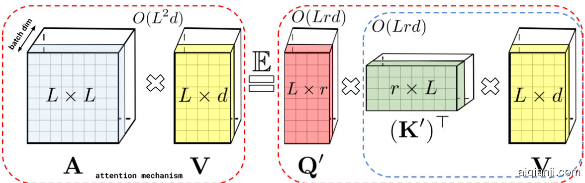
Figure 1: Approximation of the regular attention mechanism AV (before $\mathbf{D}^{-1}$ -re normalization) via (random) feature maps. Dashed-blocks indicate order of computation with corresponding time complexities attached.
图 1: 通过(随机)特征映射对常规注意力机制 AV (在 $\mathbf{D}^{-1}$ 归一化之前)的近似。虚线框表示计算顺序并标注相应时间复杂度。
The above scheme constitutes the FA-part of the $\mathrm{FAVOR+}$ mechanism. The remaining $\mathrm{OR}+$ part answers the following questions: (1) How expressive is the attention model defined in Equation 3, and in particular, can we use it in principle to approximate regular softmax attention ? (2) How do we implement it robustly in practice, and in particular, can we choose $r\ll L$ for $L\gg d$ to obtain desired space and time complexity gains? We answer these questions in the next sections.
上述方案构成了 $\mathrm{FAVOR+}$ 机制的 FA 部分。剩余的 $\mathrm{OR}+$ 部分则解答以下问题:(1) 公式3中定义的注意力模型表达能力如何?特别是,我们能否在原则上用它来近似常规的 softmax 注意力?(2) 如何在实践中稳健地实现它?特别是,对于 $L\gg d$ 的情况,我们能否选择 $r\ll L$ 以获得预期的空间和时间复杂度优势?我们将在接下来的章节中回答这些问题。
2.3 HOW TO AND HOW NOT TO APPROXIMATE SOFTMAX-KERNELS FOR ATTENTION
2.3 如何正确与错误地近似注意力机制中的Softmax核函数
It turns out that by taking $\phi$ of the following form for functions $f_{1},...,f_{l}:\mathbb{R}\to\mathbb{R}$ , function $g:\mathbb{R}^{d}\rightarrow\mathbb{R}$ and deterministic vectors $\omega_{i}$ or $\omega_{1},...,\omega_{m}\overset{\mathrm{iid}}{\sim}\mathcal{D}$ for some distribution $\mathcal{D}\in\mathcal{P}(\mathbb{R}^{d})$ :
结果表明,对于函数 $f_{1},...,f_{l}:\mathbb{R}\to\mathbb{R}$、函数 $g:\mathbb{R}^{d}\rightarrow\mathbb{R}$ 以及确定性向量 $\omega_{i}$ 或从某分布 $\mathcal{D}\in\mathcal{P}(\mathbb{R}^{d})$ 独立同分布抽取的 $\omega_{1},...,\omega_{m}\overset{\mathrm{iid}}{\sim}\mathcal{D}$,采用如下形式的 $\phi$ 时:
$$
\phi(\mathbf{x})=\frac{h(\mathbf{x})}{\sqrt{m}}(f_{1}(\omega_{1}^{\top}\mathbf{x}),...,f_{1}(\omega_{m}^{\top}\mathbf{x}),...,f_{l}(\omega_{1}^{\top}\mathbf{x}),...,f_{l}(\omega_{m}^{\top}\mathbf{x})),
$$
$$
\phi(\mathbf{x})=\frac{h(\mathbf{x})}{\sqrt{m}}(f_{1}(\omega_{1}^{\top}\mathbf{x}),...,f_{1}(\omega_{m}^{\top}\mathbf{x}),...,f_{l}(\omega_{1}^{\top}\mathbf{x}),...,f_{l}(\omega_{m}^{\top}\mathbf{x})),
$$
we can model most kernels used in practice. Furthermore, in most cases $\mathcal{D}$ is isotropic (i.e. with pdf function constant on a sphere), usually Gaussian. For example, by taking $h(\mathbf{x})=1$ , $l=1$ and $\mathbf{\bar{\mathcal{D}}}=\mathcal{N}(0,\mathbf{I}_ {d})$ we obtain estimators of the so-called PNG-kernels (Cho roman ski et al., 2017) (e.g. $f_{1}=\mathrm{sgn}$ corresponds to the angular kernel). Configurations: $h(\mathbf{x})=1$ , $l=2$ , $f_{1}=\sin$ , $f_{2}=\cos$ correspond to shift-invariant kernels, in particular $\mathcal{D}=\mathcal{N}(0,\mathbf{I}_ {d})$ leads to the Gaussian kernel $\mathrm{K_{gauss}}$ (Rahimi & Recht, 2007). The softmax-kernel which defines regular attention matrix $\mathbf{A}$ is given as:
我们可以对实践中使用的大多数核(kernel)进行建模。此外,在大多数情况下$\mathcal{D}$是各向同性的(即概率密度函数在球面上为常数),通常为高斯分布。例如,通过取$h(\mathbf{x})=1$、$l=1$和$\mathbf{\bar{\mathcal{D}}}=\mathcal{N}(0,\mathbf{I}_ {d})$,我们得到了所谓的PNG核(PNG-kernels)估计量(Cho roman ski et al., 2017)(例如$f_{1}=\mathrm{sgn}$对应于角度核(angular kernel))。配置:$h(\mathbf{x})=1$、$l=2$、$f_{1}=\sin$、$f_{2}=\cos$对应于平移不变核(shift-invariant kernels),特别是$\mathcal{D}=\mathcal{N}(0,\mathbf{I}_{d})$会得到高斯核$\mathrm{K_{gauss}}$(Rahimi & Recht, 2007)。定义常规注意力矩阵$\mathbf{A}$的softmax核表示为:
$$
\mathrm{SM}(\mathbf{x},\mathbf{y}){\stackrel{\mathrm{def}}{=}}\exp(\mathbf{x}^{\top}\mathbf{y}).
$$
$$
\mathrm{SM}(\mathbf{x},\mathbf{y}){\stackrel{\mathrm{def}}{=}}\exp(\mathbf{x}^{\top}\mathbf{y}).
$$
In the above, without loss of generality, we omit $\sqrt{d}$ -re normalization since we can equivalently re normalize input keys and queries. Since: $\begin{array}{r}{\mathrm{SM}(\mathbf{x},\mathbf{y})=\exp(\frac{|\mathbf{x}|^{2}}{2})\mathrm{K}_ {\mathrm{gauss}}(\mathbf{x},\mathbf{y})\exp(\frac{|\mathbf{y}|^{2}}{2})}\end{array}$ , based on what we have said, we obtain random feature map unbiased approximation of $\mathrm{SM}(\bar{{\bf x}},{\bf y})$ using trigonometric functions with: $\begin{array}{r}{h(\mathbf{x})=\exp(\frac{|\mathbf{x}|^{2}}{2})}\end{array}$ , $l=2$ , $f_{1}=\sin$ , $f_{2}=\cos$ . We call it $\widehat{\mathrm{SM}}_{m}^{\mathrm{trig}}(\mathbf{x},\mathbf{y})$ There is however a caveat there. The attention module from (1) constructs for each token, a convex combination of value-vectors with coefficients given as corresponding re normalized kernel scores. That is why kernels producing non-negative scores are used. Applying random feature maps with potentially negative dimension-values $(\sin{\it\Delta\phi}/\cos)$ leads to unstable behaviours, especially when kernel scores close to 0 (which is the case for many entries of $\mathbf{A}$ corresponding to low relevance tokens) are approximated by estimators with large variance in such regions. This results in abnormal behaviours, e.g. negative-diagonal-values re normalize rs $\mathbf{D}^{-1}$ , and consequently either completely prevents training or leads to sub-optimal models. We demonstrate empirically that this is what happens for SMm and provide detailed theoretical explanations showing that the variance of SMm is large trig trig asd approximated values tend to 0 (see: Section 3). This is one of the main reasons wdhy the robust random feature map mechanism for approximating regular softmax attention was never proposed.
在上述讨论中,不失一般性,我们省略了 $\sqrt{d}$ 的重新归一化,因为可以等价地对输入键和查询进行重新归一化。由于: $\begin{array}{r}{\mathrm{SM}(\mathbf{x},\mathbf{y})=\exp(\frac{|\mathbf{x}|^{2}}{2})\mathrm{K}_ {\mathrm{gauss}}(\mathbf{x},\mathbf{y})\exp(\frac{|\mathbf{y}|^{2}}{2})}\end{array}$ ,根据前述内容,我们利用三角函数获得了 $\mathrm{SM}(\bar{{\bf x}},{\bf y})$ 的无偏随机特征图近似,其中: $\begin{array}{r}{h(\mathbf{x})=\exp(\frac{|\mathbf{x}|^{2}}{2})}\end{array}$ , $l=2$ , $f_{1}=\sin$ , $f_{2}=\cos$ 。我们称之为 $\widehat{\mathrm{SM}}_{m}^{\mathrm{trig}}(\mathbf{x},\mathbf{y})$ 。
然而这里需要注意一个关键问题。式 (1) 中的注意力模块为每个 token 构建了一个值向量的凸组合,其系数由对应的重新归一化核分数给出。这就是为什么需要使用产生非负分数的核函数。应用可能具有负维度值的随机特征图 $(\sin{\it\Delta\phi}/\cos)$ 会导致不稳定行为,尤其是当接近 0 的核分数(对应于低相关性 token 的 $\mathbf{A}$ 中许多条目)被这些区域方差较大的估计器近似时。这会导致异常行为,例如负对角值的重新归一化矩阵 $\mathbf{D}^{-1}$ ,进而完全阻碍训练或导致次优模型。我们通过实验证明这正是 SMm 出现的问题,并提供详细的理论解释,表明 SMm 的方差在近似值趋近 0 时会显著增大(参见第 3 节)。这也是为什么从未有人提出用于近似常规 softmax 注意力的鲁棒随机特征图机制的主要原因之一。
We propose a robust mechanism in this paper. Furthermore, the variance of our new unbiased positive random feature map estimator tends to 0 as approximated values tend to 0 (see: Section 3).
本文提出了一种鲁棒机制。此外,随着近似值趋近于0,我们新的无偏正随机特征映射估计器的方差也趋近于0(详见:第3节)。
Lemma 1 (Positive Random Features (PRFs) for Softmax). For $\mathbf{x},\mathbf{y}\in\mathbb{R}^{d}$ , ${\bf z}={\bf x}+{\bf y}$ we have:
引理1 (Softmax的正随机特征(PRFs))。对于 $\mathbf{x},\mathbf{y}\in\mathbb{R}^{d}$ , ${\bf z}={\bf x}+{\bf y}$ ,我们有:
$\mathrm{SM}(\mathbf{x},\mathbf{y})=\mathbb{E}_ {\omega\sim\mathcal{N}(0,\mathbf{I}_ {d})}\Big[\mathrm{exp}\Big(\omega^{\top}\mathbf{x}-\frac{|\mathbf{x}|^{2}}{2}\Big)\mathrm{exp}\Big(\omega^{\top}\mathbf{y}-\frac{|\mathbf{y}|^{2}}{2}\Big)\Big]=\Lambda\mathbb{E}_ {\omega\sim\mathcal{N}(0,\mathbf{I}_ {d})}\mathrm{cosh}(\omega^{\top}\mathbf{z}),$ where $\begin{array}{r}{\Lambda=\exp(-\frac{|\mathbf{x}|^{2}+|\mathbf{y}|^{2}}{2})}\end{array}$ and cosh is hyperbolic cosine. Consequently, softmax-kernel admits $a$ positive random feature map unbiased approximation with $\begin{array}{r}{h(\mathbf{x})=\exp(-\frac{\left|\mathbf{x}\right|^{2}}{2})}\end{array}$ , $l=1$ , $f_{1}=\exp$ and $\mathcal{D}=\mathcal{N}(0,\mathbf{I}_ {d})$ or: $\begin{array}{r}{h(\mathbf{x})=\frac{1}{\sqrt{2}}\exp(-\frac{|\mathbf{x}|^{2}}{2})}\end{array}$ , $l=2$ , $f_{1}(u)=\exp(u)$ , $f_{2}(u)=\exp(-u)$ and the same $\mathcal{D}$ (the latter for further variance reduction). We call related estimators: $\widehat{\mathrm{SM}}_ {m}^{+}$ and $\widehat{\mathrm{SM}}_{m}^{\mathrm{hyp+}}$ .
$\mathrm{SM}(\mathbf{x},\mathbf{y})=\mathbb{E}_ {\omega\sim\mathcal{N}(0,\mathbf{I}_ {d})}\Big[\mathrm{exp}\Big(\omega^{\top}\mathbf{x}-\frac{|\mathbf{x}|^{2}}{2}\Big)\mathrm{exp}\Big(\omega^{\top}\mathbf{y}-\frac{|\mathbf{y}|^{2}}{2}\Big)\Big]=\Lambda\mathbb{E}_ {\omega\sim\mathcal{N}(0,\mathbf{I}_ {d})}\mathrm{cosh}(\omega^{\top}\mathbf{z}),$ 其中 $\begin{array}{r}{\Lambda=\exp(-\frac{|\mathbf{x}|^{2}+|\mathbf{y}|^{2}}{2})}\end{array}$ 且 cosh 为双曲余弦函数。因此,softmax核函数允许通过正随机特征映射进行无偏近似,其中 $\begin{array}{r}{h(\mathbf{x})=\exp(-\frac{\left|\mathbf{x}\right|^{2}}{2})}\end{array}$,$l=1$,$f_{1}=\exp$ 且 $\mathcal{D}=\mathcal{N}(0,\mathbf{I}_ {d})$;或采用 $\begin{array}{r}{h(\mathbf{x})=\frac{1}{\sqrt{2}}\exp(-\frac{|\mathbf{x}|^{2}}{2})}\end{array}$,$l=2$,$f_{1}(u)=\exp(u)$,$f_{2}(u)=\exp(-u)$ 及相同 $\mathcal{D}$(后者可进一步降低方差)。我们将相关估计器称为:$\widehat{\mathrm{SM}}_ {m}^{+}$ 和 $\widehat{\mathrm{SM}}_{m}^{\mathrm{hyp+}}$。

Figure 2: Left: Sym met rize d (around origin) utility function $r$ (defined as the ratio of the mean squared errors (MSEs) of estimators built on: trigonometric and positive random features) as a function of the angle $\phi$ (in radians) between input feature vectors and their lengths $l$ . Larger values indicate regions of $(\phi,l)$ -space with better performance of positive random features. We see that for critical regions with $\phi$ large enough (small enough softmax-kernel values) our method is arbitrarily more accurate than trigonometric random features. Plot presented for domain $[-\pi,\pi]\times[-2,2]$ . Right: The slice of function $r$ for fixed $l=1$ and varying angle $\phi$ . Right Upper Corner: Comparison of the MSEs of both the estimators in a low softmax-kernel value region.
图 2: 左图: 对称化(关于原点)的效用函数 $r$ (定义为基于三角随机特征和正随机特征构建的估计器均方误差(MSE)之比)随输入特征向量间夹角 $\phi$ (弧度制)及其长度 $l$ 变化的关系。较大值表示 $(\phi,l)$ 空间中正随机特征性能更优的区域。可见在 $\phi$ 足够大(softmax核函数值足够小)的关键区域,我们的方法比三角随机特征精度有显著提升。绘图展示区间为 $[-\pi,\pi]\times[-2,2]$。右图: 固定 $l=1$ 时函数 $r$ 随角度 $\phi$ 变化的切片。右上角: 在softmax核函数值较低区域两种估计器MSE的对比。
In Fig. 2 we visualize the advantages of positive versus standard trigonometric random features. In critical regions, where kernel values are small and need careful approximation, our method outperforms its counterpart. In Section 4 we further confirm our method’s advantages empirically, using positive features to efficiently train softmax-based linear Transformers. If we replace in (7) $\omega$ with $\sqrt{d}\frac{\omega}{|\omega|}$ , we obtain the so-called regularized softmax-kernel SMREG which we can approximate in a similar manner, simply changing $\mathcal{D}=\mathcal{N}(0,\mathbf{I}_ {d})$ to ${\mathcal{D}}={\mathrm{Unif}}({\sqrt{d}}S^{d-1})$ , a distribution corresponding to Haar measure on the sphere of radius $\sqrt{d}$ in $\mathbb{R}^{d}$ , obtaining estimator $\widehat{\mathrm{SMREG}_{m}^{+}}$ . As we show in Section 3, such random features can also be used to accurately approximate regular softmax-kernel.
在图 2 中,我们展示了正三角随机特征相对于标准三角随机特征的优势。在核值较小且需要精确逼近的关键区域,我们的方法表现优于对比方案。在第 4 节中,我们通过实验进一步验证了该方法的优势,使用正特征高效训练基于 softmax 的线性 Transformer。若将式 (7) 中的 $\omega$ 替换为 $\sqrt{d}\frac{\omega}{|\omega|}$ ,则可得到所谓的正则化 softmax 核 SMREG,我们可用类似方式进行逼近,只需将 $\mathcal{D}=\mathcal{N}(0,\mathbf{I}_ {d})$ 改为 ${\mathcal{D}}={\mathrm{Unif}}({\sqrt{d}}S^{d-1})$ (该分布对应于 $\mathbb{R}^{d}$ 中半径为 $\sqrt{d}$ 的球面上的哈尔测度),从而获得估计量 $\widehat{\mathrm{SMREG}_{m}^{+}}$ 。如第 3 节所示,此类随机特征也可用于精确逼近常规 softmax 核。
2.4 ORTHOGONAL RANDOM FEATURES (ORFS)
2.4 正交随机特征 (ORFs)
The above constitutes the $\mathsf{R}+$ part of the $\mathrm{FAVOR+}$ method. It remains to explain the O-part. To further reduce the variance of the estimator (so that we can use an even smaller number of random features $r$ ), we entangle different random samples $\omega_{1},...,\omega_{m}$ to be exactly orthogonal. This can be done while maintaining unbiased ness whenever isotropic distributions $\mathcal{D}$ are used (i.e. in particular in all kernels we considered so far) by the standard Gram-Schmidt orthogonal iz ation procedure (see (Cho roman ski et al., 2017) for details). ORFs is a well-known method, yet it turns out that it works particularly well with our introduced PRFs for softmax. This leads to the first theoretical results showing that ORFs can be applied to reduce the variance of softmax/Gaussian kernel estimators for any dimensionality $d$ rather than just asymptotically for large enough $d$ (as is the case for previous methods, see: next section) and leads to the first exponentially small bounds on large deviations probabilities that are strictly smaller than for non-orthogonal methods. Positivity of random features plays a key role in these bounds. The ORF mechanism requires $m\leq d$ , but this will be the case in all our experiments. The pseudocode of the entire $\mathrm{FAVOR+}$ algorithm is given in Appendix B.
上述内容构成了 $\mathrm{FAVOR+}$ 方法的 $\mathsf{R}+$ 部分。接下来需要解释O部分。为了进一步降低估计器的方差(从而可以使用更少的随机特征 $r$),我们将不同的随机样本 $\omega_{1},...,\omega_{m}$ 进行正交化处理。在使用各向同性分布 $\mathcal{D}$ 时(即特别是目前为止我们考虑的所有核函数),通过标准的Gram-Schmidt正交化程序(详见 (Cho roman ski et al., 2017)),可以在保持无偏性的同时实现这一点。ORFs是一种众所周知的方法,但事实证明它特别适用于我们提出的softmax PRFs。这首次从理论上证明,ORFs可以应用于降低任何维度 $d$ 下softmax/高斯核估计器的方差,而不仅仅是在足够大的 $d$ 时渐进有效(如之前的方法所示,见下一节),并且首次得到了严格小于非正交方法的指数级小的大偏差概率界。随机特征的正定性在这些界中起着关键作用。ORF机制要求 $m\leq d$,但这在我们所有的实验中都会满足。完整的 $\mathrm{FAVOR+}$ 算法伪代码见附录B。
Our theoretical results are tightly aligned with experiments. We show in Section 4 that PRFs $^{+}$ ORFs drastically improve accuracy of the approximation of the attention matrix and enable us to reduce $r$ which results in an accurate as well as space and time efficient mechanism which we call FAVOR+.
我们的理论结果与实验高度吻合。在第4节中,我们将展示PRFs$^{+}$ORFs能显著提升注意力矩阵近似的准确度,并使我们能够减小$r$,从而获得一种既精确又节省空间和时间的机制,我们称之为FAVOR+。
3 THEORETICAL RESULTS
3 理论结果
We present here the theory of positive orthogonal random features for softmax-kernel estimation. All these results can be applied also to the Gaussian kernel, since as explained in the previous section, one can be obtained from the other by re normalization (see: Section 2.3). All proofs and additional more general theoretical results with a discussion are given in the Appendix.
我们在此提出用于softmax核估计的正交随机特征理论。所有这些结果同样适用于高斯核 (Gaussian kernel) ,因为正如前文所述,通过重新归一化可以从一个核获得另一个核 (参见:第2.3节) 。所有证明及更一般的理论结果与讨论详见附录。
Lemma 2 (positive (hyperbolic) versus trigonometric random features). The following is true:
引理 2 (正(双曲)与三角随机特征). 以下结论成立:
$$
\begin{array}{r l r}&{}&{\mathrm{MSE}(\widehat{\mathrm{SM}}_ {m}^{\mathrm{trig}}({\bf x},{\bf y}))=\displaystyle\frac{1}{2m}\exp(|{\bf x}+{\bf y}|^{2})\mathrm{SM}^{-2}({\bf x},{\bf y})(1-\exp(-|{\bf x}-{\bf y}|^{2}))^{2},}\ &{}&{\mathrm{MSE}(\widehat{\mathrm{SM}}_ {m}^{+}({\bf x},{\bf y}))=\displaystyle\frac{1}{m}\exp(|{\bf x}+{\bf y}|^{2})\mathrm{SM}^{2}({\bf x},{\bf y})(1-\exp(-|{\bf x}+{\bf y}|^{2})),}\ &{}&{\mathrm{MSE}(\widehat{\mathrm{SM}}_ {m}^{\mathrm{byp}+}({\bf x},{\bf y}))=\displaystyle\frac{1}{2}(1-\exp(-|{\bf x}+{\bf y}|^{2}))\mathrm{MSE}(\widehat{\mathrm{SM}}_{m}^{+}({\bf x},{\bf y})),}\end{array}
$$
$$
\begin{array}{r l r}&{}&{\mathrm{MSE}(\widehat{\mathrm{SM}}_ {m}^{\mathrm{trig}}({\bf x},{\bf y}))=\displaystyle\frac{1}{2m}\exp(|{\bf x}+{\bf y}|^{2})\mathrm{SM}^{-2}({\bf x},{\bf y})(1-\exp(-|{\bf x}-{\bf y}|^{2}))^{2},}\ &{}&{\mathrm{MSE}(\widehat{\mathrm{SM}}_ {m}^{+}({\bf x},{\bf y}))=\displaystyle\frac{1}{m}\exp(|{\bf x}+{\bf y}|^{2})\mathrm{SM}^{2}({\bf x},{\bf y})(1-\exp(-|{\bf x}+{\bf y}|^{2})),}\ &{}&{\mathrm{MSE}(\widehat{\mathrm{SM}}_ {m}^{\mathrm{byp}+}({\bf x},{\bf y}))=\displaystyle\frac{1}{2}(1-\exp(-|{\bf x}+{\bf y}|^{2}))\mathrm{MSE}(\widehat{\mathrm{SM}}_{m}^{+}({\bf x},{\bf y})),}\end{array}
$$
for independent random samples $\omega_{i}$ , and where MSE stands for the mean squared error.
对于独立随机样本 $\omega_{i}$,其中 MSE 表示均方误差。
Thus, for $\mathrm{SM}(\mathbf{x},\mathbf{y})\rightarrow0$ we have: $\mathrm{MSE}(\widehat{\mathrm{SM}}_ {m}^{\mathrm{trig}}({\bf x},{\bf y}))\rightarrow\infty$ and $\mathrm{MSE}(\widehat{\mathrm{SM}}_ {m}^{+}({\bf x},{\bf y}))\rightarrow0$ . Furthermore, the hyperbolic estimator provides a ddd it ional accuracy improve med nts that are strictly better than those from $\widehat{\mathrm{SM}}_{2m}^{+}(\mathbf{x},\mathbf{y})$ with twice as many random features. The next result shows that the regularized soft madx-kernel is in practice an accurate proxy of the softmax-kernel in attention.
因此,当 $\mathrm{SM}(\mathbf{x},\mathbf{y})\rightarrow0$ 时,我们有:$\mathrm{MSE}(\widehat{\mathrm{SM}}_ {m}^{\mathrm{trig}}({\bf x},{\bf y}))\rightarrow\infty$ 且 $\mathrm{MSE}(\widehat{\mathrm{SM}}_ {m}^{+}({\bf x},{\bf y}))\rightarrow0$。此外,双曲估计器提供了额外的精度提升,其表现严格优于使用两倍随机特征的 $\widehat{\mathrm{SM}}_{2m}^{+}(\mathbf{x},\mathbf{y})$。接下来的结果表明,正则化后的softmax核实际上是注意力机制中softmax核的精确代理。
Theorem 1 (regularized versus softmax-kernel). Assume that the $L_{\infty}$ -norm of the attention matrix for the softmax-kernel satisfies: $|\mathbf{A}|_{\infty}\leq C$ for some constant $C~\geq~1$ . Denote by $\mathbf{A}^{\mathrm{reg}}$ the corresponding attention matrix for the regularized softmax-kernel. The following holds:
定理1 (正则化与softmax核). 假设softmax核的注意力矩阵满足 $L_{\infty}$ 范数条件: $|\mathbf{A}|_{\infty}\leq C$ (其中常数 $C~\geq~1$). 记 $\mathbf{A}^{\mathrm{reg}}$ 为正则化softmax核对应的注意力矩阵, 则有:
$$
\operatorname*{inf}_ {i,j}\frac{\mathbf{A}^{\mathrm{reg}}(i,j)}{\mathbf{A}(i,j)}\geq1-\frac{2}{d^{\frac{1}{3}}}+o\left(\frac{1}{d^{\frac{1}{3}}}\right),a n d\operatorname*{sup}_{i,j}\frac{\mathbf{A}^{\mathrm{reg}}(i,j)}{\mathbf{A}(i,j)}\leq1.
$$
$$
\operatorname*{inf}_ {i,j}\frac{\mathbf{A}^{\mathrm{reg}}(i,j)}{\mathbf{A}(i,j)}\geq1-\frac{2}{d^{\frac{1}{3}}}+o\left(\frac{1}{d^{\frac{1}{3}}}\right),a n d\operatorname*{sup}_{i,j}\frac{\mathbf{A}^{\mathrm{reg}}(i,j)}{\mathbf{A}(i,j)}\leq1.
$$
Furthermore, the latter holds for $d\geq2$ even if the $L_{\infty}$ -norm condition is not satisfied, i.e. the regularized softmax-kernel is a universal lower bound for the softmax-kernel.
此外,即使不满足 $L_{\infty}$ 范数条件,后者在 $d\geq2$ 时仍然成立,即正则化 softmax-kernel 是 softmax-kernel 的通用下界。
Consequently, positive random features for SMREG can be used to approximate the softmax-kernel. Our next result shows that orthogonality provably reduces mean squared error of the estimation with positive random features for any dimensionality $d>0$ and we explicitly provide the gap.
因此,SMREG的正随机特征可用于近似softmax核函数。我们的下一个结果表明,对于任意维度$d>0$,正交性可证明降低正随机特征估计的均方误差,并明确给出了误差差距。
Theorem 2. If $\widehat{\mathrm{SM}}_ {m}^{\mathrm{ort+}}(\mathbf{x},\mathbf{y})$ stands for the modification of $\widehat{\mathrm{SM}}_{m}^{+}(\mathbf{x},\mathbf{y})$ with orthogonal random features (and th usd for $m\leq d,$ ), then the following holds for an y $d>0$ :
定理 2. 若 $\widehat{\mathrm{SM}}_ {m}^{\mathrm{ort+}}(\mathbf{x},\mathbf{y})$ 表示采用正交随机特征改进后的 $\widehat{\mathrm{SM}}_{m}^{+}(\mathbf{x},\mathbf{y})$ (因此适用于 $m\leq d$ ), 则对于任意 $d>0$ 有:
$$
\mathrm{dSE}(\widehat{\mathrm{SM}}_ {m}^{\mathrm{ort+}}(\mathbf{x},\mathbf{y}))\leq\mathrm{MSE}(\widehat{\mathrm{SM}}_{m}^{+}(\mathbf{x},\mathbf{y}))-\frac{2(m-1)}{m(d+2)}\left(\mathrm{SM}(\mathbf{x},\mathbf{y})-\exp\left(-\frac{|\mathbf{x}|^{2}+|\mathbf{y}|^{2}}{2}\right)\right)^{2}.
$$
$$
\mathrm{dSE}(\widehat{\mathrm{SM}}_ {m}^{\mathrm{ort+}}(\mathbf{x},\mathbf{y}))\leq\mathrm{MSE}(\widehat{\mathrm{SM}}_{m}^{+}(\mathbf{x},\mathbf{y}))-\frac{2(m-1)}{m(d+2)}\left(\mathrm{SM}(\mathbf{x},\mathbf{y})-\exp\left(-\frac{|\mathbf{x}|^{2}+|\mathbf{y}|^{2}}{2}\right)\right)^{2}.
$$
Furthermore, completely analogous result holds for the regularized softmax-kernel SMREG.
此外,完全类似的结果也适用于正则化 softmax 核 (SMREG)。
For the regularized softmax-kernel, orthogonal features provide additional concentration results - the first exponentially small bounds for probabilities of estimators’ tails that are strictly better than for non-orthogonal variants for every $d>0$ . Our next result enables us to explicitly estimate the gap.
对于正则化的 softmax 核函数,正交特征提供了额外的集中性结果——这是首个关于估计量尾概率的指数级小界,且对于所有 $d>0$ 都严格优于非正交变体。我们的下一个结果使我们能够明确估计这一差距。
Theorem 3. Let x $\cdot,\mathbf{y}\in\mathbb{R}^{d}$ . The following holds for any $a>\mathrm{SMREG}(\mathbf{x},\mathbf{y})$ , $\theta>0$ and $m\leq d$ :
定理3. 设x $\cdot,\mathbf{y}\in\mathbb{R}^{d}$。对于任意$a>\mathrm{SMREG}(\mathbf{x},\mathbf{y})$、$\theta>0$和$m\leq d$,以下不等式成立:
$$
\begin{array}{r l}&{\widehat{\mathbb{P}[\widehat{\mathrm{SMREG}}_ {m}^{+}(\mathbf{x},\mathbf{y})>a]}\le\exp(-\theta m a)M_{Z}(\theta)^{m},\quad\widehat{\mathbb{P}[\widehat{\mathrm{SMREG}}_ {m}^{\mathrm{ort+}}(\mathbf{x},\mathbf{y})>a]}}\ &{\le\exp(-\theta m a)\bigg(M_{Z}(\theta)^{m}-\exp\left(-\frac{m}{2}(|\mathbf{x}|^{2}+|\mathbf{y}|^{2})\right)\frac{\theta^{4}m(m-1)}{4(d+2)}|\mathbf{x}+\mathbf{y}|^{4}\bigg)}\end{array}
$$
$$
\begin{array}{r l}&{\widehat{\mathbb{P}[\widehat{\mathrm{SMREG}}_ {m}^{+}(\mathbf{x},\mathbf{y})>a]}\le\exp(-\theta m a)M_{Z}(\theta)^{m},\quad\widehat{\mathbb{P}[\widehat{\mathrm{SMREG}}_ {m}^{\mathrm{ort+}}(\mathbf{x},\mathbf{y})>a]}}\ &{\le\exp(-\theta m a)\bigg(M_{Z}(\theta)^{m}-\exp\left(-\frac{m}{2}(|\mathbf{x}|^{2}+|\mathbf{y}|^{2})\right)\frac{\theta^{4}m(m-1)}{4(d+2)}|\mathbf{x}+\mathbf{y}|^{4}\bigg)}\end{array}
$$
where $\widehat{\mathrm{SMREG}}_ {m}^{\mathrm{ort+}}(\mathbf{x},\mathbf{y})$ stands for the modification of $\widehat{\mathrm{SMREG}_ {m}^{+}(\mathbf{x},\mathbf{y})}$ with ORFs, $\boldsymbol{X}=$ $\begin{array}{r}{\Lambda\exp(\sqrt{d}\frac{\omega^{\top}}{|\omega|_ {2}}({\bf x}+{\bf y}))}\end{array}$ , $\omega\sim\mathcal{N}(0,\mathbf{I}_ {d})$ , $\Lambda$ is as in Lemma $I$ and $M_{Z}$ is the moment generating function of $Z$ .
其中 $\widehat{\mathrm{SMREG}}_ {m}^{\mathrm{ort+}}(\mathbf{x},\mathbf{y})$ 表示用 ORFs 改进的 $\widehat{\mathrm{SMREG}_ {m}^{+}(\mathbf{x},\mathbf{y})}$,$\boldsymbol{X}=$ $\begin{array}{r}{\Lambda\exp(\sqrt{d}\frac{\omega^{\top}}{|\omega|_ {2}}({\bf x}+{\bf y}))}\end{array}$,$\omega\sim\mathcal{N}(0,\mathbf{I}_ {d})$,$\Lambda$ 如引理 $I$ 所述,$M_{Z}$ 是 $Z$ 的矩母函数。
We see that ORFs provide exponentially small and sharper bounds for critical regions where the softmax-kernel is small. Below we show that even for the $\mathrm{SM}^{\mathrm{trig}}$ mechanism with ORFs, it suffices to take $m=\Theta(d\log(d))$ random projections to accurately approximate the attention matrix (thus if not attention re normalization, PRFs would not be needed). In general, $m$ depends on the dimensionality $d$ of the embeddings, radius $R$ of the ball where all queries/keys live and precision parameter $\epsilon$ (see: Appendix F.6 for additional discussion), but does not depend on input sequence length $L$ .
我们发现,ORFs(正交随机特征)为softmax核函数较小的关键区域提供了指数级更小且更尖锐的边界。下文将证明,即使对于采用ORFs的$\mathrm{SM}^{\mathrm{trig}}$机制,也只需$m=\Theta(d\log(d))$次随机投影即可精确逼近注意力矩阵(因此若非注意力重归一化,PRFs将不再必需)。一般而言,$m$取决于嵌入维度$d$、所有查询/键所在球的半径$R$以及精度参数$\epsilon$(详见附录F.6的进一步讨论),但与输入序列长度$L$无关。
Theorem 4 (uniform convergence for attention approximation). Assume that $L_{2}$ -norms of queries/keys are upper-bounded by $R>0$ . Define $l~=~R d^{-\frac{1}{4}}$ and take $\begin{array}{r}{h^{\ast}=\exp(\frac{l^{2}}{2})}\end{array}$ . Then for any $\epsilon>0$ , $\begin{array}{r}{\delta=\frac{\epsilon}{(h^{*})^{2}}}\end{array}$ and the number of random projections $\begin{array}{r}{m=\Theta(\frac{d}{\delta^{2}}\log(\frac{4d^{\frac{3}{4}}R}{\delta}))}\end{array}$ the following holds for the attention approximation mechanism leveraging estimators $\widehat{\mathrm{SM}}^{\mathrm{trig}}$ with ORFs: $|\widehat{\mathbf A}-\mathbf A|_{\infty}\le\epsilon$ with any constant probability, where $\widehat{\bf A}$ approximates the attent iodn matrix A.
定理4 (注意力近似的一致收敛性)。假设查询/键的$L_{2}$-范数上界为$R>0$。定义$l~=~R d^{-\frac{1}{4}}$并取$\begin{array}{r}{h^{\ast}=\exp(\frac{l^{2}}{2})}\end{array}$。则对于任意$\epsilon>0$,$\begin{array}{r}{\delta=\frac{\epsilon}{(h^{*})^{2}}}\end{array}$和随机投影数量$\begin{array}{r}{m=\Theta(\frac{d}{\delta^{2}}\log(\frac{4d^{\frac{3}{4}}R}{\delta}))}\end{array}$,以下结论对采用ORF估计器$\widehat{\mathrm{SM}}^{\mathrm{trig}}$的注意力近似机制成立:以任意常数概率有$|\widehat{\mathbf A}-\mathbf A|_{\infty}\le\epsilon$,其中$\widehat{\bf A}$是注意力矩阵A的近似。
4 EXPERIMENTS
4 实验
We implemented our setup on top of pre-existing Transformer training code in Jax (Frostig et al., 2018) optimized with just-in-time $(\ j a x\cdot\ j\mathtt{i t})$ compilation, and complement our theory with empirical evidence to demonstrate the practicality of $\mathrm{FAVOR+}$ in multiple settings. Unless explicitly stated, a Performer replaces only the attention component with our method, while all other components are exactly the same as for the regular Transformer. For shorthand notation, we denote unidirectional/causal modelling as (U) and bidirectional/masked language modelling as (B).
我们在Jax (Frostig等人,2018) 现有的Transformer训练代码基础上实现了实验配置,通过即时编译 $(jax \cdot jit)$ 进行优化,并用实证数据补充理论分析,以证明FAVOR+在多种场景下的实用性。除非特别说明,Performer仅用我们的方法替换注意力模块,其余组件与常规Transformer完全相同。简写标记中,单向/因果建模记为(U),双向/掩码语言建模记为(B)。
In terms of baselines, we use other Transformer models for comparison, although some of them are restricted to only one case - e.g. Reformer (Kitaev et al., 2020) is only (U), and Linformer (Wang et al., 2020) is only (B). Furthermore, we use PG-19 (Rae et al., 2020) as an alternative (B) pre training benchmark, as it is made for long-length sequence training compared to the (now publicly unavailable) BookCorpus (Zhu et al., 2015) $^+$ Wikipedia dataset used in BERT (Devlin et al., 2018) and Linformer. All model and token iz ation hyper parameters are shown in Appendix A.
在基线方面,我们使用其他Transformer模型进行比较,尽管其中一些仅限于单一场景——例如Reformer (Kitaev et al., 2020)仅支持(U)情况,Linformer (Wang et al., 2020)仅支持(B)情况。此外,我们采用PG-19 (Rae et al., 2020)作为替代的(B)预训练基准,因为相比BERT (Devlin et al., 2018)和Linformer使用的(现已公开不可用的)BookCorpus (Zhu et al., 2015) $^+$ Wikipedia数据集,PG-19专为长序列训练设计。所有模型和token化的超参数详见附录A。
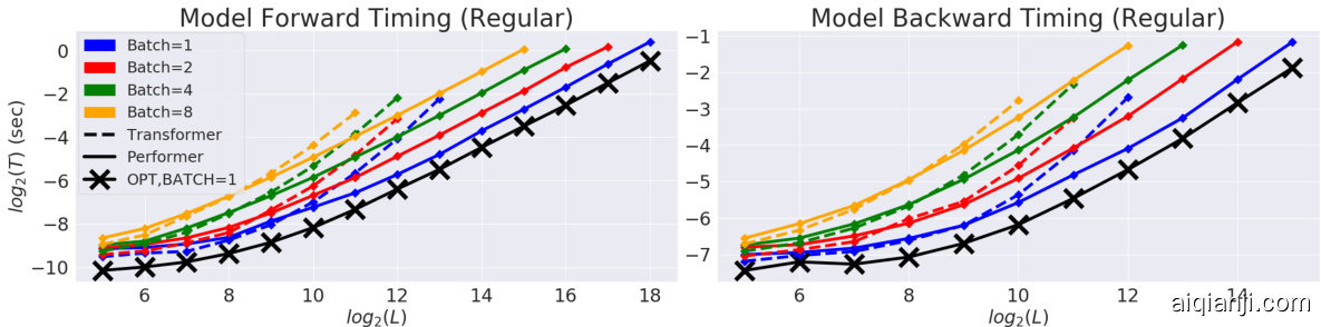
Figure 3: Comparison of Transformer and Performer in terms of forward and backward pass speed and maximum $L$ allowed. "X" (OPT) denotes the maximum possible speedup achievable, when attention simply returns the $\mathbf{V}$ -matrix. Plots shown up to when a model produces an out of memory error on a V100 GPU with 16GB. Vocabulary size used was 256. Best in color.
图 3: Transformer 和 Performer 在前向传播与反向传播速度及最大允许序列长度 $L$ 上的对比。 "X" (OPT) 表示注意力机制直接返回 $\mathbf{V}$ 矩阵时可达到的理论最大加速比。实验在显存为16GB的V100 GPU上进行,当模型触发内存错误时停止测试。词表大小设置为256。建议查看彩色版本。
4.1 COMPUTATIONAL COSTS
4.1 计算成本
We compared speed-wise the backward pass of the Transformer and the Performer in (B) setting, as it is one of the main computational bottlenecks during training, when using the regular default size $(n_{h e a d s},n_{l a y e r s},d_{f f},d\bar{)}=(8,6,2048,512)$ , where $d_{f f}$ denotes the width of the MLP layers.
我们在(B)设置下比较了Transformer和Performer的反向传播速度,因为这是训练过程中的主要计算瓶颈之一。测试使用的是常规默认尺寸$(n_{heads},n_{layers},d_{ff},d\bar{)}=(8,6,2048,512)$,其中$d_{ff}$表示MLP层的宽度。
We observed (Fig. 3) that in terms of $L$ , the Performer reaches nearly linear time and sub-quadratic memory consumption (since the explicit $O(L^{2})$ attention matrix is not stored). In fact, the Performer achieves nearly optimal speedup and memory efficiency possible, depicted by the "X"-line when attention is replaced with the "identity function" simply returning the $\mathbf{V}$ -matrix. The combination of both memory and backward pass efficiencies for large $L$ allows respectively, large batch training and lower wall clock time per gradient step. Extensive additional results are demonstrated in Appendix E by varying layers, raw attention, and architecture sizes.
我们观察到 (图 3) ,在 $L$ 方面,Performer 达到了近乎线性的时间和次二次方的内存消耗 (因为显式的 $O(L^{2})$ 注意力矩阵未被存储) 。实际上,Performer 实现了近乎最优的速度提升和内存效率,如用返回 $\mathbf{V}$ 矩阵的"恒等函数"替代注意力时的"X"线所示。对于大 $L$ ,内存和后向传播效率的结合分别支持了大批量训练和更短的每梯度步实际耗时。附录 E 通过变化层数、原始注意力和架构规模展示了更多实验结果。
4.2 SOFTMAX ATTENTION APPROXIMATION ERROR
4.2 SOFTMAX注意力近似误差
We further examined the approximation error via $\mathrm{FAVOR+}$ in Fig. 4. We demonstrate that 1. Orthogonal features produce lower error than unstructured (IID) features, 2. Positive features produce lower error than trigonometric sin/cos features. These two empirically validate the PORF mechanism.
我们进一步通过图4中的$\mathrm{FAVOR+}$检验了近似误差。结果表明:1. 正交特征比非结构化(IID)特征产生更低的误差;2. 正特征比三角函数sin/cos特征产生更低的误差。这两点从实证角度验证了PORF机制。
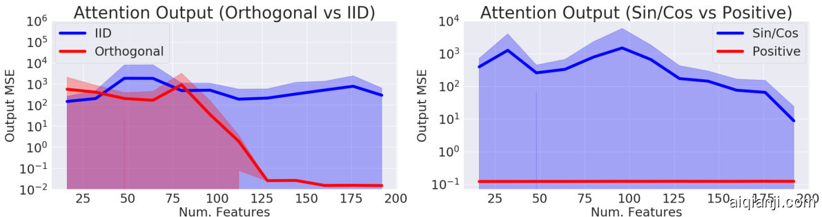
Figure 4: MSE of the approximation output when comparing Orthogonal vs IID features and trigonometric sin/cos vs positive features. We took $L=4096$ , $d=16$ , and varied the number of random samples $m$ . Standard deviations shown across 15 samples of appropriately normalized random matrix input data.
图 4: 正交特征与独立同分布(IID)特征、三角函数sin/cos与正特征在近似输出时的均方误差(MSE)对比。实验参数设置为$L=4096$、$d=16$,并随机采样数量$m$进行变量控制。误差线表示对15组经过适当归一化的随机矩阵输入数据的标准差。
To further improve overall approximation of attention blocks across multiple iterations which further improves training, random samples should be periodically redrawn (Fig. 5, right). This is a cheap procedure, but can be further optimized (Appendix B.2).
为了进一步提升多轮迭代中注意力块的整体近似效果(从而改善训练效果),应定期重新抽取随机样本(图 5,右)。这一过程计算成本较低,但可进一步优化(附录 B.2)。
4.3 SOFTMAX APPROXIMATION ON TRANSFORMERS
4.3 Transformer 上的 Softmax 近似
Even if the approximation of the attention mechanism is tight, small errors can easily propagate throughout multiple Transformer layers (e.g. MLPs, multiple heads), as we show in Fig. 14 (Appendix). In other words, the model’s Lipschitz constant can easily scale up small attention approximation error, which means that very tight approximations may sometimes be needed. Thus, when applying $\operatorname{FAVOR}(+)$ ’s softmax approximations on a Transformer model (i.e. "Performer-XSOFTMAX"), we demonstrate that:
即使注意力机制的近似足够紧密,微小的误差仍容易在多个Transformer层(如MLP、多头注意力)中传播,如图14(附录)所示。换言之,模型的Lipschitz常数容易放大注意力近似误差,这意味着有时需要极其精确的近似。因此,在Transformer模型上应用$\operatorname{FAVOR}(+)$的softmax近似(即"Performer-XSOFTMAX")时,我们证明:
- Backwards compatibility with pretrained models is available as a benefit from softmax approximation, via small finetuning (required due to error propagation) even for trigonometric features (Fig. 5, left) on the LM1B dataset (Chelba et al., 2014). However, when on larger dataset PG-19, 2. Positive (POS) softmax features (with redrawing) become crucial for achieving performance matching regular Transformers (Fig. 5, right).
- 通过softmax近似带来的优势,可实现与预训练模型的向后兼容性,即使在LM1B数据集 (Chelba et al., 2014) 上针对三角特征 (图5左) 也只需少量微调 (由于误差传播而必需) 。然而在更大规模的PG-19数据集上
- 正向 (POS) softmax特征 (带重绘) 成为实现与常规Transformer性能匹配的关键要素 (图5右)
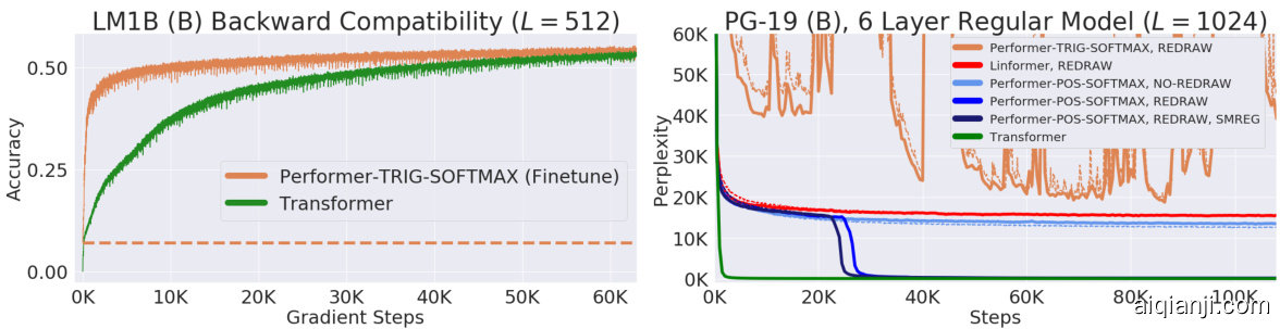
Figure 5: We transferred the original pretrained Transformer’s weights into the Performer, which produces an initial non-zero 0.07 accuracy (dotted orange line), but quickly recovers accuracy in a small fraction of the original number of gradient steps. However on PG-19, Trigonometric (TRIG) softmax approximation becomes highly unstable (full curve in Appendix D.2), while positive features (POS) (without redrawing) and Linformer (which also approximates softmax) even with redrawn projections, plateau at the same perplexity. Positive softmax with feature redrawing is necessary to match the Transformer, with SMREG (regular iz ation from Sec. 3) allowing faster convergence. Additional ablation studies over many attention kernels, showing also that trigonometric random features lead even to NaN values in training are given in Appendix D.3.
图 5: 我们将原始预训练 Transformer 的权重迁移到 Performer 中,初始获得了非零的 0.07 准确率 (橙色虚线),但在原始梯度步数的一小部分内迅速恢复了准确率。然而在 PG-19 数据集上,三角 (TRIG) softmax 近似变得极不稳定 (完整曲线见附录 D.2),而正特征 (POS) (无需重绘) 和 Linformer (同样近似 softmax) 即使采用重绘投影,困惑度仍停滞在同一水平。只有采用特征重绘的正 softmax 才能匹配 Transformer 表现,配合 SMREG (第 3 节的正则化方法) 可实现更快收敛。附录 D.3 提供了对多种注意力核的消融研究,表明三角随机特征甚至会导致训练中出现 NaN 值。
4.4 MULTIPLE LAYER TRAINING FOR PROTEINS
4.4 蛋白质的多层训练
We further benchmark the Performer on both (U) and (B) cases by training a 36-layer model using protein sequences from the Jan. 2019 release of TrEMBL (Consortium, 2019), similar to (Madani et al., 2020). In Fig. 6, the Reformer and Linformer significantly drop in accuracy on the protein dataset. Furthermore, the usefulness of generalized attention is evidenced by Performer-RELU (taking $f=\mathrm{ReLU}$ in Equation 5) achieving the highest accuracy in both (U) and (B) cases. Our proposed softmax approximation is also shown to be tight, achieving the same accuracy as the exact-softmax Transformer and confirming our theoretical claims from Section 3.
我们进一步在(U)和(B)两种情况下对Performer进行基准测试,使用2019年1月发布的TrEMBL蛋白质序列(Consortium, 2019)训练了一个36层模型,方法类似于(Madani et al., 2020)。在图6中,Reformer和Linformer在蛋白质数据集上的准确率显著下降。此外,广义注意力机制的有效性通过Performer-RELU(在公式5中取$f=\mathrm{ReLU}$)在(U)和(B)情况下均获得最高准确率得到证实。我们提出的softmax近似也被证明是紧致的,达到了与精确softmax Transformer相同的准确率,验证了第3节的理论主张。
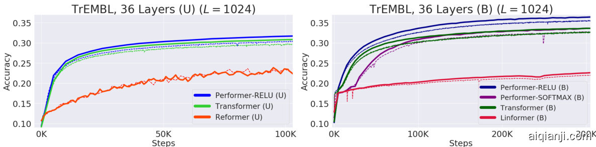
Figure 6: Train $=$ Dashed, Validation $=$ Solid. For TrEMBL, we used the exact same model parameters $(n_{h e a d s},n_{l a y e r s},d_{f f},d)=(8,36,1024,512)$ from (Madani et al., 2020) for all runs. For fairness, all TrEMBL experiments used 16x16 TPU-v2’s. Batch sizes were maximized for each separate run given the compute constraints. Hyper parameters can be found in Appendix A. Extended results including dataset statistics, out of distribution evaluations, and visualization s, can be found in Appendix C.
图 6: 训练集 $=$ 虚线, 验证集 $=$ 实线。对于TrEMBL, 我们在所有实验中均采用与 (Madani et al., 2020) 完全相同的模型参数 $(n_{heads},n_{layers},d_{ff},d)=(8,36,1024,512)$。为确保公平性, 所有TrEMBL实验均使用16x16 TPU-v2芯片。在计算资源限制下, 每次实验的批次大小均设置为最大值。超参数详见附录A。扩展结果 (包括数据集统计、分布外评估和可视化) 详见附录C。
4.5 LARGE LENGTH TRAINING - COMMON DATASETS
4.5 大长度训练 - 常用数据集
On the standard (U) ImageNet64 benchmark from (Parmar et al., 2018) with $L=12288$ which is unfeasible for regular Transformers, we set all models to use the same $(n_{h e a d s},d_{f f},d)$ but varying $\it{n_{l a y e r s}}$ . Performer/6-layers matches the Reformer/12-layers, while the Performer/12-layers matches the Reformer/24-layers (Fig. 7: left). Depending on hardware (TPU or GPU), we also found that the Performer can be $2\mathbf{x}$ faster than the Reformer via Jax optimization s for the (U) setting.
在 (Parmar et al., 2018) 提出的标准 (U) ImageNet64 基准测试中,当 $L=12288$ 时,常规 Transformer 无法处理。我们设定所有模型使用相同的 $(n_{heads},d_{ff},d)$ 参数,但调整 $\it{n_{layers}}$ 层数。6 层 Performer 与 12 层 Reformer 性能相当,而 12 层 Performer 与 24 层 Reformer 表现一致 (图 7: 左)。根据硬件 (TPU 或 GPU) 差异,我们还发现通过 Jax 优化,Performer 在 (U) 设置下可比 Reformer 快 $2\mathbf{x}$。
For a proof of principle study, we also create an initial protein benchmark for predicting interactions among groups of proteins by concatenating protein sequences to length $L=8192$ from TrEMBL, long enough to model protein interaction networks without the large sequence alignments required by existing methods (Cong et al., 2019). In this setting, a regular Transformer overloads memory even at a batch size of 1 per chip, by a wide margin. Thus as a baseline, we were forced to use a significantly smaller variant, reducing to $(n_{h e a d s},n_{l a y e r s},d_{f f},d)=(8,{1,2,3}$ , 256, 256). Meanwhile, the Performer trains efficiently at a batch size of 8 per chip using the standard $(8,6,2048,512)$ architecture. We see in Fig. 7 (right subfigure) that the smaller Transformer $(n_{l a y e r}=3)$ ) is quickly bounded at $\approx19%$ , while the Performer is able to train continuously to $\approx24%$ .
为进行原理验证研究,我们还通过将TrEMBL中的蛋白质序列连接至长度$L=8192$,创建了一个初步的蛋白质相互作用预测基准。该长度足以建模蛋白质相互作用网络,而无需现有方法所需的大规模序列比对(Cong等人,2019)。在此设置下,常规Transformer即使在每芯片批次大小为1时仍会大幅超出内存容量。因此作为基线,我们被迫使用显著缩小的变体,参数降至$(n_{heads},n_{layers},d_{ff},d)=(8,{1,2,3}$, 256, 256)。与此同时,Performer采用标准$(8,6,2048,512)$架构,能以每芯片批次大小8高效训练。图7(右侧子图)显示,缩小版Transformer$(n_{layer}=3)$)很快在$\approx19%$处达到瓶颈,而Performer能持续训练至$\approx24%$。

Figure 7: Train $=$ Dashed, Validation $=$ Solid. For ImageNet64, all models used the standard $(n_{h e a d s},d_{f f},d)=$ (8, 2048, 512). We further show that our positive softmax approximation achieves the same performance as ReLU in Appendix D.2. For concatenated TrEMBL, we varied $n_{\mathrm{layers}} \in {1, 2, 3}$ for the smaller Transformer. Hyper parameters can be found in Appendix A.
图 7: 训练 $=$ 虚线,验证 $=$ 实线。对于 ImageNet64,所有模型均采用标准 $(n_{heads},d_{ff},d)=$ (8, 2048, 512)。我们进一步证明在附录 D.2 中,我们的正 softmax 近似能达到与 ReLU 相同的性能。对于拼接的 TrEMBL,我们为较小的 Transformer 设置了 $n_{\mathrm{layers}} \in {1, 2, 3}$ 的变化。超参数详见附录 A。
5 CONCLUSION
5 结论
We presented Performer, a new type of Transformer, relying on our Fast Attention Via positive Orthogonal Random features $({\mathrm{FAVOR}}+{}$ ) mechanism to significantly improve space and time complexity of regular Transformers. Our mechanism provides to our knowledge the first effective unbiased estimation of the original softmax-based Transformer with linear space and time complexity and opens new avenues in the research on Transformers and the role of non-spars if ying attention mechanisms.
我们提出了Performer,这是一种新型Transformer,它基于我们通过正正交随机特征实现的快速注意力机制(FAVOR+),显著改善了常规Transformer的空间和时间复杂度。据我们所知,我们的机制首次提供了对原始基于softmax的Transformer的有效无偏估计,具有线性空间和时间复杂度,并为Transformer研究以及非稀疏化注意力机制的作用开辟了新途径。
6 BROADER IMPACT
6 更广泛的影响
We believe that the presented algorithm can be impactful in various ways:
我们相信所提出的算法能在多方面产生重要影响:
Biology and Medicine: Our method has the potential to directly impact research on biological sequence analysis by enabling the Transformer to be applied to much longer sequences without constraints on the structure of the attention matrix. The initial application that we consider is the prediction of interactions between proteins on the proteome scale. Recently published approaches require large evolutionary sequence alignments, a bottleneck for applications to mammalian genomes (Cong et al., 2019). The potentially broad translational impact of applying these approaches to biological sequences was one of the main motivations of this work. We believe that modern bioinformatics can immensely benefit from new machine learning techniques with Transformers being among the most promising. Scaling up these methods to train faster more accurate language models opens the door to the ability to design sets of molecules with pre-specified interaction properties. These approaches could be used to augment existing physics-based design strategies that are of critical importance for example in the development of new nano particle vaccines (Marc and all i et al., 2019).
生物学与医学:我们的方法通过使Transformer能够应用于更长的序列而不受注意力矩阵结构的限制,有望直接影响生物序列分析研究。我们考虑的首个应用是蛋白质组规模上的蛋白质相互作用预测。近期发表的方法需要大量进化序列比对,这对哺乳动物基因组应用形成了瓶颈(Cong等人,2019)。将这些方法应用于生物序列可能带来的广泛转化影响,是本研究的主要动机之一。我们认为现代生物信息学可从新型机器学习技术中极大获益,其中Transformer最具前景。通过扩展这些方法来训练更快、更准确的大语言模型,为设计具有预设相互作用特性的分子组合开辟了新途径。这些方法可用于增强现有的基于物理学的设计策略,例如在新型纳米颗粒疫苗开发中具有关键作用(Marc等人,2019)。
Environment: As we have shown, Performers with $\mathrm{FAVOR+}$ are characterized by much lower compute costs and substantially lower space complexity which can be directly translated to $\mathrm{CO_{2}}$ emission reduction (Strubell et al., 2019) and lower energy consumption (You et al., 2020), as regular Transformers require very large computational resources.
环境:正如我们所展示的,采用$\mathrm{FAVOR+}$的Performers具有更低的计算成本和显著降低的空间复杂度,这可以直接转化为$\mathrm{CO_{2}}$排放减少 (Strubell et al., 2019) 和更低的能耗 (You et al., 2020),因为常规Transformer需要非常大的计算资源。
Research on Transformers: We believe that our results can shape research on efficient Transformers architectures, guiding the field towards methods with strong mathematical foundations. Our research may also hopefully extend Transformers also beyond their standard scope (e.g. by considering the Generalized Attention mechanism and connections with kernels). Exploring scalable Transformer architectures that can handle $L$ of the order of magnitude few thousands and more, preserving accuracy of the baseline at the same time, is a gateway to new breakthroughs in bio-informatics, e.g. language modeling for proteins, as we explained in the paper. Our presented method can be potentially a first step.
Transformer研究:我们相信,这些成果能推动高效Transformer架构的研究,为该领域奠定坚实的数学基础。我们的研究还可能将Transformer的应用范围拓展至传统领域之外(例如通过广义注意力机制 (Generalized Attention) 与核方法的关联)。正如论文所述,探索可扩展的Transformer架构(在保持基线精度的同时处理数千量级及以上的序列长度$L$),将为生物信息学带来新突破(如蛋白质语言建模)。我们提出的方法有望成为这一进程的起点。
Backward Compatibility: Our Performer can be used on the top of a regular pre-trained Transformer as opposed to other Transformer variants. Even if up-training is not required, $\mathrm{FAVOR+}$ can still be used for fast inference with no loss of accuracy. We think about this backward compatibility as a very important additional feature of the presented techniques that might be particularly attractive for practitioners.
向后兼容性:我们的Performer可以在常规预训练Transformer之上使用,与其他Transformer变体不同。即使不需要重新训练,$\mathrm{FAVOR+}$仍可用于快速推理且不损失准确性。我们认为这种向后兼容性是所提出技术的一个非常重要的附加特性,对实践者可能特别具有吸引力。
Attention Beyond Transformers: Finally, FAVOR $+$ can be applied to approximate exact attention also outside the scope of Transformers. This opens a large volume of new potential applications including: hierarchical attention networks (HANS) (Yang et al., 2016), graph attention networks (Velickovic et al., 2018), image processing (Fu et al., 2019), and reinforcement learning/robotics (Tang et al., 2020).
注意力机制超越Transformer:最后,FAVOR $+$ 也可以用于近似精确注意力,而不仅限于Transformer领域。这为大量新应用开启了可能,包括:层次注意力网络 (HANs) (Yang等人, 2016)、图注意力网络 (Velickovic等人, 2018)、图像处理 (Fu等人, 2019) 以及强化学习/机器人学 (Tang等人, 2020)。
7 ACKNOWLEDGEMENTS
7 致谢
We thank Nikita Kitaev and Wojciech Gajewski for multiple discussions on the Reformer, and also thank Aurko Roy and Ashish Vaswani for multiple discussions on the Routing Transformer. We further thank Joshua Meier, John Platt, and Tom Weingarten for many fruitful discussions on biological data and useful comments on this draft. We lastly thank Yi Tay and Mostafa Dehghani for discussions on comparing baselines.
我们感谢 Nikita Kitaev 和 Wojciech Gajewski 就 Reformer 进行的多次讨论,同时感谢 Aurko Roy 和 Ashish Vaswani 对 Routing Transformer 的多次探讨。此外,我们感谢 Joshua Meier、John Platt 和 Tom Weingarten 在生物数据方面的有益讨论以及对本草稿的宝贵意见。最后,我们感谢 Yi Tay 和 Mostafa Dehghani 关于基准比较的讨论。
Valerii Li kho s her s to v acknowledges support from the Cambridge Trust and DeepMind. Lucy Colwell acknowledges support from the Simons Foundation. Adrian Weller acknowledges support from a Turing AI Fellowship under grant EP/V025379/1, The Alan Turing Institute under EPSRC grant EP/N510129/1 and U/B/000074, and the Leverhulme Trust via CFI.
Valerii Likhosherstov 感谢 Cambridge Trust 和 DeepMind 的支持。Lucy Colwell 感谢 Simons Foundation 的支持。Adrian Weller 感谢 Turing AI Fellowship (资助号 EP/V025379/1)、The Alan Turing Institute (EPSRC 资助号 EP/N510129/1 和 U/B/000074) 以及 Leverhulme Trust 通过 CFI 提供的支持。
REFERENCES
参考文献
Irwan Bello, Barret Zoph, Ashish Vaswani, Jonathon Shlens, and Quoc V. Le. Attention augmented convolutional networks. CoRR, abs/1904.09925, 2019. URL http://arxiv.org/abs/ 1904.09925.
Irwan Bello、Barret Zoph、Ashish Vaswani、Jonathon Shlens 和 Quoc V. Le。注意力增强卷积网络。CoRR,abs/1904.09925,2019。URL http://arxiv.org/abs/1904.09925。
Djork-Arné Clevert, Thomas Unter thin er, and Sepp Hochreiter. Fast and accurate deep network learning by exponential linear units (elus). In 4th International Conference on Learning Representations, ICLR 2016, San Juan, Puerto Rico, May 2-4, 2016, Conference Track Proceedings, 2016. URL http://arxiv.org/abs/1511.07289.
Djork-Arné Clevert、Thomas Unterthiner 和 Sepp Hochreiter。通过指数线性单元 (ELUs) 实现快速准确的深度网络学习。见《第四届国际学习表征会议》(ICLR 2016),2016年5月2-4日,波多黎各圣胡安,会议论文集,2016。URL http://arxiv.org/abs/1511.07289。
Olga Kovaleva, Alexey Romanov, Anna Rogers, and Anna Rumshisky. Revealing the dark secrets of bert. arXiv preprint arXiv:1908.08593, 2019.
Olga Kovaleva、Alexey Romanov、Anna Rogers 和 Anna Rumshisky。揭示 BERT 的黑暗秘密。arXiv 预印本 arXiv:1908.08593,2019。
Zhuoran Shen, Mingyuan Zhang, Shuai Yi, Junjie Yan, and Haiyu Zhao. Factorized attention: Self-attention with linear complexities. CoRR, abs/1812.01243, 2018. URL http://arxiv. org/abs/1812.01243.
Zhuoran Shen、Mingyuan Zhang、Shuai Yi、Junjie Yan 和 Haiyu Zhao。《因子化注意力:线性复杂度的自注意力机制》。CoRR,abs/1812.01243,2018。URL http://arxiv.org/abs/1812.01243。
Emma Strubell, Ananya Ganesh, and Andrew McCallum. Energy and policy considerations for deep learning in NLP. CoRR, abs/1906.02243, 2019. URL http://arxiv.org/abs/1906. 02243.
Emma Strubell、Ananya Ganesh 和 Andrew McCallum。自然语言处理中深度学习的能耗与政策考量。CoRR, abs/1906.02243, 2019. 网址 http://arxiv.org/abs/1906.02243。
Yujin Tang, Duong Nguyen, and David Ha. Neuro evolution of self-interpret able agents. CoRR, abs/2003.08165, 2020. URL https://arxiv.org/abs/2003.08165.
Yujin Tang、Duong Nguyen和David Ha。自解释智能体的神经进化。CoRR,abs/2003.08165,2020。URL https://arxiv.org/abs/2003.08165。
Yi Tay, Mostafa Dehghani, Samira Abnar, Yikang Shen, Dara Bahri, Philip Pham, Jinfeng Rao, Liu Yang, Sebastian Ruder, and Donald Metzler. Long range arena: A benchmark for efficient transformers. 2021.
Yi Tay、Mostafa Dehghani、Samira Abnar、Yikang Shen、Dara Bahri、Philip Pham、Jinfeng Rao、Liu Yang、Sebastian Ruder 和 Donald Metzler。Long Range Arena:高效 Transformer 的基准测试。2021。
Yao-Hung Hubert Tsai, Shaojie Bai, Makoto Yamada, Louis-Philippe Morency, and Ruslan Salakhutdinov. Transformer dissection: An unified understanding for transformer’s attention via the lens of kernel. In Proceedings of the 2019 Conference on Empirical Methods in Natural Language Processing and the 9th International Joint Conference on Natural Language Processing (EMNLP-IJCNLP), pp. 4335–4344, 2019.
Yao-Hung Hubert Tsai、Shaojie Bai、Makoto Yamada、Louis-Philippe Morency和Ruslan Salakhutdinov。Transformer剖析:通过核视角统一理解Transformer注意力机制。载于《2019年自然语言处理经验方法会议暨第九届自然语言处理国际联合会议论文集》(EMNLP-IJCNLP),第4335-4344页,2019年。
Ashish Vaswani, Noam Shazeer, Niki Parmar, Jakob Uszkoreit, Llion Jones, Aidan N Gomez, Ł ukasz Kaiser, and Illia Polosukhin. Attention is all you need. In Advances in Neural Information Processing Systems 30, pp. 5998–6008. Curran Associates, Inc., 2017. URL http://papers. nips.cc/paper/7181-attention-is-all-you-need.pdf.
Ashish Vaswani、Noam Shazeer、Niki Parmar、Jakob Uszkoreit、Llion Jones、Aidan N Gomez、Łukasz Kaiser 和 Illia Polosukhin。Attention is all you need。载于《神经信息处理系统进展》第30卷,第5998–6008页。Curran Associates公司,2017年。URL http://papers.nips.cc/paper/7181-attention-is-all-you-need.pdf。
Petar Velickovic, Guillem Cucurull, Arantxa Casanova, Adriana Romero, Pietro Liò, and Yoshua Bengio. Graph attention networks. In 6th International Conference on Learning Representations, ICLR 2018, Vancouver, BC, Canada, April 30 - May 3, 2018, Conference Track Proceedings. OpenReview.net, 2018. URL https://openreview.net/forum?id $=$ rJXMpikCZ.
Petar Velickovic、Guillem Cucurull、Arantxa Casanova、Adriana Romero、Pietro Liò和Yoshua Bengio。图注意力网络。载于《第六届国际学习表征会议》(ICLR 2018),加拿大不列颠哥伦比亚省温哥华,2018年4月30日至5月3日,会议论文集。OpenReview.net,2018。网址 https://openreview.net/forum?id $=$ rJXMpikCZ。
Jesse Vig. A multiscale visualization of attention in the transformer model. arXiv preprint arXiv:1906.05714, 2019.
Jesse Vig. Transformer模型注意力的多尺度可视化. arXiv preprint arXiv:1906.05714, 2019.
Jesse Vig and Yonatan Belinkov. Analyzing the structure of attention in a transformer language model. CoRR, abs/1906.04284, 2019. URL http://arxiv.org/abs/1906.04284.
Jesse Vig 和 Yonatan Belinkov. 分析Transformer语言模型中的注意力结构. CoRR, abs/1906.04284, 2019. URL http://arxiv.org/abs/1906.04284.
Jesse Vig, Ali Madani, Lav R. Varshney, Caiming Xiong, Richard Socher, and Nazneen Fatema Rajani. Bertology meets biology: Interpreting attention in protein language models. CoRR, abs/2006.15222, 2020. URL https://arxiv.org/abs/2006.15222.
Jesse Vig、Ali Madani、Lav R. Varshney、Caiming Xiong、Richard Socher 和 Nazneen Fatema Rajani。BERTology 遇见生物学:解析蛋白质语言模型中的注意力机制。CoRR, abs/2006.15222, 2020. URL https://arxiv.org/abs/2006.15222。
Oriol Vinyals, Meire Fortunato, and Navdeep Jaitly. Pointer networks. In Advances in Neural Information Processing Systems 28: Annual Conference on Neural Information Processing Systems 2015, December 7-12, 2015, Montreal, Quebec, Canada, pp. 2692–2700, 2015.
Oriol Vinyals、Meire Fortunato 和 Navdeep Jaitly。指针网络 (Pointer Networks)。载于《神经信息处理系统进展 28:2015 年神经信息处理系统年会》,2015 年 12 月 7-12 日,加拿大魁北克蒙特利尔,第 2692–2700 页,2015 年。
Sinong Wang, Belinda Z. Li, Madian Khabsa, Han Fang, and Hao Ma. Linformer: Self-attention with linear complexity. CoRR, abs/2006.04768, 2020. URL https://arxiv.org/abs/2006. 04768.
Sinong Wang、Belinda Z. Li、Madian Khabsa、Han Fang 和 Hao Ma。Linformer: 线性复杂度的自注意力机制。CoRR, abs/2006.04768, 2020。URL https://arxiv.org/abs/2006.04768。
Tong Xiao, Yinqiao Li, Jingbo Zhu, Zhengtao Yu, and Tongran Liu. Sharing attention weights for fast transformer. In Proceedings of the Twenty-Eighth International Joint Conference on Artificial Intelligence, IJCAI 2019, Macao, China, August 10-16, 2019, pp. 5292–5298. ijcai.org, 2019. doi: 10.24963/ijcai.2019/735. URL https://doi.org/10.24963/ijcai.2019/735.
Tong Xiao、Yinqiao Li、Jingbo Zhu、Zhengtao Yu 和 Tongran Liu。共享注意力权重实现快速Transformer。载于《第二十八届国际人工智能联合会议论文集》(IJCAI 2019),2019年8月10-16日,中国澳门,第5292–5298页。ijcai.org, 2019。doi: 10.24963/ijcai.2019/735。网址 https://doi.org/10.24963/ijcai.2019/735。
Zichao Yang, Diyi Yang, Chris Dyer, Xiaodong He, Alexander J. Smola, and Eduard H. Hovy. Hierarchical attention networks for document classification. In NAACL HLT 2016, The 2016 Conference of the North American Chapter of the Association for Computational Linguistics: Human Language Technologies, San Diego California, USA, June 12-17, 2016, pp. 1480–1489. The Association for Computational Linguistics, 2016. doi: 10.18653/v1/n16-1174. URL https: //doi.org/10.18653/v1/n16-1174.
Zichao Yang, Diyi Yang, Chris Dyer, Xiaodong He, Alexander J. Smola, 和 Eduard H. Hovy。面向文档分类的层次化注意力网络。载于《NAACL HLT 2016:北美计算语言学协会人类语言技术分会2016年会论文集》,美国加州圣地亚哥,2016年6月12-17日,第1480–1489页。计算语言学协会,2016年。doi: 10.18653/v1/n16-1174。URL https://doi.org/10.18653/v1/n16-1174。
APPENDIX: RETHINKING ATTENTION WITH PERFORMERS
附录:重新思考Performer中的注意力机制
A HYPER PARAMETERS FOR EXPERIMENTS
实验超参数
This optimal setting (including comparisons to approximate softmax) we use for the Performer is specified in the Generalized Attention (Subsec. A.4), and unless specifically mentioned (e.g. using name "Performer-SOFTMAX"), "Performer" refers to using this generalized attention setting.
我们在广义注意力机制 (附录A.4) 中为Performer指定了这一最优配置 (包括与近似softmax的对比) 。除非特别说明 (例如使用名称"Performer-SOFTMAX") ,否则"Performer"均指采用该广义注意力配置。
A.1 METRICS
A.1 指标
We report the following evaluation metrics:
我们报告以下评估指标:
- Accuracy: For unidirectional models, we measure the accuracy on next-token prediction, averaged across all sequence positions in the dataset. For bidirectional models, we mask each token with $15%$ probability (same as (Devlin et al., 2018)) and measure accuracy across the masked positions.
- 准确率:对于单向模型,我们测量下一个token预测的准确率,取数据集中所有序列位置的平均值。对于双向模型,我们以15%的概率掩码每个token (与 (Devlin et al., 2018) 相同),并测量掩码位置的准确率。
- Perplexity: For unidirectional models, we measure perplexity across all sequence positions in the dataset. For bidirectional models, similar to the accuracy case, we measure perplexity across the masked positions.
- 困惑度:对于单向模型,我们测量数据集中所有序列位置的困惑度。对于双向模型,类似于准确度的情况,我们测量被遮蔽位置的困惑度。
- Bits Per Dimension/Character (BPD/BPC): This calculated by loss divided by $\ln(2)$ .
- 每维度/字符比特数 (BPD/BPC): 由损失值除以 $\ln(2)$ 计算得出。
We used the full evaluation dataset for TrEMBL in the plots in the main section, while for other datasets such as ImageNet64 and PG-19 which have very large evaluation dataset sizes, we used random batches $\mathord{\left(>2048\right.}$ samples) for plotting curves.
在主章节的图表中,我们使用了TrEMBL的完整评估数据集,而对于其他数据集(如ImageNet64和PG-19)这类评估数据集规模极大的情况,我们采用随机批次 $\mathord{\left(>2048\right.}$ 样本)来绘制曲线。
A.1.1 PG-19 PREPROCESSING
A.1.1 PG-19 预处理
The PG-19 dataset (Rae et al., 2020) is presented as a challenging long range text modeling task. It consists of out-of-copyright Project Gutenberg books published before 1919. It does not have a fixed vocabulary size, instead opting for any token iz ation which can model an arbitrary string of text. We use a unigram Sentence Piece vocabulary (Kudo & Richardson, 2018) with 32768 tokens, which maintains whitespace and is completely invertible to the original book text. Perplexities are calculated as the average log-likelihood per token, multiplied by the ratio of the sentence piece token iz ation to number of tokens in the original dataset. The original dataset token count per split is: train $_{1}=$ 1973136207, validation=3007061, test=6966499. Our sentence piece token iz ation yields the following token counts per split: train=3084760726, valid=4656945, and test=10699704. This gives log likelihood multipliers of train $=1.5634$ , valid $=1.5487$ , test $=1.5359$ per split before computing perplexity, which is equal to exp(log likelihood multiplier $^*$ loss).
PG-19数据集 (Rae等人, 2020) 被设计为一个具有挑战性的长文本建模任务。该数据集由1919年前出版的公共版权古腾堡计划书籍构成,不设固定词汇表,而是采用可对任意文本字符串建模的token化方案。我们使用包含32768个token的unigram Sentence Piece词汇表 (Kudo & Richardson, 2018),该方案保留空格且可完全还原至原始书籍文本。困惑度计算为每个token的平均对数似然,乘以sentence piece token化数量与原始数据集token数量的比值。原始数据集各分区的token数量为:训练集$_{1}=$1973136207、验证集=3007061、测试集=6966499。我们的sentence piece token化产生以下分区token数量:训练集=3084760726、验证集=4656945、测试集=10699704。由此得到计算困惑度前的对数似然乘数:训练集$=1.5634$、验证集$=1.5487$、测试集$=1.5359$,其值等于exp(对数似然乘数$^*$损失)。
Preprocessing for TrEMBL is extensively explained in Appendix C.
TrEMBL 的预处理过程在附录 C 中有详细说明。
A.2 TRAINING HYPER PARAMETERS
A.2 训练超参数
Unless specifically stated, all Performer $^+$ Transformer runs by default used 0.5 grad clip, 0.1 weight decay, 0.1 dropout, $10^{-3}$ fixed learning rate with Adam hyper parameters $(\beta_{1}=0.9,\beta_{2}=0.98,\epsilon=$ $10^{-9^{\circ}}/$ ), with batch size maximized (until TPU memory overload) for a specific model.
除非特别说明,所有Performer$^+$ Transformer默认运行参数为:梯度裁剪0.5、权重衰减0.1、dropout 0.1、固定学习率$10^{-3}$(Adam优化器超参数$\beta_{1}=0.9$,$\beta_{2}=0.98$,$\epsilon=10^{-9^{\circ}}$),并针对特定模型最大化批次大小(直至TPU内存溢出)。
All 36-layer protein experiments used the same amount of compute (i.e. 16x16 TPU-v2, 8GB per chip). For concatenated experiments, 16x16 TPU-v2’s were also used for the Performer, while 8x8’s were used for the 1-3 layer $d=256$ ) Transformer models (using 16x16 did not make a difference in accuracy).
所有36层蛋白质实验均使用相同计算量(即16x16 TPU-v2芯片组,每芯片8GB)。在级联实验中,Performer同样使用16x16 TPU-v2配置,而1-3层( $d=256$ )Transformer模型则采用8x8配置(使用16x16配置不会影响准确率)。
Note that Performers are using the same training hyper parameters as Transformers, yet achieving competitive results - this shows that FAVOR can act as a simple drop-in without needing much tuning.
请注意,Performers 使用了与 Transformer 相同的训练超参数,却取得了具有竞争力的结果——这表明 FAVOR 可以作为即插即用的模块,无需过多调参。
A.3 APPROXIMATE SOFTMAX ATTENTION DEFAULT VALUES
A.3 近似Softmax注意力默认值
The optimal values, set to default parameters 1 , are: re normalize attention $=$ True, numerical stabilizer $=10^{-6}$ , number of features $=256$ , ortho features $=$ True, ortho scaling $=0.0$ .
最优值(设为默认参数1)为:重归一化注意力(re normalize attention)=True,数值稳定器(numerical stabilizer)=10^(-6),特征数量(number of features)=256,正交特征(ortho features)=True,正交缩放(ortho scaling)=0.0。
A.4 GENERALIZED ATTENTION DEFAULT VALUES
A.4 广义注意力默认值
The optimal values, set to default parameters 2 , are: re normalize attention $=$ True, numerical stabilizer $=0.0$ , number of features $=256$ , kernel $=$ ReLU, kernel epsilon $=10^{-3}$ .
最优值(采用默认参数2)设置为:重归一化注意力 (re normalize attention) $=$ True、数值稳定器 (numerical stabilizer) $=0.0$、特征数量 (number of features) $=256$、核函数 (kernel) $=$ ReLU、核函数epsilon值 (kernel epsilon) $=10^{-3}$。
A.5 REFORMER DEFAULT VALUES
A.5 REFORMER 默认值
For the Reformer, we used the same hyper parameters as mentioned for protein experiments, without gradient clipping, while using the defaults3 (which instead use learning rate decay) for ImageNet-64. In both cases, the Reformer used the same default LSH attention parameters.
对于Reformer,我们采用了与蛋白质实验相同的超参数设置,未使用梯度裁剪,而对ImageNet-64则采用默认参数(含学习率衰减)。两种情况下,Reformer均使用默认的LSH注意力参数。
A.6 LINFORMER DEFAULT VALUES
A.6 LINFORMER 默认值
Using our standard pipeline as mentioned above, we replaced the attention function with the Linformer variant via Jax, with $\bar{\delta}=10^{-6}$ , $k=600$ (same notation used in the paper (Wang et al., 2020)), where $\delta$ is the exponent in a re normalization procedure using $e^{-\delta}$ as a multiplier in order to approximate softmax, while $k$ is the dimension of the projections of the $\mathbf{Q}$ and $\mathbf{K}$ matrices. As a sanity check, we found that our Linformer implementation in Jax correctly approximated exact softmax’s output within 0.02 error for all entries.
使用上述标准流程,我们通过Jax将注意力函数替换为Linformer变体,其中 $\bar{\delta}=10^{-6}$ 、 $k=600$ (沿用论文 (Wang et al., 2020) 的符号表示)。这里 $\delta$ 是重归一化过程中的指数项,采用 $e^{-\delta}$ 作为乘数来近似softmax,而 $k$ 是矩阵 $\mathbf{Q}$ 和 $\mathbf{K}$ 的投影维度。经检验,我们的Jax版Linformer实现能正确逼近标准softmax输出,所有条目误差均在0.02以内。
Note that for rigorous comparisons, our Linformer hyper parameters are even stronger than the defaults found in (Wang et al., 2020), as:
需要注意的是,为了进行严谨比较,我们的Linformer超参数设置甚至比 (Wang et al., 2020) 中的默认配置更强,具体表现为:
• We use $k=600$ , which is more than twice than the default $k=256$ from the paper, and also twice than our default $m=256$ number of features. • We also use redrawing, which avoids "unlucky" projections on $\mathbf{Q}$ and $\mathbf{K}$ .
• 我们使用 $k=600$ ,这比论文默认的 $k=256$ 高出两倍多,也达到我们默认特征数 $m=256$ 的两倍。
• 我们还采用重绘 (redrawing) 技术,以避免在 $\mathbf{Q}$ 和 $\mathbf{K}$ 上出现"不理想"的投影。
B MAIN ALGORITHM: FAVOR+
B 主要算法:FAVOR+
We outline the main algorithm for $\mathrm{FAVOR+}$ formally:
我们正式概述 $\mathrm{FAVOR+}$ 的主要算法:
| Algorithm1:FAVOR+(bidirectional or unidirectional). |
| Input : Q, K, V E RLxd,isBidirectional - binary flag. Result: Att(Q, K, V) E RLxL if isBidirectional, Att→(Q, K, V) E RLxL otherwise. Compute Q' and K' as described in Section 2.2 and Section 2.3 and take C := [V 1L]; ifisBidirectional then |
| Buf1 := (K')TC ∈ RM×(d+1), Buf2 := Q'Buf1 E RLx(d+1); else |
| Compute G and its prefix-sum tensor GPs according to (11); |
| [GPS:Q1 GLS.QL] Buf2 := E RL×(d+1). end |
算法1: FAVOR+(双向或单向)
输入: Q, K, V ∈ R^(L×d), isBidirectional - 二元标志
结果: 若isBidirectional为真则输出Att(Q, K, V) ∈ R^(L×L), 否则输出Att→(Q, K, V) ∈ R^(L×L)
按第2.2节和第2.3节所述计算Q'和K', 并取C := [V 1L];
若isBidirectional为真则
Buf1 := (K')^T C ∈ R^(M×(d+1)), Buf2 := Q' Buf1 ∈ R^(L×(d+1));
否则
根据式(11)计算G及其前缀和张量GPs;
[GPS:Q1 GLS.QL] Buf2 := ∈ R^(L×(d+1))
结束
B.1 UNIDIRECTIONAL CASE AND PREFIX SUMS
B.1 单向情况与前缀和
We explain how our analysis from Section 2.2 can be extended to the unidirectional mechanism in this section. Notice that this time attention matrix A is masked, i.e. all its entries not in the lower-triangular part (which contains the diagonal) are zeroed (see also Fig. 8).
我们解释如何将第2.2节的分析扩展到本节中的单向机制。注意这次的注意力矩阵A是被掩码的,即所有不在下三角部分(包含对角线)的条目都被置零(另见图8)。

Figure 8: Visual representation of the prefix-sum algorithm for unidirectional attention. For clarity, we omit attention normalization in this visualization. The algorithm keeps the prefix-sum which is a matrix obtained by summing the outer products of random features corresponding to keys with value-vectors. At each given iteration of the prefix-sum algorithm, a random feature vector corresponding to a query is multiplied by the most recent prefix-sum (obtained by summing all outer-products corresponding to preceding tokens) to obtain a new row of the matrix AV which is output by the attention mechanism.
图 8: 单向注意力机制中前缀和算法的可视化图示。为清晰起见,本示意图省略了注意力归一化步骤。该算法维护的前缀和是一个矩阵,通过累加键(keys)对应的随机特征与值向量(value-vectors)的外积获得。在每次前缀和算法迭代中,查询(query)对应的随机特征向量会与最新的前缀和(即前面所有token对应外积的累加结果)相乘,从而得到注意力机制输出的矩阵AV的新行。
For the unidirectional case, our analysis is similar as for the bidirectional case, but this time our goal is to compute $\operatorname{tril}(\mathbf{Q}^{\prime}(\mathbf{K}^{\prime})^{\top})\mathbf{C}$ without constructing and storing the $L\times L$ -sized matrix tril $(\mathbf{Q}^{\prime}(\mathbf{\breve{K}}^{\prime})^{\top})$ explicitly, where $\mathbf{C} = \left[ V \quad \mathbf{1}_L \right] \in \mathbb{R}^{L \times (d+1)}$ . In order to do so, observe that $\forall1\leq i\leq L$ :
对于单向情况,我们的分析与双向情况类似,但这次的目标是在不显式构建和存储 $L\times L$ 大小的矩阵 $\operatorname{tril}(\mathbf{Q}^{\prime}(\mathbf{\breve{K}}^{\prime})^{\top})$ 的情况下计算 $\operatorname{tril}(\mathbf{Q}^{\prime}(\mathbf{K}^{\prime})^{\top})\mathbf{C}$ ,其中 $\mathbf{C} = \left[ V \quad \mathbf{1}_L \right] \in \mathbb{R}^{L \times (d+1)}$ 。为此,观察到 $\forall1\leq i\leq L$ :
$$
[\mathrm{tril}(\mathbf{Q}^{\prime}(\mathbf{K}^{\prime})^{\top})\mathbf{C}]_ {i}=\mathbf{G}_ {i,:,:}^{\mathrm{PS}}\times\mathbf{Q}_ {i}^{\prime},\quad\mathbf{G}_ {i,:,:}^{\mathrm{PS}}=\sum_{j=1}^{i}\mathbf{G}_ {j,:,:},\quad\mathbf{G}_ {j,:,:}=\mathbf{K}_ {j}^{\prime}\mathbf{C}_{j}^{\top}\in\mathbb{R}^{M\times(d+1)}
$$
$$
[\mathrm{tril}(\mathbf{Q}^{\prime}(\mathbf{K}^{\prime})^{\top})\mathbf{C}]_ {i}=\mathbf{G}_ {i,:,:}^{\mathrm{PS}}\times\mathbf{Q}_ {i}^{\prime},\quad\mathbf{G}_ {i,:,:}^{\mathrm{PS}}=\sum_{j=1}^{i}\mathbf{G}_ {j,:,:},\quad\mathbf{G}_ {j,:,:}=\mathbf{K}_ {j}^{\prime}\mathbf{C}_{j}^{\top}\in\mathbb{R}^{M\times(d+1)}
$$
where G, GPS ∈ RL×M×(d+1) are 3d-tensors. Each slice G:P,lS,p is therefore a result of a prefix-sum (or cumulative-sum) operation applied to $\begin{array}{r}{\mathbf{G}_ {:,l,p}\colon\mathbf{G}_ {i,l,p}^{\mathrm{PS}}=\sum_{j=1}^{i}\mathbf{G}_{i,l,p}}\end{array}$ = j=1 Gi,l,p. An efficient algorithm to compute the prefix-sum of elements takes $O(L)$ total ste ps and ${\cal O}(\log L)$ time when computed in parallel (Ladner & Fischer, 1980; Cormen et al., 2009). See Algorithm 1 for the whole approach.
其中 G 和 GPS ∈ RL×M×(d+1) 是三维张量。每个切片 G:P,lS,p 是对 $\begin{array}{r}{\mathbf{G}_ {:,l,p}\colon\mathbf{G}_ {i,l,p}^{\mathrm{PS}}=\sum_{j=1}^{i}\mathbf{G}_{i,l,p}}\end{array}$ 应用前缀和(或累加和)运算的结果。计算元素前缀和的高效算法在并行计算时总步数为 $O(L)$,时间复杂度为 ${\cal O}(\log L)$ (Ladner & Fischer, 1980; Cormen et al., 2009)。完整方法参见算法1。
B.2 ORTHOGONAL RANDOM FEATURES - EXTENSIONS
B.2 正交随机特征 - 扩展
As mentioned in the main text, for isotropic $\Omega$ (true for most practical applications, including regular attention), instead of sampling $\omega_{i}$ independently, we can use orthogonal random features (ORF) (Yu et al., 2016; Cho roman ski et al., 2017; 2018b): these maintain the marginal distributions of samples $\omega_{i}$ while enforcing that different samples are orthogonal. If we need $m>d$ , ORFs still can be used locally within each $d\times d$ block of W (Yu et al., 2016).
正如正文所述,对于各向同性的$\Omega$(适用于包括常规注意力在内的大多数实际应用场景),我们可以采用正交随机特征(ORF) (Yu et al., 2016; Cho roman ski et al., 2017; 2018b)来替代独立采样$\omega_{i}$:这种方法在保持样本$\omega_{i}$边缘分布的同时,强制不同样本间保持正交性。当需要$m>d$时,仍可在W的每个$d\times d$区块内局部使用ORFs (Yu et al., 2016)。
ORFs were introduced to reduce the variance of Monte Carlo estimators (Yu et al., 2016; Cho roman ski et al., 2017; 2018b; 2019a; Rowland et al., 2019; Choromanski et al., 2018a; 2019b) and we showed in the theoretical and experimental sections from the main body that they do indeed lead to more accurate approximations and substantially better downstream results. There exist several variants of the ORF-mechanism and in the main body we discussed only the base one (that we refer to here as regular). Below we briefly review the most efficient ORF mechanisms (based on their strengths and costs) to present the most complete picture.
ORF (正交随机特征) 的引入旨在降低蒙特卡洛估计器的方差 [20, 21, 22, 23, 24, 25, 26, 27]。我们在正文的理论和实验部分已证明,该方法确实能带来更精确的近似结果和显著更优的下游任务表现。ORF机制存在多种变体,正文仅讨论了基础版本(本文称为常规版)。下文将简要综述最高效的ORF机制(基于其优势与成本),以呈现最完整的图景。
(1) Regular ORFs [R-ORFs]: Applies Gaussian orthogonal matrices (Yu et al., 2016). Encodes matrix $\mathbf{W}$ of $\omega$ -samples (with different rows corresponding to different samples) in $O(m d)$ space. Provides algorithm for computing $\mathbf{W}\mathbf{x}$ in $O(m d)$ time for any $\mathbf{x}\in\mathbb{R}^{d}$ . Gives unbiased estimation. Requires one-time $O(m d^{2})$ preprocessing (Gram-Schmidt orthogonal iz ation).
(1) 常规ORF [R-ORFs]: 采用高斯正交矩阵 (Yu et al., 2016)。在$O(m d)$空间内编码$\omega$采样矩阵$\mathbf{W}$ (不同行对应不同样本)。提供算法可在$O(m d)$时间内计算任意$\mathbf{x}\in\mathbb{R}^{d}$的$\mathbf{W}\mathbf{x}$。实现无偏估计。需一次性$O(m d^{2})$预处理 (Gram-Schmidt正交化)。
(2) Hadamard/Givens ORFs [H/G-ORFs]: Applies random Hadamard (Cho roman ski et al., 2017) or Givens matrices (Cho roman ski et al., 2019b). Encodes matrix $\mathbf{W}$ in $O(m)$ or $O(m\log(d))$ space. Provides algorithm for computing $\mathbf{Wx}$ in $O(m\log(d))$ time for any $\mathbf{x}\in\mathbb{R}^{d}$ . Gives small bias (tending to 0 with $d\rightarrow\infty$ ).
(2) Hadamard/Givens ORFs [H/G-ORFs]: 应用随机Hadamard (Cho roman ski et al., 2017) 或 Givens 矩阵 (Cho roman ski et al., 2019b)。以 $O(m)$ 或 $O(m\log(d))$ 空间编码矩阵 $\mathbf{W}$。提供在 $O(m\log(d))$ 时间内计算任意 $\mathbf{x}\in\mathbb{R}^{d}$ 的 $\mathbf{Wx}$ 的算法。具有较小偏差 (随 $d\rightarrow\infty$ 趋近于0)。
B.3 TIME AND SPACE COMPLEXITY - DETAILED ANALYSIS
B.3 时间和空间复杂度 - 详细分析
We see that a variant of bidirectional $\mathrm{FAVOR+}$ using iid samples or R-ORFs has $O(m d+L d+m L)$ space complexity as opposed to $\Theta(L^{2}+L d)$ space complexity of the baseline. Unidirectional $\mathrm{FAVOR+}$ using fast prefix-sum pre-computation in parallel (Ladner & Fischer, 1980; Cormen et al., 2009) has $O(m L d)$ space complexity to store $\mathbf{G}^{\mathrm{ps}}$ which can be reduced to $O(m d+L d+m L)$ by running a simple (though non-parallel in $L$ ) aggregation of $\mathbf{G}_{i,:,}^{\mathrm{ps}}$ : without storing the whole tensor $\mathbf{G}^{\mathrm{PS}}$ in memory. From Subsec. B.2, we know that if instead we use G-ORFs, then space complexity is reduced to $O(m\log(d)+L d+m L)$ and if the H-ORFs mechanism is used, then space is further reduced to $O(m+L d+m L)=O(L d+m L)$ . Thus for $m,d\ll L$ all our variants provide substantial space complexity improvements since they do not need to store the attention matrix explicitly.
我们看到,使用独立同分布样本或R-ORFs的双向$\mathrm{FAVOR+}$变体具有$O(m d+L d+m L)$空间复杂度,而基线方法的空间复杂度为$\Theta(L^{2}+L d)$。采用并行快速前缀和预计算(Ladner & Fischer, 1980; Cormen et al., 2009)的单向$\mathrm{FAVOR+}$需要$O(m L d)$空间复杂度来存储$\mathbf{G}^{\mathrm{ps}}$,但通过对$\mathbf{G}_{i,:,}^{\mathrm{ps}}$进行简单聚合(尽管在$L$维度上无法并行),可将空间复杂度降至$O(m d+L d+m L)$,而无需将整个张量$\mathbf{G}^{\mathrm{PS}}$存储在内存中。根据B.2小节可知,若改用G-ORFs则空间复杂度可降至$O(m\log(d)+L d+m L)$,而采用H-ORFs机制时可进一步降至$O(m+L d+m L)=O(L d+m L)$。因此对于$m,d\ll L$的情况,我们所有变体都实现了显著的空间复杂度优化,因为它们无需显式存储注意力矩阵。
The time complexity of Algorithm 1 is $O(L m d)$ (note that constructing $\mathbf{Q}^{\prime}$ and $\mathbf{K}^{\prime}$ can be done in time $O(L m d)$ . Note that the time complexity of our method is much lower than $O(L^{2}d)$ of the baseline for $L\gg m$ .
算法1的时间复杂度为 $O(L m d)$ (注意构建 $\mathbf{Q}^{\prime}$ 和 $\mathbf{K}^{\prime}$ 可以在 $O(L m d)$ 时间内完成)。值得注意的是,当 $L\gg m$ 时,我们的方法时间复杂度远低于基线方法的 $O(L^{2}d)$。
As explained in Subsec. B.2, the R-ORF mechanism incurs an extra one-time $O(m d^{2})$ cost (negligible compared to the $O(L m d)$ term for $L\gg d$ ). H-ORFs or G-ORFs do not have this cost, and when $\mathrm{FAVOR+}$ uses them, computing $\mathbf{Q}^{\prime}$ and $\mathbf{K}^{\prime}$ can be conducted in time $O(L\log(m)d)$ as opposed to $O(L m d)$ (see: Subsec. B.2). Thus even though H/G-ORFs do not change the asymptotic time complexity, they improve the constant factor from the leading term. This might play an important role in training very large models.
如B.2小节所述,R-ORF机制会产生额外的一次性$O(m d^{2})$成本(与$O(L m d)$项相比可忽略不计,当$L\gg d$时)。H-ORF或G-ORF不存在此成本,当$\mathrm{FAVOR+}$采用它们时,计算$\mathbf{Q}^{\prime}$和$\mathbf{K}^{\prime}$的时间复杂度可从$O(L m d)$降至$O(L\log(m)d)$(参见:B.2小节)。因此,尽管H/G-ORF未改变渐近时间复杂度,但它们降低了主导项的常数因子。这对训练超大规模模型可能具有重要意义。
The number of random features $m$ allows a trade-off between computational complexity and the level of approximation: bigger $m$ results in higher computation costs, but also in a lower variance of the estimate of A. In the theoretical section from the main body we showed that in practice we can take $M=\Theta(d\log(d))$ .
随机特征数量 $m$ 允许在计算复杂度和近似水平之间进行权衡:较大的 $m$ 会导致更高的计算成本,但也会降低估计 A 的方差。在正文的理论部分中,我们证明了在实践中可以采用 $M=\Theta(d\log(d))$。
Observe that the $\mathrm{FAVOR+}$ algorithm is highly-parallel iz able, and benefits from fast matrix multiplication and broadcasted operations on GPUs or TPUs.
注意到 $\mathrm{FAVOR+}$ 算法具有高度并行性,能够受益于 GPU 或 TPU 上的快速矩阵乘法与广播操作。
C EXPERIMENTAL DETAILS FOR PROTEIN MODELING TASKS
C 蛋白质建模任务的实验细节
C.1 TREMBL DATASET
C.1 TREMBL 数据集
| Dataset | Set Name | Count | Length Statistics | ||||
| Min | Max | Mean | STD | Median | |||
| TrEMBL | Train | 104,863,744 | 2 | 74,488 | 353.09 | 311.16 | 289.00 |
| Valid | 102,400 | 7 | 11,274 | 353.62 | 307.42 | 289.00 | |
| Test | 1,033,216 | 8 | 32,278 | 353.96 | 312.23 | 289.00 | |
| OOD | 29,696 | 24 | 4,208 | 330.96 | 269.86 | 200.00 | |
| TrEMBL (concat) | Train Valid | 4,532,224 4,096 | 8,192 | 8,192 | 8,192 | 0 | 8,192 |
Table 1: Statistics for the TrEMBL single sequence and the long sequence task.
| 数据集 | 集合名称 | 数量 | 最小长度 | 最大长度 | 平均长度 | 标准差 | 中位数 |
|---|---|---|---|---|---|---|---|
| TrEMBL | 训练集 | 104,863,744 | 2 | 74,488 | 353.09 | 311.16 | 289.00 |
| TrEMBL | 验证集 | 102,400 | 7 | 11,274 | 353.62 | 307.42 | 289.00 |
| TrEMBL | 测试集 | 1,033,216 | 8 | 32,278 | 353.96 | 312.23 | 289.00 |
| TrEMBL | 分布外集 | 29,696 | 24 | 4,208 | 330.96 | 269.86 | 200.00 |
| TrEMBL (concat) | 训练验证集 | 4,532,224 4,096 | 8,192 | 8,192 | 8,192 | 0 | 8,192 |
表 1: TrEMBL单序列和长序列任务的统计信息
We used the TrEMBL dataset4, which contains 139,394,261 sequences of which 106,030,080 are unique. While the training dataset appears smaller than the one used in Madani et al. (Madani et al., 2020), we argue that it includes most of the relevant sequences. Specifically, the TrEMBL dataset consists of the subset of UniProtKB sequences that have been computationally analyzed but not manually curated, and accounts for $\approx9\bar{9}.5%$ of the total number of sequences in the UniProtKB dataset5.
我们使用了TrEMBL数据集[4],该数据集包含139,394,261条序列,其中106,030,080条是唯一的。虽然训练数据集看似比Madani等人[20]使用的小,但我们认为它包含了大部分相关序列。具体而言,TrEMBL数据集由UniProtKB中经过计算分析但未经人工整理的序列子集组成,约占UniProtKB数据集[5]总序列数的$\approx9\bar{9}.5%$。
Following the methodology described in Madani et al. (Madani et al., 2020), we used both an OOD-Test set, where a selected subset of Pfam families are held-out for valuation, and an IID split, where the remaining protein sequences are split randomly into train, valid, and test tests. We held-out the following protein families (PF18369, PF04680, PF17988, PF12325, PF03272, PF03938, PF17724, PF10696, PF11968, PF04153, PF06173, PF12378, PF04420, PF10841, PF06917, PF03492, PF06905, PF15340, PF17055, PF05318), which resulted in 29,696 OOD sequences. We note that, due to de duplication and potential TrEMBL version mismatch, our OOD-Test set does not match exactly the one in Madani et al. (Madani et al., 2020). We also note that this OOD-Test selection methodology does not guarantee that the evaluation sequences are within a minimum distance from the sequences used during training. In future work, we will include rigorous distance based splits.
遵循Madani等人 (Madani et al., 2020) 描述的方法论,我们同时使用了OOD测试集(选定部分Pfam家族作为保留评估集)和IID分割(剩余蛋白质序列随机划分为训练集、验证集和测试集)。我们保留了以下蛋白质家族(PF18369、PF04680、PF17988、PF12325、PF03272、PF03938、PF17724、PF10696、PF11968、PF04153、PF06173、PF12378、PF04420、PF10841、PF06917、PF03492、PF06905、PF15340、PF17055、PF05318),共产生29,696条OOD序列。需要说明的是,由于去重处理和潜在TrEMBL版本差异,我们的OOD测试集与Madani等人 (Madani et al., 2020) 的数据集并非完全一致。同时需注意,该OOD测试集筛选方法无法确保评估序列与训练序列保持最小距离。在后续工作中,我们将引入基于严格序列距离的数据划分方法。
The statistics for the resulting dataset splits are reported in Table 1. In the standard sequence modeling task, given the length statistics that are reported in the table, we clip single sequences to maximum length $L=1024$ , which results in few sequences being truncated significantly.
结果数据集划分的统计数据如表 1 所示。在标准序列建模任务中,根据表中报告的长度统计信息,我们将单个序列截断至最大长度 $L=1024$,这样只有少数序列会被显著截断。
In the long sequence task, the training and validation sets are obtained by concatenating the sequences, separated by an end-of-sequence token, and grouping the resulting chain into non-overlapping sequences of length $L=8192$ .
在长序列任务中,训练集和验证集通过将序列连接起来获得,序列之间用序列结束token分隔,并将结果链分组为长度为 $L=8192$ 的非重叠序列。
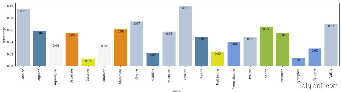
C.2 EMPIRICAL BASELINE Figure 9: Visualization of the estimated empirical distribution for the 20 standard amino acids, colored by their class. Note the consistency with the statistics on the TrEMBL web page.
图 9: 20种标准氨基酸的估计经验分布可视化 (按类别着色)。请注意与TrEMBL网页统计数据的吻合性。
A random baseline, with uniform probability across all the vocabulary tokens at every position, has accuracy $5%$ (when including only the 20 standard amino acids) and $4%$ (when also including the 5 anomalous amino acids (Consortium, 2019)). However, the empirical frequencies of the various amino acids in our dataset may be far from uniform, so we also consider an empirical baseline where the amino acid probabilities are proportional to their empirical frequencies in the training set.
随机基线在所有词汇token的每个位置均匀分布概率,准确率为$5%$(仅包含20种标准氨基酸时)和$4%$(同时包含5种异常氨基酸时)(Consortium, 2019)。然而,我们数据集中各种氨基酸的实际频率可能远非均匀分布,因此我们还考虑了一个经验基线,其中氨基酸概率与其在训练集中的实际频率成正比。
Figure 9 shows the estimated empirical distribution. We use both the standard and anomalous amino acids, and we crop sequences to length 1024 to match the data processing performed for the Transformer models. The figure shows only the 20 standard amino acids, colored by their class, for comparison with the visualization on the TrEMBL web page6.
图 9 展示了估计的经验分布。我们同时使用了标准氨基酸和异常氨基酸,并将序列裁剪至长度 1024 以匹配 Transformer 模型的数据处理流程。图中仅显示 20 种标准氨基酸 (按类别着色) ,以便与 TrEMBL 网页的可视化结果进行对比。
C.3 TABULAR RESULTS
C.3 表格结果
Table 2 contains the results on the single protein sequence modeling task $\begin{array}{r}{Z=1024,}\end{array}$ ). We report accuracy and perplexity as defined in Appendix A:
表 2: 单蛋白质序列建模任务的结果 (Z=1024)。我们按照附录 A 中的定义报告准确率和困惑度:
| Model Type | Set Name | Model | Accuracy | Perplexity |
| UNI | Test | Empirical Baseline Transformer Performer (generalized) | 9.92 30.80 31.58 | 17.80 9.37 9.17 |
| OOD | Empirical Baseline Transformer Performer (generalized) | 9.07 19.70 18.44 | 17.93 13.20 13.63 | |
| BID | Test | Transformer Performer (generalized) Performer (softmax) | 33.32 36.09 33.00 | 9.22 8.36 9.24 |
| OOD | Transformer Performer (generalized) Performer (softmax) | 25.07 24.10 23.48 | 12.09 12.26 12.41 |
Table 2: Results on single protein sequence modeling $\mathit{\Delta}L=1024\rangle$ . We note that the empirical baseline results are applicable to both the unidirectional (UNI) and bidirectional (BID) models.
| 模型类型 | 数据集名称 | 模型 | 准确率 | 困惑度 |
|---|---|---|---|---|
| UNI | Test | 经验基线 Transformer Performer (广义) | 9.92 30.80 31.58 | 17.80 9.37 9.17 |
| UNI | OOD | 经验基线 Transformer Performer (广义) | 9.07 19.70 18.44 | 17.93 13.20 13.63 |
| BID | Test | Transformer Performer (广义) Performer (softmax) | 33.32 36.09 33.00 | 9.22 8.36 9.24 |
| BID | OOD | Transformer Performer (广义) Performer (softmax) | 25.07 24.10 23.48 | 12.09 12.26 12.41 |
表 2: 单蛋白序列建模结果 $\mathit{\Delta}L=1024\rangle$ 。我们注意到经验基线结果同时适用于单向(UNI)和双向(BID)模型。
C.4 ATTENTION MATRIX ILLUSTRATION
C.4 注意力矩阵图示
In this section we illustrate the attention matrices produced by a Performer model. We focus on the bidirectional case and choose one Performer model trained on the standard single-sequence TrEMBL task for over 500K steps. The same analysis can be applied to unidirectional Performers as well.
在本节中,我们将展示由Performer模型生成的注意力矩阵。我们重点关注双向场景,并选择一个在标准单序列TrEMBL任务上训练超过50万步的Performer模型。该分析同样适用于单向Performer模型。
We note that while the Transformer model instantiate s the attention matrix in order to compute the attention output that incorporates the (queries $Q$ , keys $K$ , values $V$ ) triplet (see Eq. 1 in the main paper), the FAVOR mechanism returns the attention output directly (see Algorithm 1). To account for this discrepancy, we extract the attention matrices by applying each attention mechanism twice: once on each original $(Q,K,V)$ triple to obtain the attention output, and once on a modified $(Q,K,V^{\circ})$ triple, where $V^{\circ}$ contains one-hot indicators for each position index, to obtain the attention matrix. The choice of $V^{\circ}$ ensures that the dimension of the attention output is equal to the sequence length, and that a non-zero output on a dimension $i$ can only arise from a non-zero attention weight to the $i^{t h}$ sequence position. Indeed, in the Transformer case, when comparing the output of this procedure with the instantiated attention matrix, the outputs match.
我们注意到,虽然Transformer模型实例化注意力矩阵以计算包含(查询$Q$、键$K$、值$V$)三元组的注意力输出(参见主论文中的公式1),但FAVOR机制直接返回注意力输出(参见算法1)。为了解决这一差异,我们通过两次应用每种注意力机制来提取注意力矩阵:一次对原始$(Q,K,V)$三元组计算注意力输出,另一次对修改后的$(Q,K,V^{\circ})$三元组(其中$V^{\circ}$包含每个位置索引的独热指示符)计算注意力矩阵。选择$V^{\circ}$确保了注意力输出的维度等于序列长度,并且维度$i$上的非零输出只能来自对第$i^{th}$个序列位置的非零注意力权重。实际上,在Transformer案例中,将该过程输出与实例化注意力矩阵进行比较时,两者结果完全匹配。
Attention matrix example. We start by visualizing the attention matrix for an individual protein sequence. We use the BPT1_BOVIN protein sequence7, one of the most extensively studied globular proteins, which contains 100 amino acids. In Figure 10, we show the attention matrices for the first 4 layers. Note that many heads show a diagonal pattern, where each node attends to its neighbors, and some heads show a vertical pattern, where each head attends to the same fixed positions. These patterns are consistent with the patterns found in Transformer models trained on natural language (Kovaleva et al., 2019). In Figure 12 we highlight these attention patterns by focusing on the first 25 tokens, and in Figure 11, we illustrate in more detail two attention heads.
注意力矩阵示例。我们首先可视化单个蛋白质序列的注意力矩阵。以BPT1_BOVIN蛋白序列为例(该序列含100个氨基酸,是研究最广泛的球状蛋白之一),图10展示了前4层的注意力矩阵。值得注意的是,多个注意力头呈现对角线模式(节点关注其相邻节点),部分注意力头则呈现垂直模式(关注固定位置)。这些模式与自然语言训练的Transformer模型中发现的特征一致[20]。图12通过聚焦前25个token突显了这些注意力模式,图11则更详细地展示了两个注意力头的工作机制。
Amino acid similarity. Furthermore, we analyze the amino-acid similarity matrix estimated from the attention matrices produced by the Performer model, as described in Vig et al. (Vig et al., 2020). We aggregate the attention matrix across 800 sequences. The resulting similarity matrix is illustrated in Figure 13. Note that the Performer recognizes highly similar amino acid pairs such as (D, E) and (F, Y).
氨基酸相似性。此外,我们分析了从Performer模型生成的注意力矩阵估计的氨基酸相似性矩阵,如Vig等人所述 (Vig et al., 2020)。我们汇总了800条序列的注意力矩阵,结果相似性矩阵如图13所示。值得注意的是,Performer识别出了高度相似的氨基酸对,例如 (D, E) 和 (F, Y)。
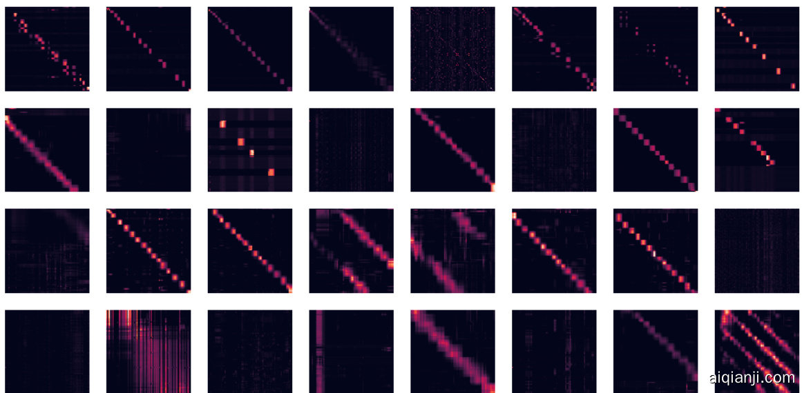

Figure 10: We show the attention matrices for the first 4 layers and all 8 heads (each row is a layer, each column is head index, each cell contains the attention matrix across the entire BPT1_BOVIN protein sequence). Note that many heads show a diagonal pattern, where each node attends to its neighbors, and some heads show a vertical pattern, where each head attends to the same fixed positions. Figure 11: We illustrate in more detail two attention heads. The sub-figures correspond respectively to: (1) Head 1-2 (second layer, third head), (2) Head 4-1 (fifth layer, second head). Note the block attention in Head 1-2 and the vertical attention (to the start token (‘M’) and the 85th token $(\mathrm{\ddot{C}})$ ) in Head 4-1.
图 10: 我们展示了前4层和所有8个注意力头(attention head)的注意力矩阵(attention matrix)(每行代表一个层,每列代表头索引,每个单元格包含整个BPT1_BOVIN蛋白质序列的注意力矩阵)。注意,许多头显示出对角线模式,其中每个节点关注其相邻节点,而一些头显示出垂直模式,其中每个头关注相同的固定位置。
图 11: 我们更详细地展示了两个注意力头。子图分别对应:(1) 头1-2(第二层,第三个头),(2) 头4-1(第五层,第二个头)。注意头1-2中的块注意力(block attention)和头4-1中的垂直注意力(指向起始token('M')和第85个token$(\mathrm{\ddot{C}})$)。
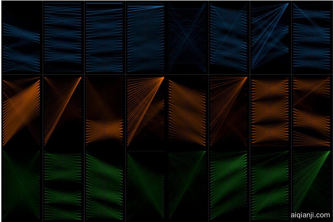
Figure 12: We highlight the attention patterns by restricting our attention to the first 25 tokens (note that we do not re normalize the attention to these tokens). The illustration is based on Vig et al. (Vig, 2019; Vig & Belinkov, 2019). Note that, similar to prior work on protein Transformers (Madani et al., 2020), the attention matrices include both local and global patterns.
图 12: 我们通过将注意力限制在前25个token来突出注意力模式 (注意: 这些token的注意力未重新归一化)。该图示基于Vig等人 (Vig, 2019; Vig & Belinkov, 2019) 的研究。与先前蛋白质Transformer的研究 (Madani et al., 2020) 类似,注意力矩阵同时包含局部和全局模式。
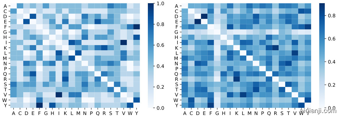
Figure 13: Amino acid similarity matrix estimated from attention matrices aggregated across a small subset of sequences, as described in Vig et al. (Vig et al., 2020). The sub-figures correspond respectively to: (1) the normalized BLOSUM matrix, (2) the amino acid similarity estimated via a trained Performer model. Note that the Performer recognizes highly similar amino acid pairs such as (D, E) and (F, Y).
图 13: 从小规模序列子集聚合的注意力矩阵估计的氨基酸相似性矩阵,如Vig等人所述 (Vig et al., 2020)。子图分别对应:(1) 归一化BLOSUM矩阵,(2) 通过训练后的Performer模型估计的氨基酸相似性。值得注意的是,Performer能识别高度相似的氨基酸对,如(D, E)和(F, Y)。
D EXTENDED APPROXIMATION AND COMPARISON RESULTS
D 扩展近似与比较结果
D.1 BACKWARDS COMPATIBILITY - ERROR PROPAGATION
D.1 向后兼容性 - 错误传播
Although mentioned previously (Sec. 4.2) that the Performer with additional finetuning is backwards compatible with the Transformer, we demonstrate below in Fig. 14 that error propagation due to nonattention components of the Transformer is one of the primary reasons that pretrained Transformer weights cannot be immediately used for inference on the corresponding Performer.
虽然前文(第4.2节)提到经过额外微调的Performer能够向后兼容Transformer,但我们在图14中展示:由于Transformer非注意力组件导致的误差传播,是预训练Transformer权重无法直接用于对应Performer推理的主要原因之一。
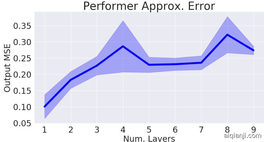
Figure 14: Output approximation errors between a vanilla Transformer and a Performer (with orthogonal features) for varying numbers of layers.
图 14: 普通 Transformer 与 Performer (使用正交特征)在不同层数下的输出近似误差对比。
D.2 APPROXIMATE SOFTMAX - EXTENDED PROPERTIES
D.2 近似Softmax - 扩展特性
We show the following properties of our softmax approximation, in Fig. 15:
我们在图 15 中展示了我们的 softmax 近似方法的以下特性:
Redrawing: While the benefits of redrawing features was shown in Subsec. 4.3 of the main body of the paper, we also demonstrate its benefits when there are multiple layers with large scale (16x16 TPU-v2) training.
重绘:虽然论文主体第4.3小节已展示重绘特征的优势,但我们进一步证明了该技术在多层大规模(16x16 TPU-v2)训练场景下的有效性。
Unidirectional: While we have shown on TrEMBL that Performer with generalized ReLU attention outperforms softmax, we also show that approximate softmax attention can still be a solid choice, for example on ImageNet64 (U). After 100K steps of training, the Performer-ReLU, Performer-Softmax, and Performer-Softmax (SMREG) variants achieve respectively, 3.67, 3.69, 3.67 BPD.
单向性:尽管我们在TrEMBL上证明了采用广义ReLU注意力机制的Performer优于softmax,但我们也表明近似softmax注意力仍不失为一种可靠选择,例如在ImageNet64 (U) 数据集上。经过10万步训练后,Performer-ReLU、Performer-Softmax和Performer-Softmax (SMREG) 变体分别达到3.67、3.69、3.67 BPD。
Instability of Trigonometric Features: We see the full view of the unstable training curve when using Trigonometric softmax.
三角特征的不稳定性:我们观察到使用三角softmax时训练曲线呈现全面不稳定的情况。
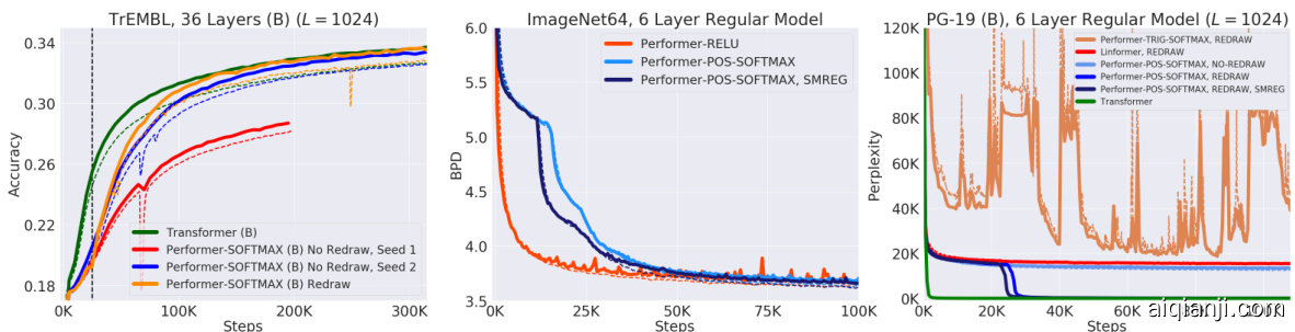
Figure 15: Best viewed zoomed in. Left: The importance of redrawing features. If redrawing is not used, an "unlucky" set of random features may cause training degradation, shown by the early-stopped curve with Seed 1, while a ‘lucky’ set of random features may cause no issue, shown by the curve with Seed 2. Redrawing allows the training to correct itself, as seen at the black vertical line. Middle: Using the same $8\mathrm{x}8$ TPU-v2 compute and same 6-layer standard model, approximate softmax with positive features achieves the same result as generalized ReLU attention. Right: Zoomed out view of right subfigure of Fig. 5, showing that Trigonometric softmax causes very unstable training behaviors.
图 15: 最佳效果需放大查看。左图:特征重绘的重要性。若不使用重绘机制,"不幸"的随机特征组合可能导致训练效果下降(如Seed 1的早停曲线所示),而"幸运"的随机特征组合可能不受影响(如Seed 2曲线所示)。如黑色竖线所示,重绘机制能使训练过程自我修正。中图:在相同$8\mathrm{x}8$ TPU-v2算力与6层标准模型架构下,采用正特征近似softmax与广义ReLU注意力取得同等效果。右图:图5右侧子图的放大视图,显示三角softmax会导致极不稳定的训练行为。
D.3 GENERALIZED ATTENTION
D.3 广义注意力
We investigated Generalized Attention mechanisms (mentioned in Sec. 2.2) on TrEMBL when $L=512$ for various kernel functions. This is similar to (Tsai et al., 2019) which also experiments with various attention kernels for natural language. Using hyper parameter sweeps across multiple variables in FAVOR, we compared several kernels and also re normalization on/off (Fig. 16 and Fig. 17), where Re normalize corresponds to applying $\mathbf{D}^{-1}$ operator in attention, as for the standard mechanism, though we noticed that disabling it does not necessarily hurt accuracy) to produce the best training configuration for the Performer. We note that the effective batch size slightly affects the rankings (as shown by the difference between $2\mathbf{x}2$ and $4\mathbf{x}4$ TPU runs) - we by default use the generalized ReLU kernel with other default hyper parameters shown in Appendix A, as we observed that they are empirically optimal for large batch size runs (i.e. $8\mathrm{x}8$ or 16x16 TPU’s).
我们研究了TrEMBL上广义注意力机制(见2.2节)在$L=512$时针对不同核函数的表现。这与(Tsai et al., 2019)类似,后者也尝试了多种自然语言处理的注意力核函数。通过在FAVOR中对多个变量进行超参数扫描,我们比较了几种核函数以及重归一化开启/关闭的效果(图16和图17),其中重归一化对应在注意力中应用$\mathbf{D}^{-1}$算子(标准机制的做法,但我们发现关闭该操作不一定会降低准确率),从而为Performer确定最佳训练配置。值得注意的是,有效批次大小会略微影响排名(如$2\mathbf{x}2$与$4\mathbf{x}4$ TPU运行的差异所示)——我们默认使用广义ReLU核函数,其他默认超参数见附录A,因为我们观察到这些配置在大批次运行(即$8\mathrm{x}8$或16x16 TPU)中具有经验最优性。
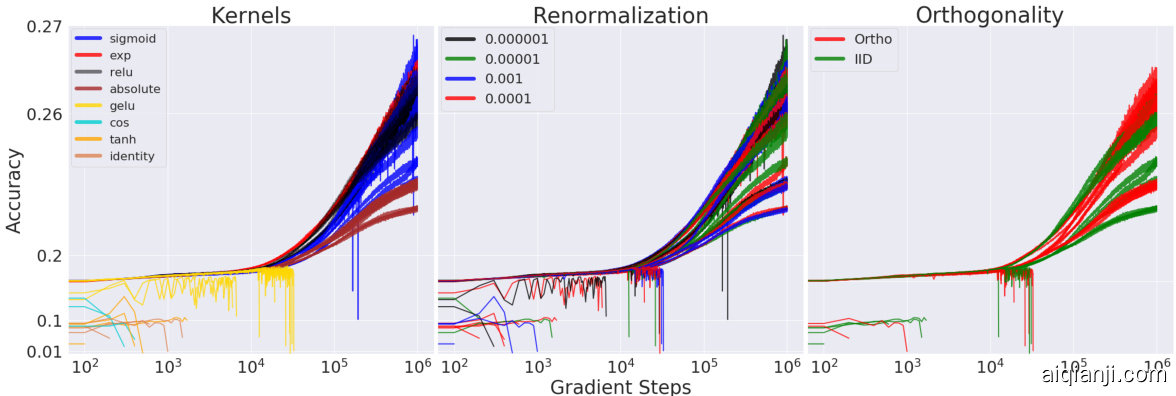

Figure 16: To emphasize the highest accuracy runs but also show the $\mathrm{NaN}$ issues with certain kernels which caused runs to stop early, we set both x and y axes to be log-scale. We tested kernels defined by different functions $f$ (see: Sec. 2.2): sigmoid, exponential, ReLU, absolute, gelu, cosine (original softmax approximation), tanh, and identity. All training runs were performed on $2\mathrm{x}2$ TPU-v2’s, 128 batch size per device.
图 16: 为突出最高准确率的运行结果,同时展示某些内核因 $\mathrm{NaN}$ 问题导致运行提前终止的情况,我们将x轴和y轴均设为对数尺度。测试了由不同函数 $f$ 定义的内核 (参见第2.2节): sigmoid、exponential、ReLU、absolute、gelu、cosine (原始softmax近似)、tanh以及identity。所有训练均在 $2\mathrm{x}2$ TPU-v2设备上完成,每设备批处理大小为128。
D.4 COMPARISON WITH LINEAR TRANSFORMER
D.4 与线性 Transformer 的对比
We use the attention implementation of the Linear Transformer from (Katha ro poul os et al., 2020), which mainly involves setting our feature map $\phi(x)=\mathrm{elu}(x)+1$ , where $\operatorname{elu}(x)$ is the shifted-eLU function from (Clevert et al., 2016).
我们采用了 (Katharopoulos et al., 2020) 提出的线性 Transformer (Linear Transformer) 注意力实现方案,其核心在于将特征映射设为 $\phi(x)=\mathrm{elu}(x)+1$ ,其中 $\operatorname{elu}(x)$ 来自 (Clevert et al., 2016) 提出的平移指数线性单元函数。
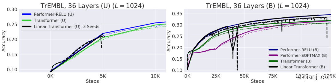
Figure 17: We also performed a similar setup as Fig. 16 for $4\mathbf{x}4$ TPU-v2’s. Figure 18: Left: In the unidirectional 36-ProGen setting, we ran 3 seeds of the Linear Transformer, and found that all 3 seeds produced exploding gradients very early on, stopping the training run. Right: The Linear Transformer in the bidirectional setting also produced an exploding gradient in the middle of training, near 125K steps. Exploding gradients can be evidenced by the sharp drop in train accuracy right before a NaN error.
图 17: 我们在 $4\mathbf{x}4$ TPU-v2 上进行了与图 16 类似的实验设置。
图 18: 左图: 在单向 36-ProGen 设置中,我们对 Linear Transformer 进行了 3 次随机种子实验,发现所有 3 次实验都在早期出现梯度爆炸,导致训练中止。右图: 双向设置中的 Linear Transformer 在训练中期约 125K 步时也出现了梯度爆炸。梯度爆炸可通过 NaN 错误前训练准确率的急剧下降来验证。
For the sake of fairness and to prevent confounding results, while (Katha ro poul os et al., 2020) also uses the GeLU non linearity for the MLPs in the Linear Transformer, we instead use the original ReLU non linearity. We also used the exact same training hyper parameters as Performer-ReLU on our exact ProGen setting from Fig. 6. Ultimately, we empirically found that the Linear Transformer possessed numerical instability during training via unstable training curves, ultimately stopping training by producing exploding gradients (NaNs) (Fig. 18).
为了公平性并防止结果混淆,尽管 (Katha ro poul os et al., 2020) 在 Linear Transformer 的 MLP 中也使用了 GeLU 非线性激活函数,但我们仍采用原始的 ReLU 非线性激活函数。我们还使用了与图 6 中 ProGen 设定完全相同的训练超参数(与 Performer-ReLU 一致)。最终,我们通过实验发现 Linear Transformer 在训练过程中存在数值不稳定性,表现为不稳定的训练曲线,最终因梯度爆炸(NaN)而终止训练(图 18)。
D.5 LONG RANGE ARENA
D.5 长程竞技场
Performers are compared against many additional (scalable and not scalable) methods not included in our paper: Local Attention, Sparse Attention, Longformer, Sinkhorn Transformer, Synthesizer, Big Bird and the aforementioned Linear Transformer on challenging long range context tasks in the Long Range Arena (Tay et al., 2021), with Fig. 19 displaying the original paper’s results. Performers obtain the largest LRA (Long Range Arena) score among all tested scalable Transformers methods (which we define by having speed of $>100$ examples/sec).
Performers 与许多未包含在我们论文中的其他(可扩展和不可扩展)方法进行了比较:Local Attention、Sparse Attention、Longformer、Sinkhorn Transformer、Synthesizer、Big Bird 以及前述的 Linear Transformer,在 Long Range Arena (Tay et al., 2021) 的挑战性长程上下文任务中进行了测试,图 19 展示了原始论文的结果。Performers 在所有测试的可扩展 Transformer 方法(我们定义为速度 >100 样本/秒)中获得了最高的 LRA (Long Range Arena) 分数。
Tasks used for comparison include: (1) a longer variation of the standard ListOps task proposed in (Nangia & Bowman, 2018), (2) byte-level text classification using real-world data, (3) byte-level document retrieval, (4) image classification on sequences of pixels, and (5) Pathfinder task (longrange spatial dependency problem). In the Long Range Arena paper, the authors found that all models do not learn anything on Path-X task (denoted by FAIL), contrary to the Pathfinder task, which shows that increasing the sequence length can cause seriously difficulties for model training.
用于对比的任务包括:(1) (Nangia & Bowman, 2018) 提出的标准ListOps任务的长序列变体,(2) 基于真实数据的字节级文本分类,(3) 字节级文档检索,(4) 像素序列图像分类,以及(5) Pathfinder任务(长程空间依赖问题)。在Long Range Arena论文中,作者发现所有模型在Path-X任务(标记为FAIL)上均未学到有效特征,这与Pathfinder任务的表现形成鲜明对比,表明序列长度的增加会给模型训练带来严重困难。

Figure 19: Upper Table: Results on Long-Range Arena benchmark. Best model is in boldface and second best is underlined. Lower Table: Benchmark results of all X-former models with a consistent batch size of 32 across all models. The authors report relative speed increase/decrease in comparison with the vanilla Transformer in brackets besides the steps per second. Memory usage refers to per device memory usage across each TPU device. Benchmarks are run on $4\mathbf{x}4$ TPU-v3 chips. Right Fig: Performance (y-axis), speed ( $\mathbf{\rho}_{\mathrm{{X}}}$ -axis), and memory footprint (size of the circles) of different models.
图 19: 上表: Long-Range Arena基准测试结果。最佳模型以粗体显示,次优模型带下划线。下表: 所有X-former模型在批量大小统一为32时的基准测试结果。作者在每秒步数旁用括号标注了与原始Transformer (vanilla Transformer) 相比的相对速度增减。内存使用量指每个TPU设备的单设备内存占用。基准测试在$4\mathbf{x}4$ TPU-v3芯片上运行。右图: 不同模型的性能(y轴)、速度($\mathbf{\rho}_{\mathrm{{X}}}$轴)和内存占用(圆圈大小)。
E COMPUTATION COSTS - EXTENDED RESULTS
E 计算成本 - 扩展结果
In this subsection, we empirically measure computational costs in terms wall clock time on forward and backward passes for three scenarios in Fig. 20:
在本小节中,我们通过实验测量了图20中三种场景下前向传播和反向传播的实际耗时:
Since some of the computational bottleneck in the Transformer may originate from the extra feed-forward layers (Kitaev et al., 2020), we also benchmark the “Small" version, i.e. $(n_{h e a d s},n_{l a y e r s},d_{f f},d)=(1,6,64,64)$ as well, when the attention component is the dominant source of computation and memory. We remind the reader that the “Regular" version consists of $(n_{h e a d s},n_{l a y e r s},d_{f f},d)=(8,6,2048,512).$
由于Transformer中的部分计算瓶颈可能源于额外的前馈层 (Kitaev et al., 2020),我们还对"Small"版本 $(n_{heads},n_{layers},d_{ff},d)=(1,6,64,64)$ 进行了基准测试,此时注意力组件成为计算和内存的主要来源。需要提醒读者的是,"Regular"版本的配置为 $(n_{heads},n_{layers},d_{ff},d)=(8,6,2048,512)$。

Figure 20: Captions (1) and (2) for each $2\mathbf{x}2$ subfigure mentioned above.
图 20: 上述每个 $2\mathbf{x}2$ 子图的标题 (1) 和 (2)。
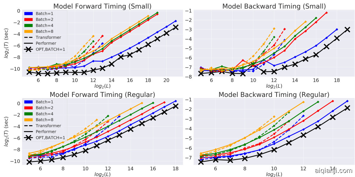
Figure 21: Caption (3) for this $2\mathbf{x}2$ subfigure mentioned above.
图 21: 上述 $2\mathbf{x}2$ 子图的标题 (3)。
F THEORETICAL RESULTS
F 理论结果
We provide here the proofs of all theoretical results presented in the paper.
我们在此提供论文中所有理论结果的证明。
F.1 PROOF OF LEMMA 1
F.1 引理1的证明
Proof. We first deduce that for any $\pmb{a},\pmb{b}\in\mathbb{R}^{d}$
证明。我们首先推导出对于任意 $\pmb{a},\pmb{b}\in\mathbb{R}^{d}$
$$
\operatorname{SM}(\mathbf{x},\mathbf{y})=\exp({\mathbf{x}^{\top}\mathbf{y}})=\exp(-|{\boldsymbol{\mathbf{x}}}|^{2}/2)\cdot\exp(|{\boldsymbol{\mathbf{x}}}+{\boldsymbol{\mathbf{y}}}|^{2}/2)\cdot\exp(-|{\boldsymbol{\mathbf{y}}}|^{2}/2).
$$
$$
\operatorname{SM}(\mathbf{x},\mathbf{y})=\exp({\mathbf{x}^{\top}\mathbf{y}})=\exp(-|{\boldsymbol{\mathbf{x}}}|^{2}/2)\cdot\exp(|{\boldsymbol{\mathbf{x}}}+{\boldsymbol{\mathbf{y}}}|^{2}/2)\cdot\exp(-|{\boldsymbol{\mathbf{y}}}|^{2}/2).
$$
Next, let $\boldsymbol{w}\in\mathbb{R}^{d}$ . We use the fact that
接下来,令 $\boldsymbol{w}\in\mathbb{R}^{d}$。我们利用以下事实:
$$
(2\pi)^{-d/2}\int\exp(-|\pmb{w}-\pmb{c}|_{2}^{2}/2)d\pmb{w}=1
$$
$$
(2\pi)^{-d/2}\int\exp(-|\pmb{w}-\pmb{c}|_{2}^{2}/2)d\pmb{w}=1
$$
for any $\pmb{c}\in\mathbb{R}^{d}$ and derive:
对于任意 $\pmb{c}\in\mathbb{R}^{d}$,并推导出:
$$
\begin{array}{r l}&{\exp(|x+y|^{2}/2)=(2\pi)^{-d/2}\exp(|x+y|^{2}/2)\int\exp(-|w-(x+y)|^{2}/2)d w}\ &{\qquad=(2\pi)^{-d/2}\int\exp(-|w|^{2}/2+w^{\top}(x+y)-|x+y|^{2}/2+|x+y|^{2}/2)d w}\ &{\qquad=(2\pi)^{-d/2}\int\exp(-|w|^{2}/2+w^{\top}(x+y))d w}\ &{\qquad=(2\pi)^{-d/2}\int\exp(-|w|^{2}/2)\cdot\exp(w^{\top}x)\cdot\exp(w^{\top}y)d w}\ &{\qquad=\mathbb{E}_ {w\sim N(0_{d},\mathbb{L}_{1})}[\exp(\omega^{\top}x)\cdot\exp(\omega^{\top}y)].}\end{array}
$$
$$
\begin{array}{r l}&{\exp(|x+y|^{2}/2)=(2\pi)^{-d/2}\exp(|x+y|^{2}/2)\int\exp(-|w-(x+y)|^{2}/2)d w}\ &{\qquad=(2\pi)^{-d/2}\int\exp(-|w|^{2}/2+w^{\top}(x+y)-|x+y|^{2}/2+|x+y|^{2}/2)d w}\ &{\qquad=(2\pi)^{-d/2}\int\exp(-|w|^{2}/2+w^{\top}(x+y))d w}\ &{\qquad=(2\pi)^{-d/2}\int\exp(-|w|^{2}/2)\cdot\exp(w^{\top}x)\cdot\exp(w^{\top}y)d w}\ &{\qquad=\mathbb{E}_ {w\sim N(0_{d},\mathbb{L}_{1})}[\exp(\omega^{\top}x)\cdot\exp(\omega^{\top}y)].}\end{array}
$$
That completes the proof of the first part of the lemma. An identity involving hyperbolic cosine function is implied by the fact that for every $\mathbf{u}\in\mathbb{R}^{d}$ and $\omega\sim\mathcal{N}(0,\dot{\bf I}_{d})$ the following is true:
至此完成了引理第一部分的证明。根据以下事实可推出一个涉及双曲余弦函数的恒等式:对于任意 $\mathbf{u}\in\mathbb{R}^{d}$ 和 $\omega\sim\mathcal{N}(0,\dot{\bf I}_{d})$ ,下式成立:
$$
\mathbb{E}[\exp(\omega^{\top}\mathbf{u})]=\sum_{i=0}^{\infty}\frac{\mathbb{E}[(\omega^{\top}\mathbf{u})^{2i}]}{(2i)!}=\frac{1}{2}\sum_{i=0}^{\infty}\frac{\mathbb{E}[(\omega^{\top}\mathbf{u})^{2i}]+\mathbb{E}[(-\omega^{\top}\mathbf{u})^{2i}]}{(2i)!}.
$$
$$
\mathbb{E}[\exp(\omega^{\top}\mathbf{u})]=\sum_{i=0}^{\infty}\frac{\mathbb{E}[(\omega^{\top}\mathbf{u})^{2i}]}{(2i)!}=\frac{1}{2}\sum_{i=0}^{\infty}\frac{\mathbb{E}[(\omega^{\top}\mathbf{u})^{2i}]+\mathbb{E}[(-\omega^{\top}\mathbf{u})^{2i}]}{(2i)!}.
$$
The cancellation of the odd moments $\mathbb{E}[(\omega^{\top}\mathbf u)^{2i+1}]$ follows directly from the fact that $\omega$ is taken from the isotropic distribution (i.e. distribution with pdf function constant on each sphere). That completes the proof.口
奇数阶矩 $\mathbb{E}[(\omega^{\top}\mathbf u)^{2i+1}]$ 的消除直接源于 $\omega$ 取自各向同性分布(即概率密度函数在每个球面上保持恒定的分布)。至此证明完成。
F.2 PROOF OF LEMMA 2
F.2 引理2的证明
Proof. Denote: ${\bf z}={\bf x}+{\bf y}$ and $\Delta={\bf x}-{\bf y}$ . Note that by using standard trigonometric identities (and the fact that the variance of the sum of independent random variables is the sum of variances of those random variables), we can get the following for $\omega\sim\mathcal{N}(0,\mathbf{I}_{d})$ :
证明。记:${\bf z}={\bf x}+{\bf y}$ 且 $\Delta={\bf x}-{\bf y}$。注意到通过标准三角恒等式(以及独立随机变量和的方差等于这些随机变量方差之和的性质),对于 $\omega\sim\mathcal{N}(0,\mathbf{I}_{d})$ 可得:
$$
\operatorname{MSE}({\widehat{\operatorname{SM}}}_{m}^{\operatorname{trig}}(\mathbf{x},\mathbf{y}))={\frac{1}{m}}\exp(|\mathbf{x}|^{2}+|\mathbf{y}|^{2})\operatorname{Var}(\cos(\omega^{\top}\Delta)).
$$
$$
\operatorname{MSE}({\widehat{\operatorname{SM}}}_{m}^{\operatorname{trig}}(\mathbf{x},\mathbf{y}))={\frac{1}{m}}\exp(|\mathbf{x}|^{2}+|\mathbf{y}|^{2})\operatorname{Var}(\cos(\omega^{\top}\Delta)).
$$
Using the fact that (see: Lemma 1 in ( $\mathrm{Yu}$ et al., 2016); note that in that lemma they use notation: $z$ for what we denote as: $\lvert\lvert\Delta\rvert\rvert)$ :
利用以下事实(参见: (Yu 等人, 2016) 中的引理 1;注意该引理使用符号 $z$ 表示我们记为 $\lvert\lvert\Delta\rvert\rvert$ 的量):
$$
\operatorname{Var}(\cos(\omega^{\top}\Delta))=\frac{1}{2}(1-\exp(-|\Delta|^{2}))^{2},
$$
$$
\operatorname{Var}(\cos(\omega^{\top}\Delta))=\frac{1}{2}(1-\exp(-|\Delta|^{2}))^{2},
$$
we obtain:
我们得到:
$$
\begin{array}{r}{\mathrm{MSE}(\widehat{\mathrm{SM}}_{m}^{\mathrm{trig}}({\bf x},{\bf y}))=\displaystyle\frac{1}{2m}\exp(|{\bf x}|^{2}+|{\bf y}|^{2})(1-\exp(-|\Delta|^{2}))^{2}=}\ {\displaystyle\frac{1}{2m}\exp(|{\bf z}|^{2})\mathrm{SM}^{-2}({\bf x},{\bf y})(1-\exp(-|\Delta|^{2}))^{2},}\end{array}
$$
$$
\begin{array}{r}{\mathrm{MSE}(\widehat{\mathrm{SM}}_{m}^{\mathrm{trig}}({\bf x},{\bf y}))=\displaystyle\frac{1}{2m}\exp(|{\bf x}|^{2}+|{\bf y}|^{2})(1-\exp(-|\Delta|^{2}))^{2}=}\ {\displaystyle\frac{1}{2m}\exp(|{\bf z}|^{2})\mathrm{SM}^{-2}({\bf x},{\bf y})(1-\exp(-|\Delta|^{2}))^{2},}\end{array}
$$
which completes the first part of the proof. To obtain the formula for: $\widehat{\mathrm{MSE}(\widehat{\mathrm{SM}}_{m}^{+}(\mathbf{x},\mathbf{y}))}$ notice first that:
这就完成了证明的第一部分。为了得到以下公式:$\widehat{\mathrm{MSE}(\widehat{\mathrm{SM}}_{m}^{+}(\mathbf{x},\mathbf{y}))}$,首先注意到:
$$
\mathbb{E}_ {\omega\sim\mathcal{N}(0,\mathbf{I}_{d})}[\exp(\omega^{\top}\mathbf{z})]=\exp(\frac{|\mathbf{z}|^{2}}{2}).
$$
$$
\mathbb{E}_ {\omega\sim\mathcal{N}(0,\mathbf{I}_{d})}[\exp(\omega^{\top}\mathbf{z})]=\exp(\frac{|\mathbf{z}|^{2}}{2}).
$$
The above immediately follows from the fact that positive random feature maps provide unbiased estimation of the softmax-kernel, thus the following is true:
上述结论直接源于正随机特征映射能够无偏估计 softmax 核函数,因此以下等式成立:
$$
\operatorname{SM}(\mathbf{x},\mathbf{y})=\exp(-\frac{|\mathbf{x}|^{2}+|\mathbf{y}|^{2}}{2})\mathbb{E}_ {\omega\sim\mathcal{N}(0,\mathbf{I}_{d})}[\exp(\omega^{\top}\mathbf{z})].
$$
$$
\operatorname{SM}(\mathbf{x},\mathbf{y})=\exp(-\frac{|\mathbf{x}|^{2}+|\mathbf{y}|^{2}}{2})\mathbb{E}_ {\omega\sim\mathcal{N}(0,\mathbf{I}_{d})}[\exp(\omega^{\top}\mathbf{z})].
$$
Therefore we obtain:
因此我们得到:
$$
\begin{array}{r}{\mathrm{MSE}(\widehat{\mathrm{SM}}_{m}^{+}({\bf x},{\bf y}))=\displaystyle\frac{1}{m}\exp(-(|{\bf x}|^{2}+|{\bf y}|^{2}))\mathrm{Var}(\exp(\omega^{\top}{\bf z}))=}\ {\displaystyle\frac{1}{m}\exp(-(|{\bf x}|^{2}+|{\bf y}|^{2}))\left(\mathbb{E}[\exp(2\omega^{\top}{\bf z})]-(\mathbb{E}[\exp(\omega^{\top}{\bf z})])^{2}\right)=}\ {\displaystyle\frac{1}{m}\exp(-(|{\bf x}|^{2}+|{\bf y}|^{2}))(\exp(2|{\bf z}|^{2})-\exp(|{\bf z}|^{2})),}\end{array}
$$
$$
\begin{array}{r}{\mathrm{MSE}(\widehat{\mathrm{SM}}_{m}^{+}({\bf x},{\bf y}))=\displaystyle\frac{1}{m}\exp(-(|{\bf x}|^{2}+|{\bf y}|^{2}))\mathrm{Var}(\exp(\omega^{\top}{\bf z}))=}\ {\displaystyle\frac{1}{m}\exp(-(|{\bf x}|^{2}+|{\bf y}|^{2}))\left(\mathbb{E}[\exp(2\omega^{\top}{\bf z})]-(\mathbb{E}[\exp(\omega^{\top}{\bf z})])^{2}\right)=}\ {\displaystyle\frac{1}{m}\exp(-(|{\bf x}|^{2}+|{\bf y}|^{2}))(\exp(2|{\bf z}|^{2})-\exp(|{\bf z}|^{2})),}\end{array}
$$
where the last equality follows from Equation 16. Therefore we have:
最后一个等式由方程 16 得出。因此我们有:
$$
\small\begin{array}{r}{\mathrm{MSE}(\widehat{\mathrm{SM}}_{m}^{+}({\bf x},{\bf y}))=\displaystyle\frac{1}{m}\exp(-(|{\bf x}|^{2}+|{\bf y}|^{2}))\exp(|{\bf z}|^{2})(\exp(|{\bf z}|^{2})-1)=}\ {\displaystyle\frac{1}{m}\exp(|{\bf z}|^{2})\mathrm{SM}^{2}({\bf x},{\bf y})(1-\exp(-|{\bf z}|^{2})).}\end{array}
$$
$$
\small\begin{array}{r}{\mathrm{MSE}(\widehat{\mathrm{SM}}_{m}^{+}({\bf x},{\bf y}))=\displaystyle\frac{1}{m}\exp(-(|{\bf x}|^{2}+|{\bf y}|^{2}))\exp(|{\bf z}|^{2})(\exp(|{\bf z}|^{2})-1)=}\ {\displaystyle\frac{1}{m}\exp(|{\bf z}|^{2})\mathrm{SM}^{2}({\bf x},{\bf y})(1-\exp(-|{\bf z}|^{2})).}\end{array}
$$
Finally,
最后,
$$
\begin{array}{r l r}&{}&{\mathrm{MSE}(\widehat{\mathbf{SM}}_ {m}^{\mathrm{pp+}}(\mathbf{x},\mathbf{y}))=\frac{1}{4m}\exp(-\frac{|\mathbf{x}|^{2}+|\mathbf{y}|^{2}}{2})^{2}(\mathrm{Var}(\exp({\omega}^{\top}\mathbf{z}))+\mathrm{Var}(\exp(-{\omega}^{\top}\mathbf{z}))+}\ &{}&{2\mathrm{Cov}(\exp({\omega}^{\top}\mathbf{z})),\exp(-{\omega}^{\top}\mathbf{z}))))=\frac{1}{4m}\exp(-\frac{|\mathbf{x}|^{2}+|\mathbf{y}|^{2}}{2})^{2}(2\mathrm{Var}(\exp({\omega}^{\top}\mathbf{z}))+}\ &{}&{2\mathrm{Cov}(\exp({\omega}^{\top}\mathbf{z})),\exp(-{\omega}^{\top}\mathbf{z}))))=\frac{1}{2m}\exp(-(|\mathbf{x}|^{2}+|\mathbf{y}|^{2}))}\ &{}&{(\mathrm{Var}(\exp({\omega}^{\top}\mathbf{z}))+1-(\mathbb{E}[\exp({\omega}^{\top}\mathbf{z})])^{2})=\frac{1}{2m}\exp(-(|\mathbf{x}|^{2}+|\mathbf{y}|^{2}))}\ &{}&{(\exp(2|\mathbf{z}|^{2})-\exp(|\mathbf{z}|^{2})+1-\exp(|\mathbf{z}|^{2}))=\frac{1}{2m}\exp(-(|\mathbf{x}|^{2}+|\mathbf{y}|^{2}))(\exp(|\mathbf{z}|^{2})-1)^{2}}\ &{}&{=\frac{1}{2}(1-\exp(-|\mathbf{z}|^{2}))\mathrm{MSE}(\widehat{\mathbf{SM}}_{m}^{+}(\mathbf{x},\mathbf{y})).}\end{array}
$$
$$
\begin{array}{r l r}&{}&{\mathrm{MSE}(\widehat{\mathbf{SM}}_ {m}^{\mathrm{pp+}}(\mathbf{x},\mathbf{y}))=\frac{1}{4m}\exp(-\frac{|\mathbf{x}|^{2}+|\mathbf{y}|^{2}}{2})^{2}(\mathrm{Var}(\exp({\omega}^{\top}\mathbf{z}))+\mathrm{Var}(\exp(-{\omega}^{\top}\mathbf{z}))+}\ &{}&{2\mathrm{Cov}(\exp({\omega}^{\top}\mathbf{z})),\exp(-{\omega}^{\top}\mathbf{z}))))=\frac{1}{4m}\exp(-\frac{|\mathbf{x}|^{2}+|\mathbf{y}|^{2}}{2})^{2}(2\mathrm{Var}(\exp({\omega}^{\top}\mathbf{z}))+}\ &{}&{2\mathrm{Cov}(\exp({\omega}^{\top}\mathbf{z})),\exp(-{\omega}^{\top}\mathbf{z}))))=\frac{1}{2m}\exp(-(|\mathbf{x}|^{2}+|\mathbf{y}|^{2}))}\ &{}&{(\mathrm{Var}(\exp({\omega}^{\top}\mathbf{z}))+1-(\mathbb{E}[\exp({\omega}^{\top}\mathbf{z})])^{2})=\frac{1}{2m}\exp(-(|\mathbf{x}|^{2}+|\mathbf{y}|^{2}))}\ &{}&{(\exp(2|\mathbf{z}|^{2})-\exp(|\mathbf{z}|^{2})+1-\exp(|\mathbf{z}|^{2}))=\frac{1}{2m}\exp(-(|\mathbf{x}|^{2}+|\mathbf{y}|^{2}))(\exp(|\mathbf{z}|^{2})-1)^{2}}\ &{}&{=\frac{1}{2}(1-\exp(-|\mathbf{z}|^{2}))\mathrm{MSE}(\widehat{\mathbf{SM}}_{m}^{+}(\mathbf{x},\mathbf{y})).}\end{array}
$$
In the chain of equalities above we used the fact that random variables $\exp(\boldsymbol{\omega}^{\top}{\mathbf z})$ and $\exp(-\omega^{\top}{\mathbf z})$ have the same distribution. This is true since $\omega$ and $-\omega$ have the same distribution ( $\omega$ is Gaussian). That completes the proof.口
在上述等式链中,我们利用了随机变量 $\exp(\boldsymbol{\omega}^{\top}{\mathbf z})$ 和 $\exp(-\omega^{\top}{\mathbf z})$ 具有相同分布这一事实。这是因为 $\omega$ 和 $-\omega$ 具有相同分布 ( $\omega$ 服从高斯分布)。至此证明完成。
F.3 PROOF OF THEOREM 1
F.3 定理1的证明
Proof. Let x, $\mathbf{\nabla},\mathbf{y}\in\mathbb{R}^{d}$ be respectively a query/key. Note that from the definition of $\mathrm{SMREG}(\mathbf{x},\mathbf{y})$ we have for z = x + y:
证明。设x、$\mathbf{\nabla},\mathbf{y}\in\mathbb{R}^{d}$分别为查询/键。注意到根据$\mathrm{SMREG}(\mathbf{x},\mathbf{y})$的定义,对于z = x + y有:
$$
\mathrm{SMREG}(\mathbf{x},\mathbf{y})=\exp(-\frac{|\mathbf{x}|^{2}+|\mathbf{y}|^{2}}{2})\sum_{k=0}^{\infty}\frac{1}{(2k)!}|\mathbf{z}|^{2k}d^{k}\mathbb{E}_ {\omega\sim\mathcal{N}(0,\mathbf{I}_{d})}[(\frac{\omega}{|\omega|_ {2}}\mathbf{e}_{1})^{2k}],
$$
$$
\mathrm{SMREG}(\mathbf{x},\mathbf{y})=\exp(-\frac{|\mathbf{x}|^{2}+|\mathbf{y}|^{2}}{2})\sum_{k=0}^{\infty}\frac{1}{(2k)!}|\mathbf{z}|^{2k}d^{k}\mathbb{E}_ {\omega\sim\mathcal{N}(0,\mathbf{I}_ {d})}[(\frac{\omega}{|\omega|_ {2}}\mathbf{e}_{1})^{2k}],
$$
where $\mathbf{e}_ {1}\stackrel{\mathrm{def}}{=}(1,0,...,0)^{\top}\in\mathbb{R}^{d}$ . To obtain the above we used the fact that $\mathcal{N}(0,\mathbf{I}_{d})$ is isotropic (that in particular implies zeroing of the even terms in the Taylor expansion).
其中 $\mathbf{e}_ {1}\stackrel{\mathrm{def}}{=}(1,0,...,0)^{\top}\in\mathbb{R}^{d}$ 。推导上式时利用了 $\mathcal{N}(0,\mathbf{I}_{d})$ 具有各向同性这一性质 (该性质使得泰勒展开式中的偶次项为零) 。
Let us denote: $\begin{array}{r}{A(k,d)\stackrel{\mathrm{def}}{=}\mathbb{E}_ {\omega\sim\mathcal{N}(0,\mathbf{I}_ {d})}[\big(\frac{\omega}{|\omega|_ {2}}\mathbf{e}_{1}\big)^{2k}]}\end{array}$ . It turns out that:
让我们定义:$\begin{array}{r}{A(k,d)\stackrel{\mathrm{def}}{=}\mathbb{E}_ {\omega\sim\mathcal{N}(0,\mathbf{I}_ {d})}[\big(\frac{\omega}{|\omega|_ {2}}\mathbf{e}_{1}\big)^{2k}]}\end{array}$。事实证明:
$$
A(2k,d)=\frac{(2k-1)!!}{(d+2k-2)(d+2k-4)\cdot...\cdot d}.
$$
$$
A(2k,d)=\frac{(2k-1)!!}{(d+2k-2)(d+2k-4)\cdot...\cdot d}.
$$
The proof of that fact can be found in the supplement of (Cho roman ski et al., 2018b), yet we provide it below for completeness and the convenience of the Reader:
该证明可在 (Cho roman ski et al., 2018b) 的补充材料中找到,但为了完整性和读者便利性,我们仍在此提供:
Lemma 3. Expression $A(2k,d)$ satisfies the following for $k\in\mathbb N$ :
引理3. 表达式 $A(2k,d)$ 对于 $k\in\mathbb N$ 满足以下条件:
$$
A(2k,d)=\frac{(2k-1)!!}{(d+2k-2)(d+2k-4)\cdot...\cdot d}.
$$
$$
A(2k,d)=\frac{(2k-1)!!}{(d+2k-2)(d+2k-4)\cdot...\cdot d}.
$$
Proof. Note first that for $d\geq2$ the density function $p_{d}(\theta)$ of the angle between a vector $\mathbf{r}\in\mathbb{R}^{d}$ chosen uniformly at random from the unit sphere and $\mathbf{e}_{1}$ is given by the following formula:
证明。首先注意到对于 $d\geq2$,从单位球面上均匀随机选取的向量 $\mathbf{r}\in\mathbb{R}^{d}$ 与 $\mathbf{e}_ {1}$ 之间夹角的密度函数 $p_{d}(\theta)$ 由以下公式给出:
$$
p_{d}(\theta)=\frac{\sin^{d-2}(\theta)}{\int_{0}^{\pi}\sin^{d-2(\theta)}d\theta}.
$$
$$
p_{d}(\theta)=\frac{\sin^{d-2}(\theta)}{\int_{0}^{\pi}\sin^{d-2(\theta)}d\theta}.
$$
Let us denote: $\begin{array}{r}{F(k,d)\stackrel{\mathrm{def}}{=}\int_{0}^{\pi}\cos^{k}(\theta)\sin^{d}(\theta)d\theta}\end{array}$ . Using partial integration, we get:
我们定义:$\begin{array}{r}{F(k,d)\stackrel{\mathrm{def}}{=}\int_{0}^{\pi}\cos^{k}(\theta)\sin^{d}(\theta)d\theta}\end{array}$。通过分部积分可得:
$$
\begin{array}{r}{\displaystyle\int_{0}^{\pi}\cos^{k}(\theta)\sin^{d}(\theta)d\theta=\displaystyle\int_{0}^{\pi}\cos^{k-1}(\theta)\sin^{d}(\theta)(\sin(\theta))^{\prime}d\theta=}\ {\displaystyle\cos^{k-1}(\theta)\sin^{d+1}(\theta)|_ {0}^{\pi}-\displaystyle\int_{0}^{\pi}\sin(\theta)((k-1)\cos^{k-2}(\theta)(-\sin(\theta))\sin^{d}(\theta)+}\ {\displaystyle d\cos^{k}(\theta)\sin^{d-1}(\theta))d\theta.}\end{array}
$$
$$
\begin{array}{r}{\displaystyle\int_{0}^{\pi}\cos^{k}(\theta)\sin^{d}(\theta)d\theta=\displaystyle\int_{0}^{\pi}\cos^{k-1}(\theta)\sin^{d}(\theta)(\sin(\theta))^{\prime}d\theta=}\ {\displaystyle\cos^{k-1}(\theta)\sin^{d+1}(\theta)|_ {0}^{\pi}-\displaystyle\int_{0}^{\pi}\sin(\theta)((k-1)\cos^{k-2}(\theta)(-\sin(\theta))\sin^{d}(\theta)+}\ {\displaystyle d\cos^{k}(\theta)\sin^{d-1}(\theta))d\theta.}\end{array}
$$
Thus we conclude that: $\textstyle F(k,d)={\frac{k-1}{d+1}}F(k-2,d+2)$ . Therefore we have:
因此我们得出:$\textstyle F(k,d)={\frac{k-1}{d+1}}F(k-2,d+2)$。因此我们有:
$$
F(2k,d)=\frac{(2k-1)!!}{(d+1)(d+3)\cdot\ldots\cdot(d+2k-1)}\int_{0}^{\pi}\sin^{d+2k}(\theta)d\theta.
$$
$$
F(2k,d)=\frac{(2k-1)!!}{(d+1)(d+3)\cdot\ldots\cdot(d+2k-1)}\int_{0}^{\pi}\sin^{d+2k}(\theta)d\theta.
$$
We again conduct partial integration and get:
我们再次进行部分积分得到:
$$
\begin{array}{r}{\displaystyle\int_{0}^{\pi}\sin^{d}(\theta)d\theta=-\frac{1}{d}\sin^{d-1}(\theta)\cos(\theta)|_ {0}^{\pi}+}\ {\displaystyle\frac{d-1}{d}\displaystyle\int_{0}^{\pi}\sin^{d-2}(\theta)d\theta=\frac{d-1}{d}\displaystyle\int_{0}^{\pi}\sin^{d-2}(\theta)d\theta.}\end{array}
$$
$$
\begin{array}{r}{\displaystyle\int_{0}^{\pi}\sin^{d}(\theta)d\theta=-\frac{1}{d}\sin^{d-1}(\theta)\cos(\theta)|_ {0}^{\pi}+}\ {\displaystyle\frac{d-1}{d}\displaystyle\int_{0}^{\pi}\sin^{d-2}(\theta)d\theta=\frac{d-1}{d}\displaystyle\int_{0}^{\pi}\sin^{d-2}(\theta)d\theta.}\end{array}
$$
Therefore we conclude that:
因此我们得出结论:
$$
A(2k,d)={\frac{1}{{\frac{d-3}{d-2}}{\frac{d-5}{d-4}}\cdot\ldots}}{\frac{(2k-1)!!}{(d-1)(d+1)\cdot\ldots\cdot(d+2k-3)}}{\frac{d+2k-3}{d+2k-2}}{\frac{d+2k-5}{d+2k-4}}\cdot\ldots={\frac{d+2k-4k}{(d+2k)(d+2k)}},
$$
$$
A(2k,d)={\frac{1}{{\frac{d-3}{d-2}}{\frac{d-5}{d-4}}\cdot\ldots}}{\frac{(2k-1)!!}{(d-1)(d+1)\cdot\ldots\cdot(d+2k-3)}}{\frac{d+2k-3}{d+2k-2}}{\frac{d+2k-5}{d+2k-4}}\cdot\ldots={\frac{d+2k-4k}{(d+2k)(d+2k)}},
$$
which completes the proof.
至此证明完成。
Applying the above lemma, we get:
应用上述引理,我们得到:
$$
\begin{array}{r l r}&{}&{\mathrm{SMREG}(\mathbf{x},\mathbf{y})=\exp(-\frac{|\mathbf{x}|^{2}+|\mathbf{y}|^{2}}{2})\displaystyle\sum_{k=0}^{\infty}\frac{1}{(2k)!}|\mathbf{z}|^{2k}d^{k}\frac{(2k-1)!!}{(d+2k-2)(d+2k-4)\cdot\cdots\cdot d}}\ &{}&{=\exp(-\frac{|\mathbf{x}|^{2}+|\mathbf{y}|^{2}}{2})\displaystyle\sum_{k=0}^{\infty}\frac{w^{k}}{k!}f(k,d),}\end{array}
$$
$$
\begin{array}{r l r}&{}&{\mathrm{SMREG}(\mathbf{x},\mathbf{y})=\exp(-\frac{|\mathbf{x}|^{2}+|\mathbf{y}|^{2}}{2})\displaystyle\sum_{k=0}^{\infty}\frac{1}{(2k)!}|\mathbf{z}|^{2k}d^{k}\frac{(2k-1)!!}{(d+2k-2)(d+2k-4)\cdot\cdots\cdot d}}\ &{}&{=\exp(-\frac{|\mathbf{x}|^{2}+|\mathbf{y}|^{2}}{2})\displaystyle\sum_{k=0}^{\infty}\frac{w^{k}}{k!}f(k,d),}\end{array}
$$
where w = ∥z∥2 $\begin{array}{r}{f(k,d)=\frac{d^{k}}{(d+2k-2)(d+2k-4)\cdot...\cdot d}}\end{array}$
其中 w = ∥z∥2 $\begin{array}{r}{f(k,d)=\frac{d^{k}}{(d+2k-2)(d+2k-4)\cdot...\cdot d}}\end{array}$
Thus we obtain:
因此我们得到:
$$
{\frac{\mathrm{SMREG}(\mathbf{x},\mathbf{y})}{\mathrm{SM}(\mathbf{x},\mathbf{y})}}=e^{-w}\sum_{k=0}^{\infty}{\frac{w^{k}}{k!}}f(k,d).
$$
$$
{\frac{\mathrm{SMREG}(\mathbf{x},\mathbf{y})}{\mathrm{SM}(\mathbf{x},\mathbf{y})}}=e^{-w}\sum_{k=0}^{\infty}{\frac{w^{k}}{k!}}f(k,d).
$$
Note first that for $k\geq1$ we have: $f(k,d)\leq1$ , thus:
首先注意到对于 $k\geq1$ 有:$f(k,d)\leq1$,因此:
$$
\mathrm{SMREG}(\mathbf{x},\mathbf{y})\leq\mathrm{SM}(\mathbf{x},\mathbf{y}).
$$
$$
\mathrm{SMREG}(\mathbf{x},\mathbf{y})\leq\mathrm{SM}(\mathbf{x},\mathbf{y}).
$$
We also have for $l=d^{\frac{1}{3}}$ :
对于 $l=d^{\frac{1}{3}}$ ,我们同样有:
$$
\begin{array}{r l r}{{\frac{\mathrm{SMREG}(\mathbf{x},\mathbf{y})}{\mathrm{SM}(\mathbf{x},\mathbf{y})}=e^{-w}\displaystyle\sum_{k=0}^{l}\frac{w^{k}}{k!}f(k,d)+e^{-w}\displaystyle\sum_{k=l+1}^{\infty}\frac{w^{k}}{k!}f(k,d)\geq}}\ &{}&{f(l,d)e^{-w}\displaystyle\sum_{k=0}^{l}\frac{w^{k}}{k!}+e^{-w}\displaystyle\sum_{k=l+1}^{\infty}\frac{w^{k}}{k!}f(k,d)\geq f(l,d)(1-e^{-w}\displaystyle\sum_{k=l+1}^{\infty}\frac{w^{k}}{k!})=}\ &{}&{f(l,d)(1-\mathbb{P}[\mathrm{Po}(w)>l]),}\end{array}
$$
$$
\begin{array}{r l r}{{\frac{\mathrm{SMREG}(\mathbf{x},\mathbf{y})}{\mathrm{SM}(\mathbf{x},\mathbf{y})}=e^{-w}\displaystyle\sum_{k=0}^{l}\frac{w^{k}}{k!}f(k,d)+e^{-w}\displaystyle\sum_{k=l+1}^{\infty}\frac{w^{k}}{k!}f(k,d)\geq}}\ &{}&{f(l,d)e^{-w}\displaystyle\sum_{k=0}^{l}\frac{w^{k}}{k!}+e^{-w}\displaystyle\sum_{k=l+1}^{\infty}\frac{w^{k}}{k!}f(k,d)\geq f(l,d)(1-e^{-w}\displaystyle\sum_{k=l+1}^{\infty}\frac{w^{k}}{k!})=}\ &{}&{f(l,d)(1-\mathbb{P}[\mathrm{Po}(w)>l]),}\end{array}
$$
where $\operatorname{Po}(w)$ stands for the random variable of Poisson distribution with parameter $w$ . Therefore we get for $t=\ln(\frac{l}{w})$ :
其中 $\operatorname{Po}(w)$ 表示参数为 $w$ 的泊松 (Poisson) 分布随机变量。因此当 $t=\ln(\frac{l}{w})$ 时,我们得到:
$$
\begin{array}{r l r}&{}&{\frac{\mathrm{SMREG}({\bf x},{\bf y})}{\mathrm{SM}({\bf x},{\bf y})}\geq(1-\frac{2l-2}{d})^{l}(1-\mathbb{P}[\mathrm{Po}(w)>l])\geq}\ &{}&{\exp(l\ln(1-\frac{2l-2}{d}))(1-\mathbb{P}[t\mathrm{Po}(w)\geq t l])=}\ &{}&{\exp\left(l\displaystyle\sum_{i=1}^{\infty}(-1)^{i}\frac{(\frac{2l-2}{d})^{i}}{i}\right)(1-\mathbb{P}[\exp(t\mathrm{Po}(w)-t l)\geq1])\geq}\ &{}&{\exp(-\frac{2}{d^{\frac{1}{3}}}+o(\frac{1}{d^{\frac{1}{3}}}))(1-\exp(-t l)\mathbb{E}[\exp(t\mathrm{Po}(w))])=}\ &{}&{\exp(-\frac{2}{d^{\frac{1}{3}}}+o(\frac{1}{d^{\frac{1}{3}}}))(1-\exp(-w-l(t-1))),}\end{array}
$$
$$
\begin{array}{r l r}&{}&{\frac{\mathrm{SMREG}({\bf x},{\bf y})}{\mathrm{SM}({\bf x},{\bf y})}\geq(1-\frac{2l-2}{d})^{l}(1-\mathbb{P}[\mathrm{Po}(w)>l])\geq}\ &{}&{\exp(l\ln(1-\frac{2l-2}{d}))(1-\mathbb{P}[t\mathrm{Po}(w)\geq t l])=}\ &{}&{\exp\left(l\displaystyle\sum_{i=1}^{\infty}(-1)^{i}\frac{(\frac{2l-2}{d})^{i}}{i}\right)(1-\mathbb{P}[\exp(t\mathrm{Po}(w)-t l)\geq1])\geq}\ &{}&{\exp(-\frac{2}{d^{\frac{1}{3}}}+o(\frac{1}{d^{\frac{1}{3}}}))(1-\exp(-t l)\mathbb{E}[\exp(t\mathrm{Po}(w))])=}\ &{}&{\exp(-\frac{2}{d^{\frac{1}{3}}}+o(\frac{1}{d^{\frac{1}{3}}}))(1-\exp(-w-l(t-1))),}\end{array}
$$
where the last equality is implied by the formula for the Laplace Transform for the Poisson random variable:
拉普拉斯变换公式对泊松随机变量的推导隐含了最后的等式:
$$
\mathbb{E}[\exp(t\mathrm{Po}(w))]=\exp(w(\exp(t)-1)).
$$
$$
\mathbb{E}[\exp(t\mathrm{Po}(w))]=\exp(w(\exp(t)-1)).
$$
Notice that: $\begin{array}{r}{w=\frac{|\mathbf{z}|^{2}}{2}=\frac{\ln({\mathrm{SM}}({\mathbf{x}},{\mathbf{x}}))+\ln({\mathrm{SM}}({\mathbf{y}},{\mathbf{y}}))+2\ln({\mathrm{SM}}({\mathbf{x}},{\mathbf{y}}))}{2}\leq2\ln(C)}\end{array}$ . We conclude that:
注意到:$\begin{array}{r}{w=\frac{|\mathbf{z}|^{2}}{2}=\frac{\ln({\mathrm{SM}}({\mathbf{x}},{\mathbf{x}}))+\ln({\mathrm{SM}}({\mathbf{y}},{\mathbf{y}}))+2\ln({\mathrm{SM}}({\mathbf{x}},{\mathbf{y}}))}{2}\leq2\ln(C)}\end{array}$。由此可得:
$$
\frac{\mathrm{SMREG}(\mathbf{x},\mathbf{y})}{\mathrm{SM}(\mathbf{x},\mathbf{y})}\geq(1-\frac{2}{d^{\frac{1}{3}}}+o(\frac{1}{d^{\frac{1}{3}}}))(1-C^{-2}(\frac{d^{\frac{1}{3}}}{2e\cdot\ln(C)})^{-d^{\frac{1}{3}}})=1-\frac{2}{d^{\frac{1}{3}}}+o(\frac{1}{d^{\frac{1}{3}}}).
$$
$$
\frac{\mathrm{SMREG}(\mathbf{x},\mathbf{y})}{\mathrm{SM}(\mathbf{x},\mathbf{y})}\geq(1-\frac{2}{d^{\frac{1}{3}}}+o(\frac{1}{d^{\frac{1}{3}}}))(1-C^{-2}(\frac{d^{\frac{1}{3}}}{2e\cdot\ln(C)})^{-d^{\frac{1}{3}}})=1-\frac{2}{d^{\frac{1}{3}}}+o(\frac{1}{d^{\frac{1}{3}}}).
$$
That completes the proof.
证明完毕。
F.4 PROOFS OF THEOREM 2,THEOREM 3 & BEAUTIFUL FUNCTIONS
F.4 定理2、定理3及优美函数的证明
We will provide here much more general theoretical results which will imply Theorem 3 and Theorem 2. We need the following definition:
我们将在此提供更普遍的理论结果,这些结果将蕴含定理3和定理2。需要以下定义:
Definition 1. We say that function $F:\mathbb{R}^{n}\rightarrow\mathbb{R}$ is beautiful if $F$ can be expressed as:
定义 1. 我们称函数 $F:\mathbb{R}^{n}\rightarrow\mathbb{R}$ 是美丽的 (beautiful) ,若 $F$ 可表示为:
$$
F_{\Omega,g}(\mathbf{z})=\mathbb{E}_{\omega\sim\Omega}[g(\omega^{\top}\mathbf{z})],
$$
$$
F_{\Omega,g}(\mathbf{z})=\mathbb{E}_{\omega\sim\Omega}[g(\omega^{\top}\mathbf{z})],
$$
for a probabilistic isotropic distribution $\Omega$ , and where $g:\mathbb{R}\rightarrow\mathbb{R}$ is an entire function with nonnegative power-series coefficients (i.e. $\textstyle g(x)=\sum_{i=0}^{\infty}{\dot{a}}_ {i}x^{i}$ for every $x\in\mathbb{R}$ and with $a_{i}\geq0$ for $i=0,1,\ldots j$ . In the formula above we assume tha t the expectation on the RHS exists.
对于概率各向同性分布 $\Omega$,其中 $g:\mathbb{R}\rightarrow\mathbb{R}$ 是一个具有非负幂级数系数的整函数(即对于每个 $x\in\mathbb{R}$,有 $\textstyle g(x)=\sum_{i=0}^{\infty}{\dot{a}}_ {i}x^{i}$,且对于 $i=0,1,\ldots j$,$a_{i}\geq0$)。在上述公式中,我们假设右侧的期望存在。
Interestingly, beautiful functions can be used to define softmax and consequently, Gaussian kernels (both standard and regularized), leading to our PRF mechanism presented in the main body of the paper, as we explain below.
有趣的是,我们可以利用这些优美函数来定义softmax函数,进而推导出高斯核(包括标准型和正则化变体),最终形成论文主体部分提出的PRF机制。具体说明如下:
Remark 1. If one takes $\Omega=\mathcal{N}(0,\mathbf{I}_ {d})$ (note that $\mathcal{N}(0,\mathbf{I}_{d})$ is isotropic) and $g:x\rightarrow\exp(x)$ (such $g$ is clearly entire with non negative power-series coefficient) then the following is true for ${\bf z}={\bf x}+{\bf y}$
注 1. 若取 $\Omega=\mathcal{N}(0,\mathbf{I}_ {d})$ (注意 $\mathcal{N}(0,\mathbf{I}_{d})$ 是各向同性的) 且 $g:x\rightarrow\exp(x)$ (显然该 $g$ 是整函数且具有非负幂级数系数), 则以下结论对 ${\bf z}={\bf x}+{\bf y}$ 成立
$$
\mathrm{SM}(\mathbf{x},\mathbf{y})=\exp(-\frac{|\mathbf{x}|^{2}+|\mathbf{y}|^{2}}{2})F_{\Omega,g}(\mathbf{z}).
$$
$$
\mathrm{SM}(\mathbf{x},\mathbf{y})=\exp(-\frac{|\mathbf{x}|^{2}+|\mathbf{y}|^{2}}{2})F_{\Omega,g}(\mathbf{z}).
$$
Similarly: $\begin{array}{r}{\mathrm{SMREG}(\mathbf{x},\mathbf{y})=\exp(-\frac{|\mathbf{x}|^{2}+|\mathbf{y}|^{2}}{2})F_{\Omega_{\mathrm{reg}},g}(\mathbf{z})}\end{array}$ , where $\Omega_{\mathrm{reg}}$ stands for the distribution corresponding to Haar measure on the sphere of radius $\sqrt{d}$ (which is clearly isotropic). Therefore general concentration results for Monte Carlo estimators of beautiful functions immediately imply corresponding results for the (standard and regularized) softmax (and thus also Gaussian) kernel.
类似地:$\begin{array}{r}{\mathrm{SMREG}(\mathbf{x},\mathbf{y})=\exp(-\frac{|\mathbf{x}|^{2}+|\mathbf{y}|^{2}}{2})F_{\Omega_{\mathrm{reg}},g}(\mathbf{z})}\end{array}$,其中 $\Omega_{\mathrm{reg}}$ 表示半径为 $\sqrt{d}$ 的球面上对应哈尔测度 (Haar measure) 的分布(显然各向同性)。因此,关于优美函数的蒙特卡洛估计器的一般集中结果,立即可以推导出(标准及正则化)softmax核(以及高斯核)的相应结论。
We will consider two estimators of the beautiful functions from Definition 1 that directly lead (through Remark 1) to: PRF-based approximation of the softmax-kernel and its enhanced version with orthogonal features. Standard Monte Carlo estimator samples independently ωi1i d, ..., ωimid , where $m$ stands for the number of samples and then computes:
我们将考虑定义1中优美函数的两种估计器,它们直接通过备注1导出:基于PRF的softmax核近似及其正交特征增强版本。标准蒙特卡洛估计器独立采样ωi1i d, ..., ωimid,其中$m$表示样本数,随后计算:
$$
\widehat{F}_ {m}^{\mathrm{iid}}(\mathbf{z})\stackrel{\mathrm{def}}{=}\frac{1}{m}\sum_{i=1}^{m}g((\omega_{i}^{\mathrm{iid}})^{\top}\mathbf{z}).
$$
$$
\widehat{F}_ {m}^{\mathrm{iid}}(\mathbf{z})\stackrel{\mathrm{def}}{=}\frac{1}{m}\sum_{i=1}^{m}g((\omega_{i}^{\mathrm{iid}})^{\top}\mathbf{z}).
$$
Orthogonal Monte Carlo estimator samples $\omega_{1}^{\mathrm{ort}},...,\omega_{m}^{\mathrm{ort}}$ $\langle m\leq d\rangle$ in such a way that marginally we have: $\omega_{i}^{\mathrm{ort}}\sim\Omega$ , but $(\omega_{i}^{\mathrm{ort}})^{\top}\omega_{j}^{\mathrm{ort}}=0$ for $i\neq j$ (such an orthogonal ensemble can be always created if $\Omega$ is isotropic, as we already mentioned in the main body of the paper). We define:
正交蒙特卡洛估计器采样 $\omega_{1}^{\mathrm{ort}},...,\omega_{m}^{\mathrm{ort}}$ $\langle m\leq d\rangle$ 的方式满足边缘分布条件:$\omega_{i}^{\mathrm{ort}}\sim\Omega$,但对于 $i\neq j$ 有 $(\omega_{i}^{\mathrm{ort}})^{\top}\omega_{j}^{\mathrm{ort}}=0$(如论文主体所述,若 $\Omega$ 各向同性则总能构造此类正交系)。我们定义:
$$
\widehat{F}_ {m}^{\mathrm{ort}}(\mathbf{z})\stackrel{\mathrm{def}}{=}\frac{1}{m}\sum_{i=1}^{m}g((\omega_{i}^{\mathrm{ort}})^{\top}\mathbf{z}).
$$
$$
\widehat{F}_ {m}^{\mathrm{ort}}(\mathbf{z})\stackrel{\mathrm{def}}{=}\frac{1}{m}\sum_{i=1}^{m}g((\omega_{i}^{\mathrm{ort}})^{\top}\mathbf{z}).
$$
F.4.1 ORTHOGONALITY UNIVERSALLY IMPROVES CONCENTRATION
F.4.1 正交性普遍改善集中性
Denote by $M_{Z}(\theta)=\mathbb{E}[e^{\theta Z}]$ a moment generating function of the random variable $Z$ . Note first that estimators of beautiful functions based on standard Monte Carlo procedure using independent vectors $\boldsymbol{\omega}_ {i}^{\mathrm{iid}}$ guarantee strong concentration bounds since independent $\omega_{i}\mathbf{S}$ provide a way to obtain exponentially small upper bounds on failure probabilities through moment generating functions. We summarize this classic observation which is a standard application of Markov’s Inequality below.
记 $M_{Z}(\theta)=\mathbb{E}[e^{\theta Z}]$ 为随机变量 $Z$ 的矩生成函数。首先注意到,基于标准蒙特卡洛方法、使用独立向量 $\boldsymbol{\omega}_ {i}^{\mathrm{iid}}$ 的优美函数估计器能保证强集中性边界,因为独立的 $\omega_{i}\mathbf{S}$ 提供了通过矩生成函数获得指数级小失败概率上界的方法。我们将这一经典结论总结如下,它是马尔可夫不等式的标准应用。
Lemma 4. Consider an estimator $\widehat{F}_{m}^{\mathrm{iid}}(\mathbf{z})$ of the beautiful function $F$ evaluated at $\mathbf{z}$ . Then the following holds for any $a>F(\mathbf{z})$ , $\theta>0$ :
引理 4:考虑美丽函数 $F$ 在点 $\mathbf{z}$ 处的估计量 $\widehat{F}_{m}^{\mathrm{iid}}(\mathbf{z})$ ,则对于任意 $a>F(\mathbf{z})$ 和 $\theta>0$ 有以下结论成立:
$$
\mathbb{P}[\widehat{F}_ {m}^{\mathrm{iid}}(\mathbf{z})>a]\leq\exp(\theta m a)M_{X}(\theta)^{m},
$$
$$
\mathbb{P}[\widehat{F}_ {m}^{\mathrm{iid}}(\mathbf{z})>a]\leq\exp(\theta m a)M_{X}(\theta)^{m},
$$
where $X=g(\mathbf{w}^{\top}\mathbf{z})$ , $\mathbf{w}\sim\mathcal{D}$
其中 $X=g(\mathbf{w}^{\top}\mathbf{z})$ , $\mathbf{w}\sim\mathcal{D}$
The above result provides us with exponentially small (in Legendre Transform) upper bounds on tail probabilities for the standard estimator. Below we provide our two main theoretical results.
上述结果为我们提供了标准估计量尾部概率的勒让德变换指数级小上界。下面我们给出两个主要理论结果。
Theorem 5 (orthogonality provides smaller tails). If $F_{\Omega,g}$ is a beautiful function then the following holds for $m\leq d,$ , $X$ as in Lemma 4 and any $a>F(\mathbf{z})$ , $\theta>0$ :
定理5 (正交性产生更小的尾部). 若 $F_{\Omega,g}$ 是优美函数, 则对于 $m\leq d$, 引理4中的 $X$ 及任意 $a>F(\mathbf{z})$, $\theta>0$ 成立:
$$
\mathbb{P}[\widehat{F}_ {m}^{\mathrm{ort}}(\mathbf{z}))>a]\leq\exp(-\theta m a)\left(M_{X}(\theta)^{m}-\frac{\theta^{4}m(m-1)}{4d^{2}(d+2)}a_{0}^{M-2}a_{1}^{2}|\mathbf{z}|^{4}(\mathbb{E}|\omega|^{2})^{2}\right).
$$
$$
\mathbb{P}[\widehat{F}_ {m}^{\mathrm{ort}}(\mathbf{z}))>a]\leq\exp(-\theta m a)\left(M_{X}(\theta)^{m}-\frac{\theta^{4}m(m-1)}{4d^{2}(d+2)}a_{0}^{M-2}a_{1}^{2}|\mathbf{z}|^{4}(\mathbb{E}|\omega|^{2})^{2}\right).
$$
This result shows that features obtained from the ensembles of pairwise orthogonal random vectors provide exponentially small bounds on tail probabilities and that these bounds are strictly better than for estimators using unstructured features. Furthermore, the result is universal, i.e. holds for any dimensionality $d$ , not just asymptotically for $d$ large enough.
这一结果表明,从成对正交随机向量集合中获得的特征能为尾部概率提供指数级小的界限,且这些界限严格优于使用非结构化特征的估计器。此外,该结果具有普适性,即适用于任意维度 $d$,而不仅限于足够大的 $d$ 的渐近情况。
We also obtain similar result regarding mean squared errors (MSEs) of the considered estimators:
我们还获得了关于所考虑估计量均方误差 (MSE) 的类似结果:
Theorem 6. If $F_{\Omega,g}$ is a beautiful function then the following holds for $m\leq d$ :
定理6. 若 $F_{\Omega,g}$ 是优美函数,则以下关系对 $m\leq d$ 成立:
$$
\mathrm{MSE}(\widehat{F}_ {m}^{\mathrm{ort}}(\mathbf{z}))\leq\mathrm{MSE}(\widehat{F}_ {m}^{\mathrm{iid}}(\mathbf{z}))-(1-\frac{1}{m})\frac{2}{d+2}\left(F_{\Omega,g}(\mathbf{z})-a_{0}\right)^{2}.
$$
$$
\mathrm{MSE}(\widehat{F}_ {m}^{\mathrm{ort}}(\mathbf{z}))\leq\mathrm{MSE}(\widehat{F}_ {m}^{\mathrm{iid}}(\mathbf{z}))-(1-\frac{1}{m})\frac{2}{d+2}\left(F_{\Omega,g}(\mathbf{z})-a_{0}\right)^{2}.
$$
As before, an orthogonal estimator leads to better concentration results and as before, this is the case for any $d>0$ , not only asymptotically for large enough $d$ .
和之前一样,正交估计量能带来更好的集中性结果,且同样适用于任意 $d>0$ 的情况,而不仅限于足够大 $d$ 的渐近情形。
Note that from what we have said above, Theorem 2 and Theorem 3 follow immediately from Theorem 6 and Theorem 5 respectively.
需要注意的是,根据上述内容,定理2和定理3分别直接由定理6和定理5得出。
Thus in the remainder of this section we will prove Theorem 6 and Theorem 5.
因此,在本节的剩余部分,我们将证明定理6和定理5。
F.4.2 PROOF OF THEOREM 5
F.4.2 定理5的证明
Proof. Note that by the analogous application of Markov’s Inequality as in Lemma 4, we get:
证明。注意到通过类似引理4中马尔可夫不等式 (Markov's Inequality) 的应用,我们得到:
$$
\mathbb{P}[\widehat{F}_ {m}^{\mathrm{ort}}(\mathbf{z}))>a]\leq\frac{\mathbb{E}[e^{\theta(X_{1}^{\mathrm{ort}}+...+X_{m}^{\mathrm{ort}})}]}{e^{\theta m a}},
$$
$$
\mathbb{P}[\widehat{F}_ {m}^{\mathrm{ort}}(\mathbf{z}))>a]\leq\frac{\mathbb{E}[e^{\theta(X_{1}^{\mathrm{ort}}+...+X_{m}^{\mathrm{ort}})}]}{e^{\theta m a}},
$$
where we have: $X_{i}^{\mathrm{ort}}=g((\omega_{i}^{\mathrm{ort}})^{\top}\mathbf{z})$ . We see that it suffices to show that for any $\theta>0$ the following holds: $\mathbb{E}[e^{\theta(X_{1}^{\mathrm{ort}}+...+X_{m}^{\mathrm{ort}})}]<\mathbb{E}[e^{\theta(X_{1}^{\mathrm{iid}}+...+X_{m}^{\mathrm{iid}})}]$ . We have:
其中我们有:$X_{i}^{\mathrm{ort}}=g((\omega_{i}^{\mathrm{ort}})^{\top}\mathbf{z})$。可以看出,只需证明对于任意$\theta>0$,以下不等式成立:$\mathbb{E}[e^{\theta(X_{1}^{\mathrm{ort}}+...+X_{m}^{\mathrm{ort}})}]<\mathbb{E}[e^{\theta(X_{1}^{\mathrm{iid}}+...+X_{m}^{\mathrm{iid}})}]$。我们得到:
$$
\begin{array}{r}{\mathbb{E}[e^{\theta(X_{1}^{\mathrm{ort}}+\ldots+X_{m}^{\mathrm{ort}})}]=\mathbb{E}[\displaystyle\sum_{j=0}^{\infty}\frac{(\theta\sum_{i=1}^{m}X_{i}^{\mathrm{ort}})^{j}}{j!}]=\mathbb{E}[\displaystyle\sum_{j=0}^{\infty}\frac{\theta^{j}}{j!}(\sum_{i=1}^{m}X_{i}^{\mathrm{ort}})^{j}]=}\ {\displaystyle\sum_{j=0}^{\infty}\frac{\theta^{j}}{j!}\mathbb{E}[(\sum_{i=1}^{m}X_{i}^{\mathrm{ort}})^{j}]=\sum_{j=0}^{\infty}\frac{\theta^{j}}{j!}\mathbb{E}[\displaystyle\sum_{(j_{1},\ldots,j_{m})\in{\mathcal S}_ {j}}\binom{j}{j_{1},\ldots,j_{m}}(X_{1}^{\mathrm{ort}})^{j_{1}}\cdot\ldots\cdot(X_{m}^{\mathrm{ort}})^{j_{m}}],}\end{array}
$$
$$
\begin{array}{r}{\mathbb{E}[e^{\theta(X_{1}^{\mathrm{ort}}+\ldots+X_{m}^{\mathrm{ort}})}]=\mathbb{E}[\displaystyle\sum_{j=0}^{\infty}\frac{(\theta\sum_{i=1}^{m}X_{i}^{\mathrm{ort}})^{j}}{j!}]=\mathbb{E}[\displaystyle\sum_{j=0}^{\infty}\frac{\theta^{j}}{j!}(\sum_{i=1}^{m}X_{i}^{\mathrm{ort}})^{j}]=}\ {\displaystyle\sum_{j=0}^{\infty}\frac{\theta^{j}}{j!}\mathbb{E}[(\sum_{i=1}^{m}X_{i}^{\mathrm{ort}})^{j}]=\sum_{j=0}^{\infty}\frac{\theta^{j}}{j!}\mathbb{E}[\displaystyle\sum_{(j_{1},\ldots,j_{m})\in{\mathcal S}_ {j}}\binom{j}{j_{1},\ldots,j_{m}}(X_{1}^{\mathrm{ort}})^{j_{1}}\cdot\ldots\cdot(X_{m}^{\mathrm{ort}})^{j_{m}}],}\end{array}
$$
Thus we have:
因此我们有:
$$
\mathbb{E}[e^{\theta(X_{1}^{\mathrm{ort}}+\ldots+X_{m}^{\mathrm{ort}})}]=\sum_{j=0}^{\infty}\frac{\theta^{j}}{j!}\sum_{(j_{1},\ldots,j_{m})\in\mathcal{S}_ {j}}\binom{j}{j_{1},\ldots,j_{m}}\mathbb{E}[(X_{1}^{\mathrm{ort}})^{j_{1}}\cdot\ldots\cdot(X_{m}^{\mathrm{ort}})^{j_{m}}].
$$
$$
\mathbb{E}[e^{\theta(X_{1}^{\mathrm{ort}}+\ldots+X_{m}^{\mathrm{ort}})}]=\sum_{j=0}^{\infty}\frac{\theta^{j}}{j!}\sum_{(j_{1},\ldots,j_{m})\in\mathcal{S}_ {j}}\binom{j}{j_{1},\ldots,j_{m}}\mathbb{E}[(X_{1}^{\mathrm{ort}})^{j_{1}}\cdot\ldots\cdot(X_{m}^{\mathrm{ort}})^{j_{m}}].
$$
Similarly, we get:
同样,我们得到:
$$
\mathbb{E}[e^{\theta(X_{1}^{\mathrm{iid}}+\ldots+X_{m}^{\mathrm{iid}})}]=\sum_{j=0}^{\infty}\frac{\theta^{j}}{j!}\sum_{(j_{1},\ldots,j_{m})\in\mathcal{S}_ {j}}\binom{j}{j_{1},\ldots,j_{m}}\mathbb{E}[(X_{1}^{\mathrm{iid}})^{j_{1}}\cdot\ldots\cdot(X_{m}^{\mathrm{iid}})^{j_{m}}].
$$
$$
\mathbb{E}[e^{\theta(X_{1}^{\mathrm{iid}}+\ldots+X_{m}^{\mathrm{iid}})}]=\sum_{j=0}^{\infty}\frac{\theta^{j}}{j!}\sum_{(j_{1},\ldots,j_{m})\in\mathcal{S}_ {j}}\binom{j}{j_{1},\ldots,j_{m}}\mathbb{E}[(X_{1}^{\mathrm{iid}})^{j_{1}}\cdot\ldots\cdot(X_{m}^{\mathrm{iid}})^{j_{m}}].
$$
Therefore we get:
因此我们得到:
$$
=\sum_{j=0}^{\infty}\frac{\theta^{j}}{j!}\sum_{(j_{1},\dots,j_{m})\in S_{j}}\binom{j}{j_{1},\dots,j_{m}}\left(\mathbb{E}[(X_{1}^{\mathrm{id}})^{j_{1}}\cdot\dots\cdot(X_{m}^{\mathrm{id}})^{j_{m}}]-\mathbb{E}[(X_{1}^{\mathrm{ort}})^{j_{1}}\cdot\dots\cdot(X_{m}^{\mathrm{ort}})^{j_{m}}]\right)
$$
$$
=\sum_{j=0}^{\infty}\frac{\theta^{j}}{j!}\sum_{(j_{1},\dots,j_{m})\in S_{j}}\binom{j}{j_{1},\dots,j_{m}}\left(\mathbb{E}[(X_{1}^{\mathrm{id}})^{j_{1}}\cdot\dots\cdot(X_{m}^{\mathrm{id}})^{j_{m}}]-\mathbb{E}[(X_{1}^{\mathrm{ort}})^{j_{1}}\cdot\dots\cdot(X_{m}^{\mathrm{ort}})^{j_{m}}]\right)
$$
Note first that using the fact that $f$ is entire, we can rewrite each $X_{i}^{\mathrm{ort}}$ as:
首先注意到利用 $f$ 在全平面的解析性,可将每个 $X_{i}^{\mathrm{ort}}$ 改写为:
$$
X_{i}^{\mathrm{ort}}=\sum_{s=0}^{\infty}a_{s}((\omega_{i}^{\mathrm{ort}})^{\top}{\mathbf z})^{s},
$$
$$
X_{i}^{\mathrm{ort}}=\sum_{s=0}^{\infty}a_{s}((\omega_{i}^{\mathrm{ort}})^{\top}{\mathbf z})^{s},
$$
where $\begin{array}{r}{f(x)=\sum_{s=0}^{\infty}a_{s}x^{s}}\end{array}$ and $a_{0},a_{1},\dots\geq0$ . Similarly,
其中 $\begin{array}{r}{f(x)=\sum_{s=0}^{\infty}a_{s}x^{s}}\end{array}$ 且 $a_{0},a_{1},\dots\geq0$。类似地,
$$
X_{i}^{\mathrm{iid}}=\sum_{s=0}^{\infty}a_{s}((\omega_{i}^{\mathrm{iid}})^{\top}{\bf z})^{s}.
$$
$$
X_{i}^{\mathrm{iid}}=\sum_{s=0}^{\infty}a_{s}((\omega_{i}^{\mathrm{iid}})^{\top}{\bf z})^{s}.
$$
By plugging in the above formulae for $X_{i}^{\mathrm{ort}}$ and $X_{i}^{\mathrm{iid}}$ int the formula for $\Delta$ and expanding powerexpressions, we obtain:
将上述关于 $X_{i}^{\mathrm{ort}}$ 和 $X_{i}^{\mathrm{iid}}$ 的公式代入 $\Delta$ 的表达式并展开幂次项后,我们得到:
$$
\Delta=\sum_{j=0}^{\infty}\frac{\theta^{j}}{j!}\sum_{(j_{1},\ldots,j_{m})\in S_{j}}\binom{j}{j_{1},\ldots,j_{m}}\sum_{(d_{1},\ldots,d_{m})\in{\mathcal D}(j_{1},\ldots,j_{m})}\widehat{c}_ {j_{1},\ldots,j_{m}}(d_{1},\ldots,d_{m})\widehat{\Delta}(d_{1},\ldots,d_{m}),
$$
$$
\Delta=\sum_{j=0}^{\infty}\frac{\theta^{j}}{j!}\sum_{(j_{1},\ldots,j_{m})\in S_{j}}\binom{j}{j_{1},\ldots,j_{m}}\sum_{(d_{1},\ldots,d_{m})\in{\mathcal D}(j_{1},\ldots,j_{m})}\widehat{c}_ {j_{1},\ldots,j_{m}}(d_{1},\ldots,d_{m})\widehat{\Delta}(d_{1},\ldots,d_{m}),
$$
for some ordered subsets of indices (with potentially repeating entries) $\mathcal{D}(j_{1},...,j_{m})$ and some non negative ${\widehat{c}}_ {j_{1},\dots,j_{m}}(d_{1},\dots,d_{m})$ (exact formula for those can be given but we do not need it to complete the bproof and since it is technical, it would unnecessarily complicate the proof so we skip it) and $\widehat{\Delta}(d_{1},...,d_{m})$ defined as:
对于某些有序索引子集 (可能包含重复项) $\mathcal{D}(j_{1},...,j_{m})$ 和非负值 ${\widehat{c}}_ {j_{1},\dots,j_{m}}(d_{1},\dots,d_{m})$ (这些值的精确公式可以给出,但由于其技术性会不必要地复杂化证明过程,我们在此略去) ,以及定义如下的 $\widehat{\Delta}(d_{1},...,d_{m})$:
$$
\widehat{\Delta}(d_{1},...,d_{m})=\mathbb{E}[((\omega_{1}^{\mathrm{iid}})^{\top}\mathbf{z})^{d_{1}}\cdot...\cdot((\omega_{m}^{\mathrm{iid}})^{\top}\mathbf{z})^{d_{m}}]-\mathbb{E}[((\omega_{1}^{\mathrm{ort}})^{\top}\mathbf{z})^{d_{1}}\cdot...\cdot((\omega_{m}^{\mathrm{ort}})^{\top}\mathbf{z})^{d_{m}}].
$$
$$
\widehat{\Delta}(d_{1},...,d_{m})=\mathbb{E}[((\omega_{1}^{\mathrm{iid}})^{\top}\mathbf{z})^{d_{1}}\cdot...\cdot((\omega_{m}^{\mathrm{iid}})^{\top}\mathbf{z})^{d_{m}}]-\mathbb{E}[((\omega_{1}^{\mathrm{ort}})^{\top}\mathbf{z})^{d_{1}}\cdot...\cdot((\omega_{m}^{\mathrm{ort}})^{\top}\mathbf{z})^{d_{m}}].
$$
Our next goal is to re-write the formula for $\widehat{\Delta}(d_{1},...,d_{m})$ . Denote:
我们的下一个目标是重写 $\widehat{\Delta}(d_{1},...,d_{m})$ 的公式。记作:
$$
Y=((\omega_{1}^{\mathrm{ort}})^{\top}\mathbf{z})^{d_{1}}\cdot\ldots\cdot((\omega_{m}^{\mathrm{ort}})^{\top}\mathbf{z})^{d_{m}}.
$$
$$
Y=((\omega_{1}^{\mathrm{ort}})^{\top}\mathbf{z})^{d_{1}}\cdot\ldots\cdot((\omega_{m}^{\mathrm{ort}})^{\top}\mathbf{z})^{d_{m}}.
$$
Observe that $Y$ has the same distribution as $Y^{\prime}$ defined as:
注意到 $Y$ 与 $Y^{\prime}$ 具有相同的分布,其定义为:
$$
Y^{\prime}=(\mathbf{e}_ {1}^{\top}\frac{\mathbf{g}}{|\mathbf{g}|_ {2}}|\mathbf{z}|_ {2})^{d_{1}}\cdot\ldots\cdot(\mathbf{e}_ {m}^{\top}\frac{\mathbf{g}}{|\mathbf{g}|_ {2}}|\mathbf{z}|_ {2})^{d_{m}}\cdot(|\boldsymbol{\omega}_ {1}^{\mathrm{ort}}|_ {2})^{d_{1}}\cdot\ldots\cdot(|\boldsymbol{\omega}_ {m}^{\mathrm{ort}}|_ {2})^{d_{m}},
$$
$$
Y^{\prime}=(\mathbf{e}_ {1}^{\top}\frac{\mathbf{g}}{|\mathbf{g}|_ {2}}|\mathbf{z}|_ {2})^{d_{1}}\cdot\ldots\cdot(\mathbf{e}_ {m}^{\top}\frac{\mathbf{g}}{|\mathbf{g}|_ {2}}|\mathbf{z}|_ {2})^{d_{m}}\cdot(|\boldsymbol{\omega}_ {1}^{\mathrm{ort}}|_ {2})^{d_{1}}\cdot\ldots\cdot(|\boldsymbol{\omega}_ {m}^{\mathrm{ort}}|_ {2})^{d_{m}},
$$
where $\mathbf{g}$ is a Gaussian vector taken from the $\mathcal{N}(0,\mathbf{I}_ {d})$ distribution, independently from: $\lVert\omega_{1}^{\mathrm{ort}}\rVert_{2},...,\lVert\omega_{m}^{\mathrm{ort}}\rVert_{2}$ .
其中 $\mathbf{g}$ 是从 $\mathcal{N}(0,\mathbf{I}_ {d})$ 分布中取出的高斯向量,独立于 $\lVert\omega_{1}^{\mathrm{ort}}\rVert_{2},...,\lVert\omega_{m}^{\mathrm{ort}}\rVert_{2}$。
This comes from the fact that for a fixed $\mathbf{z}$ one can think about the set: $\frac{\omega_{1}^{\mathrm{ort}}}{\lVert\omega_{1}^{\mathrm{ort}}\rVert_{2}},...,\frac{\omega_{m}^{\mathrm{ort}}}{\lVert\omega_{m}^{\mathrm{ort}}\rVert_{2}}$ as a random rotation of the system of $m$ canonical basis vectors: $\mathbf{e}_ {1},...,\mathbf{e}_ {m}$ . Thus instead of applying a random rotation to: $\mathbf{e}_ {1},...,\mathbf{e}_ {m}$ , one can equivalently randomly rotate vector $\mathbf{z}$ . Randomly rotated vector $\mathbf{z}$ has the same distribution as: $\frac{\mathbf{g}}{|\mathbf{g}|_ {2}}\left|\mathbf{z}\right|_{2}$ .
这是因为对于一个固定的 $\mathbf{z}$,可以将集合 $\frac{\omega_{1}^{\mathrm{ort}}}{\lVert\omega_{1}^{\mathrm{ort}}\rVert_{2}},...,\frac{\omega_{m}^{\mathrm{ort}}}{\lVert\omega_{m}^{\mathrm{ort}}\rVert_{2}}$ 视为 $m$ 个标准基向量 $\mathbf{e}_ {1},...,\mathbf{e}_ {m}$ 的随机旋转。因此,与其对 $\mathbf{e}_ {1},...,\mathbf{e}_ {m}$ 施加随机旋转,不如等价地随机旋转向量 $\mathbf{z}$。随机旋转后的向量 $\mathbf{z}$ 与 $\frac{\mathbf{g}}{|\mathbf{g}|_ {2}}\left|\mathbf{z}\right|_{2}$ 具有相同的分布。
Now note that lengths of vectors $\omega_{1}^{\mathrm{ort}},...,\omega_{m}^{\mathrm{ort}}$ are chosen independently.
现在注意到向量 $\omega_{1}^{\mathrm{ort}},...,\omega_{m}^{\mathrm{ort}}$ 的长度是独立选择的。
Therefore we obtain:
因此我们得到:
$\begin{array}{r l r}&{}&{\mathbb{E}[((\omega_{1}^{\mathrm{ort}}|^{\top}\mathbf{z})^{d_{1}}\cdot\ldots\cdot((\omega_{m}^{\mathrm{ort}})^{\top}\mathbf{z})^{d_{m}}]=}\ &{}&{\mathbb{E}[(|\omega_{1}^{\mathrm{ort}}|_ {2})^{d_{1}}]\cdot\ldots\cdot\mathbb{E}[(|\omega_{m}^{\mathrm{ort}}|_ {2})^{d_{m}}]\cdot\mathbb{E}[({\mathbf{e}}_ {1}^{\top}\mathbf{v})^{d_{1}}\cdot\ldots\cdot({\mathbf{e}}_ {m}^{\top}\mathbf{v})^{d_{m}}]|\mathbf{z}|_ {2}^{d_{1}+\ldots+d_{m}},}\end{array}$ where $\begin{array}{r}{\mathbf{v}\sim\frac{\mathbf{g}}{|\mathbf{g}|_{2}}}\end{array}$ .
$\begin{array}{r l r}&{}&{\mathbb{E}[((\omega_{1}^{\mathrm{ort}}|^{\top}\mathbf{z})^{d_{1}}\cdot\ldots\cdot((\omega_{m}^{\mathrm{ort}})^{\top}\mathbf{z})^{d_{m}}]=}\ &{}&{\mathbb{E}[(|\omega_{1}^{\mathrm{ort}}|_ {2})^{d_{1}}]\cdot\ldots\cdot\mathbb{E}[(|\omega_{m}^{\mathrm{ort}}|_ {2})^{d_{m}}]\cdot\mathbb{E}[({\mathbf{e}}_ {1}^{\top}\mathbf{v})^{d_{1}}\cdot\ldots\cdot({\mathbf{e}}_ {m}^{\top}\mathbf{v})^{d_{m}}]|\mathbf{z}|_ {2}^{d_{1}+\ldots+d_{m}},}\end{array}$ 其中 $\begin{array}{r}{\mathbf{v}\sim\frac{\mathbf{g}}{|\mathbf{g}|_{2}}}\end{array}$。
Denote $\mathbf{g}=(g_{1},...,g_{d})^{\top}$ . Thus we obtain:
记 $\mathbf{g}=(g_{1},...,g_{d})^{\top}$,由此可得:
$$
\begin{array}{r l r}&{}&{\mathbb{E}[((\omega_{1}^{\mathrm{ort}})^{\top}\mathbf{z})^{d_{1}}\cdot\ldots\cdot((\omega_{m}^{\mathrm{ort}})^{\top}\mathbf{z})^{d_{m}}]=}\ &{}&{\mathbb{E}[(|\omega_{1}^{\mathrm{ort}}|_ {2})^{d_{1}}]\cdot\ldots\cdot\mathbb{E}[(|\omega_{m}^{\mathrm{ort}}|_ {2})^{d_{m}}]\cdot|\mathbf{z}|_ {2}^{d_{1}+\ldots+d_{m}}\mathbb{E}[\frac{g_{1}^{d_{1}\ldots}\cdot g_{m}^{d_{m}}}{\sqrt{g_{1}^{2}+\ldots+g_{d}^{2}}}}\end{array}
$$
$$
\begin{array}{r l r}&{}&{\mathbb{E}[((\omega_{1}^{\mathrm{ort}})^{\top}\mathbf{z})^{d_{1}}\cdot\ldots\cdot((\omega_{m}^{\mathrm{ort}})^{\top}\mathbf{z})^{d_{m}}]=}\ &{}&{\mathbb{E}[(|\omega_{1}^{\mathrm{ort}}|_ {2})^{d_{1}}]\cdot\ldots\cdot\mathbb{E}[(|\omega_{m}^{\mathrm{ort}}|_ {2})^{d_{m}}]\cdot|\mathbf{z}|_ {2}^{d_{1}+\ldots+d_{m}}\mathbb{E}[\frac{g_{1}^{d_{1}\ldots}\cdot g_{m}^{d_{m}}}{\sqrt{g_{1}^{2}+\ldots+g_{d}^{2}}}}\end{array}
$$
Now let us focus on the second expression from the formula on $\widehat{\Delta}(d_{1},...,d_{m})$ . We have:
现在让我们关注公式 $\widehat{\Delta}(d_{1},...,d_{m})$ 中的第二个表达式。我们有:
$$
\begin{array}{r}{\mathbb{E}[((\omega_{1}^{\mathrm{iid}})^{\top}\mathbf{z})^{d_{1}}\cdot\ldots\cdot((\omega_{m}^{\mathrm{iid}})^{\top}\mathbf{z})^{d_{m}}]=\displaystyle\prod_{i=1}^{m}\mathbb{E}[((\omega_{i}^{\mathrm{iid}})^{\top}\mathbf{z})^{d_{i}}]=}\ {\mathbb{E}[(|\omega_{1}^{\mathrm{iid}}|_ {2})^{d_{1}}]\cdot\ldots\cdot\mathbb{E}[(|\omega_{m}^{\mathrm{iid}}|_ {2})^{d_{m}}]\cdot|\mathbf{z}|_ {2}^{d_{1}+\ldots+d_{m}}\cdot\displaystyle\prod_{i=1}^{m}\mathbb{E}[\frac{g_{i}^{d_{i}}}{\sqrt{g_{1}^{2}+\ldots+g_{d}^{2}}}^{d_{i}}]}\end{array}
$$
$$
\begin{array}{r}{\mathbb{E}[((\omega_{1}^{\mathrm{iid}})^{\top}\mathbf{z})^{d_{1}}\cdot\ldots\cdot((\omega_{m}^{\mathrm{iid}})^{\top}\mathbf{z})^{d_{m}}]=\displaystyle\prod_{i=1}^{m}\mathbb{E}[((\omega_{i}^{\mathrm{iid}})^{\top}\mathbf{z})^{d_{i}}]=}\ {\mathbb{E}[(|\omega_{1}^{\mathrm{iid}}|_ {2})^{d_{1}}]\cdot\ldots\cdot\mathbb{E}[(|\omega_{m}^{\mathrm{iid}}|_ {2})^{d_{m}}]\cdot|\mathbf{z}|_ {2}^{d_{1}+\ldots+d_{m}}\cdot\displaystyle\prod_{i=1}^{m}\mathbb{E}[\frac{g_{i}^{d_{i}}}{\sqrt{g_{1}^{2}+\ldots+g_{d}^{2}}}^{d_{i}}]}\end{array}
$$
where the first equality comes from the fact that different $\omega_{i}^{\mathrm{iid}}\mathrm{s}$ are independent and the second one is implied by the analogous analysis to the one conducted above.
第一个等式源于不同的 $\omega_{i}^{\mathrm{iid}}\mathrm{s}$ 相互独立,第二个等式则可通过上述类似分析得出。
We will need the following lemma:
我们需要以下引理:
Lemma 5. For every $s\in\mathbb{N}_ {+}$ such that $s\leq n$ and every $k_{1},...,k_{s}\in\mathbb{N}_{+}$ the following holds:
引理 5. 对于每个满足 $s\in\mathbb{N}_ {+}$ 且 $s\leq n$ 的 $s$ 以及每个 $k_{1},...,k_{s}\in\mathbb{N}_{+}$ 都成立:
$$
\mathbb{E}[\frac{g_{1}^{k_{1}}\cdot...\cdot g_{s}^{k_{s}}}{\sqrt{g_{1}^{2}+...+g_{d}^{2}}^{k_{1}+...+k_{s}}}]=\frac{\prod_{i=1}^{s}\mathbb{E}[g_{i}^{k_{i}}]}{\mathbb{E}[\sqrt{g_{1}^{2}+...+g_{d}^{2}}^{k_{1}+...+k_{s}}]}.
$$
$$
\mathbb{E}[\frac{g_{1}^{k_{1}}\cdot...\cdot g_{s}^{k_{s}}}{\sqrt{g_{1}^{2}+...+g_{d}^{2}}^{k_{1}+...+k_{s}}}]=\frac{\prod_{i=1}^{s}\mathbb{E}[g_{i}^{k_{i}}]}{\mathbb{E}[\sqrt{g_{1}^{2}+...+g_{d}^{2}}^{k_{1}+...+k_{s}}]}.
$$
Proof. Take $\begin{array}{r}{\mathbf{r}=\frac{\mathbf{g}}{|\mathbf{g}|_ {2}}|\tilde{\mathbf{g}}|_{2}}\end{array}$ , where $\tilde{\bf g}$ is an independent copy of $\mathbf{g}$ . Note that $\mathbf{r}\sim\mathbf{g}$ . We have:
证明。取 $\begin{array}{r}{\mathbf{r}=\frac{\mathbf{g}}{|\mathbf{g}|_ {2}}|\tilde{\mathbf{g}}|_{2}}\end{array}$ ,其中 $\tilde{\bf g}$ 是 $\mathbf{g}$ 的独立副本。注意到 $\mathbf{r}\sim\mathbf{g}$ 。我们有:
$$
\mathbb{E}[r_{1}^{k_{1}}]\cdot\dots\cdot\mathbb{E}[r_{s}^{k_{s}}]=\mathbb{E}[r_{1}^{k_{1}}\cdot\dots\cdot r_{s}^{k_{s}}]=\mathbb{E}[\frac{g_{1}^{k_{1}}\cdot\dots\cdot g_{s}^{k_{s}}}{\sqrt{g_{1}^{2}+\dots+g_{d}^{2}}^{k_{1}+\dots+k_{s}}}]\cdot\mathbb{E}[|\tilde{\mathbf{g}}|_ {2}^{k_{1}+\dots+k_{s}}],
$$
$$
\mathbb{E}[r_{1}^{k_{1}}]\cdot\dots\cdot\mathbb{E}[r_{s}^{k_{s}}]=\mathbb{E}[r_{1}^{k_{1}}\cdot\dots\cdot r_{s}^{k_{s}}]=\mathbb{E}[\frac{g_{1}^{k_{1}}\cdot\dots\cdot g_{s}^{k_{s}}}{\sqrt{g_{1}^{2}+\dots+g_{d}^{2}}^{k_{1}+\dots+k_{s}}}]\cdot\mathbb{E}[|\tilde{\mathbf{g}}|_ {2}^{k_{1}+\dots+k_{s}}],
$$
where the first equality comes from the independence of different elements of $\mathbf{z}=(z_{1},...,z_{n})^{\top}$ and the second equality is implied by the fact that $\tilde{\bf g}$ is independent from $\mathbf{g}$ .
第一个等式源于 $\mathbf{z}=(z_{1},...,z_{n})^{\top}$ 各元素的独立性,第二个等式则由 $\tilde{\bf g}$ 与 $\mathbf{g}$ 相互独立这一事实导出。
Therefore we have:
因此我们有:
$$
\mathbb{E}[\frac{g_{1}^{k_{1}}\cdot...\cdot g_{s}^{k_{s}}}{\sqrt{g_{1}^{2}+...+g_{d}^{2}}^{k_{1}+...+k_{s}}}]=\frac{\mathbb{E}[r_{1}^{k_{1}}]\cdot...\cdot\mathbb{E}[r_{s}^{k_{s}}]}{\mathbb{E}[\left\Vert\tilde{\mathbf{g}}\right\Vert_{2}^{k_{1}+...+k_{s}}]}.
$$
$$
\mathbb{E}[\frac{g_{1}^{k_{1}}\cdot...\cdot g_{s}^{k_{s}}}{\sqrt{g_{1}^{2}+...+g_{d}^{2}}^{k_{1}+...+k_{s}}}]=\frac{\mathbb{E}[r_{1}^{k_{1}}]\cdot...\cdot\mathbb{E}[r_{s}^{k_{s}}]}{\mathbb{E}[\left\Vert\tilde{\mathbf{g}}\right\Vert_{2}^{k_{1}+...+k_{s}}]}.
$$
That completes the proof since $\mathbf z\sim\mathbf g$ and $\tilde{\bf g}\sim{\bf g}$ .
由于 $\mathbf z\sim\mathbf g$ 且 $\tilde{\bf g}\sim{\bf g}$,证明至此完成。
Note that by Lemma 5, we can rewrite the right expression from the formula on $\widehat{\Delta}(d_{1},...,d_{m})$ as:
根据引理5,我们可以将$\widehat{\Delta}(d_{1},...,d_{m})$公式右侧表达式重写为:
$$
\mathbb{E}[(|\omega_{1}^{\mathrm{ort}}|_ {2})^{d_{1}}]\cdot\ldots\cdot\mathbb{E}[(|\omega_{m}^{\mathrm{ort}}|_ {2})^{d_{m}}]\cdot|\mathbf{z}|_ {2}^{d_{1}+\ldots+d_{m}}\frac{\prod_{i=1}^{m}\mathbb{E}[g_{i}^{d_{i}}]}{\mathbb{E}[\sqrt{g_{1}^{2}+\ldots+g_{d}^{2}}^{d_{1}+\ldots+d_{m}}]}.
$$
$$
\mathbb{E}[(|\omega_{1}^{\mathrm{ort}}|_ {2})^{d_{1}}]\cdot\ldots\cdot\mathbb{E}[(|\omega_{m}^{\mathrm{ort}}|_ {2})^{d_{m}}]\cdot|\mathbf{z}|_ {2}^{d_{1}+\ldots+d_{m}}\frac{\prod_{i=1}^{m}\mathbb{E}[g_{i}^{d_{i}}]}{\mathbb{E}[\sqrt{g_{1}^{2}+\ldots+g_{d}^{2}}^{d_{1}+\ldots+d_{m}}]}.
$$
The left expression from the formula on $\widehat{\Delta}(d_{1},...,d_{m})$ can be rewritten as:
$\widehat{\Delta}(d_{1},...,d_{m})$ 左侧的表达式可以改写为:
$$
\begin{array}{r}{L(d_{1},...,d_{m})=\mathbb{E}[(|\omega_{1}^{\mathrm{iid}}|_ {2})^{d_{1}}]\cdot...\cdot\mathbb{E}[(|\omega_{m}^{\mathrm{iid}}|_ {2})^{d_{m}}]\cdot|\mathbf{z}|_ {2}^{d_{1}+...+d_{m}}}\ {\frac{\prod_{i=1}^{m}\mathbb{E}[g_{i}^{d_{i}}]}{\mathbb{E}[\sqrt{g_{1}^{2}+...+g_{d}^{2}}]\cdot...\cdot\mathbb{E}[\sqrt{g_{1}^{2}+...+g_{d}^{2}}]}.}\end{array}
$$
$$
\begin{array}{r}{L(d_{1},...,d_{m})=\mathbb{E}[(|\omega_{1}^{\mathrm{iid}}|_ {2})^{d_{1}}]\cdot...\cdot\mathbb{E}[(|\omega_{m}^{\mathrm{iid}}|_ {2})^{d_{m}}]\cdot|\mathbf{z}|_ {2}^{d_{1}+...+d_{m}}}\ {\frac{\prod_{i=1}^{m}\mathbb{E}[g_{i}^{d_{i}}]}{\mathbb{E}[\sqrt{g_{1}^{2}+...+g_{d}^{2}}]\cdot...\cdot\mathbb{E}[\sqrt{g_{1}^{2}+...+g_{d}^{2}}]}.}\end{array}
$$
Since marginal distributions of $\omega_{i}^{\mathrm{{ort}}}$ and $\omega_{i}^{\mathrm{iid}}$ are the same, we can rewrite $\widehat{\Delta}(d_{1},...,d_{n})$ as:
由于 $\omega_{i}^{\mathrm{{ort}}}$ 和 $\omega_{i}^{\mathrm{iid}}$ 的边缘分布相同,我们可以将 $\widehat{\Delta}(d_{1},...,d_{n})$ 重写为:
$$
\widehat{\Delta}(d_{1},...,d_{m})={\cal L}(d_{1},...,d_{m})(1-\tau(d_{1},...,d_{m})),
$$
$$
\widehat{\Delta}(d_{1},...,d_{m})={\cal L}(d_{1},...,d_{m})(1-\tau(d_{1},...,d_{m})),
$$
where $\tau(d_{1},...,d_{m})$ is defined as:
其中 $\tau(d_{1},...,d_{m})$ 定义为:
$$
\tau(d_{1},...,d_{m})=\frac{\mathbb{E}[\sqrt{g_{1}^{2}+...+g_{d}^{2}}^{d_{1}}]\cdot...\cdot\mathbb{E}[\sqrt{g_{1}^{2}+...+g_{d}^{2}}^{d_{m}}]}{\mathbb{E}[\sqrt{g_{1}^{2}+...+g_{d}^{2}}^{d_{1}+...+d_{m}}]}
$$
$$
\tau(d_{1},...,d_{m})=\frac{\mathbb{E}[\sqrt{g_{1}^{2}+...+g_{d}^{2}}^{d_{1}}]\cdot...\cdot\mathbb{E}[\sqrt{g_{1}^{2}+...+g_{d}^{2}}^{d_{m}}]}{\mathbb{E}[\sqrt{g_{1}^{2}+...+g_{d}^{2}}^{d_{1}+...+d_{m}}]}
$$
We need now few observations regarding $\widehat{\Delta}(d_{1},...,d_{m})$ . Note firsr that since odd moments of the Gaussian scalar distribution $\mathcal{N}(0,1)$ ar eb zero, $\widehat{\Delta}(d_{1},...,d_{m})$ is zero if at least of of $d_{i}$ is odd. Furthermore, $\widehat{\Delta(d_{1},...,d_{m})}$ is trivially zero if all bu tb at most one $d_{i}$ are zero.
关于 $\widehat{\Delta}(d_{1},...,d_{m})$ 我们需要几点说明。首先注意到高斯标量分布 $\mathcal{N}(0,1)$ 的奇数阶矩为零,因此当至少有一个 $d_{i}$ 为奇数时,$\widehat{\Delta}(d_{1},...,d_{m})$ 为零。此外,如果除至多一个 $d_{i}$ 外其余全为零,$\widehat{\Delta(d_{1},...,d_{m})}$ 显然也为零。
With our new notation, $\Delta$ can be rewritten as:
在我们的新记号下,$\Delta$ 可以重写为:
$$
\begin{array}{c}{{\Delta=\displaystyle\sum_{j=0}^{\infty}\displaystyle\frac{\theta^{j}}{j!}\sum_{(j_{1},\dots,j_{m})\in{\cal S}_ {j}}\left({j_{\uparrow},\dots,j_{m}}\right)\sum_{(d_{1},\dots,d_{m})\in{\cal D}(j_{1},\dots,j_{m})}\widehat{c}_ {j_{1},\dots,j_{m}}(d_{1},\dots,d_{m})}}\ {{\times L(d_{1},...,d_{m})(1-\tau(d_{1},...,d_{m})),}}\end{array}
$$
$$
\begin{array}{c}{{\Delta=\displaystyle\sum_{j=0}^{\infty}\displaystyle\frac{\theta^{j}}{j!}\sum_{(j_{1},\dots,j_{m})\in{\cal S}_ {j}}\left({j_{\uparrow},\dots,j_{m}}\right)\sum_{(d_{1},\dots,d_{m})\in{\cal D}(j_{1},\dots,j_{m})}\widehat{c}_ {j_{1},\dots,j_{m}}(d_{1},\dots,d_{m})}}\ {{\times L(d_{1},...,d_{m})(1-\tau(d_{1},...,d_{m})),}}\end{array}
$$
Note also that we have:
还需注意我们有:
$$
\begin{array}{l}{{e^{\theta(X_{1}^{\mathrm{id}}+\ldots+X_{m}^{\mathrm{id}})}=\displaystyle\sum_{j=0}^{\infty}\displaystyle\frac{\theta^{j}}{j!}\sum_{(j_{1},\ldots,j_{m})\in S_{j}}\left({j,j\atop j_{1},\ldots,j_{m})}\sum_{(d_{1},\ldots,d_{m})\in\mathcal{D}(j_{1},\ldots,j_{m})}\widehat{c}_ {j_{1},\ldots,j_{m}}(d_{1},\ldots,d_{m})\right.}}\ {{\qquad\left.\times L(d_{1},\ldots,d_{m}).\right.}}\end{array}
$$
$$
\begin{array}{l}{{e^{\theta(X_{1}^{\mathrm{id}}+\ldots+X_{m}^{\mathrm{id}})}=\displaystyle\sum_{j=0}^{\infty}\displaystyle\frac{\theta^{j}}{j!}\sum_{(j_{1},\ldots,j_{m})\in S_{j}}\left({j,j\atop j_{1},\ldots,j_{m})}\sum_{(d_{1},\ldots,d_{m})\in\mathcal{D}(j_{1},\ldots,j_{m})}\widehat{c}_ {j_{1},\ldots,j_{m}}(d_{1},\ldots,d_{m})\right.}}\ {{\qquad\left.\times L(d_{1},\ldots,d_{m}).\right.}}\end{array}
$$
Therefore (see: our observations on $\widehat{\Delta}(d_{1},...,d_{m}))$ to complete the proof it suffices to show that: τ (d1, ..., dm) ≤ dd+2 if at least two: $d_{i},d_{j}$ for $i\neq j$ are nonzero and all $d_{i}$ are even.
因此(参见我们对 $\widehat{\Delta}(d_{1},...,d_{m}))$ 的观察),要完成证明只需证明:若至少有两个 $d_{i},d_{j}$ (其中 $i\neq j$ )非零且所有 $d_{i}$ 均为偶数时,有 τ (d1, ..., dm) ≤ dd+2。
Lemma 6. The following holds if for some $i\neq j$ we have: $d_{i},d_{j}>0$ and all $d_{i}$ are even:
引理 6. 若存在 $i\neq j$ 使得 $d_{i},d_{j}>0$ 且所有 $d_{i}$ 均为偶数,则以下结论成立:
$$
\tau(d_{1},...,d_{m})\leq\frac{d}{d+2}.
$$
$$
\tau(d_{1},...,d_{m})\leq\frac{d}{d+2}.
$$
Proof. Note that $\tau(d_{1},...,d_{m})$ can be rewritten as:
证明。注意到 $\tau(d_{1},...,d_{m})$ 可以重写为:
$$
\tau(d_{1},...,d_{m})=\frac{\prod_{i=1}^{m}\mu_{d}(d_{i})}{\mu_{d}(\sum_{i=1}^{m}d_{i})},
$$
$$
\tau(d_{1},...,d_{m})=\frac{\prod_{i=1}^{m}\mu_{d}(d_{i})}{\mu_{d}(\sum_{i=1}^{m}d_{i})},
$$
where $\mu_{d}(j)$ stands for the $j^{t h}$ moment of the $\chi$ -distribution with $d$ degrees of freedom. Note that $\begin{array}{r}{\mu_{d}(j)=2^{\frac{j}{2}}\frac{\Gamma(\frac{d+j}{2})}{\Gamma(\frac{d}{2})}}\end{array}$ Γ(Γ (d d2+ j ) ) , where Γ is the so-called Gamma-function.
其中 $\mu_{d}(j)$ 表示自由度为 $d$ 的 $\chi$ 分布的第 $j^{t h}$ 阶矩。注意 $\begin{array}{r}{\mu_{d}(j)=2^{\frac{j}{2}}\frac{\Gamma(\frac{d+j}{2})}{\Gamma(\frac{d}{2})}}\end{array}$ Γ(Γ (d d2+ j ) ) ,其中 Γ 是所谓的 Gamma 函数。
Using the fact that: $\Gamma(n)=(n-1)!$ ! and $\begin{array}{r}{\Gamma(n+\frac{1}{2})=\frac{(2n-1)!!}{2^{n}}\sqrt{\pi}}\end{array}$ for $n\in\mathbb{N}_ {+}$ , it is easy to see that for a fixed , the RHS of the Equality 65 is maximized when $d_{i}=d_{j}=2$ and $d_{k}=0$ for some $i\neq j$ and $k\notin{i,j}$ . Furthermore, straightforward calculations show that in that case the value of the RHS from Equality 65 is $\frac{d}{d+2}$ . That completes the proof of the Lemma. 口
利用以下事实:对于$n\in\mathbb{N}_ {+}$,有$\Gamma(n)=(n-1)!$和$\begin{array}{r}{\Gamma(n+\frac{1}{2})=\frac{(2n-1)!!}{2^{n}}\sqrt{\pi}}\end{array}$。容易看出,对于固定的,当存在$i\neq j$和$k\notin{i,j}$使得$d_{i}=d_{j}=2$且$d_{k}=0$时,等式65的右边(RHS)达到最大值。此外,直接计算表明,在这种情况下,等式65右边的值为$\frac{d}{d+2}$。至此完成了引理的证明。口
By $\mathcal{D}^{\prime}(j_{1},\dots,j_{m})$ denote a subset of $\mathcal{D}(j_{1},\dots,j_{m})$ formed by only keeping $d_{1},\ldots,d_{m}$ such that for some $i\neq j,d_{i},d_{j}>0$ and all $d_{i}$ are even. As we have shown above, $\widehat{\Delta}(d_{1},\ldots,d_{m})=0$ when $(d_{1},\ldots,d_{m})\notin{\mathcal{D}}^{\prime}({\dot{j_{1}}},\ldots,{\dot{j_{m}}})$ . Otherwise,
用 $\mathcal{D}^{\prime}(j_{1},\dots,j_{m})$ 表示 $\mathcal{D}(j_{1},\dots,j_{m})$ 的一个子集,该子集仅保留满足以下条件的 $d_{1},\ldots,d_{m}$:存在 $i\neq j$ 使得 $d_{i},d_{j}>0$,且所有 $d_{i}$ 均为偶数。如上所述,当 $(d_{1},\ldots,d_{m})\notin{\mathcal{D}}^{\prime}({\dot{j_{1}}},\ldots,{\dot{j_{m}}})$ 时,$\widehat{\Delta}(d_{1},\ldots,d_{m})=0$。否则,
$$
{\widehat{\Delta}}(d_{1},\ldots,d_{m})\geq{\frac{2}{d+2}}\Lambda(d_{1},\ldots,d_{m})\geq0.
$$
$$
{\widehat{\Delta}}(d_{1},\ldots,d_{m})\geq{\frac{2}{d+2}}\Lambda(d_{1},\ldots,d_{m})\geq0.
$$
Hence, since all terms in the sum
因此,由于总和中的所有项
$$
\Delta=\sum_{j=0}^{\infty}\frac{\theta^{j}}{j!}\sum_{(j_{1},\dots,j_{m})\in S_{j}}\binom{j}{j_{1},\dots,j_{m}}\sum_{(d_{1},\dots,d_{m})\in{\cal{D}}(j_{1},\dots,j_{m})}\widehat{c}_ {j_{1},\dots,j_{m}}(d_{1},\dots,d_{m})
$$
$$
\Delta=\sum_{j=0}^{\infty}\frac{\theta^{j}}{j!}\sum_{(j_{1},\dots,j_{m})\in S_{j}}\binom{j}{j_{1},\dots,j_{m}}\sum_{(d_{1},\dots,d_{m})\in{\cal{D}}(j_{1},\dots,j_{m})}\widehat{c}_ {j_{1},\dots,j_{m}}(d_{1},\dots,d_{m})
$$
are non negative, we’ll get a lower bound on $\Delta$ by only taking a subset of these terms. For this subset, we take $j=4$ , a subset of $S_{4}$ with only two nonzero $j_{k_{1}}=j_{k_{2}}=2$ for some $k_{1}\neq k_{2}$ (there are $\binom m2$ combinations of such $j_{1},\ldots,j_{m})$ . Then, we take only those $d_{1},\ldots,d_{m}$ from $\mathcal{D}(j_{1},\dots,j_{m})$ which correspond to $s=1$ in (49) for $k_{1},k_{2}$ and $s=0$ for all other $k$ ’s. Hence, $d_{k_{1}}=d_{k_{2}}=2$ and all other $d_{k}$ ’s are zero and the corresponding weight from the second sum in (67) would be $a_{1}^{2}a_{0}^{m-2}$ . For $d_{1},\ldots,d_{m}$ in such set, we’ll have $\begin{array}{r}{\tau(d_{1},\dots,d_{m})\leq\frac{d}{d+2}}\end{array}$ by Lemma 6 and, hence, $\begin{array}{r}{\widehat{\Delta}(d_{1},\ldots,d_{m})\geq\frac{2}{d+2}\Lambda(d_{1},\ldots,d_{m})}\end{array}$ . As the result, we get the following lower bound on $\Delta$ :
由于各项均为非负,我们只需选取部分项即可得到关于$\Delta$的下界。对于该子集,取$j=4$,从$S_{4}$中选取仅有两个非零元素$j_{k_{1}}=j_{k_{2}}=2$的子集(其中$k_{1}\neq k_{2}$,共有$\binom m2$种$j_{1},\ldots,j_{m}$组合)。接着,仅从$\mathcal{D}(j_{1},\dots,j_{m})$中选取满足以下条件的$d_{1},\ldots,d_{m}$:在(49)式中对$k_{1},k_{2}$取$s=1$,对其余$k$取$s=0$。因此$d_{k_{1}}=d_{k_{2}}=2$,其余$d_{k}$均为零,且(67)式第二求和项对应的权重为$a_{1}^{2}a_{0}^{m-2}$。对于该集合中的$d_{1},\ldots,d_{m}$,根据引理6可得$\begin{array}{r}{\tau(d_{1},\dots,d_{m})\leq\frac{d}{d+2}}\end{array}$,从而有$\begin{array}{r}{\widehat{\Delta}(d_{1},\ldots,d_{m})\geq\frac{2}{d+2}\Lambda(d_{1},\ldots,d_{m})}\end{array}$。最终得到$\Delta$的下界表达式:
$$
\begin{array}{l}{{\displaystyle\Delta\ge\frac{2\theta^{4}}{4!(d+2)}{\binom{m}{2}}{\binom{4}{2,2,0,...,0}}a_{1}^{2}a_{0}^{m-2}\Lambda(2,2,0,...,0)}}\ {{\displaystyle\quad=\frac{\theta^{4}m(m-1)}{4(d+2)}a_{1}^{2}a_{0}^{m-2}\Lambda(2,2,0,...,0)}}\ {{\displaystyle\quad=\frac{\theta^{4}m(m-1)}{4(d+2)}a_{1}^{2}a_{0}^{m-2}|{\bf z}|^{4}\left({\mathbb E}|\omega|^{2}\right)^{2}\frac{\left({\mathbb E}({\bf g}_{1}^{2})\right)^{2}}{({\mathbb E}|{\bf g}|^{2})^{2}}}.}\end{array}
$$
$$
\begin{array}{l}{{\displaystyle\Delta\ge\frac{2\theta^{4}}{4!(d+2)}{\binom{m}{2}}{\binom{4}{2,2,0,...,0}}a_{1}^{2}a_{0}^{m-2}\Lambda(2,2,0,...,0)}}\ {{\displaystyle\quad=\frac{\theta^{4}m(m-1)}{4(d+2)}a_{1}^{2}a_{0}^{m-2}\Lambda(2,2,0,...,0)}}\ {{\displaystyle\quad=\frac{\theta^{4}m(m-1)}{4(d+2)}a_{1}^{2}a_{0}^{m-2}|{\bf z}|^{4}\left({\mathbb E}|\omega|^{2}\right)^{2}\frac{\left({\mathbb E}({\bf g}_{1}^{2})\right)^{2}}{({\mathbb E}|{\bf g}|^{2})^{2}}}.}\end{array}
$$
Since $\mathbf{g}\sim\mathcal{N}(0,1)^{d},\mathbb{E}\mathbf{g}_ {1}^{2}=1$ and $\mathbb{E}|\mathbf{g}|^{2}=d\mathbb{E}\mathbf{g}_{1}^{2}=d$ . This results in
由于 $\mathbf{g}\sim\mathcal{N}(0,1)^{d}$,因此 $\mathbb{E}\mathbf{g}_ {1}^{2}=1$ 且 $\mathbb{E}|\mathbf{g}|^{2}=d\mathbb{E}\mathbf{g}_{1}^{2}=d$。由此可得
$$
\Delta\ge\frac{\theta^{4}m(m-1)}{4d^{2}(d+2)}a_{1}^{2}a_{0}^{m-2}|{\bf z}|^{4}\left({\mathbb E}|\omega|^{2}\right)^{2}
$$
$$
\Delta\ge\frac{\theta^{4}m(m-1)}{4d^{2}(d+2)}a_{1}^{2}a_{0}^{m-2}|{\bf z}|^{4}\left({\mathbb E}|\omega|^{2}\right)^{2}
$$
which concludes the proof.
至此证明完成。
F.4.3 PROOF OF THEOREM 6
F.4.3 定理6的证明
Proof. We will use the notation from the proof of Theorem 5. Since both estimators: $\widehat{F}_ {m}^{\mathrm{ort}}(\mathbf{z})$ and $\widehat{F}_ {m}^{\mathrm{iid}}(\mathbf{z})$ are unbiased, we have: $\operatorname{MSE}(\widehat{F}_ {m}^{\mathrm{ort}}(\mathbf{z}))=\operatorname{Var}(\widehat{F}_ {m}^{\mathrm{ort}}(\mathbf{z}))$ and $\operatorname{MSE}(\widehat{F}_ {m}^{\mathrm{iid}}(\mathbf{z}))=\operatorname{Var}(\widehat{F}_{m}^{\mathrm{iid}}(\mathbf{z}))$ . Wbe have:
证明。我们将沿用定理5证明中的符号。由于两个估计量:$\widehat{F}_ {m}^{\mathrm{ort}}(\mathbf{z})$ 和 $\widehat{F}_ {m}^{\mathrm{iid}}(\mathbf{z})$ 都是无偏的,因此有:$\operatorname{MSE}(\widehat{F}_ {m}^{\mathrm{ort}}(\mathbf{z}))=\operatorname{Var}(\widehat{F}_ {m}^{\mathrm{ort}}(\mathbf{z}))$ 和 $\operatorname{MSE}(\widehat{F}_ {m}^{\mathrm{iid}}(\mathbf{z}))=\operatorname{Var}(\widehat{F}_{m}^{\mathrm{iid}}(\mathbf{z}))$。我们可得:
$$
\mathrm{Var}(\widehat{F}_ {m}^{\mathrm{iid}}(\mathbf{z}))=\mathbb{E}[(\widehat{F}_ {m}^{\mathrm{iid}}(\mathbf{z})-\mathbb{E}[\widehat{F}_ {m}^{\mathrm{iid}}(\mathbf{z})])^{2}]=\mathbb{E}[(\widehat{F}_{m}^{\mathrm{iid}}(\mathbf{z}))^{2}]-F^{2}(\mathbf{z}).
$$
$$
\mathrm{Var}(\widehat{F}_ {m}^{\mathrm{iid}}(\mathbf{z}))=\mathbb{E}[(\widehat{F}_ {m}^{\mathrm{iid}}(\mathbf{z})-\mathbb{E}[\widehat{F}_ {m}^{\mathrm{iid}}(\mathbf{z})])^{2}]=\mathbb{E}[(\widehat{F}_{m}^{\mathrm{iid}}(\mathbf{z}))^{2}]-F^{2}(\mathbf{z}).
$$
Similarly,
同样地,
$$
\mathrm{Var}(\widehat{F}_ {m}^{\mathrm{ort}}(\mathbf{z}))=\mathbb{E}[(\widehat{F}_{m}^{\mathrm{ort}}(\mathbf{z}))^{2}]-F^{2}(\mathbf{z}).
$$
$$
\mathrm{Var}(\widehat{F}_ {m}^{\mathrm{ort}}(\mathbf{z}))=\mathbb{E}[(\widehat{F}_{m}^{\mathrm{ort}}(\mathbf{z}))^{2}]-F^{2}(\mathbf{z}).
$$
We have:
我们有:
$$
\mathbb{E}[(\widehat{F}_ {m}^{\mathrm{iid}}(\mathbf{z}))^{2}]=\frac{1}{m^{2}}\sum_{i=1}^{m}\mathbb{E}[(X_{i}^{\mathrm{iid}})^{2}]+\frac{1}{m^{2}}\sum_{i\neq j}\mathbb{E}[X_{i}^{\mathrm{iid}}X_{j}^{\mathrm{iid}}].
$$
$$
\mathbb{E}[(\widehat{F}_ {m}^{\mathrm{iid}}(\mathbf{z}))^{2}]=\frac{1}{m^{2}}\sum_{i=1}^{m}\mathbb{E}[(X_{i}^{\mathrm{iid}})^{2}]+\frac{1}{m^{2}}\sum_{i\neq j}\mathbb{E}[X_{i}^{\mathrm{iid}}X_{j}^{\mathrm{iid}}].
$$
Similarly, we get:
同样地,我们得到:
$$
\mathbb{E}[(\widehat{F}_ {m}^{\mathrm{ort}}(\mathbf{z}))^{2}]=\frac{1}{m^{2}}\sum_{i=1}^{m}\mathbb{E}[(X_{i}^{\mathrm{ort}})^{2}]+\frac{1}{m^{2}}\sum_{i\neq j}\mathbb{E}[X_{i}^{\mathrm{ort}}X_{j}^{\mathrm{ort}}].
$$
$$
\mathbb{E}[(\widehat{F}_ {m}^{\mathrm{ort}}(\mathbf{z}))^{2}]=\frac{1}{m^{2}}\sum_{i=1}^{m}\mathbb{E}[(X_{i}^{\mathrm{ort}})^{2}]+\frac{1}{m^{2}}\sum_{i\neq j}\mathbb{E}[X_{i}^{\mathrm{ort}}X_{j}^{\mathrm{ort}}].
$$
Therefore, since marginal distributions of $X_{i}^{\mathrm{iid}}$ and $X_{i}^{\mathrm{ort}}$ are the same, we have:
因此,由于 $X_{i}^{\mathrm{iid}}$ 和 $X_{i}^{\mathrm{ort}}$ 的边缘分布相同,我们有:
$$
\begin{array}{r}{\mathrm{MSE}(\widehat{F}_ {m}^{\mathrm{iid}}(\mathbf{z}))-\mathrm{MSE}(\widehat{F}_ {m}^{\mathrm{ort}}(\mathbf{z}))=\bigg(\overset{m}{2}\bigg)\cdot2\cdot\frac{1}{m^{2}}(\mathbb{E}[X_{1}^{\mathrm{iid}}X_{2}^{\mathrm{iid}}]-\mathbb{E}[X_{1}^{\mathrm{ort}}X_{2}^{\mathrm{ort}}])}\ {=(1-\frac{1}{m})(\mathbb{E}[X_{1}^{\mathrm{iid}}X_{2}^{\mathrm{iid}}]-\mathbb{E}[X_{1}^{\mathrm{ort}}X_{2}^{\mathrm{ort}}])}\end{array}
$$
$$
\begin{array}{r}{\mathrm{MSE}(\widehat{F}_ {m}^{\mathrm{iid}}(\mathbf{z}))-\mathrm{MSE}(\widehat{F}_ {m}^{\mathrm{ort}}(\mathbf{z}))=\bigg(\overset{m}{2}\bigg)\cdot2\cdot\frac{1}{m^{2}}(\mathbb{E}[X_{1}^{\mathrm{iid}}X_{2}^{\mathrm{iid}}]-\mathbb{E}[X_{1}^{\mathrm{ort}}X_{2}^{\mathrm{ort}}])}\ {=(1-\frac{1}{m})(\mathbb{E}[X_{1}^{\mathrm{iid}}X_{2}^{\mathrm{iid}}]-\mathbb{E}[X_{1}^{\mathrm{ort}}X_{2}^{\mathrm{ort}}])}\end{array}
$$
Plugging in the formula for $X_{i}^{\mathrm{ort}}$ and $X_{i}^{\mathrm{iid}}$ from Equation 48 and Equation 49, and using our analysis from the proof of Theorem 3 we obtain:
代入公式 $X_{i}^{\mathrm{ort}}$ 和 $X_{i}^{\mathrm{iid}}$ (来自式48和式49),并利用定理3证明中的分析可得:
$$
\begin{array}{r}{\mathrm{MSE}(\widehat{F}_ {m}^{\mathrm{iid}}(\mathbf{z}))-\mathrm{MSE}(\widehat{F}_ {m}^{\mathrm{ort}}(\mathbf{z}))=(1-\frac{1}{m})\displaystyle\sum_{t,u=0}^{\infty}a_{t}a_{u}|\mathbf{z}|_ {2}^{t+u}\mathbb{E}[|\omega|_ {2}^{t}]\mathbb{E}[|\omega|_ {2}^{u}].}\ {\frac{\mathbb{E}[r^{t}]\mathbb{E}[r^{u}]}{\mathbb{E}[\sqrt{g_{1}^{2}+\ldots+g_{d}^{2}}]\mathbb{E}[\sqrt{g_{1}^{2}+\ldots+g_{d}^{2}}]}(1-\tau(t,u)).}\end{array}
$$
$$
\begin{array}{r}{\mathrm{MSE}(\widehat{F}_ {m}^{\mathrm{iid}}(\mathbf{z}))-\mathrm{MSE}(\widehat{F}_ {m}^{\mathrm{ort}}(\mathbf{z}))=(1-\frac{1}{m})\displaystyle\sum_{t,u=0}^{\infty}a_{t}a_{u}|\mathbf{z}|_ {2}^{t+u}\mathbb{E}[|\omega|_ {2}^{t}]\mathbb{E}[|\omega|_ {2}^{u}].}\ {\frac{\mathbb{E}[r^{t}]\mathbb{E}[r^{u}]}{\mathbb{E}[\sqrt{g_{1}^{2}+\ldots+g_{d}^{2}}]\mathbb{E}[\sqrt{g_{1}^{2}+\ldots+g_{d}^{2}}]}(1-\tau(t,u)).}\end{array}
$$
for $\omega\sim\Omega$ and $r\sim\mathcal{N}(0,1)$ .
对于 $\omega\sim\Omega$ 和 $r\sim\mathcal{N}(0,1)$。
Based on the definition of $\tau$ (63), if $t=0$ or $u=0$ , $\tau(t,u)=1$ and the whole corresponding term in the sum (74) is zero. Also, if $t$ is odd, $\mathbb{E}(r^{t})=0$ and, again, the corresponding term in the sum (74) is zero. Same holds for $u$ from (74). Based on the analysis from Theorem 5’s proof and $F_{\Omega,g}(\mathbf{z})$ ’s definition we have:
根据 $\tau$ 的定义 (63),若 $t=0$ 或 $u=0$,则 $\tau(t,u)=1$ 且求和式 (74) 中对应项为零。此外,若 $t$ 为奇数,$\mathbb{E}(r^{t})=0$ 同样会使求和式 (74) 中对应项为零。对于 $u$ 的情况同理。基于定理5证明中的分析及 $F_{\Omega,g}(\mathbf{z})$ 的定义可得:
$$
\mathcal{F}_ {\Omega,g}(\mathbf{z})=\sum_{t=0}^{\infty}a_{t}|\mathbf{z}|_ {2}^{t}\mathbb{E}[|\omega|_ {2}^{t}]\cdot\frac{\mathbb{E}[r^{t}]}{\mathbb{E}[\sqrt{g_{1}^{2}+\ldots+g_{d}^{2}}]}=\sum_{t=0}^{\infty}a_{2t}|\mathbf{z}|_ {2}^{2t}\mathbb{E}[|\omega|_ {2}^{2t}]\cdot\frac{\mathbb{E}[r^{2t}]}{\mathbb{E}[\sqrt{g_{1}^{2}+\ldots+g_{d}^{2}}]}
$$
$$
\mathcal{F}_ {\Omega,g}(\mathbf{z})=\sum_{t=0}^{\infty}a_{t}|\mathbf{z}|_ {2}^{t}\mathbb{E}[|\omega|_ {2}^{t}]\cdot\frac{\mathbb{E}[r^{t}]}{\mathbb{E}[\sqrt{g_{1}^{2}+\ldots+g_{d}^{2}}]}=\sum_{t=0}^{\infty}a_{2t}|\mathbf{z}|_ {2}^{2t}\mathbb{E}[|\omega|_ {2}^{2t}]\cdot\frac{\mathbb{E}[r^{2t}]}{\mathbb{E}[\sqrt{g_{1}^{2}+\ldots+g_{d}^{2}}]}
$$
where in the second transition we use the fact that $\mathbb{E}[r^{t}]=0$ for odd $t$ .
在第二个转换中,我们利用了当 $t$ 为奇数时 $\mathbb{E}[r^{t}]=0$ 这一事实。
Hence, we can rewrite (74) by excluding terms which are definitely zero and using Lemma 6:
因此,我们可以通过排除绝对为零的项并利用引理6来重写(74):
$$
\begin{array}{r}{{\mathrm{MSE}}(\widehat{F}_ {m}^{\mathrm{id}}(\mathbf{z}))-{\mathrm{MSE}}(\widehat{F}_ {m}^{\mathrm{ort}}(\mathbf{z}))\geq(1-\displaystyle\frac{1}{m})\frac{2}{d+2}\sum_{t,u=1}^{\infty}a_{2t}a_{2u}|\mathbf{z}|_ {2}^{2t+2u}\mathbb{E}[|\omega|_ {2}^{2t}]\mathbb{E}[|\omega|_ {2}^{2u}]\cdot}\ {{\mathrm{~}}\frac{\mathbb{E}[r^{2t}]\mathbb{E}[r^{2u}]}{\mathbb{E}[\sqrt{g_{1}^{2}+\ldots+g_{d}^{2^{t}}}]\mathbb{E}[\sqrt{g_{1}^{2}+\ldots+g_{d}^{2^{t}u}}]}}\ {=(1-\displaystyle\frac{1}{m})\frac{2}{d+2}\left(\sum_{t=1}^{\infty}a_{2t}|\mathbf{z}|_ {2}^{2t}\mathbb{E}[|\omega|_ {2}^{2t}]\cdot\frac{\mathbb{E}[r^{2t}]}{\mathbb{E}[\sqrt{g_{1}^{2}+\ldots+g_{d}^{2^{t}}}]}\right)^{2}}\ {=(1-\displaystyle\frac{1}{m})\frac{2}{d+2}\left(F_{2,g}(\mathbf{z})-a_{0}\right)^{2}.}\end{array}
$$
$$
\begin{array}{r}{{\mathrm{MSE}}(\widehat{F}_ {m}^{\mathrm{id}}(\mathbf{z}))-{\mathrm{MSE}}(\widehat{F}_ {m}^{\mathrm{ort}}(\mathbf{z}))\geq(1-\displaystyle\frac{1}{m})\frac{2}{d+2}\sum_{t,u=1}^{\infty}a_{2t}a_{2u}|\mathbf{z}|_ {2}^{2t+2u}\mathbb{E}[|\omega|_ {2}^{2t}]\mathbb{E}[|\omega|_ {2}^{2u}]\cdot}\ {{\mathrm{~}}\frac{\mathbb{E}[r^{2t}]\mathbb{E}[r^{2u}]}{\mathbb{E}[\sqrt{g_{1}^{2}+\ldots+g_{d}^{2^{t}}}]\mathbb{E}[\sqrt{g_{1}^{2}+\ldots+g_{d}^{2^{t}u}}]}}\ {=(1-\displaystyle\frac{1}{m})\frac{2}{d+2}\left(\sum_{t=1}^{\infty}a_{2t}|\mathbf{z}|_ {2}^{2t}\mathbb{E}[|\omega|_ {2}^{2t}]\cdot\frac{\mathbb{E}[r^{2t}]}{\mathbb{E}[\sqrt{g_{1}^{2}+\ldots+g_{d}^{2^{t}}}]}\right)^{2}}\ {=(1-\displaystyle\frac{1}{m})\frac{2}{d+2}\left(F_{2,g}(\mathbf{z})-a_{0}\right)^{2}.}\end{array}
$$
That completes the proof.
证明完毕。
F.5 PROOF OF THEOREM 4
F.5 定理4的证明
We showed in the main body of the paper that in contrast to other methods approximating the attention matrix A, our algorithm provides strong concentration guarantees. This is the case also for trigonometric random features, yet, as discussed in the main body of the paper, due to attention re normalization and higher variance of the estimation of small entries of the attention matrix, trigonometric mechanism is sub-optimal. We show here that $m_{\mathrm{opt}}$ , the optimal number of random projections for the trigonometric orthogonal mechanism for accurate estimation of the attention matrix does not depend on $L$ but only on $d$ . In fact, we prove that if we take $m_{\mathrm{opt}}=\Theta(d\log(d))$ , then with $O(L d^{2}\log(d))$ -time, we can approximate $\mathbf{A}$ up to any precision, regardless of the number of tokens $L$ . In order to provide those guarantees, we leverage recent research on the theory of negative dependence for ORFs (Lin et al., 2020).
我们在论文主体部分表明,与其他近似注意力矩阵A的方法相比,我们的算法提供了强大的集中性保证。三角随机特征方法同样具备这一特性,但正如论文主体所讨论的,由于注意力重归一化及对小注意力矩阵条目估计的较高方差,三角机制并非最优选择。此处我们证明,对于精确估计注意力矩阵所需的三角正交机制最优随机投影数$m_{\mathrm{opt}}$,其不依赖于$L$而仅与$d$相关。具体而言,若取$m_{\mathrm{opt}}=\Theta(d\log(d))$,则通过$O(L d^{2}\log(d))$时间复杂度,无论token数量$L$如何,我们都能以任意精度逼近$\mathbf{A}$。这些理论保证的建立,借鉴了近期关于ORF负相关理论的研究 (Lin et al., 2020)。
We prove the more general version of Theorem 4 from the main body of the paper:
我们证明了论文正文中定理4的更一般形式:
Theorem 7 (Uniform convergence for the trigonometric mechanism). Define entries of the attention matrix A as follows: $\begin{array}{r}{\mathbf{A}_ {i,j}={g}(\mathbf{q}_ {i}^{\top})\mathrm{K}(\frac{1}{d^{\frac{1}{4}}}\mathbf{q}_ {i}^{\top},\frac{1}{d^{\frac{1}{4}}}\mathbf{k}_ {j}^{\top})h(\mathbf{k}_ {j}^{\top})}\end{array}$ for some $\dot{g,h}:\mathbb{R}^{d}\rightarrow\mathbb{R}$ and where K is a radial basis function $(R B F)$ kernel (Cho roman ski et al., 2018b) with corresponding spectral distribution $\Omega$ (e.g. Gaussian kernel for which $\Omega=\mathcal{N}(0,\mathbf{I}_ {d}))$ . Assume that the rows of matrices $\mathbf{Q}$ and $\mathbf{K}$ are taken from a ball $B(R)$ of radius $R$ , centered at 0 (i.e. norms of queries and keys are upperbounded by $R$ ). Define $l=R d^{-\frac{1}{4}}$ and take $g^{ * }=\operatorname*{max}_ {\mathbf{x}\in B(l)}|g(\mathbf{x})|$ and $h^{ * }=\operatorname*{max}_ {\mathbf{x}\in B(l)}|h(\mathbf{x})|$ . Then for any $\epsilon>0$ , $\begin{array}{r}{\delta=\frac{\epsilon}{g^{ * }h^{*}}}\end{array}$ and the number of random projections $\begin{array}{r}{m=\Omega(\frac{d}{\delta^{2}}\log(\frac{4\sigma R}{\delta d^{\frac{1}{4}}}))}\end{array}$ for $\sigma=\mathbb{E}_ {\omega\sim\Omega}[\omega^{\top}\omega]$ the following holds: $|\widehat{\mathbf A}-\mathbf A|_{\infty}\leq\epsilon$ with any constant probability, where $\widehat{\bf A}$ approximates generalized attention matrix bvia orthogonal trigonometric random features.
定理7(三角机制的均匀收敛性)。定义注意力矩阵A的条目如下:$\begin{array}{r}{\mathbf{A}_ {i,j}={g}(\mathbf{q}_ {i}^{\top})\mathrm{K}(\frac{1}{d^{\frac{1}{4}}}\mathbf{q}_ {i}^{\top},\frac{1}{d^{\frac{1}{4}}}\mathbf{k}_ {j}^{\top})h(\mathbf{k}_ {j}^{\top})}\end{array}$,其中$\dot{g,h}:\mathbb{R}^{d}\rightarrow\mathbb{R}$,K是径向基函数(RBF)核(Cho roman ski et al., 2018b),其对应的谱分布为$\Omega$(例如高斯核的$\Omega=\mathcal{N}(0,\mathbf{I}_ {d})$)。假设矩阵$\mathbf{Q}$和$\mathbf{K}$的行取自半径为$R$、中心为0的球$B(R)$(即查询和键的范数上界为$R$)。定义$l=R d^{-\frac{1}{4}}$,并取$g^{ * }=\operatorname*{max}_ {\mathbf{x}\in B(l)}|g(\mathbf{x})|$和$h^{ * }=\operatorname*{max}_ {\mathbf{x}\in B(l)}|h(\mathbf{x})|$。则对于任意$\epsilon>0$,$\begin{array}{r}{\delta=\frac{\epsilon}{g^{ * }h^{*}}}\end{array}$,以及随机投影数量$\begin{array}{r}{m=\Omega(\frac{d}{\delta^{2}}\log(\frac{4\sigma R}{\delta d^{\frac{1}{4}}}))}\end{array}$(其中$\sigma=\mathbb{E}_ {\omega\sim\Omega}[\omega^{\top}\omega]$),以下结论成立:$|\widehat{\mathbf A}-\mathbf A|_{\infty}\leq\epsilon$以任意常数概率成立,其中$\widehat{\bf A}$通过正交三角随机特征逼近广义注意力矩阵。
The result holds in particular for regular softmax-attention for which $\mathrm{K}$ is a Gaussian kernel and $\begin{array}{r}{g(\mathbf{x})=h(\mathbf{x})=\exp(\frac{\left|\mathbf{x}\right|^{2}}{2})}\end{array}$ . In that case $\begin{array}{r}{m_{\mathrm{opt}}=\Omega(\frac{d}{\delta^{2}}\log(\frac{4d^{\frac{3}{4}}R}{\delta}))}\end{array}$ since $\sigma=d$ .
该结果尤其适用于常规的 softmax-attention (softmax注意力机制) ,其中 $\mathrm{K}$ 为高斯核,且 $\begin{array}{r}{g(\mathbf{x})=h(\mathbf{x})=\exp(\frac{\left|\mathbf{x}\right|^{2}}{2})}\end{array}$ 。此时,由于 $\sigma=d$ ,有 $\begin{array}{r}{m_{\mathrm{opt}}=\Omega(\frac{d}{\delta^{2}}\log(\frac{4d^{\frac{3}{4}}R}{\delta}))}\end{array}$ 。
Proof. Let $\mathbf{D_{Q}}$ be a diagonal matrix with entries of the form: $g(\mathbf{q}_ {i}^{\top})$ and let $\mathbf{D_{K}}$ be a diagonal matrix with entries of the form: $h(\mathbf{k}_ {i}^{\top})$ . Denote $\begin{array}{r}{\mathbf{B}=[\mathrm{K}(\frac{1}{d^{\frac{1}{4}}}\mathbf{q}_ {i}^{\top},\frac{1}{d^{\frac{1}{4}}}\mathbf{k}_ {j}^{\top})]_ {i,j}\in\mathbb{R}^{L\times L}}\end{array}$ . Denote by $\widehat{\bf A}$ and approximation of the attention matrix obtained from trigonometric orthogonal random featu rebs and by B an approximation of matrix $\mathbf{B}$ that those random features provide. We rely on Theorem 3 from (Li nb et al., 2020). Note that we can apply it in our case, since for RBF kernels the corresponding functions $f_{i}$ satisfy $f_{1}(x)=\sin(x)$ , $f_{2}^{-}(x)=\cos(x)$ (thus in particular are bounded). Also, it is not hard to observe (see for instance analysis in Claim 1 from (Rahimi & Recht, 2007)) that we can take: $L_{f}=1$ (for $L_{f}$ as in Theorem 3 from (Lin et al., 2020)). Using Theorem 3 from (Lin et al., 2020), we conclude that:
证明。设 $\mathbf{D_{Q}}$ 为对角矩阵,其元素形式为:$g(\mathbf{q}_ {i}^{\top})$;设 $\mathbf{D_{K}}$ 为对角矩阵,其元素形式为:$h(\mathbf{k}_ {i}^{\top})$。定义 $\begin{array}{r}{\mathbf{B}=[\mathrm{K}(\frac{1}{d^{\frac{1}{4}}}\mathbf{q}_ {i}^{\top},\frac{1}{d^{\frac{1}{4}}}\mathbf{k}_ {j}^{\top})]_ {i,j}\in\mathbb{R}^{L\times L}}\end{array}$。记 $\widehat{\bf A}$ 为通过三角正交随机特征获得的注意力矩阵近似,记 B 为这些随机特征提供的矩阵 $\mathbf{B}$ 的近似。我们基于 (Li nb et al., 2020) 中的定理3。注意到该定理适用于当前场景,因为对于RBF核函数,对应的函数 $f_{i}$ 满足 $f_{1}(x)=\sin(x)$、$f_{2}^{-}(x)=\cos(x)$(特别是有界)。此外,不难发现(参见 (Rahimi & Recht, 2007) 中命题1的分析)可取 $L_{f}=1$(其中 $L_{f}$ 为 (Lin et al., 2020) 定理3中的参数)。应用 (Lin et al., 2020) 的定理3可得:
$$
|\widehat{\mathbf B}-\mathbf B|_{\infty}\le\delta
$$
$$
|\widehat{\mathbf B}-\mathbf B|_{\infty}\le\delta
$$
with any constant probability as long as $\begin{array}{r}{m=\Omega(\frac{d}{\delta^{2}})\log(\frac{\sigma\cdot\mathrm{diam}(\mathcal{M})}{\delta})}\end{array}$ , where $\sigma=\mathbb{E}[\omega^{\top}\omega]$ and $\mathcal{M}$ is the diameter of the smallest ball $\mathcal{M}$ containing all vectors of the form $\begin{array}{r}{{\bf z}={\frac{{\bf Q}_ {i}}{d^{\frac{1}{4}}}}-{\frac{{\bf K}_ {j}}{d^{\frac{1}{4}}}}}\end{array}$ Q1i K1j . Since $|\mathbf{Q}_ {i}|_ {2},|\mathbf{K}_ {j}|_ {2}\leq R$ , we conclude that $\begin{array}{r}{|\mathbf{z}|_{2}\leq\frac{2R}{d^{\frac{1}{4}}}}\end{array}$ and thus one can take $\begin{array}{r}{\mathrm{diam}(\mathcal{M})=\frac{4R}{d^{\frac{1}{4}}}}\end{array}$ 4 1R . We have:
只要满足 $\begin{array}{r}{m=\Omega(\frac{d}{\delta^{2}})\log(\frac{\sigma\cdot\mathrm{diam}(\mathcal{M})}{\delta})}\end{array}$ ,其中 $\sigma=\mathbb{E}[\omega^{\top}\omega]$ 且 $\mathcal{M}$ 是最小球 $\mathcal{M}$ 的直径,该球包含所有形如 $\begin{array}{r}{{\bf z}={\frac{{\bf Q}_ {i}}{d^{\frac{1}{4}}}}-{\frac{{\bf K}_ {j}}{d^{\frac{1}{4}}}}}\end{array}$ Q1i K1j 的向量。由于 $|\mathbf{Q}_ {i}|_ {2},|\mathbf{K}_ {j}|_ {2}\leq R$ ,可推出 $\begin{array}{r}{|\mathbf{z}|_{2}\leq\frac{2R}{d^{\frac{1}{4}}}}\end{array}$ ,因此可取 $\begin{array}{r}{\mathrm{diam}(\mathcal{M})=\frac{4R}{d^{\frac{1}{4}}}}\end{array}$ 4 1R 。此时有:
$$
|\widehat{\mathbf{A}}-\mathbf{A}|_ {\infty}=|\mathbf{D}_ {\mathbf{Q}}(\widehat{\mathbf{B}}-\mathbf{B})\mathbf{D}_ {\mathbf{K}}|_ {\infty}\leq|\mathbf{D}_ {\mathbf{Q}}|_ {\infty}|\widehat{\mathbf{B}}-\mathbf{B}|_ {\infty}|\mathbf{D}_ {\mathbf{K}}|_{\infty}\leq\delta g^{ * }h^{*}
$$
$$
|\widehat{\mathbf{A}}-\mathbf{A}|_ {\infty}=|\mathbf{D}_ {\mathbf{Q}}(\widehat{\mathbf{B}}-\mathbf{B})\mathbf{D}_ {\mathbf{K}}|_ {\infty}\leq|\mathbf{D}_ {\mathbf{Q}}|_ {\infty}|\widehat{\mathbf{B}}-\mathbf{B}|_ {\infty}|\mathbf{D}_ {\mathbf{K}}|_{\infty}\leq\delta g^{ * }h^{*}
$$
Taking $\begin{array}{r}{\delta=\frac{\epsilon}{g^{ * }h^{*}}}\end{array}$ completes the proof.
取 $\begin{array}{r}{\delta=\frac{\epsilon}{g^{ * }h^{*}}}\end{array}$ 即完成证明。
F.6 DISCUSSION OF THEOREM 4
F.6 定理4的讨论
As a consequence of Theorem 4, the number $m$ of random projections required to approximate the attention matrix within $\epsilon$ error is a function of data dimensionality $d$ , the parameter $\epsilon$ and the radius $R$ of the ball within which the queries and keys live:
根据定理4的结果,近似注意力矩阵所需随机投影的数量$m$是数据维度$d$、误差参数$\epsilon$以及查询和键所在球体半径$R$的函数:
$$
m=\Psi(\epsilon,d,R).
$$
$$
m=\Psi(\epsilon,d,R).
$$
The dependence on $d$ and $\epsilon$ is fairly easy to understand: with a larger dimensionality $d$ we need more random pro je ect ions (on the order of magnitude $d\log(d)$ to get an approximation within $\epsilon$ error. The dependence on $R$ means that the length of queries and keys cannot grow at a fixed $m$ if we want to retain the quality of the approximation. In particular, this means that FAVOR cannot approximate hard attention on sequences of unlimited length with a fixed $m$ . When the sequence length increases, even the standard attention requires longer and longer vectors to make the softmax concentrated enough to pick single elements. Nevertheless, as seen in our experiments, this limitation does not manifest itself in practice at the lengths we experimented with.
对 $d$ 和 $\epsilon$ 的依赖性相当容易理解:在更高维度 $d$ 下,我们需要更多随机投影(数量级为 $d\log(d)$)才能在 $\epsilon$ 误差范围内获得近似结果。而对 $R$ 的依赖性意味着,若想保持近似质量,查询和键的长度无法在固定 $m$ 下无限增长。具体而言,这表明 FAVOR 无法通过固定 $m$ 来近似处理无限长序列的硬注意力机制。当序列长度增加时,即便是标准注意力机制也需要更长的向量来使 softmax 足够聚焦以选择单个元素。不过,如实验所示,在我们测试的序列长度范围内,这一限制并未实际显现。