Discovering Symbolic Models from Deep Learning with Inductive Biases
从具有归纳偏见的深度学习中探索符号模型
Miles Cranmer1 Alvaro Sanchez-Gonzalez2 Peter Battaglia2 Rui Xu1
Miles Cranmer1 Alvaro Sanchez-Gonzalez2 Peter Battaglia2 Rui Xu1
Kyle Cranmer3 David Spergel4,1 Shirley Ho4,3,1,5
Kyle Cranmer3 David Spergel4,1 Shirley Ho4,3,1,5
1 Princeton University, Princeton, USA 2 DeepMind, London, UK 3 New York University, New York City, USA 4 Flatiron Institute, New York City, USA 5 Carnegie Mellon University, Pittsburgh, USA
1 普林斯顿大学, 美国普林斯顿 2 DeepMind, 英国伦敦 3 纽约大学, 美国纽约市 4 Flatiron研究所, 美国纽约市 5 卡内基梅隆大学, 美国匹兹堡
Abstract
摘要
We develop a general approach to distill symbolic representations of a learned deep model by introducing strong inductive biases. We focus on Graph Neural Networks (GNNs). The technique works as follows: we first encourage sparse latent representations when we train a GNN in a supervised setting, then we apply symbolic regression to components of the learned model to extract explicit physical relations. We find the correct known equations, including force laws and Hamiltonians, can be extracted from the neural network. We then apply our method to a non-trivial cosmology example—a detailed dark matter simulation—and discover a new analytic formula which can predict the concentration of dark matter from the mass distribution of nearby cosmic structures. The symbolic expressions extracted from the GNN using our technique also generalized to out-of-distributiondata better than the GNN itself. Our approach offers alternative directions for interpreting neural networks and discovering novel physical principles from the representations they learn.
我们开发了一种通用方法,通过引入强归纳偏置来提取学习深度模型的符号化表示。我们聚焦于图神经网络 (GNNs) ,该技术流程如下:首先在监督训练GNN时鼓励稀疏潜在表示,然后对学习模型的组件应用符号回归以提取显式物理关系。我们发现神经网络中可以提取出包括力定律和哈密顿量在内的正确已知方程。随后,我们将该方法应用于一个重要的宇宙学案例——详细暗物质模拟——并发现了一个新的解析公式,该公式能根据附近宇宙结构的质量分布预测暗物质浓度。使用我们的技术从GNN中提取的符号表达式,在分布外数据上的泛化性能甚至优于GNN本身。该方法为解释神经网络以及从其学习到的表示中发现新物理原理提供了替代方向。
1 Introduction
1 引言
The miracle of the appropriateness of the language of mathematics for the formulation of the laws of physics is a wonderful gift which we neither understand nor deserve. We should be grateful for it and hope that it will remain valid in future research and that it will extend, for better or for worse, to our pleasure, even though perhaps also to our bafflement, to wide branches of learning.—Eugene Wigner “The Unreasonable Effectiveness of Mathematics in the Natural Sciences” [1].
数学语言在物理定律表述中的适用性奇迹,是一份我们既无法理解也不配拥有的美妙礼物。我们应当对此心怀感激,并希望它能在未来的研究中继续有效,无论好坏,甚至可能扩展到更广泛的知识领域,既带给我们愉悦,也可能带来困惑。——Eugene Wigner《数学在自然科学中不可思议的有效性》[1]。
For thousands of years, science has leveraged models made out of closed-form symbolic expressions, thanks to their many advantages: algebraic expressions are usually compact, present explicit interpretations, and generalize well. However, finding these algebraic expressions is difficult. Symbolic regression is one option: a supervised machine learning technique that assembles analytic functions to model a given dataset. However, typically one uses genetic algorithms—essentially a brute force procedure as in [2]—which scale exponentially with the number of input variables and operators. Many machine learning problems are thus intractable for traditional symbolic regression.
数千年来,科学一直利用由闭式符号表达式构成的模型,这归功于它们的诸多优势:代数表达式通常简洁明了、具有明确解释力且泛化能力强。然而,发现这些代数表达式十分困难。符号回归是一种解决方案:这种监督式机器学习技术通过组合解析函数来建模给定数据集。但传统方法通常采用遗传算法——本质上如[2]所述属于暴力搜索流程——其计算复杂度会随输入变量和运算符数量呈指数级增长。因此,许多机器学习问题对传统符号回归而言难以处理。
On the other hand, deep learning methods allow efficient training of complex models on highdimensional datasets. However, these learned models are black boxes, and difficult to interpret.
另一方面,深度学习方法能够高效训练高维数据集上的复杂模型。然而,这些习得的模型是黑箱,且难以解释。
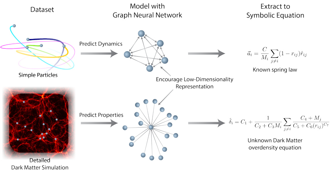
Figure 1: A cartoon depicting how we extract physical equations from a dataset.
图 1: 描述如何从数据集中提取物理方程的示意图。
Furthermore, generalization is difficult without prior knowledge about the data imposed directly on the model. Even if we impose strong inductive biases on the models to improve generalization, the learned parts of networks typically are linear piece-wise approximations which extrapolate linearly (if using ReLU as activation [3]).
此外,若缺乏直接施加于模型的数据先验知识,泛化将变得困难。即便我们通过强归纳偏置来提升模型的泛化能力,网络学习到的部分通常仍是线性分段近似,会以线性方式外推(若使用ReLU作为激活函数 [3])。
Here, we propose a general framework to leverage the advantages of both deep learning and symbolic regression. As an example, we study Graph Networks (GNs or GNNs) [4] as they have strong and well-motivated inductive biases that are very well suited to problems we are interested in. Then we apply symbolic regression to fit different internal parts of the learned model that operate on reduced size representations. The symbolic expressions can then be joined together, giving rise to an overall algebraic equation equivalent to the trained GN. Our work is a generalized and extended version of that in [5].
在此,我们提出一个通用框架,以结合深度学习和符号回归的优势。以图网络 (GNs或GNNs) [4] 为例,因其具有强大且合理的归纳偏置,非常适合我们感兴趣的问题。接着,我们应用符号回归来拟合学习模型中处理降维表示的不同内部部分。这些符号表达式随后可以组合起来,形成一个与训练好的图网络等效的整体代数方程。我们的工作是文献[5]中方法的广义扩展版本。
We apply our framework to three problems—rediscovering force laws, rediscovering Hamiltonians, and a real world astrophysical challenge—and demonstrate that we can drastically improve generalization, and distill plausible analytical expressions. We not only recover the injected closedform physical laws for Newtonian and Hamiltonian examples, we also derive a new interpret able closed-form analytical expression that can be useful in astrophysics.
我们将框架应用于三个问题——重新发现力定律、重新发现哈密顿量以及一个真实的天体物理学挑战——并证明我们能够显著提升泛化能力,同时提炼出合理的解析表达式。我们不仅复原了牛顿力学和哈密顿力学示例中预设的闭合形式物理定律,还推导出一个新的可解释闭合形式解析表达式,该表达式在天体物理学中可能具有实用价值。
2 Framework
2 框架
Our framework can be summarized as follows. (1) Engineer a deep learning model with a separable internal structure that provides an inductive bias well matched to the nature of the data. Specifically, in the case of interacting particles, we use Graph Networks as the core inductive bias in our models. (2) Train the model end-to-end using available data. (3) Fit symbolic expressions to the distinct functions learned by the model internally. (4) Replace these functions in the deep model by the symbolic expressions. This procedure with the potential to discover new symbolic expressions for non-trivial datasets is illustrated in fig. 1.
我们的框架可总结如下:(1) 设计一个具有可分离内部结构的深度学习模型,其归纳偏置与数据特性高度匹配。具体而言,在处理相互作用粒子时,我们采用图网络 (Graph Networks) 作为模型的核心归纳偏置。(2) 利用现有数据对模型进行端到端训练。(3) 为模型内部学得的各独立函数拟合符号表达式。(4) 用这些符号表达式替换深度模型中的对应函数。图1展示了这一流程,该方法有望为复杂数据集发现新的符号表达式。
Particle systems and Graph Networks. In this paper we focus on problems that can be well described as interacting particle systems. Nearly all of the physics we experience in our day-to-day life can be described in terms of interactions rules between particles or entities, so this is broadly relevant. Recent work has leveraged the inductive biases of Interaction Networks (INs) [6] in their generalized form, the Graph Network, a type of Graph Neural Network [7, 8, 9], to learn models of particle systems in many physical domains [6, 10, 11, 12, 13, 14, 15, 16].
粒子系统与图网络。本文主要研究可被良好描述为相互作用粒子系统的问题。我们日常生活中接触到的几乎所有物理现象都可以用粒子或实体间的相互作用规则来描述,因此这一研究具有广泛适用性。近期研究利用交互网络(INs) [6] 的广义形式——图网络(一种图神经网络 [7, 8, 9])的归纳偏置,在多个物理领域 [6, 10, 11, 12, 13, 14, 15, 16] 实现了粒子系统建模。
Therefore we use Graph Networks (GNs) at the core of our models, and incorporate into them physically motivated inductive biases appropriate for each of our case studies. Some other interesting approaches for learning low-dimensional general dynamical models include [17, 18, 19]. Other related work which studies the physical reasoning abilities of deep models include [20, 21, 22, 23].
因此,我们在模型核心采用了图网络 (Graph Networks, GNs),并针对每个案例研究融入了具有物理动机的归纳偏置。其他一些学习低维通用动力学模型的有趣方法包括 [17, 18, 19]。关于深度模型物理推理能力的其他相关研究包括 [20, 21, 22, 23]。
Internally, GNs are structured into three distinct components: an edge model, a node model, and a global model, which take on different but explicit roles in a regression problem. The edge model, or “message function,” which we denote by $\phi^{e}$ , maps from a pair of nodes $\mathbf{\dot{\Gamma}}(\mathbf{v}_ {i},\mathbf{v}_ {j}\in\mathbb{R}^{L_{v}}$ ) connected by an edge in a graph together with some vector information for the edge, to a message vector. These message vectors are summed element-wise for each receiving node over all of their sending nodes, and the summed vector is passed to the node model. The node model, $\phi^{v}$ , takes the receiving node and the summed message vector, and computes an updated node: a vector representing some property or dynamical update. Finally, a global model $\phi^{u}$ aggregates all messages and all updated nodes and computes a global property. $\phi^{e}$ , $\phi^{v}$ , $\phi^{u}$ are usually approximated using multilayer-perce ptr on s, making them differentiable end-to-end. More details on GNs are given in the appendix. We illustrate the internal structure of a GN in fig. 2.
在内部,图网络 (GN) 由三个独立组件构成:边模型 (edge model)、节点模型 (node model) 和全局模型 (global model),它们在回归问题中承担不同但明确的角色。边模型(或称“消息函数”),记为 $\phi^{e}$,将从图中通过边连接的一对节点 $\mathbf{\dot{\Gamma}}(\mathbf{v}_ {i},\mathbf{v}_ {j}\in\mathbb{R}^{L_{v}}$) 连同该边的某些向量信息,映射为一个消息向量。这些消息向量会按元素求和,针对每个接收节点,汇总其所有发送节点的消息,并将求和后的向量传递给节点模型。节点模型 $\phi^{v}$ 接收该节点和求和后的消息向量,并计算出一个更新后的节点:即表示某种属性或动态更新的向量。最后,全局模型 $\phi^{u}$ 汇总所有消息和所有更新后的节点,并计算出一个全局属性。$\phi^{e}$、$\phi^{v}$、$\phi^{u}$ 通常使用多层感知机 (multilayer perceptron) 进行近似,从而使它们可端到端微分。关于 GN 的更多细节见附录。我们在图 2 中展示了 GN 的内部结构。
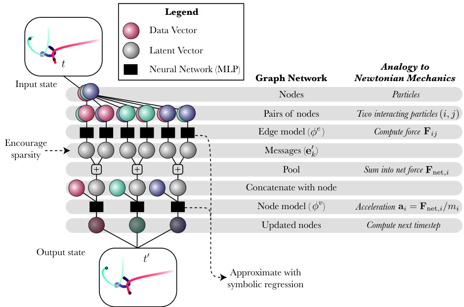
Figure 2: An illustration of the internal structure of the graph neural network we use in some of our experiments. Note that the comparison to Newtonian mechanics is purely for explanatory purposes, but is not explicit. Differences include: the “forces” (messages) are often high dimensional, the nodes need not be physical particles, $\phi^{e}$ and $\phi^{v}$ are arbitrary learned functions, and the output need not be an updated state. However, the rough equivalency between this architecture and physical frameworks allows us to interpret learned formulas in terms of existing physics.
图 2: 我们部分实验所用图神经网络内部结构示意图。需注意:与牛顿力学的类比仅出于解释目的,并非显式对应。差异包括:(1) "力"(消息)通常为高维向量 (2) 节点不必是物理粒子 (3) $\phi^{e}$ 和 $\phi^{v}$ 为任意学习函数 (4) 输出不一定是更新状态。但该架构与物理框架的粗略等效性,使我们能够用现有物理解释学习得到的公式。
GNs are the ideal candidate for our approach due to their inductive biases shared by many physics problems. (a) They are e qui variant under particle permutations. (b) They are differentiable end-to-end and can be trained efficiently using gradient descent. (c) They make use of three separate and interpret able internal functions $\phi^{e}$ , $\phi^{v}$ , $\phi^{u}$ , which are our targets for the symbolic regression. GNs can also be embedded with additional symmetries as in [24, 25], but we do not implement these.
由于图网络 (GNs) 的归纳偏置与许多物理问题相通,因此成为我们方法的理想选择:(a) 它们在粒子置换下具有等变性;(b) 可端到端微分,并能通过梯度下降高效训练;(c) 采用三个独立且可解释的内部函数 $\phi^{e}$、$\phi^{v}$、$\phi^{u}$ 作为符号回归的目标。虽然如 [24, 25] 所述可嵌入额外对称性,但本文未实现该功能。
Symbolic regression. After training the Graph Networks, we use the symbolic regression package eureqa [2] to perform symbolic regression and fit compact closed-form analytical expressions to $\phi^{e},\phi^{v}$ , and $\phi^{u}$ independently. eureqa works by using a genetic algorithm to combine algebraic expressions stochastic ally. The technique is similar to natural selection, where the “fitness” of each expression is defined in terms of simplicity and accuracy. The operators considered in the fitting process are $+,-,\times,/,>,<,\land$ , exp, log, $\operatorname{IF}(\cdot,\cdot,\cdot)$ as well as real constants. After fitting expressions to each part of the graph network, we substitute the expressions into the model to create an alternative analytic model. We then refit any parameters in the symbolic model to the data a second time, to avoid the accumulated approximation error. Further details are given in the appendix.
符号回归。训练完图网络后,我们使用符号回归工具包eureqa [2]对$\phi^{e}$、$\phi^{v}$和$\phi^{u}$分别进行符号回归,并拟合紧凑的闭式解析表达式。eureqa通过遗传算法随机组合代数表达式来实现这一过程,其原理类似于自然选择——每个表达式的"适应度"由简洁性和准确性共同定义。拟合过程中考虑的运算符包括$+,-,\times,/,>,<,\land$、exp、log、$\operatorname{IF}(\cdot,\cdot,\cdot)$以及实数常量。在为图网络的每个部分拟合表达式后,我们将这些表达式代入模型以创建替代的解析模型。为避免累积近似误差,我们会二次拟合符号模型中的所有参数。更多细节见附录。
This approach gives us an explicit way of interpreting the trained weights of a structured neural network. An alternative way of interpreting GNNs is given in [26]. This new technique also allows us to extend symbolic regression to high-dimensional datasets, where it is otherwise intractable. As an example, consider attempting to discover the relationship between a scalar and a time series, given data 
, where $z_{i}\in\mathbb{R}$ and $\mathbf{x}_ {i,j}\in\mathbb{R}^{5}$ . Assume the true relationship as $z_{i}=y_{i}^{2}$ , for $\begin{array}{r}{y_{i}=\sum_{j=1}^{100}y_{i,j}}\end{array}$ , $y_{i,j}=\exp(x_{i,j,3})+\cos(2x_{i,j,1})$ . Now, in a learnable model, assume an inductive bias $\begin{array}{r}{z_{i}=f(\sum_{j=1}^{100}g(\mathbf x_{i,j}))}\end{array}$ for scalar functions $f$ and $g$ . If we need to consider $10^{9}$ equations for both $f$ and $g$ , then a standard symbolic regression search would need to consider their combination, leading to $(\breve{10}^{9})^{2}=10^{18}$ equations in total. But if we first fit a neural network for $f$ and $g$ , and after training, fit an equation to $f$ and $g$ separately, we only need to consider $2\times10^{9}$ equations. In effect, we factorize high-dimensional datasets into smaller sub-problems that are tractable for symbolic regression.
该方法为我们提供了一种明确解释结构化神经网络训练权重的方式。[26]中给出了另一种解释图神经网络(GNN)的方法。这项新技术还使我们能够将符号回归扩展到高维数据集,而传统方法对此类问题难以处理。例如,给定数据集
(其中$z_{i}\in\mathbb{R}$,$\mathbf{x}_ {i,j}\in\mathbb{R}^{5}$),假设真实关系为$z_{i}=y_{i}^{2}$,其中$\begin{array}{r}{y_{i}=\sum_{j=1}^{100}y_{i,j}}\end{array}$,$y_{i,j}=\exp(x_{i,j,3})+\cos(2x_{i,j,1})$。在一个可学习模型中,若采用归纳偏置$\begin{array}{r}{z_{i}=f(\sum_{j=1}^{100}g(\mathbf x_{i,j}))}\end{array}$(标量函数$f$和$g$),当需要为$f$和$g$各考虑$10^{9}$个方程时,标准符号回归搜索需要处理它们的组合情况,总计达$(\breve{10}^{9})^{2}=10^{18}$个方程。但如果我们先为$f$和$g$拟合神经网络,训练完成后分别对$f$和$g$进行方程拟合,则只需考虑$2\times10^{9}$个方程。这种方法本质上将高维数据集分解为符号回归可处理的更小子问题。
We emphasize that this method is not a new symbolic regression technique by itself; rather, it is a way of extending any existing symbolic regression method to high-dimensional datasets by the use of a neural network with a well-motivated inductive bias. While we chose eureqa for our experiments based on its efficiency and ease-of-use, we could have chosen another low-dimensional symbolic regression package, such as our new high-performance package $P y S R^{1}$ [27]. Other community packages such as [28, 29, 30, 31, 32, 33, 34, 35, 36], could likely also be used and achieve similar results (although [32] is unable to fit the constants required for the tasks here). Ref. [29] is an interesting approach that uses gradient descent on a pre-defined equation up to some depth, para met rize d with a neural network, instead of genetic algorithms; [35] uses gradient descent on a latent embedding of an equation; and [36] demonstrates Monte Carlo Tree Search as a symbolic regression technique, using an asymptotic constraint as input to a neural network which guides the search. These could all be used as drop-in replacements for eureqa here to extend their algorithms to high-dimensional datasets.
我们强调,该方法本身并非新的符号回归技术,而是通过使用具有合理归纳偏置的神经网络,将现有任何符号回归方法扩展到高维数据集的一种途径。虽然我们基于效率和易用性选择了eureqa进行实验,但也可以选用其他低维符号回归工具包,例如我们新的高性能工具包$PySR^{1}$[27]。其他社区工具包如[28, 29, 30, 31, 32, 33, 34, 35, 36]可能同样适用并取得类似效果(尽管[32]无法拟合当前任务所需的常数)。文献[29]提出了一种有趣的方法,在预定义方程上执行梯度下降至特定深度,通过神经网络进行参数化,而非遗传算法;[35]在方程的潜在嵌入空间执行梯度下降;[36]则展示了将蒙特卡洛树搜索作为符号回归技术,使用渐近约束作为神经网络的搜索引导输入。这些方法均可作为eureqa的即插即用替代方案,将其算法扩展至高维数据集。
We also note several exciting packages for symbolic regression of partial differential equations on gridded data: [37, 38, 39, 40, 41, 42]. These either use sparse regression of coefficients over a library of PDE terms, or a genetic algorithm. While not applicable to our use-cases, these would be interesting to consider for future extensions to gridded PDE data.
我们还注意到几个针对网格数据偏微分方程符号回归的激动人心的工具包:[37, 38, 39, 40, 41, 42]。这些工具包要么通过对偏微分方程项库进行系数稀疏回归,要么采用遗传算法。虽然不适用于我们的使用场景,但对于未来扩展到网格偏微分方程数据的研究值得关注。
Compact internal representations. While training, we encourage the model to use compact internal representations for latent hidden features (e.g., messages) by adding regular iz ation terms to the loss (we investigate using $\mathrm{L_{1}}$ and KL penalty terms with a fixed prior, see more details in the Appendix). One motivation for doing this is based on Occam’s Razor: science always prefers the simpler model or representation of two which give similar accuracy. Another stronger motivation is that if there is a law that perfectly describes a system in terms of summed message vectors in a compact space (what we call a linear latent space), then we expect that a trained GN, with message vectors of the same dimension as that latent space, will be mathematical rotations of the true vectors. We give a mathematical explanation of this reasoning in the appendix, and emphasize that while it may seem obvious now, our work is the first to demonstrate it. More practically, by reducing the size of the latent representations, we can filter out all low-variance latent features without compromising the accuracy of the model, and vastly reducing the dimensionality of the hidden vectors. This makes the symbolic regression of the internal models more tractable.
紧凑的内部表征。在训练过程中,我们通过在损失函数中添加正则化项(研究了使用$\mathrm{L_{1}}$和基于固定先验的KL惩罚项,详见附录),鼓励模型对潜在隐藏特征(如消息)采用紧凑的内部表征。这一做法的动机之一源于奥卡姆剃刀原则:在精度相近的情况下,科学总是倾向于选择更简单的模型或表征方式。另一个更重要的动机是,如果存在某个定律能用紧凑空间(我们称为线性潜空间)中的消息向量之和完美描述系统,那么经过训练的GN(其消息向量维度与该潜空间相同)所生成的向量,理论上应是真实向量的数学旋转。我们在附录中给出了该推论的数学解释,并强调尽管现在看起来显而易见,但我们的工作首次实证了这一观点。从实用角度而言,通过缩小潜在表征的尺寸,我们可以在不影响模型精度的前提下过滤所有低方差潜在特征,从而大幅降低隐藏向量的维度。这使得内部模型的符号回归更易处理。
Implementation details. We write our models with PyTorch [43] and PyTorch Geometric[44]. We train them with a decaying learning schedule using Adam [45]. The symbolic regression technique is described in section 4.1. More details are provided in the Appendix.
实现细节。我们使用PyTorch [43]和PyTorch Geometric[44]编写模型,采用Adam优化器[45]配合衰减学习率进行训练。符号回归技术详见第4.1节,更多细节参见附录。
3 Case studies
3 案例研究
In this section we present three specific case studies where we apply our proposed framework using additional inductive biases.
在本节中,我们将通过三个具体案例研究展示如何运用额外归纳偏置来实施所提出的框架。
Newtonian dynamics. Newtonian dynamics describes the dynamics of particles according to Newton’s law of motion: the motion of each particle is modeled using incident forces from nearby particles, which change its position, velocity and acceleration. Many important forces in physics (e.g., gravitational force $-{\frac{G m_{1}m_{2}}{r^{2}}}{\hat{r}})$ are defined on pairs of particles, analogous to the message function $\phi^{e}$ of our Graph Networks. The summation that aggregates messages is analogous to the calculation of the net force on a receiving particle. Finally, the node function, $\phi^{v}$ , acts like Newton’s law: acceleration equals the net force (the summed message) divided by the mass of the receiving particle.
牛顿动力学。牛顿动力学根据牛顿运动定律描述粒子的运动规律:每个粒子的运动通过附近粒子施加的作用力来建模,这些力会改变其位置、速度和加速度。物理学中许多重要力(如引力 $-{\frac{G m_{1}m_{2}}{r^{2}}}{\hat{r}})$ 都是在粒子对之间定义的,类似于我们图网络中的消息函数 $\phi^{e}$。聚合消息的求和运算类似于计算接收粒子的净受力。最后,节点函数 $\phi^{v}$ 的作用类似于牛顿定律:加速度等于净受力(即聚合后的消息)除以接收粒子的质量。
To train a model on Newtonian dynamics data, we train the GN to predict the instantaneous acceleration of the particle against that calculated in the simulation. While Newtonian mechanics inspired the original development of INs, never before has an attempt to distill the relationship between the forces and the learned messages been successful. When applying the framework to this Newtonian dynamics problem (as illustrated in fig. 1), we expect the model trained with our framework to discover that the optimal dimensionality of messages should match the number of spatial dimensions. We also expect to recover algebraic formulas for pairwise interactions, and generalize better than purely learned models. We refer our readers to section 4.1 and the Appendix for more details.
为了在牛顿动力学数据上训练模型,我们训练GN(Graph Network)来预测粒子瞬时加速度与模拟计算值的差异。虽然牛顿力学启发了INs(Interaction Networks)的原始开发,但此前从未成功提炼出作用力与学习消息之间的关联关系。将该框架应用于牛顿动力学问题时(如图1所示),我们预期采用本框架训练的模型将发现:消息的最优维度应与空间维度数相匹配。同时有望恢复出成对相互作用的代数公式,并展现出比纯学习模型更优的泛化能力。更多细节详见第4.1节与附录。
Hamiltonian dynamics. Hamiltonian dynamics describes a system’s total energy $\mathcal{H}(\mathbf{q},\mathbf{p})$ as a function of its canonical coordinates q and momenta p—e.g., each particle’s position and momentum. The dynamics of the system change perpendicular ly to the gradient of $\mathcal{H}$ : $\begin{array}{r}{\frac{\mathrm{d}\mathbf{\bar{q}}}{\mathrm{d}t}=\frac{\partial\mathcal{H}}{\partial\mathbf{p}}}\end{array}$ , $\begin{array}{r}{\frac{\mathrm{d}\mathbf{p}}{\mathrm{d}t}=-\frac{\mathrm{d}\mathcal{H}}{\mathrm{d}\mathbf{q}}}\end{array}$ .
哈密顿动力学。哈密顿动力学将系统的总能量 $\mathcal{H}(\mathbf{q},\mathbf{p})$ 描述为其正则坐标 q 和动量 p 的函数(例如每个粒子的位置和动量)。系统动态沿 $\mathcal{H}$ 梯度的垂直方向变化:$\begin{array}{r}{\frac{\mathrm{d}\mathbf{\bar{q}}}{\mathrm{d}t}=\frac{\partial\mathcal{H}}{\partial\mathbf{p}}}\end{array}$,$\begin{array}{r}{\frac{\mathrm{d}\mathbf{p}}{\mathrm{d}t}=-\frac{\mathrm{d}\mathcal{H}}{\mathrm{d}\mathbf{q}}}\end{array}$。
Here, we will use a variant of a Hamiltonian Graph Network (HGN) [46] to learn $\mathcal{H}$ for the Newtonian dynamics data. This model is a combination of a Hamiltonian Neural Network [47, 48] and GN. In this case, the global model $\phi^{u}$ of the GN will output a single scalar value for the entire system representing the energy, and hence the GN will have the same functional form as a Hamiltonian. By then taking the partial derivatives of the GN-predicted $\mathcal{H}$ with respect to the position and momentum, q and p, respectively, of the input nodes, we will be able to calculate the updates to the momentum and position. We impose a modification to the HGN to facilitate its interpret ability, and name this the “Flattened HGN” or FlatHGN: instead of summing high-dimensional encodings of nodes to calculate $\phi^{u}$ , we instead set it to be a sum of scalar pairwise interaction terms, ${\mathcal{H}}_ {\mathrm{pair}}$ and a per-particle term, $\mathcal{H}_{\mathrm{self}}$ . This is because many physical systems can be exactly described this way. This is a Hamiltonian version of the Lagrangian Graph Network in [49], and is similar to [50]. This is still general enough to express many physical systems, as nearly all of physics can be written as summed interaction energies, but could also be relaxed in the context of the framework.
此处我们将采用哈密顿图网络 (HGN) [46] 的变体来学习牛顿动力学数据中的 $\mathcal{H}$。该模型结合了哈密顿神经网络 [47, 48] 和图网络 (GN)。在此架构中,图网络的全局模型 $\phi^{u}$ 会输出代表系统总能量的标量值,从而使图网络具备与哈密顿量相同的函数形式。通过对图网络预测的 $\mathcal{H}$ 分别求输入节点位置 (q) 和动量 (p) 的偏导数,即可计算动量和位置的更新量。为提升模型可解释性,我们对 HGN 进行了改进并命名为"扁平化 HGN"(FlatHGN):不再通过节点高维编码求和来计算 $\phi^{u}$,而是将其设置为标量对相互作用项 ${\mathcal{H}}_ {\mathrm{pair}}$ 与单粒子项 $\mathcal{H}_{\mathrm{self}}$ 之和。这种设计源于许多物理系统都可采用此方式精确描述的特性。该模型是文献 [49] 中拉格朗日图网络的哈密顿版本,其原理与文献 [50] 相似。这种架构仍具有足够普适性来表达多数物理系统(因几乎所有物理现象都可表述为相互作用能量之和),但也可在该框架下进行灵活调整。
Even though the model is trained end-to-end, we expect our framework to allow us to extract analytical expressions for both the per-particle kinetic energy, and the scalar pairwise potential energy. We refer our readers to our section 4.2 and the Appendix for more details.
尽管该模型是端到端训练的,但我们期望该框架能让我们提取出单粒子动能和标量成对势能的解析表达式。更多细节请参阅第4.2节和附录部分。
Dark matter halos for cosmology. We also apply our framework to a dataset generated from stateof-the-art dark matter simulations [51]. We predict a property (“over density”) of a dark matter blob (called a “halo”) from the properties (positions, velocities, masses) of halos nearby. We would like to extract this relationship as an analytic expression so we may interpret it theoretically. This problem differs from the previous two use cases in many ways, including (1) it is a real-world problem where an exact analytical expression is unknown; (2) the problem does not involve dynamics, rather, it is a regression problem on a static dataset; and (3) the dataset is not made of particles, but rather a grid of density that has been grouped and reduced to handmade features. Similarly, we do not know the dimensionality of interactions, should a linear latent space exist. We rely on our inductive bias to find the optimal dimensional of the problem, and then yield an interpret able model that performs better than existing analytical approximations. We refer our readers to our section 4.3 and the Appendix for further details.
宇宙学中的暗物质晕。我们还将该框架应用于由最先进的暗物质模拟[51]生成的数据集。我们通过附近暗物质晕的属性(位置、速度、质量)来预测暗物质团块(称为"晕")的一个属性("过密度")。我们希望将此关系提取为解析表达式以便进行理论解释。该问题与前两个应用场景存在多方面差异:(1) 这是一个真实世界问题,其精确解析表达式未知;(2) 问题不涉及动力学,而是针对静态数据集的回归问题;(3) 数据集并非由粒子构成,而是经过分组和特征工程处理的密度网格数据。同样地,即便存在线性潜空间,我们也无法预知相互作用的维度。我们依靠归纳偏置来寻找问题的最优维度,最终获得性能优于现有解析近似方法且可解释的模型。更多细节请参阅第4.3节和附录部分。
4 Experiments & results
4 实验与结果
4.1 Newtonian dynamics
4.1 牛顿动力学
We train our Newtonian dynamics GNs on data for simple N-body systems with known force laws. We then apply our technique to recover the known force laws via the representations learned by the message function $\phi^{e}$ .
我们在已知作用力定律的简单N体系统数据上训练牛顿动力学图网络 (GN)。随后运用该方法,通过消息函数 $\phi^{e}$ 学习到的表征来恢复已知的作用力定律。
Data. The dataset consists of N-body particle simulations in two and three dimensions, under different interaction laws. We used the following forces: (a) $1/r$ orbital force: $-m_{1}m_{2}\hat{r}/r$ ; (b) $1/r^{2}$ orbital force $-m_{1}m_{2}\hat{r}/r^{2}$ ; (c) charged particles force $q_{1}q_{2}\hat{r}/r^{2}$ ; (d) damped springs with $\left|r-1\right|^{2}$ potential and damping proportional and opposite to speed; (e) discontinuous forces, $-{0,r^{2}}r$ , switching to 0 force for $r:<2:$ ; and (f) springs between all particles, a $(r-1)^{2}$ potential. The simulations themselves contain masses and charges of 4 or 8 particles, with positions, velocities, and accelerations as a function of time. Further details of these systems are given in the appendix, with example trajectories shown in fig. 4.
数据。该数据集包含二维和三维空间中遵循不同相互作用规律的N体粒子模拟。我们采用了以下作用力:(a) $1/r$ 轨道力:$-m_{1}m_{2}\hat{r}/r$;(b) $1/r^{2}$ 轨道力 $-m_{1}m_{2}\hat{r}/r^{2}$;(c) 带电粒子间作用力 $q_{1}q_{2}\hat{r}/r^{2}$;(d) 阻尼弹簧系统,其势能为 $\left|r-1\right|^{2}$ 且阻尼力与速度大小成正比、方向相反;(e) 不连续作用力 $-{0,r^{2}}r$,当 $r:<2:$ 时作用力切换为0;(f) 全粒子间弹簧系统,其势能为 $(r-1)^{2}$。模拟对象为4或8个具有质量与电荷的粒子,其位置、速度和加速度均为时间的函数。这些系统的详细说明见附录,示例轨迹如fig. 4所示。
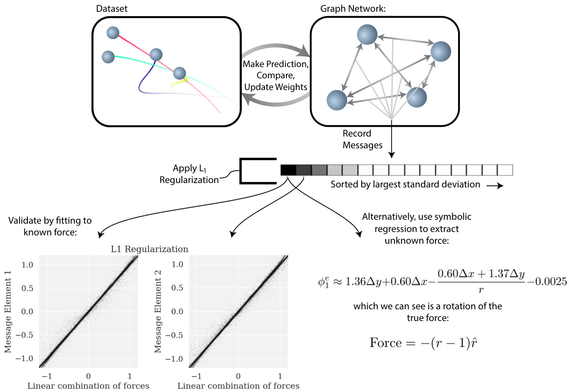
Figure 3: A diagram showing how we implement and exploit our inductive bias on GNs. A video of this figure during training can be seen by going to the URL https://github.com/Miles Cranmer/ symbolic deep learning/blob/master/video_link.txt.
图 3: 展示如何在图网络(GNs)上实现并利用归纳偏置的示意图。训练过程中该图的动态演示视频可通过访问 URL https://github.com/MilesCranmer/symbolic-deep-learning/blob/master/video_link.txt 观看。
Model training. The models are trained to predict instantaneous acceleration for every particle given the current state of the system. To investigate the importance of the size of the message representations for interpreting the messages as forces, we train our GN using 4 different strategies: 1. Standard, a GN with 100 message components; 2. Bottleneck, a GN with the number of message components matching the dimensionality of the problem (2 or 3); 3. $\mathrm{L_{1}}$ , same as “Standard” but using a $\mathrm{L_{1}}$ regular iz ation loss term on the messages with a weight of $10^{-2}$ ; and 4. KL same as “Standard” but regularizing the messages using the Kullback-Leibler (KL) divergence with respect to Gaussian prior. Both the $\mathrm{L_{1}}$ and KL strategies encourage the network to find compact representations for the message vectors, using different regular iz at ions. We optimize the mean absolute loss between the predicted acceleration and the true acceleration of each node. Additional training details are given in the appendix and found in the codebase.
模型训练。这些模型被训练用于根据系统的当前状态预测每个粒子的瞬时加速度。为了研究消息表示大小对将消息解释为力的重要性,我们采用4种不同策略训练图网络(GN):1. 标准模式,使用100个消息组件的GN;2. 瓶颈模式,消息组件数量与问题维度(2或3)匹配的GN;3. $\mathrm{L_{1}}$ 模式,与"标准"相同但对消息施加权重为 $10^{-2}$ 的 $\mathrm{L_{1}}$ 正则化损失项;4. KL模式,与"标准"相同但使用Kullback-Leibler (KL)散度对消息进行高斯先验正则化。$\mathrm{L_{1}}$ 和KL策略都通过不同正则化方式促使网络寻找消息向量的紧凑表示。我们优化每个节点预测加速度与真实加速度之间的平均绝对损失。更多训练细节见附录和代码库。
Performance comparison. To evaluate the learned models, we generate a new dataset from a different random seed. We find that the model with $\mathrm{L_{1}}$ regular iz ation has the greatest prediction performance in most cases (see table 3). It is worth noting that the bottleneck model, even though it has the correct dimensional ty, performs worse than the model using $\mathrm{L_{1}}$ regular iz ation under limited training time. We speculate that this may connect to the lottery ticket hypothesis [52].
性能对比。为评估学习到的模型,我们使用不同随机种子生成新数据集。发现采用 $\mathrm{L_{1}}$ 正则化的模型在多数情况下预测性能最佳(见表3)。值得注意的是,即使瓶颈模型具有正确维度,在有限训练时长下其表现仍逊于采用 $\mathrm{L_{1}}$ 正则化的模型。我们推测这可能与彩票假设[52]有关。
Interpreting the message components. As a first attempt to interpret the information in the message components, we pick the $D$ message features (where $D$ is the dimensionality of the simulation) with the highest variance (or KL divergence), and fit each to a linear combination of the true force components. We find that while the GN trained in the Standard setting does not show strong correlations with force components (also seen in fig. 5), all other models for which the effective message size is constrained explicitly (bottleneck) or implicitly (KL or $\mathrm{L_{1}}$ ) to be low dimensional yield messages that are highly correlated with the true forces (see table 1 which indicates the fit errors with respect to the true forces), with the model trained with $\mathrm{L_{1}}$ regular iz ation showing the highest correlations. An explicit demonstration that the messages in a graph network learn forces has not been observed before our work.
解析消息组件。作为初步尝试,我们选取方差(或KL散度)最大的$D$个消息特征($D$为模拟维度),将其拟合为真实力分量的线性组合。研究发现:标准训练设置的图网络(GN)与力分量未呈现强相关性(图5亦可见),而所有通过显式(瓶颈层)或隐式(KL/$\mathrm{L_{1}}$)约束将有效消息维度限制为低维的模型,其生成消息均与真实力高度相关(见表1中拟合误差指标)。其中采用$\mathrm{L_{1}}$正则化训练的模型展现出最高相关性。图网络消息学习力学规律的现象,在我们的工作之前尚未被明确揭示。
The messages in these models are thus explicitly interpret able as forces. The video at https://github.com/Miles Cranmer/symbolic deep learning/blob/master/video_ link.txt (fig. 3) shows a fit of the message components over time during training, showing how the model discovers a message representation that is highly correlated with a rotation of the true force vector in an unsupervised way.
这些模型中的消息因此可明确解释为力。视频链接 https://github.com/Miles Cranmer/symbolic-deep-learning/blob/master/video_link.txt (图 3) 展示了训练过程中消息组件随时间变化的拟合情况,显示了模型如何以无监督方式发现与真实力向量旋转高度相关的消息表示。
| Sim. | Standard | Bottleneck | L1 | KL |
| Charge-2 | 0.016 | 0.947 | 0.004 | 0.185 |
| Charge-3 | 0.013 | 0.980 | 0.002 | 0.425 |
| r-1-2 | 0.000 | 1.000 | 1.000 | 0.796 |
| r-1-3 | 0.000 | 1.000 | 1.000 | 0.332 |
| r-2-2 | 0.004 | 0.993 | 0.990 | 0.770 |
| r-2-3 | 0.002 | 0.994 | 0.977 | 0.214 |
| Spring-2 | 0.032 | 1.000 | 1.000 | 0.883 |
| Spring-3 | 0.036 | 0.995 | 1.000 | 0.214 |
| Sim. | Standard | Bottleneck | L1 | KL |
|---|---|---|---|---|
| Charge-2 | 0.016 | 0.947 | 0.004 | 0.185 |
| Charge-3 | 0.013 | 0.980 | 0.002 | 0.425 |
| r-1-2 | 0.000 | 1.000 | 1.000 | 0.796 |
| r-1-3 | 0.000 | 1.000 | 1.000 | 0.332 |
| r-2-2 | 0.004 | 0.993 | 0.990 | 0.770 |
| r-2-3 | 0.002 | 0.994 | 0.977 | 0.214 |
| Spring-2 | 0.032 | 1.000 | 1.000 | 0.883 |
| Spring-3 | 0.036 | 0.995 | 1.000 | 0.214 |
Table 1: The $R^{2}$ value of a fit of a linear combination of true force components to the message components for a given model (see text). Numbers close to 1 indicate the messages and true force are strongly correlated. Successes/failures of force law symbolic regression are tabled in the appendix.
表 1: 给定模型中真实力分量线性组合与消息分量拟合的 $R^{2}$ 值 (详见正文)。接近1的数值表明消息与真实力高度相关。力定律符号回归的成功/失败案例列于附录中。
Symbolic regression on the internal functions. We now demonstrate symbolic regression to extract force laws from the messages, without using prior knowledge for each force’s form. To do this, we record the most significant message component of $\phi^{e}$ , which we refer to as $\phi_{1}^{e}$ , over random samples of the training dataset. The inputs to the regression are $m_{1},m_{2},q_{1},q_{2},x_{1},x_{2},...$ (mass, charge, $\mathbf{X}$ -position of receiving and sending node) as well as simplified variables to help the symbolic regression: e.g., $\Delta x$ for $x$ displacement, and $r$ for distance.
内部函数的符号回归。我们现在演示如何通过符号回归从消息中提取力定律,而无需预先了解每种力的形式。为此,我们在训练数据集的随机样本中记录 $\phi^{e}$ 的最显著消息分量 $\phi_{1}^{e}$。回归的输入包括 $m_{1},m_{2},q_{1},q_{2},x_{1},x_{2},...$(质量、电荷、接收与发送节点的 $\mathbf{X}$ 坐标)以及用于辅助符号回归的简化变量:例如位移 $\Delta x$ 和距离 $r$。
We then use eureqa to fit the $\phi_{1}^{e}$ to the inputs by minimizing the mean absolute error (MAE) over various analytic functions. Analogous to Occam’s razor, we find the “best” algebraic model by asking eureqa to provide multiple candidate fits at different complexity levels (where complexity is scored as a function of the number and the type of operators, constants and input variables used), and select the fit that maximizes the fractional drop in mean absolute error (MAE) over the increase in complexity from the next best model: $(-\Delta\log(\mathrm{{\bar{M}A E}}_{c})/\Delta c)$ . From this, we recover many analytical expressions (this is tabled in the appendix) that are equivalent to the simulated force laws $(a,b$ indicate learned constants):
我们随后利用eureqa,通过最小化不同解析函数的平均绝对误差(MAE)来拟合$\phi_{1}^{e}$的输入参数。类似于奥卡姆剃刀原则,我们通过要求eureqa提供不同复杂度层级(复杂度评分基于所用运算符、常数和输入变量的数量与类型)的多个候选拟合方案,并选择使平均绝对误差(MAE)分数下降与复杂度增幅比值$(-\Delta\log(\mathrm{{\bar{M}A E}}_{c})/\Delta c)$最大化的拟合结果,从而确定"最佳"代数模型。通过这种方法,我们还原出许多与模拟力定律等效的解析表达式(见附录表格),其中$(a,b$代表学习得到的常数):
• Spring, 2D, $\mathrm{L_{1}}$ (expect $\begin{array}{r}{\phi_{1}^{e}\approx(\mathbf{a}\cdot(\Delta x,\Delta y))(r-1)+b).}\end{array}$
• Spring, 2D, $\mathrm{L_{1}}$ (预期 $\begin{array}{r}{\phi_{1}^{e}\approx(\mathbf{a}\cdot(\Delta x,\Delta y))(r-1)+b).}\end{array}$
$$
\phi_{1}^{e}\approx1.36\Delta y+0.60\Delta x-\frac{0.60\Delta x+1.37\Delta y}{r}-0.0025
$$
$$
\phi_{1}^{e}\approx1.36\Delta y+0.60\Delta x-\frac{0.60\Delta x+1.37\Delta y}{r}-0.0025
$$
• $1/r^{2}$ , 3D, Bottleneck (expect $\begin{array}{r}{\phi_{1}^{e}\approx\frac{\mathbf{a}\cdot(\Delta x,\Delta y,\Delta z)}{r^{3}}+b)}\end{array}$ .
• $1/r^{2}$,3D,瓶颈(预期 $\begin{array}{r}{\phi_{1}^{e}\approx\frac{\mathbf{a}\cdot(\Delta x,\Delta y,\Delta z)}{r^{3}}+b)}\end{array}$)。
$$
\phi_{1}^{e}\approx\frac{0.021\Delta x m_{2}-0.077\Delta y m_{2}}{r^{3}}
$$
$$
\phi_{1}^{e}\approx\frac{0.021\Delta x m_{2}-0.077\Delta y m_{2}}{r^{3}}
$$
• Discontinuous, 2D, $\mathrm{L_{1}}$ (expect $\phi_{1}^{e}\approx\mathrm{IF}(r>2,(\mathbf{a}\cdot(\Delta x,\Delta y,\Delta z))r,0)+b).$
• 不连续,二维,$\mathrm{L_{1}}$(预期$\phi_{1}^{e}\approx\mathrm{IF}(r>2,(\mathbf{a}\cdot(\Delta x,\Delta y,\Delta z))r,0)+b)。
$$
\phi_{1}^{e}\approx\mathrm{{IF}}(r>2,0.15r\Delta y+0.19r\Delta x,0)-0.038
$$
$$
\phi_{1}^{e}\approx\mathrm{{IF}}(r>2,0.15r\Delta y+0.19r\Delta x,0)-0.038
$$
Note that reconstruction does not always succeed, especially for training strategies other than $\mathrm{L_{1}}$ or bottleneck models that cannot successfully find compact representations of the right dimensionality (see some examples in Appendix).
需要注意的是,重建并不总能成功,尤其是对于除 $\mathrm{L_{1}}$ 之外的训练策略,或是那些无法成功找到合适维度紧凑表示的瓶颈模型(参见附录中的部分示例)。
4.2 Hamiltonian dynamics
4.2 哈密顿动力学
Using the same datasets from the Newtonian dynamics case study, we also train our “FlatHGN,” with the Hamiltonian inductive bias, and demonstrate that we can extract scalar potential energies, rather than forces, for all of our problems. For example, in the case of charged particles, with expected potential $\begin{array}{r}{(\mathcal{H}_ {\mathrm{pair}}\approx\frac{a q_{1}q_{2}}{r})}\end{array}$ , symbolic regression applied to the learned message function yields2: Hpair ≈ 0.001r9q1q2 .
利用牛顿动力学案例研究中的相同数据集,我们还训练了具有哈密顿归纳偏置的"FlatHGN",并证明可以针对所有问题提取标量势能而非作用力。例如在带电粒子案例中,当预期势能为 $\begin{array}{r}{(\mathcal{H}_ {\mathrm{pair}}\approx\frac{a q_{1}q_{2}}{r})}\end{array}$ 时,对学习到的消息函数应用符号回归可得到2:Hpair ≈ 0.001r9q1q2。
It is also possible to fit the per-particle term $\mathcal{H}_ {\mathrm{self}}$ , however, in this case the same kinetic energy expression is recovered for all systems. In terms of performance results, the Hamiltonian models are comparable to that of the $\mathrm{L_{1}}$ regularized model across all datasets (See Supplementary results table).
同样可以拟合每个粒子的项 $\mathcal{H}_ {\mathrm{self}}$,但在这种情况下,所有系统都会恢复相同的动能表达式。从性能结果来看,哈密顿模型在所有数据集上与 $\mathrm{L_{1}}$ 正则化模型表现相当(参见补充结果表)。
Note that in this case, by design, the “FlatHGN“ has a message function with a dimensionality of 1 to match the output of the Hamiltonian function which is a scalar, so no regular iz ation is needed, as the message size is directly constrained to the right dimension.
请注意,在这种情况下,根据设计,"FlatHGN"的消息函数维度为1,以匹配哈密顿函数(Hamiltonian function)的标量输出,因此不需要正则化(regularization),因为消息大小直接被约束到正确的维度。
4.3 Dark matter halos for cosmology
4.3 宇宙学中的暗物质晕
Now, one may ask: “will this strategy also work for general regression problems, non-trivial datasets, complex interactions, and unknown laws?” Here we give an example that satisfies all four of these concerns, using data from a gravitational simulation of the Universe.
现在有人可能会问:"这种策略是否也适用于一般的回归问题、非平凡数据集、复杂交互和未知规律?"这里我们用一个满足所有这四个条件的例子,使用的是来自宇宙引力模拟的数据。
Cosmology studies the evolution of the Universe from the Big Bang to the complex galaxies and stars we see today [53]. The interactions of various types of matter and energy drive this evolution. Dark Matter alone consists of $\approx85%$ of the total matter in the Universe [54, 55], and therefore is extremely important for the development of galaxies. Dark matter particles clump together and act as gravitational basins called “halos” which pull regular baryonic matter together to produce stars, and form larger structures such as filaments and galaxies. It is an important question in cosmology to predict properties of dark matter halos based on their “environment,” which consist of other nearby dark matter halos. Here we study the following problem: how can we predict the excess amount of matter (in comparison to its surroundings, $\begin{array}{r}{\delta=\frac{\bar{\rho}-\langle\rho\rangle}{\langle\rho\rangle},}\end{array}$ ) for a dark matter halo based on its properties and those of its neighboring dark matter halos?
宇宙学研究宇宙从大爆炸到现今复杂星系与恒星的演化过程[53]。各类物质与能量的相互作用推动着这一演化。暗物质 (Dark Matter) 独占了宇宙总物质约85%[54,55],因此对星系的形成至关重要。暗物质粒子聚集成团,形成称为"晕"的引力势阱,吸引普通重子物质聚集形成恒星,并构建出纤维状结构及星系等更大尺度的结构。宇宙学中的一个关键问题是:如何根据暗物质晕所处的"环境"(即邻近其他暗物质晕)来预测其特性。本文研究以下问题:如何基于暗物质晕自身特性及其邻近暗物质晕的特性,预测该晕相对于周围环境的物质超额量 $\begin{array}{r}{\delta=\frac{\bar{\rho}-\langle\rho\rangle}{\langle\rho\rangle},}\end{array}$?
A hand-designed estimator for the functional form of $\delta_{i}$ for halo $i$ might correlate $\delta$ with the mass of the same halo, $M_{i}$ , as well as the mass within 20 distance units (we decide to use 20 as the smoothing radius): |j=ii− $\sum_{j\neq i}^{\left|\mathbf{r}_ {i}-\mathbf{r}_ {j}\right|<20}M_{j}$ . The intuition behind this scaling is described in [56]. Can we find a better equatio n that we can fit better to the data, using our methodology?
针对晕 $i$ 的函数形式 $\delta_{i}$ 手工设计的估计器,可能会将 $\delta$ 与同一晕的质量 $M_{i}$ 以及20个距离单位内的质量相关联(我们决定使用20作为平滑半径): |j=ii− $\sum_{j\neq i}^{\left|\mathbf{r}_ {i}-\mathbf{r}_ {j}\right|<20}M_{j}$。这种缩放背后的直觉在[56]中有描述。我们能否利用现有方法找到一个更优且更贴合数据的方程?
Data, training and symbolic regression. We study this problem with the open sourced N-body dark matter simulations from [51]. We choose the zeroth simulation in this dataset, at the final time step (current day Universe), which contains 215,854 dark matter halos. Each halo has mass $M_{i}$ , position $\mathbf{r}_ {i}$ , and velocity $\mathbf{v}_ {i}$ . We also compute the smoothed over density $\delta_{i}$ at the location of the center of each halo. We convert this set of halos into a graph by connecting halos within fifty distance units (each distance unit is approximately 3 million light years long) of each other. This results in 30,437,218 directional edges between halos, or 71 neighbors per halo on average. We then attempt to predict $\delta_{i}$ for each halo with a GN. Training details are the same as for the Newtonian simulations, but we switch to 500 hidden units after hyper parameter tuning based on GN accuracy.
数据、训练与符号回归。我们使用[51]中开源N体暗物质模拟研究该问题,选取该数据集中第零号模拟的最终时间步(当前宇宙状态),包含215,854个暗物质晕。每个晕具有质量$M_{i}$、位置$\mathbf{r}_ {i}$和速度$\mathbf{v}_ {i}$,同时计算了各晕中心位置的平滑密度$\delta_{i}$。通过连接彼此距离在50单位内(每单位约合300万光年)的晕,将其转换为图结构,最终形成30,437,218条有向边,平均每个晕拥有71个邻居节点。随后采用图网络(GN)预测各晕的$\delta_{i}$。训练参数与牛顿模拟实验相同,但基于GN精度超参数调优后隐层单元数调整为500。
The GN trained with $\mathrm{L_{1}}$ appears to have messages containing only 1 informative feature, so we extract message samples for this component of the messages over the training set for random pairs of halos, and node function samples for random receiving halos and their summed messages. The formula extracted by the algorithm is given in table 2 as “Best, with mass”. The form of the formula is new and it captures a well-known relationship between halo mass and environment: bias-mass relationship. We refit the parameters in the formula on the original training data to avoid accumulated approximation error from the multiple levels of function fitting. We achieve a loss of 0.0882 where the hand-designed formula achieves a loss of 0.121. It is quite surprising that our formula extracted by our approach is able to achieve a better fit than the formula hand-designed by scientists.
使用 $\mathrm{L_{1}}$ 训练的 GN (Graph Network) 生成的消息似乎仅包含1个信息特征,因此我们从训练集中随机选取成对晕族,提取消息中该组件的样本,并针对随机接收晕族及其汇总消息提取节点函数样本。算法提取的公式在表2中以"最佳含质量"形式给出。该公式形式新颖,捕捉了晕族质量与环境之间的已知关系:偏置-质量关系。为避免多层函数拟合产生的累积近似误差,我们在原始训练数据上重新拟合了公式参数。最终损失值为0.0882,而人工设计公式的损失值为0.121。令人惊讶的是,我们方法自动提取的公式竟能比科学家手工设计的公式获得更好的拟合效果。
Table 2: A comparison of both known and discovered formulas for dark matter over density. $C_{i}$ indicates fitted parameters, which are given in the appendix.
| Test | Formula | Summed Component | <|-1> | |||||
| PIO | Constant | 0 = C1 | 0.421 | |||||
| Simple | = C1 + (C2 + M;C3)ei | ei=∑ | iti | ri-rj <20 | Mj | 0.121 | ||
| New | Best, without mass | = C1 + ei C2+C3ei|vi | ei= | C4+Vi-Vj | )℃7 | 0.120 | ||
| Best,withmass | = C1 + C2+C3Mi ei | er= | C4+Mj | |||||
表 2: 已知与发现的暗物质密度扰动公式对比。$C_{i}$ 表示拟合参数,具体数值见附录。
| 测试 | 公式 | 求和分量 | |||||
|---|---|---|---|---|---|---|---|
| PIO | 常数项 | 0 = C1 | 0.421 | ||||
| 简单模型 | = C1 + (C2 + M;C3)ei | ei=∑ iti ri-rj <20 | Mj | 0.121 | |||
| New | 最佳无质量 | = C1 + ei C2+C3ei|vi | ei= C4+Vi-Vj | )℃7 | 0.120 | ||
| 最佳含质量 | = C1 + C2+C3Mi ei | er= C4+Mj |
The formula makes physical sense. Halos closer to the dark matter halo of interest should influence its properties more, and thus the summed function scales inversely with distance. Similar to the hand-designed formula, the over density should scale with the total matter density nearby, and we see this in that we are summing over mass of neighbors. The other differences are very interesting, and less clear; we plan to do detailed interpretation of these results in a future astrophysics study.
该公式具有物理意义。距离感兴趣暗物质晕较近的晕团对其性质影响更大,因此求和函数与距离呈反比关系。与人工设计的公式类似,物质过密度应与附近总物质密度相关,这一点体现在我们对邻近天体质量的求和运算中。其余差异现象非常有趣但较难解释,我们计划在未来天体物理学研究中对这些结果进行详细解读。
As a followup, we also calculated if we could predict the halo over density from only velocity and position information. This is useful because the most direct observational information available is in terms of halo velocities. We perform an identical analysis without mass information, and find a curiously similar formula. The relative speed between two neighbors can be seen as a proxy for mass, which is seen in table 2. This makes sense as a more massive object will have more gravity, accelerating falling particles near it to faster speeds. This formula is also new to cosmologists, and can in principle help push forward cosmological analysis.
作为后续工作,我们还计算了能否仅通过速度和位置信息预测晕密度。这很有价值,因为最直接的观测信息来自晕的速度数据。我们进行了不包含质量信息的相同分析,发现了一个出奇相似的公式。两个邻近天体间的相对速度可作为质量的替代指标,如表2所示。这合乎逻辑,因为质量更大的天体会产生更强引力,使其附近下落的粒子加速到更快的速度。该公式对宇宙学家而言也是新发现,原则上能推动宇宙学分析向前发展。
Symbolic generalization. As we know that our physical world is well described by mathematics, we can use it as a powerful prior for creating new models of our world. Therefore, if we distill a neural network into a simple algebra, will the algebra generalize better to unseen data? Neural nets excel at learning in high-dimensional spaces, so perhaps, by combining both of these types of models, one can leverage the unique advantages of each. Such an idea is discussed in detail in [57].
符号泛化。鉴于数学能很好地描述我们的物理世界,我们可以将其作为强大的先验知识来创建新的世界模型。因此,若将神经网络提炼为简单代数形式,这种代数能否对未见数据表现出更好的泛化能力?神经网络擅长在高维空间学习,因此通过结合这两种模型类型,或许能发挥各自的独特优势。[57] 对此观点进行了详细探讨。
Here we study this on the cosmology example by masking $20%$ of the data: halos which have $\delta_{i}>1$ We then proceed through the same training procedure as before, learning a GN to predict $\delta$ with $\mathrm{L_{1}}$ regular iz ation, and then extracting messages for examples in the training set. Remarkably, we obtain a functionally identical expression when extracting the formula from the graph network on this subset of the data. We fit these constants to the same masked portion of data on which the graph network was trained. The graph network itself obtains an average error $\left<|\delta_{i}-\hat{\delta}_{i}|\right>=0.0634$ on the training set, and 0.142 on the out-of-distribution data. Meanwhile, the symbolic expression achieves 0.0811 on the training set, but 0.0892 on the out-of-distribution data. Therefore, for this problem, it seems a symbolic expression generalizes much better than the very graph neural network it was extracted from. This alludes back to Eugene Wigner’s article: the language of simple, symbolic models is remarkably effective in describing the universe.
我们通过在宇宙学示例中屏蔽20%的数据(即δi>1的晕)来研究这一点。随后采用与之前相同的训练流程:学习一个带L1正则化的图网络(GN)来预测δ,并提取训练集样本中的信息。值得注意的是,当从这个数据子集的图网络中提取公式时,我们得到了功能完全相同的表达式。我们将这些常数拟合到图网络训练所用的相同屏蔽数据部分。该图网络在训练集上的平均误差⟨|δi-δ̂i|⟩=0.0634,在分布外数据上为0.142。而符号表达式在训练集上达到0.0811,在分布外数据上仅0.0892。因此对于该问题,符号表达式的泛化能力明显优于其来源的图神经网络。这呼应了Eugene Wigner的观点:简单符号模型的语言在描述宇宙方面具有非凡效力。
5 Conclusion
5 结论
We have demonstrated a general approach for imposing physically motivated inductive biases on GNs and Hamiltonian GNs to learn interpret able representations, and potentially improved zero-shot generalization. Through experiment, we have shown that GN models which implement a bottleneck or $\mathrm{L_{1}}$ regular iz ation in the message passing layer, or a Hamiltonian GN flattened to pairwise and self-terms, can learn message representations equivalent to linear transformations of the true force vector or energy. We have also demonstrated a generic technique for finding an unknown force law from these models: symbolic regression is capable of fitting explicit equations to our trained model’s message function. We repeated this for energies instead of forces via introduction of the “Flattened Hamiltonian Graph Network.” Because GNs have more explicit substructure than their more homogeneous deep learning relatives (e.g., plain MLPs, convolutional networks), we can draw more fine-grained interpretations of their learned representations and computations. Finally, we have demonstrated our algorithm on a non-trivial dataset, and discovered a new law for cosmological dark matter.
我们展示了一种通用方法,通过在图网络(GNs)和哈密顿图网络(Hamiltonian GNs)上施加物理启发的归纳偏置,来学习可解释的表征,并可能提升零样本泛化能力。实验表明,在消息传递层实现瓶颈或$\mathrm{L_{1}}$正则化的GN模型,或简化为成对项与自项的哈密顿GN,能够学习到与真实力向量或能量线性变换等效的消息表征。我们还提出了一种从这些模型中推导未知力定律的通用技术:符号回归能够为训练后模型的消息函数拟合显式方程。通过引入"扁平化哈密顿图网络",我们针对能量而非力重复了这一过程。由于图网络比同质性更强的深度学习模型(如普通MLP、卷积网络)具有更明确的子结构,我们可以对其学习到的表征和计算进行更细粒度的解释。最后,我们在一个非平凡数据集上验证了算法,并发现了宇宙学暗物质的新定律。
Acknowledgments and Disclosure of Funding
致谢与资金披露声明
Miles Cranmer would like to thank Christina Kreisch and Francisco Villa escu s a-Navarro for assistance with the cosmology dataset; and Christina Kreisch, Oliver Philcox, and Edgar Minasyan for comments on a draft of the paper. The authors would like to thank the reviewers for insightful feedback that improved this paper. Shirley Ho and David Spergel’s work is supported by the Simons Foundation.
Miles Cranmer 感谢 Christina Kreisch 和 Francisco Villaescusa-Navarro 在宇宙学数据集上的协助;感谢 Christina Kreisch、Oliver Philcox 和 Edgar Minasyan 对论文草稿的评论。作者感谢审稿人提出的深刻反馈,这些反馈改进了本文。Shirley Ho 和 David Spergel 的工作得到了 Simons 基金会的支持。
Our code made use of the following Python packages: numpy, scipy, sklearn, jupyter, matplotlib, pandas, torch, tensorflow, jax, and torch geometric [58, 59, 60, 61, 62, 63, 43, 64, 65, 44].
我们的代码使用了以下Python语言包: numpy、scipy、sklearn、jupyter、matplotlib、pandas、torch、tensorflow、jax以及torch geometric [58, 59, 60, 61, 62, 63, 43, 64, 65, 44]。
References
参考文献
[14] Thomas Kipf, Ethan Fetaya, Kuan-Chieh Wang, Max Welling, and Richard Zemel. Neural relational inference for interacting systems. arXiv preprint arXiv:1802.04687, 2018.
[14] Thomas Kipf, Ethan Fetaya, Kuan-Chieh Wang, Max Welling, and Richard Zemel. 交互系统的神经关系推理. arXiv preprint arXiv:1802.04687, 2018.
Supplementary
补充材料
A Model Implementation Details
模型实现细节
Code for our implementation can be found at https://github.com/Miles Cranmer/symbolic_ deep learning. Here we describe how one can implement our model from scratch in a deep learning framework. The main argument in this paper is that one can apply strong inductive biases to a deep learning model to simplify the extraction of a symbolic representation of the learned model. While we emphasize that this idea is general, in this section we focus on the specific Graph Neural Networks we have used as an example throughout the paper.
我们的实现代码可在 https://github.com/Miles Cranmer/symbolic_deep_learning 获取。以下将说明如何在深度学习框架中从头实现我们的模型。本文的核心论点是:通过对深度学习模型施加强归纳偏置 (inductive bias),可以简化对学习模型符号化表征的提取过程。虽然我们强调该思想具有普适性,但本节将聚焦于贯穿全文的示例——图神经网络 (Graph Neural Networks)。
A.1 Basic Graph Representation
A.1 基础图表示
We would like to use the graph $G=(V,E)$ to predict an updated graph $G^{\prime}=(V^{\prime},E)$ . Our input dataset is a graph $G=(V,E)$ consisting of $N^{v}$ nodes with $L^{v}$ features each: $V={\mathbf{v}_ {i}}_ {i=1:N^{v}}$ , with each $\mathbf{v}_ {i}\in\mathbb{R}^{L^{v}}$ . The nodes are connected by $N^{e}$ edges: ${\cal E}~=~{\left(r_{k},s_{k}\right)}_ {k=1:N^{e}}$ , where $r_{k},s_{k}\in{1:N^{v}}$ are the indices for the receiving and sending nodes, respectively. We would like to use this graph to predict another graph $V^{\prime}={\mathbf{v}_ {i}^{\prime}}_ {i=1:N^{v}}$ , where each $\mathbf{v}_ {i}^{\prime}\in\mathbb{R}^{L^{v\prime}}$ is the node corresponding to $\mathbf{v}_{i}$ . The number of features in these predicted nodes, $L^{v\prime}$ , need not necessarily be the same as for the input nodes $(L^{v})$ , though this could be the case for dynamical models where one is predicting updated states of particles. For more general regression problems, the number of output features is arbitrary.
我们希望利用图 $G=(V,E)$ 来预测更新后的图 $G^{\prime}=(V^{\prime},E)$ 。输入数据集是一个由 $N^{v}$ 个节点组成的图 $G=(V,E)$ ,每个节点具有 $L^{v}$ 个特征: $V={\mathbf{v}_ {i}}_ {i=1:N^{v}}$ ,其中每个 $\mathbf{v}_ {i}\in\mathbb{R}^{L^{v}}$ 。这些节点通过 $N^{e}$ 条边连接: ${\cal E}~=~{\left(r_{k},s_{k}\right)}_ {k=1:N^{e}}$ ,其中 $r_{k},s_{k}\in{1:N^{v}}$ 分别表示接收节点和发送节点的索引。我们希望利用该图预测另一个图 $V^{\prime}={\mathbf{v}_ {i}^{\prime}}_ {i=1:N^{v}}$ ,其中每个 $\mathbf{v}_ {i}^{\prime}\in\mathbb{R}^{L^{v\prime}}$ 是对应于 $\mathbf{v}_{i}$ 的节点。这些预测节点的特征数量 $L^{v\prime}$ 不一定与输入节点 $(L^{v})$ 相同,尽管在动态模型中预测粒子更新状态时可能如此。对于更一般的回归问题,输出特征的数量是任意的。
Edge model. The prediction is done in two parts. We create the first neural network, the edge model (or “message function”), to compute messages from one node to another: $\phi^{e}:\mathbb{R}^{L^{v}}\times\mathbb{R}^{L^{v}}\overset{^{-}}{\to}\mathbb{R}^{L^{e^{\prime}}}$ . Here, $L^{e^{\prime}}$ is the number of message features. In the bottleneck model, one sets $L^{e^{\prime}}$ equal to the known dimension of the force, which is 2 or 3 for us. In our models, we set $L^{e^{\prime}}=100$ for the standard and $\mathrm{L_{1}}$ models, and 200 for the KL model (which is described separately later on). We create $\phi^{e}$ as a multi-layer perceptron with ReLU activation s and two hidden layers, each with 300 hidden nodes. The mapping is $\mathbf{e}_ {k}^{\prime}=\phi^{e}(\mathbf{v}_ {r_{k}},\mathbf{v}_ {s_{k}})$ for all edges indexed by $k$ (i.e., we concatenate the receiving and sending node features).
边缘模型。预测分为两部分进行。我们创建第一个神经网络——边缘模型(或称“消息函数”),用于计算从一个节点到另一个节点的消息:$\phi^{e}:\mathbb{R}^{L^{v}}\times\mathbb{R}^{L^{v}}\overset{^{-}}{\to}\mathbb{R}^{L^{e^{\prime}}}$。这里$L^{e^{\prime}}$表示消息特征的数量。在瓶颈模型中,将$L^{e^{\prime}}$设为已知力的维度,对我们来说是2或3。在我们的模型中,标准模型和$\mathrm{L_{1}}$模型设为$L^{e^{\prime}}=100$,KL模型设为200(稍后会单独描述)。我们将$\phi^{e}$创建为一个具有ReLU激活函数和两个隐藏层的多层感知机,每个隐藏层有300个节点。映射关系为$\mathbf{e}_ {k}^{\prime}=\phi^{e}(\mathbf{v}_ {r_{k}},\mathbf{v}_ {s_{k}})$,适用于所有以$k$索引的边(即我们将接收节点和发送节点的特征连接起来)。
Aggregation. These messages are then pooled via element-wise summation for each receiving node $i$ into the summed message, $\bar{\mathbf{e}}_ {i}^{\prime}\in\mathbb{R}^{L^{\bar{e^{\prime}}}}$ . This can be written as $\begin{array}{r}{\bar{\bf e}_ {i}^{\prime}=\sum_{k\in{1:N^{e}|r_{k}=i}}{\bf e}_{k}^{\prime}}\end{array}$ .
聚合。随后,这些消息通过逐元素求和的方式汇聚到每个接收节点$i$,形成汇总消息$\bar{\mathbf{e}}_ {i}^{\prime}\in\mathbb{R}^{L^{\bar{e^{\prime}}}}$。其数学表达为$\begin{array}{r}{\bar{\bf e}_ {i}^{\prime}=\sum_{k\in{1:N^{e}|r_{k}=i}}{\bf e}_{k}^{\prime}}\end{array}$。
Node model. We create a second neural network to predict the output nodes, $\mathbf{v}_ {i}^{\prime}$ , for each $i$ from the corresponding summed message and input node. This net can be written as φv : RLv × RLe′ → RLv′, and has the mapping: $\hat{\mathbf{v}}_ {i}^{\prime}=\bar{\phi}^{v}(\mathbf{v}_ {i},\bar{\mathbf{e}}_ {i}^{\prime})$ , where $\hat{\mathbf{v}}_ {i}^{\prime}$ is the prediction for $\mathbf{v}_{i}^{\prime}$ . We also create $\phi^{v}$ as a
节点模型。我们创建第二个神经网络来预测每个$i$对应的汇总消息和输入节点的输出节点$\mathbf{v}_ {i}^{\prime}$。该网络可表示为φv : RLv × RLe′ → RLv′,其映射关系为$\hat{\mathbf{v}}_ {i}^{\prime}=\bar{\phi}^{v}(\mathbf{v}_ {i},\bar{\mathbf{e}}_ {i}^{\prime})$,其中$\hat{\mathbf{v}}_ {i}^{\prime}$是对$\mathbf{v}_{i}^{\prime}$的预测。我们同样将$\phi^{v}$构建为
Summary. We can write out our forward model for the bottleneck, standard, and $\mathrm{L_{1}}$ models as:
摘要。我们可以写出瓶颈模型、标准模型和 $\mathrm{L_{1}}$ 模型的前向模型表达式:
Loss. We jointly optimize the parameters in $\phi^{v}$ and $\phi^{e}$ via mini-batch gradient descent with Adam as the optimizer. Our total loss function for optimizing is:
损失函数。我们通过小批量梯度下降联合优化 $\phi^{v}$ 和 $\phi^{e}$ 的参数,并使用 Adam 作为优化器。总优化目标函数为:
$\mathscr{L}=\mathscr{L}_ {v}+\alpha_{1}\mathscr{L}_ {e}+\alpha_{2}\mathscr{L}_ {n}$ ,
with the regular iz ation constant $\alpha_{1}=10^{-2}$ , and the regular iz ation for the network weights i $\mathcal{L}_ {n}=\sum_{l={1:N^{l}}}\left|w_{l}\right|^{2},$ with α2 = 10−8,
$\mathscr{L}=\mathscr{L}_ {v}+\alpha_{1}\mathscr{L}_ {e}+\alpha_{2}\mathscr{L}_ {n}$,其中预测损失为$\mathcal{L}_ {v}=\frac{1}{N^{v}}\sum_{i\in{1:N^{v}}}\left|\mathbf{v}_ {i}^{\prime}-\hat{\mathbf{v}}_ {i}^{\prime}\right|;$,
消息正则化为标准瓶颈(Standard Bottleneck),正则化常数$\alpha_{1}=10^{-2}$,网络权重正则化为$\mathcal{L}_ {n}=\sum_{l={1:N^{l}}}\left|w_{l}\right|^{2},$其中α2=10−8。
where $\mathbf{v}_ {i}^{\prime}$ is the true value for the predicted node $i$ . $w_{l}$ is the $l$ -th network parameter out of $N^{l}$ total parameters. This implementation can be visualized during training in the video https://github.com/Miles Cranmer/symbolic deep learning. During training, we also apply a random translation augmentation to all the particle positions to artificially generate more training data.
其中 $\mathbf{v}_ {i}^{\prime}$ 是预测节点 $i$ 的真实值。$w_{l}$ 是总共 $N^{l}$ 个参数中的第 $l$ 个网络参数。该实现可在训练期间通过视频 https://github.com/Miles Cranmer/symbolic deep learning 可视化。训练过程中,我们还对所有粒子位置应用随机平移增强,以人工生成更多训练数据。
Next, we describe the KL variant of this model. Note that for the cosmology example in section 4.3, we use the $\mathrm{L_{1}}$ model described above with 500 hidden nodes (found with coarse hyper parameter tuning to optimize accuracy) instead of 300, but other parameters are set the same.
接下来,我们描述该模型的KL变体。请注意,在4.3节的宇宙学示例中,我们使用上述具有500个隐藏节点(通过粗略超参数调优以优化准确率)的$\mathrm{L_{1}}$模型,而非300个节点,其余参数设置相同。
A.2 KL Model
A.2 KL 模型
The KL model is a variation al version of the GN implementation above, which models the messages as distributions. We choose a normal distribution for each message component with a prior of $\mu=0,\sigma=1$ . More specifically, the output of $\phi^{e}$ should now map to twice as many features as it is predicting a mean and variance, hence we set $L^{e^{\prime}}=200$ . The first half of the outputs of $\phi^{e}$ now represent the means, and the second half of the outputs represent the log variance of a particular
KL模型是上述GN实现的一个变体版本,它将消息建模为概率分布。我们为每个消息分量选择均值为$\mu=0$、标准差为$\sigma=1$的正态分布作为先验。具体而言,$\phi^{e}$的输出现在需要映射到两倍的特征数量(用于预测均值和方差),因此我们设置$L^{e^{\prime}}=200$。$\phi^{e}$输出的前半部分现在表示均值,后半部分表示特定分量的对数方差。
message component. In other words,
消息组件。换句话说,
$$
\begin{array}{r l}&{\mu_{k}^{\prime}=\phi_{1:100}^{e}(\mathbf{v}_ {r_{k}},\mathbf{v}_ {s_{k}}),}\ &{\sigma_{k}^{\prime2}=\exp\bigl(\phi_{101:200}^{e}(\mathbf{v}_ {r_{k}},\mathbf{v}_ {s_{k}})\bigr),}\ &{\mathbf{e}_ {k}^{\prime}\sim\mathcal{N}(\mu_{k}^{\prime},\mathrm{diag}(\sigma_{k}^{\prime2})),}\ &{\bar{\mathbf{e}}_ {i}^{\prime}=\displaystyle\sum_{k\in{1:N^{e}|r_{k}=i}}\mathbf{e}_ {k}^{\prime},}\ &{\hat{\mathbf{v}}_ {i}^{\prime}=\phi^{v}(\mathbf{v}_ {i},\bar{\mathbf{e}}_{i}^{\prime}),}\end{array}
$$
$$
\begin{array}{r l}&{\mu_{k}^{\prime}=\phi_{1:100}^{e}(\mathbf{v}_ {r_{k}},\mathbf{v}_ {s_{k}}),}\ &{\sigma_{k}^{\prime2}=\exp\bigl(\phi_{101:200}^{e}(\mathbf{v}_ {r_{k}},\mathbf{v}_ {s_{k}})\bigr),}\ &{\mathbf{e}_ {k}^{\prime}\sim\mathcal{N}(\mu_{k}^{\prime},\mathrm{diag}(\sigma_{k}^{\prime2})),}\ &{\bar{\mathbf{e}}_ {i}^{\prime}=\displaystyle\sum_{k\in{1:N^{e}|r_{k}=i}}\mathbf{e}_ {k}^{\prime},}\ &{\hat{\mathbf{v}}_ {i}^{\prime}=\phi^{v}(\mathbf{v}_ {i},\bar{\mathbf{e}}_{i}^{\prime}),}\end{array}
$$
where $\mathcal{N}$ is a multi no mi al Gaussian distribution. Every time the graph network is run, we calculate the mean and log variance of messages, sample each message once to calculate $\mathbf{e}_ {k}^{\prime}$ , and pass those samples through a sum to compute a sample of $\bar{\mathbf{e}}_ {i}^{\prime}$ and then pass that value through the edge function to compute a sample of $\hat{\mathbf{v}}_ {i}^{\prime}$ . The loss is calculated normally, except for $\mathcal{L}_{e}$ , which becomes the KL divergence with respect to our Gaussian prior of $\mu=0,\sigma=1$ :
其中 $\mathcal{N}$ 是一个多项高斯分布。每次运行图网络时,我们计算消息的均值和对数方差,对每条消息采样一次以计算 $\mathbf{e}_ {k}^{\prime}$,并将这些样本通过求和运算得到 $\bar{\mathbf{e}}_ {i}^{\prime}$ 的样本,再将该值通过边函数计算出 $\hat{\mathbf{v}}_ {i}^{\prime}$ 的样本。损失函数按常规方式计算,但 $\mathcal{L}_{e}$ 变为与高斯先验 $\mu=0,\sigma=1$ 的KL散度:
$$
\mathcal{L}_ {e}=\frac{1}{N^{e}}\sum_{\substack{k={1:N^{e}}}}\sum_{j={1:L^{e^{\prime}}/2}}\frac{1}{2}\left(\mu_{k,j}^{\prime2}+\sigma_{k,j}^{\prime2}-\log\left(\sigma_{k,j}^{\prime2}\right)\right),
$$
$$
\mathcal{L}_ {e}=\frac{1}{N^{e}}\sum_{\substack{k={1:N^{e}}}}\sum_{j={1:L^{e^{\prime}}/2}}\frac{1}{2}\left(\mu_{k,j}^{\prime2}+\sigma_{k,j}^{\prime2}-\log\left(\sigma_{k,j}^{\prime2}\right)\right),
$$
with $\alpha_{1}=1$ (equivalent to $\beta=1$ for the loss of a $\beta$ -Variation al Auto encoder; simply the standard VAE). The KL-divergence loss also encourages sparsity in the messages $\mathbf{e}_ {k}^{\prime}$ similar to the $\mathrm{L_{1}}$ loss. The difference is that here, an uninformative message component will have $\mu=0,\sigma=1$ (a KL of 0) rather than a small absolute value. We train the networks with a decaying learning schedule as given in the example code.
当 $\alpha_{1}=1$ 时 (相当于 $\beta=1$ 的 $\beta$-变分自编码器 (Variational Autoencoder) 损失函数,即标准 VAE)。KL 散度损失还会促进消息 $\mathbf{e}_ {k}^{\prime}$ 的稀疏性,类似于 $\mathrm{L_{1}}$ 损失。不同之处在于,这里无信息量的消息分量会满足 $\mu=0,\sigma=1$ (KL 值为 0),而非绝对值较小。我们按照示例代码中的衰减学习率计划训练网络。
A.3 Constraining Information in the Messages
A.3 消息中的信息约束
The hypothesis which motivated our graph network inductive bias is that if one minimizes the dimension of the vector space used by messages in a GN, the components of message vectors will learn to be linear combinations of the true forces (or equivalent underlying summed function) for the system being learned. The key observation is that ${\bf e}_ {k}^{\prime}$ could learn to correspond to the true force vector imposed on the $r_{k}$ -th body due to its interaction with the $s_{k}$ -th body.
我们提出图网络归纳偏置的假设是:如果最小化图网络(GN)中消息所使用的向量空间维度,消息向量的各分量将学会成为被学习系统中真实作用力(或等效的底层求和函数)的线性组合。关键观察在于 ${\bf e}_ {k}^{\prime}$ 可以学会对应于第 $r_{k}$ 个物体与第 $s_{k}$ 个物体相互作用时施加的真实力向量。
Here, we sketch a rough mathematical explanation of our hypothesis that we will reconstruct the true force in the graph network given our inductive biases. Newtonian mechanics prescribes that force vectors, $\mathbf{f}_ {k}\in\mathcal{F}$ , can be summed to produce a net force, $\textstyle\sum_{k}\mathbf{f}_ {k}={\overline{{\mathbf{f}}}}\in{\mathcal{F}}$ , which can then be used to update the dynamics of a body. Our model uses the $i$ -t h Pbody’s pooled messages, $\bar{\mathbf{e}}_ {i}^{\prime}$ to update the body’s state via $\mathbf{v}_ {i}^{\prime}=\phi^{v}(\mathbf{v}_ {i},\bar{\mathbf{e}}_ {i}^{\prime})$ . If we assume our GN is trained to predict accelerations perfectly for any number of bodies, this means (ignoring mass) that $\begin{array}{r}{\overline{{\mathbf{f}}}_ {i}=\sum_{r_{k}=i}\mathbf{f}_ {k}=\phi^{v}(\mathbf{v}_ {i},\sum_{r_{k}=i}\mathbf{e}_ {k}^{\prime})=}\end{array}$ $\phi^{v}(\mathbf{v}_ {i},\bar{\mathbf{e}}_ {i}^{\prime})$ . Since this is true for any number of bodies, we also ha ve the result for a sin gle interaction: $\bar{\bf f}_ {i}={\bf f}_ {k,r_{k}=i}=\phi^{v}({\bf v}_ {i},{\bf e}_ {k,r_{k}=i}^{\prime})=\phi^{v}({\bf v}_ {i},\bar{\bf e}_ {i}^{\prime})$ . Thus, we can substitute this expression into the multi-interaction case: $\begin{array}{r}{\sum_{r_{k}=i}\phi^{v}(\mathbf{v}_ {i},\mathbf{e}_ {k}^{\prime})=\phi^{v}(\mathbf{v}_ {i},\bar{\mathbf{e}}_ {i}^{\prime})=\phi^{v}(\mathbf{v}_ {i},\sum_{r_{k}=i}\mathbf{e}_ {k}^{\prime})}\end{array}$ . From this relation, we see that $\phi^{v}$ has to be a linear transformation conditioned on $\mathbf{v}_ {i}$ . Th erefore, for cases where $\phi^{v}(\mathbf{v}_ {i},\bar{\mathbf{e}}_ {i}^{\prime})$ is invertible in $\bar{\mathbf{e}}_ {i}^{\prime}$ (which becomes true when $\bar{\mathbf{e}}_ {i}^{\prime}$ is the same dimension as the output of $\phi^{v}$ ), we can write $\mathbf{e}_ {k}^{\prime}=(\phi^{v}(\mathbf{\bar{v}}_ {i},\cdot))^{-1}(\mathbf{f}_{k})$ , which is also a linear transform, meaning that the message vectors are linear transformations of the true forces when $L^{e^{\prime}}$ is equal to the dimension of the forces.
这里,我们粗略地给出一个数学解释来说明我们的假设:在给定归纳偏置的情况下,我们将在图网络中重建真实的力。牛顿力学指出,力向量 $\mathbf{f}_ {k}\in\mathcal{F}$ 可以相加以产生净力 $\textstyle\sum_{k}\mathbf{f}_ {k}={\overline{{\mathbf{f}}}}\in{\mathcal{F}}$,进而用于更新物体的动力学状态。我们的模型使用第 $i$ 个物体的池化消息 $\bar{\mathbf{e}}_ {i}^{\prime}$,通过 $\mathbf{v}_ {i}^{\prime}=\phi^{v}(\mathbf{v}_ {i},\bar{\mathbf{e}}_ {i}^{\prime})$ 来更新物体的状态。如果我们假设图网络经过训练可以完美预测任意数量物体的加速度,这意味着(忽略质量)$\begin{array}{r}{\overline{{\mathbf{f}}}_ {i}=\sum_{r_{k}=i}\mathbf{f}_ {k}=\phi^{v}(\mathbf{v}_ {i},\sum_{r_{k}=i}\mathbf{e}_ {k}^{\prime})=}\end{array}$ $\phi^{v}(\mathbf{v}_ {i},\bar{\mathbf{e}}_ {i}^{\prime})$。由于这对任意数量的物体都成立,我们同样可以得到单一相互作用的结果:$\bar{\bf f}_ {i}={\bf f}_ {k,r_{k}=i}=\phi^{v}({\bf v}_ {i},{\bf e}_ {k,r_{k}=i}^{\prime})=\phi^{v}({\bf v}_ {i},\bar{\bf e}_ {i}^{\prime})$。因此,我们可以将这个表达式代入多相互作用的情况:$\begin{array}{r}{\sum_{r_{k}=i}\phi^{v}(\mathbf{v}_ {i},\mathbf{e}_ {k}^{\prime})=\phi^{v}(\mathbf{v}_ {i},\bar{\mathbf{e}}_ {i}^{\prime})=\phi^{v}(\mathbf{v}_ {i},\sum_{r_{k}=i}\mathbf{e}_ {k}^{\prime})}\end{array}$。从这个关系中,我们可以看到 $\phi^{v}$ 必须是一个以 $\mathbf{v}_ {i}$ 为条件的线性变换。因此,在 $\phi^{v}(\mathbf{v}_ {i},\bar{\mathbf{e}}_ {i}^{\prime})$ 对 $\bar{\mathbf{e}}_ {i}^{\prime}$ 可逆的情况下(当 $\bar{\mathbf{e}}_ {i}^{\prime}$ 的维度与 $\phi^{v}$ 的输出维度相同时成立),我们可以写出 $\mathbf{e}_ {k}^{\prime}=(\phi^{v}(\mathbf{\bar{v}}_ {i},\cdot))^{-1}(\mathbf{f}_{k})$,这也是一个线性变换,意味着当 $L^{e^{\prime}}$ 等于力的维度时,消息向量是真实力的线性变换。
If the dimension of the force vectors (or what the minimum dimension of the message vectors “should” be) is unknown, one can encourage the messages to be sparse by applying $\mathrm{L_{1}}$ or Kullback-Leibler regular iz at ions to the messages in the GN. The aim is for the messages to learn the minimal vector space required for the computation automatically. This is a more mathematical explanation of why the message features are linear combinations of the force vectors, when our inductive bias of a bottleneck or sparse regular iz ation is applied. We emphasize that this is a new contribution: never before has previous work explicitly identified the forces in a graph network.
如果力向量的维度(或消息向量的最小维度“应该”是多少)未知,可以通过对图网络中的消息施加 $\mathrm{L_{1}}$ 或 Kullback-Leibler 正则化来促使消息变得稀疏。其目的是让消息自动学习计算所需的最小向量空间。当我们引入瓶颈或稀疏正则化的归纳偏置时,这从数学角度解释了为什么消息特征是力向量的线性组合。我们强调这是一项新贡献:此前的工作从未明确识别过图网络中的力。
General Graph Neural Networks. In all of our models here, we assume the dataset does not have edge-specific features, such as a different coupling constants between different particles, but these could be added by concatenating edge features to the receiving and sending node input to $\phi^{e}$ . We also assume there are no global properties. The graph neural network is described in general form in [4]. All of our techniques are applicable to the general form: one would approximate $\phi^{e}$ with a symbolic model with included input edge parameters, and also fit the global model, denoted $\phi^{u}$ .
通用图神经网络。在本文所有模型中,我们假设数据集不包含边特定特征(例如不同粒子间的耦合常数差异),但可通过将边特征与接收/发送节点的输入拼接至 $\phi^{e}$ 来实现扩展。同时假设不存在全局属性。图神经网络的通用形式描述见文献[4]。我们所有技术都适用于通用形式:可通过包含输入边参数的符号模型来近似 $\phi^{e}$,并同步拟合全局模型 $\phi^{u}$。
A.4 Flattened Hamiltonian Graph Network.
A.4 扁平化哈密顿图网络
As part of this study, we also consider an alternate dynamical model that is described by a linear latent space other than force vectors. In the Hamiltonian formalism of classical mechanics, energies of pairwise interactions and kinetic and potential energies of particles are pooled into a global energy value, $\mathcal{H}$ , which is a scalar. We label pairwise interaction energy ${\mathcal{H}}_ {\mathrm{pair}}$ and the energy of individual particles as $\mathcal{H}_{\mathrm{self}}$ . Thus, using our previous graph notation, we can write the total energy of a system as:
在本研究中,我们还考虑了另一种动力学模型,该模型由线性潜空间而非力向量描述。根据经典力学的哈密顿形式主义,粒子间相互作用能量与粒子动能势能共同构成全局标量能量值$\mathcal{H}$。我们将成对相互作用能量记为${\mathcal{H}}_ {\mathrm{pair}}$,单个粒子能量记为$\mathcal{H}_{\mathrm{self}}$。沿用之前的图表示法,系统总能量可表示为:
$$
\mathcal{H}=\sum_{i=1:N^{v}}\mathcal{H}_ {\mathrm{self}}(\mathbf{v}_ {i})+\sum_{k\in{1:N^{e}}}\mathcal{H}_ {\mathrm{pair}}(\mathbf{v}_ {r_{k}},\mathbf{v}_ {s_{k}}).
$$
$$
\mathcal{H}=\sum_{i=1:N^{v}}\mathcal{H}_ {\mathrm{self}}(\mathbf{v}_ {i})+\sum_{k\in{1:N^{e}}}\mathcal{H}_ {\mathrm{pair}}(\mathbf{v}_ {r_{k}},\mathbf{v}_ {s_{k}}).
$$
For particles interacting via gravity, this would be
对于通过引力相互作用的粒子来说,这将是
$$
\mathcal{H}=\sum_{i}\frac{p_{i}^{2}}{2m_{i}}-\frac{1}{2}\sum_{i\neq j}\frac{m_{i}m_{j}}{\left|\mathbf{r}_ {i}-\mathbf{r}_{j}\right|},
$$
$$
\mathcal{H}=\sum_{i}\frac{p_{i}^{2}}{2m_{i}}-\frac{1}{2}\sum_{i\neq j}\frac{m_{i}m_{j}}{\left|\mathbf{r}_ {i}-\mathbf{r}_{j}\right|},
$$
where $\mathbf{p}_ {i},m_{i},\mathbf{r}_{i}$ indicates the momentum, mass, and position of particle $i$ , respectively, and we have set the gravitational constant to 1. Following [47, 46], we could model $\mathcal{H}$ as a neural network, and apply Hamilton’s equations to create a dynamical model. More specifically, as in [46], we can predict $\mathcal{H}$ as the global property of a GN (this is called a Hamiltonian Graph Network or HGN). However, energy, like forces in Cartesian coordinates, is a summed quantity. In other words, energy is another “linear latent space” that describes the dynamics.
其中 $\mathbf{p}_ {i},m_{i},\mathbf{r}_{i}$ 分别表示粒子 $i$ 的动量、质量和位置,并将引力常数设为1。根据[47, 46]的研究,我们可以将 $\mathcal{H}$ 建模为神经网络,并应用哈密顿方程构建动力学模型。具体而言,如[46]所述,可将 $\mathcal{H}$ 预测为图网络(GN)的全局属性(称为哈密顿图网络或HGN)。但能量与笛卡尔坐标系中的力类似,属于可加性物理量。换言之,能量是描述动力学的另一个"线性潜在空间"。
Therefore, we argue that an HGN will be more interpret able if we explicitly sum up energies over the system, rather than compute $\mathcal{H}$ as a global property of a GN. Here, we introduce the “Flattened Hamiltonian Graph Network,” or “FlatHGN”, which uses eq. (1) to construct a model that works on a graph. We set up two Multi-Layer Perce ptr on s (MLPs), one for each node:
因此,我们认为,若显式累加系统能量而非将$\mathcal{H}$计算为图网络(GN)的全局属性,哈密顿图网络(HGN)将更具可解释性。在此,我们提出"扁平化哈密顿图网络"(FlatHGN),该模型运用公式(1)构建适用于图结构的框架。我们设立两个多层感知器(MLP),分别作用于节点:
$$
\mathcal{H}_{\mathrm{self}}:\mathbb{R}^{L^{v}}\rightarrow\mathbb{R},
$$
$$
\mathcal{H}_{\mathrm{self}}:\mathbb{R}^{L^{v}}\rightarrow\mathbb{R},
$$
and one for each edge:
以及每条边各一个:
$$
\mathcal{H}_{\mathrm{pair}}:\mathbb{R}^{L^{v}}\times\mathbb{R}^{L^{v}}\rightarrow\mathbb{R}.
$$
$$
\mathcal{H}_{\mathrm{pair}}:\mathbb{R}^{L^{v}}\times\mathbb{R}^{L^{v}}\rightarrow\mathbb{R}.
$$
Note that the derivatives of $\mathcal{H}$ now propagate through the pool, e.g.,
注意,$\mathcal{H}$ 的导数现在会通过池化层传播,例如,
$$
\begin{array}{r}{\displaystyle\frac{\partial\mathcal{H}(V)}{\partial\mathbf{v}_ {i}}=\frac{\partial\mathcal{H}_ {\mathrm{self}}(\mathbf{v}_ {i})}{\partial\mathbf{v}_ {i}}+\sum_{r_{k}=i}\frac{\partial\mathcal{H}_ {\mathrm{pair}}(\mathbf{e}_ {k},\mathbf{v}_ {r_{k}},\mathbf{v}_ {s_{k}})}{\partial\mathbf{v}_ {i}}}\ {+\sum_{s_{k}=i}\frac{\partial\mathcal{H}_ {\mathrm{pair}}(\mathbf{e}_ {k},\mathbf{v}_ {r_{k}},\mathbf{v}_ {s_{k}})}{\partial\mathbf{v}_{i}}.}\end{array}
$$
$$
\begin{array}{r}{\displaystyle\frac{\partial\mathcal{H}(V)}{\partial\mathbf{v}_ {i}}=\frac{\partial\mathcal{H}_ {\mathrm{self}}(\mathbf{v}_ {i})}{\partial\mathbf{v}_ {i}}+\sum_{r_{k}=i}\frac{\partial\mathcal{H}_ {\mathrm{pair}}(\mathbf{e}_ {k},\mathbf{v}_ {r_{k}},\mathbf{v}_ {s_{k}})}{\partial\mathbf{v}_ {i}}}\ {+\sum_{s_{k}=i}\frac{\partial\mathcal{H}_ {\mathrm{pair}}(\mathbf{e}_ {k},\mathbf{v}_ {r_{k}},\mathbf{v}_ {s_{k}})}{\partial\mathbf{v}_{i}}.}\end{array}
$$
This model is similar to the Lagrangian Graph Network proposed in [49]. Now, should this FlatHGN learn energy functions such that we can successfully model the dynamics of the system with Hamilton’s equations, we would expect that $\mathcal{H}_ {\mathrm{self}}$ and ${\mathcal{H}}_ {\mathrm{pair}}$ should be analytically similar to parts of the true Hamiltonian. Since we have broken the traditional HGN into a FlatHGN, we now have pairwise and self energies, rather than a single global energy, and these are simpler to extract and interpret. This is a similar inductive bias to the GN we introduced previously. To train a FlatHGN, one can follow our strategy above, with the output predictions made using Hamilton’s equations applied to our $\mathcal{H}$ . One difference is that we also regularize ${\mathcal{H}}_ {\mathrm{pair}}$ , since it is degenerate with $\mathcal{H}_{\mathrm{self}}$ in that it can pick up self energy terms.
该模型类似于[49]中提出的拉格朗日图网络(Lagrangian Graph Network)。若此FlatHGN能成功学习能量函数以通过哈密顿方程建模系统动力学,则可预期$\mathcal{H}_ {\mathrm{self}}$与${\mathcal{H}}_ {\mathrm{pair}}$会与真实哈密顿量的部分项呈现解析相似性。由于我们将传统HGN分解为FlatHGN,现在获得的是成对能量与自能量而非单一全局能量,这些量更易于提取和解释。这与先前介绍的图网络(GN)具有相似的归纳偏置。训练FlatHGN时可采用上述策略,通过应用于$\mathcal{H}$的哈密顿方程进行输出预测。不同之处在于我们还需正则化${\mathcal{H}}_ {\mathrm{pair}}$,因其与$\mathcal{H}_{\mathrm{self}}$存在简并性——可能捕获自能量项。
B Simulations
B 模拟
Our simulations for sections 4.1 and 4.2 were written using the JAX library (https://github. $\mathtt{c o m/g o o g1e/j a x)}$ so that we could easily vectorize computations over the entire dataset of 10,000 simulations. Example “long exposures” for each simulation in 2D are shown in fig. 4. To create each simulation, we set up the following potentials between two particles, 1 (receiving) and 2 (sending). Here, $r_{12}^{\prime}$ is the distance between two particles plus 0.01 to prevent singularities. For particle $i$ , $m_{i}$ is the mass, $q_{i}$ is the charge, $n$ is the number of particles in the simulation, $\mathbf{r}_{i}$ is the position of a
我们在4.1和4.2节中的模拟使用了JAX库(https://github.com/google/jax)编写,以便能轻松对10,000次模拟的整个数据集进行向量化计算。图4展示了每个2D模拟的示例"长曝光"效果。创建每个模拟时,我们在两个粒子(1号接收粒子和2号发送粒子)之间设置了以下势能场。其中$r_{12}^{\prime}$表示两个粒子间的距离加上0.01以防止奇点。对于粒子$i$,$m_{i}$表示质量,$q_{i}$表示电荷,$n$表示模拟中的粒子数量,$\mathbf{r}_{i}$表示粒子位置。

Figure 4: Examples of a selection of simulations, for 4 nodes and two dimensions. Decreasing transparency shows increasing time, and size of points shows mass.
图 4: 4节点二维模拟示例。透明度降低表示时间递增,点的大小表示质量。
particle, and $\dot{\mathbf{r}}_{i}$ is the velocity of a particle.
粒子,且 $\dot{\mathbf{r}}_{i}$ 为粒子速度。

从正态分布 ($\mu=0,\sigma=1$) 随机采样。$q_{i}$ 从二元集合 ${-1,1}$ 随机抽取,表示电荷。给定粒子的加速度计算公式为
$$
\ddot{\mathbf{r}}_ {i}=-\frac{1}{m_{i}}\sum_{j}\nabla_{\mathbf{r}_ {i}}U_{i j}.
$$
$$
\ddot{\mathbf{r}}_ {i}=-\frac{1}{m_{i}}\sum_{j}\nabla_{\mathbf{r}_ {i}}U_{i j}.
$$
This is integrated over 1000 time steps of a fixed step size for a given random initial configuration using an adaptive RK4 integrator. The step size varies for each simulation due to the differences in scale. It is: 0.005 for $1/\bar{r}$ , 0.001 for $1/\bar{r^{2}}$ , 0.01 for Spring, 0.02 for Damped, 0.001 for Charge, and 0.01 for Discontinuous. Each simulation is performed in two and three dimensions, for 4 and 8 bodies. We store these simulations on disk. For training, the simulations for the particular problem being studied are loaded, and each instantaneous snapshot of each simulation is converted to a fully connected graph, with the predicted property (nodes of $V^{\prime}$ , see appendix A) being the acceleration of the particles at that snapshot.
使用自适应RK4积分器,在固定步长下对给定的随机初始配置进行1000个时间步长的积分。由于尺度差异,每次模拟的步长不同:对于$1/\bar{r}$为0.005,$1/\bar{r^{2}}$为0.001,弹簧模型为0.01,阻尼模型为0.02,电荷模型为0.001,不连续模型为0.01。每种模拟分别在二维和三维空间中进行,涉及4体和8体系统。我们将这些模拟数据存储在磁盘上。训练时,加载所研究特定问题的模拟数据,并将每个模拟的瞬时快照转换为全连接图,其中预测属性($V^{\prime}$的节点,见附录A)为该快照下粒子的加速度。
The test loss of each model trained on each simulation set is given in table 3.
各模型在不同模拟集上的测试损失如表 3 所示。
As described in the text (and visualized in the drive video), we can fit linear combinations of the true force components to each of the significant features of a message vector. This fit is summarized by table 1, and the fit itself is visualized in fig. 5 for various models on the 2D spring simulation.
如正文所述(并在驱动视频中可视化所示),我们可以将真实力分量的线性组合拟合到消息向量的每个显著特征上。表1总结了这一拟合结果,而图5则针对二维弹簧模拟中的不同模型对该拟合本身进行了可视化展示。
| Sim. | Standard | Bottleneck | L1 | KL | FlatHGN |
| Charge-2 | 49 | 50 | 52 | 60 | 55 |
| Charge-3 | 1.2 | 0.99 | 0.94 | 4.2 | 3.5 |
| Damped-2 | 0.30 | 0.33 | 0.30 | 1.5 | 0.35 |
| Damped-3 | 0.41 | 0.45 | 0.40 | 3.3 | 0.47 |
| Disc.-2 | 0.064 | 0.074 | 0.044 | 1.8 | 0.075 |
| Disc.-3 | 0.20 | 0.18 | 0.13 | 4.2 | 0.14 |
| r-1-2 | 0.077 | 0.069 | 0.079 | 3.5 | 0.05 |
| r-1-3 | 0.051 | 0.050 | 0.055 | 3.5 | 0.017 |
| r-2-2 | 1.6 | 1.6 | 1.2 | 9.3 | 1.3 |
| r-2-3 | 4.0 | 3.6 | 3.4 | 9.8 | 2.5 |
| Spring-2 | 0.047 | 0.046 | 0.045 | 1.7 | 0.016 |
| Spring-3 | 0.11 | 0.11 | 0.090 | 3.8 | 0.010 |
| Sim. | Standard | Bottleneck | L1 | KL | FlatHGN |
|---|---|---|---|---|---|
| Charge-2 | 49 | 50 | 52 | 60 | 55 |
| Charge-3 | 1.2 | 0.99 | 0.94 | 4.2 | 3.5 |
| Damped-2 | 0.30 | 0.33 | 0.30 | 1.5 | 0.35 |
| Damped-3 | 0.41 | 0.45 | 0.40 | 3.3 | 0.47 |
| Disc.-2 | 0.064 | 0.074 | 0.044 | 1.8 | 0.075 |
| Disc.-3 | 0.20 | 0.18 | 0.13 | 4.2 | 0.14 |
| r-1-2 | 0.077 | 0.069 | 0.079 | 3.5 | 0.05 |
| r-1-3 | 0.051 | 0.050 | 0.055 | 3.5 | 0.017 |
| r-2-2 | 1.6 | 1.6 | 1.2 | 9.3 | 1.3 |
| r-2-3 | 4.0 | 3.6 | 3.4 | 9.8 | 2.5 |
| Spring-2 | 0.047 | 0.046 | 0.045 | 1.7 | 0.016 |
| Spring-3 | 0.11 | 0.11 | 0.090 | 3.8 | 0.010 |
Table 3: Test prediction losses for each model on each dataset in two and three dimensions. The training was done with the same batch size, schedule, and number of epochs.
表 3: 各模型在二维和三维数据集上的测试预测损失。训练时采用相同的批次大小、学习率调度和训练轮次。

Figure 5: The most significant message components of each model compared with a linear combination of the force components: this example, the spring simulation in 2D with eight nodes for training. These plots demonstrate that the GN’s messages have learned to be linear transformations of the vector components of the true force, in this case a springlike force, after applying an inductive bias to the messages.
图 5: 各模型最重要的消息组件与力分量线性组合的对比:本例为二维弹簧模拟,使用八个节点进行训练。这些图表表明,在应用归纳偏置后,GN (Graph Network) 的消息已学会成为真实力(本例为类弹簧力)矢量分量的线性变换。
C Symbolic Regression Details
C 符号回归细节
After training a model on each simulation, we convert a deep learning model to a symbolic expression by approximating sub components of the model with symbolic regression, over observed inputs and outputs. For our aforementioned GNN implementation, we can record the outputs of $\phi^{e}$ and $\phi^{v}$ for various data points in the training set.
在对每个模拟训练模型后,我们通过符号回归 (symbolic regression) 近似模型的子组件,将深度学习模型转换为符号表达式。针对前述的 GNN 实现,我们可以记录训练集中不同数据点的 $\phi^{e}$ 和 $\phi^{v}$ 输出。
For models other than the bottleneck and Hamiltonian model (where we explicitly limit the features) we calculate the most significant output features of $\phi^{e}$ (we also refer to the output features as “message components”). For the $\mathrm{L_{1}}$ and standard model, this is done by sorting the message components with the largest standard deviation; the most significant feature is the one with the largest standard deviation, which are the features we study. For the KL model, we consider the feature with the largest KL-divergence: $\mu^{2}+\sigma^{2}-\log\left(\sigma^{2}\right)$ . These features are the ones we consider to be containing information used by the GN, so are the ones we fit symbolic expressions to.
对于除瓶颈模型和哈密顿模型(我们明确限制特征的情况)外的其他模型,我们计算$\phi^{e}$最显著输出特征(我们也将输出特征称为"消息分量")。对于$\mathrm{L_{1}}$和标准模型,这是通过对具有最大标准差的消息分量进行排序来实现的;最显著特征是标准差最大的特征,这些正是我们研究的特征。对于KL模型,我们考虑具有最大KL散度的特征:$\mu^{2}+\sigma^{2}-\log\left(\sigma^{2}\right)$。这些特征是我们认为包含GN所用信息的特征,因此是我们拟合符号表达式的对象。
As an example, here we fit the most significant feature, which we refer to as $\phi_{1}^{e}$ , over random examples of the training dataset. We do this for the particle simulations in section 4.1. The inputs to the actual $\phi_{1}^{e}$ neural network are: $m_{1},m_{2},q_{1},q_{2},x_{1},x_{2},...$ (mass, charge, and Cartesian positions of receiving and sending node), leaving us with many examples of $(m_{1},m_{2},q_{1},q_{2},x_{1},x_{2},...,\phi_{1}^{e})$ . We would like to fit a symbolic expression to map $(m_{1},m_{2},q_{1},q_{2},x_{1},x_{2},...)\rightarrow\phi_{1}^{e}$ . To simplify things for this symbolic model, we convert the input position variables to a more interpret able format: $\Delta x=x_{2}-x_{1}$ for $x$ displacement, likewise for $y$ (and $z$ , if it is a 3D simulation), and $r=\sqrt{\Delta x^{2}+\Delta y^{2}\left(+\Delta z^{2}\right)}$ for distance.
例如,这里我们针对训练数据集的随机样本拟合最重要的特征 $\phi_{1}^{e}$。我们对4.1节中的粒子模拟进行了这项操作。实际 $\phi_{1}^{e}$ 神经网络的输入为:$m_{1},m_{2},q_{1},q_{2},x_{1},x_{2},...$(接收节点和发送节点的质量、电荷及笛卡尔坐标),由此得到大量 $(m_{1},m_{2},q_{1},q_{2},x_{1},x_{2},...,\phi_{1}^{e})$ 样本。我们需要拟合一个符号表达式来实现 $(m_{1},m_{2},q_{1},q_{2},x_{1},x_{2},...)\rightarrow\phi_{1}^{e}$ 的映射。为简化符号模型,我们将输入的位置变量转换为更易解释的形式:$\Delta x=x_{2}-x_{1}$ 表示x轴位移,y轴(若为3D模拟则包含z轴)同理,并用 $r=\sqrt{\Delta x^{2}+\Delta y^{2}\left(+\Delta z^{2}\right)}$ 表示距离。
We then pass these $\left(m_{1},m_{2},q_{1},q_{2},\Delta x,\Delta y,(\Delta z,)r,\phi_{1}^{e}\right)$ examples (we take 5000 examples for each of our tests) to eureqa, and ask it to fit $\phi_{1}^{e}$ as a function of the others by minimizing the mean absolute error (MAE). We allow it to use the operators $+,-,\times,/,>,<,\land,\exp,\log,\bar{\mathrm{IF}}(\cdot,\cdot,\cdot)$ as well as real constants in its solutions. We score complexity by counting the number of occurrences of each operator, constant, and input variable. We weight ^, exp, log, $\operatorname{IF}(\cdot,\cdot,\cdot)$ as three times the other operators, since these are more complex operations. eureqa outputs the best equation at each complexity level, denoted by $c$ . Example outputs are shown in table 4 for the $1/r$ and $1/r^{2}$ simulations. We select a formula from this list by taking the one that maximizes the fractional drop in mean absolute error (MAE) over an increase in complexity from the next best model. This is analogous to Occam’s Razor: we jointly optimize for simplicity and accuracy of the model. The objective itself can be written as maximizing $(-\Delta\log(\mathrm{MAE}_{c})/\Delta c)$ over the best model at each maximum complexity level, and is schematically illustrated in fig. 6. We find experimentally that this score produces the best-recovered solutions in a variety of tests on different generating equations.
然后我们将这些 $\left(m_{1},m_{2},q_{1},q_{2},\Delta x,\Delta y,(\Delta z,)r,\phi_{1}^{e}\right)$ 样本(每次测试取5000个样本)输入eureqa,要求它通过最小化平均绝对误差(MAE)将 $\phi_{1}^{e}$ 拟合为其他变量的函数。我们允许其解中使用运算符 $+,-,\times,/,>,<,\land,\exp,\log,\bar{\mathrm{IF}}(\cdot,\cdot,\cdot)$ 及实数常量。通过统计每个运算符、常量和输入变量的出现次数来计算复杂度,其中^、exp、log、$\operatorname{IF}(\cdot,\cdot,\cdot)$ 的权重是其他运算符的三倍,因为这些操作更复杂。eureqa会输出每个复杂度级别$c$下的最优方程,$1/r$和$1/r^{2}$模拟的示例输出如[表4]所示。我们通过选择使平均绝对误差(MAE)随复杂度增加的分数下降最大化的公式来确定最终模型,这类似于奥卡姆剃刀原则:我们同时优化模型的简洁性和准确性。该目标可表述为在最大复杂度级别下最大化$(-\Delta\log(\mathrm{MAE}_{c})/\Delta c)$,示意图见[图6]。实验表明,该评分方法在不同生成方程的多种测试中能获得最佳复原解。
Following the process of fitting analytic equations to the messages, we fit a single analytic expression to model $\phi_{1}^{e}$ as a function of the simplified input variables. We recover many analytical expressions that were used to generate the data, examples of which are listed below $(a,b$ indicate learned constants):
在将解析方程拟合到消息的过程之后,我们拟合了一个单一解析表达式来建模 $\phi_{1}^{e}$ 作为简化输入变量的函数。我们还原了许多用于生成数据的解析表达式,示例如下 $(a,b$ 表示学习到的常数):
• Spring, 2D, $\mathrm{L_{1}}$ (expect $\phi_{1}^{e}\approx(\mathbf{a}\cdot(\Delta x,\Delta y))(r-1)+b),$ .
• Spring, 2D, $\mathrm{L_{1}}$ (预期 $\phi_{1}^{e}\approx(\mathbf{a}\cdot(\Delta x,\Delta y))(r-1)+b)$)。
$$
\phi_{1}^{e}\approx1.36\Delta y+0.60\Delta x-\frac{0.60\Delta x+1.37\Delta y}{r}-0.0025
$$
$$
\phi_{1}^{e}\approx1.36\Delta y+0.60\Delta x-\frac{0.60\Delta x+1.37\Delta y}{r}-0.0025
$$
• $1/r^{2}$ , 3D, Bottleneck (expect $\begin{array}{r}{\phi_{1}^{e}\approx\frac{\mathbf{a}\cdot(\Delta x,\Delta y,\Delta z)}{r^{3}}+b)}\end{array}$ .
• $1/r^{2}$,3D,瓶颈(预期 $\begin{array}{r}{\phi_{1}^{e}\approx\frac{\mathbf{a}\cdot(\Delta x,\Delta y,\Delta z)}{r^{3}}+b)}\end{array}$。
$$
\phi_{1}^{e}\approx\frac{0.021\Delta x m_{2}-0.077\Delta y m_{2}}{r^{3}}
$$
$$
\phi_{1}^{e}\approx\frac{0.021\Delta x m_{2}-0.077\Delta y m_{2}}{r^{3}}
$$
• Discontinuous, 2D, $\mathrm{L_{1}}$ (expect $\phi_{1}^{e}\approx\mathrm{IF}(r>2,(\mathbf{a}\cdot(\Delta x,\Delta y,\Delta z))r,0)+b).$
• 非连续、二维、$\mathrm{L_{1}}$(预期 $\phi_{1}^{e}\approx\mathrm{IF}(r>2,(\mathbf{a}\cdot(\Delta x,\Delta y,\Delta z))r,0)+b).$
$$
\phi_{1}^{e}\approx\mathrm{{IF}}(r>2,0.15r\Delta y+0.19r\Delta x,0)-0.038
$$
$$
\phi_{1}^{e}\approx\mathrm{{IF}}(r>2,0.15r\Delta y+0.19r\Delta x,0)-0.038
$$
Examples of failed reconstructions. Note that reconstruction does not always succeed, especially for training strategies other than $\mathrm{L_{1}}$ or bottleneck models that cannot successfully find compact representations of the right dimensionality. We demonstrate some failed examples below:
重建失败的示例。请注意,重建并不总能成功,特别是对于训练策略不是 $\mathrm{L_{1}}$ 或无法成功找到合适维度紧凑表示的瓶颈模型。下面展示一些失败的例子:
• Spring, 3D, KL (expect $\phi_{1}^{e}\approx(\mathbf{a}\cdot(\Delta x,\Delta y,\Delta z))(r-1)+b).$
• Spring, 3D, KL (期望 $\phi_{1}^{e}\approx(\mathbf{a}\cdot(\Delta x,\Delta y,\Delta z))(r-1)+b).$
$$
\phi_{1}^{e}\approx0.57\Delta y+0.32\Delta z
$$
$$
\phi_{1}^{e}\approx0.57\Delta y+0.32\Delta z
$$
• $1/r$ , 3D, Standard (expect $\begin{array}{r}{\phi_{1}^{e}\approx\frac{\mathbf{a}\cdot(\Delta x,\Delta y,\Delta z)}{r^{2}}+b)}\end{array}$
• $1/r$,3D,标准(预期 $\begin{array}{r}{\phi_{1}^{e}\approx\frac{\mathbf{a}\cdot(\Delta x,\Delta y,\Delta z)}{r^{2}}+b)}\end{array}$
$$
\phi_{1}^{e}\approx\frac{0.041+m_{2}\mathrm{IF}(\Delta z>0,0.021,0.067)}{r}
$$
$$
\phi_{1}^{e}\approx\frac{0.041+m_{2}\mathrm{IF}(\Delta z>0,0.021,0.067)}{r}
$$
We do not attempt to make any general statements about when symbolic regression applied to the message components will fail or succeed in extracting the true law. Simply, we show that it is possible, for a variety of physical systems, and argue that reconstruction is more likely by the inclusion of a strong inductive bias in the network.
我们并不试图对消息组件应用符号回归时何时会失败或成功提取真实规律做出任何普遍性陈述。简而言之,我们证明了对于多种物理系统而言这是可能的,并认为通过在网络中引入强归纳偏置 (inductive bias) 更有可能实现重构。
A full table of successes and failures in reconstructing the force law over the different n-body experiments is given in table 5. While the equations given throughout the paper were generated with eureqa, to create this table in particular, we switched from eureqa to $P y S R$ . This is because $P y S R$ allows us to configure a controlled experiment with fixed hyper parameters and total mutation steps for each force law, whereas Eureqa makes these controls inaccessible. However, given enough training time, we found eureqa and $P y S R$ produced equivalent results for equations at this simplicity level.
表5给出了在不同n体实验中重建力律的成功与失败情况完整列表。虽然本文中给出的方程均由Eureqa生成,但为制作此表我们特别切换到了$PySR$。这是因为$PySR$允许我们配置具有固定超参数和总变异步数的受控实验,而Eureqa无法提供这些控制选项。不过当训练时间充足时,我们发现对于这种复杂度的方程,Eureqa和$PySR$能产生等效结果。
| Solutions extracted for the 2D 1/r2 Simulation | MAE | Complexity | |
| = 0.162 + (5.62 + 20.3m2△x - 153m2△g)/r3 | 17.954713 | 22 | |
| (6.07 + 19.9m2△x - 154m2y)/r3 | 18.400224 | 20 | |
| (3.61 + 20.9△x - 154m2△g)/r3 | 42.323236 | 18 | |
| de | (31.6△x - 152m2△y)/r3 | 69.447467 | 16 |
| (2.78 - 152m2△y) /r3 | 131.42547 | 14 | |
| de | 142m2y /r3 | 160.31243 | 12 |
| 184△y/r2 | 913.83751 | 8 | |
| -7.32△y/r | 1520.9493 | 6 | |
| -0.282m2y | 1551.3437 | 5 | |
| -0.474△y | 1558.9756 | 3 | |
| 0.0148 | 1570.0905 | 1 | |
| Solutions extracted for the 2D 1/r Simulation | MAE | Complexity | |
| = (4.53m2△y -1.53△r -15.0m2△x)/r2 -0.209 =(4.58m2△y -△x -15.2m2△x)/r2-0.227 | 0.37839388 | 22 | |
| de | = (4.55m2△y - 15.5m2△x)/r2 - 0.238 | 0.38 0.42 | 20 |
| Φi | (4.59m2y - 15.5m2△x)/r2 | 18 | |
| Φi | 0.46575519 | 16 | |
| (10.7△y - 15.5m2△x)/r2 | 2.48 | 14 | |
| (△y - 15.6m2△x)/r2 | 6.96 | 12 | |
| Φi | 15.6m2△x/r2 | 7.93 | 10 |
| 34.8△x/r2 | 31.17 | 8 | |
| 8.71△x/r | 68.345174 | 6 | |
| -0.360m2c | 85.743106 | 5 | |
| -0.632△c | 93.052677 | 3 | |
| △c | 96.708906 | 2 | |
| pe | -0.303 | 103.29053 | 1 |
| 针对二维1/r²模拟提取的解决方案 | 平均绝对误差(MAE) | 复杂度 |
|---|---|---|
| = 0.162 + (5.62 + 20.3m²△x - 153m²△g)/r³ | 17.954713 | 22 |
| (6.07 + 19.9m²△x - 154m²y)/r³ | 18.400224 | 20 |
| (3.61 + 20.9△x - 154m²△g)/r³ | 42.323236 | 18 |
| (31.6△x - 152m²△y)/r³ | 69.447467 | 16 |
| (2.78 - 152m²△y)/r³ | 131.42547 | 14 |
| 142m²y/r³ | 160.31243 | 12 |
| 184△y/r² | 913.83751 | 8 |
| -7.32△y/r | 1520.9493 | 6 |
| -0.282m²y | 1551.3437 | 5 |
| -0.474△y | 1558.9756 | 3 |
| 0.0148 | 1570.0905 | 1 |
| 针对二维1/r模拟提取的解决方案 | 平均绝对误差(MAE) | 复杂度 |
|---|---|---|
| = (4.53m²△y -1.53△r -15.0m²△x)/r² -0.209 | 0.37839388 | 22 |
| = (4.58m²△y -△x -15.2m²△x)/r²-0.227 | 0.38 0.42 | 20 |
| (4.55m²△y - 15.5m²△x)/r² - 0.238 | 18 | |
| (4.59m²y - 15.5m²△x)/r² | 0.46575519 | 16 |
| (10.7△y - 15.5m²△x)/r² | 2.48 | 14 |
| (△y - 15.6m²△x)/r² | 6.96 | 12 |
| 15.6m²△x/r² | 7.93 | 10 |
| 34.8△x/r² | 31.17 | 8 |
| 8.71△x/r | 68.345174 | 6 |
| -0.360m²c | 85.743106 | 5 |
| -0.632△c | 93.052677 | 3 |
| △c | 96.708906 | 2 |
| -0.303 | 103.29053 | 1 |
Table 4: Results of using symbolic regression to fit equations to the most significant (see text) feature of $\phi^{e}$ , denoted $\phi_{1}^{e}$ , for the $1/r^{2}$ (top) and $1/r$ (bottom) force laws, extracted from the bottleneck model. We expect to see $\begin{array}{r}{\phi_{1}^{e}\approx\frac{\mathbf{a}\cdot(\Delta x,\Delta y,\Delta z)}{r^{\alpha}}+b}\end{array}$ , for arbitrary a and $b$ , and $\alpha=2$ for the $1/r$ simulation and $\alpha=3$ for the $1/r^{2}$ simulation, which is approximately what we recover. The row with a gray background has the largest fractional drop in mean absolute error in their tables, which according to our para me tri z ation of Occam’s razor, represents the best model. This demonstrates a technique for learning an unknown “force law” with a constrained graph neural network.
表 4: 使用符号回归对 $\phi^{e}$ 的最显著特征 (见正文) $\phi_{1}^{e}$ 进行方程拟合的结果,分别针对 $1/r^{2}$ (顶部) 和 $1/r$ (底部) 力定律,数据提取自瓶颈模型。我们预期得到 $\begin{array}{r}{\phi_{1}^{e}\approx\frac{\mathbf{a}\cdot(\Delta x,\Delta y,\Delta z)}{r^{\alpha}}+b}\end{array}$,其中 a 和 $b$ 为任意常数,$1/r$ 模拟中 $\alpha=2$,$1/r^{2}$ 模拟中 $\alpha=3$,这与我们恢复的结果基本一致。灰色背景行的平均绝对误差分数下降幅度最大,根据我们对奥卡姆剃刀的参数化标准,代表最佳模型。这展示了一种用约束图神经网络学习未知"力定律"的技术。
Pure eureqa experiment To demonstrate that eureqa by itself is not capable of finding many of the equations considered from the raw high-dimensional dataset, we ran it on the simulation data without our GN’s factorization of the problem, giving it the features of every particle. As expected, even after convergence, it cannot find meaningful equations; all of the solutions it provides for the n-body system are very poor fits. One such example of an equation, for the acceleration of particle 2 along the $x$ direction in a 6-body system under a $\scriptstyle{1/r^{2}}$ force law, is:
纯Eureqa实验
为了证明Eureqa本身无法从原始高维数据集中找到我们考虑的许多方程,我们在未使用GN问题分解的情况下对其运行了模拟数据测试,为其提供了所有粒子的特征。正如预期,即使在收敛后,它也无法找到有意义的方程;它为n体系统提供的所有解拟合效果都非常差。其中一个示例方程是:在1/r²力律下的6体系统中,粒子2沿x方向的加速度表达式为:
$$
\ddot{x}{2}=\frac{0.426}{367y{4}-1470}+\frac{2.88\times10^{5}x_{1}}{2.08\times10^{3}y_{4}+446y_{4}^{2}}-5.98\times10^{-5}x_{6}-109x_{1},
$$
$$
\ddot{x}{2}=\frac{0.426}{367y{4}-1470}+\frac{2.88\times10^{5}x_{1}}{2.08\times10^{3}y_{4}+446y_{4}^{2}}-5.98\times10^{-5}x_{6}-109x_{1},
$$
where the indices refer to particle number. Despite eureqa converging, this equation is evidently meaningless and achieves a poor fit to the data. Thus, we argue that raw symbolic regression is intractable for the problems we consider, and only after factorization with a neural network do these problems become feasible for symbolic regression.
其中索引代表粒子编号。尽管Eureqa能够收敛,但这个方程显然毫无意义且对数据的拟合效果极差。因此,我们认为原始符号回归对我们考虑的问题是不可行的,只有在通过神经网络进行因式分解后,这些问题才变得适合符号回归处理。
Discovering potentials using FlatHGN. Lastly, we also show an example of a successful reconstruction of a pairwise Hamiltonian from data. We treat the ${\mathcal{H}}_ {\mathrm{pair}}$ just as we would $\phi_{1}^{e}$ , and fit it to data. The one difference here is that there are potential ${\mathcal{H}}_ {\mathrm{pair}}$ values offset by a constant function of the non-dynamical parameters (fixed properties like mass) which still produce the correct dynamics, since only the derivatives of ${\mathcal{H}}_ {\mathrm{pair}}$ are used. Thus, we cannot simply fit a linear transformation of the true ${\mathcal{H}}_{\mathrm{pair}}$ to data to verify it has learned our generating equation: we must rely on symbolic regression to extract the full functional form. We follow the same procedure as before, and successfully extract the potential for a charge simulation:
使用FlatHGN发现势函数。最后,我们还展示了一个成功从数据中重建成对哈密顿量的示例。我们将${\mathcal{H}}_ {\mathrm{pair}}$与$\phi_{1}^{e}$同等对待,并将其拟合到数据上。此处唯一的区别在于,由于仅使用了${\mathcal{H}}_ {\mathrm{pair}}$的导数,存在一些由非动力学参数(如质量等固定属性)的常数函数偏移的潜在${\mathcal{H}}_ {\mathrm{pair}}$值仍能产生正确的动力学行为。因此,我们不能简单地通过将真实${\mathcal{H}}_{\mathrm{pair}}$的线性变换拟合到数据来验证其是否学习了我们的生成方程:必须依赖符号回归来提取完整函数形式。我们遵循与之前相同的流程,并成功提取了电荷模拟的势函数:

Figure 6: A plot of the data for the $1/r$ simulation in table 4, indicating mean absolute error versus complexity in the top plot and fractional drop in mean absolute error over the next-best model in the bottom plot. As indicated, we take the largest drop in log-loss over a single increase in complexity as the chosen model—it is our para me tri z ation of Occam’s Razor. Table 5: Success/failure of a reconstruction of the force law by symbolic regression, corresponding to the values in table 1.
图 6: 表 4 中 $1/r$ 模拟数据图示,上方图表显示平均绝对误差与复杂度关系,下方图表展示相较于次优模型的平均绝对误差下降比例。如图所示,我们选择对数损失随复杂度单次增长的最大降幅作为选定模型——这是对奥卡姆剃刀原理的参数化实现。
表 5: 符号回归重建力定律的成功/失败情况,对应表 1 中的数值。
| Sim. | Standard | Bottleneck | L1 | KL |
| Charge-2 | × | |||
| Charge-3 | × | |||
| r-1-2 | × | |||
| r-1-3 | × | |||
| r-2-2 | × | × | ||
| r-2-3 | × | |||
| Spring-2 | × | |||
| Spring-3 | × |
| Sim. | Standard | Bottleneck | L1 | KL |
|---|---|---|---|---|
| Charge-2 | × | |||
| Charge-3 | × | |||
| r-1-2 | × | |||
| r-1-3 | × | |||
| r-2-2 | × | × | ||
| r-2-3 | × | |||
| Spring-2 | × | |||
| Spring-3 | × |
$$
\mathcal{H}_ {\mathrm{pair}}\approx\frac{0.0019q_{1}q_{2}}{r}-0.0112-0.00143q_{1}-0.00112q_{1}q_{2},
$$
$$
\mathcal{H}_ {\mathrm{pair}}\approx\frac{0.0019q_{1}q_{2}}{r}-0.0112-0.00143q_{1}-0.00112q_{1}q_{2},
$$
where we expect $\begin{array}{r}{\mathcal{H}_ {\mathrm{pair}}\approx a\frac{q_{1}q_{2}}{r}+f(q_{1},q_{2},m_{1},m_{2})}\end{array}$ , for constant $a$ and arbitrary function $f$ , which shows that the neural network has learned the correct form of the Hamiltonian.
我们预期 $\begin{array}{r}{\mathcal{H}_ {\mathrm{pair}}\approx a\frac{q_{1}q_{2}}{r}+f(q_{1},q_{2},m_{1},m_{2})}\end{array}$ ,其中 $a$ 为常数, $f$ 为任意函数,这表明神经网络已学会哈密顿量的正确形式。
Hyper parameters. Since the hyper parameters used internally by eureqa are opaque and not tunable, here we discuss the parameters used in $P y S R$ [27], which are common among many symbolic regression tools. At a given step of the training, there is a set of active equations in the “population”. The number of active equations is a tunable hyper parameter, and is related to the diversity of the discovered equations, as well as the number of compute cores being used. The max size of equations controls the maximum complexity considered, and can be controlled to prevent the algorithm from wasting cycles on over-complicated equations. The operators used in the equations depends on the specific problem considered, and is another hyper parameter specified by the user. Next, there is a set of tunable probabilities associated with each mutation: how frequently to mutate an operator into a different operator, add an operator with arguments, replace an operator and its arguments with a constant, and so on. In some approaches such as with $P y S R$ , the best equations found over the course of training are randomly reintroduced back into the population. The frequency at which this occurs is controlled by another hyper parameter.
超参数 (Hyper parameters)。由于 eureqa 内部使用的超参数不透明且不可调,这里我们讨论 $PySR$ [27] 中使用的参数,这些参数在众多符号回归工具中很常见。在训练的每个步骤中,"种群"内都有一组活跃方程。活跃方程的数量是可调超参数,与发现方程的多样性及所用计算核心数相关。方程的最大尺寸控制所考虑的最大复杂度,可防止算法在过度复杂的方程上浪费计算周期。方程中使用的运算符取决于具体问题,是用户指定的另一个超参数。其次,每个变异操作都关联一组可调概率:运算符突变为不同运算符的频率、添加带参数的运算符的频率、用常量替换运算符及其参数的频率等。在 $PySR$ 等方法中,训练过程中发现的最佳方程会随机重新引入种群,该操作的频率由另一个超参数控制。
D Video Demonstration and Code
D 视频演示与代码
We include a video demonstration of the central ideas of our paper at https://github.com/ Miles Cranmer/symbolic deep learning. It shows the message components of a graph network converging to be equal to a linear combination of the force components when $\mathrm{L_{1}}$ regular iz ation is applied. Time in each clip of the video is correlated with training epoch. In this video, the top left corner of the fully revealed plot corresponds to a single test simulation that is 300 time steps long. Four particles of different masses are initiated with random positions and velocities, and evolved according to the potential of a spring with an equilibrium position of 1: $(r-1)^{2}$ , where $r$ is the distance between two particles. The evaluation trajectories are shown on the right, with the gray particles indicating the true locations. The 15 largest message components in terms of standard deviation over a test set are represented in a sorted list below the graph network in gray, where darker color corresponds to a larger standard deviation. Since we apply $\mathrm{L_{1}}$ regular iz ation to the messages, we expect this list to grow sparser over time, which it does. Of these messages, the two largest components are extracted, and each is fit to a separate linear combination of the true force components (bottom left). A better fit to the true force components — indicating that the messages represent the force — are indicated by dots (each dot is a single message) that lie closer along the $y=x$ line in the bottom middle two scatter plots.
我们在 https://github.com/MilesCranmer/symbolic-deep-learning 提供了论文核心思想的视频演示。该视频展示了当应用 $\mathrm{L_{1}}$ 正则化时,图网络的消息组件逐渐收敛为力分量的线性组合。视频中每个片段的时间与训练周期相关联。视频完全展开后,左上角对应一个包含300个时间步长的测试模拟。四个不同质量的粒子以随机位置和速度初始化,并根据弹簧势能演化,平衡位置为1: $(r-1)^{2}$,其中 $r$ 表示两粒子间距离。右侧显示评估轨迹,灰色粒子表示真实位置。图网络下方以灰色排序列表呈现测试集上标准差最大的15个消息组件,颜色越深表示标准差越大。由于我们对消息应用了 $\mathrm{L_{1}}$ 正则化,该列表会随时间逐渐稀疏化。从中提取两个最大组件,每个组件分别拟合真实力分量的线性组合(左下角)。若消息能更好表征力分量(即更接近 $y=x$ 线),则底部中间两个散点图中的点(每个点代表单个消息)会呈现更优拟合。
As can be seen in the video, as the messages grow increasingly sparse, the messages eventually converge to be almost exactly linear combinations of the true forces. Finally, once the loss is converged, we also fit symbolic regression to the largest message component. The video was created using the same training procedure as used in the rest of the paper. The dataset that the $\mathrm{L_{1}}$ model was trained on is the 4-node Spring-2. Finally, we include the full code required to generate the animated clips in the above figure. This code contains all of the models and simulators used in the paper, along with the default training parameters. This code can also be accessed in the drive.
从视频中可以看出,随着消息逐渐稀疏化,最终这些消息几乎完全收敛为真实作用力的线性组合。当损失函数收敛后,我们同时对最大消息分量进行了符号回归拟合。该视频采用与论文其他部分相同的训练流程制作,其中 $\mathrm{L_{1}}$ 模型训练所用的数据集为4节点Spring-2。我们在上图中提供了生成动画片段所需的完整代码,该代码包含论文中使用的所有模型和模拟器,以及默认训练参数。相关代码也可在云端驱动中获取。
E Cosmological Experiments
E 宇宙学实验
For the cosmological data graph network, we do a coarse hyper parameter tuning based on predictions of $\delta_{i}$ and select a GN with 500 hidden units, two hidden layers per node function and message function. We choose 100 message dimensions as before. We keep other hyper parameters the same as before: $\mathrm{L_{1}}$ regular iz ation with a regular iz ation scale of $10^{-2}$ .
对于宇宙学数据图网络,我们基于对$\delta_{i}$的预测进行了粗略的超参数调优,选择了一个具有500个隐藏单元的图网络(GN),其中节点函数和消息函数各包含两个隐藏层。消息维度保持与之前相同的100维。其他超参数保持不变:采用$\mathrm{L_{1}}$正则化(regularization),正则化系数为$10^{-2}$。
Remarkably, the vector space discovered by this graph network is 1 dimensional. This is indicated by the fact that only one message component has standard deviation of about $10^{-2}$ and all other 99 components have a standard deviation of under $10^{-8}$ . This suggests that the $\delta_{i}$ prediction is a sum over some function of the center halo and each neighboring halo. Thus, we can rewrite our model as a sum over a function $\phi_{1}^{e}$ which takes the central halo and each neighboring halo, and passes it to $\phi^{v}$ which predicts $\delta_{i}$ given the central halo properties.
值得注意的是,该图网络发现的向量空间是一维的。这一结论的依据是:在所有100个消息分量中,仅有一个分量的标准差约为$10^{-2}$,其余99个分量的标准差均低于$10^{-8}$。这表明$\delta_{i}$的预测值是中心晕与每个相邻晕的某种函数之和。因此,我们可以将模型改写为函数$\phi_{1}^{e}$的求和形式——该函数接收中心晕与各相邻晕作为输入,并将其传递给$\phi^{v}$函数,后者根据中心晕属性预测$\delta_{i}$。
Best-fit parameters. We list best-fit parameters for the discovered models in the paper in table 6. The functional forms were extracted from the GN by approximating both $\phi_{1}^{e}$ and $\phi^{v}$ over training data with a symbolic regression and then analytically composing the expressions. Although the symbolic regression fits constants itself, this accumulates error from the two levels of approximation (graph net
最佳拟合参数。我们在表6中列出了论文中所发现模型的最佳拟合参数。通过符号回归在训练数据上近似$\phi_{1}^{e}$和$\phi^{v}$,然后解析组合表达式,从图网络(GN)中提取出函数形式。尽管符号回归本身拟合常数,但这会累积来自两级近似(图网络)的误差。
| Test | Formula | Summed Component | |
| Constant | 0 = C1 | N/A 0.421 | |
| PIO | Simple 0, = C1 + (C2 + M;C3)ei | ||
| Jew Best, without mass | Mj 0.121 0 = C1 + C2+Cseilvil C4+Vi-Vj ei | ||
| Z Best, with mass | 0.120 ei C4+M 0.0882 | ||
| Test | 0 = C1 + C2+C3Mi | ||
| Simple | Best-fit Parameters | ||
| C1 = 0.415 C1 = -0.0376, C2 = 0.0529, C3 = 0.000927 | |||
| Traditional | C1 = -0.199, C2 = 1.31,C3 = 0.027, | ||
| Best, without mass | C4 = 1.54,C5 = 50.165, C = 18.94, Cz = 13.21 C1 = -0.156, C2 = 3.80, C3 = 0.0809, | ||
| Best,with mass | C4 = 0.438, C5 = 7.06, C6 = 15.5, C7 = 20.3 C1 = -0.149, C2 = 3.77, C3 = 0.0789, |
| 测试 | 公式 | 求和分量 | |
|---|---|---|---|
| 常量 | 0 = C1 | N/A 0.421 | |
| PIO | 简单 0 | = C1 + (C2 + M;C3)ei | |
| 最佳无质量 | Mj 0.121 0 | = C1 + C2+Cseilvil C4+Vi-Vj ei | |
| 最佳含质量 | 0.120 ei C4+M | 0.0882 | |
| 测试 | 0 = C1 + C2+C3Mi | ||
| 简单 | 最佳拟合参数 | ||
| C1 = 0.415 | C1 = -0.0376, C2 = 0.0529, C3 = 0.000927 | ||
| 传统 | C1 = -0.199, C2 = 1.31, C3 = 0.027, | ||
| 最佳无质量 | C4 = 1.54, C5 = 50.165, C = 18.94, Cz = 13.21 | C1 = -0.156, C2 = 3.80, C3 = 0.0809, | |
| 最佳含质量 | C4 = 0.438, C5 = 7.06, C6 = 15.5, C7 = 20.3 | C1 = -0.149, C2 = 3.77, C3 = 0.0789, |
Table 6: Best-fit parameters for the functional forms used to estimate the over density of dark matter halos. The functional forms are given in the upper table for reference. ∗Here we use the same formula as “Best, with mass,” since we found an equivalent formula by only looking at the $80%$ chunk of the data. The constants in that functional form are also fit by only training on that fraction of the data.
表 6: 用于估算暗物质晕密度过高的函数形式最佳拟合参数。上方表格提供了参考函数形式。*此处我们采用与"Best, with mass"相同的公式,因为仅通过分析数据中80%的部分就发现了等效公式。该函数形式中的常数也仅通过该部分数据训练拟合。
to data, symbolic regression to graph net). Thus, we take out the functional forms as given in table 6, and refit the parameters directly to the training data. This results in the parameters given, which are used to calculate accuracy of the symbolic models.
数据,符号回归到图网络)。因此,我们采用表6中给出的函数形式,并直接对训练数据重新拟合参数。由此得到的参数用于计算符号模型的准确率。