Extract the Knowledge of Graph Neural Networks and Go Beyond it: An Effective Knowledge Distillation Framework
提取图神经网络知识并超越它:一种高效的知识蒸馏框架
ABSTRACT
摘要
Semi-supervised learning on graphs is an important problem in the machine learning area. In recent years, state-of-the-art classification methods based on graph neural networks (GNNs) have shown their superiority over traditional ones such as label propagation. However, the sophisticated architectures of these neural models will lead to a complex prediction mechanism, which could not make full use of valuable prior knowledge lying in the data, e.g., structurally correlated nodes tend to have the same class. In this paper, we propose a framework based on knowledge distillation to address the above issues. Our framework extracts the knowledge of an arbitrary learned GNN model (teacher model), and injects it into a well-designed student model. The student model is built with two simple prediction mechanisms, i.e., label propagation and feature transformation, which naturally preserves structure-based and feature-based prior knowledge, respectively. In specific, we design the student model as a trainable combination of parameterized label propagation and feature transformation modules. As a result, the learned student can benefit from both prior knowledge and the knowledge in GNN teachers for more effective predictions. Moreover, the learned student model has a more interpret able prediction process than GNNs. We conduct experiments on five public benchmark datasets and employ seven GNN models including GCN, GAT, APPNP, SAGE, SGC, GCNII and GLP as the teacher models. Experimental results show that the learned student model can consistently outperform its corresponding teacher model by $1.4%\sim4.7%$ on average. Code and data are available at https://github.com/BUPT-GAMMA/CPF
图上半监督学习是机器学习领域的重要问题。近年来,基于图神经网络(GNNs)的最先进分类方法已展现出优于标签传播等传统方法的性能。然而,这些神经模型的复杂架构会导致预测机制难以充分利用数据中蕴含的宝贵先验知识,例如结构相关节点往往具有相同类别。本文提出基于知识蒸馏的框架来解决上述问题:通过提取任意已训练GNN模型(教师模型)的知识,并将其注入精心设计的学生模型。该学生模型采用标签传播和特征变换两种简单预测机制,分别天然保留了基于结构和基于特征的先验知识。具体而言,我们将学生模型设计为参数化标签传播模块与特征变换模块的可训练组合,使其既能利用先验知识又能吸收GNN教师的知识进行更有效的预测。此外,学生模型的预测过程比GNN更具可解释性。我们在五个公开基准数据集上进行实验,采用包括GCN、GAT、APPNP、SAGE、SGC、GCNII和GLP在内的七种GNN作为教师模型。实验结果表明,学习得到的学生模型平均能持续超越对应教师模型$1.4%\sim4.7%$。代码和数据详见https://github.com/BUPT-GAMMA/CPF
CCS CONCEPTS
CCS概念
• Computing methodologies $\rightarrow$ Machine learning; $\bullet$ Networks $\rightarrow$ Network algorithms. KEYWORDS
- 计算方法 $\rightarrow$ 机器学习
- 网络 $\rightarrow$ 网络算法
关键词
Graph Neural Networks, Knowledge Distillation, Label Propagation
图神经网络 (Graph Neural Networks)、知识蒸馏 (Knowledge Distillation)、标签传播 (Label Propagation)
ACM Reference Format:
ACM参考格式:
Cheng Yang1,2, Jiawei ${\mathrm{Liu}}^{1}$ , Chuan $\mathrm{Shi^{1,2}}$ . 2020. Extract the Knowledge of Graph Neural Networks and Go Beyond it: An Effective Knowledge Distillation Framework. In Proceedings of the Web Conference 2021 (WWW ’21),
程阳1,2, 刘佳伟 ${\mathrm{Liu}}^{1}$ , 石川 $\mathrm{Shi^{1,2}}$ . 2020. 提取图神经网络知识并超越它: 一种有效的知识蒸馏框架. 见: 2021年网络会议论文集 (WWW '21),
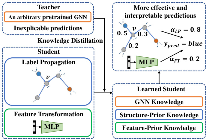
Figure 1: An overview of our knowledge distillation framework. The two simple prediction mechanisms of our student model ensure the full use of structure/feature-based prior knowledge. The knowledge in GNN teachers will be extracted and injected into the student during knowledge distillation. Thus the student can go beyond its corresponding teacher with more effective predictions.
图 1: 我们的知识蒸馏框架概览。学生模型的两个简单预测机制确保充分利用基于结构/特征的先验知识。GNN教师模型中的知识将在知识蒸馏过程中被提取并注入学生模型,使学生能够超越其对应的教师模型,实现更有效的预测。
April 19–23, 2021 ,Ljubljana, Slovenia. ACM, New York, NY, USA, 11 pages. https://doi.org/10.1145/3442381.3450068
2021年4月19日至23日,斯洛文尼亚卢布尔雅那。ACM,美国纽约州纽约市,11页。https://doi.org/10.1145/3442381.3450068
1 INTRODUCTION
1 引言
Semi-supervised learning on graph-structured data aims at classifying every node in a network given the network structure and a subset of nodes labeled. As a fundamental task in graph analysis [3], the classification problem has a wide range of real-world applications such as user profiling [15], recommend er systems [28], text classification [1] and sociological studies [2]. Most of these applications have the homophily phenomenon [16], which assumes two linked nodes tend to have similar labels. With the homophily assumption, many traditional methods are developed to propagate labels by random walks [27, 39] or regularize the label differences between neighbors [9, 36].
图结构数据上的半监督学习旨在给定网络结构和部分已标注节点的条件下,对网络中每个节点进行分类。作为图分析中的基础任务[3],该分类问题在用户画像[15]、推荐系统[28]、文本分类[1]和社会学研究[2]等现实场景中具有广泛应用。大多数应用场景存在同质性现象[16],即假设相连节点往往具有相似标签。基于同质性假设,传统方法主要通过随机游走[27,39]或邻居节点间标签差异正则化[9,36]来实现标签传播。
With the success of deep learning, methods based on graph neural networks (GNNs) [7, 11, 29] have demonstrated their effec ti ve ness in classifying node labels. Most GNN models adopt message passing strategy [6]: each node aggregates features from its neighborhood and then a layer-wise projection function with a non-linear activation will be applied to the aggregated information. In this way, GNNs can utilize both graph structure and node feature information in their models.
随着深度学习的成功,基于图神经网络 (graph neural networks, GNNs) [7, 11, 29] 的方法在节点标签分类任务中展现了其有效性。大多数GNN模型采用消息传递策略 [6]:每个节点聚合其邻域特征,然后对聚合信息应用带有非线性激活的逐层投影函数。通过这种方式,GNNs能够在模型中同时利用图结构和节点特征信息。
However, the entanglement of graph topology, node features and projection matrices in GNNs leads to a complicated prediction mechanism and could not take full advantage of prior knowledge lying in the data. For example, the aforementioned homophily assumption adopted in label propagation methods represents structure-based prior, and has been shown to be underused [14, 30] in graph convolutional network (GCN) [11].
然而,图神经网络(GNN)中图拓扑、节点特征和投影矩阵的纠缠导致了复杂的预测机制,无法充分利用数据中的先验知识。例如,标签传播方法采用的同质性假设代表了基于结构的先验,但研究表明图卷积网络(GCN) [11] 并未充分运用这一先验 [14, 30]。
As an evidence, recent studies proposed to incorporate the label propagation mechanism into GCN by adding regular iz at ions [30] or manipulating graph filters [14, 24]. Their experimental results show that GCN can be improved by emphasizing such structure-based prior knowledge. Nevertheless, these methods have three major drawbacks: (1) The main bodies of their models are still GNNs and thus hard to fully utilize the prior knowledge; (2) They are single models rather than frameworks, and thus not compatible with other advanced GNN architectures; (3) They ignored another important prior knowledge, i.e., feature-based prior, which means that a node’s label is purely determined by its own features.
作为佐证,近期研究提出通过添加正则化项 [30] 或操纵图滤波器 [14, 24] 将标签传播机制融入 GCN。实验结果表明,强调这类基于结构的先验知识可以改进 GCN。然而,这些方法存在三个主要缺陷:(1) 模型主体仍为 GNN,难以充分利用先验知识;(2) 属于单一模型而非框架,无法兼容其他先进 GNN 架构;(3) 忽略了另一重要先验知识——基于特征的先验,即节点标签完全由其自身特征决定。
To address these issues, we propose an effective knowledge distillation framework to inject the knowledge of an arbitrary learned GNN (teacher model) into a well-designed student model. The student model is built with two simple prediction mechanisms, i.e., label propagation and feature transformation, which naturally preserves structure-based and feature-based prior knowledge, respectively. In specific, we design the student model as a trainable combination of parameterized label propagation and feature-based 2-layer MLP (Multi-layer Perceptron). On the other hand, it has been recognized that the knowledge of a teacher model lies in its soft predictions [8]. By simulating the soft labels predicted by a teacher model, our student model is able to further make use of the knowledge in pretrained GNNs. Consequently, the learned student model has a more interpret able prediction process and can utilize both GNN and structure/feature-based priors. An overview of our framework is shown in Fig. 1.
为解决这些问题,我们提出了一种有效的知识蒸馏框架,将任意已训练GNN(教师模型)的知识注入精心设计的学生模型中。该学生模型采用两种简单预测机制构建:标签传播和特征变换,分别天然保留了基于结构和基于特征的先验知识。具体而言,我们将学生模型设计为参数化标签传播与基于特征的双层MLP(多层感知机)的可训练组合。另一方面,学界公认教师模型的知识蕴含在其软预测中[8]。通过模拟教师模型预测的软标签,我们的学生模型能够进一步利用预训练GNN中的知识。因此,学习得到的学生模型具备更可解释的预测过程,并能同时利用GNN与结构/特征先验。图1展示了我们框架的总体结构。
We conduct experiments on five public benchmark datasets and employ several popular GNN models including GCN [11], GAT [29], SAGE [7], APPNP [12], SGC [32] and a recent deep GCN model GCNII [4] as teacher models. Experimental results show that a student model is able to outperform its corresponding teacher model by $1.4%\sim4.7%$ in terms of classification accuracy. It is worth noting that we also apply our framework on GLP [14] which unified GCN and label propagation by manipulating graph filters. As a result, we can still gain $1.5%\sim2.3%$ relative improvements, which demonstrates the potential compatibility of our framework. Furthermore, we investigate the interpret ability of our student model by probing the learned balance parameters between parameterized label propagation and feature transformation as well as the learned confidence score of each node in label propagation. To conclude, the improvements are consistent and significant with better interpret ability.
我们在五个公开基准数据集上进行实验,并采用多种流行GNN模型作为教师模型,包括GCN [11]、GAT [29]、SAGE [7]、APPNP [12]、SGC [32]以及近期提出的深度GCN模型GCNII [4]。实验结果表明,学生模型在分类准确率上能超越对应教师模型$1.4%\sim4.7%$。值得注意的是,我们还将该框架应用于通过操纵图滤波器统一GCN与标签传播的GLP [14],仍能获得$1.5%\sim2.3%$的相对提升,这证明了我们框架的潜在兼容性。此外,我们通过探查参数化标签传播与特征变换之间的学习平衡参数,以及标签传播中每个节点的学习置信度分数,研究了学生模型的可解释性。总体而言,该改进具有一致性和显著性,同时具备更好的可解释性。
The contributions of this paper are summarized as follows:
本文的贡献总结如下:
• We propose an effective knowledge distillation framework to extract the knowledge of an arbitrary pretrained GNN model and inject it into a student model for more effective predictions.
• 我们提出了一种有效的知识蒸馏框架,用于提取任意预训练图神经网络 (GNN) 模型的知识,并将其注入学生模型以实现更有效的预测。
• We design the student model as a trainable combination of parameterized label propagation and feature-based 2-layer MLP.
• 我们将学生模型设计为可训练的参数化标签传播与基于特征的2层MLP组合。
Hence the student model has a more interpret able prediction process and naturally preserves the structure/feature-based priors. Consequently, the learned student model can utilize both GNN and prior knowledge.
因此,学生模型具有更可解释的预测过程,并自然地保留了基于结构/特征的先验知识。这使得学习到的学生模型能够同时利用图神经网络(GNN)和先验知识。
• Experimental results on five benchmark datasets with seven GNN teacher models demonstrate the effectiveness of our framework. Extensive studies by probing the learned weights in the student model also illustrate the potential interpret ability of our method.
• 在五个基准数据集上使用七种GNN教师模型的实验结果表明了我们框架的有效性。通过探究学生模型中学习到的权重进行的广泛研究,也展示了我们方法潜在的 interpret ability (可解释性)。
2 RELATED WORK
2 相关工作
This work is most relevant to graph neural network models and knowledge distillation methods.
本工作主要涉及图神经网络模型和知识蒸馏方法。
2.1 Graph Neural Networks
2.1 图神经网络 (Graph Neural Networks)
The concept of GNN was proposed [21] before 2010 and has become a rising topic since the emergence of GCN [11]. During the last five years, graph neural network models have achieved promising results in many research areas [33, 37]. Now we will briefly introduce some representative GNN methods in this section and employ them as our teacher models in the experiments.
GNN的概念在2010年之前就被提出[21],并随着GCN[11]的出现成为热门话题。过去五年中,图神经网络模型在许多研究领域取得了显著成果[33, 37]。本节将简要介绍几种代表性GNN方法,并将其作为实验中的教师模型。
As one of the most influential GNN models, Graph Convolutional Network (GCN) [11] targeted on semi-supervised learning on graph-structured data through layer-wise propagation of node features. GCN can be interpreted as a variant of convolutional neural networks that operates on graphs. Graph Attention Network (GAT) [29] further employed attention mechanism in the aggregation of neighbors’ features. SAGE [7] sampled and aggregated features from a node’s local neighborhood and is more spaceefficient. Approximate personalized propagation of neural predictions (APPNP) [12] studied the relationship between GCN and PageRank, and incorporated a propagation scheme derived from personalized PageRank into graph filters. Simple Graph Convolution (SGC) [32] simplified GCN by removing non-linear activations and collapsing weight matrices between layers. Graph Convolutional Network via Initial residual and Identity mapping (GCNII) [4] was a very recent deep GCN model which alleviates the over-smoothing problem.
作为最具影响力的图神经网络 (GNN) 模型之一,图卷积网络 (Graph Convolutional Network, GCN) [11] 通过节点特征的层级传播,专注于图结构数据的半监督学习。GCN 可视为在图数据上运行的卷积神经网络变体。图注意力网络 (Graph Attention Network, GAT) [29] 进一步在邻居特征聚合中引入注意力机制。SAGE [7] 通过采样和聚合节点局部邻域特征实现了更高空间效率。神经预测近似个性化传播 (Approximate personalized propagation of neural predictions, APPNP) [12] 研究了 GCN 与 PageRank 的关系,并将个性化 PageRank 派生的传播方案融入图滤波器。简单图卷积 (Simple Graph Convolution, SGC) [32] 通过移除非线性激活函数和压缩层间权重矩阵简化了 GCN。基于初始残差与恒等映射的图卷积网络 (Graph Convolutional Network via Initial residual and Identity mapping, GCNII) [4] 是最新提出的深度 GCN 模型,有效缓解了过平滑问题。
Recently, several works show that the performance of GNNs can be further improved by incorporating traditional prediction mechanisms, i.e., label propagation. For example, Generalized Label Propagation (GLP) [14] modified graph convolutional filters to generate smooth features with graph similarity encoded. UniMP [24] fused feature aggregation and label propagation by a shared messagepassing network. GCN-LPA [30] employed label propagation as regular iz ation to assist GCN for better performances. Note that the label propagation mechanism was built with simple structurebased prior knowledge. Their improvements indicate that such prior knowledge is not fully explored in GNNs. Nevertheless, these advanced models still suffer from several drawbacks as illustrated in the Introduction section.
最近,多项研究表明,通过结合传统预测机制(即标签传播)可以进一步提升图神经网络(GNN)的性能。例如,广义标签传播(GLP)[14]通过修改图卷积滤波器来生成具有图相似性编码的平滑特征;UniMP[24]通过共享的消息传递网络融合了特征聚合与标签传播;GCN-LPA[30]则利用标签传播作为正则化手段来辅助图卷积网络(GCN)获得更好表现。值得注意的是,标签传播机制是基于简单的结构先验知识构建的,这些改进表明此类先验知识在GNN中尚未得到充分探索。然而,如引言部分所述,这些先进模型仍存在若干缺陷。
2.2 Knowledge Distillation
2.2 知识蒸馏
Knowledge distillation [8] was proposed for model compression where a small light-weight student model is trained to mimic the soft predictions of a pretrained large teacher model. After the distillation, the knowledge in the teacher model will be transferred into the student model. In this way, the student model can reduce time and space complexities without losing prediction qualities. Knowledge distillation is widely used in the computer vision area, e.g., a deep convolutional neural network (CNN) will be compressed into a shallow one to accelerate the inference.
知识蒸馏 [8] 是一种模型压缩方法,通过训练轻量级的学生模型来模仿预训练大型教师模型的软预测结果。蒸馏完成后,教师模型中的知识将被迁移到学生模型中。这种方式使学生模型能在保持预测质量的同时降低时间和空间复杂度。知识蒸馏在计算机视觉领域应用广泛,例如将深度卷积神经网络 (CNN) 压缩为浅层网络以加速推理。
In fact, there are also a few studies combining knowledge distillation with GCN. However, their motivation and model architecture are quite different from ours. Yang et al. [34] which was proposed in the computer vision area, compressed a deep GCN with large feature maps into a shallow one with fewer parameters using a local structure preserving module. Reliable Data Distillation (RDD) [35] trained multiple GCN students with the same architecture and then ensembled them for better performance in a manner similar to BAN [5]. Graph Markov Neural Networks (GMNN) [19] can also be viewed as a knowledge distillation method where two GCNs with different reception sizes learn from each other. Note that both teacher and student models in these works are GCNs.
事实上,也有少数研究将知识蒸馏 (knowledge distillation) 与图卷积网络 (GCN) 相结合。但它们的研究动机和模型架构与我们的工作存在显著差异。Yang等人[34](源自计算机视觉领域)通过局部结构保留模块,将具有大型特征图的深层GCN压缩为参数更少的浅层网络。可靠数据蒸馏 (RDD) [35] 采用与BAN[5]类似的方式,训练多个相同架构的GCN学生模型并通过集成提升性能。图马尔可夫神经网络 (GMNN) [19] 也可视为一种知识蒸馏方法,其中两个具有不同感受野的GCN相互学习。值得注意的是,这些工作中的教师模型和学生模型均为GCN架构。
Compared with them, the goal of our framework is to extract the knowledge of GNNs and go beyond it. Our framework is very flexible and can be applied on an arbitrary GNN model besides GCN. We design a student model with simple prediction mechanisms and thus are able to benefit from both GNN and prior knowledge. As the output of our framework, the student model also has a more interpret able prediction process. In terms of training details, our framework is simpler and requires no ensembling or iterative distillations between teacher and student models for improving classification accuracies.
与它们相比,我们框架的目标是提取图神经网络 (GNN) 的知识并超越其局限。该框架具有高度灵活性,除图卷积网络 (GCN) 外可应用于任意 GNN 模型。我们设计了具有简单预测机制的学生模型,从而能同时受益于 GNN 和先验知识。作为框架的输出产物,该学生模型还具备更可解释的预测过程。在训练细节方面,我们的框架更简洁,无需通过师生模型集成或迭代蒸馏来提升分类准确率。
3 METHODOLOGY
3 方法论
In this section, we will start by formalizing the semi-supervised node classification problem and introducing the notations. Then we will present our knowledge distillation framework to extract the knowledge of GNNs. Afterwards, we will propose the architecture of our student model, which is a trainable combination of parameterized label propagation and feature-based 2-layer MLP. Finally, we will discuss the potential interpret ability of the student model and the computation complexity of our framework.
在本节中,我们将首先形式化半监督节点分类问题并介绍相关符号。随后提出用于提取图神经网络 (GNN) 知识的知识蒸馏框架。接着介绍学生模型的架构——该模型由参数化标签传播和基于特征的双层多层感知机 (MLP) 可训练组合构成。最后将探讨学生模型的潜在可解释性及本框架的计算复杂度。
3.1 Semi-supervised Node Classification
3.1 半监督节点分类
We begin by outlining the problem of node classification. Given a connected graph $G=(V,E)$ with a subset of nodes $V_{L}\subset V$ labeled, where $V$ is the vertex set and $E$ is the edge set, node classification targets on predicting the node labels for every node $v$ in unlabeled node set $V_{U}=V\setminus V_{L}$ . Each node $v\in V$ has label $y_{v}\in Y$ where $Y$ is the set of all possible labels. In addition, node features $X\in\mathbb{R}^{|V|\times d}$ are usually available in graph data and can be utilized for better classification accuracy. Each row $X_{v}\in\mathbb{R}^{d}$ of matrix $X$ denotes a $d$ -dimensional feature vector of node $v$ .
我们首先概述节点分类问题。给定一个连通图 $G=(V,E)$,其中部分节点 $V_{L}\subset V$ 带有标签($V$ 为顶点集,$E$ 为边集),节点分类的目标是预测未标记节点集 $V_{U}=V\setminus V_{L}$ 中每个节点 $v$ 的标签。每个节点 $v\in V$ 的标签为 $y_{v}\in Y$,其中 $Y$ 是所有可能标签的集合。此外,图数据通常包含节点特征 $X\in\mathbb{R}^{|V|\times d}$,可用于提升分类准确率。矩阵 $X$ 的每一行 $X_{v}\in\mathbb{R}^{d}$ 表示节点 $v$ 的 $d$ 维特征向量。
3.2 The Knowledge Distillation Framework
3.2 知识蒸馏框架
Node classification approaches including GNNs can be summarized as a black box that outputs a classifier $f$ given graph structure $G$ labeled node set $V_{L}$ and node feature $X$ as inputs. The classifier $f$ will predict the probability $f(v,y)$ that unlabeled node $v\in V_{U}$ has label $y\in Y$ , where $\begin{array}{r}{\sum_{y^{\prime}\in Y}f(v,y^{\prime})=1}\end{array}$ . For labeled node $v$ , we set $f(v,y)=1$ if $v$ is annotated with label $y$ and $f(v,y^{\prime})=0$ for any other label $y^{\prime}$ . We use $f(v)\in\mathbb{R}^{|Y|}$ to denote the probability distribution over all labels for brevity.
包括图神经网络 (GNN) 在内的节点分类方法可以概括为一个黑盒,该黑盒以图结构 $G$、带标签的节点集 $V_{L}$ 和节点特征 $X$ 作为输入,输出分类器 $f$。分类器 $f$ 将预测未标记节点 $v\in V_{U}$ 具有标签 $y\in Y$ 的概率 $f(v,y)$,其中 $\begin{array}{r}{\sum_{y^{\prime}\in Y}f(v,y^{\prime})=1}\end{array}$。对于带标签的节点 $v$,如果 $v$ 被标注为标签 $y$,则设 $f(v,y)=1$,对于任何其他标签 $y^{\prime}$,设 $f(v,y^{\prime})=0$。为简洁起见,我们使用 $f(v)\in\mathbb{R}^{|Y|}$ 表示所有标签上的概率分布。
In this paper, the teacher model employed in our framework can be an arbitrary GNN model such as GCN [11] or GAT [29]. We denote the pretrained classifier in a teacher model as $f_{G N N}$ On the other hand, we use 𝑓𝑆𝑇𝑈 ;Θ to denote the student model parameterized by $\Theta$ and $f_{S T U;\Theta}(v)\in\mathbb{R}^{|Y|}$ represents the predicted probability distribution of node $v$ by the student.
本文框架中采用的教师模型可以是任意图神经网络模型,例如 GCN [11] 或 GAT [29]。我们将教师模型中的预训练分类器表示为 $f_{G N N}$,同时使用参数化学生模型的 $f_{S T U;\Theta}$ 表示由 $\Theta$ 参数化的学生模型,其中 $f_{S T U;\Theta}(v)\in\mathbb{R}^{|Y|}$ 表示学生模型对节点 $v$ 的预测概率分布。
In knowledge distillation [8], the student model is trained to mimic the soft label predictions of a pretrained teacher model. As a result, the knowledge lying in the teacher model will be extracted and injected into the learned student. Therefore, the optimization objective which aligns the outputs between the student model and pretrained teacher model can be formulated as
在知识蒸馏 [8] 中,学生模型通过模仿预训练教师模型的软标签预测进行训练。这样,教师模型中的知识将被提取并注入到学习中的学生模型中。因此,对齐学生模型与预训练教师模型输出的优化目标可以表述为

where 𝑑𝑖𝑠𝑡𝑎𝑛𝑐𝑒 $(\cdot,\cdot)$ measures the distance between two predicted probability distributions. Specifically, we use Euclidean distance in this work1.
其中 $distance$ $(\cdot,\cdot)$ 用于衡量两个预测概率分布之间的距离。具体而言,本研究采用欧氏距离1。
3.3 The Architecture of Student Model
3.3 学生模型架构
We hypothesize that a node’s label prediction follows two simple mechanisms: (1) label propagation from its neighboring nodes and (2) a transformation from its own features. Therefore, as shown in Fig. 2, we design our student model as a combination of these two mechanisms, i.e., a Parameterized Label Propagation (PLP) module and a Feature Transformation (FT) module, which can naturally preserve the structure/feature-based prior knowledge, respectively. After the distillation, the student will benefit from both GNN and prior knowledge with a more interpret able prediction mechanism.
我们假设节点的标签预测遵循两种简单机制:(1) 来自相邻节点的标签传播 (2) 自身特征转换。因此如图 2 所示,我们将学生模型设计为这两种机制的组合,即参数化标签传播 (PLP) 模块和特征转换 (FT) 模块,它们能分别自然地保留基于结构/特征的先验知识。蒸馏后,学生模型将通过更可解释的预测机制,同时受益于图神经网络和先验知识。
In this subsection, we will first briefly review the conventional label propagation algorithm. Then we will introduce our PLP and FT modules as well as their trainable combinations.
在本小节中,我们将首先简要回顾传统的标签传播算法,随后介绍我们的PLP和FT模块及其可训练组合方案。
3.3.1 Label Propagation. Label propagation (LP) [38] is a classical graph-based semi-supervised learning model. This model simply follows the assumption that nodes linked by an edge (or occupying the same manifold) are very likely to share the same label. Based on this hypothesis, labels will propagate from labeled nodes to unlabeled ones for predictions.
3.3.1 标签传播。标签传播 (LP) [38] 是一种经典的基于图的半监督学习模型。该模型遵循一个简单假设:通过边连接的节点(或位于同一流形上的节点)很可能共享相同标签。基于这一假设,标签将从已标注节点传播至未标注节点以进行预测。
Formally, we use $f_{L P}$ to denote the final prediction of LP and $f_{L P}^{k}$ to denote the prediction of LP after $k$ iterations. In this work, we initialize the prediction of node 𝑣 as a one-hot label vector if $v$ is a labeled node. Otherwise, we will set a uniform label distribution for each unlabeled node $v$ , which indicates that the probabilities of all classes are the same at the beginning. The initialization can be formalized as:
形式上,我们用 $f_{L P}$ 表示 LP (Label Propagation) 的最终预测结果,用 $f_{L P}^{k}$ 表示经过 $k$ 次迭代后的 LP 预测结果。在本工作中,如果节点 𝑣 是已标注节点,我们将其预测初始化为一个独热 (one-hot) 标签向量;否则,我们会为每个未标注节点 𝑣 设置一个均匀的标签分布,表示初始时所有类别的概率相同。该初始化过程可形式化表示为:
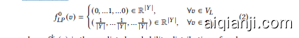
where $f_{L P}^{k}(v)$ is the predicted probability distribution of node $v$ at iteration $k$ . In the $k+1$ -th iteration, LP will update the label
其中 $f_{L P}^{k}(v)$ 是节点 $v$ 在第 $k$ 次迭代时的预测概率分布。在第 $k+1$ 次迭代中,LP将更新标签
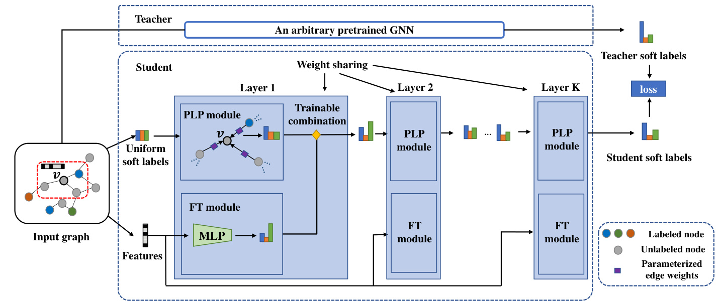
Figure 2: An illustration of the architecture of our proposed student model. Taking the center node 𝑣 as an example, the student model starts from node 𝑣’s raw features and a uniform label distribution as soft labels. Then at each layer, the soft label prediction of 𝑣 will be updated as a trainable combination of Parameterized Label Propagation (PLP) from 𝑣’s neighbors and Feature Transformation (FT) of 𝑣’s features. Finally, the distance between the soft label predictions of student and pretrained teacher will be minimized.
图 2: 我们提出的学生模型架构示意图。以中心节点 𝑣 为例,学生模型从节点 𝑣 的原始特征和均匀标签分布作为软标签开始。然后在每一层,𝑣 的软标签预测将通过可训练的参数化标签传播 (PLP) 和特征变换 (FT) 的组合进行更新。最终,学生模型与预训练教师模型的软标签预测之间的距离将被最小化。
predictions of each unlabeled node $v\in V_{U}$ as follows:
对每个未标记节点 $v\in V_{U}$ 的预测如下:
$$
f_{L P}^{k+1}(v)=(1-\lambda)\frac{1}{\vert N_{v}\vert}\sum_{u\in N_{v}}{f_{L P}^{k}(u)}+\lambda f_{L P}^{k}(v),
$$
$$
f_{L P}^{k+1}(v)=(1-\lambda)\frac{1}{\vert N_{v}\vert}\sum_{u\in N_{v}}{f_{L P}^{k}(u)}+\lambda f_{L P}^{k}(v),
$$
where $N_{v}$ is the set of node $v$ ’s neighbors in the graph and $\lambda$ is a hyper-parameter controlling the smoothness of node updates.
其中 $N_{v}$ 是图中节点 $v$ 的邻居集合,$\lambda$ 是控制节点更新平滑度的超参数。
Note that LP has no parameters to be trained, and thus can not fit the output of a teacher model through end-to-end training. Therefore, we retrofit LP by introducing more parameters to increase its capacity.
需要注意的是,LP (Label Propagation) 没有需要训练的参数,因此无法通过端到端训练来拟合教师模型的输出。为此,我们通过引入更多参数来改进 LP,以提升其能力。
3.3.2 Parameterized Label Propagation Module. Now we will introduce our Parameterized Label Propagation (PLP) module by further parameter i zing edge weights in LP. As shown in Eq. 3, LP model treats all neighbors of a node equally during the propagation. However, we hypothesize that the importance of different neighbors to a node should be different, which determines the propagation intensities between nodes. To be more specific, we assume that the label predictions of some nodes are more “confident” than others: e.g., a node whose predicted label is similar to most of its neighbors. Such nodes will be more likely to propagate their labels to neighbors and keep themselves unchanged.
3.3.2 参数化标签传播模块
现在我们通过进一步参数化LP中的边权重来介绍参数化标签传播(PLP)模块。如公式3所示,LP模型在传播过程中平等对待节点的所有邻居。但我们假设不同邻居对节点的重要性应当不同,这决定了节点间的传播强度。具体而言,我们认为某些节点的标签预测比其他节点更"可信":例如预测标签与其多数邻居相似的节点。这类节点更可能将标签传播给邻居并保持自身不变。
Formally, we will assign a confidence score $c_{v}\in\mathbb{R}$ to each node 𝑣. During the propagation, all node 𝑣’s neighbors and $v$ itself will compete to propagate their labels to 𝑣. Following the intuition that a larger confidence score will have a larger edge weight, we rewrite the prediction update function in Eq. 3 for $f_{P L P}$ as follows:
形式上,我们将为每个节点𝑣分配一个置信度分数$c_{v}\in\mathbb{R}$。在传播过程中,节点𝑣的所有邻居及其自身将竞争向𝑣传播它们的标签。基于置信度分数越大则边权重越大的直觉,我们将式(3)中的预测更新函数$f_{PLP}$重写如下:
$$
f_{P L P}^{k+1}(v)=\sum_{u\in N_{v}\cup{v}}w_{u v}f_{P L P}^{k}(u),
$$
$$
f_{P L P}^{k+1}(v)=\sum_{u\in N_{v}\cup{v}}w_{u v}f_{P L P}^{k}(u),
$$
where $w_{u v}$ is the edge weight between node $u$ and $v$ computed by the following softmax function:
其中 $w_{u v}$ 是节点 $u$ 和 $v$ 之间的边权重,由以下 softmax 函数计算得出:
$$
w_{u v}=\frac{e x p(c_{u})}{\sum_{u^{\prime}\in N_{v}\cup{v}}e x p(c_{u^{\prime}})}.
$$
$$
w_{u v}=\frac{e x p(c_{u})}{\sum_{u^{\prime}\in N_{v}\cup{v}}e x p(c_{u^{\prime}})}.
$$
Similar to LP, $f_{P L P}^{0}(v)$ is initialized as Eq. 2 and $f_{P L P}^{k}(v)$ remains the one-hot ground truth label vector for every labeled node $v\in V_{L}$ during the propagation.
与 LP 类似,$f_{P L P}^{0}(v)$ 初始化为公式 2,且在传播过程中每个已标注节点 $v\in V_{L}$ 的 $f_{P L P}^{k}(v)$ 始终保持独热编码的真实标签向量。
Note that we can further parameter ize confidence score $c_{v}$ for inductive setting as an optional choice:
注意,我们可以进一步将置信度分数 $c_{v}$ 参数化为归纳设置的可选方案:
$$
\begin{array}{r}{c_{v}=z^{T}X_{v},}\end{array}
$$
$$
\begin{array}{r}{c_{v}=z^{T}X_{v},}\end{array}
$$
where $z\in\mathbb{R}^{d}$ is a learnable parameter that projects node $v$ ’s feature into the confidence score.
其中 $z\in\mathbb{R}^{d}$ 是一个可学习参数,用于将节点 $v$ 的特征投影为置信度分数。
3.3.3 Feature Transformation Module. Note that PLP module which propagates labels through edges emphasizes the structure-based prior knowledge. Thus we also introduce Feature Transformation (FT) module as a complementary prediction mechanism. The FT module predicts labels by only looking at the raw features of a node. Formally, denoting the prediction of FT module as $f_{F T}$ , we apply a 2-layer $\mathrm{MLP^{2}}$ followed by a softmax function to transform the features into soft label predictions:
3.3.3 特征转换模块。需要注意的是,通过边传播标签的PLP模块强调基于结构的先验知识。因此,我们引入特征转换(FT)模块作为补充预测机制。该模块仅通过观察节点的原始特征进行标签预测。形式上,将FT模块的预测表示为$f_{F T}$,我们采用2层$\mathrm{MLP^{2}}$后接softmax函数,将特征转换为软标签预测:
$$
f_{F T}(v)=s o f t m a x(M L P(X_{v})).
$$
$$
f_{F T}(v)=s o f t m a x(M L P(X_{v})).
$$
3.3.4 A Trainable Combination. Now we will combine the PLP and FT modules as the full model of our student. In detail, we will learn a trainable parameter $\alpha_{v}\in[0,1]$ for each node $v$ to balance the predictions between PLP and FT. In other words, the prediction from FT module will be incorporated into that from PLP at each propagation step. We name the full student model as Combination of Parameterized label propagation and Feature transformation (CPF) and thus the prediction update function for each unlabeled node $v\in V_{U}$ in Eq. 4 will be rewritten as
3.3.4 可训练组合。现在我们将PLP和FT模块组合为完整的学生模型。具体而言,我们会为每个节点$v$学习一个可训练参数$\alpha_{v}\in[0,1]$,以平衡PLP和FT之间的预测。换句话说,FT模块的预测将在每个传播步骤中融入PLP的预测。我们将完整的学生模型命名为参数化标签传播与特征变换的组合(CPF),因此式4中每个未标记节点$v\in V_{U}$的预测更新函数将被重写为
$$
f_{C P F}^{k+1}(v)=\alpha_{v}\sum_{u\in N_{v}\cup{v}}w_{u v}f_{C P F}^{k}(u)+(1-\alpha_{v})f_{F T}(v),
$$
$$
f_{C P F}^{k+1}(v)=\alpha_{v}\sum_{u\in N_{v}\cup{v}}w_{u v}f_{C P F}^{k}(u)+(1-\alpha_{v})f_{F T}(v),
$$
where edge weight $w_{u v}$ and initialization $f_{C P F}^{0}(v)$ are the same with PLP module. Whether parameter i zing confidence score $c_{v}$ as Eq. 6 or not will lead to inductive/trans duct ive variants CPF-ind/CPF-tra.
其中边权重 $w_{u v}$ 和初始化 $f_{C P F}^{0}(v)$ 与PLP模块相同。是否如式6所示参数化置信分数 $c_{v}$ 将分别得到归纳型/传导型变体CPF-ind/CPF-tra。
3.4 The Overall Algorithm and Details
3.4 整体算法与细节
Assuming that our student model has a total of $K$ layers, the distillation objective in Eq. 1 can be detailed as:
假设我们的学生模型共有 $K$ 层,则公式 1 中的蒸馏目标可细化为:

where $|cdot|{2}$ is the L2-norm and the parameter set $Theta$ includes the balancing parameters between PLP and FT ${\alpha{v},\forall v\in V}$ , confidence parameters in PLP module ${c{v},\forall v\in V}$ (or parameter $z$ for induc- tive setting), and the parameters of MLP in FT module $\Theta_{M L P}$ . There is also an important hyper-parameter in the distillation framework: the number of propagation layers $K$ . Alg. 1 shows the pseudo code of the training process.
其中 $|cdot|{2}$ 表示 L2 范数,参数集 $ Theta$ 包含 PLP 与 FT 之间的平衡参数 ${\alpha{v},\forall v\in V}$、PLP 模块中的置信度参数 ${c{v},\forall v\in V}$ (或归纳设置中的参数 $z$),以及 FT 模块中 MLP 的参数 $\Theta{M L P}$。蒸馏框架中还有一个重要超参数:传播层数 $K$。算法 1 展示了训练过程的伪代码。
We implement our framework based on Deep Graph Library (DGL) [31] and Pytorch [18], and employ an Adam optimizer [10] for parameter training. Dropout [25] is also applied to alleviate over fitting.
我们基于深度图库 (DGL) [31] 和 Pytorch [18] 实现了框架,并采用 Adam 优化器 [10] 进行参数训练。同时应用了 Dropout [25] 来缓解过拟合问题。
Algorithm 1 The proposed knowledge distillation framework.
算法 1: 提出的知识蒸馏框架
3.5 Discussions on Interpret ability and Complexity
3.5 可解释性与复杂性的讨论
In this subsection, we will discuss the interpret ability of the learned student model and the complexity of our algorithm.
在本小节中,我们将讨论所学学生模型的可解释性以及我们算法的复杂性。
After the knowledge distillation, our student model CPF will predict the label of a specific node $v$ as a weighted average between the predictions of label propagation and feature-based MLP. The balance parameter $\alpha_{v}$ indicates whether structure-based LP or feature-based MLP is more important for node 𝑣’s prediction. LP mechanism is almost transparent and we can easily find out node $v$ is influenced by which neighbor to what extent at each iteration. On the other hand, the understanding of feature-based MLP can be derived by existing works [20] or directly looking at the gradients of different features. Therefore, the learned student model has better interpret ability than GNN teachers.
经过知识蒸馏后,我们的学生模型CPF会将特定节点$v$的标签预测为标签传播和基于特征的MLP预测结果之间的加权平均值。平衡参数$\alpha_{v}$表明对于节点𝑣的预测,基于结构的LP还是基于特征的MLP更为重要。LP机制几乎是透明的,我们可以轻松地发现节点$v$在每次迭代中受到哪些邻居的影响以及影响程度。另一方面,基于特征的MLP的理解可以通过现有研究[20]或直接查看不同特征的梯度来获得。因此,学习到的学生模型比GNN教师模型具有更好的可解释性。
The time complexity of each iteration (line 3 to 13 in Alg. 1) and the space complexity of our algorithm are both $O(|E|+d|V|)$ , which is linear to the scale of datasets. In fact, the operations can be easily implemented in matrix form and the training process can be finished in seconds on real-world benchmark datasets with a single GPU device. Therefore, our proposed knowledge distillation framework is very time/space-efficient.
每次迭代的时间复杂度(算法1中第3至13行)和算法的空间复杂度均为 $O(|E|+d|V|)$ ,与数据集规模呈线性关系。实际上,这些操作可以轻松以矩阵形式实现,在单GPU设备上仅需数秒即可完成现实基准数据集的训练过程。因此,我们提出的知识蒸馏框架具有极高的时间/空间效率。
4 EXPERIMENTS
4 实验
In this section, we will start by introducing the datasets and teacher models used in our experiments. Then we will detail the experimental settings of teacher models and student variants. Afterwards, we will present quantitative results on evaluating semi-supervised node classification. We also conduct experiments under different numbers of propagation layers and training ratios to illustrate the robustness of our algorithm. Finally, we will present qualitative case studies and visualization s for better understandings of the learned parameters in our student model CPF.
在本节中,我们将首先介绍实验所用的数据集和教师模型,随后详细说明教师模型与学生变体的实验设置。接着展示半监督节点分类任务的量化评估结果,并通过不同传播层数和训练比例的实验验证算法鲁棒性。最后通过定性案例分析和可视化呈现,深入解析学生模型CPF的参数学习机制。
4.1 Datasets
4.1 数据集
Table 1: Dataset statistics.
表 1: 数据集统计。
| 数据集 | 节点数 | 边数 | 特征数 | 类别数 |
|---|---|---|---|---|
| Cora | 2,485 | 5,069 | 1,433 | 7 |
| Citeseer | 2,110 | 3,668 | 3,703 | 6 |
| Pubmed | 19,717 | 44,324 | 500 | 3 |
| A-Computers | 13,381 | 245,778 | 767 | 10 |
| A-Photo | 7,487 | 119,043 | 745 | 8 |
We use five public benchmark datasets for experiments and the statistics of the datasets are shown in Table 1. As previous works [13, 23, 26] did, we only consider the largest connected component and regard the edges as undirected. The details about the datasets are as follows:
我们使用五个公开基准数据集进行实验,数据集统计信息如表 1 所示。与先前工作 [13, 23, 26] 一致,我们仅考虑最大连通分量并将边视为无向边。各数据集详细信息如下:
• Cora [22] is a benchmark citation dataset composed of machine learning papers, where each node represents a document with a sparse bag-of-words feature vector. Edges represent citations between documents, and labels specify the research field of each paper.
• Cora [22] 是一个由机器学习论文组成的基准引用数据集,其中每个节点代表一个带有稀疏词袋 (bag-of-words) 特征向量的文档。边表示文档之间的引用关系,标签则标明每篇论文的研究领域。
Table 2: Classification accuracies with teacher models as GCN [11] and GAT [29].
表 2: 以 GCN [11] 和 GAT [29] 作为教师模型的分类准确率。
| Datasets | Teacher Studentvariants | +Impv. | Teacher | Studentvariants | +Impv. | |||||||
|---|---|---|---|---|---|---|---|---|---|---|---|---|
| GCN | PLP | FT | CPF-ind | CPF-tra | GAT | PLP | FT | CPF-ind | CPF-tra | |||
| Cora | 0.8244 | 0.7522 | 0.8253 | 0.8576 | 0.8567 | 4.0% | 0.8389 | 0.7578 | 0.8426 | 0.8576 | 0.8590 | 2.4% |
| Citeseer | 0.7110 | 0.6602 | 0.7055 | 0.7619 | 0.7652 | 7.6% | 0.7276 | 0.6624 | 0.7591 | 0.7657 | 0.7691 | 5.7% |
| Pubmed | 0.7804 | 0.6471 | 0.7964 | 0.8080 | 0.8104 | 3.8% | 0.7702 | 0.6848 | 0.7896 | 0.8011 | 0.8040 | 4.4% |
| A-Computers | 0.8318 | 0.7584 | 0.8356 | 0.8443 | 0.8443 | 1.5% | 0.8107 | 0.7605 | 0.8135 | 0.8190 | 0.8148 | 1.0% |
| A-Photo | 0.9072 | 0.8499 | 0.9265 | 0.9317 | 0.9248 | 2.7% | 0.8987 | 0.8496 | 0.9190 | 0.9221 | 0.9199 | 2.6% |
Table 3: Classification accuracies with teacher models as APPNP [12] and SAGE [7].
表 3: 以 APPNP [12] 和 SAGE [7] 作为教师模型的分类准确率。
| 数据集 | APPNP | PLP | FT | CPF-ind | CPF-tra | +Impv. | SAGE | PLP | FT | CPF-ind | CPF-tra | +Impv. |
|---|---|---|---|---|---|---|---|---|---|---|---|---|
| Cora | 0.8398 | 0.7251 | 0.8379 | 0.8581 | 0.8562 | 2.2% | 0.8178 | 0.7663 | 0.8201 | 0.8473 | 0.8454 | 3.6% |
| Citeseer | 0.7547 | 0.6812 | 0.7580 | 0.7646 | 0.7635 | 1.3% | 0.7171 | 0.6641 | 0.7425 | 0.7497 | 0.7575 | 5.6% |
| Pubmed | 0.7950 | 0.6866 | 0.8102 | 0.8058 | 0.8081 | 1.6% | 0.7736 | 0.6829 | 0.7717 | 0.7948 | 0.8062 | 4.2% |
| A-Computers | 0.8236 | 0.7516 | 0.8176 | 0.8279 | 0.8211 | 0.5% | 0.7760 | 0.7590 | 0.7912 | 0.7971 | 0.8199 | 5.7% |
| A-Photo | 0.9148 | 0.8469 | 0.9241 | 0.9273 | 0.9272 | 1.4% | 0.8863 | 0.8366 | 0.9153 | 0.9268 | 0.9248 | 4.6% |
• Citeseer [22] is another benchmark citation dataset of computer science publications, holding similar configuration to Cora. Citeseer dataset has the largest number of features among all five datasets used in this paper. • Pubmed [17] is also a citation dataset, consisting of articles related to diabetes in the PubMed database. The node features are TF/IDF weighted word frequency, and the label indicates the type of diabetes discussed in this article. • A-Computers and A-Photo [23] are extracted from Amazon co-purchase graph, where nodes represent products, edges represent whether two products are frequently co-purchased or not, features represent product reviews encoded by bagof-words, and labels are predefined product categories.
• Citeseer [22] 是另一个计算机科学文献的基准引用数据集,其配置与 Cora 类似。在本文使用的五个数据集中,Citeseer 数据集的特征数量最多。
• Pubmed [17] 同样是一个引用数据集,包含 PubMed 数据库中与糖尿病相关的文章。节点特征是经过 TF/IDF 加权的词频,标签表示文章中讨论的糖尿病类型。
• A-Computers 和 A-Photo [23] 是从亚马逊共同购买图中提取的数据集,其中节点代表商品,边表示两种商品是否经常被一起购买,特征是词袋模型编码的商品评论,标签是预定义的商品类别。
Following the experimental settings in previous work [23], we randomly sample 20 nodes from each class as labeled nodes, 30 nodes for validation and all other nodes for test.
根据先前工作[23]的实验设置,我们从每个类别中随机抽取20个节点作为标记节点,30个节点用于验证,其余所有节点用于测试。
4.2 Teacher Models and Settings
4.2 教师模型与设置
For a thorough comparison, we consider seven GNN models as teacher models in our knowledge distillation framework:
为了全面比较,我们在知识蒸馏框架中考虑了七种GNN模型作为教师模型:
The detailed training settings of teacher models are listed in Appendix A.
教师模型的详细训练设置见附录A。
4.3 Student Variants and Experimental Settings
4.3 学生变体与实验设置
For each dataset and teacher model, we test the following student variants:
对于每个数据集和教师模型,我们测试以下学生变体:
We randomly initialize the parameters and employ early stopping with a patience of 50, i.e., we will stop training if the classification accuracy on validation set does not increase for 50 epochs. For hyperparameter tuning, we conduct heuristic search by exploring layers $K\in{5,6,7,8,9,10}$ , hidden size in MLP $d_{M L P}\in{8,16,32,64}$ , dropout rate $d r\in{0.2,0.5,0.8}$ , learning rate and weight decay of Adam optimizer $l r\in{0.001,0.005,0.01}$ , $w d\in{0.0005,0.001,0.01}$ .
我们随机初始化参数,并采用早停策略 (patience=50),即若验证集分类准确率连续50轮未提升则停止训练。在超参数调优阶段,我们通过启发式搜索探索以下参数空间:层数 $K\in{5,6,7,8,9,10}$、MLP隐藏层维度 $d_{M L P}\in{8,16,32,64}$、丢弃率 $d r\in{0.2,0.5,0.8}$、Adam优化器的学习率 $l r\in{0.001,0.005,0.01}$ 和权重衰减系数 $w d\in{0.0005,0.001,0.01}$。
Table 4: Classification accuracies with teacher models as SGC [32] and GCNII [4].
表 4: 以 SGC [32] 和 GCNII [4] 作为教师模型的分类准确率。
| 数据集 | 教师学生变体 | +改进 | 教师 | 学生变体 | +改进 | |||||||
|---|---|---|---|---|---|---|---|---|---|---|---|---|
| SGC | PLP | FT | CPF-ind | CPF-tra | GCNII | PLP FT | CPF-ind | CPF-tra | ||||
| Cora | 0.8052 | 0.7513 | 0.8173 | 0.8454 | 0.8487 | 5.4% | 0.8384 | 0.7382 | 0.8431 | 0.8581 | 0.8590 | 2.5% |
| Citeseer | 0.7133 | 0.6735 | 0.7331 | 0.7470 | 0.7530 | 5.6% | 0.7376 | 0.6724 | 0.7564 | 0.7635 | 0.7569 | 3.5% |
| Pubmed | 0.7892 | 0.6018 | 0.8098 | 0.7972 | 0.8204 | 4.0% | 0.7971 | 0.6913 | 0.7984 | 0.7928 | 0.8024 | 0.7% |
| A-Computers | 0.8248 | 0.7579 | 0.8391 | 0.8367 | 0.8407 | 1.9% | 0.8325 | 0.7628 | 0.8411 | 0.8467 | 0.8447 | 1.7% |
| A-Photo | 0.9063 | 0.8318 | 0.9303 | 0.9397 | 0.9347 | 3.7% | 0.9230 | 0.8401 | 0.9263 | 0.9352 | 0.9300 | 1.3% |
Table 5: Classification accuracies with teacher model as GLP [14].
表 5: 以 GLP [14] 作为教师模型的分类准确率。
| 数据集 | 教师模型 | 学生模型变体 | 提升幅度 | |||
|---|---|---|---|---|---|---|
| GLP | PLP | FT | CPF-ind | CPF-tra | +Impv. | |
| Cora | 0.8365 | 0.7616 | 0.8314 | 0.8557 | 0.8539 | 2.3% |
| Citeseer | 0.7536 | 0.6630 | 0.7597 | 0.7696 | 0.7696 | 2.1% |
| Pubmed | 0.8088 | 0.6215 | 0.7842 | 0.8133 | 0.8210 | 1.5% |
4.4 Analysis of Classification Results
4.4 分类结果分析
Experimental results on five datasets with seven GNN teachers and four student variants are presented in Table 2, 3, 4 and $5^{3}$ . We have the following observations:
在五个数据集上使用七种GNN教师模型和四种学生变体的实验结果展示在表2、表3、表4和$5^{3}$中。我们得出以下观察结论:
• The proposed knowledge distillation framework accompanying with the full architecture of student model CPF-ind and CPF-tra, is able to improve the performance of the corresponding teacher model consistently and significantly. For example, the classification accuracy of GCN on Cora dataset is improved from 0.8244 to 0.8576. This is because the knowledge of GNN teachers can be extracted and injected into our student model which also benefits from structure/featurebased prior knowledge introduced by its simple prediction mechanism. This observation demonstrates our motivation and the effectiveness of our framework. • Note that the teacher model Generalized Label Propagation (GLP) [14] has already incorporated the label propagation mechanism in their graph filters. As shown in Table 5, we can still gain $1.5%\sim2.3%$ relative improvements by applying our knowledge distillation framework, which demonstrates the potential compatibility of our algorithm. • Among the four student variants, the full model CPF-ind and CPF-tra always perform best (except APPNP teacher on Pubmed dataset) and give competitive results. Thus both structure-based PLP and feature-based FT modules will contribute to the overall improvements. PLP itself performs worst because PLP which has few parameters to learn has a small model capacity and can not fit the soft predictions of teacher models. • The average relative improvements of the seven teachers GCN/GAT/APPNP/SAGE/SGC/GCNII/GLP are $3.9/3.2/1.4/$ $4.7/4.1/1.9/2.0%$ , respectively. The improvement over APPNP is the smallest. A possible reason is that APPNP preserves a
• 提出的知识蒸馏框架与学生模型CPF-ind和CPF-tra的完整架构相结合,能够持续显著提升对应教师模型的性能。例如,GCN在Cora数据集上的分类准确率从0.8244提升至0.8576。这是因为GNN教师模型的知识可以被提取并注入到学生模型中,同时该学生模型还受益于其简单预测机制引入的结构/特征先验知识。这一观察验证了我们的动机和框架的有效性。
• 值得注意的是,教师模型广义标签传播(GLP) [14] 已在图滤波器中融入了标签传播机制。如表5所示,通过应用我们的知识蒸馏框架仍能获得 $1.5%\sim2.3%$ 的相对提升,这证明了我们算法的潜在兼容性。
• 在四个学生模型变体中,完整模型CPF-ind和CPF-tra始终表现最佳(除Pubmed数据集上的APPNP教师模型外),并给出具有竞争力的结果。因此基于结构的PLP模块和基于特征的FT模块都对整体改进有所贡献。PLP本身表现最差,因为其可学习参数较少,模型容量小,无法拟合教师模型的软预测结果。
• 七种教师模型GCN/GAT/APPNP/SAGE/SGC/GCNII/GLP的平均相对改进分别为 $3.9/3.2/1.4/$ $4.7/4.1/1.9/2.0%$。对APPNP的改进最小,可能原因是APPNP保留了
node’s own features during the message passing and thus also utilizes the feature-based prior as our FT module does. • The average relative improvements on the five datasets Cora/ Citeseer/Pubmed/A-Computers/A-Photo are $2.9/4.2/2.7/2.1/$ $2.7%$ , respectively. Citeseer dataset benefits most from our knowledge distillation framework. A possible reason is that Citeseer has the largest number of features and thus the student model also has more trainable parameters to increase its capacity.
节点在消息传递过程中自身特征的同时,也像我们的FT模块那样利用了基于特征的先验知识。
• 在Cora/Citeseer/Pubmed/A-Computers/A-Photo五个数据集上的平均相对改进分别为$2.9/4.2/2.7/2.1/$ $2.7%$。其中Citeseer数据集从我们的知识蒸馏框架中受益最大,可能原因是该数据集特征数量最多,因此学生模型也拥有更多可训练参数来提升其能力。
4.5 Analysis of Different Numbers of Propagation Layers
4.5 不同传播层数的分析
In this subsection, we will investigate the influence of a key hyperparameter in the architecture of our student model CPF, i.e., the number of propagation layers $K$ . In fact, popular GNN models such as GCN and GAT are very sensitive to the number of layers. A larger number of layers will cause the over-smoothing issue and significantly harm the model performance. Hence we conduct experiments on Cora dataset for further analysis of this hyperparameter.
在本小节中,我们将研究学生模型CPF架构中的一个关键超参数——传播层数$K$的影响。事实上,GCN和GAT等流行GNN模型对层数非常敏感。层数过多会导致过平滑问题,显著损害模型性能。为此,我们在Cora数据集上进行实验以进一步分析该超参数。

Figure 3: Classification accuracies of CPF-ind and CPFtra with different numbers of propagation layers on Cora dataset. The legends indicate the teacher model by which a student is guided.
图 3: CPF-ind和CPFtra在Cora数据集上不同传播层数时的分类准确率。图例表示指导学生模型的教师模型。
Fig. 3 shows the classification results of student CPF-ind and CPFtra with different numbers of propagation layers $K\in{5,6,7,8,9,10}$ . We can see that the gaps among different $K$ are relatively small: For each teacher, we compute the gap between the best and worst performed accuracies of its corresponding student and the maximum gaps are $0.56%$ and $0.84%$ for CPF-ind and CPF-tra, respectively. Moreover, the accuracy of CPF under the worst choice of $K\in{5,6,7,8,9,10}$ has already outperformed the corresponding teacher. Therefore, the gains from our framework are very robust when the number of propagation layers $K$ varies within a reasonable range.
图 3 展示了学生 CPF-ind 和 CPFtra 在不同传播层数 $K\in{5,6,7,8,9,10}$ 下的分类结果。可以看出不同 $K$ 值之间的差距相对较小:对于每位教师模型,我们计算其对应学生在最佳和最差准确率之间的差距,CPF-ind 和 CPF-tra 的最大差距分别为 $0.56%$ 和 $0.84%$。此外,即使在 $K\in{5,6,7,8,9,10}$ 的最差选择下,CPF 的准确率仍优于对应的教师模型。因此,当传播层数 $K$ 在合理范围内变化时,我们框架带来的性能提升具有很强鲁棒性。

Figure 4: Classification accuracies under different numbers of labeled nodes on Cora dataset. The sub captions indicate the corresponding teacher models.
图 4: Cora数据集上不同标注节点数量下的分类准确率。子标题标注了对应的教师模型。
Besides changing the number of propagation layers, another model variant we test is replacing the 2-layer MLP in feature transformation module with a single-layer linear regression, which can also improve the performance with a smaller ratio (the average improvements over the seven teachers are $0.3%\sim2.3%$ ). Linear regression may have better interpret ability, but at the cost of weaker performance, which can be seen as a trade-off.
除了改变传播层数,我们测试的另一个模型变体是将特征转换模块中的2层MLP替换为单层线性回归,这也能以较小比例提升性能(七位教师模型的平均提升幅度为$0.3%\sim2.3%$)。线性回归可能具备更好的可解释性,但会牺牲部分性能,可视为一种权衡。
4.6 Analysis of Different Training Ratios
4.6 不同训练比例分析
To further demonstrate the effectiveness of our framework, we conduct additional experiments under different training ratios. In specific, we take Cora dataset as an example and vary the number of labeled nodes per class from 5 to 50. Experimental results are presented in Fig. 4. Note that we omit the results of PLP since its performance is poor and can not be fit into the figures.
为进一步验证我们框架的有效性,我们在不同训练比例下进行了额外实验。具体而言,我们以 Cora 数据集为例,将每类带标签节点数量从 5 调整至 50。实验结果如图 4 所示。需要注意的是,由于 PLP 性能较差且无法在图中完整显示,我们省略了其结果。
We can see that the learned CPF-ind and CPF-tra students consistently outperform the pretrained GNN teachers under different numbers of labeled nodes per class, which illustrates the robustness of our framework. FT module, however, has enough model capacity to overfit the predictions of a teacher but gains no further improvements. Therefore, as a complementary prediction mechanism, the PLP module is also very important in our framework.
我们可以看到,在不同数量的每类标记节点下,学习到的 CPF-ind 和 CPF-tra 学生模型始终优于预训练的 GNN 教师模型,这证明了我们框架的鲁棒性。然而,FT 模块虽然具备足够的模型容量来过度拟合教师的预测,但并未获得进一步的提升。因此,作为补充预测机制,PLP 模块在我们的框架中也至关重要。
Another observation is that the students’ improvements over corresponding teacher models are more significant for the fewshot setting, i.e., only 5 nodes are labeled for each class. As evidence, the relative improvements on classification accuracy are $4.9/4.5/3.2/2.1%$ on average for $5/10/20/50$ labeled nodes per class. Thus our algorithm also has the ability to handle the few-shot setting which is an important research problem in semi-supervised learning.
另一个观察是,学生在少样本(few-shot)设置下相对于对应教师模型的提升更为显著(即每类仅标注5个节点)。作为证据,分类准确率的相对提升幅度在每类标注 $5/10/20/50$ 个节点时平均达到 $4.9/4.5/3.2/2.1%$ 。因此,我们的算法也具备处理少样本场景的能力,这是半监督学习中的一个重要研究课题。
4.7 Analysis of Interpret ability
4.7 可解释性分析
Now we will analyze the potential interpret ability of the learned student model CPF. Specifically, we will probe into the learned balance parameter $\alpha_{v}$ between PLP and FT, as well as the confidence score $c_{v}$ of each node. Our goal is to figure out what kind of nodes has the largest/smallest values of $\alpha_{v}$ and $c_{v}$ . We use the CPF-ind student guided by GCN or GAT teachers on Cora dataset for illustration in this subsection.
现在我们将分析所学学生模型CPF的潜在可解释性。具体而言,我们将探究PLP与FT之间的学习平衡参数$\alpha_{v}$,以及每个节点的置信度得分$c_{v}$。我们的目标是找出哪些节点具有最大/最小的$\alpha_{v}$和$c_{v}$值。本小节中,我们以Cora数据集上由GCN或GAT教师指导的CPF-ind学生模型为例进行说明。
Balance parameter $\alpha_{v}$ . Recall that the balance parameter $\alpha_{v}$ indicates whether structure-based LP or feature-based MLP contributes more for node 𝑣’s prediction. As shown in Fig. 5, we analyze the top-10 nodes with the largest/smallest $\alpha_{v}$ and select four representative nodes for case study. We plot the 1-hop neighborhood of each node and use different colors to indicate different predicted labels. We find that a node with a larger $\alpha_{v}$ will be more likely to have the same predicted neighbors. In contrast, a node with a smaller $\alpha_{v}$ will probably have more neighbors with different predicted labels. This observation matches our intuition that the prediction of a node will be confused if it has many neighbors with various predicted labels and thus can not benefit much from label propagation.
平衡参数 $\alpha_{v}$。平衡参数 $\alpha_{v}$ 表示基于结构的标签传播 (LP) 或基于特征的多层感知机 (MLP) 对节点𝑣预测的贡献程度。如图 5 所示,我们分析了 $\alpha_{v}$ 最大/最小的前 10 个节点,并选取了四个代表性节点进行案例分析。我们绘制了每个节点的 1 跳邻域,并使用不同颜色表示不同的预测标签。我们发现,$\alpha_{v}$ 较大的节点更可能具有相同预测标签的邻居节点。相反,$\alpha_{v}$ 较小的节点往往会有更多预测标签不同的邻居节点。这一观察与我们的直觉相符:当节点拥有多个预测标签各异的邻居时,其预测结果容易受到干扰,因此难以从标签传播中获益。
Confidence score $c_{v}$ . On the other hand, a node with a larger confidence score $c_{v}$ in our student architecture will have larger edge weights to propagate its labels to neighbors and keep itself unchanged. Similarly, as shown in Fig. 6, we also investigate the top10 nodes with the largest/smallest confidence score $c_{v}$ and select four representative nodes for case study. We can see that nodes with high confidences will also have a relatively small degree and the same predicted neighbors. In contrast, nodes with low confidences $c_{v}$ will have an even more diverse neighborhood than nodes with small $\alpha_{v}$ . Intuitively, a diverse neighborhood of a node will lead to lower confidence to propagate its labels. This finding validates our motivation for modeling node confidences.
置信度分数 $c_{v}$。另一方面,学生架构中置信度分数 $c_{v}$ 较大的节点会通过更大的边权重将其标签传播给邻居,并保持自身不变。如图 6 所示,我们还研究了置信度分数 $c_{v}$ 最大/最小的前 10 个节点,并选取了四个代表性节点进行案例分析。可以看出,高置信度节点的度数相对较小,且具有相同的预测邻居。相比之下,低置信度节点 $c_{v}$ 的邻域多样性甚至高于 $\alpha_{v}$ 较小的节点。直观上,节点的邻域多样性越高,其标签传播的置信度就越低。这一发现验证了我们建模节点置信度的动机。

Figure 5: Case studies of balance parameter $\alpha_{v}$ for interpret ability analysis. Here the subcaption indicates the node is selecte by large/small $\alpha_{v}$ value with GCN/GAT as teachers.
图 5: 平衡参数 $\alpha_{v}$ 的可解释性分析案例研究。子标题表示该节点是通过较大/较小的 $\alpha_{v}$ 值结合 GCN/GAT 作为教师模型选中的。

Figure 6: Case studies of confidence score $c_{v}$ for interpret ability analysis. Here the subcaption indicates the node is selected by large/small $c_{v}$ value with GCN/GAT as teachers.
图 6: 用于可解释性分析的置信分数 $c_{v}$ 案例研究。此处子标题表示该节点是通过 GCN/GAT 作为教师模型的大/小 $c_{v}$ 值所选中的。
5 CONCLUSION
5 结论
In this paper, we propose an effective knowledge distillation framework which can extract the knowledge of an arbitrary pretrained GNN (teacher model) and inject it into a well-designed student model. The student model CPF is built as a trainable combination of two simple prediction mechanisms: label propagation and feature transformation which emphasize structure-based and feature-based prior knowledge, respectively. After the distillation, the learned student is able to take advantage of both prior and GNN knowledge and thus go beyond the GNN teacher. Experimental results on five benchmark datasets show that our framework can improve the classification accuracies of all seven GNN teacher models consistently and significantly with a more interpret able prediction process. Additional experiments on different numbers of training ratios and propagation layers demonstrate the robustness of our algorithm. We also present case studies to understand the learned balance parameters and confidence scores in our student architecture.
本文提出了一种有效的知识蒸馏框架,能够提取任意预训练图神经网络(教师模型)的知识并将其注入精心设计的学生模型。学生模型CPF由两个可训练的简单预测机制组合而成:分别强调基于结构的先验知识和基于特征的先验知识的标签传播与特征变换。经过蒸馏后,习得的学生模型能够同时利用先验知识与图神经网络知识,从而超越教师模型。在五个基准数据集上的实验结果表明,我们的框架能持续显著提升全部七种图神经网络教师模型的分类准确率,且预测过程更具可解释性。针对不同训练比例和传播层数的补充实验验证了算法的鲁棒性。我们还通过案例研究分析了学生架构中习得的平衡参数与置信度评分。
For future work, we will explore the adoption of our framework for other graph-based applications besides semi-supervised node classification. For example, the unsupervised node clustering task would be interesting since the label propagation scheme can not be applied without labels. Another direction is to refine our framework by encouraging the teacher and student models to learn from each other for better performances.
在未来的工作中,我们将探索该框架在半监督节点分类之外的其他图基应用中的适用性。例如,无监督节点聚类任务将是一个有趣的方向,因为缺乏标签时无法应用标签传播方案。另一个方向是通过促进教师模型与学生模型相互学习来优化框架性能。
6 ACKNOWLEDGMENT
6 致谢
This work is supported by the National Natural Science Foundation of China (No. U20B2045, 62002029, 61772082, 61702296), the Fundamental Research Funds for the Central Universities 2020RC23, and the National Key Research and Development Program of China (2018YFB1402600).
本研究由国家自然科学基金项目(No. U20B2045、62002029、61772082、61702296)、中央高校基本科研业务费专项资金(2020RC23)和国家重点研发计划(2018YFB1402600)资助。
REFERENCES
参考文献
A DETAILS FOR REPRODUCIBILITY
可复现性细节
In the appendix, we provide more details of experimental settings of teacher models for reproducibility.
附录中,我们提供了教师模型的实验设置细节以确保可复现性。
The training settings of 5 classical GNNs come from the paper [23]. For the two recent ones (GCNII and GLP), we follow the settings in their original papers. The details are as follows:
5种经典GNN的训练设置来自论文[23]。对于两个较新的模型(GCNII和GLP),我们遵循其原始论文中的设置。具体如下:
• GCN [11]: we use 64 as hidden-layer size, 0.01 as learning rate, 0.8 as dropout probability and 0.001 as learning rate decay. • GAT [29]: we use 64 as hidden-layer size, 0.01 as learning rate, 0.6 as dropout probability, 0.3 as attention dropout probability, and 0.01 as learning rate decay.
• GCN [11]: 隐藏层大小为64,学习率为0.01,dropout概率为0.8,学习率衰减为0.001。
• GAT [29]: 隐藏层大小为64,学习率为0.01,dropout概率为0.6,注意力dropout概率为0.3,学习率衰减为0.01。