Transformers are RNNs: Fast Auto regressive Transformers with Linear Attention
Transformer 是 RNN:具有线性注意力的快速自回归 Transformer
Angelos Katha ro poul os 12 Apoorv Vyas 12 Nikolaos Pappas 3 Francois Fleuret 2 4 *
Angelos Katharopoulos 12 Apoorv Vyas 12 Nikolaos Pappas 3 Francois Fleuret 2 4 *
Abstract
摘要
Transformers achieve remarkable performance in several tasks but due to their quadratic complexity, with respect to the input’s length, they are prohibitively slow for very long sequences. To address this limitation, we express the self-attention as a linear dot-product of kernel feature maps and make use of the associativity property of matrix products to reduce the complexity from $\mathcal{O}\left(N^{2}\right)$ to $\mathcal O\left(N\right)$ , where $N$ is the sequence length. We show that this formulation permits an iterative implementation that dramatically accelerates auto regressive transformers and reveals their relationship to recurrent neural networks. Our linear transformers achieve similar performance to vanilla transformers and they are up to $4000\mathrm{x}$ faster on auto regressive prediction of very long sequences.
Transformer 在多项任务中表现出色,但由于其计算复杂度与输入长度呈平方关系,在处理超长序列时速度极慢。为突破这一限制,我们将自注意力机制表述为核特征映射的线性点积,并利用矩阵乘法的结合律特性,将复杂度从 $\mathcal{O}\left(N^{2}\right)$ 降至 $\mathcal O\left(N\right)$(其中 $N$ 为序列长度)。研究表明,这种形式化方法支持迭代实现,能显著加速自回归 Transformer,同时揭示其与循环神经网络的内在关联。我们的线性 Transformer 性能与标准 Transformer 相当,在超长序列的自回归预测任务中速度提升高达 $4000\mathrm{x}$。
1. Introduction
1. 引言
Transformer models were originally introduced by Vaswani et al. (2017) in the context of neural machine translation (Sutskever et al., 2014; Bahdanau et al., 2015) and have demonstrated impressive results on a variety of tasks dealing with natural language (Devlin et al., 2019), audio (Sperber et al., 2018), and images (Parmar et al., 2019). Apart from tasks with ample supervision, transformers are also effective in transferring knowledge to tasks with limited or no supervision when they are pretrained with auto regressive (Radford et al., 2018; 2019) or masked language modeling objectives (Devlin et al., 2019; Yang et al., 2019; Song et al., 2019; Liu et al., 2020).
Transformer模型最初由Vaswani等人(2017)在神经机器翻译领域提出(Sutskever等人,2014;Bahdanau等人,2015),并在自然语言处理(Devlin等人,2019)、音频(Sperber等人,2018)和图像(Parmar等人,2019)等多种任务上展现出卓越性能。除了监督充足的任务外,当采用自回归(Radford等人,2018;2019)或掩码语言建模目标(Devlin等人,2019;Yang等人,2019;Song等人,2019;Liu等人,2020)进行预训练时,Transformer还能有效将知识迁移至监督有限或无监督的任务中。
However, these benefits often come with a very high computational and memory cost. The bottleneck is mainly caused by the global receptive field of self-attention, which processes contexts of $N$ inputs with a quadratic memory and time complexity $\mathcal{O}\left(N^{2}\right)$ . As a result, in practice transformers are slow to train and their context is limited. This disrupts temporal coherence and hinders the capturing of long-term dependencies. Dai et al. (2019) addressed the latter by attending to memories from previous contexts albeit at the expense of computational efficiency.
然而,这些优势往往伴随着极高的计算和内存成本。瓶颈主要源于自注意力机制 (self-attention) 的全局感受野,该机制处理 $N$ 个输入上下文时会产生平方级内存和时间复杂度 $\mathcal{O}\left(N^{2}\right)$。因此,实际应用中Transformer训练速度缓慢且上下文长度受限,这会破坏时序连贯性并阻碍长程依赖关系的捕捉。Dai等人 (2019) 通过引入历史上下文记忆机制解决了后者问题,但牺牲了计算效率。
Lately, researchers shifted their attention to approaches that increase the context length without sacrificing efficiency. Towards this end, Child et al. (2019) introduced sparse factorization s of the attention matrix to reduce the selfattention complexity to $\mathcal{O}\left(N\sqrt{N}\right)$ . Kitaev et al. (2020) further reduced the complexity to $\mathcal{O}\dot{(}N\log N)$ using localitysensitive hashing. This made scaling to long sequences possible. Even though the aforementioned models can be efficiently trained on large sequences, they do not speed-up auto regressive inference.
最近,研究人员将注意力转向了在不牺牲效率的情况下增加上下文长度的方法。为此,Child等人 (2019) 引入了注意力矩阵的稀疏分解,将自注意力复杂度降低至$\mathcal{O}\left(N\sqrt{N}\right)$。Kitaev等人 (2020) 通过局部敏感哈希进一步将复杂度降至$\mathcal{O}\dot{(}N\log N)$,这使得扩展到长序列成为可能。尽管上述模型能够高效训练大型序列,但它们并未加速自回归推理过程。
In this paper, we introduce the linear transformer model that significantly reduces the memory footprint and scales linearly with respect to the context length. We achieve this by using a kernel-based formulation of self-attention and the associative property of matrix products to calculate the self-attention weights $(\S_ {\mathrm{~}}3.2)$ . Using our linear formulation, we also express causal masking with linear complexity and constant memory $(\S3.3)$ . This reveals the relation between transformers and RNNs, which enables us to perform auto regressive inference orders of magnitude faster (§ 3.4).
本文介绍了一种线性Transformer模型,该模型显著降低了内存占用,并随上下文长度呈线性扩展。我们通过基于核函数的自注意力机制表述和矩阵乘法的结合律特性来计算自注意力权重(§3.2)。利用这种线性表述,我们还实现了具有线性复杂度和恒定内存的因果掩码机制(§3.3)。这揭示了Transformer与RNN之间的联系,使我们能够以数量级更快的速度执行自回归推理(§3.4)。
Our evaluation on image generation and automatic speech recognition demonstrates that linear transformer can reach the performance levels of transformer, while being up to three orders of magnitude faster during inference.
我们对图像生成和自动语音识别的评估表明,线性Transformer (Transformer) 在推理速度上可比标准Transformer快三个数量级的同时,仍能达到其性能水平。
2. Related Work
2. 相关工作
In this section, we provide an overview of the most relevant works that seek to address the large memory and computational requirements of transformers. Furthermore, we dis- cuss methods that theoretically analyze the core component of the transformer model, namely self-attention. Finally, we present another line of work that seeks to alleviate the softmax bottleneck in the attention computation.
在本节中,我们概述了旨在解决Transformer大内存和计算需求的最相关研究。此外,我们讨论了从理论上分析Transformer模型核心组件(即自注意力(self-attention))的方法。最后,我们介绍了另一类旨在缓解注意力计算中softmax瓶颈的研究工作。
2.1. Efficient Transformers
2.1. 高效Transformer
Existing works seek to improve memory efficiency in transformers through weight pruning (Michel et al., 2019), weight factorization (Lan et al., 2020), weight quantization (Zafrir et al., 2019) or knowledge distillation. Clark et al. (2020) proposed a new pre training objective called replaced token detection that is more sample efficient and reduces the overall computation. Lample et al. (2019) used product-key attention to increase the capacity of any layer with negligible computational overhead.
现有研究试图通过权重剪枝 (Michel et al., 2019)、权重分解 (Lan et al., 2020)、权重量化 (Zafrir et al., 2019) 或知识蒸馏等方法提升Transformer的内存效率。Clark等人 (2020) 提出了一种名为"替换token检测"的新预训练目标,该方法具有更高的样本效率并能降低总体计算量。Lample等人 (2019) 采用乘积键注意力机制,以可忽略的计算开销为代价提升了任意网络层的容量。
Reducing the memory or computational requirements with these methods leads to training or inference time speedups, but, fundamentally, the time complexity is still quadratic with respect to the sequence length which hinders scaling to long sequences. In contrast, we show that our method reduces both memory and time complexity of transformers both theoretically $(\S3.2)$ and empirically (§ 4.1).
通过这些方法减少内存或计算需求可以加快训练或推理速度,但从根本上说,时间复杂度仍与序列长度呈二次方关系,这阻碍了向长序列的扩展。相比之下,我们的方法在理论上$(S3.2)$和实证上(§4.1)都降低了Transformer的内存和时间复杂度。
Another line of research aims at increasing the “context” of self-attention in transformers. Context refers to the maximum part of the sequence that is used for computing selfattention. Dai et al. (2019) introduced Transformer-XL which achieves state-of-the-art in language modeling by learning dependencies beyond a fixed length context without disrupting the temporal coherence. However, maintaining previous contexts in memory introduces significant additional computational cost. In contrast, Sukhbaatar et al. (2019) extended the context length significantly by learning the optimal attention span per attention head, while maintaining control over the memory footprint and computation time. Note that both approaches have the same asymptotic complexity as the vanilla model. In contrast, we improve the asymptotic complexity of the self-attention, which allows us to use significantly larger context.
另一研究方向致力于扩大Transformer中自注意力(self-attention)的"上下文(context)"范围。上下文指用于计算自注意力的序列最大片段。Dai等人(2019)提出的Transformer-XL通过突破固定长度上下文的依赖学习,在保持时序连贯性的同时实现了语言建模领域的突破性进展。但将历史上下文存储在内存中会带来显著的计算开销。相比之下,Sukhbaatar等人(2019)通过为每个注意力头学习最优注意力跨度,在控制内存占用和计算时间的前提下大幅扩展了上下文长度。需注意这两种方法与传统模型具有相同的渐进复杂度。而我们的工作改进了自注意力的渐进复杂度,从而能够使用更大的上下文范围。
More related to our model are the works of Child et al. (2019) and Kitaev et al. (2020). The former (Child et al., 2019) introduced sparse factorization s of the attention matrix reducing the overall complexity from quadratic to $\mathcal{O}\left(N\sqrt{N}\right)$ for generative modeling of long sequences. More recently, Kitaev et al. (2020) proposed Reformer. This method further reduces complexity to $\mathcal{O}\left(N\log N\right)$ by using locality-sensitive hashing (LSH) to perform fewer dot products. Note that in order to be able to use LSH, Reformer constrains the keys, for the attention, to be identical to the queries. As a result this method cannot be used for decoding tasks where the keys need to be different from the queries. In comparison, linear transformers impose no constraints on the queries and keys and scale linearly with respect to the sequence length. Furthermore, they can be used to perform inference in auto regressive tasks three orders of magnitude faster, achieving comparable performance in terms of validation perplexity.
与我们的模型更相关的是Child等人 (2019) 和Kitaev等人 (2020) 的工作。前者 (Child et al., 2019) 引入了注意力矩阵的稀疏分解,将长序列生成建模的整体复杂度从二次方降低到 $\mathcal{O}\left(N\sqrt{N}\right)$。最近,Kitaev等人 (2020) 提出了Reformer。该方法通过使用局部敏感哈希 (LSH) 减少点积运算,进一步将复杂度降低到 $\mathcal{O}\left(N\log N\right)$。需要注意的是,为了能够使用LSH,Reformer将注意力机制中的键 (key) 约束为必须与查询 (query) 相同。因此,该方法无法用于键需要不同于查询的解码任务。相比之下,线性Transformer对查询和键没有任何约束,并且复杂度随序列长度呈线性增长。此外,它们能够以快三个数量级的速度执行自回归任务的推理,同时在验证困惑度方面达到可比的性能。
2.2. Understanding Self-Attention
2.2. 理解自注意力机制
There have been few efforts to better understand selfattention from a theoretical perspective. Tsai et al. (2019) proposed a kernel-based formulation of attention in transformers which considers attention as applying a kernel smoother over the inputs with the kernel scores being the similarity between inputs. This formulation provides a better way to understand attention components and integrate the positional embedding. In contrast, we use the kernel formulation to speed up the calculation of self-attention and lower its computational complexity. Also, we observe that if a kernel with positive similarity scores is applied on the queries and keys, linear attention converges normally.
从理论角度深入理解自注意力机制的研究较少。Tsai等人(2019) 提出了一种基于核函数的Transformer注意力建模方法,将注意力视为在输入数据上应用核平滑器,其中核分数表示输入之间的相似度。该建模方式为理解注意力组件和整合位置嵌入提供了更好的途径。与之不同,我们利用核函数建模来加速自注意力计算并降低其计算复杂度。此外,我们发现当在查询和键上应用具有正相似度分数的核函数时,线性注意力能够正常收敛。
More recently, Cordonnier et al. (2020) provided theoretical proofs and empirical evidence that a multi-head selfattention with sufficient number of heads can express any convolutional layer. Here, we instead show that a selfattention layer trained with an auto regressive objective can be seen as a recurrent neural network and this observation can be used to significantly speed up inference time of auto regressive transformer models.
最近,Cordonnier等人(2020) 提供了理论证明和实验证据,表明具有足够多头数的多头自注意力机制可以表达任何卷积层。本文则证明:使用自回归目标训练的自注意力层可被视为循环神经网络,这一发现可显著加速自回归Transformer模型的推理时间。
2.3. Linearized softmax
2.3. 线性化 softmax
For many years, softmax has been the bottleneck for training classification models with a large number of categories (Goodman, 2001; Morin & Bengio, 2005; Mnih & Hinton, 2009). Recent works (Blanc & Rendle, 2017; Rawat et al., 2019), have approximated softmax with a linear dot product of feature maps to speed up the training through sampling. Inspired from these works, we linearize the softmax attention in transformers. Concurrently with this work, Shen et al. (2020) explored the use of linearized attention for the task of object detection in images. In comparison, we do not only linearize the attention computation, but also develop an auto regressive transformer model with linear complexity and constant memory for both inference and training. Moreover, we show that through the lens of kernels, every transformer can be seen as a recurrent neural network.
多年来,softmax一直是训练具有大量类别分类模型的瓶颈 (Goodman, 2001; Morin & Bengio, 2005; Mnih & Hinton, 2009)。近期研究 (Blanc & Rendle, 2017; Rawat et al., 2019) 通过采样加速训练,采用特征映射的线性点积来近似softmax。受这些工作启发,我们将Transformer中的softmax注意力线性化。与本研究同期,Shen等人 (2020) 探索了线性化注意力在图像目标检测任务中的应用。相比之下,我们不仅实现了注意力计算的线性化,还开发了具有线性复杂度和恒定内存的自回归Transformer模型,适用于推理和训练。此外,我们通过核函数视角证明,每个Transformer都可以被视为循环神经网络。
3. Linear Transformers
3. Linear Transformers
In this section, we formalize our proposed linear transformer. We present that changing the attention from the traditional softmax attention to a feature map based dot product attention results in better time and memory complexity as well as a causal model that can perform sequence generation in linear time, similar to a recurrent neural network.
在本节中,我们形式化地提出了所设计的线性Transformer。研究表明,将传统softmax注意力机制改为基于特征映射的点积注意力机制后,不仅可获得更优的时间和内存复杂度,还能构建一个类似循环神经网络的因果模型,实现线性时间复杂度的序列生成。
Initially, in $\S3.1$ , we introduce a formulation for the transformer architecture introduced in (Vaswani et al., 2017). Subsequently, in $\S3.2$ and $\S3.3$ we present our proposed linear transformer and finally, in $\S3.4$ we rewrite the transformer as a recurrent neural network.
最初,在$\S3.1$中,我们介绍了(Vaswani et al., 2017)提出的Transformer架构公式。随后,在$\S3.2$和$\S3.3$中,我们提出了线性Transformer的改进方案,最后在$\S3.4$中将Transformer改写为循环神经网络结构。
3.1. Transformers
3.1. Transformers
Let $\boldsymbol{x}\in\mathbb{R}^{N\times F}$ denote a sequence of $N$ feature vectors of dimensions $F$ . A transformer is a function $T:\mathbb{R}^{N\times F}\rightarrow$ $\mathbb{R}^{N\times F}$ defined by the composition of $L$ transformer layers $T_ {1}(\cdot),\ldots,T_ {L}(\cdot)$ as follows,
设 $\boldsymbol{x}\in\mathbb{R}^{N\times F}$ 表示一个由 $N$ 个维度为 $F$ 的特征向量组成的序列。Transformer 是一个函数 $T:\mathbb{R}^{N\times F}\rightarrow$ $\mathbb{R}^{N\times F}$,由 $L$ 个 Transformer 层 $T_ {1}(\cdot),\ldots,T_ {L}(\cdot)$ 组合定义如下:
$$
T_ {l}(x)=f_ {l}(A_ {l}(x)+x).
$$
$$
T_ {l}(x)=f_ {l}(A_ {l}(x)+x).
$$
The function $f_ {l}(\cdot)$ transforms each feature independently of the others and is usually implemented with a small two-layer feed forward network. $A_ {l}(\cdot)$ is the self attention function and is the only part of the transformer that acts across sequences.
函数 $f_ {l}(\cdot)$ 独立转换每个特征,通常由一个小型两层前馈网络实现。$A_ {l}(\cdot)$ 是自注意力(self attention)函数,也是Transformer中唯一跨序列作用的部分。
The self attention function $A_ {l}(\cdot)$ computes, for every position, a weighted average of the feature representations of all other positions with a weight proportional to a similarity score between the representations. Formally, the input sequence x is projected by three matrices WQ ∈ RF ×D, $W_ {K}\in\mathbb{R}^{F\times D}$ and $W_ {V}\in\mathbb{R}^{F\times M}$ to corresponding represent at ions $Q$ , $K$ and $V$ . The output for all positions, $A_ {l}(x)=V^{\prime}$ , is computed as follows,
自注意力函数 $A_ {l}(\cdot)$ 为每个位置计算一个加权平均,该权重与其他所有位置的特征表示之间的相似度得分成正比。形式上,输入序列 x 通过三个矩阵 WQ ∈ RF ×D、$W_ {K}\in\mathbb{R}^{F\times D}$ 和 $W_ {V}\in\mathbb{R}^{F\times M}$ 投影到对应的表示 $Q$、$K$ 和 $V$。所有位置的输出 $A_ {l}(x)=V^{\prime}$ 计算如下:
$$
\begin{array}{c}{{Q=x W_ {Q},}}\ {{K=x W_ {K},}}\ {{V=x W_ {V},}}\ {{}}\ {{A_ {l}(x)=V^{\prime}=\operatorname{softmax}\left(\frac{Q K^{T}}{\sqrt{D}}\right)V.}}\end{array}
$$
$$
\begin{array}{c}{{Q=x W_ {Q},}}\ {{K=x W_ {K},}}\ {{V=x W_ {V},}}\ {{}}\ {{A_ {l}(x)=V^{\prime}=\operatorname{softmax}\left(\frac{Q K^{T}}{\sqrt{D}}\right)V.}}\end{array}
$$
Note that in the previous equation, the softmax function is applied rowwise to $Q K^{T}$ . Following common terminology, the $Q,K$ and $V$ are referred to as the “queries”, “keys” and “values” respectively.
注意,在前面的等式中,softmax函数是按行应用于$Q K^{T}$的。按照常用术语,$Q,K$和$V$分别被称为"查询(query)"、"键(key)"和"值(value)"。
Equation 2 implements a specific form of self-attention called softmax attention where the similarity score is the exponential of the dot product between a query and a key. Given that sub scripting a matrix with $i$ returns the $i$ -th row as a vector, we can write a generalized attention equation for any similarity function as follows,
公式 2 实现了一种特定形式的自注意力机制 (self-attention) ,称为 softmax 注意力 (softmax attention) ,其中相似度得分是查询 (query) 和键 (key) 之间点积的指数。假设用 $i$ 对矩阵进行下标运算会返回第 $i$ 行作为向量,我们可以为任意相似度函数写出广义注意力方程如下:
$$
V_ {i}^{\prime}=\frac{\sum_ {j=1}^{N}\sin\left(Q_ {i},K_ {j}\right)V_ {j}}{\sum_ {j=1}^{N}\sin\left(Q_ {i},K_ {j}\right)}.
$$
$$
V_ {i}^{\prime}=\frac{\sum_ {j=1}^{N}\sin\left(Q_ {i},K_ {j}\right)V_ {j}}{\sum_ {j=1}^{N}\sin\left(Q_ {i},K_ {j}\right)}.
$$
Equation 3 is equivalent to equation 2 if we substitute the similarity function with $\begin{array}{r}{\sin\left(\boldsymbol{q},\boldsymbol{k}\right)=\exp\left(\frac{\boldsymbol{q}^{T}\boldsymbol{k}}{\sqrt{D}}\right)}\end{array}$ .
如果将相似度函数替换为 $\begin{array}{r}{\sin\left(\boldsymbol{q},\boldsymbol{k}\right)=\exp\left(\frac{\boldsymbol{q}^{T}\boldsymbol{k}}{\sqrt{D}}\right)}\end{array}$ ,则公式 3 等价于公式 2。
3.2. Linearized Attention
3.2. 线性化注意力 (Linearized Attention)
The definition of attention in equation 2 is generic and can be used to define several other attention implementations such as polynomial attention or RBF kernel attention (Tsai et al., 2019). Note that the only constraint we need to impose to $\sin\left(\cdot\right)$ , in order for equation 3 to define an attention function, is to be non-negative. This includes all kernels $k(x,y):\mathbb{R}^{2\times F}\to\mathbb{R}_ {+}$ .
方程2中的注意力定义是通用的,可用于定义其他几种注意力实现方式,例如多项式注意力或RBF核注意力 (Tsai et al., 2019)。需要注意的是,为了使方程3定义一个注意力函数,我们唯一需要对 $\sin\left(\cdot\right)$ 施加的约束是其非负性。这包括所有核函数 $k(x,y):\mathbb{R}^{2\times F}\to\mathbb{R}_ {+}$。
Given such a kernel with a feature representation $\phi\left(x\right)$ we can rewrite equation 2 as follows,
给定这样一个具有特征表示 $\phi\left(x\right)$ 的内核,我们可以将方程2重写如下,
$$
V_ {i}^{\prime}=\frac{\sum_ {j=1}^{N}\phi\left(Q_ {i}\right)^{T}\phi\left(K_ {j}\right)V_ {j}}{\sum_ {j=1}^{N}\phi\left(Q_ {i}\right)^{T}\phi\left(K_ {j}\right)},
$$
$$
V_ {i}^{\prime}=\frac{\sum_ {j=1}^{N}\phi\left(Q_ {i}\right)^{T}\phi\left(K_ {j}\right)V_ {j}}{\sum_ {j=1}^{N}\phi\left(Q_ {i}\right)^{T}\phi\left(K_ {j}\right)},
$$
and then further simplify it by making use of the associative property of matrix multiplication to
然后利用矩阵乘法的结合律进一步简化
$$
V_ {i}^{\prime}=\frac{\phi\left(Q_ {i}\right)^{T}\sum_ {j=1}^{N}\phi\left(K_ {j}\right)V_ {j}^{T}}{\phi\left(Q_ {i}\right)^{T}\sum_ {j=1}^{N}\phi\left(K_ {j}\right)}.
$$
$$
V_ {i}^{\prime}=\frac{\phi\left(Q_ {i}\right)^{T}\sum_ {j=1}^{N}\phi\left(K_ {j}\right)V_ {j}^{T}}{\phi\left(Q_ {i}\right)^{T}\sum_ {j=1}^{N}\phi\left(K_ {j}\right)}.
$$
The above equation is simpler to follow when the numerator is written in vectorized form as follows,
当分子以如下向量化形式表示时,上述方程更易于理解:
$$
\left(\phi\left(Q\right)\phi\left(K\right)^{T}\right)V=\phi\left(Q\right)\left(\phi\left(K\right)^{T}V\right).
$$
$$
\left(\phi\left(Q\right)\phi\left(K\right)^{T}\right)V=\phi\left(Q\right)\left(\phi\left(K\right)^{T}V\right).
$$
Note that the feature map $\phi\left(\cdot\right)$ is applied rowwise to the matrices $Q$ and $K$ .
注意特征映射 $\phi\left(\cdot\right)$ 是按行应用于矩阵 $Q$ 和 $K$ 的。
From equation 2, it is evident that the computational cost of softmax attention scales with $\mathcal{O}\left(N^{2}\right)$ , where $N$ represents the sequence length. The same is true for the memory requirements because the full attention matrix must be stored to compute the gradients with respect to the queries, keys and values. In contrast, our proposed linear transformer from equation 5 has time and memory complexity $\mathcal O\left(N\right)$ because we can compute ${\textstyle\sum_ {j=1}^{N}\phi\left(K_ {j}\right)V_ {j}^{T}}$ and $\textstyle\sum_ {j=1}^{N}\phi(K_ {j})$ once and reuse them f or every query.
从公式2可以明显看出,softmax注意力 (softmax attention) 的计算成本随$\mathcal{O}\left(N^{2}\right)$增长,其中$N$表示序列长度。内存需求也是如此,因为必须存储完整的注意力矩阵才能计算查询 (queries)、键 (keys) 和值 (values) 的梯度。相比之下,我们提出的公式5中的线性Transformer (linear transformer) 具有$\mathcal O\left(N\right)$的时间和内存复杂度,因为我们可以一次性计算${\textstyle\sum_ {j=1}^{N}\phi\left(K_ {j}\right)V_ {j}^{T}}$和$\textstyle\sum_ {j=1}^{N}\phi(K_ {j})$,并为每个查询重复使用它们。
3.2.1. FEATURE MAPS AND COMPUTATIONAL COST
3.2.1. 特征图与计算成本
For softmax attention, the total cost in terms of multiplications and additions scales as $\mathcal{O}\left(N^{2}\operatorname*{max}\left(D,M\right)\right)$ , where $D$ is the dimensionality of the queries and keys and $M$ is the dimensionality of the values. On the contrary, for linear attention, we first compute the feature maps of dimensionality $C$ . Subsequently, computing the new values requires $\mathcal{O}\left(N C M\right)$ additions and multiplications.
对于softmax注意力机制,其乘法和加法的总计算成本按$\mathcal{O}\left(N^{2}\operatorname*{max}\left(D,M\right)\right)$比例增长,其中$D$表示查询和键的维度,$M$表示值的维度。相反,线性注意力机制首先计算维度为$C$的特征映射,随后计算新值仅需$\mathcal{O}\left(N C M\right)$次加法和乘法运算。
The previous analysis does not take into account the choice of kernel and feature function. Note that the feature function that corresponds to the exponential kernel is infinite dimensional, which makes the linear iz ation of exact softmax attention infeasible. On the other hand, the polynomial kernel, for example, has an exact finite dimensional feature map and has been shown to work equally well with the exponential or RBF kernel (Tsai et al., 2019). The computational cost for a linearized polynomial transformer of degree 2 is $\mathcal{O}\left(N D^{2}M\right)$ . This makes the computational complexity favorable when $N>D^{2}$ . Note that this is true in practice since we want to be able to process sequences with tens of thousands of elements.
之前的分析并未考虑核函数和特征函数的选择。需要注意的是,指数核对应的特征函数是无限维的,这使得精确的softmax注意力线性化不可行。另一方面,多项式核具有精确的有限维特征映射,并且已被证明与指数核或RBF核效果相当 [20]。二阶线性化多项式Transformer的计算成本为$\mathcal{O}\left(N D^{2}M\right)$,当$N>D^{2}$时计算复杂度更具优势。实践中这一条件通常成立,因为我们希望处理包含数万个元素的序列。
For our experiments, that deal with smaller sequences, we employ a feature map that results in a positive similarity
在我们的实验中,处理较短序列时采用了能产生正相似度的特征图
function as defined below,
功能定义如下,
$$
\phi\left(x\right)=\mathsf{e l u}(x)+1,
$$
$$
\phi\left(x\right)=\mathsf{e l u}(x)+1,
$$
where $\operatorname{elu}(\cdot)$ denotes the exponential linear unit (Clevert et al., 2015) activation function. We prefer $\mathrm{elu}(\cdot)$ over relu(·) to avoid setting the gradients to 0 when $x$ is negative. This feature map results in an attention function that requires $\mathcal{O}\left(N D M\right)$ multiplications and additions. In our experimental section, we show that the feature map of equation 7 performs on par to the full transformer, while significantly reducing the computational and memory requirements.
其中 $\operatorname{elu}(\cdot)$ 表示指数线性单元 (exponential linear unit) 激活函数 (Clevert et al., 2015)。我们选择 $\mathrm{elu}(\cdot)$ 而非 relu(·) 是为了避免当 $x$ 为负值时梯度归零。该特征映射产生的注意力函数需要 $\mathcal{O}\left(N D M\right)$ 次乘法和加法运算。在实验部分我们将证明,公式7的特征映射性能与完整Transformer相当,同时显著降低了计算和内存需求。
3.3. Causal Masking
3.3. 因果掩码 (Causal Masking)
The transformer architecture can be used to efficiently train auto regressive models by masking the attention computation such that the $i$ -th position can only be influenced by a position $j$ if and only if $j\leq i$ , namely a position cannot be influenced by the subsequent positions. Formally, this causal masking changes equation 3 as follows,
Transformer架构可以通过对注意力计算进行掩码来高效训练自回归模型,确保第$i$个位置仅受位置$j$影响(当且仅当$j\leq i$),即某个位置不会受后续位置影响。形式上,这种因果掩码将公式3修改如下:
$$
V_ {i}^{\prime}=\frac{\sum_ {j=1}^{i}\sin\left(Q_ {i},K_ {j}\right)V_ {j}}{\sum_ {j=1}^{i}\sin\left(Q_ {i},K_ {j}\right)}.
$$
$$
V_ {i}^{\prime}=\frac{\sum_ {j=1}^{i}\sin\left(Q_ {i},K_ {j}\right)V_ {j}}{\sum_ {j=1}^{i}\sin\left(Q_ {i},K_ {j}\right)}.
$$
Following the reasoning of $\S:3.2$ , we linearize the masked attention as described below,
根据 $\S:3.2$ 节的推导思路,我们对掩码注意力机制进行如下线性化处理:
$$
V_ {i}^{\prime}=\frac{\phi\left(Q_ {i}\right)^{T}\sum_ {j=1}^{i}\phi\left(K_ {j}\right)V_ {j}^{T}}{\phi\left(Q_ {i}\right)^{T}\sum_ {j=1}^{i}\phi\left(K_ {j}\right)}.
$$
$$
V_ {i}^{\prime}=\frac{\phi\left(Q_ {i}\right)^{T}\sum_ {j=1}^{i}\phi\left(K_ {j}\right)V_ {j}^{T}}{\phi\left(Q_ {i}\right)^{T}\sum_ {j=1}^{i}\phi\left(K_ {j}\right)}.
$$
By introducing $S_ {i}$ and $Z_ {i}$ as follows,
通过引入 $S_ {i}$ 和 $Z_ {i}$ 如下定义,
$$
\begin{array}{l}{{\displaystyle{\cal S}_ {i}=\sum_ {j=1}^{i}\phi\left(K_ {j}\right)V_ {j}^{T}},}\ {{\displaystyle{\cal Z}_ {i}=\sum_ {j=1}^{i}\phi\left(K_ {j}\right),}}\end{array}
$$
$$
\begin{array}{l}{{\displaystyle{\cal S}_ {i}=\sum_ {j=1}^{i}\phi\left(K_ {j}\right)V_ {j}^{T}},}\ {{\displaystyle{\cal Z}_ {i}=\sum_ {j=1}^{i}\phi\left(K_ {j}\right),}}\end{array}
$$
we can simplify equation 9 to
我们可以将方程 9 简化为
$$
V_ {i}^{\prime}=\frac{\phi\left(Q_ {i}\right)^{T}S_ {i}}{\phi\left(Q_ {i}\right)^{T}Z_ {i}}.
$$
$$
V_ {i}^{\prime}=\frac{\phi\left(Q_ {i}\right)^{T}S_ {i}}{\phi\left(Q_ {i}\right)^{T}Z_ {i}}.
$$
Note that, $S_ {i}$ and $Z_ {i}$ can be computed from $S_ {i-1}$ and $Z_ {i-1}$ in constant time hence making the computational complexity of linear transformers with causal masking linear with respect to the sequence length.
需要注意的是,$S_ {i}$ 和 $Z_ {i}$ 可以在常数时间内通过 $S_ {i-1}$ 和 $Z_ {i-1}$ 计算得出,因此带有因果掩码的线性 Transformer 的计算复杂度与序列长度呈线性关系。
3.3.1. GRADIENT COMPUTATION
3.3.1. 梯度计算
A naive implementation of equation 12, in any deep learning framework, requires storing all intermediate values $S_ {i}$ in order to compute the gradients. This increases the memory consumption by max $(D,M)$ times; thus hindering the applicability of causal linear attention to longer sequences or deeper models. To address this, we derive the gradients of the numerator in equation 9 as cumulative sums. This allows us to compute both the forward and backward pass of causal linear attention in linear time and constant memory. A detailed derivation is provided in the supplementary material.
在任何深度学习框架中,方程12的朴素实现都需要存储所有中间值$S_ {i}$以计算梯度。这将内存消耗最多增加$(D,M)$倍,从而阻碍因果线性注意力在更长序列或更深模型中的适用性。为解决这一问题,我们将方程9中分子的梯度推导为累积和形式。这使得我们能够以线性时间和恒定内存完成因果线性注意力的前向与反向传播。补充材料中提供了详细推导过程。
Given the numerator $\bar{V_ {i}}$ and the gradient of a scalar loss function with respect to the numerator $\nabla_ {\bar{V}_ {i}}\mathcal{L}$ , we derive $\nabla_ {\phi(Q_ {i})}\mathcal{L},\nabla_ {\phi(K_ {i})}\mathcal{L}$ and $\nabla_ {V_ {i}}\mathcal{L}$ as follows,
给定分子 $\bar{V_ {i}}$ 和标量损失函数相对于分子的梯度 $\nabla_ {\bar{V}_ {i}}\mathcal{L}$,我们推导出 $\nabla_ {\phi(Q_ {i})}\mathcal{L},\nabla_ {\phi(K_ {i})}\mathcal{L}$ 和 $\nabla_ {V_ {i}}\mathcal{L}$ 如下:
$$
\begin{array}{l}{{\displaystyle\nabla_ {\phi(Q_ {i})}{\mathcal{L}}=\nabla_ {\bar{V}_ {i}}{\mathcal{L}}\left(\sum_ {j=1}^{i}\phi\left(K_ {j}\right)V_ {j}^{T}\right)^{T}},}\ {{\displaystyle\nabla_ {\phi(K_ {i})}{\mathcal{L}}=\left(\sum_ {j=i}^{N}\phi\left(Q_ {j}\right)\left(\nabla_ {\bar{V}_ {i}}{\mathcal{L}}\right)^{T}\right)V_ {i}},}\ {{\displaystyle\nabla_ {V_ {i}}{\mathcal{L}}=\left(\sum_ {j=i}^{N}\phi\left(Q_ {j}\right)\left(\nabla_ {\bar{V}_ {j}}{\mathcal{L}}\right)^{T}\right)^{T}\phi\left(K_ {i}\right)}.}\end{array}
$$
$$
\begin{array}{l}{{\displaystyle\nabla_ {\phi(Q_ {i})}{\mathcal{L}}=\nabla_ {\bar{V}_ {i}}{\mathcal{L}}\left(\sum_ {j=1}^{i}\phi\left(K_ {j}\right)V_ {j}^{T}\right)^{T}},}\ {{\displaystyle\nabla_ {\phi(K_ {i})}{\mathcal{L}}=\left(\sum_ {j=i}^{N}\phi\left(Q_ {j}\right)\left(\nabla_ {\bar{V}_ {i}}{\mathcal{L}}\right)^{T}\right)V_ {i}},}\ {{\displaystyle\nabla_ {V_ {i}}{\mathcal{L}}=\left(\sum_ {j=i}^{N}\phi\left(Q_ {j}\right)\left(\nabla_ {\bar{V}_ {j}}{\mathcal{L}}\right)^{T}\right)^{T}\phi\left(K_ {i}\right)}.}\end{array}
$$
The cumulative sum terms in equations 9, 13-15 are computed in linear time and require constant memory with respect to the sequence length. This results in an algorithm with computational complexity $\mathcal{O}\left(N C M\right)$ and memory $\mathcal{O}\left(N\operatorname*{max}\left(C,M\right)\right)$ for a given feature map of $C$ dimensions. A pseudocode implementation of the forward and backward pass of the numerator is given in algorithm 1.
式9、13-15中的累加项以线性时间计算,且相对于序列长度仅需恒定内存。这使得算法在给定$C$维特征图时,计算复杂度为$\mathcal{O}\left(N C M\right)$,内存占用为$\mathcal{O}\left(N\operatorname*{max}\left(C,M\right)\right)$。算法1给出了分子部分前向传播与反向传播的伪代码实现。
3.3.2. TRAINING AND INFERENCE
3.3.2. 训练与推理
When training an auto regressive transformer model the full ground truth sequence is available. This makes layerwise parallelism possible both for $f_ {l}(\cdot)$ of equation 1 and the attention computation. As a result, transformers are more efficient to train than recurrent neural networks. On the other hand, during inference the output for timestep $i$ is the input for timestep $i+1$ . This makes auto regressive models impossible to parallel ize. Moreover, the cost per timestep for transformers is not constant; instead, it scales with the square of the current sequence length because attention must be computed for all previous timesteps.
在训练自回归 (auto regressive) Transformer模型时,完整的真实序列是可用的。这使得公式1中的 $f_ {l}(\cdot)$ 和注意力计算都可以进行分层并行。因此,Transformer的训练效率比循环神经网络更高。另一方面,在推理过程中,时间步 $i$ 的输出是时间步 $i+1$ 的输入。这使得自回归模型无法并行化。此外,Transformer每个时间步的成本不是恒定的;相反,它会随着当前序列长度的平方而增加,因为必须为所有先前的时间步计算注意力。
Our proposed linear transformer model combines the best of both worlds. When it comes to training, the computations can be parallel i zed and take full advantage of GPUs or other accelerators. When it comes to inference, the cost per time and memory for one prediction is constant for our model. This means we can simply store the $\phi\left(K_ {j}\right)V_ {j}^{T}$ matrix as an internal state and update it at every time step like a recurrent neural network. This results in inference thousands of times faster than other transformer models.
我们提出的线性Transformer模型结合了两者的优势。在训练时,计算可以并行化,充分利用GPU或其他加速器。在推理时,我们的模型每次预测的时间和内存成本是恒定的。这意味着我们可以简单地将$\phi\left(K_ {j}\right)V_ {j}^{T}$矩阵作为内部状态存储,并像循环神经网络那样在每个时间步更新它。这使得推理速度比其他Transformer模型快数千倍。
3.4. Transformers are RNNs
3.4. Transformer 是 RNN
In literature, transformer models are considered to be a fundamentally different approach to recurrent neural networks. However, from the causal masking formulation in $\S3.3$ and the discussion in the previous section, it becomes evident that any transformer layer with causal masking can be written as a model that, given an input, modifies an internal state and then predicts an output, namely a Recurrent Neural Network (RNN). Note that, in contrast to Universal Transformers (Dehghani et al., 2018), we consider the recurrence with respect to time and not depth.
在文献中,Transformer模型被认为是一种与循环神经网络 (RNN) 截然不同的方法。然而,从 $\S3.3$ 中的因果掩码公式以及前文的讨论可以看出,任何采用因果掩码的Transformer层都可以表示为:给定输入后修改内部状态并预测输出的模型,即循环神经网络 (RNN)。需要注意的是,与通用Transformer (Universal Transformers) [20] 不同,我们考虑的是时间维度上的循环而非深度维度。
In the following equations, we formalize the transformer layer of equation 1 as a recurrent neural network. The resulting RNN has two hidden states, namely the attention memory $s$ and the normalizer memory $z$ . We use subscripts to denote the timestep in the recurrence.
在以下方程中,我们将方程1的Transformer层形式化为循环神经网络。所得RNN具有两个隐藏状态,即注意力记忆$s$和归一化记忆$z$。使用下标表示循环中的时间步。
$$
\begin{array}{r l}&{s_ {0}=0,}\ &{z_ {0}=0,}\ &{s_ {i}=s_ {i-1}+\phi\left(x_ {i}W_ {K}\right)\left(x_ {i}W_ {V}\right)^{T},}\ &{z_ {i}=z_ {i-1}+\phi\left(x_ {i}W_ {K}\right),}\ &{y_ {i}=f_ {l}\left(\cfrac{\phi\left(x_ {i}W_ {Q}\right)^{T}s_ {i}}{\phi\left(x_ {i}W_ {Q}\right)^{T}z_ {i}}+x_ {i}\right).}\end{array}
$$
$$
\begin{array}{r l}&{s_ {0}=0,}\ &{z_ {0}=0,}\ &{s_ {i}=s_ {i-1}+\phi\left(x_ {i}W_ {K}\right)\left(x_ {i}W_ {V}\right)^{T},}\ &{z_ {i}=z_ {i-1}+\phi\left(x_ {i}W_ {K}\right),}\ &{y_ {i}=f_ {l}\left(\cfrac{\phi\left(x_ {i}W_ {Q}\right)^{T}s_ {i}}{\phi\left(x_ {i}W_ {Q}\right)^{T}z_ {i}}+x_ {i}\right).}\end{array}
$$
In the above equations, $x_ {i}$ denotes the $i$ -th input and $y_ {i}$ the $i$ -th output for a specific transformer layer. Note that our formulation does not impose any constraint on the feature function and it can be used for representing any transformer model, in theory even the ones using softmax attention. This formulation is a first step towards better understanding the relationship between transformers and popular recurrent networks (Hochreiter & Schmid huber, 1997) and the processes used for storing and retrieving information.
在上述等式中,$x_ {i}$ 表示特定Transformer层的第 $i$ 个输入,$y_ {i}$ 表示第 $i$ 个输出。需要注意的是,我们的公式对特征函数没有任何约束,理论上它可以用于表示任何Transformer模型,甚至包括使用softmax注意力的模型。这一公式是更好地理解Transformer与常用循环网络 (Hochreiter & Schmidhuber, 1997) 之间关系,以及信息存储和检索过程的第一步。
4. Experiments
4. 实验
In this section, we analyze experimentally the performance of the proposed linear transformer. Initially, in $\S:4.1$ , we evaluate the linearized attention in terms of computational cost, memory consumption and convergence on synthetic data. To further showcase the effectiveness of linear transformers, we evaluate our model on two real-world applications, image generation in $\S4.2$ and automatic speech recognition in $\S4.3$ . We show that our model achieves competitive performance with respect to the state-of-the-art transformer architectures, while requiring significantly less GPU memory and computation.
在本节中,我们通过实验分析所提出的线性Transformer (Linear Transformer) 的性能。首先,在$\S:4.1$中,我们从计算成本、内存消耗和合成数据收敛性方面评估线性化注意力机制。为了进一步展示线性Transformer的有效性,我们在两个实际应用中评估模型:$\S4.2$中的图像生成和$\S4.3$中的自动语音识别。实验表明,我们的模型在保持与最先进Transformer架构相当性能的同时,显著降低了GPU内存需求和计算量。
Throughout our experiments, we compare our model with two baselines, the full transformer with softmax attention and the Reformer (Kitaev et al., 2020), the latter being a state-of-the-art accelerated transformer architecture. For the Reformer, we use a PyTorch re implementation of the pub
在我们的实验中,我们将模型与两个基线进行比较:使用softmax注意力的完整Transformer和Reformer (Kitaev等人,2020) ,后者是最先进的加速Transformer架构。对于Reformer,我们使用了公开PyTorch重新实现
Algorithm 1 Linear transformers with causal masking
算法 1: 带因果掩码的线性Transformer
lished code and for the full transformer we use the default PyTorch implementation. Note that for Reformer, we do not use the reversible layers, however, this does not affect the results as we only measure the memory consumption with respect to the self attention layer. In all experiments, we use softmax (Vaswani et al., 2017) to refer to the standard transformer architecture, linear for our proposed linear transformers and lsh-X for Reformer (Kitaev et al., 2020), where $X$ denotes the hashing rounds.
已发布的代码,对于完整Transformer我们采用默认的PyTorch实现。需注意在Reformer实验中我们未使用可逆层,但这不影响结果,因为我们仅测量自注意力层的内存消耗。所有实验中,(softmax) 指代标准Transformer架构 (Vaswani et al., 2017),(linear) 表示我们提出的线性Transformer,(lsh-X) 代表Reformer (Kitaev et al., 2020),其中$X$表示哈希轮次。
For training the linear transformers, we use the feature map of equation 7. Our PyTorch (Paszke et al., 2019) code with documentation and examples can be found at linear-transformers.com/. The constant memory gradient computation of equations 13-15 is implemented in approximately 200 lines of CUDA code.
为了训练线性Transformer,我们使用了公式7的特征映射。我们的PyTorch (Paszke等人,2019) 代码及文档和示例可在 https://linear-transformers.com/ 找到。公式13-15的恒定内存梯度计算在大约200行CUDA代码中实现。
4.1. Synthetic Tasks
4.1. 合成任务
4.1.1. CONVERGENCE ANALYSIS
4.1.1. 收敛性分析
To examine the convergence properties of linear transformers we train on an artifical copy task with causal masking. Namely, the transformers have to copy a series of symbols similar to the sequence duplication task of Kitaev et al. (2020). We use a sequence of maximum length 128 with 10 different symbols separated by a dedicated separator symbol. For all three methods, we train a 4 layer transformer with 8 attention heads using a batch size of 64 and the RAdam optimizer (Liu et al., 2019) with a learning rate of $10^{-3}$ which is reduced to $10^{-4}$ after 3000 updates. Figure 2 depicts the loss with respect to the number of gradient steps. We observe that linear converges smoothly and reaches a lower loss than lsh due to the lack of noise introduced by hashing. In particular, it reaches the same loss as softmax.
为检验线性Transformer的收敛特性,我们在带因果掩码的人工复制任务上进行训练。具体而言,这些Transformer需要复制一系列符号,类似于Kitaev等人(2020)提出的序列复制任务。我们使用最大长度为128的序列,其中包含10种不同符号并通过专用分隔符隔开。所有三种方法均采用4层Transformer结构,配备8个注意力头,批量大小为64,使用学习率为$10^{-3}$的RAdam优化器(Liu等人,2019),在3000次更新后降至$10^{-4}$。图2展示了损失随梯度步数的变化情况。我们观察到线性方法收敛平稳,且由于避免了哈希引入的噪声,最终损失低于lsh方法,尤其值得注意的是其达到了与softmax相当的损失水平。
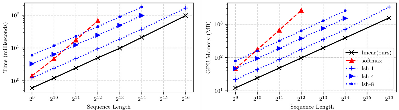
Figure 1: Comparison of the computational requirements for a forward/backward pass for Reformer (lsh-X), softmax attention and linear attention. Linear and Reformer models scale linearly with the sequence length unlike softmax which scales with the square of the sequence length both in memory and time. Full details of the experiment can be found in $\S4.1$ .
图 1: Reformer (lsh-X)、softmax注意力机制与线性注意力机制在前向/反向传播中的计算需求对比。与按序列长度平方级增长内存和时间消耗的softmax不同,线性模型和Reformer模型的消耗随序列长度线性增长。实验完整细节详见$\S4.1$。

Figure 2: Convergence comparison of softmax, linear and reformer attention on a sequence duplication task. linear converges stably and reaches the same final performance as softmax. The details of the experiment are in $\S4.1$ .
图 2: 序列复制任务中softmax、linear和reformer注意力的收敛对比。linear稳定收敛并达到与softmax相同的最终性能。实验细节见 $\S4.1$。
4.1.2. MEMORY AND COMPUTATIONAL REQUIREMENTS
4.1.2. 内存与计算需求
In this subsection, we compare transformers with respect to their computational and memory requirements. We compute the attention and the gradients for a synthetic input with varying sequence lengths $N\in{2^{9},2^{10},\dots,2^{16}}$ and measure the peak allocated GPU memory and required time for each variation of transformer. We scale the batch size inversely with the sequence length and report the time and memory per sample in the batch.
在本小节中,我们比较了不同Transformer模型在计算和内存需求方面的表现。针对合成输入数据,我们计算了注意力机制和梯度,其中序列长度变化范围为$N\in{2^{9},2^{10},\dots,2^{16}}$,并测量了每种Transformer变体的GPU峰值内存分配及计算耗时。实验采用批量大小与序列长度成反比的缩放策略,最终汇报批次中每个样本的时间和内存消耗。
Every method is evaluated up to the maximum sequence length that fits the GPU memory. For this benchmark we use an NVidia GTX 1080 Ti with 11GB of memory. This results in a maximum sequence length of 4,096 elements for softmax and 16,384 for lsh-4 and lsh-8. As expected, softmax scales quadratically with respect to the sequence length. Our method is faster and requires less memory than the baselines for every configuration, as seen in figure 1. We observe that both Reformer and linear attention scale linearly with the sequence length. Note that although the asymptotic complexity for Reformer is $\mathcal{O}\left(N\log N\right)$ , $\log N$ is small enough and does not affect the computation time.
每种方法都在不超过GPU显存的最大序列长度下进行评估。本基准测试使用配备11GB显存的NVidia GTX 1080 Ti显卡。结果显示,softmax的最大序列长度为4,096个元素,而lsh-4和lsh-8则达到16,384。如预期所示,softmax的计算复杂度随序列长度呈平方级增长。如图1所示,我们的方法在所有配置下都比基线方案更快且内存占用更低。我们观察到Reformer和线性注意力机制的计算复杂度均与序列长度呈线性关系。需要注意的是,尽管Reformer的渐进复杂度为$\mathcal{O}\left(N\log N\right)$,但$\log N$值足够小,不会显著影响计算时间。
4.2. Image Generation
4.2. 图像生成
Transformers have shown great results on the task of conditional or unconditional auto regressive generation (Radford et al., 2019; Child et al., 2019), however, sampling from transformers is slow due to the task being inherently sequential and the memory scaling with the square of the sequence length. In this section, we train causally masked transformers to predict images pixel by pixel. Our achieved performance in terms of bits per dimension is on par with softmax attention while being able to generate images more than 1,000 times faster and with constant memory per image from the first to the last pixel. We refer the reader to our supplementary for comparisons in terms of training evolution, quality of generated images and time to generate a single image. In addition, we also compare with a faster softmax transformer that caches the keys and values during inference, in contrast to the PyTorch implementation.
Transformer 在条件或无条件自回归生成任务中表现出色 (Radford et al., 2019; Child et al., 2019) ,但由于任务本身具有序列性且内存随序列长度平方级增长,从 Transformer 中采样速度较慢。本节我们训练因果掩码 Transformer 逐像素预测图像。在每维度比特数指标上,我们的表现与 softmax 注意力机制相当,同时能以超过 1,000 倍的速度生成图像,且从首像素到尾像素保持恒定的单图内存占用。训练过程演变、生成图像质量和单图生成时间的对比详见补充材料。此外,我们还对比了推理时缓存键值的快速 softmax Transformer 与 PyTorch 实现方案。
4.2.1. MNIST
4.2.1. MNIST
First, we evaluate our model on image generation with auto regressive transformers on the widely used MNIST dataset (LeCun et al., 2010). The architecture for this experiment comprises 8 attention layers with 8 attention heads each. We set the embedding size to 256 which is 32 dimensions per head. Our feed forward dimensions are 4 times larger than our embedding size. We model the output with a mixture of 10 logistics as introduced by Salimans et al. (2017). We use the RAdam optimizer with a learning rate of $10^{-4}$ and train all models for 250 epochs. For the reformer baseline, we use 1 and 4 hashing rounds. Furthermore, as suggested in Kitaev et al. (2020), we use 64 buckets and chunks with approximately 32 elements. In particular, we divide the 783 long input sequence to 27 chunks of 29 elements each. Since the sequence length is realtively small, namely only 784 pixels, to remove differences due to different batch sizes we use a batch size of 10 for all methods.
首先,我们在广泛使用的MNIST数据集(LeCun等人,2010)上通过自回归Transformer评估了我们的图像生成模型。该实验的架构包含8个注意力层,每层有8个注意力头。我们将嵌入大小设置为256,即每个头32维。前馈网络的维度是嵌入大小的4倍。我们采用Salimans等人(2017)提出的10个logistic混合来建模输出。使用学习率为$10^{-4}$的RAdam优化器,所有模型均训练250个epoch。对于Reformer基线模型,我们采用1轮和4轮哈希处理。此外,按照Kitaev等人(2020)的建议,我们使用64个桶和约含32个元素的块。具体而言,我们将783长的输入序列划分为27个块,每块含29个元素。由于序列长度相对较小(仅784像素),为消除不同批量大小带来的差异,所有方法均采用批量大小为10。
Table 1: Comparison of auto regressive image generation of MNIST images. Our linear transformers achieve almost the same bits/dim as the full softmax attention but more than 300 times higher throughput in image generation. The full details of the experiment are in $\S4.2.1$ .
| Method | Bits/dim | Images/sec |
| Softmax | 0.621 | 0.45 (1×) |
| LSH-1 | 0.745 | 0.68 (1.5×) |
| LSH-4 | 0.676 | 0.27 (0.6×) |
| Linear (ours) | 0.644 | 142.8 (317×) |
表 1: MNIST图像自回归生成的对比。我们的线性Transformer在图像生成中实现了与完整softmax注意力几乎相同的bits/dim,但吞吐量提高了300多倍。实验细节详见$\S4.2.1$。
| 方法 | Bits/dim | 图像/秒 |
|---|---|---|
| Softmax | 0.621 | 0.45 (1×) |
| LSH-1 | 0.745 | 0.68 (1.5×) |
| LSH-4 | 0.676 | 0.27 (0.6×) |
| Linear (ours) | 0.644 | 142.8 (317×) |
Table 1 summarizes the results. We observe that linear transformers achieve almost the same performance, in terms of final perplexity, as softmax transformers while being able to generate images more than 300 times faster. This is achieved due to the low memory requirements of our model, which is able to simultaneously generate 10,000 MNIST images with a single GPU. In particular, the memory is constant with respect to the sequence length because the only thing that needs to be stored between pixels are the $s_ {i}$ and $z_ {i}$ values as described in equations 18 and 19. On the other hand, both softmax and Reformer require memory that increases with the length of the sequence.
表 1: 总结了实验结果。我们观察到,线性 Transformer 在最终困惑度指标上与 softmax Transformer 表现几乎相当,同时图像生成速度提升超过 300 倍。这一优势源于我们模型的低内存需求——单块 GPU 即可同时生成 10,000 张 MNIST 图像。具体而言,由于只需按公式 (18) 和 (19) 存储像素间的 $s_ {i}$ 和 $z_ {i}$ 值,模型内存消耗与序列长度无关。相比之下,softmax 和 Reformer 的内存需求会随序列长度增长而增加。
Image completions and unconditional samples from our MNIST model can be seen in figure 3. We observe that our linear transformer generates very convincing samples with sharp boundaries and no noise. In the case of image completion, we also observe that the transformer learns to use the same stroke style and width as the original image effectively attending over long temporal distances. Note that as the achieved perplexity is more or less the same for all models, we do not observe qualitative differences between the generated samples from different models.
图3展示了我们MNIST模型的图像补全和无条件生成样本。观察到线性Transformer生成的样本具有清晰边界且无噪点,效果极具说服力。在图像补全任务中,该Transformer还能有效学习原图的笔触风格与线条宽度,实现了长时程的精准注意力建模。需要注意的是,由于所有模型的困惑度表现相近,不同模型生成的样本在质量上未见显著差异。
4.2.2. CIFAR-10
4.2.2. CIFAR-10
The benefits of our linear formulation increase as the sequence length increases. To showcase that, we train 16 layer transformers to generate CIFAR-10 images (Krizhevsky et al., 2009). For each layer we use the same configuration as in the previous experiment. For Reformer, we use again 64 buckets and 83 chunks of 37 elements, which is approximately 32, as suggested in the paper. Since the sequence length is almost 4 times larger than for the previous experiment, the full transformer can only be used with a batch size of 1 in the largest GPU that is available to us, namely an NVidia P40 with 24GB of memory. For both the linear transformer and reformer, we use a batch size of 4. All models are trained for 7 days. We report results in terms of bits per dimension and image generation throughput in table 2. Note that although the main point of this experiment is not the final perplexity, it is evident that as the sequence length grows, the fast transformer models become increasingly more efficient per GPU hour, achieving better scores than their slower counterparts.
我们的线性公式优势随着序列长度的增加而增强。为展示这一点,我们训练了16层Transformer来生成CIFAR-10图像 (Krizhevsky et al., 2009)。每层采用与前次实验相同的配置。对于Reformer,我们再次使用64个桶和83个含37元素的块(约32个),如原论文建议。由于序列长度比前次实验大近4倍,完整Transformer只能在现有最大GPU(24GB显存的NVidia P40)上以批处理大小1运行。线性Transformer和Reformer均采用批处理大小4。所有模型训练7天。表2展示了每维度比特数和图像生成吞吐量的结果。需注意,虽然本实验重点不在最终困惑度,但明显可见:随着序列增长,快速Transformer模型在每GPU小时效率上持续提升,其表现优于速度较慢的对应模型。
表2:
Table 2: We train auto regressive transformers for 1 week on a single GPU to generate CIFAR-10 images. Our linear transformer completes 3 times more epochs than softmax, which results in better perplexity. Our model generates images $4\small{,}000\times$ faster than the baselines. The full details of the experiment are in $\S4.2.2$ .
| Method | Bits/dim | Images/sec |
| Softmax | 3.47 | 0.004 (1×) |
| LSH-1 | 3.39 | 0.015 (3.75×) |
| LSH-4 | 3.51 | 0.005 (1.25×) |
| Linear (ours) | 3.40 | 17.85 (4,462×) |
表 2: 我们在单个GPU上用自回归Transformer训练1周来生成CIFAR-10图像。我们的线性Transformer完成的训练轮次是softmax的3倍,从而获得了更好的困惑度。我们的模型生成图像速度比基线快 $4\small{,}000\times$ 。完整实验细节见 $\S4.2.2$ 。
| 方法 | 比特/维度 | 图像/秒 |
|---|---|---|
| Softmax | 3.47 | 0.004 (1×) |
| LSH-1 | 3.39 | 0.015 (3.75×) |
| LSH-4 | 3.51 | 0.005 (1.25×) |
| Linear (ours) | 3.40 | 17.85 (4,462×) |
As the memory and time to generate a single pixel scales quadratically with the number of pixels for both Reformer and softmax attention, the increase in throughput for our linear transformer is even more pronounced. In particular, for every image generated by the softmax transformer, our method can generate 4,460 images. Image completions and unconditional samples from our model can be seen in figure 4. We observe that our model generates images with spatial consistency and can complete images con vinci gly without significantly hindering the recognition of the image category. For instance, in figure 4b, all images have successfully completed the dog’s nose (first row) or the windshield of the truck (last row).
由于Reformer和softmax注意力生成单个像素所需的内存和时间与像素数量呈平方关系,我们的线性Transformer在吞吐量上的提升更为显著。具体而言,softmax Transformer每生成1张图像,我们的方法可生成4,460张图像。图4展示了我们模型的图像补全和无条件生成样本。我们观察到,该模型生成的图像具有空间一致性,并能流畅地完成图像补全,同时不会显著影响图像类别的识别。例如在图4b中,所有图像都成功补全了狗的鼻子(第一行)或卡车的挡风玻璃(最后行)。
4.3. Automatic Speech Recognition
4.3. 自动语音识别
To show that our method can also be used for nonauto regressive tasks, we evaluate the performance of linear transformers in end-to-end automatic speech recognition using Connection is t Temporal Classification (CTC) loss (Graves et al., 2006). In this setup, we predict a distribution over phonemes for each input frame in a non autore- gressive fashion. We use the 80 hour WSJ dataset (Paul & Baker, 1992) with 40-dimensional mel-scale filter banks without temporal differences as features. The dataset contains sequences with 800 frames on average and a maximum sequence length of 2,400 frames. For this task, we also compare with a bidirectional LSTM (Hochreiter & Schmid huber, 1997) with 3 layers of hidden size 320. We use the Adam optimizer (Kingma & Ba, 2014) with a learning rate of $10^{-3}$ which is reduced when the validation error stops decreasing. For the transformer models, we use 9 layers with 6 heads with the same embedding dimensions as for the image experiments. As an optimizer, we use RAdam with an initial learning rate of $10^{-4}$ that is divided by 2 when the validation error stops decreasing.
为证明我们的方法同样适用于非自回归任务,我们在线性Transformer上使用连接时序分类(CTC)损失[Graves等人,2006]评估端到端自动语音识别性能。该任务以非自回归方式为每个输入帧预测音素分布。我们采用80小时WSJ数据集[Paul & Baker,1992],使用40维梅尔尺度滤波器组(不含时序差分)作为特征。数据集平均序列长度为800帧,最大序列长度2,400帧。对比基线为3层隐层维度320的双向LSTM[Hochreiter & Schmidhuber,1997],使用Adam优化器[Kingma & Ba,2014],初始学习率$10^{-3}$并在验证误差停滞时降低。Transformer模型采用9层6头结构,嵌入维度与图像实验保持一致,使用初始学习率$10^{-4}$的RAdam优化器,验证误差停滞时学习率减半。

Figure 3: Unconditional samples and image completions generated by our method for MNIST. (a) depicts the occluded orignal images, (b) the completions and (c) the original. Our model achieves comparable bits/dimension to softmax, while having more than 300 times higher throughput, generating 142 images/second. For details see $\S4.2.1$ . Figure 4: Unconditional samples and image completions generated by our method for CIFAR-10. (a) depicts the occluded orignal images, (b) the completions and (c) the original. As the sequence length grows linear transformers become more efficient compared to softmax attention. Our model achieves more than 4,000 times higher throughput and generates 17.85 images/second. For details see $\S4.2.2$ .
图 3: 我们的方法在MNIST上生成的无条件样本及图像补全结果。(a) 为遮挡后的原始图像,(b) 为补全结果,(c) 为原始图像。我们的模型在bits/dimension指标上与softmax相当,同时吞吐量提升300倍以上,生成速度达142张/秒。详见$\S4.2.1$。
图 4: 我们的方法在CIFAR-10上生成的无条件样本及图像补全结果。(a) 为遮挡后的原始图像,(b) 为补全结果,(c) 为原始图像。随着序列长度增加,线性Transformer相比softmax注意力机制效率优势更显著。我们的模型吞吐量提升超4,000倍,生成速度达17.85张/秒。详见$\S4.2.2$。
Table 3: Performance comparison in automatic speech recognition on the WSJ dataset. The results are given in the form of phoneme error rate (PER) and training time per epoch. Our model outperforms the LSTM and Reformer while being faster to train and evaluate. Details of the experiment can be found in $\S4.3$ .
| Method | ValidationPER | Time/epoch (s) |
| Bi-LSTM | 10.94 | 1047 |
| Softmax | 5.12 | 2711 |
| LSH-4 | 9.33 | 2250 |
| Linear (ours) | 8.08 | 824 |
表 3: WSJ数据集上自动语音识别的性能对比。结果以音素错误率(PER)和每轮训练时间呈现。我们的模型在训练和评估速度更快的同时,性能优于LSTM和Reformer。实验细节详见$\S4.3$。
| 方法 | 验证集PER | 每轮时间(s) |
|---|---|---|
| Bi-LSTM | 10.94 | 1047 |
| Softmax | 5.12 | 2711 |
| LSH-4 | 9.33 | 2250 |
| Linear(ours) | 8.08 | 824 |
All models are evaluated in terms of phoneme error rate (PER) and training time per epoch. We observe that linear outperforms the recurrent network baseline and Reformer both in terms of performance and speed by a large margin, as seen in table 3. Note that the softmax transformer, achieves lower phone error rate in comparison to all baselines, but is significantly slower. In particular, linear transformer is more than $3\times$ faster per epoch. We provide training evolution plots in the supplementary.
所有模型均以音素错误率(PER)和每轮训练时间为评估指标。如表3所示,线性模型在性能和速度上均显著优于循环网络基线及Reformer。值得注意的是,softmax transformer虽然比所有基线模型获得更低的音素错误率,但训练速度明显更慢。具体而言,线性transformer每轮训练速度提升超过$3\times$倍。训练过程曲线图详见补充材料。
5. Conclusions
5. 结论
In this work, we presented linear transformer, a model that significantly reduces the memory and computational cost of the original transformers. In particular, by exploiting the associativity property of matrix products we are able to compute the self-attention in time and memory that scales linearly with respect to the sequence length. We show that our model can be used with causal masking and still retain its linear asymptotic complexities. Finally, we express the transformer model as a recurrent neural network, which allows us to perform inference on auto regressive tasks thousands of time faster.
在这项工作中,我们提出了线性Transformer (linear transformer) ,该模型显著降低了原始Transformer的内存和计算成本。具体而言,通过利用矩阵乘法的结合性特性,我们能够以与序列长度呈线性关系的时间和内存来计算自注意力 (self-attention) 。我们证明了该模型可与因果掩码 (causal masking) 结合使用,同时仍保持其线性渐近复杂度。最后,我们将Transformer模型表示为循环神经网络 (RNN) ,这使得我们能够以快数千倍的速度执行自回归 (auto regressive) 任务的推理。
This property opens a multitude of directions for future research regarding the storage and retrieval of information in both RNNs and transformers. Another line of research to be explored is related to the choice of feature map for linear attention. For instance, approximating the RBF kernel with random Fourier features could allow us to use models pretrained with softmax attention.
这一特性为RNN和Transformer中的信息存储与检索研究开辟了众多方向。另一个待探索的研究方向涉及线性注意力特征图的选择。例如,通过随机傅里叶特征逼近RBF核函数,可能使我们能够利用基于softmax注意力预训练的模型。
Acknowledgements
致谢
Angelos Katha ro poul os was supported by the Swiss National Science Foundation under grant numbers FNS-30209 ”ISUL” and FNS-30224 ”CORTI”. Apoorv Vyas was sup- ported by the Swiss National Science Foundation under grant number FNS-30213 ”SHISSM”. Nikolaos Pappas was supported by the Swiss National Science Foundation under grant number P400P2 183911 ”UNISON”.
Angelos Katharopoulos 由瑞士国家科学基金会资助,项目编号为 FNS-30209 "ISUL" 和 FNS-30224 "CORTI"。
Apoorv Vyas 由瑞士国家科学基金会资助,项目编号为 FNS-30213 "SHISSM"。
Nikolaos Pappas 由瑞士国家科学基金会资助,项目编号为 P400P2 183911 "UNISON"。
References
参考文献
Morin, F. and Bengio, Y. Hierarchical probabilistic neural network language model. In Aistats, volume 5, pp. 246– 252. Citeseer, 2005.
Morin, F. 和 Bengio, Y. 分层概率神经网络语言模型。见《Aistats》第5卷,第246-252页。Citeseer,2005年。
ference of the International Speech Communication Association (Inter Speech 2018), Hyderabad, India, September 2018.
国际语音通信协会会议(Inter Speech 2018),印度海得拉巴,2018年9月。
Supplementary Material for Transformers are RNNs: Fast Auto regressive Transformers with Linear Attention
Transformer 是 RNN:线性注意力快速自回归 Transformer 的补充材料
A. Gradient Derivation
A. 梯度推导
In the first section of our supplementary material, we derive in detail the gradients for causally masked linear transformers and show that they can be computed in linear time and constant memory. In particular, we derive the gradients of a scalar loss with respect to the numerator of the following equation,
在我们补充材料的第一部分,我们详细推导了因果掩码线性Transformer的梯度,并证明它们可以在线性时间和恒定内存下计算。具体而言,我们推导了标量损失相对于下式分子的梯度:
$$
V_ {i}^{\prime}=\frac{\phi\left(Q_ {i}\right)^{T}\sum_ {j=1}^{i}\phi\left(K_ {j}\right)V_ {j}^{T}}{\phi\left(Q_ {i}\right)^{T}\sum_ {j=1}^{i}\phi\left(K_ {j}\right)}.
$$
$$
V_ {i}^{\prime}=\frac{\phi\left(Q_ {i}\right)^{T}\sum_ {j=1}^{i}\phi\left(K_ {j}\right)V_ {j}^{T}}{\phi\left(Q_ {i}\right)^{T}\sum_ {j=1}^{i}\phi\left(K_ {j}\right)}.
$$
The gradient with respect to the denominator and the fraction are efficiently handled by autograd. Without loss of generality, we can assume that $Q$ and $K$ already contain the vectors mapped by $\phi\left(\cdot\right)$ , hence given the numerator
分母和分数的梯度由自动微分 (autograd) 高效处理。不失一般性,我们可以假设 $Q$ 和 $K$ 已包含通过 $\phi\left(\cdot\right)$ 映射的向量,因此给定分子
$$
\bar{V}_ {i}=Q_ {i}^{T}\sum_ {j=1}^{i}K_ {j}V_ {j}^{T},
$$
$$
\bar{V}_ {i}=Q_ {i}^{T}\sum_ {j=1}^{i}K_ {j}V_ {j}^{T},
$$
and $\nabla_ {\bar{V}}{\mathcal{L}}$ we seek to compute $\nabla_ {Q}\mathcal{L},\nabla_ {K}\mathcal{L}$ and $\nabla_ {V}{\mathcal{L}}$ . Note that $Q\in\mathbb{R}^{N\times D}$ , ${\cal K}\in\mathbb{R}^{N\times D}$ and $V\in\mathbb{R}^{N\times M}$ . To derive the gradients, we first express the above equation for a single element without using vector notation,
以及 $\nabla_ {\bar{V}}{\mathcal{L}}$,我们需要计算 $\nabla_ {Q}\mathcal{L}$、$\nabla_ {K}\mathcal{L}$ 和 $\nabla_ {V}{\mathcal{L}}$。注意 $Q\in\mathbb{R}^{N\times D}$、${\cal K}\in\mathbb{R}^{N\times D}$ 和 $V\in\mathbb{R}^{N\times M}$。为了推导梯度,我们首先用标量形式表示上述方程(不使用向量符号):
$$
\bar{V}_ {i e}=\sum_ {d=1}^{D}Q_ {i d}\sum_ {j=1}^{i}K_ {j d}V_ {j e}=\sum_ {d=1}^{D}\sum_ {j=1}^{i}Q_ {i d}K_ {j d}V_ {j e}.
$$
$$
\bar{V}_ {i e}=\sum_ {d=1}^{D}Q_ {i d}\sum_ {j=1}^{i}K_ {j d}V_ {j e}=\sum_ {d=1}^{D}\sum_ {j=1}^{i}Q_ {i d}K_ {j d}V_ {j e}.
$$
Subsequently we can start deriving the gradients for $Q$ by taking the partial derivative for any $Q_ {l t}$ , as follows
随后我们可以开始推导 $Q$ 的梯度,即对任意 $Q_ {l t}$ 求偏导,如下所示
$$
\frac{\partial\mathcal{L}}{\partial Q_ {l t}}=\sum_ {e=1}^{M}\frac{\partial\mathcal{L}}{\partial\bar{V}_ {l e}}\frac{\partial\bar{V}_ {l e}}{\partial Q_ {l t}}=\sum_ {e=1}^{M}\frac{\partial\mathcal{L}}{\partial\bar{V}_ {l e}}\left(\sum_ {j=1}^{l}K_ {j t}V_ {j e}\right).
$$
$$
\frac{\partial\mathcal{L}}{\partial Q_ {l t}}=\sum_ {e=1}^{M}\frac{\partial\mathcal{L}}{\partial\bar{V}_ {l e}}\frac{\partial\bar{V}_ {l e}}{\partial Q_ {l t}}=\sum_ {e=1}^{M}\frac{\partial\mathcal{L}}{\partial\bar{V}_ {l e}}\left(\sum_ {j=1}^{l}K_ {j t}V_ {j e}\right).
$$
If we write the above equation as a matrix product of gradients it becomes,
若我们将上述方程写作梯度的矩阵乘积形式,则可得:
$$
\nabla_ {Q_ {i}}\mathcal{L}=\nabla_ {\bar{V}_ {i}}\mathcal{L}\left(\sum_ {j=1}^{i}K_ {j}V_ {j}^{T}\right)^{T},
$$
$$
\nabla_ {Q_ {i}}\mathcal{L}=\nabla_ {\bar{V}_ {i}}\mathcal{L}\left(\sum_ {j=1}^{i}K_ {j}V_ {j}^{T}\right)^{T},
$$
proving equation 13 from the main paper. In equation 24 we made use of the fact that $Q_ {l t}$ only affects $\bar{V_ {l}}$ hence we do not need to sum over $i$ to compute the gradients. However, for $K$ and $V$ this is not the case. In particular, $K_ {j}$ affects all $\bar{V_ {i}}$ where $i\geq j$ . Consequently, we can write the partial derivative of the loss with respect to $K_ {l t}$ as follows,
证明主论文中的公式13。在公式24中,我们利用了$Q_ {l t}$仅影响$\bar{V_ {l}}$这一事实,因此不需要对$i$求和来计算梯度。然而,对于$K$和$V$则并非如此。具体而言,$K_ {j}$会影响所有$i\geq j$的$\bar{V_ {i}}$。因此,我们可以将损失函数对$K_ {l t}$的偏导数表示如下:
$$
\begin{array}{r l}&{\displaystyle\frac{\partial\mathcal{L}}{\partial K_ {l t}}=\sum_ {e=1}^{M}\sum_ {i=l}^{N}\frac{\partial\mathcal{L}}{\partial\bar{V}_ {i e}}\frac{\partial\bar{V}_ {i e}}{\partial K_ {l t}}=\sum_ {e=1}^{M}\sum_ {i=l}^{N}\frac{\partial\mathcal{L}}{\partial\bar{V}_ {i e}}\frac{\partial\left(\sum_ {d=1}^{D}\sum_ {j=1}^{i}Q_ {i d}K_ {j d}V_ {j e}\right)}{\partial K_ {l t}}}\ &{\quad\quad\quad\quad\quad=\sum_ {e=1}^{M}\sum_ {i=l}^{N}\frac{\partial\mathcal{L}}{\partial\bar{V}_ {i e}}Q_ {i t}V_ {l e}.}\end{array}
$$
$$
\begin{array}{r l}&{\displaystyle\frac{\partial\mathcal{L}}{\partial K_ {l t}}=\sum_ {e=1}^{M}\sum_ {i=l}^{N}\frac{\partial\mathcal{L}}{\partial\bar{V}_ {i e}}\frac{\partial\bar{V}_ {i e}}{\partial K_ {l t}}=\sum_ {e=1}^{M}\sum_ {i=l}^{N}\frac{\partial\mathcal{L}}{\partial\bar{V}_ {i e}}\frac{\partial\left(\sum_ {d=1}^{D}\sum_ {j=1}^{i}Q_ {i d}K_ {j d}V_ {j e}\right)}{\partial K_ {l t}}}\ &{\quad\quad\quad\quad\quad=\sum_ {e=1}^{M}\sum_ {i=l}^{N}\frac{\partial\mathcal{L}}{\partial\bar{V}_ {i e}}Q_ {i t}V_ {l e}.}\end{array}
$$
As for $Q$ we can now write the gradient in vectorized form,
至于 $Q$,我们现在可以用向量化形式写出梯度,
$$
\nabla_ {K_ {i}}\mathcal{L}=\left(\sum_ {j=i}^{N}Q_ {j}\left(\nabla_ {\bar{V}_ {j}}\mathcal{L}\right)^{T}\right)V_ {i},
$$
$$
\nabla_ {K_ {i}}\mathcal{L}=\left(\sum_ {j=i}^{N}Q_ {j}\left(\nabla_ {\bar{V}_ {j}}\mathcal{L}\right)^{T}\right)V_ {i},
$$
proving equation 14 from the paper. Following the same reasoning, we can compute the partial derivative of the loss with respect to $V_ {l t}$ and prove equation 15. Note that the cumulative sum matrices for the gradient with respect to $Q$ and $K$ have the same size, however one is computed in the forward direction (summing from 1 to $N$ ) similarly to the forward pass and the other is computed in the backwards direction (summing from $N$ to 1) similar to back propagation through time done in RNNs.
根据论文证明公式14。同理,我们可以计算损失对$V_ {lt}$的偏导数并证明公式15。需注意,关于$Q$和$K$的梯度累积求和矩阵尺寸相同,但一个是正向计算(从1到$N$求和)类似于前向传播,另一个是反向计算(从$N$到1求和)类似于RNN中的时间反向传播。
B. Training Evolution
B. 训练演进
In figure 5 we present the training evolution of all transformer models in our experiments. For the MNIST experiment (Fig. 5a) we train all methods for 250 epochs. The sequence length is small enough so that the training time does not vary significantly for all methods. We observe that our method converges on par with softmax attention outperforming significantly both reformer variants.
在图5中,我们展示了实验中所有Transformer模型的训练演变过程。对于MNIST实验(图5a),所有方法均训练250个周期。由于序列长度足够小,各方法的训练时间差异不大。我们观察到,本文方法的收敛速度与softmax注意力相当,且显著优于两种reformer变体。
On the other hand, for CIFAR-10 (Fig. 5b) we train all methods for a fixed amount of time, namely 7 days. We observe that lsh-1 and linear complete significantly more epochs than softmax and lsh-4 and achieve better performance. This gap is expected to increase with a further increase in sequence length.
另一方面,对于CIFAR-10 (图 5b) ,我们将所有方法的训练时间固定为7天。观察到 lsh-1 和 linear 比 softmax 和 lsh-4 完成了更多轮次,并取得了更好的性能。随着序列长度的进一步增加,这一差距预计会扩大。
Finally, in our last experiment on automatic speech recognition (Fig. 5c), softmax outperforms significantly both Reformer and linear in terms of convergence. Note that linear is $3\times$ faster per epoch which means it has completed approximately 4 times more epochs in comparison to softmax. Even though softmax attention is better in this task, we observe that linear transformers significantly outperform Reformer both in terms of convergence and final performance.
最后,在我们关于自动语音识别 (automatic speech recognition) 的最后一项实验中 (图 5c),softmax 在收敛性方面显著优于 Reformer 和 linear。需要注意的是,linear 每轮训练速度快 $3\times$,这意味着它比 softmax 多完成了大约 4 倍的训练轮次。尽管 softmax attention 在此任务中表现更优,但我们观察到 linear transformers 在收敛性和最终性能上都显著优于 Reformer。

Figure 5: Training evolution of transformers for all our experiments. It can be observed that linear transformers converge consistently faster than Reformer and in the auto regressive experiments on par with softmax. For MNIST all methods are trained for 250 epochs while for CIFAR we train for 7 days. In the speech recognition experiments all methods are trained to convergence. The details of the experiments can be found in $\S4.2.1$ , $\S4.2.2$ and $\S4.3$ in the main paper.
图 5: 所有实验中Transformer的训练演变过程。可以观察到,线性Transformer的收敛速度始终快于Reformer,在自回归实验中与softmax表现相当。MNIST实验中所有方法均训练250轮,而CIFAR实验持续训练7天。语音识别实验中所有方法均训练至收敛。实验细节详见主论文中的$\S4.2.1$、$\S4.2.2$和$\S4.3$章节。
C. Image Generation Throughput Discussion
C. 图像生成吞吐量讨论
C.1. Stateful softmax attention
C.1. 有状态软注意力机制 (Stateful softmax attention)
In $\S4.2$ of the main paper, we report the image generation throughput and we compare with softmax transformer and lsh. In this section we create another baseline, denoted as stateful-softmax, that implements a softmax auto regressive transformer as a recurrent model. Namely, all the keys and values are saved and then passed to the model again when predicting the next element of the sequence. The state of this recurrent model is the set of keys and values which has size proportional to the sequence length. This is qualitatively different to our proposed model that has a state with fixed dimensions and computing the $i$ -th state given the previous one has fixed computational cost regardless of $i$ .
在论文主体部分的 $\S4.2$ 中,我们报告了图像生成吞吐量,并与softmax transformer和LSH进行了对比。本节我们建立了另一个基线模型,称为stateful-softmax,它将softmax自回归transformer实现为循环模型。具体而言,所有键(key)和值(value)都会被保存,并在预测序列下一个元素时再次传递给模型。该循环模型的状态是键值集合,其大小与序列长度成正比。这与我们提出的模型存在本质差异:我们的模型具有固定维度的状态,且计算第 $i$ 个状态时(给定前一个状态)的计算成本是固定的,与 $i$ 无关。
Table 4 summarizes the results. We observe that stateful-softmax is significantly faster than vanilla transformers. However, its complexity is still quadratic with respect to the sequence length and our for uml ation is more than $50\times$ faster for CIFAR-10. Moreover, we would like to point out that implementing a similar stateful attention for Reformer is not a trivial task as the sorting and chunking operations need to be performed each time a new input is provided.
表 4 总结了实验结果。我们发现 stateful-softmax 比传统 Transformer 快得多,但其复杂度仍与序列长度呈平方关系。在 CIFAR-10 数据集上,我们的方法实现了超过 $50\times$ 的加速比。此外需要指出,为 Reformer 实现类似的状态化注意力机制并非易事,因为每次接收新输入时都需要重新执行排序和分块操作。
Transformers are RNNs
| Method | Bits/dim | Images/sec |
| Softmax | 0.621 | 0.45 (1×) |
| Stateful-softmax | 0.621 | 7.56 (16.8×) |
| LSH-1 | 0.745 | 0.68 (1.5×) |
| LSH-4 | 0.676 | 0.27 (0.6×) |
| Linear (ours) | 0.644 | 142.8 (317×) |
Transformer 是循环神经网络
| 方法 | 比特/维度 | 图像/秒 |
|---|---|---|
| Softmax | 0.621 | 0.45 (1×) |
| Stateful-softmax | 0.621 | 7.56 (16.8×) |
| LSH-1 | 0.745 | 0.68 (1.5×) |
| LSH-4 | 0.676 | 0.27 (0.6×) |
| Linear (ours) | 0.644 | 142.8 (317×) |
(a) Image generation on MNIST
(a) 在MNIST数据集上的图像生成
(b) Image generation on CIFAR-10
| Method | Bits/dim | Images/sec |
| Softmax | 3.47 | 0.004 (1×) |
| Stateful-softmax | 3.47 | 0.32 (80×) |
| LSH-1 | 3.39 | 0.015 (3.75×) |
| LSH-4 | 3.51 | 0.005 (1.25×) |
| Linear (ours) | 3.40 | 17.85 (4,462×) |
(b) CIFAR-10 上的图像生成
| 方法 | Bits/dim | Images/sec |
|---|---|---|
| Softmax | 3.47 | 0.004 (1×) |
| Stateful-softmax | 3.47 | 0.32 (80×) |
| LSH-1 | 3.39 | 0.015 (3.75×) |
| LSH-4 | 3.51 | 0.005 (1.25×) |
| Linear (ours) | 3.40 | 17.85 (4,462×) |
Table 4: Comparison of auto regressive image generation throughput of MNIST and CIFAR-10 images. The experiment can be found in $\S4.2$ in the main paper. For stateful-softmax we save the keys and values and reuse them for predicting the next element. A detailed description of this extra baseline can be found in $\S\subset.1$ .
表 4: MNIST 和 CIFAR-10 图像自回归生成吞吐量对比。实验细节详见主论文 $\S4.2$ 。对于 stateful-softmax 方法,我们保存键值并复用于预测下一个元素。该额外基线的详细说明见 $\S\subset.1$ 。
C.2. Equalizing the batch size
C.2. 均衡批处理大小
In the previous sections we evaluate the throughput of all transformer variants for the task of auto regressive image generation. However, another important factor to consider is latency, namely the total time required to produce a single image. To this end, we use a batch size of 1 and measure the time required by all methods to generate a single image. In addition to running the inference on the GPU, we also evaluate the time required on CPU. The results are reported in table 5.
在前面的章节中,我们评估了所有Transformer变体在自回归图像生成任务中的吞吐量。然而,另一个需要考虑的重要因素是延迟,即生成单张图像所需的总时间。为此,我们使用批大小为1,并测量所有方法生成单张图像所需的时间。除了在GPU上运行推理外,我们还评估了在CPU上所需的时间。结果如表5所示。
(b) Image generation on CIFAR-10
| Method | Seconds (CPU) | Seconds (GPU) | Method | Seconds (CPU) | Seconds (GPU) | ||||
| Softmax | 72.6 | (13.2×) | 10.2 | (1.4×) | Softmax | 8651.4 | (191.8×) | 300.1 | (4.9×) |
| Stateful-softmax | 7.4 | (1.3×) | 10.4 | (1.42×) | Stateful-softmax | 71.9 | (1.6×) | 70.4 | (1.14×) |
| LSH-1 | 46.0 | (8.3×) | 19.2 | (2.6×) | LSH-1 | 2318.9 | (51.4x) | 221.6 | (3.6×) |
| LSH-4 | 112.0 | (20×) | 55.8 | (7.6×) | LSH-4 | 5263.7 | (116.7x) | 683.9 | (11.1x) |
| Linear (ours) | 5.5 | (1×) | 7.3 | (1×) | Linear (ours) | 45.1 | (1×) | 61.3 | (1×) |
(b) CIFAR-10 上的图像生成
| 方法 | 秒数 (CPU) | 秒数 (GPU) | 方法 | 秒数 (CPU) | 秒数 (GPU) | ||||
|---|---|---|---|---|---|---|---|---|---|
| Softmax | 72.6 | (13.2×) | 10.2 | (1.4×) | Softmax | 8651.4 | (191.8×) | 300.1 | (4.9×) |
| Stateful-softmax | 7.4 | (1.3×) | 10.4 | (1.42×) | Stateful-softmax | 71.9 | (1.6×) | 70.4 | (1.14×) |
| LSH-1 | 46.0 | (8.3×) | 19.2 | (2.6×) | LSH-1 | 2318.9 | (51.4×) | 221.6 | (3.6×) |
| LSH-4 | 112.0 | (20×) | 55.8 | (7.6×) | LSH-4 | 5263.7 | (116.7×) | 683.9 | (11.1×) |
| Linear (ours) | 5.5 | (1×) | 7.3 | (1×) | Linear (ours) | 45.1 | (1×) | 61.3 | (1×) |
(a) Image generation on MNIST
(a) MNIST 图像生成
Table 5: Comparison of the time required to generate a single image with auto regressive transformers on MNIST and CIFAR-10. We run all methods with a batch size of 1 both on CPU and GPU and report the total time in seconds. For all numbers in the table, lower is better.
表 5: 在 MNIST 和 CIFAR-10 数据集上使用自回归 Transformer (auto regressive transformers) 生成单张图像所需时间的对比。所有方法均在 CPU 和 GPU 上以批次大小为 1 运行,并记录总时间(单位为秒)。表中所有数值均为越低越好。
We observe that all methods under utilize the GPU and achieve significantly smaller image generation throughput than the one shown in table 4. The proposed linear transformer is faster than all the methods and in particular it is almost $6.6\times$ faster than softmax transformers for generating an image on CIFAR-10. Note that our linear auto regressive transformer is the only method that is faster on the CPU than on the GPU in every case. This is due to the fact that computing the attention as an RNN has such a low cost that the main computational bottleneck becomes the inevitable outer loop over the sequence.
我们观察到所有方法都未能充分利用GPU,其图像生成吞吐量远低于表4所示数据。提出的线性Transformer在所有方法中最快,尤其在CIFAR-10数据集上生成图像时,比softmax Transformer快约$6.6\times$。值得注意的是,我们的线性自回归Transformer是唯一在所有情况下CPU速度均优于GPU的方法,这是因为将注意力计算作为RNN处理的成本极低,使得序列外部循环成为主要计算瓶颈。
D. Qualitative Results on Image Generation
D. 图像生成的定性结果
In this section we provide qualitative results for our image generation experiments. Since the perplexity of all models is approximately the same, as expected, the qualitative differences are not significant. A rather interesting observation however is that the Reformer models provide significantly fewer variations in their unconditional samples. Moreover, we observe that image completion is a significantly easier task than unconditional generation as all models perform significantly better.
在本节中,我们展示了图像生成实验的定性结果。由于所有模型的困惑度(perplexity)大致相同,预期的定性差异并不显著。然而一个相当有趣的发现是:Reformer模型在无条件生成样本中提供的变体明显更少。此外,我们观察到图像补全任务比无条件生成简单得多,所有模型在该任务上的表现都显著提升。

Figure 6: Unconditional samples from the transformer models trained with MNIST. See $\S4.2.1$ in the main paper.
图 6: 基于MNIST训练的Transformer模型生成的无条件样本。详见主论文 $\S4.2.1$ 章节。

Figure 7: MNIST digit completion from all trained models. See $\S4.2.1$ in the main paper.
图 7: 所有训练模型对MNIST数字的补全效果。详见主论文 $\S4.2.1$ 章节。

Figure 8: Unconditional samples from the transformer models trained with CIFAR-10. See $\S4.2.2$ in the main paper.
图 8: 使用 CIFAR-10 训练的 Transformer 模型生成的无条件样本。详见主论文 $\S4.2.2$ 章节。

Figure 9: CIFAR-10 image completions from all trained transformer models. See $\S4.2.2$ in the main paper.
图 9: 所有训练好的Transformer模型在CIFAR-10数据集上的图像补全效果。详见主论文 $\S4.2.2$ 章节。