Object-Centric Learning with Slot Attention

基于Slot Attention的物体中心学习

Francesco Locatello2,3,†,*, Dirk Weiss en born 1, Thomas Unter thin er 1, Aravindh Mahendran1, Georg Heigold1, Jakob Uszkoreit1, Alexey Do sov it ski y 1,‡, and Thomas Kipf1,‡,*

Francesco Locatello2,3,†,*, Dirk Weissenborn1, Thomas Unterthiner1, Aravindh Mahendran1, Georg Heigold1, Jakob Uszkoreit1, Alexey Dosovitskiy1,‡, and Thomas Kipf1,‡,*

1Google Research, Brain Team 2Dept. of Computer Science, ETH Zurich 3Max-Planck Institute for Intelligent Systems

1谷歌研究院，Brain团队 2苏黎世联邦理工学院计算机科学系 3马克斯·普朗克智能系统研究所

Abstract

摘要

Learning object-centric representations of complex scenes is a promising step towards enabling efficient abstract reasoning from low-level perceptual features. Yet, most deep learning approaches learn distributed representations that do not capture the compositional properties of natural scenes. In this paper, we present the Slot Attention module, an architectural component that interfaces with perceptual representations such as the output of a convolutional neural network and produces a set of task-dependent abstract representations which we call slots. These slots are exchangeable and can bind to any object in the input by specializing through a competitive procedure over multiple rounds of attention. We empirically demonstrate that Slot Attention can extract object-centric representations that enable generalization to unseen compositions when trained on unsupervised object discovery and supervised property prediction tasks.

学习以物体为中心的复杂场景表示，是实现从低层次感知特征进行高效抽象推理的重要一步。然而，大多数深度学习方法学习的是分布式表示，无法捕捉自然场景的组合特性。本文提出Slot Attention模块，这一架构组件可与卷积神经网络输出等感知表示对接，并生成一组任务相关的抽象表示（我们称之为slot）。这些slot具有可交换性，通过多轮注意力竞争机制可动态绑定输入中的任意对象。实验表明，当用于无监督物体发现和监督属性预测任务时，Slot Attention提取的物体中心表示能够泛化至未见过的组合场景。

1 Introduction

1 引言

Object-centric representations have the potential to improve sample efficiency and generalization of machine learning algorithms across a range of application domains, such as visual reasoning [1], modeling of structured environments [2], multi-agent modeling [3–5], and simulation of interacting physical systems [6–8]. Obtaining object-centric representations from raw perceptual input, such as an image or a video, is challenging and often requires either supervision [1, 3, 9, 10] or task-specific architectures [2, 11]. As a result, the step of learning an object-centric representation is often skipped entirely. Instead, models are typically trained to operate on a structured representation of the environment that is obtained, for example, from the internal representation of a simulator [6, 8] or of a game engine [4, 5].

以对象为中心的表示方法有潜力提升机器学习算法在多个应用领域的样本效率和泛化能力，例如视觉推理[1]、结构化环境建模[2]、多智能体建模[3-5]以及交互物理系统仿真[6-8]。从原始感知输入(如图像或视频)中获取以对象为中心的表示具有挑战性，通常需要监督学习[1,3,9,10]或特定任务架构[2,11]。因此，学习以对象为中心的表示这一步骤经常被完全跳过。相反，模型通常被训练在从模拟器[6,8]或游戏引擎[4,5]内部表示获得的环境结构化表示上进行操作。

To overcome this challenge, we introduce the Slot Attention module, a differentiable interface between perceptual representations (e.g., the output of a CNN) and a set of variables called slots. Using an iterative attention mechanism, Slot Attention produces a set of output vectors with permutation symmetry. Unlike capsules used in Capsule Networks [12, 13], slots produced by Slot Attention do not specialize to one particular type or class of object, which could harm generalization. Instead, they act akin to object files [14], i.e., slots use a common representational format: each slot can store (and bind to) any object in the input. This allows Slot Attention to generalize in a systematic way to unseen compositions, more objects, and more slots.

为克服这一挑战，我们引入了Slot Attention模块，该模块在感知表征（如CNN的输出）与一组称为slot的变量之间建立了可微分接口。通过迭代注意力机制，Slot Attention生成具有排列对称性的输出向量集。与Capsule Networks[12,13]中使用的胶囊不同，Slot Attention生成的slot不会专用于特定类型或类别的对象（这可能损害泛化能力），而是类似于对象文件[14]：所有slot采用统一表征格式，每个slot可存储（并绑定）输入中的任意对象。这使得Slot Attention能以系统化方式泛化至未见过的组合、更多对象及更多slot。

Slot Attention is a simple and easy to implement architectural component that can be placed, for example, on top of a CNN [15] encoder to extract object representations from an image and is trained end-to-end with a downstream task. In this paper, we consider image reconstruction and set prediction as downstream tasks to showcase the versatility of our module both in a challenging unsupervised object discovery setup and in a supervised task involving set-structured object property prediction.

槽注意力 (Slot Attention) 是一种简单易实现的架构组件，例如可以放置在 CNN [15] 编码器之上，从图像中提取对象表征，并与下游任务进行端到端训练。在本文中，我们将图像重建和集合预测作为下游任务，以展示该模块在具有挑战性的无监督对象发现设置和涉及集合结构对象属性预测的监督任务中的多功能性。

Figure 1: (a) Slot Attention module and example applications to $(\mathbf{b})$ unsupervised object discovery and (c) supervised set prediction with labeled targets $y_ {i}$ . See main text for details.

图 1: (a) Slot Attention模块及其在 (b) 无监督物体发现和 (c) 带标注目标 $y_ {i}$ 的监督集合预测中的应用示例。详见正文。

Our main contributions are as follows: (i) We introduce the Slot Attention module, a simple architectural component at the interface between perceptual representations (such as the output of a CNN) and representations structured as a set. (ii) We apply a Slot Attention-based architecture to unsupervised object discovery, where it matches or outperforms relevant state-of-the-art approaches [16, 17], while being more memory efficient and significantly faster to train. (iii) We demonstrate that the Slot Attention module can be used for supervised object property prediction, where the attention mechanism learns to highlight individual objects without receiving direct supervision on object segmentation.

我们的主要贡献如下：(i) 我们引入了Slot Attention模块，这是一个位于感知表征(如CNN输出)与集合结构表征之间的简单架构组件。(ii) 我们将基于Slot Attention的架构应用于无监督物体发现任务，其性能匹配或超越相关前沿方法[16,17]，同时具有更高的内存效率和显著更快的训练速度。(iii) 我们证明Slot Attention模块可用于监督式物体属性预测，其注意力机制能在不接收物体分割直接监督的情况下学习突出单个物体。

2 Methods

2 方法

In this section, we introduce the Slot Attention module (Figure 1a; Section 2.1) and demonstrate how it can be integrated into an architecture for unsupervised object discovery (Figure 1b; Section 2.2) and into a set prediction architecture (Figure 1c; Section 2.3).

在本节中，我们将介绍Slot Attention模块(图1a；第2.1节)，并演示如何将其集成到无监督物体发现架构(图1b；第2.2节)和集合预测架构(图1c；第2.3节)中。

2.1 Slot Attention Module

2.1 槽注意力模块

The Slot Attention module (Figure 1a) maps from a set of $N$ input feature vectors to a set of $K$ output vectors that we refer to as slots. Each vector in this output set can, for example, describe an object or an entity in the input. The overall module is described in Algorithm 1 in pseudo-code .

槽注意力模块（Slot Attention）(图 1a) 将一组 $N$ 个输入特征向量映射为一组 $K$ 个输出向量（我们称之为槽）。例如，该输出集中的每个向量都可以描述输入中的一个对象或实体。整个模块的伪代码描述见算法 1。

Slot Attention uses an iterative attention mechanism to map from its inputs to the slots. Slots are initialized at random and thereafter refined at each iteration $t=1\dots T$ to bind to a particular part (or grouping) of the input features. Randomly sampling initial slot representations from a common distribution allows Slot Attention to generalize to a different number of slots at test time.

槽位注意力(Slot Attention)采用迭代注意力机制将输入映射到槽位。槽位初始化为随机值，随后在每次迭代 $t=1\dots T$ 中进行细化，以绑定到输入特征的特定部分(或分组)。从共同分布中随机采样初始槽位表示，使得该模型在测试时能泛化到不同数量的槽位。

At each iteration, slots compete for explaining parts of the input via a softmax-based attention mechanism [18–20] and update their representation using a recurrent update function. The final representation in each slot can be used in downstream tasks such as unsupervised object discovery (Figure 1b) or supervised set prediction (Figure 1c).

在每次迭代中，槽位通过基于softmax的注意力机制 [18-20] 竞争解释输入的部分内容，并使用循环更新函数更新其表示。每个槽位的最终表示可用于下游任务，例如无监督物体发现 (图 1b) 或有监督集合预测 (图 1c)。

We now describe a single iteration of Slot Attention on a set of input features, inputs $\mathbf{\mu}\in\mathbb{R}^{N\times D_ {\mathrm{inputs}}}$ , with $K$ output slots of dimension $D_ {\mathrm{slots}}$ (we omit the batch dimension for clarity). We use learnable linear transformations $k,q$ , and $v$ to map inputs and slots to a common dimension $D$ .

我们现在描述Slot Attention在输入特征集上的一次迭代过程，输入为 $\mathbf{\mu}\in\mathbb{R}^{N\times D_ {\mathrm{inputs}}}$ ，输出为 $K$ 个维度为 $D_ {\mathrm{slots}}$ 的槽位（为清晰起见省略批次维度）。通过可学习的线性变换 $k,q$ 和 $v$ 将输入和槽位映射到统一维度 $D$ 。

Slot Attention uses dot-product attention [19] with attention coefficients that are normalized over the slots, i.e., the queries of the attention mechanism. This choice of normalization introduces competition between the slots for explaining parts of the input.

Slot Attention 使用点积注意力机制 [19]，其注意力系数在 slots（即注意力机制的 queries）上进行归一化。这种归一化方式使得 slots 之间在解释输入部分时产生竞争。

Algorithm 1 Slot Attention module. The input is a set of $N$ vectors of dimension $D_ {\mathrm{inputs}}$ which is mapped to a set of $K$ slots of dimension $D_ {\mathrm{slots}}$ . We initialize the slots by sampling their initial values as independent samples from a Gaussian distribution with shared, learnable parameters $\boldsymbol{\mu}\in\mathbb{R}^{D_ {\mathtt{s l o t s}}}$ and $\boldsymbol{\sigma}\in\mathbb{R}^{D_ {\mathtt{s l o t s}}}$ . In our experiments we set the number of iterations to $T=3$ .

算法 1: Slot Attention模块。输入是一组维度为$D_ {\mathrm{inputs}}$的$N$个向量，被映射到维度为$D_ {\mathrm{slots}}$的$K$个槽(slot)。我们通过从具有共享可学习参数$\boldsymbol{\mu}\in\mathbb{R}^{D_ {\mathtt{s l o t s}}}$和$\boldsymbol{\sigma}\in\mathbb{R}^{D_ {\mathtt{s l o t s}}}$的高斯分布中独立采样来初始化这些槽。实验中我们将迭代次数设为$T=3$。

1: Input: inputs E RNxDinputs, slots ~ N(μ, diag(o)) ∈ RK×Dsiots
2: Layer params: k, q, v: linear projections for attention; GRU; MLP; LayerNorm (x3)
3:	inputs = LayerNorm (inputs)
4:	for t = 0...T
5:	slots_ prev = slots
6:	slots =LayerNorm(slots)
7:	#norm.over slots
8:	updates = WeightedMean (weights=attn + E, values=v(inputs))
9:	slots = GRU(state=slots_ prev,inputs=updates) # GRU update (per slot)
10:	slots += MLP (LayerNorm(slots)) # optional residual MLP (per slot)

| 1: 输入: 输入 E ∈ ℝᴺˣᴰⁱⁿ�ᵖᵘᵗˢ, 槽位 ~ N(μ, diag(σ)) ∈ ℝᴷˣᴰˢˡᵒᵗˢ |
| 2: 层参数: k, q, v: 注意力线性投影; GRU; MLP; LayerNorm (x3) |
| 3: | 输入 = LayerNorm (输入) |
| 4: | for t = 0...T |
| 5: | 槽位_ 前值 = 槽位 |
| 6: | 槽位 = LayerNorm(槽位) |
| 7: | # 槽位归一化 |
| 8: | 更新量 = WeightedMean (权重=注意力 + E, 值=v(输入)) |
| 9: | 槽位 = GRU(状态=槽位_ 前值, 输入=更新量) # GRU更新(每槽位) |
| 10: | 槽位 += MLP (LayerNorm(槽位)) # 可选残差MLP(每槽位) |

We further follow the common practice of setting the softmax temperature to a fixed value of $\sqrt{D}$ [20]:

我们进一步遵循常见做法，将 softmax 温度设置为固定值 $\sqrt{D}$ [20]:

$$
\mathbf{attn}_ {i,j}:=\frac{e^{M_ {i,j}}}{\sum_ {l}e^{M_ {i,l}}}\mathbf{where}M:=\frac{1}{\sqrt{D}}k(\mathbf{inputs})\cdot q(\mathbf{slots})^{T}\in\mathbb{R}^{N\times K}.
$$

In other words, the normalization ensures that attention coefficients sum to one for each individual input feature vector, which prevents the attention mechanism from ignoring parts of the input. To aggregate the input values to their assigned slots, we use a weighted mean as follows:

换句话说，归一化确保每个输入特征向量的注意力系数总和为一，从而防止注意力机制忽略输入的某些部分。为了将输入值聚合到其分配的槽位，我们采用如下加权平均方式：

$$
\mathsf{u p d a t e s}:=W^{T}\cdot v(\mathrm{inputs})\in\mathbb{R}^{K\times D}\mathrm{where}W_ {i,j}:=\frac{\mathsf{a t t n}_ {i,j}}{\sum_ {l=1}^{N}\mathsf{a t t n}_ {l,j}}.
$$

The weighted mean helps improve stability of the attention mechanism (compared to using a weighted sum) as in our case the attention coefficients are normalized over the slots. In practice we further add a small offset $\epsilon$ to the attention coefficients to avoid numerical instability.

加权均值有助于提升注意力机制的稳定性（相较于加权求和），因为在本例中注意力系数会在槽位(slot)上进行归一化。实际应用中，我们会进一步给注意力系数添加一个小偏移量 $\epsilon$ 以避免数值不稳定性。

The aggregated updates are finally used to update the slots via a learned recurrent function, for which we use a Gated Recurrent Unit (GRU) [21] with $D_ {\mathrm{slots}}$ hidden units. We found that transforming the GRU output with an (optional) multi-layer perceptron (MLP) with ReLU activation and a residual connection [22] can help improve performance. Both the GRU and the residual MLP are applied independently on each slot with shared parameters. We apply layer normalization (LayerNorm) [23] both to the inputs of the module and to the slot features at the beginning of each iteration and before applying the residual MLP. While this is not strictly necessary, we found that it helps speed up training convergence. The overall time-complexity of the module is $\mathcal{O}\left(T\cdot D\cdot N\cdot K\right)$ .

聚合后的更新最终通过一个学习的循环函数来更新槽位(slots)，这里我们使用了一个带有 $D_ {\mathrm{slots}}$ 隐藏单元的GRU (Gated Recurrent Unit) [21]。我们发现，通过一个(可选的)带有ReLU激活和残差连接(residual connection) [22]的多层感知机(MLP)对GRU输出进行变换有助于提升性能。GRU和残差MLP都以共享参数的方式独立应用于每个槽位。我们在模块输入、每次迭代开始时以及应用残差MLP之前都对槽位特征应用了层归一化(LayerNorm) [23]。虽然这并非绝对必要，但我们发现它能加速训练收敛。该模块的总体时间复杂度为 $\mathcal{O}\left(T\cdot D\cdot N\cdot K\right)$。

We identify two key properties of Slot Attention: (1) permutation invariance with respect to the input (i.e., the output is independent of permutations applied to the input and hence suitable for sets) and (2) permutation e qui variance with respect to the order of the slots (i.e., permuting the order of the slots after their initialization is equivalent to permuting the output of the module). More formally:

我们总结了Slot Attention的两个关键特性：(1) 对输入的排列不变性 (即输出不受输入排列变化的影响，因此适用于集合数据) 和 (2) 对槽位顺序的排列等变性 (即在初始化后改变槽位顺序等同于改变模块的输出顺序)。更形式化地表述为：

Proposition 1. Let Slot Attention $(\mathrm{inputs},\mathbf{s}\mathrm{lots})\in\mathbb{R}^{K\times D_ {\mathbf{slots}}}$ be the output of the Slot Attention module (Algorithm 1), where inputs $\mathbf{\mu}\in\mathbb{R}^{N\times D_ {\mathrm{inputs}}}$ and slots $\in\mathbb{R}^{K\times D_ {\mathtt{s l o t s}}}$ . Let $\pi_ {i}\in\mathbb{R}^{N\times N}$ and $\pi_ {s}\in\mathbb{R}^{K\times\tilde{K}}$ be arbitrary permutation matrices. Then, the following holds:

命题1. 设Slot Attention模块的输出为 $(\mathrm{inputs},\mathbf{s}\mathrm{lots})\in\mathbb{R}^{K\times D_ {\mathbf{slots}}}$ (算法1), 其中输入 $\mathbf{\mu}\in\mathbb{R}^{N\times D_ {\mathrm{inputs}}}$ 和槽位 $\in\mathbb{R}^{K\times D_ {\mathtt{s l o t s}}}$ 。令 $\pi_ {i}\in\mathbb{R}^{N\times N}$ 和 $\pi_ {s}\in\mathbb{R}^{K\times\tilde{K}}$ 为任意置换矩阵，则下列等式成立:

Slot At tent i $\mathsf{o n}(\pi_ {i}\cdot\mathrm{inputs},\pi_ {s}\cdot\mathsf{s l o t s})=\pi_ {s}\cdot\mathrm{SlotAttention}(\mathrm{inputs},\mathsf{s l o t s}).$

槽注意力 (Slot Attention) $\mathsf{o n}(\pi_ {i}\cdot\mathrm{inputs},\pi_ {s}\cdot\mathsf{s l o t s})=\pi_ {s}\cdot\mathrm{SlotAttention}(\mathrm{inputs},\mathsf{s l o t s}).$

The proof is in the supplementary material. The permutation e qui variance property is important to ensure that slots learn a common representational format and that each slot can bind to any object in the input.

证明详见补充材料。排列等变性 (permutation equivariance) 特性对于确保槽位学习通用表示格式以及每个槽位都能与输入中的任意对象绑定至关重要。

2.2 Object Discovery

2.2 物体发现

Set-structured hidden representations are an attractive choice for learning about objects in an unsupervised fashion: each set element can capture the properties of an object in a scene, without assuming a particular order in which objects are described. Since Slot Attention transforms input representations into a set of vectors, it can be used as part of the encoder in an auto encoder architecture for unsupervised object discovery. The auto encoder is tasked to encode an image into a set of hidden represent at ions (i.e., slots) that, taken together, can be decoded back into the image space to reconstruct the original input. The slots thereby act as a representational bottleneck and the architecture of the decoder (or decoding process) is typically chosen such that each slot decodes only a region or part of the image [16, 17, 24–27]. These regions/parts are then combined to arrive at the full reconstructed image.

集合结构的隐式表示是无监督学习物体特征的有力选择：每个集合元素都能捕捉场景中物体的属性，且无需预设物体描述顺序。由于Slot Attention将输入表示转换为向量集合，它可作为自编码器架构中编码器的一部分，用于无监督物体发现。该自编码器的任务是将图像编码为一组隐式表示（即slots），这些表示经组合后能解码回图像空间以重建原始输入。slots由此构成表征瓶颈，解码器架构（或解码过程）通常被设计为每个slot仅解码图像的一个区域或部分[16, 17, 24–27]，最终通过组合这些区域/部分实现完整图像重建。

Encoder Our encoder consists of two components: (i) a CNN backbone augmented with positional embeddings, followed by (ii) a Slot Attention module. The output of Slot Attention is a set of slots, that represent a grouping of the scene (e.g. in terms of objects).

编码器
我们的编码器由两部分组成：(i) 一个带有位置嵌入(positional embeddings)的CNN主干网络，以及(ii)一个Slot Attention模块。Slot Attention的输出是一组表示场景分组的槽位(slots)(例如以物体为单位)。

Decoder Each slot is decoded individually with the help of a spatial broadcast decoder [28], as used in IODINE [16]: slot representations are broadcasted onto a 2D grid (per slot) and augmented with position embeddings. Each such grid is decoded using a CNN (with parameters shared across the slots) to produce an output of size $W\times H\times4$ , where $W$ and $H$ are width and height of the image, respectively. The output channels encode RGB color channels and an (un normalized) alpha mask. We subsequently normalize the alpha masks across slots using a Softmax and use them as mixture weights to combine the individual reconstructions into a single RGB image.

解码器
每个槽位通过空间广播解码器 [28] 独立解码（方法同IODINE [16]）：槽位表示被广播到2D网格（每个槽位单独处理）并与位置嵌入结合。每个此类网格通过CNN（参数在槽位间共享）解码，生成尺寸为$W\times H\times 4$的输出，其中$W$和$H$分别为图像的宽度和高度。输出通道包含RGB颜色通道和（未归一化的）alpha遮罩。随后使用Softmax对槽位间的alpha遮罩进行归一化，并将其作为混合权重将各独立重建结果组合成单一RGB图像。

2.3 Set Prediction

2.3 集合预测

Set representations are commonly used in tasks across many data modalities ranging from point cloud prediction [29, 30], classifying multiple objects in an image [31], or generation of molecules with desired properties [32, 33]. In the example considered in this paper, we are given an input image and a set of prediction targets, each describing an object in the scene. The key challenge in predicting sets is that there are $K!$ possible equivalent representations for a set of $K$ elements, as the order of the targets is arbitrary. This inductive bias needs to be explicitly modeled in the architecture to avoid discontinuities in the learning process, e.g. when two semantically specialized slots swap their content throughout training [31, 34]. The output order of Slot Attention is random and independent of the input order, which addresses this issue. Therefore, Slot Attention can be used to turn a distributed representation of an input scene into a set representation where each object can be separately classified with a standard classifier as shown in Figure 1c.

集合表示法广泛应用于多种数据模态的任务中，包括点云预测 [29, 30]、图像中多对象分类 [31]，以及具有特定属性的分子生成 [32, 33]。本文研究的示例场景中，给定输入图像和一组预测目标，每个目标描述场景中的一个对象。预测集合的核心挑战在于：对于包含 $K$ 个元素的集合，存在 $K!$ 种可能的等价表示形式，因为目标顺序是任意的。这种归纳偏置必须在架构中显式建模，以避免学习过程中的不连续性，例如当两个语义专用槽位在训练过程中交换内容时 [31, 34]。Slot Attention 的输出顺序是随机且独立于输入顺序的，从而解决了这一问题。因此，如图 1c 所示，Slot Attention 可将输入场景的分布式表示转化为集合表示，其中每个对象都能用标准分类器进行独立分类。

Encoder We use the same encoder architecture as in the object discovery setting (Section 2.2), namely a CNN backbone augmented with positional embeddings, followed by Slot Attention, to arrive at a set of slot representations.

编码器我们采用与物体发现场景(第2.2节)相同的编码器架构，即通过带有位置嵌入(positional embeddings)的CNN主干网络，再经过Slot Attention处理，最终得到一组槽(slot)表示。

Classifier For each slot, we apply a MLP with parameters shared between slots. As the order of both predictions and labels is arbitrary, we match them using the Hungarian algorithm [35]. We leave the exploration of other matching algorithms [36, 37] for future work.

分类器
对于每个槽位，我们应用一个参数在槽位间共享的多层感知机 (MLP)。由于预测和标签的顺序都是任意的，我们使用匈牙利算法 [35] 进行匹配。其他匹配算法 [36, 37] 的探索将留待未来工作。

3 相关工作

Object discovery Our object discovery architecture is closely related to a line of recent work on compositional generative scene models [16, 17, 24–27, 38–44] that represent a scene in terms of a collection of latent variables with the same representational format. Closest to our approach is the IODINE [16] model, which uses iterative variation al inference [45] to infer a set of latent variables, each describing an object in an image. In each inference iteration, IODINE performs a decoding step followed by a comparison in pixel space and a subsequent encoding step. Related models such as MONet [17] and GENESIS [27] similarly use multiple encode-decode steps. Our model instead replaces this procedure with a single encoding step using iterated attention, which improves computational efficiency. Further, this allows our architecture to infer object representations and attention masks even in the absence of a decoder, opening up extensions beyond auto-encoding, such as contrastive representation learning for object discovery [46] or direct optimization of a downstream task like control or planning. Our attention-based routing procedure could also be employed in conjunction with patch-based decoders, used in architectures such as AIR [26], SQAIR [40], and related approaches [41–44], as an alternative to the typically employed auto regressive encoder [26, 40]. Our approach is orthogonal to methods using adversarial training [47–49] or contrastive learning [46] for object discovery: utilizing Slot Attention in such a setting is an interesting avenue for future work.

物体发现
我们的物体发现架构与近期一系列关于组合生成式场景模型 [16, 17, 24–27, 38–44] 的研究密切相关，这些模型通过一组具有相同表征格式的隐变量集合来描述场景。与我们方法最接近的是IODINE [16] 模型，它采用迭代变分推断 [45] 来推断一组隐变量，每个变量描述图像中的一个物体。在每次推断迭代中，IODINE会执行解码步骤，随后在像素空间进行比较并执行编码步骤。类似MONet [17] 和GENESIS [27] 的相关模型同样使用多步编码-解码流程。而我们的模型通过使用迭代注意力机制的单步编码取代了这一流程，从而提升了计算效率。此外，这使得我们的架构即使在没有解码器的情况下也能推断物体表征和注意力掩码，为自编码之外的扩展提供了可能，例如用于物体发现的对比表征学习 [46] 或直接优化下游任务（如控制或规划）。我们的基于注意力的路由机制也可与基于图像块的解码器结合使用（如AIR [26]、SQAIR [40] 及相关方法 [41–44]），作为传统自回归编码器 [26, 40] 的替代方案。我们的方法与使用对抗训练 [47–49] 或对比学习 [46] 进行物体发现的技术是正交的：在此类场景中应用Slot Attention是未来工作的一个有趣方向。

Neural networks for sets A range of recent methods explore set encoding [34, 50, 51], generation [31, 52], and set-to-set mappings [20, 53]. Graph neural networks [54–57] and in particular the self-attention mechanism of the Transformer model [20] are frequently used to transform sets of elements with constant cardinality (i.e., number of set elements). Slot Attention addresses the problem of mapping from one set to another set of different cardinality while respecting permutation symmetry of both the input and the output set. The Deep Set Prediction Network (DSPN) [31, 58] respects permutation symmetry by running an inner gradient descent loop for each example, which requires many steps for convergence and careful tuning of several loss hyper par meters. Instead, Slot Attention directly maps from set to set using only a few attention iterations and a single task-specific loss function. In concurrent work, both the DETR [59] and the TSPN [60] model propose to use a Transformer [20] for conditional set generation. Most related approaches, including DiffPool [61], Set Transformers [53], DSPN [31], and DETR [59] use a learned per-element initialization (i.e., separate parameters for each set element), which prevents these approaches from generalizing to more set elements at test time.

集合神经网络
近期一系列方法探索了集合编码 [34, 50, 51]、集合生成 [31, 52] 以及集合间映射 [20, 53]。图神经网络 [54–57] 尤其是 Transformer 模型 [20] 的自注意力机制常被用于处理固定基数（即集合元素数量不变）的元素集合变换。Slot Attention 解决了从一个集合映射到不同基数的新集合的问题，同时保持输入和输出集合的排列对称性。深度集合预测网络 (DSPN) [31, 58] 通过为每个样本运行内部梯度下降循环来保持排列对称性，这需要大量收敛步骤和多个损失超参数的精细调优。相比之下，Slot Attention 仅通过少量注意力迭代和单一任务特定损失函数直接实现集合间映射。在同期工作中，DETR [59] 和 TSPN [60] 模型都提出使用 Transformer [20] 进行条件化集合生成。包括 DiffPool [61]、Set Transformers [53]、DSPN [31] 和 DETR [59] 在内的大多数相关方法采用逐元素学习初始化（即为每个集合元素分配独立参数），这导致这些方法无法在测试时泛化到更多集合元素。

Iterative routing Our iterative attention mechanism shares similar li ties with iterative routing mechanisms typically employed in variants of Capsule Networks [12, 13, 62]. The closest such variant is inverted dot-product attention routing [62] which similarly uses a dot product attention mechanism to obtain assignment coefficients between representations. Their method (in line with other capsule models) however does not have permutation symmetry as each input-output pair is assigned a separately parameterized transformation. The low-level details in how the attention mechanism is normalized and how updates are aggregated, and the considered applications also differ significantly between the two approaches.

迭代路由
我们的迭代注意力机制与胶囊网络变体中通常采用的迭代路由机制具有相似性 [12, 13, 62]。最接近的变体是反向点积注意力路由 [62]，它同样使用点积注意力机制来获取表征之间的分配系数。然而，他们的方法（与其他胶囊模型一致）不具备排列对称性，因为每个输入-输出对都分配了单独参数化的变换。两种方法在注意力机制如何归一化、更新如何聚合的低层细节以及考虑的应用场景上也存在显著差异。

Interacting memory models Slot Attention can be seen as a variant of interacting memory models [9, 39, 46, 63–68], which utilize a set of slots and their pairwise interactions to reason about elements in the input (e.g. objects in a video). Common components of these models are (i) a recurrent update function that acts independently on individual slots and (ii) an interaction function that introduces communication between slots. Typically, slots in these models are fully symmetric with shared recurrent update functions and interaction functions for all slots, with the exception of the RIM model [67], which uses a separate set of parameters for each slot. Notably, RMC [63] and RIM [67] introduce an attention mechanism to aggregate information from inputs to slots. In Slot Attention, the attention-based assignment from inputs to slots is normalized over the slots (as opposed to solely over the inputs), which introduces competition between the slots to perform a clustering of the input. Further, we do not consider temporal data in this work and instead use the recurrent update function to iterative ly refine predictions for a single, static input.

交互式记忆模型
Slot Attention可视为交互式记忆模型[9, 39, 46, 63–68]的变体，这类模型通过一组槽位(slot)及其两两交互来推理输入中的元素(如视频中的物体)。这些模型的通用组件包括：(i) 作用于单个槽位的循环更新函数；(ii) 实现槽位间通信的交互函数。通常这些模型中的槽位完全对称，所有槽位共享相同的循环更新函数和交互函数，但RIM模型[67]例外，它为每个槽位使用独立参数集。值得注意的是，RMC[63]和RIM[67]引入了注意力机制来聚合输入到槽位的信息。在Slot Attention中，从输入到槽位的基于注意力的分配会在槽位间进行归一化(而非仅在输入侧)，这促使槽位之间形成竞争关系以实现输入聚类。此外，本文不考虑时序数据，而是通过循环更新函数对静态输入进行迭代优化。

Mixtures of experts Expert models [67, 69–72] are related to our slot-based approach, but do not fully share parameters between individual experts. This results in the specialization of individual experts to, e.g., different tasks or object types. In Slot Attention, slots use a common representational format and each slot can bind to any part of the input.

专家混合模型 [67, 69–72] 与我们的基于槽位(slot)的方法相关，但未在独立专家间完全共享参数。这导致单个专家会专精于特定任务或对象类型。而在槽位注意力(Slot Attention)中，槽位采用统一的表征格式，每个槽位都能与输入的任何部分建立绑定关系。

Soft clustering Our routing procedure is related to soft $\mathbf{k}$ -means clustering [73] (where slots corresponds to cluster centroids) with two key differences: We use a dot product similarity with learned linear projections and we use a parameterized, learnable update function. Variants of soft $\mathrm{k\Omega}$ -means clustering with learnable, cluster-specific parameters have been introduced in the computer vision [74] and speech recognition communities [75], but they differ from our approach in that they do not use a recurrent, multi-step update, and do not respect permutation symmetry (cluster centers act as a fixed, ordered dictionary after training). The inducing point mechanism of the Set Transformer [53] and the image-to-slot attention mechanism in DETR [59] can be seen as extensions of these ordered, single-step approaches using multiple attention heads (i.e., multiple similarity functions) for each cluster assignment.

软聚类
我们的路由过程与软$\mathbf{k}$均值聚类[73]（其中槽位对应聚类中心点）相关，但有两个关键区别：我们使用带有学习线性投影的点积相似度，并且采用参数化、可学习的更新函数。计算机视觉[74]和语音识别领域[75]已引入具有可学习、聚类特定参数的软$\mathrm{k\Omega}$均值聚类变体，但它们与我们的方法不同之处在于：这些变体不使用循环多步更新，也不遵循排列对称性（训练后聚类中心作为固定有序字典存在）。Set Transformer[53]的诱导点机制和DETR[59]中的图像到槽位注意力机制可视为这些有序单步方法的扩展，它们为每个聚类分配使用多头注意力（即多个相似性函数）。

Recurrent attention Our method is related to recurrent attention models used in image modeling and scene decomposition [26, 40, 76–78], and for set prediction [79]. Recurrent models for set prediction have also been considered in this context without using attention mechanisms [80, 81]. This line of work frequently uses permutation-invariant loss functions [79, 80, 82], but relies on inferring one slot, representation, or label per time step in an auto-regressive manner, whereas Slot Attention updates all slots simultaneously at each step, hence fully respecting permutation symmetry.

循环注意力
我们的方法与图像建模和场景分解中使用的循环注意力模型 [26, 40, 76–78] 以及集合预测模型 [79] 相关。在此背景下，也有研究不使用注意力机制而采用循环模型进行集合预测 [80, 81]。这类工作通常采用排列不变损失函数 [79, 80, 82]，但依赖自回归方式逐步推断每个时间步的单个槽位、表征或标签，而槽注意力 (Slot Attention) 在每一步同时更新所有槽位，从而完全遵循排列对称性。

Table 1 & Figure 2: (Left) Adjusted Rand Index (ARI) scores (in $%$ , mean $\pm$ stddev for 5 seeds) for unsupervised object discovery in multi-object datasets. In line with previous works [16, 17, 27], we exclude background labels in ARI evaluation. *denotes that one outlier was excluded from evaluation. (Right) Effect of increasing the number of Slot Attention iterations $T$ at test time (for a model trained on CLEVR6 with $T=3$ and $K=7$ slots), tested on CLEVR6 $K=7$ ) and CLEVR10 $K=11$ ).

	CLEVR6	Multi-dSprites	Tetrominoes
SlotAttention	98.8±0.3	91.3±0.3	99.5±0.2*
IODINE [16]	98.8±0.0	76.7±5.6	99.2±0.4
MONet[17]	96.2±0.6	90.4±0.8
SlotMLP	60.4± 6.6	60.3± 1.8	25.1±34.3

表1 & 图2: (左) 多目标数据集中无监督物体发现的调整兰德指数(ARI)得分(单位为%，5次实验的均值±标准差)。与先前工作[16,17,27]一致，我们在ARI评估中排除了背景标签。*表示评估时排除了一个异常值。(右) 测试时增加Slot Attention迭代次数$T$的效果(使用$T=3$和$K=7$个slot在CLEVR6上训练的模型)，分别在CLEVR6($K=7$)和CLEVR10($K=11$)上测试。

	CLEVR6	Multi-dSprites	Tetrominoes
SlotAttention	98.8±0.3	91.3±0.3	99.5±0.2*
IODINE [16]	98.8±0.0	76.7±5.6	99.2±0.4
MONet[17]	96.2±0.6	90.4±0.8
SlotMLP	60.4±6.6	60.3±1.8	25.1±34.3

4 Experiments

4 实验

The goal of this section is to evaluate the Slot Attention module on two object-centric tasks—one being supervised and the other one being unsupervised—as described in Sections 2.2 and 2.3. We compare against specialized state-of-the-art methods [16, 17, 31] for each respective task. We provide further details on experiments and implementation, and additional qualitative results and ablation studies in the supplementary material.

本节的目标是在两个以对象为中心的任务上评估 Slot Attention 模块——一个是有监督任务，另一个是无监督任务——如第 2.2 节和第 2.3 节所述。我们针对每个任务分别与最先进的专用方法 [16, 17, 31] 进行比较。实验细节、实现方法、更多定性结果和消融研究详见补充材料。

Baselines In the unsupervised object discovery experiments, we compare against two recent state-of-the-art models: IODINE [16] and MONet [17]. For supervised object property prediction, we compare against Deep Set Prediction Networks (DSPN) [31]. DSPN is the only set prediction model that respects permutation symmetry that we are aware of, other than our proposed model. In both tasks, we further compare against a simple MLP-based baseline that we term Slot MLP. This model replaces Slot Attention with an MLP that maps from the CNN feature maps (resized and flattened) to the (now ordered) slot representation. For the MONet, IODINE, and DSPN baselines, we compare with the published numbers in [16, 31] as we use the same experimental setup.

基线模型
在无监督物体发现实验中，我们对比了两个近期最先进的模型：IODINE [16] 和 MONet [17]。对于有监督物体属性预测任务，我们对比了深度集合预测网络 (DSPN) [31]。除我们提出的模型外，DSPN 是我们所知唯一满足置换对称性的集合预测模型。在这两项任务中，我们还额外对比了一个基于多层感知机的简单基线模型，称为 Slot MLP。该模型用多层感知机替代 Slot Attention，直接将 CNN 特征图（调整尺寸并展平后）映射为（有序化的）槽表征。对于 MONet、IODINE 和 DSPN 基线模型，由于采用相同实验设置，我们直接对比文献 [16, 31] 中公布的数据。

Datasets For the object discovery experiments, we use the following three multi-object datasets [83]: CLEVR (with masks), Multi-dSprites, and Tetrominoes. CLEVR (with masks) is a version of the CLEVR dataset with segmentation mask annotations. Similar to IODINE [16], we only use the first 70K samples from the CLEVR (with masks) dataset for training and we crop images to highlight objects in the center. For Multi-dSprites and Tetrominoes, we use the first 60K samples. As in [16], we evaluate on 320 test examples for object discovery. For set prediction, we use the original CLEVR dataset [84] which contains a training-validation split of 70K and 15K images of rendered objects respectively. Each image can contain between three and ten objects and has property annotations for each object (position, shape, material, color, and size). In some experiments, we filter the CLEVR dataset to contain only scenes with at maximum 6 objects; we call this dataset CLEVR6 and we refer to the original full dataset as CLEVR10 for clarity.

数据集
在物体发现实验中，我们使用以下三个多物体数据集[83]：CLEVR（带掩码）、Multi-dSprites和Tetrominoes。CLEVR（带掩码）是带有分割掩码标注的CLEVR数据集版本。与IODINE[16]类似，我们仅使用CLEVR（带掩码）数据集的前70K样本进行训练，并将图像裁剪以突出中心物体。对于Multi-dSprites和Tetrominoes，我们使用前60K样本。如[16]所述，我们在320个测试样本上评估物体发现性能。

在集合预测任务中，我们使用原始CLEVR数据集[84]，其训练集和验证集分别包含70K和15K张渲染物体图像。每张图像可能包含3至10个物体，并为每个物体标注了属性（位置、形状、材质、颜色和大小）。部分实验中，我们对CLEVR数据集进行过滤，仅保留最多包含6个物体的场景，将该子集称为CLEVR6；为明确区分，将原始完整数据集称为CLEVR10。

4.1 Object Discovery

4.1 目标发现

Training The training setup is unsupervised: the learning signal is provided by the (mean squared) image reconstruction error. We train the model using the Adam optimizer [85] with a learning rate of $4\times10^{-4}$ and a batch size of 64 (using a single GPU). We further make use of learning rate warmup [86] to prevent early saturation of the attention mechanism and an exponential decay schedule in the learning rate, which we found to reduce variance. At training time, we use $T=3$ iterations of Slot Attention. We use the same training setting across all datasets, apart from the number of slots $K$ : we use $K=7$ slots for CLEVR6, $K=6$ slots for Multi-dSprites (max. 5 objects per scene), and $K=4$ for Tetrominoes (3 objects per scene). Even though the number of slots in Slot Attention can be set to a different value for each input example, we use the same value $K$ for all examples in the training set to allow for easier batching.

训练
训练设置是无监督的：学习信号由（均方）图像重建误差提供。我们使用Adam优化器[85]进行训练，学习率为$4\times10^{-4}$，批量大小为64（使用单GPU）。此外，我们采用学习率预热[86]来防止注意力机制过早饱和，并使用指数衰减学习率调度，这有助于降低方差。训练时，我们使用$T=3$次Slot Attention迭代。除槽位数量$K$外，所有数据集采用相同的训练设置：CLEVR6使用$K=7$个槽位，Multi-dSprites（每场景最多5个对象）使用$K=6$个槽位，Tetrominoes（每场景3个对象）使用$K=4$个槽位。尽管Slot Attention的槽位数可为每个输入样本单独设置，但为便于批处理，我们对训练集所有样本使用相同的$K$值。

Metrics In line with previous works [16, 17], we compare the alpha masks produced by the decoder (for each individual object slot) with the ground truth segmentation (excluding the background) using the Adjusted Rand Index (ARI) score [87, 88]. ARI is a score to measure clustering similarity, ranging from 0 (random) to 1 (perfect match). To compute the ARI score, we use the implementation provided by Kabra et al. [83].

指标
与之前的工作[16, 17]一致，我们使用调整兰德指数(Adjusted Rand Index, ARI)分数[87, 88]比较解码器生成的alpha掩码(针对每个独立对象槽)与真实分割(不包括背景)。ARI是衡量聚类相似度的指标，范围从0(随机)到1(完全匹配)。计算ARI分数时，我们采用Kabra等人[83]提供的实现方案。

Figure 3: (a) Visualization of per-slot reconstructions and alpha masks in the unsupervised training setting (object discovery). Top rows: CLEVR6, middle rows: Multi-dSprites, bottom rows: Tetrominoes. (b) Attention masks (attn) for each iteration, only using four object slots at test time on CLEVR6. (c) Per-iteration reconstructions and reconstruction masks (from decoder). Border colors for slots correspond to colors of segmentation masks used in the combined mask visualization (third column). We visualize individual slot reconstructions multiplied with their respective alpha mask, using the visualization script from [16].

图 3: (a) 无监督训练设置(物体发现)中每槽位重建结果和alpha遮罩的可视化。顶行: CLEVR6, 中行: Multi-dSprites, 底行: Tetrominoes。(b) 每次迭代的注意力遮罩(attn), 在CLEVR6测试时仅使用四个物体槽位。(c) 每次迭代的重建结果和解码器生成的重建遮罩。槽位边框颜色对应组合遮罩可视化(第三列)中使用的分割遮罩颜色。我们使用[16]中的可视化脚本, 将各槽位重建结果与其对应的alpha遮罩相乘后呈现。

Figure 4: Visualization of (per-slot) reconstructions and masks of a Slot Attention model trained on a greyscale version of CLEVR6, where it achieves $98.5\pm0.3%$ ARI. Here, we show the full reconstruction of each slot (i.e., without multiplication with their respective alpha mask).

图 4: 在灰度版CLEVR6数据集上训练的Slot Attention模型(每槽位)重建效果及掩码可视化结果，其达到$98.5\pm0.3%$的ARI指标。此处展示各槽位的完整重建结果(即未与对应alpha掩码相乘)。

Results Quantitative results are summarized in Table 1 and Figure 2. In general, we observe that our model compares favorably against two recent state-of-the-art baselines: IODINE [16] and MONet [17]. We also compare against a simple MLP-based baseline (Slot MLP) which performs better than chance, but due to its ordered representation is unable to model the compositional nature of this task. We note a failure mode of our model: In rare cases it can get stuck in a suboptimal solution on the Tetrominoes dataset, where it segments the image into stripes. This leads to a significantly higher reconstruction error on the training set, and hence such an outlier can easily be identified at training time. We excluded a single such outlier (1 out of 5 seeds) from the final score in Table 1. We expect that careful tuning of the training hyper parameters particularly for this dataset could alleviate this issue, but we opted for a single setting shared across all datasets for simplicity.

定量结果总结在表1和图2中。总体而言，我们观察到我们的模型优于两个最新的先进基线方法：IODINE [16] 和 MONet [17]。我们还与一个简单的基于MLP的基线（Slot MLP）进行了比较，该基线表现优于随机猜测，但由于其有序表示无法建模此任务的组合性质。我们注意到模型的一个失败模式：在极少数情况下，它会在Tetrominoes数据集上陷入次优解，将图像分割为条纹状。这导致训练集上的重建误差显著更高，因此在训练时很容易识别出此类异常值。我们在表1的最终得分中排除了一个这样的异常值（5次实验中的1次）。我们预计，特别是针对该数据集仔细调整训练超参数可以缓解此问题，但为了简单起见，我们选择了在所有数据集上共享的单一设置。

Compared to IODINE [16], Slot Attention is significantly more efficient in terms of both memory consumption and runtime. On CLEVR6, we can use a batch size of up to 64 on a single V100 GPU with 16GB of RAM as opposed to 4 in [16] using the same type of hardware. Similarly, when using 8 V100 GPUs in parallel, model training on CLEVR6 takes approximately 24hrs for Slot Attention as opposed to approximately 7 days for IODINE [16].

与IODINE [16]相比，Slot Attention在内存消耗和运行时间方面都显著更高效。在CLEVR6数据集上，我们可以在单块16GB显存的V100 GPU上使用高达64的批量大小，而[16]中相同硬件仅能使用4。同样地，当并行使用8块V100 GPU时，Slot Attention在CLEVR6上的模型训练耗时约24小时，而IODINE [16]则需要约7天。

In Figure 2, we investigate to what degree our model generalizes when using more Slot Attention iterations at test time, while being trained with a fixed number of $T=3$ iterations. We further evaluate generalization to more objects (CLEVR10) compared to the training set (CLEVR6). We observe that segmentation scores significantly improve beyond the numbers reported in Table 1 when using more iterations. This improvement is stronger when testing on CLEVR10 scenes with more objects. For this experiment, we increase the number of slots from $K=7$ (training) to $K=11$ at test time. Overall, segmentation performance remains strong even when testing on scenes that contain more objects than seen during training.

在图 2 中，我们研究了当测试时使用更多 Slot Attention 迭代次数时模型的泛化能力 (训练时固定使用 $T=3$ 次迭代) 。我们进一步评估了模型在更多物体场景 (CLEVR10) 相比训练集 (CLEVR6) 的泛化表现。实验表明，当使用更多迭代次数时，分割分数相比表 1 报告的结果有显著提升。这种提升在测试物体数量更多的 CLEVR10 场景时更为明显。本实验中，我们将槽位 (slot) 数量从训练时的 $K=7$ 增加到测试时的 $K=11$ 。总体而言，即使在测试包含比训练时更多物体的场景时，分割性能仍保持强劲。

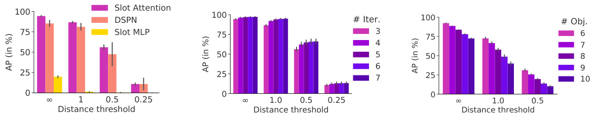
Figure 5: (Left) AP at different distance thresholds on CLEVR10 (with $K=10$ ). (Center) AP for the Slot Attention model with different number of iterations. The models are trained with 3 iterations and tested with iterations ranging from 3 to 7. (Right) AP for Slot Attention trained on CLEVR6 $K=6$ ) and tested on scenes containing exactly $N$ objects (with $N=K$ from 6 to 10).

图 5: (左) CLEVR10数据集在不同距离阈值下的平均精度(AP) (K=10)。(中) Slot Attention模型在不同迭代次数下的AP表现。模型训练时使用3次迭代，测试时迭代次数从3到7不等。(右) 在CLEVR6数据集(K=6)上训练的Slot Attention模型，在包含恰好N个物体(N=K，从6到10)的场景中的测试AP表现。

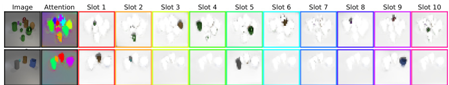
Figure 6: Visualization of the attention masks on CLEVR10 for two examples with 9 and 4 objects, respectively, for a model trained on the property prediction task. The masks are upsampled to $128\times128$ for this visualization to match the resolution of input image.

图 6: 在CLEVR10数据集上针对属性预测任务训练的模型，分别对包含9个和4个对象的两个示例进行注意力掩码可视化。为匹配输入图像分辨率，掩码被上采样至$128\times128$尺寸。

We visualize discovered object segmentation s in Figure 3 for all three datasets. The model learns to keep slots empty (only capturing the background) if there are more slots than objects. We find that Slot Attention typically spreads the uniform background across all slots instead of capturing it in just a single slot, which is likely an artifact of the attention mechanism that does not harm object disentanglement or reconstruction quality. We further visualize how the attention mechanism segments the scene over the individual attention iterations, and we inspect scene reconstructions from each individual iteration (the model has been trained to reconstruct only after the final iteration). It can be seen that the attention mechanism learns to specialize on the extraction of individual objects already at the second iteration, whereas the attention map of the first iteration still maps parts of multiple objects into a single slot.

我们在图3中展示了所有三个数据集上发现的目标分割结果。当槽位数量多于物体时，模型会学习保持部分槽位为空（仅捕捉背景）。我们发现Slot Attention通常会将均匀背景分散到所有槽位中，而非仅用单个槽位捕捉，这可能是注意力机制的特性，但并不影响物体解耦或重建质量。我们进一步可视化了注意力机制在每次迭代过程中如何分割场景，并检查了每次迭代后的场景重建结果（模型被设计为仅在最终迭代后执行重建）。可以看出，注意力机制在第二次迭代时已学会专注于提取单个物体，而第一次迭代的注意力图仍会将多个物体的部分区域映射到同一个槽位。

To evaluate whether Slot Attention can perform segmentation without relying on color cues, we further run experiments on a binarized version of multi-dSprites with white objects on black background, and on a greyscale version of CLEVR6. We use the binarized multi-dSprites dataset from Kabra et al. [83], for which Slot Attention achieves $69.4\pm0.9%$ ARI using $K=4$ slots, compared to $64.8\pm17.2%$ for IODINE [16] and $68.5\pm1.7%$ for R-NEM [39], as reported in [16]. Slot Attention performs competitively in decomposing scenes into objects based on shape cues only. We visualize discovered object segmentation s for the Slot Attention model trained on greyscale CLEVR6 in Figure 4, which Slot Attention handles without issue despite the lack of object color as a distinguishing feature.

为评估 Slot Attention 能否在不依赖颜色线索的情况下执行分割任务，我们进一步在二值化版本的多精灵数据集（白底黑物）和灰度版CLEVR6上进行了实验。我们采用Kabra等人[83]提供的二值化多精灵数据集，其中Slot Attention使用K=4个槽位获得$69.4\pm0.9%$的调整兰德指数(ARI)，而IODINE[16]和R-NEM[39]分别取得$64.8\pm17.2%$和$68.5\pm1.7%$的成绩（数据引自[16]）。Slot Attention在仅依靠形状线索分解场景物体时表现出竞争力。图4展示了在灰度CLEVR6上训练的Slot Attention模型发现的物体分割效果，该模型即使缺乏物体颜色作为区分特征仍能无误处理。

As our object discovery architecture uses the same decoder and reconstruction loss as IODINE [16], we expect it to similarly struggle with scenes containing more complicated backgrounds and textures. Utilizing different perceptual [49, 89] or contrastive losses [46] could help overcome this limitation. We discuss further limitations and future work in Section 5 and in the supplementary material.

由于我们的物体发现架构采用了与IODINE [16]相同的解码器和重建损失函数，预计在包含更复杂背景和纹理的场景中同样会遇到困难。采用不同的感知损失 [49, 89] 或对比损失 [46] 可能有助于克服这一局限。我们将在第5节和补充材料中进一步讨论相关局限性与未来工作方向。

Summary Slot Attention is highly competitive with prior approaches on unsupervised scene decomposition, both in terms of quality of object segmentation and in terms of training speed and memory efficiency. At test time, Slot Attention can be used without a decoder to obtain object-centric representations from an unseen scene.

摘要 Slot Attention 在无监督场景分解任务中与现有方法相比极具竞争力，无论是物体分割质量还是训练速度与内存效率方面。在测试阶段，Slot Attention 无需解码器即可从未见过的场景中获取以物体为中心的表示。

4.2 Set Prediction

4.2 集合预测

Training We train our model using the same hyper parameters as in Section 4.1 except we use a batch size of 512 and striding in the encoder. On CLEVR10, we use $K=10$ object slots to be in line with [31]. The Slot Attention model is trained using a single NVIDIA Tesla V100 GPU with 16GB of RAM.

训练
我们使用与第4.1节相同的超参数训练模型，但将批量大小设为512并在编码器中采用跨步处理。在CLEVR10数据集上，我们设置$K=10$个对象槽位以与[31]保持一致。Slot Attention模型使用单块16GB显存的NVIDIA Tesla V100 GPU进行训练。

Metrics Following Zhang et al. [31], we compute the Average Precision (AP) as commonly used in object detection [90]. A prediction (object properties and position) is considered correct if there is a matching object with exactly the same properties (shape, material, color, and size) within a certain distance threshold ( $\infty$ means we do not enforce any threshold). The predicted position coordinates are scaled to $[-3,3]$ . We zero-pad the targets and predict an additional indicator score in $[0,1]$ corresponding to the presence probability of an object (1 means there is an object) which we then use as prediction confidence to compute the AP.

指标
遵循 Zhang 等人 [31] 的方法，我们采用目标检测 [90] 中常用的平均精度 (Average Precision, AP) 作为评估指标。若预测结果（物体属性与位置）在特定距离阈值内（$\infty$ 表示不设阈值）存在属性完全匹配（形状、材质、颜色和尺寸）的物体，则判定为正确预测。预测位置坐标被归一化至 $[-3,3]$ 区间。我们对目标进行零填充，并额外预测一个 $[0,1]$ 区间的指示分数表示物体存在概率（1代表存在物体），该分数将作为预测置信度用于计算 AP。

Results In Figure 5 (left) we report results in terms of Average Precision for supervised object property prediction on CLEVR10 (using $T=3$ for Slot Attention at both train and test time). We compare to both the DSPN results of [31] and the Slot MLP baseline. Overall, we observe that our approach matches or outperforms the DSPN baseline. The performance of our method degrades gracefully at more challenging distance thresholds (for the object position feature) maintaining a reasonably small variance. Note that the DSPN baseline [31] uses a significantly deeper ResNet 34 [22] image encoder. In Figure 5 (center) we observe that increasing the number of attention iterations at test time generally improves performance. Slot Attention can naturally handle more objects at test time by changing the number of slots. In Figure 5 (right) we observe that the AP degrades gracefully if we train a model on CLEVR6 (with $K=6$ slots) and test it with more objects.

结果
在图5（左）中，我们报告了CLEVR10监督式物体属性预测的平均精度（Average Precision）结果（训练和测试时均使用$T=3$的Slot Attention）。我们将其与[31]的DSPN结果以及Slot MLP基线进行比较。总体而言，我们的方法达到或超越了DSPN基线的性能。在更具挑战性的距离阈值（针对物体位置特征）下，我们的方法性能下降平缓，并保持了较小的方差。需要注意的是，DSPN基线[31]使用了更深的ResNet 34 [22]图像编码器。

在图5（中）中，我们观察到在测试时增加注意力迭代次数通常会提升性能。Slot Attention通过改变slot数量，可以自然地处理测试时更多的物体。

在图5（右）中，我们观察到：如果在CLEVR6（使用$K=6$个slot）上训练模型，并用更多物体进行测试时，平均精度（AP）会平缓下降。

Intuitively, to solve this set prediction task each slot should attend to a different object. In Figure 6, we visualize the attention maps of each slot for two CLEVR images. In general, we observe that the attention maps naturally segment the objects. We remark that the method is only trained to predict the property of the objects, without any segmentation mask. Quantitatively, we can evaluate the Adjusted Rand Index (ARI) scores of the attention masks. On CLEVR10 (with masks), the attention masks produced by Slot Attention achieve an ARI of $78.0%\pm2.9$ (to compute the ARI we downscale the input image to $32\times32$ ). Note that the masks evaluated in Table 1 are not the attention maps but are predicted by the object discovery decoder.

直观上，为完成这一集合预测任务，每个槽(slot)应关注不同对象。在图6中，我们可视化了两张CLEVR图像中各槽的注意力图。总体而言，我们观察到注意力图能自然分割出物体。需要强调的是，该方法仅通过预测物体属性进行训练，未使用任何分割掩码。量化评估方面，我们计算了注意力掩码的调整兰德指数(ARI)得分。在CLEVR10(带掩码版本)上，Slot Attention生成的注意力掩码ARI达到$78.0%\pm2.9$(计算ARI时将输入图像降采样至$32\times32$)。需注意表1中评估的掩码并非注意力图，而是由物体发现解码器预测所得。

Summary Slot Attention learns a representation of objects for set-structured property prediction tasks and achieves results competitive with a prior state-of-the-art approach while being significantly easier to implement and tune. Further, the attention masks naturally segment the scene, which can be valuable for debugging and interpreting the predictions of the model.

摘要 Slot Attention 通过学习集合结构属性预测任务中的对象表示，取得了与先前最先进方法相媲美的结果，同时实现和调参难度显著降低。此外，注意力掩码能自然分割场景，这对调试和解释模型预测具有重要价值。

5 Conclusion

5 结论

We have presented the Slot Attention module, a versatile architectural component that learns objectcentric abstract representations from low-level perceptual input. The iterative attention mechanism used in Slot Attention allows our model to learn a grouping strategy to decompose input features into a set of slot representations. In experiments on unsupervised visual scene decomposition and supervised object property prediction we have shown that Slot Attention is highly competitive with prior related approaches, while being more efficient in terms of memory consumption and computation.

我们提出了Slot Attention模块，这是一种多功能架构组件，能够从低层次感知输入中学习以物体为中心的抽象表征。Slot Attention采用的迭代注意力机制使模型能够学习分组策略，将输入特征分解为一组槽位(slot)表征。在无监督视觉场景分解和有监督物体属性预测实验中，我们证明了Slot Attention与现有相关方法相比具有高度竞争力，同时在内存消耗和计算效率方面更为高效。

A natural next step is to apply Slot Attention to video data or to other data modalities, e.g. for clustering of nodes in graphs, on top of a point cloud processing backbone or for textual or speech data. It is also promising to investigate other downstream tasks, such as reward prediction, visual reasoning, control, or planning.

自然延伸的方向是将Slot Attention应用于视频数据或其他模态数据，例如在图数据上基于点云处理主干进行节点聚类，或用于文本和语音数据。探索其他下游任务也颇具前景，例如奖励预测、视觉推理、控制或规划。

Broader Impact

更广泛的影响

The Slot Attention module allows to learn object-centric representations from perceptual input. As such, it is a general module that can be used in a wide range of domains and applications. In our paper, we only consider artificially generated datasets under well-controlled settings where slots are expected to specialize to objects. However, the specialization of our model is implicit and fully driven by the downstream task. We remark that as a concrete measure to assess whether the module specialized in unwanted ways, one can visualize the attention masks to understand how the input features are distributed across the slots (see Figure 6). While more work is required to properly address the usefulness of the attention coefficients in explaining the overall predictions of the network (especially if the input features are not human interpret able), we argue that they may serve as a step towards more transparent and interpret able predictions.

槽注意力（Slot Attention）模块能够从感知输入中学习以物体为中心的表示。因此，它是一个通用模块，可广泛应用于多个领域和场景。在本文中，我们仅考虑受控环境下人工生成的数据集，其中槽（slot）预期会专门对应物体。然而，我们模型的 specialization 是隐式的，完全由下游任务驱动。需要指出的是，作为评估该模块是否以非预期方式实现 specialization 的具体方法，可通过可视化注意力掩码来理解输入特征在槽间的分布情况（见图 6）。虽然要准确评估注意力系数在解释网络整体预测时的有效性仍需更多工作（尤其是当输入特征不具备人类可解释性时），我们认为这可能是迈向更透明、可解释预测的一步。

Acknowledgements

致谢

We would like to thank Nal Kal ch brenner for general advise and feedback on the paper, Mostafa Dehghani, Klaus Greff, Bernhard Schölkopf, Klaus-Robert Müller, Adam Kosiorek, and Peter Battaglia for helpful discussions, and Rishabh Kabra for advise regarding the DeepMind Multi-Object Datasets.

我们要感谢Nal Kalchbrenner对论文的总体建议和反馈，Mostafa Dehghani、Klaus Greff、Bernhard Schölkopf、Klaus-Robert Müller、Adam Kosiorek和Peter Battaglia的有益讨论，以及Rishabh Kabra关于DeepMind多对象数据集的建议。

References

参考文献

Supplementary Material for Object-Centric Learning with Slot Attention

基于Slot Attention的物体中心学习补充材料

In Section A, we highlight some limitations of our work as well as potential directions for future work. In Section B, we report results of an ablation study on Slot Attention. In Section C, we report further qualitative and quantitative results. In Section D, we give the proof for Proposition 1. In Section E, we report details on our implementation and experimental setting.

在A部分，我们重点介绍了本研究的局限性以及未来工作的潜在方向。B部分报告了Slot Attention的消融实验结果。C部分展示了更多定性和定量分析结果。D部分给出了命题1的证明过程。E部分详细说明了实现方法和实验设置。

A Limitations

A 局限性

We highlight several limitations of the Slot Attention module that could potentially be addressed in future work:

我们指出了Slot Attention模块的几个局限性，这些局限性可能在未来的工作中得到解决：

Background treatment The background of a scene receives no special treatment in Slot Attention as all slots use the same representational format. Providing special treatment for backgrounds (e.g., by assigning a separate background slot) is interesting for future work.

背景处理
在Slot Attention中，场景背景未作特殊处理，因为所有槽(slot)都使用相同的表示格式。为背景提供特殊处理（例如分配单独的背景槽）是未来工作中值得探索的方向。

Translation symmetry The positional encoding used in our experiments is absolute and hence our module is not e qui variant to translations. Using a patch-based object extraction process as in [44] or an attention mechanism with relative positional encoding [91] are promising extensions.

平移对称性
我们实验中使用的位置编码是绝对式的，因此我们的模块不具备平移等变性。采用基于图像块的对象提取方法 [44] 或结合相对位置编码的注意力机制 [91] 是值得探索的扩展方向。

Type of clustering Slot Attention does not know about objects per-se: segmentation is solely driven by the downstream task, i.e., Slot Attention does not distinguish between clustering objects, colors, or simply spatial regions, but relies on the downstream task to drive the specialization to objects.

聚类类型
Slot Attention 本身并不了解物体：分割完全由下游任务驱动，即 Slot Attention 不会区分聚类物体、颜色或仅仅是空间区域，而是依赖下游任务来驱动对物体的专门化处理。

Communication between slots In Slot Attention, slots only communicate via the softmax attention over the input keys, which is normalized across slots. This choice of normalization establishes competition between the slots for explaining parts of the input, which can drive specialization of slots to objects. In some scenarios it can make sense to introduce a more explicit form of communication between slots, e.g. via slot-to-slot message passing in the form of a graph neural network as in [9, 46] or self-attention [20, 53, 60, 63, 67]. This can be beneficial for modeling systems of objects that interact dynamically [9, 46, 67] or for set generation conditioned on a single vector (as opposed to an image or a set of vectors) [60].

槽之间的通信
在Slot Attention中，槽仅通过输入键的softmax注意力进行通信，该注意力在槽之间归一化。这种归一化方式促使槽之间为解释输入部分展开竞争，从而驱动槽针对对象实现专业化。在某些场景下，引入更显式的槽间通信形式可能更为合理，例如通过图神经网络形式的槽间消息传递[9,46]或自注意力机制[20,53,60,63,67]。这对于建模动态交互的对象系统[9,46,67]或基于单个向量（而非图像或向量集合）的条件集合生成任务[60]具有优势。

B Model Ablations

B 模型消融实验

In this section, we investigate the importance of individual components and modeling choices in the Slot Attention module and compare our default choice to a variety of reasonable alternatives. For simplicity, we report all results on a smaller validation set consisting of 500 validation images for property prediction (instead of 15K) and on 320 training images for object discovery. In the unsupervised case, results on the training set and on held-out validation examples are nearly identical.

在本节中，我们研究了Slot Attention模块中各个组件和建模选择的重要性，并将我们的默认选择与多种合理替代方案进行了比较。为简化起见，所有结果均在由500张验证图像组成的较小验证集（而非15K）上报告属性预测性能，并在320张训练图像上报告物体发现性能。在无监督情况下，训练集和保留验证集的结果几乎相同。

Value aggregation In Figure 7, we show the effect of taking a weighted sum as opposed to a weighted average in Line 8 of Algorithm 1. The average stabilizes training and yields significantly higher ARI and Average Precision scores (especially at the more strict distance thresholds). We can obtain a similar effect by replacing the weighted mean with a weighted sum followed by layer normalization (LayerNorm) [23].

价值聚合
在图7中，我们展示了算法1第8行采用加权求和与加权平均的效果差异。加权平均能稳定训练过程，并显著提升ARI和平均精确度 (Average Precision) 得分（尤其在更严格的距离阈值下）。若将加权平均替换为加权求和后接层归一化 (LayerNorm) [23]，也可获得类似效果。

Position embedding In Figure 8, we observe that the position embedding is not necessary for predicting categorical object properties. However, the performance in predicting the object position clearly decreases if we remove the position embedding. Similarly, the ARI score in unsupervised object discovery is significantly lower when not adding positional information to the CNN feature maps before the Slot Attention module.

位置嵌入
在图 8 中，我们观察到位置嵌入对于预测分类物体属性并非必要。然而，如果移除位置嵌入，物体位置预测的性能会明显下降。类似地，如果在 Slot Attention 模块之前未向 CNN 特征图添加位置信息，无监督物体发现中的 ARI 分数会显著降低。

Slot initialization In Figure 9, we show the effect of learning a separate set of Gaussian mean and variance parameters for the initialization of each slot compared to the default setting of using a shared set of parameters for all slots. We observe that a per-slot parameter iz ation can increase performance slightly for the supervised task, but decreases performance on the unsupervised task, compared to the default shared parameter iz ation. We remark that when learning a separate set of parameters for each slot, adding additional slots at test time is not possible without re-training.

槽位初始化
在图 9 中，我们展示了为每个槽位的初始化学习单独的高斯均值与方差参数的效果，并与默认所有槽位共享同一组参数的设置进行对比。实验表明，相比默认的共享参数方式，为每个槽位单独学习参数能在监督任务中略微提升性能，但在无监督任务中会降低性能。需要注意的是，若为每个槽位学习独立参数，则测试时无法在不重新训练的情况下新增槽位。

Attention normalization axis In Figure 10, we highlight the role of the softmax axis in the attention mechanism, i.e., over which dimension the normalization is performed. Taking the softmax over the slot axis induces competition among the slots for explaining parts of the input. When we take the softmax over the input axis instead (as done in regular self-attention), the attention coefficients for each slot will be independent of all other slots, and hence slots have no means of exchanging information, which significantly harms performance on both tasks.

注意力归一化轴
在图 10 中，我们强调了 softmax 轴在注意力机制中的作用，即归一化操作所沿的维度。在 slot 轴上进行 softmax 会促使各 slot 之间为解释输入部分而竞争。若改为在输入轴上执行 softmax (如常规自注意力机制的做法)，每个 slot 的注意力系数将独立于其他 slot，导致 slot 间无法交换信息，这会显著损害两项任务的性能。

Recurrent update function In Figure 11, we highlight the role of the GRU in learning the update function for the slots as opposed to simply taking the output of Line 8 as the next value for the slots. We observe that the learned update function yields a noticable improvement.

循环更新函数
在图 11 中，我们强调了 GRU 在学习槽位更新函数中的作用，而不是简单地将第 8 行的输出作为槽位的下一个值。我们观察到学习到的更新函数带来了显著改进。

Attention iterations In Figure 12, we show the impact of the number of attention iterations while training. We observe a clear benefit in having more than a single attention iteration. Having more than 3 attention iterations significantly slows down training convergence, which results in lower performance when trained for the same number of steps. This can likely be mitigated by instead decoding and applying a loss at every attention iteration as opposed to only the last one. We note that at test time, using more than 3 attention iterations (even when trained with only 3 iterations) generally improves performance.

注意力迭代次数
在图 12 中，我们展示了训练过程中注意力迭代次数的影响。观察到使用超过单次注意力迭代能带来明显收益。超过3次注意力迭代会显著减缓训练收敛速度，导致相同训练步数下性能下降。这一问题可能通过每次注意力迭代都进行解码并计算损失（而非仅在最后一次）来缓解。值得注意的是，在测试阶段，使用超过3次注意力迭代（即使训练时仅用3次）通常能提升性能。

Layer normalization In Figure 13, we show that applying layer normalization (LayerNorm) [23] to the inputs and to the slot representations at each iteration in the Slot Attention module improves predictive performance. For set prediction, it particularly improves its ability to predict position accurately, likely because it leads to faster convergence at training time.

层归一化
在图 13 中，我们展示了在 Slot Attention 模块的每次迭代中对输入和槽表示应用层归一化 (LayerNorm) [23] 可以提升预测性能。对于集合预测任务，该方法尤其能提高位置预测的准确性，这可能是因为它在训练时能加快收敛速度。

Feed forward network In Figure 14, we show that the residual MLP after the GRU is optional and may slow down convergence in property prediction, but may slightly improve performance on object discovery.

前馈网络
在图 14 中，我们展示了 GRU 之后的残差 MLP (多层感知机) 是可选的，它可能会减缓属性预测的收敛速度，但可能略微提升物体发现任务的性能。

Softmax temperature In Figure 15, we show the effect of the softmax temperature. The scaling of $\sqrt{D}$ clearly improves the performance on both tasks.

softmax温度
在图15中，我们展示了softmax温度的影响。$\sqrt{D}$的缩放明显提升了两个任务的性能。

Offset for numerical stability In Figure 16, we show that adding a small offset to the attention maps (for numerical stability) as in Algorithm 1 compared to the alternative of adding an offset to the denominator in the weighted mean does not significantly change the result in either task.

数值稳定性的偏移量

在图 16 中，我们展示了在注意力图中添加一个小偏移量（用于数值稳定性），如算法 1 所示，与在加权平均的分母中添加偏移量的替代方案相比，这两种方法在两项任务中均未显著改变结果。

Learning rate schedules In Figure 17 and 18, we show the effect of our decay and warmup schedules. While we observe a clear benefit from the decay schedule, the warmup seem to be mostly useful in the object discovery setting, where it helps avoid failure cases of getting stuck in a suboptimal solution (e.g., clustering the image into stripes as opposed to objects).

学习率调度
在图 17 和图 18 中，我们展示了衰减 (decay) 和预热 (warmup) 调度策略的效果。虽然衰减策略带来了明显的收益，但预热策略似乎主要在物体发现 (object discovery) 场景中发挥作用，它有助于避免陷入次优解（例如将图像聚类为条纹而非物体）的失败情况。

Number of training slots In Figure 19, we show the effect of training with a larger number of slots than necessary. We train both the object discovery and property prediction methods on CLEVR6 with the number of slots we used in our CLEVR10 experiments (note that for object discovery we use an additional slot to be consistent with the baselines). We observe that knowing the precise number of objects in the dataset is generally not required. Training with more slots may even help in the property prediction experiments and is slightly harmful in the object discovery. Overall, this indicates that the model is rather robust to the number of slots (given enough slots to model each object independently). Using a (rough) upper bound to the number of objects in the dataset seem to be a reasonable selection strategy for the number of slots.

训练槽数量
在图19中，我们展示了使用多于必要数量的训练槽进行训练的效果。我们在CLEVR6数据集上使用CLEVR10实验中的槽数量（注意对于物体发现任务，为与基线保持一致我们额外增加了一个槽），同时训练物体发现和属性预测方法。实验表明，通常无需精确知道数据集中的物体数量。使用更多槽训练甚至有助于属性预测实验，而对物体发现任务仅有轻微负面影响。总体而言，这表明模型对槽数量具有较强鲁棒性（只要提供足够槽位使每个物体能被独立建模）。采用数据集中物体数量的（粗略）上限作为槽数量选择策略是合理的。

Soft k-means Slot Attention can be seen as a generalized version of the soft k-means algorithm [73]. We can reduce Slot Attention to a version of soft $\mathbf{k}$ -means with a dot-product scoring function (as opposed to the negative Euclidean distance) by simultaneously replacing the GRU update, all LayerNorm functions and the key/query/value projections with the identity function. Specifically, instead of the GRU update, we simply take the output of Line 8 in Algorithm 1 as the next value for the slots. With these ablations, the model achieves $75.5\pm3.8%$ ARI on CLEVR6, compared to $98.8\pm0.3%$ for the full version of Slot Attention.

软k均值 (soft k-means) 的Slot Attention可视为软k均值算法[73]的广义版本。通过同时用恒等函数替换GRU更新、所有LayerNorm函数及键/查询/值投影操作，我们可以将Slot Attention简化为采用点积评分函数（而非负欧氏距离）的软k均值变体。具体而言，我们不使用GRU更新，而是直接取算法1第8行的输出作为槽(slot)的下一状态值。经过这些消融后，该模型在CLEVR6上达到$75.5\pm3.8%$的ARI值，而完整版Slot Attention的表现为$98.8\pm0.3%$。

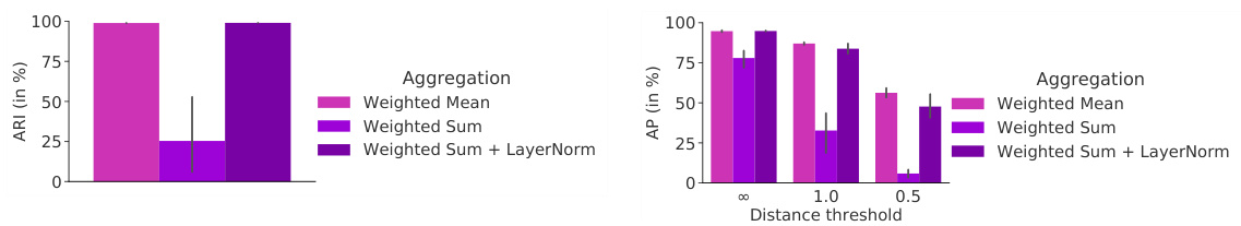
Figure 7: Aggregation function variants (Line 8) for object discovery on CLEVR6 (left) and property prediction on CLEVR10 (right).

图 7: CLEVR6数据集上的物体发现任务(左)和CLEVR10数据集上的属性预测任务(右)中使用的聚合函数变体(第8行)。

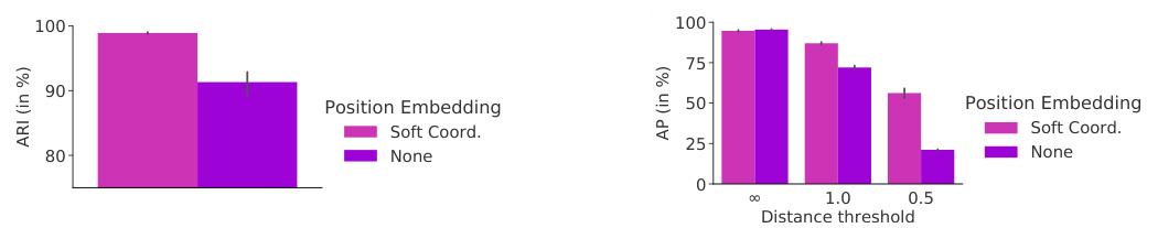
Figure 8: Ablation on the position embedding for object discovery on CLEVR6 (left) and property prediction on CLEVR10 (right).

图 8: CLEVR6(左)物体发现和CLEVR10(右)属性预测中位置嵌入的消融实验。

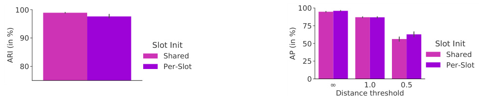
Figure 9: Slot initialization variants for object discovery on CLEVR6 (left) and property prediction on CLEVR10 (right).

图 9: CLEVR6 (左) 物体发现的槽初始化变体及 CLEVR10 (右) 属性预测的槽初始化变体。

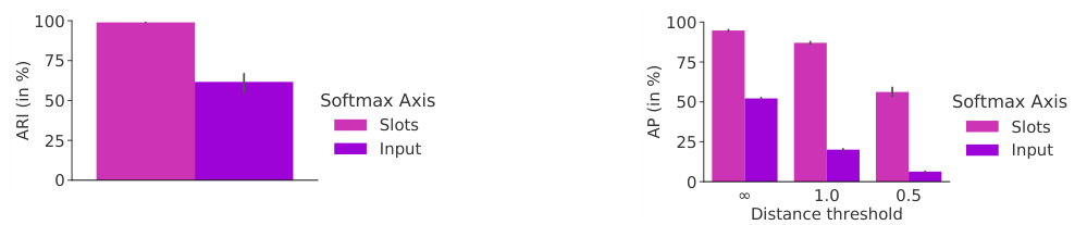
Figure 10: Choice of softmax axis for object discovery on CLEVR6 (left) and property prediction on CLEVR10 (right).

图 10: CLEVR6数据集上物体发现的softmax轴选择(左)与CLEVR10数据集上属性预测的softmax轴选择(右)。

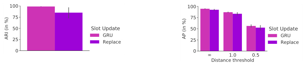
Figure 11: Slot update function variants for object discovery on CLEVR6 (left) and property prediction on CLEVR10 (right).

图 11: CLEVR6 (左) 物体发现任务和 CLEVR10 (右) 属性预测任务的槽位更新函数变体对比。

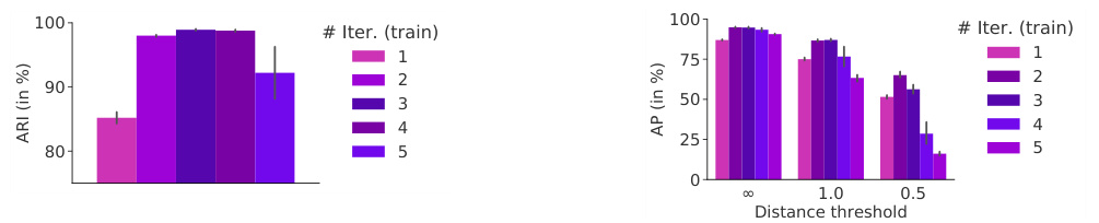
Figure 12: Number of attention iterations during training for object discovery on CLEVR6 (left) and property prediction on CLEVR10 (right).

图 12: CLEVR6 (左)物体发现和CLEVR10 (右)属性预测训练过程中的注意力迭代次数。

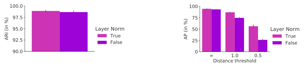
Figure 13: LayerNorm in the Slot Attention Module for object discovery on CLEVR6 (left) and property prediction on CLEVR10 (right).

图 13: Slot Attention模块中的LayerNorm在CLEVR6上的物体发现(左)和CLEVR10上的属性预测(右)效果。

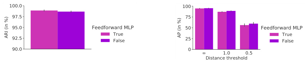
Figure 14: Optional feed forward MLP for object discovery on CLEVR6 (left) and property prediction on CLEVR10 (right).

图 14: 用于 CLEVR6 物体发现 (左) 和 CLEVR10 属性预测 (右) 的可选前馈 MLP (Multilayer Perceptron)。

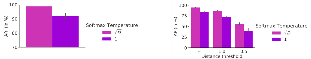
Figure 15: Softmax temperature in the Slot Attention Module for object discovery on CLEVR6 (left) and property prediction on CLEVR10 (right).

图 15: CLEVR6物体发现任务(左)和CLEVR10属性预测任务(右)中Slot Attention模块的Softmax温度参数。

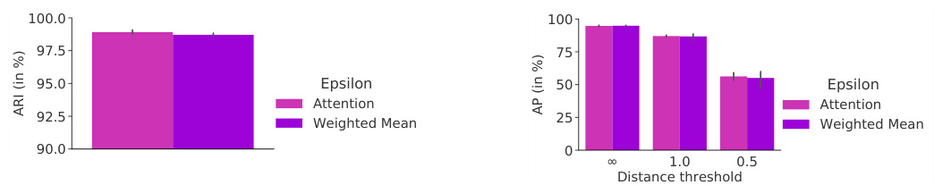
Figure 16: Offset in the attention maps or the denominator of the weighted mean for object discovery on CLEVR6 (left) and property prediction on CLEVR10 (right).

图 16: CLEVR6 (左) 物体发现任务和 CLEVR10 (右) 属性预测任务中注意力图或加权平均分母的偏移量。

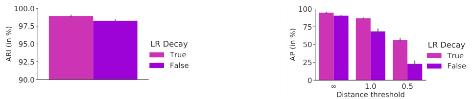
Figure 17: Learning rate decay for object discovery on CLEVR6 (left) and property prediction on CLEVR10 (right).

图 17: CLEVR6 物体发现任务 (左) 和 CLEVR10 属性预测任务 (右) 的学习率衰减曲线。

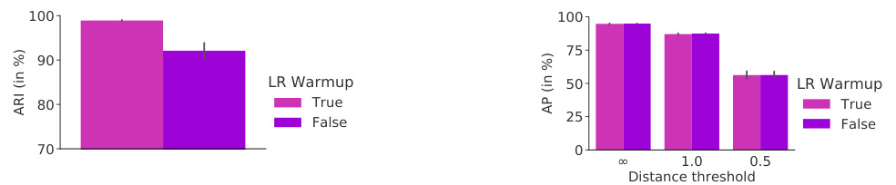
Figure 18: Learning rate warmup for object discovery on CLEVR6 (left) and property prediction on CLEVR10 (right).

图 18: CLEVR6 上的物体发现 (左) 和 CLEVR10 上的属性预测 (右) 的学习率预热曲线。

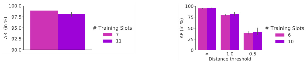
Figure 19: Number of training slots on CLEVR6 for object discovery (left) and property prediction (right).

图 19: CLEVR6数据集上用于物体发现(左)和属性预测(右)的训练槽位数量。

C Further Experimental Results

C 更多实验结果

C.1 Object Discovery

C.1 目标发现

Runtime Experiments on a single V100 GPU with 16GB of RAM with $500\mathrm{k}$ steps and a batch size of 64 ran for approximately 7.5hrs for Tetrominoes, 24hrs for multi-dSprites, and 5 days, 13hrs for CLEVR6 (wall-clock time).

在一台配备16GB内存的V100 GPU上进行的运行时实验显示：以64的批次大小运行50万步时，Tetrominoes耗时约7.5小时，multi-dSprites耗时24小时，CLEVR6耗时5天13小时（实际挂钟时间）。

Qualitative results In Figure 20, we show qualitative segmentation results for a Slot Attention model trained on the object discovery task. This model is trained on CLEVR6 but uses $K=11$ instead of the default setting of $K=7$ slots during both training and testing, while all other settings remain unchanged. In this particular experiment, we trained 5 models using this setting with 5 different random seeds for model parameter initialization. Out of these 5 models, we found that a single model learned the solution of placing the background into a separate slot (which is the one we visualize). The typical solution that a Slot Attention-based model finds (for most random seeds) is to distribute the background equally over all slots, which is the solution we highlight in the main paper. In Figure 20 (bottom two rows), we further show how the model generalizes to scenes with more objects (up to 10) despite being trained on CLEVR6, i.e., on scenes containing a maximum of 6 objects.

定性结果
在图 20 中，我们展示了在物体发现任务上训练的 Slot Attention 模型的定性分割结果。该模型在 CLEVR6 上训练，但在训练和测试期间使用 $K=11$ 而非默认的 $K=7$ 个 slot，其余设置保持不变。在本实验中，我们使用该设置训练了 5 个模型，并采用 5 个不同的随机种子初始化模型参数。在这 5 个模型中，我们发现有一个模型学会了将背景分配到独立 slot 的解决方案（即我们可视化展示的模型）。基于 Slot Attention 的模型在大多数随机种子下找到的典型解决方案是将背景均匀分布到所有 slot 中，这也是我们在主论文中强调的解决方案。在图 20（底部两行）中，我们进一步展示了该模型如何泛化到包含更多物体（最多 10 个）的场景，尽管其训练数据 CLEVR6 最多仅包含 6 个物体。

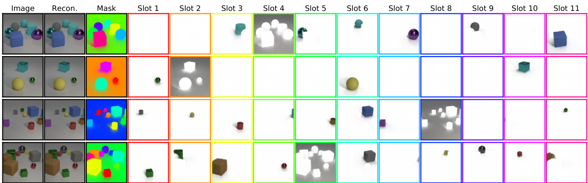
Figure 20: Visualization of overall reconstructions, alpha masks, and per-slot reconstructions for a Slot Attention model trained on CLEVR6 (i.e., on scenes with a maximum number of 6 objects), but tested on scenes with up to 10 objects, using $K=11$ slots both at training and at test time, and $T=3$ iterations at training time and $T=5$ iterations at test time. We only visualize examples where the objects were successfully clustered after $T=5$ iterations. For some random slot initialization s, clustering results still improve when run for more iterations. We note that this particular model learned to separate the background out into a separate (but random) slot instead of spreading it out evenly over all slots.

图 20: 在CLEVR6数据集(即最多包含6个物体的场景)上训练的Slot Attention模型,在测试时使用最多10个物体场景的整体重建效果、alpha遮罩及逐槽位重建可视化。训练和测试均采用$K=11$个槽位,训练时迭代次数$T=3$,测试时$T=5$。仅展示经过$T=5$次迭代后成功聚类物体的案例。某些随机初始化的槽位经过更多迭代后聚类效果仍会提升。值得注意的是,该特定模型学会了将背景分离至单独(但随机)的槽位,而非均匀分散至所有槽位。

C.2 Set Prediction

C.2 集合预测

Runtime Experiments on a single V100 GPU with 16GB of RAM with 150k steps and a batch size of 512 ran for approximately 2 days and 3hrs for CLEVR (wall-clock time).

在配备16GB内存的单个V100 GPU上运行实验，使用15万步训练步长和512的批量大小，CLEVR任务耗时约2天3小时（实际挂钟时间）。

Qualitative results In Table 2, we show the predictions and attention coefficients of a Slot Attention model on several challenging test examples for the supervised property prediction task. The model was trained with default settings $T=3$ attention iterations) and the images are selected by hand to highlight especially difficult cases (e.g., multiple identical objects or many partially overlapping objects in one scene). Overall, we can see that the property prediction typically becomes more accurate with more iterations, although the accuracy of the position prediction may decrease. This is not surprising as we only apply the loss at $t=3$ , and generalization to more time steps at test time is not guaranteed. We note that one could alternatively apply the loss at every iteration during training, which has the potential to improve accuracy, but would increase computational cost. We observe that the model appears to handle multiple copies of the same object well (top). On very crowded scenes (middle and bottom), we note that the slots have a harder time segmenting the scene, which can lead to errors in the prediction. However, more iterations seem to sharpen the segmentation which in turns improves predictions.

定性结果
在表2中，我们展示了Slot Attention模型在有监督属性预测任务中若干挑战性测试样本的预测结果和注意力系数。该模型采用默认设置训练（$T=3$次注意力迭代），并手动选取图像以突出特别困难的案例（例如场景中存在多个相同物体或大量部分重叠物体）。总体而言，我们可以看到随着迭代次数增加，属性预测通常会变得更准确，尽管位置预测的精度可能下降。这并不意外，因为我们仅在$t=3$时应用损失函数，且无法保证测试时向更多时间步长的泛化能力。我们注意到，另一种方法是在训练期间每次迭代都应用损失函数，这有可能提高精度，但会增加计算成本。观察发现，该模型似乎能较好地处理同一物体的多个副本（顶部）。在非常拥挤的场景中（中部和底部），我们发现槽（slots）更难分割场景，这可能导致预测错误。不过，更多迭代似乎能锐化分割效果，从而改进预测。

Table 2: Example predictions of a Slot Attention model trained with $T=3$ on a challenging example with 4 objects (two of which are identical and partially overlapping) and crowded scenes with 10 objects. We highlight wrong prediction of attributes and distances greater than 0.5.

		Image	Attn.t=1	Attn.t=2	Attn.t=3	Attn.t=4	Attn.t=5
True Y Pred. t=1				Pred. t=2				Pred. t=4
(-2.11, -0.69, 0.70)
(2.41, -0.82, 0.70) large yellow metal cube		(-2.82,-0.19, 0.71), d=0.87	(-2.43, -0.22, 0.70), d=0.56 large blue rubber cylinder			Pred. t=3 (-2.42, -0.55, 0.71), d=0.34 large blue rubber cylinder			Pred. t=5 (-2.42, -0.48, 0.71), d=0.36
		large blue rubber cylinder large blue rubber cylinder				(2.53, -0.83, 0.71), d=0.12		(-2.41, -0.35, 0.71), d=0.45 large blue rubber cylinder		large blue rubber cylinder
		(2.52, -0.35, 0.66), d=0.48 large yellow metal cube		(2.57, -0.64, 0.72), d=0.24 large yellow metal cube (-2.70, 2.31, 0.34), d=0.45		large yellow metal cube (-2.57,2.35, 0.33), d=0.47		(2.55, -0.79, 0.70), d=0.14 large yellow metal cube (-2.58, 2.35, 0.34), d=0.48		(2.54, -0.82, 0.71), d=0.13 large yellow metal cube (-2.58, 2.35, 0.34), d=0.48
		(-2.57, 1.88, 0.35) (-2.19,2.23, 0.37),d=0.52
		small purple rubber cylinder (0.69, -1.51, 0.70)	small purple rubber cylinder small purple rubber cylinder (0.26, -2.05,0.67),d=0.69 (0.72, -1.47, 0.70), d=0.05						small purple rubber cylinder small purple rubber cylinder (0.71, -1.54, 0.69), d=0.03 (0.72, -1.55, 0.69), d=0.04
		large blue rubber cylinder	large blue rubber cylinder large blue rubber cylinder						large blue rubber cylinder large blue rubber cylinder
							Attn. t=4
			Image	Attn.t=1	Attn.t=2	Attn.t=3		Attn.t=5
True Y Pred. t=1 (-2.92, 0.03, 0.70)
					Pred. t=3					Pred. t=5
large green metal cylinder	(-2.36, -1.24, 0.68), d=1.39 (-0.90, 0.35, 0.57), d=2.05				(-2.24,0.16, 0.71), d=0.70				Pred. t=4
(-1.41, 2.57, 0.35)	large greenmetal cylinder				large greenmetal cylinder				(-2.38,-0.04,0.68),d=0.55	(-2.36, 0.03, 0.69), d=0.56
	(-0.47, 2.41, 0.40), d=0.95	large green metal cylinder						(-1.98, 2.10,0.36), d=0.74		large greenmetal cylinder
		(-1.58, 2.11, 0.25), d=0.50			(-1.65,1.99,0.34),d=0.63			large greenmetal cylinder		(-1.92, 2.24, 0.36), d=0.61
small gray metal cylinder	small graymetal cylinder	small gray metal cylinder			small gray metal cylinder			small gray metal cylinder
(0.33, 2.72, 0.35)	(0.28,1.34,0.38),d=1.38			(0.27, 1.06, 0.33), d=1.66			(-1.44, 1.56, 0.35), d=2.11		(-0.56, 1.16, 0.23), d=1.80	small gray metal cylinder (-0.71, 1.24, 0.34), d=1.81
small blue metal sphere	small blue metal sphere			small blue metal sphere			smali blue metal sphere	small blue metal sphere		small blue metal sphere
(2.22, -2.28, 0.35)	(2.05, -1.94, 0.37), d=0.38			(2.28,-2.02,0.37),d=0.27			(2.10,-2.03, 0.36), d=0.28	(2.10, -2.01, 0.36),d=0.30		(2.09,-2.01, 0.36), d=0.30
small red rubber cube	small red rubber cube			small red rubber cube			small red rubber cube	small red rubber cube		small red rubber cube
(1.99, -0.93, 0.70)	(2.03,-0.31, 0.68), d=0.62			(1.54, -1.04, 0.72), d=0.47			(1.90, -0.95, 0.72), d=0.09	(1.83, -0.90, 0.72),d=0.17		(1.86, -0.91, 0.72), d=0.14
large blue rubber cube	large blue rubber cube			large blue rubber cube			large blue rubber cube	large blue rubber cube		large blue rubber cube
(-1.50,-0.34, 0.35)	(-2.50, 0.14, 0.40), d=1.11			(-2.06,1.66,0.28), d=2.08	small blue metal sphere		(-0.11,0.72,0.33),d=1.76	small blue metal sphere	(-0.60, 1.13, 0.35), d=1.72	(-0.55,1.04, 0.32), d=1.68
small blue metal sphere	small gray metal cylinder (-1.54,0.85, 0.41), d=3.86			small gray metal cylinder (1.15, 2.35, 0.31), d=0.81	(1.85, 2.38, 0.37), d=0.16			(1.76, 2.38, 0.38), d=0.23		small blue metal sphere (1.81, 2.34, 0.37), d=0.22
(1.94, 2.51, 0.35)	large gray metal eylinder			small green metal sphere	small green metal sphere			small green metal sphere		small green metal sphere
small green metal sphere (-2.05, -2.99, 0.70)	(-0.45,-1.37,0.43),d=2.30			(-2.53, -2.33,0.69), d=0.82			(-1.53,-2.54, 0.72), d=0.69	(-2.30, -2.61, 0.71), d=0.45		(-2.09, -2.51, 0.70), d=0.48
large gray metal cylinder	large blue rubber cylinder			large graymetal cylinder	large gray rubber cylinder			large graymetal cylinder (-0.26, -2.69, 0.69), d=0.26		large graymetal cylinder
(-0.31,-2.95, 0.70)	(0.10, -2.59, 0.70), d=0.54			(-0.25,-2.50,0.70), d=0.45	(-0.26,-2.60, 0.69), d=0.35 large grayrubbercylinder			large grayrubber cylinder		(-0.29, -2.64, 0.69), d=0.31
large grayrubber cylinder (1.81,0.84,0.35)	large gray rubber cube (1.16, -1.06, 0.37), d=2.01			large gray rubber cylinder (0.27,0.66,-0.17), d=1.64			(1.49,0.32,0.33),d=0.62	(1.40,0.53,0.33).d=0.52		large gray rubber cylinder (1.40,0.50,0.33),d=0.54
small brown rubber sphere	large blue rubber cube			small brown rubber sphere			small brown rubber sphere	small brown rubber sphere		small brown rubber sphere

表 2: 使用 $T=3$ 训练的 Slot Attention 模型在包含 4 个物体（其中两个相同且部分重叠）的挑战性示例以及 10 个物体的拥挤场景中的预测示例。我们标出了属性预测错误和距离大于 0.5 的情况。

	图像	Attn.t=1	Attn.t=2	Attn.t=3	Attn.t=4	Attn.t=5
真实 Y 预测 t=1			预测 t=2					预测 t=4
								(-2.11, -0.69, 0.70)
(2.41, -0.82, 0.70) 大型黄色金属立方体	(-2.82,-0.19, 0.71), d=0.87		(-2.43, -0.22, 0.70), d=0.56 大型蓝色橡胶圆柱体		预测 t=3 (-2.42, -0.55, 0.71), d=0.34 大型蓝色橡胶圆柱体		预测 t=5 (-2.42, -0.48, 0.71), d=0.36
大型蓝色橡胶圆柱体大型蓝色橡胶圆柱体				(2.53, -0.83, 0.71), d=0.12		(-2.41, -0.35, 0.71), d=0.45 大型蓝色橡胶圆柱体	大型蓝色橡胶圆柱体
(2.52, -0.35, 0.66), d=0.48 大型黄色金属立方体		(2.57, -0.64, 0.72), d=0.24 大型黄色金属立方体 (-2.70, 2.31, 0.34), d=0.45			大型黄色金属立方体 (-2.57,2.35, 0.33), d=0.47		(2.55, -0.79, 0.70), d=0.14 大型黄色金属立方体 (-2.58, 2.35, 0.34), d=0.48	(2.54, -0.82, 0.71), d=0.13 大型黄色金属立方体 (-2.58, 2.35, 0.34), d=0.48
							(-2.57, 1.88, 0.35) (-2.19,2.23, 0.37),d=0.52
小型紫色橡胶圆柱体 (0.69, -1.51, 0.70)			小型紫色橡胶圆柱体小型紫色橡胶圆柱体 (0.26, -2.05,0.67),d=0.69 (0.72, -1.47, 0.70), d=0.05			小型紫色橡胶圆柱体小型紫色橡胶圆柱体 (0.71, -1.54, 0.69), d=0.03 (0.72, -1.55, 0.69), d=0.04
大型蓝色橡胶圆柱体			大型蓝色橡胶圆柱体大型蓝色橡胶圆柱体			大型蓝色橡胶圆柱体大型蓝色橡胶圆柱体
					Attn. t=4
图像	Attn.t=1	Attn.t=2	Attn.t=3		Attn.t=5
							真实 Y 预测 t=1 (-2.92, 0.03, 0.70)
				预测 t=3			预测 t=5
大型绿色金属圆柱体			(-2.36, -1.24, 0.68), d=1.39 (-0.90, 0.35, 0.57), d=2.05		(-2.24,0.16, 0.71), d=0.70		预测 t=4
(-1.41, 2.57, 0.35)			大型绿色金属圆柱体		大型绿色金属圆柱体		(-2.38,-0.04,0.68),d=0.55	(-2.36, 0.03, 0.69), d=0.56
(-0.47, 2.41, 0.40), d=0.95		大型绿色金属圆柱体				(-1.98, 2.10,0.36), d=0.74		大型绿色金属圆柱体
		(-1.58, 2.11, 0.25), d=0.50			(-1.65,1.99,0.34),d=0.63		大型绿色金属圆柱体
小型灰色金属圆柱体	小型灰色金属圆柱体	小型灰色金属圆柱体			小型灰色金属圆柱体		小型灰色金属圆柱体
(0.33, 2.72, 0.35)	(0.28,1.34,0.38),d=1.38		(0.27, 1.06, 0.33), d=1.66			(-1.44, 1.56, 0.35), d=2.11		(-0.56, 1.16, 0.23), d=1.80
小型蓝色金属球体	小型蓝色金属球体		小型蓝色金属球体			小型蓝色金属球体	小型蓝色金属球体
(2.22, -2.28, 0.35)	(2.05, -1.94, 0.37), d=0.38		(2.28,-2.02,0.37),d=0.27			(2.10,-2.03, 0.36), d=0.28	(2.10, -2.01, 0.36),d=0.30
小型红色橡胶立方体	小型红色橡胶立方体		小型红色橡胶立方体			小型红色橡胶立方体	小型红色橡胶立方体
(1.99, -0.93, 0.70)	(2.03,-0.31, 0.68), d=0.62		(1.54, -1.04, 0.72), d=0.47			(1.90, -0.95, 0.72), d=0.09	(1.83, -0.90, 0.72),d=0.17
大型蓝色橡胶立方体	大型蓝色橡胶立方体		大型蓝色橡胶立方体			大型蓝色橡胶立方体	大型蓝色橡胶立方体
(-1.50,-0.34, 0.35)	(-2.50, 0.14, 0.40), d=1.11		(-2.06,1.66,0.28), d=2.08		小型蓝色金属球体	(-0.11,0.72,0.33),d=1.76	小型蓝色金属球体	(-0.60, 1.13, 0.35), d=1.72
小型蓝色金属球体	小型灰色金属圆柱体 (-1.54,0.85, 0.41), d=3.86		小型灰色金属圆柱体 (1.15, 2.35, 0.31), d=0.81		(1.85, 2.38, 0.37), d=0.16		(1.76, 2.38, 0.38), d=0.23
(1.94, 2.51, 0.35)	大型灰色金属圆柱体		小型绿色金属球体		小型绿色金属球体		小型绿色金属球体
小型绿色金属球体 (-2.05, -2.99, 0.70)	(-0.45,-1.37,0.43),d=2.30		(-2.53, -2.33,0.69), d=0.82			(-1.53,-2.54, 0.72), d=0.69	(-2.30, -2.61, 0.71), d=0.45
大型灰色金属圆柱体	大型蓝色橡胶圆柱体		大型灰色金属圆柱体		大型灰色橡胶圆柱体		大型灰色金属圆柱体 (-0.26, -2.69, 0.69), d=0.26
(-0.31,-2.95, 0.70)	(0.10, -2.59, 0.70), d=0.54		(-0.25,-2.50,0.70), d=0.45		(-0.26,-2.60, 0.69), d=0.35 大型灰色橡胶圆柱体		大型灰色橡胶圆柱体
大型灰色橡胶圆柱体 (1.81,0.84,0.35)	大型灰色橡胶立方体 (1.16, -1.06, 0.37), d=2.01		大型灰色橡胶圆柱体 (0.27,0.66,-0.17), d=1.64			(1.49,0.32,0.33),d=0.62	(1.40,0.53,0.33).d=0.52
小型棕色橡胶球体	大型蓝色橡胶立方体		小型棕色橡胶球体			小型棕色橡胶球体	小型棕色橡胶球体

Image Attn. t=1 Attn. t=2 Attn. t=3 Attn. t=4 Attn. t=5


			Pred. t=2		Pred. t=3	Pred. t=4	Pred. t=5
True Y	Pred. t=1
(-2.28, 2.76, 0.70)	(-2.40, 2.30, 0.69), d=0.47	(-1.96,2.15,0.67),d=0.69		(-2.01,2.16,0.66),d=0.66	(-1.99, 2.12,0.66), d=0.70	(-1.98,2.10,0.66),d=0.73
large cyan metal sphere	large cyan metal sphere	large cyan metal sphere		large cyan metal sphere	large cyan metal sphere	large cyan metal sphere
(0.93, 2.56, 0.35)	(0.00,1.31,0.37),d=1.55	(0.60, 2.43, 0.33),d=0.35		(0.85,2.28,0.33),d=0.29	(0.76, 2.39, 0.33), d=0.24	(0.71, 2.39, 0.33),d=0.28
small purple rubber cube	largeblue metal cylinder	small purple rubber cube		small purple rubber cube	small purple rubber cube (0.81,-1.73,-0.11),d=1.69	small purple rubber cube
(2.27,-2.44, 0.35)	(-1.14,-1.29,0.31), d=3.60	(-2.61,-2.59,-2.50),d=5.65		(2.10, -2.58,0.35),d=0.22 small cyan rubber sphere		(2.46, -2.34, 0.38), d=0.22
small purple rubber sphere	largecyanmetal cylinder	small green rubber sphere		(-0.17,-1.94,0.36),d=0.57	small purple rubber sphere (-0.31,-1.93, 0.35), d=0.44	small purple rubber sphere
(-0.70, -2.14, 0.35)	(0.76,-1.79, 0.41), d=1.50	(-0.44, -1.97, 0.36), d=0.31 small yellow metal sphere		small yellow metal sphere	small yellow metal sphere	(-0.28, -1.95, 0.35), d=0.46
small yellow metal sphere	small yellow metal sphere (-1.03,0.70,0.25), d=1.27	(-0.46, 1.61, 0.52), d=0.23		(-0.45,2.25,0.66),d=0.50	(-0.83,2.20,0.65),d=0.58	small yellow metal sphere
(-0.46, 1.75, 0.70)	large yellow metal sphere	large brown metal sphere		large brown metal sphere	large brown metal sphere	(-0.70,2.29,0.65),d=0.59
large brown metal sphere	(0.73,-0.68,0.68),d=0.46	(0.66,-0.88,0.71),d=0.48		(0.74, -0.96, 0.70), d=0.40	(0.73,-0.91,0.70), d=0.41	large brown metal sphere
(1.14, -0.91, 0.70)	large green rubber cylinder	large green rubber cylinder		large green rubber cylinder	large green rubber cylinder	(0.74, -0.95, 0.69), d=0.40 large green rubber cylinder
large green rubber cylinder	(-0.94,1.14,0.55),d=2.08	(-2.56,1.25, 0.66),d=0.63		(-2.71,0.56,0.68),d=0.35	(-2.73,1.01, 0.68),d=0.34	(-2.73,0.67,0.68),d=0.27
(-2.98,0.78,0.70)	large brown metal cylinder	large brown rubber cylinder		large brown rubber cylinder	large brown rubber cylinder	large brown rubber cylinder
large brown rubber cylinder	(-2.39, 2.31, 0.57), d=4.34	(-2.81,-0.77, 0.36),d=1.29		(-2.35,-1.36, 0.33),d=0.68	(-2.25,-1.45,0.32),d=0.63	(-2.26,-1.45,0.32),d=0.63
(-2.51, -2.02, 0.35) small red rubber sphere	large red rubber cube	small red rubber sphere		small red rubber sphere	small red rubber sphere	small red rubber sphere
(1.30,-2.20,0.35)	(2.27,-2.65,0.37),d=1.07	(2.24,-2.76,0.36),d=1.09		(1.86,-2.38,0.37),d=0.58	(2.03,-2.66,0.35),d=0.85	(1.41, -2.55, 0.34), d=0.36
small cyan rubber cube	small cyan rubber cube	small cyan rubber cube (2.57, 2.72,0.75),d=0.12		small cyan rubber cube (2.61,2.52,0.75),d=0.30	small cyan rubber cube	small cyan rubber cube
(2.50, 2.80, 0.70)	(2.59,1.99,0.72), d=0.81	large yellow metal cylinder		large yellow metal cylinder	(2.60, 2.52, 0.74), d=0.30	(2.59, 2.51, 0.73), d=0.30
large yellow metal cylinder	large yellow metal cylinder				large yellow metal cylinder	largeyellow metal cylinder

图像	注意力 t=1	注意力 t=2	注意力 t=3	注意力 t=4	注意力 t=5
			预测 t=2	预测 t=3	预测 t=4
真实 Y	预测 t=1
(-2.28, 2.76, 0.70)	(-2.40, 2.30, 0.69), d=0.47	(-1.96,2.15,0.67),d=0.69	(-2.01,2.16,0.66),d=0.66	(-1.99, 2.12,0.66), d=0.70	(-1.98,2.10,0.66),d=0.73
大型青色金属球	大型青色金属球	大型青色金属球	大型青色金属球	大型青色金属球	大型青色金属球
(0.93, 2.56, 0.35)	(0.00,1.31,0.37),d=1.55	(0.60, 2.43, 0.33),d=0.35	(0.85,2.28,0.33),d=0.29	(0.76, 2.39, 0.33), d=0.24	(0.71, 2.39, 0.33),d=0.28
小型紫色橡胶立方体	大型蓝色金属圆柱体	小型紫色橡胶立方体	小型紫色橡胶立方体	小型紫色橡胶立方体 (0.81,-1.73,-0.11),d=1.69	小型紫色橡胶立方体
(2.27,-2.44, 0.35)	(-1.14,-1.29,0.31), d=3.60	(-2.61,-2.59,-2.50),d=5.65	(2.10, -2.58,0.35),d=0.22 小型青色橡胶球	小型紫色橡胶球 (-0.31,-1.93, 0.35), d=0.44	(2.46, -2.34, 0.38), d=0.22
小型紫色橡胶球	大型青色金属圆柱体	小型绿色橡胶球	(-0.17,-1.94,0.36),d=0.57	小型紫色橡胶球	小型紫色橡胶球
(-0.70, -2.14, 0.35)	(0.76,-1.79, 0.41), d=1.50	(-0.44, -1.97, 0.36), d=0.31 小型黄色金属球	小型黄色金属球	小型黄色金属球	(-0.28, -1.95, 0.35), d=0.46
小型黄色金属球	小型黄色金属球 (-1.03,0.70,0.25), d=1.27	(-0.46, 1.61, 0.52), d=0.23	(-0.45,2.25,0.66),d=0.50	(-0.83,2.20,0.65),d=0.58	小型黄色金属球
(-0.46, 1.75, 0.70)	大型黄色金属球	大型棕色金属球	大型棕色金属球	大型棕色金属球	(-0.70,2.29,0.65),d=0.59
大型棕色金属球	(0.73,-0.68,0.68),d=0.46	(0.66,-0.88,0.71),d=0.48	(0.74, -0.96, 0.70), d=0.40	(0.73,-0.91,0.70), d=0.41	大型棕色金属球
(1.14, -0.91, 0.70)	大型绿色橡胶圆柱体	大型绿色橡胶圆柱体	大型绿色橡胶圆柱体	大型绿色橡胶圆柱体	(0.74, -0.95, 0.69), d=0.40 大型绿色橡胶圆柱体
大型绿色橡胶圆柱体	(-0.94,1.14,0.55),d=2.08	(-2.56,1.25, 0.66),d=0.63	(-2.71,0.56,0.68),d=0.35	(-2.73,1.01, 0.68),d=0.34	(-2.73,0.67,0.68),d=0.27
(-2.98,0.78,0.70)	大型棕色金属圆柱体	大型棕色橡胶圆柱体	大型棕色橡胶圆柱体	大型棕色橡胶圆柱体	大型棕色橡胶圆柱体
大型棕色橡胶圆柱体	(-2.39, 2.31, 0.57), d=4.34	(-2.81,-0.77, 0.36),d=1.29	(-2.35,-1.36, 0.33),d=0.68	(-2.25,-1.45,0.32),d=0.63	(-2.26,-1.45,0.32),d=0.63
(-2.51, -2.02, 0.35) 小型红色橡胶球	大型红色橡胶立方体	小型红色橡胶球	小型红色橡胶球	小型红色橡胶球	小型红色橡胶球
(1.30,-2.20,0.35)	(2.27,-2.65,0.37),d=1.07	(2.24,-2.76,0.36),d=1.09	(1.86,-2.38,0.37),d=0.58	(2.03,-2.66,0.35),d=0.85	(1.41, -2.55, 0.34), d=0.36
小型青色橡胶立方体	小型青色橡胶立方体	小型青色橡胶立方体 (2.57, 2.72,0.75),d=0.12	小型青色橡胶立方体 (2.61,2.52,0.75),d=0.30	小型青色橡胶立方体	小型青色橡胶立方体
(2.50, 2.80, 0.70)	(2.59,1.99,0.72), d=0.81	大型黄色金属圆柱体	大型黄色金属圆柱体	(2.60, 2.52, 0.74), d=0.30	(2.59, 2.51, 0.73), d=0.30
大型黄色金属圆柱体	大型黄色金属圆柱体			大型黄色金属圆柱体	大型黄色金属圆柱体

Table 3: Average Precision at different distance thresholds on CLEVR10 (in $%$ , mean $\pm$ std for 5 seeds). We highlighted the best result for each threshold within confidence intervals.

	AP∞	AP1	APo.5	AP0.25	AP0.125
SlotAttention	94.3±1.1	86.7±1.4	56.0±3.6	10.8±1.7	0.9±0.2
DSPNT=30	85.2 ± 4.8	81.1±5.2	47.4±17.6	10.8±9.0	0.6±0.7
DSPNT=10	72.8±2.3	59.2±2.8	39.0±4.4	12.4±2.5	1.3±0.4
SlotMLP	19.8 ± 1.6	1.4 ± 0.3	0.3 ± 0.2	0.0±0.0	0.0±0.0

表 3: CLEVR10数据集上不同距离阈值下的平均精度(单位 $%$ ，5次实验的均值 $\pm$ 标准差)。我们加粗标注了每个阈值置信区间内的最佳结果。

	AP∞	AP1	AP0.5	AP0.25	AP0.125
SlotAttention	94.3±1.1	86.7±1.4	56.0±3.6	10.8±1.7	0.9±0.2
DSPNT=30	85.2±4.8	81.1±5.2	47.4±17.6	10.8±9.0	0.6±0.7
DSPNT=10	72.8±2.3	59.2±2.8	39.0±4.4	12.4±2.5	1.3±0.4
SlotMLP	19.8±1.6	1.4±0.3	0.3±0.2	0.0±0.0	0.0±0.0

Numerical results To facilitate comparison with our method, we report the results of Figure 5 of the main paper (left subfigure) in numerical form in Table 3 as well as the performance of DSPN [31] with 10 iterations (as opposed to 30). We note that our approach has generally higher average $A P$ compared to DSPN and lower variance. We remark that the published implementation of DSPN uses a significantly deeper image encoder than our model: ResNet 34 [22] vs. a CNN with 4 layers. Further, we use the same scale for all properties (each coordinate in the prediction vector is in $[0,1])$ , while in DSPN the object-coordinates are rescaled to $[-1,1]$ and every other property is in [0, 1].

数值结果
为便于与我们的方法进行比较，我们将主论文图5（左侧子图）的结果以数值形式呈现在表3中，同时展示了DSPN [31]在10次迭代（而非30次）下的性能。我们注意到，相较于DSPN，我们的方法通常具有更高的平均$AP$和更低的方差。需要说明的是，DSPN已发布的实现使用了比我们模型更深的图像编码器：ResNet 34 [22]对比我们仅有的4层CNN。此外，我们对所有属性使用相同的尺度（预测向量中的每个坐标均在$[0,1]$范围内），而DSPN将物体坐标重新缩放到$[-1,1]$，其他属性则保持在[0, 1]范围内。

Results partitioned by number of objects Here, we break down the results from Table 3 for the Slot Attention model into separate bins that measure the AP score solely for images with a certain fixed number of objects. This is different from Figure 5 (right subfigure) in the main paper, where we test generalization to more objects at test time. We can observe that the rate of mistakes increases with the number of objects in the scene.

按物体数量划分的结果
此处我们将表3中Slot Attention模型的结果拆分为不同区间，仅衡量包含特定固定数量物体的图像的AP分数。这与主论文图5(右侧子图)不同，后者测试的是在测试时对更多物体的泛化能力。我们可以观察到错误率随场景中物体数量的增加而上升。

Figure 21: AP score by # of objects.

图 21: 目标数量与AP得分的关系

To analyse to what degree this can be addressed by increasing the number of iterations that are used in the Slot Attention module, we run the same experiment where we increase the number of iterations at test time from 3 to 5 iterations for a model trained with 3 iterations. We can see that increasing the number of iterations significantly improves results for difficult scenes with many objects, whereas this has little effect for scenes with only a small number of objects.

为了分析通过增加Slot Attention模块的迭代次数能在多大程度上解决这一问题，我们进行了相同的实验，将测试时的迭代次数从3次增加到5次（模型训练时使用3次迭代）。结果表明，增加迭代次数能显著提升多物体复杂场景的效果，但对少物体场景影响甚微。

Figure 22: AP scores binned by number of objects in the scene. Difficult scenes that contain many objects require more Slot Attention iterations.

图 22: 按场景中物体数量分组的AP分数。包含大量物体的复杂场景需要更多Slot Attention迭代次数。

Step-wise loss & coordinate scaling We investigate a variant of our model where we apply the set prediction component and loss at every iteration of the attention mechanism, as opposed to only after the final step. A similar experiment was reported in [31] for the DSPN model. As DSPN uses a different scale for the position coordinates of objects by default, we further compare against a version of our model where we similarly use a different scale. Using a different scale for the object location increases its weight in the loss. We observe the effect of the coordinate scale and of computing the loss at each step in Figure 23.

逐步损失与坐标缩放
我们研究了一个模型变体，其中在注意力机制的每次迭代中都应用集合预测组件和损失函数，而非仅在最终步骤后执行。类似实验在[31]中针对DSPN模型进行了报告。由于DSPN默认对物体位置坐标使用不同尺度，我们进一步比较了采用类似尺度调整的模型版本。对物体位置使用不同尺度会增加其在损失函数中的权重。我们在图23中观察了坐标尺度及逐步骤计算损失的效果。

A scale of 1 corresponds to our default coordinate normalization of $[0,1]$ , whereas larger scales correspond to a [0, scale] normalization of the coordinates (or shifted by an arbitrary constant). Overall, we observe that computing the loss at each step in Slot Attention improves the AP score at all distance thresholds as opposed to DSPN, where it is only beneficial at small distance thresholds. We conjecture that this is an optimization issue in DSPN. As expected, increasing the importance of accurately modeling position in the loss impacts the AP positively at smaller distance thresholds, but can otherwise have a negative effect on predicting other object attributes correctly.

比例为1对应于我们默认的坐标归一化范围$[0,1]$，而更大的比例则对应坐标的[0, scale]归一化范围（或通过任意常数偏移）。总体而言，我们观察到在Slot Attention中每一步计算损失函数都能在所有距离阈值上提升AP分数，而DSPN仅在较小距离阈值上有改善。我们推测这是DSPN的优化问题。正如预期，增加位置建模准确性的损失权重会在较小距离阈值上正向影响AP，但可能对其他物体属性的正确预测产生负面影响。

Figure 23: Computing the loss at each iteration generally improves results for both Slot Attention and the DSPN (while increasing the computational cost as well). As expected, re-scaling the coordinate to have a higher weight in the loss, positively impacts the AP at small distance thresholds where the position of objects needs to be predicted more accurately.

图 23: 在每次迭代中计算损失通常能提升Slot Attention和DSPN的效果 (同时也会增加计算成本)。正如预期的那样，通过重新调整坐标在损失函数中的权重，使其具有更高的重要性，这会在需要更精确预测物体位置的小距离阈值下对平均精度(AP)产生积极影响。

D Permutation Invariance and E qui variance

D 排列不变性与等变性

D.1 Definitions

D.1 定义

Before giving the proof for Proposition 1, we formally define permutation invariance and e qui variance. Definition 1 (Permutation Invariance). $A$ function $f:\mathbb{R}^{M\times D_ {1}}\rightarrow\mathbb{R}^{M\times D_ {2}}i.$ $i s$ permutation invariant if for any arbitrary permutation matrix $\pi\in\mathbb{R}^{M\times M}$ it holds that:

在给出命题1的证明之前，我们正式定义置换不变性和等变性。

定义1 (Permutation Invariance). 函数 $f:\mathbb{R}^{M\times D_ {1}}\rightarrow\mathbb{R}^{M\times D_ {2}}$ 是置换不变的，如果对于任意置换矩阵 $\pi\in\mathbb{R}^{M\times M}$ 都满足:

$$
f(\pi x)=f(x).
$$

Definition 2 (Permutation E qui variance). A function $f:\mathbb{R}^{M\times D_ {1}}\to\mathbb{R}^{M\times D_ {2}}$ is permutation equivariant if for any arbitrary permutation matrix $\pi\in\mathbb{R}^{M\times M}$ it holds that:

定义 2 (排列等变性 (Permutation Equivariance))。函数 $f:\mathbb{R}^{M\times D_ {1}}\to\mathbb{R}^{M\times D_ {2}}$ 是排列等变的，如果对于任意置换矩阵 $\pi\in\mathbb{R}^{M\times M}$ 都满足:

$$
f(\pi x)=\pi f(x).
$$

D.2 Proof

D.2 证明

The proof is straightforward and is reported for completeness. We rely on the fact that the sum operation is permutation invariant.

证明过程简单直接，此处为完整性进行说明。我们利用了加法运算具有排列不变性这一特性。

Linear projections As the linear projections are applied independently per slot/input element with shared parameters, they are permutation e qui variant.

线性投影由于线性投影在每个槽位/输入元素上独立应用且共享参数，因此具有排列等变性。

Equation 1 The dot product of the attention mechanism (i.e. computing the matrix $M\in\mathbb{R}^{N\times K})$ involves a sum over the feature axis (of dimension $D$ ) and is therefore permutation e qui variant w.r.t. both input and slots. The output of the softmax is also e qui variant, as:

方程1 注意力机制的点积运算(即计算矩阵$M\in\mathbb{R}^{N\times K}$)需要对特征轴(维度$D$)求和，因此对输入和槽位都具有置换等变性。softmax的输出同样具有等变性，因为：

$$
\begin{array}{r l}&{\mathsf{S o f t m a x}\left(\boldsymbol{\pi_ {s}}\cdot\boldsymbol{\pi_ {i}}\cdot\boldsymbol{M}\right)_ {\left(k,l\right)}=\frac{e^{\left(\boldsymbol{\pi_ {s}}\cdot\boldsymbol{\pi_ {i}}\cdot\boldsymbol{M}\right)_ {k,l}}}{\sum_ {s}e^{\left(\boldsymbol{\pi_ {s}}\cdot\boldsymbol{\pi_ {i}}\cdot\boldsymbol{M}\right)_ {k,s}}}}\ &{=\frac{e^{M_ {\pi_ {i}\left(k\right),\pi_ {s}\left(l\right)}}}{\sum_ {\pi_ {s}\left(l\right)}e^{M_ {\pi_ {i}\left(k\right),\pi_ {s}\left(l\right)}}}}\ &{=\mathsf{S o f t m a x}\left(\boldsymbol{M}\right)_ {\left(\pi_ {i}\left(k\right),\pi_ {s}\left(l\right)\right)},}\end{array}
$$

where we indicate with e.g. $\pi_ {i}(k)$ the transformation of the coordinate $k$ with the permutation matrix $\pi_ {i}$ . The second equality follows from the fact that the sum is permutation invariant.

我们用例如 $\pi_ {i}(k)$ 表示坐标 $k$ 通过置换矩阵 $\pi_ {i}$ 的变换。第二个等式成立是因为求和具有置换不变性。

Equation 2 The matrix product in the computation of the updates involves a sum over the input elements which makes the operation invariant w.r.t. permutations of the input order (i.e. $\pi_ {i}$ ) and e qui variant w.r.t. the slot order (i.e. $\pi_ {s}$ ).

方程2 更新计算中的矩阵乘积涉及对输入元素求和，这使得该操作对输入顺序的排列 (即 $\pi_ {i}$) 保持不变性，同时对槽位顺序的排列 (即 $\pi_ {s}$) 保持等变性。

Slot update: The slot update applies the same network to each slot with shared parameters. Therefore, it is a permutation e qui variant operation w.r.t. the slot order.

槽位更新：槽位更新通过共享参数将同一网络应用于每个槽位，因此这是关于槽位顺序的置换等变操作。

Combining all steps: As all steps in the algorithms are permutation e qui variant wrt $\pi_ {s}$ , the overall module is permutation e qui variant. On the other hand, Equation 2 is permutation invariant w.r.t. to $\pi_ {i}$ . Therefore, after the first iteration the algorithm becomes permutation invariant w.r.t. the input order.

结合所有步骤：由于算法中的所有步骤相对于 $\pi_ {s}$ 都是置换等变的，因此整个模块也是置换等变的。另一方面，公式2相对于 $\pi_ {i}$ 是置换不变的。因此，经过第一次迭代后，算法对输入顺序变为置换不变。

E Implementation and Experimental Details

E 实现与实验细节

For the Slot Attention module we use a slot feature dimension of $D=D_ {\mathsf{s l o t s}}=64$ . The GRU has 64-dimensional hidden state and the feed forward block is a MLP with single hidden layer of size 128 and ReLU activation followed by a linear layer.

对于 Slot Attention 模块，我们使用的槽特征维度为 $D=D_ {\mathsf{s l o t s}}=64$。GRU 的隐藏状态维度为 64，前馈块是一个包含单隐藏层 (大小为 128) 和 ReLU 激活函数的 MLP，后接一个线性层。

E.1 CNN Encoder

E.1 CNN编码器

The CNN Encoder used in our experiments is depicted in Table 4 for CLEVR and Table 5 for Tetrominoes and Multi-dSprites. For the property prediction task on CLEVR, we reduce the size of the representation by using strides in the CNN backbone. All convolutional layers use padding SAME and have a bias weight. After this backbone, we add position embeddings (Section E.2) and then flatten the spatial dimensions. After applying a layer normalization, we finally add $1\times1$ convolutions which we implement as a shared MLP applied at each spatial location with one hidden layer of 64 units (32 for Tetrominoes and Multi-dSprites) with ReLU non-linearity followed by a linear layer with output dimension of 64 (32 for Tetrominoes and Multi-dSprites).

我们实验中使用的CNN编码器结构如表4 (CLEVR) 和表5 (Tetrominoes及Multi-dSprites)所示。针对CLEVR的属性预测任务，我们通过在CNN主干网络中使用步长(stride)来减小表征尺寸。所有卷积层均采用SAME填充方式并包含偏置权重。经过主干网络后，我们添加位置嵌入(见E.2节)并展平空间维度。在应用层归一化后，最终添加$1\times1$卷积层——该层通过共享MLP实现，在每个空间位置应用含64个单元( Tetrominoes和Multi-dSprites为32个)的隐藏层(使用ReLU非线性激活)，后接输出维度为64( Tetrominoes和Multi-dSprites为32)的线性层。

Table 4: CNN encoder for the experiments on CLEVR. For the property prediction experiments on CLEVR10 we use stride of 2 on the layers marked with * which decreases the memory footprint.

Type	Size/Channels	Activation	Comment
Conv 5 × 5	64	ReLU	stride: 1
Conv5×5	64	ReLU	stride:1*
Conv 5 × 5	64	ReLU	stride: 1*
Conv 5 × 5	64	ReLU	stride: 1
Position Embedding			SeeSectionE.2
Flatten	axis: [0,1 × 2,3]		flatten x, y pos.
Layer Norm
MLP (per location)	64	ReLU
MLP (per location)	64

表 4: CLEVR实验使用的CNN编码器。在CLEVR10属性预测实验中，我们对标有*的层使用步长为2的设置以减少内存占用。

类型	尺寸/通道数	激活函数	备注
5×5卷积	64	ReLU	步长: 1
5×5卷积	64	ReLU	步长:1*
5×5卷积	64	ReLU	步长:1*
5×5卷积	64	ReLU	步长:1
位置嵌入			参见E.2节
展平	轴: [0,1 × 2,3]		展平x,y坐标
层归一化
MLP(每个位置)	64	ReLU
MLP(每个位置)	64

Table 5: CNN encoder for the experiments on Tetrominoes and Multi-dSprites.

Type	Size/Channels	Activation	Comment
Conv5×5	32	ReLU	stride: 1
Conv5×5	32	ReLU	stride: 1
Conv 5 × 5	32	ReLU	stride: 1
Conv5× 5	32	ReLU	stride: 1
Position Embedding			SeeSectionE.2
Flatten	axis: [0, 1 x 2,3]		flatten x, y pos.
Layer Norm
MLP (per location)	32	ReLU
MLP (per location)	32

表 5: Tetrominoes和Multi-dSprites实验使用的CNN编码器

类型	尺寸/通道数	激活函数	说明
Conv5×5	32	ReLU	stride: 1
Conv5×5	32	ReLU	stride: 1
Conv5×5	32	ReLU	stride: 1
Conv5×5	32	ReLU	stride: 1
Position Embedding			参见Section E.2
Flatten	axis: [0,1×2,3]		展平x,y坐标
Layer Norm
MLP (per location)	32	ReLU
MLP (per location)	32

E.2 Positional Embedding

E.2 位置编码 (Positional Embedding)

As Slot Attention is invariant with respect to the order of the input elements (i.e., it treats the input as a set of vectors, even if it is an image), position information is not directly accessible. In order to give Slot Attention access to position information, we augment input features (CNN feature maps) with positional embeddings as follows: (i) We construct a $W\times H\times4$ tensor, where $W$ and $H$ are width and height of the CNN feature maps, with a linear gradient $[0,1]$ in each of the four cardinal directions. In other words, each point on the grid is associated with a 4-dimensional feature vector that encodes its distance (normalized to $[0,1])$ to the borders of the feature map along each of the four cardinal directions. (ii) We project each feature vector to the same dimensionality as the image feature vectors (i.e., number of feature maps) using a learnable linear map and add the result to the CNN feature maps.

由于Slot Attention对输入元素的顺序具有不变性（即，即使输入是图像，它也会将其视为一组向量），因此无法直接获取位置信息。为了让Slot Attention能够访问位置信息，我们通过以下方式用位置嵌入增强输入特征（CNN特征图）：(i) 我们构建一个 $W\times H\times4$ 张量，其中 $W$ 和 $H$ 是CNN特征图的宽度和高度，该张量在四个主方向上各有一个线性梯度 $[0,1]$。换句话说，网格上的每个点都与一个4维特征向量相关联，该向量编码了它在四个主方向上到特征图边界的距离（归一化为 $[0,1]$）。(ii) 我们使用可学习的线性映射将每个特征向量投影到与图像特征向量相同的维度（即特征图的数量），并将结果添加到CNN特征图中。

E.3 De convolutional Slot Decoder

E.3 反卷积槽解码器

For the object discovery task, our architecture is based on an auto-encoder, where we decode the res presentations produced by Slot Attention with the help of a slot-wise spatial broadcast decoder [28] with shared parameters between slots. Each spatial broadcast decoder produces an output of size width $.\times$ heigh $\mathord{\cdot}\times4$ , where the first 3 output channels denote RGB channels of the reconstructed image and the last output channel denotes a predicted alpha mask, that is later used to recombine individual slot reconstructions into a single image. The overall architecture for used for CLEVR is described in Table 6 and for Tetrominoes and Multi-dSprites in Table 7.

在物体发现任务中，我们的架构基于自动编码器 (auto-encoder)，通过共享参数的槽式空间广播解码器 [28] 对 Slot Attention 生成的表示进行解码。每个空间广播解码器输出尺寸为宽度 $.\times$ 高度 $\mathord{\cdot}\times4$，其中前3个输出通道表示重建图像的RGB通道，最后一个输出通道为预测的alpha遮罩，后续用于将各槽位的重建结果组合成完整图像。表6描述了CLEVR数据集采用的总体架构，表7则展示了Tetrominoes和Multi-dSprites数据集的架构。

Spatial broadcast decoder The spatial broadcast decoder [28] is applied independently on each slot representation with shared parameters between slots. We first copy the slot representation vector of dimension $D_ {\mathrm{slots}}$ onto a grid of shape width $\times$ height $\times D_ {\mathrm{s1\circts}}$ , after which we add a positional embedding (see Section E.2). Finally, this representation is passed through several de-convolutional layers.

空间广播解码器
空间广播解码器 [28] 以共享参数的方式独立应用于每个槽(slot)表示。我们首先将维度为 $D_ {\mathrm{slots}}$ 的槽表示向量复制到形状为宽度 $\times$ 高度 $\times D_ {\mathrm{s1\circts}}$ 的网格上，随后添加位置嵌入 (详见附录 E.2)。最终，该表示会通过若干反卷积层进行处理。

Slot recombination The final output of the spatial broadcast decoder for each slot is of shape width $\times$ height $\times4$ (ignoring the slot and batch dimension). We first split the final channels into three RGB channels and an alpha mask channel. We apply a softmax activation function across slots on the alpha masks and lastly recombine all individual slot-based reconstructions into a single reconstructed image by multiplying each alpha mask with each respective reconstructed image (per slot) and lastly by performing a sum reduction on this respective output over the slot dimension to arrive at the final reconstructed image. For visualization of the reconstruction masks in a single image, we replace each individual reconstructed image (per slot) with a unique slot-specific color (see, e.g., third column in Figure 20).

槽位重组
空间广播解码器对每个槽位的最终输出形状为宽度 $\times$ 高度 $\times4$（忽略槽位和批次维度）。我们首先将最终通道拆分为三个RGB通道和一个alpha遮罩通道。在alpha遮罩上跨槽位应用softmax激活函数，最后通过将每个alpha遮罩与各自槽位的重建图像相乘，并在槽位维度上对这些输出进行求和归约，从而将所有基于槽位的独立重建组合成单一重建图像。为了在单张图像中可视化重建遮罩，我们将每个槽位的独立重建图像替换为特定于该槽位的唯一颜色（例如，见图20第三列）。

Table 6: Deconv-based slot decoder for the experiments on CLEVR.

Type	Size/Channels	Activation	Comment
SpatialBroadcast	8×8
Position Embedding			See Section E.2
Conv 5 x 5	64	ReLU	stride: 2
Conv 5 x 5	64	ReLU	stride: 2
Conv 5 x 5	64	ReLU	stride: 2
Conv 5 × 5	64	ReLU	stride: 2
Conv 5 x 5	64	ReLU	stride: 1
Conv3×3	4		stride: 1
Split Channels	RGB (3), alpha mask (1)	Softmax (on alpha masks)
RecombineSlots

表 6: 基于反卷积的槽解码器在CLEVR实验中的配置

类型	尺寸/通道数	激活函数	备注
SpatialBroadcast	8×8
Position Embedding			参见章节 E.2
Conv 5 x 5	64	ReLU	步长: 2
Conv 5 x 5	64	ReLU	步长: 2
Conv 5 x 5	64	ReLU	步长: 2
Conv 5 × 5	64	ReLU	步长: 2
Conv 5 x 5	64	ReLU	步长: 1
Conv3×3	4		步长: 1
Split Channels	RGB (3), alpha mask (1)	Softmax (作用于alpha遮罩)
RecombineSlots

Table 7: Deconv-based slot decoder for the experiments on Tetrominoes and Multi-dSprites.

Type	Size/Channels	Activation	Comment
SpatialBroadcast	widthxheight
Position Embedding			SeeSectionE.2
Conv5×5	32	ReLU	stride: 1
Conv5×5	32	ReLU	stride: 1
Conv5×5	32	ReLU	stride: 1
Conv3×3	4		stride: 1
Split Channels	RGB (3), alpha mask (1)	Softmax (on alpha masks)
RecombineSlots

表 7: 基于反卷积的槽解码器在Tetrominoes和Multi-dSprites实验中的配置。

类型	尺寸/通道数	激活函数	备注
SpatialBroadcast	宽度x高度
Position Embedding			参见E.2节
Conv5×5	32	ReLU	步长: 1
Conv5×5	32	ReLU	步长: 1
Conv5×5	32	ReLU	步长: 1
Conv3×3	4		步长: 1
Split Channels	RGB (3), alpha遮罩 (1)	Softmax (作用于alpha遮罩)
RecombineSlots

E.4 Set Prediction Architecture

E.4 集合预测架构

For the property prediction task, we apply a MLP on each slot (with shared parameters between slots) and train the overall network with the Huber loss following [31]. The Huber loss takes the form of a squared error $0.5x^{2}$ for values $|x|<1$ and a linearly increasing error with slope 1 for $|x|\geq1$ . The MLP has one hidden layer with 64 units and ReLU.

在属性预测任务中，我们在每个槽位应用一个多层感知机(MLP)(槽位间共享参数)，并采用[31]提出的Huber损失函数训练整个网络。Huber损失在$|x|<1$时表现为平方误差$0.5x^{2}$，在$|x|\geq1$时表现为斜率为1的线性递增误差。该MLP包含一个具有64个单元和ReLU激活函数的隐藏层。

The output of this MLP uses a sigmoid activation as we one-hot encode the discrete features and normalize continuous features between $[0,1]$ . The overall network is presented in Table 8

该MLP的输出使用sigmoid激活函数，因为我们采用独热编码处理离散特征，并将连续特征归一化至$[0,1]$区间。整体网络结构如表8所示

Table 8: MLP for the property prediction experiments.

Type	Size/Channels	Activation
MLP (per slot)	64	ReLU
MLP (per slot)	output size	Sigmoid

表 8: 属性预测实验中的多层感知机 (MLP)

类型	尺寸/通道数	激活函数
MLP (每槽位)	64	ReLU
MLP (每槽位)	输出尺寸	Sigmoid

E.5 Slot MLP Baseline

E.5 Slot MLP基线

For the Slot MLP baseline we predict the slot representation with a MLP as shown in Tables 9 and 10. This module replaces our Slot Attention module and is followed by the same decoder/classifier. Note that we resize images to $16\times16$ before flattening them into a single feature vector to reduce the number of parameters in the MLP.

对于Slot MLP基线模型，我们使用如表9和表10所示的MLP来预测槽位表示。该模块替换了我们的Slot Attention模块，并沿用相同的解码器/分类器结构。需要注意的是，在将图像展平为单个特征向量前，我们会将其尺寸调整为$16×16$以减少MLP的参数数量。

Table 9: Slot MLP architecture for set prediction. This block replaces the Slot Attention module.

Type	Size/Channels	Activation
Resize	16 × 16
Flatten
MLP	512	ReLU
MLP	512	ReLU
MLP	slot size × num slots
Reshape	[slot size, num slots]

表 9: 用于集合预测的 Slot MLP (多层感知机) 架构。该模块替代了 Slot Attention 模块。

类型	尺寸/通道数	激活函数
Resize	16 × 16
Flatten
MLP	512	ReLU
MLP	512	ReLU
MLP	slot size × num slots
Reshape	[slot size, num slots]

Table 10: Slot MLP architecture for object discovery. This block replaces the Slot Attention module. We use a deeper MLP with more hidden units and a separate slot-wise MLP with shared parameters in this setting, as we found that it significantly improves performance compared to a simpler MLP baseline on the object discovery task.

Type	Size/Channels	Activation
Resize	16 x 16
Flatten
MLP	512	ReLU
MLP	1024	ReLU
MLP	1024	ReLU
MLP	slot size× num slots
Reshape	[slot size,num slots]
MLP (per slot)	64	ReLU
MLP (per slot)	64

表 10: 用于物体发现的Slot MLP架构。该模块替代了Slot Attention模块。在本设置中，我们使用了更深层、隐藏单元更多的MLP，以及一个参数共享的独立slot-wise MLP，因为实验表明相比简单的MLP基线，这种结构能显著提升物体发现任务的性能。

类型	尺寸/通道数	激活函数
Resize	16 x 16
Flatten
MLP	512	ReLU
MLP	1024	ReLU
MLP	1024	ReLU
MLP	slot size×num slots
Reshape	[slot size,num slots]
MLP (per slot)	64	ReLU
MLP (per slot)	64

E.6 Other Hyper parameters

E.6 其他超参数

All shared hyper parameters common to each experiments can be found in Table 11a. The hyperparameters specific to the object discovery and property prediction experiments can be found in Tables 11b and 11c respectively.

各实验共用的所有超参数见表11a。物体发现和属性预测实验特有的超参数分别见表11b和11c。

(a) Shared hyper parameters.

Name	Value
attn:e	1e-08
Adam:β1	0.9
Adam:β2	0.999
Adam:E	1e-08
Adam:learningrate	0.0004
Exponential decay	rate 0.5
Slot dim.	64

(a) 共享超参数

名称	值
attn:e	1e-08
Adam:β1	0.9
Adam:β2	0.999
Adam:E	1e-08
Adam:learningrate	0.0004
Exponential decay	rate 0.5
Slot dim.	64

Table 11: Other hyper parameters for all experiments.

Name	Value
Warmup iters.	10K
Decaysteps	100K
Batchsize	64
Trainsteps	500K

表 11: 所有实验的其他超参数。

Name	Value
Warmup iters.	10K
Decaysteps	100K
Batchsize	64
Trainsteps	500K

(b) Hyper parameters for object discovery. (c) Hyper parameters for property prediction.

Name	Value
Warmup iters.	1K
Decaysteps	50K
Batchsize	512
Trainsteps	150K

(b) 物体发现的超参数。
(c) 属性预测的超参数。

名称	值
Warmup iters.	1K
Decaysteps	50K
Batchsize	512
Trainsteps	150K

In both experiments, we use a learning rate warm-up and exponential decay schedules. For the learning rate warm-up, we linearly increase the learning rate from zero to the final learning rate during the first steps of training. For the decay, we decrease the learning rate by multiplying it by an exponentially decreasing decay rate:

在两项实验中，我们均采用学习率预热与指数衰减调度策略。学习率预热阶段，训练初始步数内将学习率从零线性增至目标值；衰减阶段则通过乘以指数递减的衰减率实现学习率下降：

where the decay rate governs how much we decrease the learning rate. See Table 11 for the parameters of the two schedules.

衰减率决定了学习率的下降幅度。两个调度方案的参数见表 11。

E.7 Hyper parameter Optimization

E.7 超参数优化

We started with an architecture and a hyper parameter setting close to that of [16]. We tuned hyper parameters on the object discovery task based on the achieved ARI score on a small subset of training images (320) from CLEVR. We only considered 5 values for the learning rate $[1e-4,4e-$ $4,2e-4,4e-5,1e-5]$ and batch sizes of [32, 64, 128]. For property prediction, we took the same learning rate as in object discovery and we computed the AP on a small subset of training images (500). We considered batch sizes of [64, 128, 512] (as we were able to fit larger batches onto a single GPU due to the lower memory footprint of this model).

我们最初采用的架构和超参数设置与[16]相近。基于CLEVR训练图像小规模子集(320张)上获得的ARI分数，我们在物体发现任务上调整了超参数。学习率仅考虑5个取值 $[1e-4,4e-$ $4,2e-4,4e-5,1e-5]$ ，批量大小则测试了[32, 64, 128]。对于属性预测任务，我们沿用物体发现任务的学习率，并在训练图像子集(500张)上计算AP指标。该模型内存占用较低，因此我们测试了更大的批量大小64, 128, 512。

E.8 Datasets

E.8 数据集

Set Prediction We use the CLEVR [84] dataset, which consists of rendered scenes containing multiple objects. Each object has annotations for position $(x,y,z)$ coordinates in $[-3,3])$ , color (8 possible values), shape (3 possible values), material, and size (2 possible values). The number of objects varies between 3 and 10 and, similarly to [31], we zero-pad the targets so that their number is constant in the batch and add an extra dimension indicating whether labels correspond to true objects or padding. For this task, we use the original version of CLEVR [84] to be consistent with [31] and compare with their reported numbers as well as our best-effort re-implementation. We pre-process the object location to be in [0, 1] and reshape the images to a resolution of $128\times128$ . Image features (RGB values) are normalized to $[-1,1]$ .

集合预测
我们使用CLEVR [84]数据集，该数据集包含由多个物体组成的渲染场景。每个物体标注了位置$(x,y,z)$坐标（范围$[-3,3]$）、颜色（8种可能值）、形状（3种可能值）、材质和尺寸（2种可能值）。物体数量在3到10之间变化。与[31]类似，我们对目标进行零填充，使批次中的物体数量保持恒定，并添加一个额外维度来区分真实物体标签和填充标签。

为保持与[31]的一致性并与他们报告的数据及我们尽力复现的结果进行比较，本任务采用原始版CLEVR [84]数据集。我们将物体位置预处理至[0,1]范围，并将图像分辨率调整为$128\times128$。图像特征（RGB值）归一化至$[-1,1]$区间。

Object Discovery For object discovery, we use three of the datasets provided by the Multi-Object Datasets library [83], available at https://github.com/deepmind/multi object datasets. See the aforementioned repository for a detailed description of the datasets. We use CLEVR (with masks), Multi-dSprites, and Tetrominoes. We split the TFRecords file of the CLEVR (with masks) dataset into multiple shards to allow for faster loading of the dataset from disk. We normalize all image features (RGB values) to $[-1,1]$ . Images in Tetrominoes and Multi-dSprites are of resolution $35\times35$ and $64\times64$ , respectively. For CLEVR (with masks), we perform a center-crop with boundaries [29, 221] (width) and [64, 256] (height), as done in [16], and afterwards resize the cropped images to a resolution of $128\times128$ . As done in [16], we filter the CLEVR (with masks) dataset to only retain scenes with a maximum number of 6 objects, and we refer to this dataset as CLEVR6, whereas the original dataset is referred to as CLEVR10.

物体发现
在物体发现任务中，我们使用了Multi-Object Datasets库[83]提供的三个数据集，该库地址为https://github.com/deepmind/multi object datasets。关于数据集的详细说明请参阅上述代码库。我们选用的是带掩码的CLEVR、Multi-dSprites和Tetrominoes数据集。为加速磁盘加载，我们将带掩码CLEVR数据集的TFRecords文件分割为多个分片。所有图像特征(RGB值)被归一化至$[-1,1]$范围。Tetrominoes和Multi-dSprites的图像分辨率分别为$35\times35$和$64\times64$。对于带掩码的CLEVR数据集，我们按照[16]的方法进行边界29,221和64,256的中心裁剪，随后将裁剪图像调整为$128\times128$分辨率。参照[16]的做法，我们过滤该数据集仅保留最多包含6个物体的场景，并将该子集称为CLEVR6，原始数据集则记为CLEVR10。

E.9 Metrics

E.9 指标

ARI Following earlier work [16], we use the Adjusted Rand Index (ARI) [87, 88] score to compare the predicted alpha masks produced by our decoder against ground truth instance segmentation masks. ARI is a score that measures clustering similarity, where an ARI score of 1 corresponds to a perfect match and a score of 0 corresponds to chance level. We exclude the background label when computing the ARI score as done in [16]. We use the implementation provided by the Multi-Object Datasets library [83], available at https://github.com/deepmind/multi object datasets. For a detailed description of the ARI score, see the aforementioned repository.

ARI
遵循先前的工作[16]，我们使用调整兰德指数(ARI)[87, 88]来比较解码器预测的alpha遮罩与真实实例分割遮罩。ARI是一种衡量聚类相似度的指标，ARI得分为1表示完全匹配，得分为0表示随机水平。如[16]所述，我们在计算ARI分数时排除了背景标签。我们使用了Multi-Object Datasets库[83]提供的实现，该库可在https://github.com/deepmind/multi object datasets获取。关于ARI分数的详细说明，请参阅上述代码库。

Average Precision We consider the same setup of Zhang et al. [31], where the average precision is computed across all images in the validation set. As the network predicts a confidence for each detection (real objects have target 1, padding objects 0), we first sort the predictions based on their prediction confidence. For each prediction, we then check if in the corresponding ground truth image there was an object with the matching properties. A detection is considered a true positive if the discrete predicted properties (obtained with an argmax) exactly match the ground truth and the position of the predicted object is within a distance threshold of the ground truth. Otherwise, a detection is considered a false positive. We then compute the area under the smoothed precision recall curve at unique recall values as also done in [90]. Ours is a best-effort re-implementation of the AP score as described in [31]. The implementation provided by [31] can be found at https: //github.com/Cyano ge noid/dspn.

平均精度
我们采用与Zhang等人[31]相同的设置，在验证集所有图像上计算平均精度。由于网络会为每个检测结果预测置信度（真实物体目标值为1，填充物体为0），我们首先根据预测置信度对结果进行排序。对于每个预测结果，检查对应真实图像中是否存在属性匹配的物体。若离散化预测属性（通过argmax获得）与真实值完全一致，且预测物体位置与真实位置的间距小于阈值，则判定为真正例( true positive )，否则判定为假正例( false positive )。随后按照[90]的方法，在唯一召回值处计算平滑后的精确率-召回率曲线下面积。我们的实现是对[31]所述AP分数的尽力复现。[31]提供的实现代码详见https://github.com/Cyanogenoid/dspn。

[论文翻译]基于Slot Attention的物体中心学习

原文地址：https://arxiv.org/pdf/2006.15055v2