END-TO-END ADVERSARIAL TEXT-TO-SPEECH
端到端对抗性文本到语音
Jeff Donahue* Sander Dieleman, Mikolaj Binkowski, Erich Elsen, Karen Simonyan* DeepMind {jeff donahue,sedielem,binek,eriche,simonyan}@google.com
Jeff Donahue* Sander Dieleman, Mikolaj Binkowski, Erich Elsen, Karen Simonyan* DeepMind {jeff donahue,sedielem,binek,eriche,simonyan}@google.com
ABSTRACT
摘要
Modern text-to-speech synthesis pipelines typically involve multiple processing stages, each of which is designed or learnt independently from the rest. In this work, we take on the challenging task of learning to synthesise speech from normalised text or phonemes in an end-to-end manner, resulting in models which operate directly on character or phoneme input sequences and produce raw speech audio outputs. Our proposed generator is feed-forward and thus efficient for both training and inference, using a differentiable alignment scheme based on token length prediction. It learns to produce high fidelity audio through a combination of adversarial feedback and prediction losses constraining the generated audio to roughly match the ground truth in terms of its total duration and mel-spec tr ogram. To allow the model to capture temporal variation in the generated audio, we employ soft dynamic time warping in the spec tr ogram-based prediction loss. The resulting model achieves a mean opinion score exceeding 4 on a 5 point scale, which is comparable to the state-of-the-art models relying on multi-stage training and additional supervision.1
现代文本转语音合成流程通常包含多个独立设计或训练的处理阶段。本研究致力于实现从规范化文本或音素端到端学习语音合成的挑战性任务,构建可直接处理字符或音素输入序列并输出原始语音音频的模型。我们提出的生成器采用前馈结构,基于token长度预测的可微分对齐方案,在训练和推理阶段均保持高效。通过结合对抗性反馈与预测损失(约束生成音频在总时长和梅尔频谱图方面与真实音频大致匹配),该模型能学习生成高保真音频。为捕捉生成音频的时间变化特性,我们在基于频谱图的预测损失中采用软动态时间规整技术。最终模型在5分量表上获得超过4分的平均意见得分,其性能可与依赖多阶段训练和额外监督的先进模型相媲美[20]。
1 INTRODUCTION
1 引言
A text-to-speech (TTS) system processes natural language text inputs to produce synthetic human-like speech outputs. Typical TTS pipelines consist of a number of stages trained or designed independently – e.g. text normalisation, aligned linguistic feat uris ation, mel-spec tr ogram synthesis, and raw audio waveform synthesis (Taylor, 2009). Although these pipelines have proven capable of realistic and high-fidelity speech synthesis and enjoy wide real-world use today, these modular approaches come with a number of drawbacks. They often require supervision at each stage, in some cases necessitating expensive “ground truth” annotations to guide the outputs of each stage, and sequential training of the stages. Further, they are unable to reap the full potential rewards of data-driven “end-to-end" learning widely observed in a number of prediction and synthesis task domains across machine learning.
文本转语音 (TTS) 系统通过处理自然语言文本输入来合成类人语音输出。典型的TTS流程由多个独立训练或设计的阶段组成,例如文本归一化、对齐的语言特征提取、梅尔频谱合成和原始音频波形合成 (Taylor, 2009)。尽管这些流程已被证明能够实现逼真且高保真的语音合成,并在当今现实世界中得到广泛应用,但这种模块化方法存在若干缺点。它们通常需要在每个阶段进行监督,某些情况下还需要昂贵的"真实标注"来指导每个阶段的输出,以及各阶段的顺序训练。此外,它们无法充分获益于数据驱动的"端到端"学习,而这种学习方式在机器学习领域的众多预测和合成任务中已被广泛证实其潜力。
In this work, we aim to simplify the TTS pipeline and take on the challenging task of synthesising speech from text or phonemes in an end-to-end manner. We propose EATS – End-to-end Adversarial Text-to-Speech – generative models for TTS trained adversarial ly (Goodfellow et al., 2014) that operate on either pure text or raw (temporally unaligned) phoneme input sequences, and produce raw speech waveforms as output. These models eliminate the typical intermediate bottlenecks present in most state-of-the-art TTS engines by maintaining learnt intermediate feature representations throughout the network.
在本工作中,我们旨在简化TTS流程,并挑战以端到端方式从文本或音素合成语音的艰巨任务。我们提出EATS——端到端对抗文本转语音(End-to-end Adversarial Text-to-Speech)——通过对抗训练(Goodfellow et al., 2014)的TTS生成模型,可直接处理纯文本或原始(时间未对齐的)音素输入序列,并输出原始语音波形。这些模型通过在整个网络中保持学习到的中间特征表示,消除了当前最先进TTS引擎中常见的中间瓶颈。
Our speech synthesis models are composed of two high-level submodules, detailed in Section 2. An aligner processes the raw input sequence and produces relatively low-frequency $(200~\mathrm{Hz})$ aligned features in its own learnt, abstract feature space. The features output by the aligner may be thought of as taking the place of the earlier stages of typical TTS pipelines – e.g., temporally aligned melspec tro grams or linguistic features. These features are then input to the decoder which upsamples the features from the aligner by 1D convolutions to produce $24\mathrm{kHz}$ audio waveforms.
我们的语音合成模型由两个高级子模块组成,详见第2节。对齐器 (aligner) 处理原始输入序列,并在其自学习的抽象特征空间中生成相对低频 $(200~\mathrm{Hz})$ 的对齐特征。对齐器输出的特征可视为替代了典型TTS流程的前期阶段(例如时间对齐的梅尔频谱图或语言学特征)。这些特征随后输入解码器,通过一维卷积将对齐器的特征上采样为 $24\mathrm{kHz}$ 的音频波形。
By carefully designing the aligner and guiding training by a combination of adversarial feedback and domain-specific loss functions, we demonstrate that a TTS system can be learnt nearly end-to-end, resulting in high-fidelity natural-sounding speech approaching the state-of-the-art TTS systems. Our main contributions include:
通过精心设计对齐器并结合对抗性反馈和领域特定损失函数来指导训练,我们证明可以近乎端到端地学习TTS系统,从而生成接近最先进TTS系统的高保真自然语音。我们的主要贡献包括:
2 METHOD
2 方法
Our goal is to learn a neural network (the generator) which maps an input sequence of characters or phonemes to raw audio at $24~\mathrm{kHz}$ . Beyond the vastly different lengths of the input and output signals, this task is also challenging because the input and output are not aligned, i.e. it is not known beforehand which output tokens each input token will correspond to. To address these challenges, we divide the generator into two blocks: (i) the aligner, which maps the unaligned input sequence to a representation which is aligned with the output, but has a lower sample rate of $200\mathrm{Hz}$ ; and (ii) the decoder, which upsamples the aligner’s output to the full audio frequency. The entire generator architecture is differentiable, and is trained end to end. Importantly, it is also a feed-forward convolutional network, which makes it well-suited for applications where fast batched inference is important: our EATS implementation generates speech at a speed of $200\times$ realtime on a single NVIDIA V100 GPU (see Appendix A and Table 3 for details). It is illustrated in Figure 1.
我们的目标是训练一个神经网络(生成器),将输入的字符或音素序列映射为24 kHz的原始音频。除了输入和输出信号长度差异巨大之外,这项任务的挑战性还在于输入输出未对齐,即无法预先知道每个输入token对应哪些输出token。为解决这些问题,我们将生成器分为两个模块:(i) 对齐器(aligner),将未对齐的输入序列映射为与输出对齐的200Hz低采样率表征;(ii) 解码器(decoder),将对齐器的输出上采样至完整音频频率。整个生成器架构采用可微分设计并端到端训练。值得注意的是,它还是前馈卷积网络结构,特别适合需要快速批量推理的应用场景:我们的EATS实现方案在单个NVIDIA V100 GPU上能达到200倍实时语音生成速度(详见附录A和表3)。其架构如图1所示。
The generator is inspired by GAN-TTS (Binkowski et al., 2020), a text-to-speech generative adversarial network operating on aligned linguistic features. We employ the GAN-TTS generator as the decoder in our model, but instead of upsampling pre-computed linguistic features, its input comes from the aligner block. We make it speaker-conditional by feeding in a speaker embedding s alongside the latent vector $\mathbf{z}$ , to enable training on a larger dataset with recordings from multiple speakers. We also adopt the multiple random window disc rim in at or s (RWDs) from GAN-TTS, which have been proven effective for adversarial raw waveform modelling, and we preprocess real audio input by applying a simple $\mu$ -law transform. Hence, the generator is trained to produce audio in the $\mu$ -law domain and we apply the inverse transformation to its outputs when sampling.
生成器受到GAN-TTS (Binkowski等人, 2020)的启发,这是一种基于对齐语言学特征的文本到语音生成对抗网络。我们采用GAN-TTS的生成器作为模型中的解码器,但其输入并非来自预计算的语言学特征上采样,而是来自对齐模块。我们通过同时输入说话人嵌入向量s和潜在向量$\mathbf{z}$使其具备说话人条件性,从而支持使用多说话人录音的大规模数据集进行训练。我们还沿用了GAN-TTS中经过验证对对抗性原始波形建模有效的多随机窗口判别器(RWDs),并对真实音频输入应用简单的$\mu$律变换进行预处理。因此,生成器被训练用于产生$\mu$律域内的音频,在采样时我们对其输出应用逆变换。
The loss function we use to train the generator is as follows:
我们用于训练生成器的损失函数如下:
$$
\mathcal{L}_ {G}=\mathcal{L}_ {G,\mathrm{adv}}+\lambda_{\mathrm{pred}}\cdot\mathcal{L}_ {\mathrm{pred}}^{\prime\prime}+\lambda_{\mathrm{length}}\cdot\mathcal{L}_{\mathrm{length}},
$$
$$
\mathcal{L}_ {G}=\mathcal{L}_ {G,\mathrm{adv}}+\lambda_{\mathrm{pred}}\cdot\mathcal{L}_ {\mathrm{pred}}^{\prime\prime}+\lambda_{\mathrm{length}}\cdot\mathcal{L}_{\mathrm{length}},
$$
where $\mathcal{L}_ {G,\mathrm{adv}}$ is the adversarial loss, linear in the disc rim in at or s’ outputs, paired with the hinge loss (Lim & Ye, 2017; Tran et al., 2017) used as the disc rim in at or s’ objective, as used in GAN TTS (Binkowski et al., 2020). The use of an adversarial (Goodfellow et al., 2014) loss is an advantage of our approach, as this setup allows for efficient feed-forward training and inference, and such losses tend to be mode-seeking in practice, a useful behaviour in a strongly conditioned setting where realism is an important design goal, as in the case of text-to-speech. In the remainder of this section, we describe the aligner network and the auxiliary prediction $(\mathcal{L}_ {\mathrm{{pred}}}^{\prime\prime})$ and length $(\mathcal{L}_{\mathrm{length}})$ losses in detail, and recap the components which were adopted from GAN-TTS.
其中 $\mathcal{L}_ {G,\mathrm{adv}}$ 是对抗损失,与判别器输出呈线性关系,配合铰链损失 (Lim & Ye, 2017; Tran et al., 2017) 作为判别器目标函数,如GAN TTS (Binkowski et al., 2020) 所用。采用对抗损失 (Goodfellow et al., 2014) 是我们方法的优势,这种设置能实现高效的前馈训练与推理,且实践中此类损失往往具有模式寻求特性,在强约束条件下(如以逼真度为重要目标的文本转语音任务)尤为有益。本节后续将详细描述对齐网络、辅助预测损失 $(\mathcal{L}_ {\mathrm{{pred}}}^{\prime\prime})$ 和时长损失 $(\mathcal{L}_{\mathrm{length}})$,并回顾从GAN-TTS继承的组件。
2.1 ALIGNER
2.1 ALIGNER
Given a token sequence $\mathbf{x}=(x_{1},\ldots,x_{N})$ of length $N$ , we first compute token representations $\mathbf{h}=f(\mathbf{x},\mathbf{z},\mathbf{s})$ , where $f$ is a stack of dilated convolutions (van den Oord et al., 2016) interspersed with batch normalisation (Ioffe & Szegedy, 2015) and ReLU activation s. The latents $\mathbf{z}$ and speaker embedding s modulate the scale and shift parameters of the batch normalisation layers (Dumoulin et al., 2017; De Vries et al., 2017). We then predict the length for each input token individually: $l_{n}=g(h_{n},\mathbf{z},\mathbf{s})$ , where $g$ is an MLP. We use a ReLU non linearity at the output to ensure that the predicted lengths are non-negative. We can then find the predicted token end positions as a cumulative sum of the token lengths: $\begin{array}{r}{e_{n}=\sum_{m=1}^{n}l_{m}}\end{array}$ , and the token centre positions as $\begin{array}{r}{c_{n}=e_{n}-\frac{1}{2}l_{n}}\end{array}$ . Based on these predicted positions, w e can interpolate the token representations into an audio-aligned representation at $200\mathrm{Hz}$ , $\mathbf{a}=(a_{1},\dots,a_{S})$ , where $S=\left\lceil e_{N}\right\rceil$ is the total number of output time steps. To compute $a_{t}$ , we obtain interpolation weights for the token representations $h_{n}$ using a softmax over the squared distance between $t$ and $c_{n}$ , scaled by a temperature parameter $\sigma^{2}$ , which we set to 10.0 (i.e. a Gaussian kernel):
给定一个长度为 $N$ 的token序列 $\mathbf{x}=(x_{1},\ldots,x_{N})$,我们首先计算token表示 $\mathbf{h}=f(\mathbf{x},\mathbf{z},\mathbf{s})$,其中 $f$ 是由扩张卷积 (van den Oord et al., 2016) 堆叠而成,中间穿插了批量归一化 (Ioffe & Szegedy, 2015) 和ReLU激活函数。潜在变量 $\mathbf{z}$ 和说话人嵌入 $\mathbf{s}$ 调节批量归一化层的缩放和偏移参数 (Dumoulin et al., 2017; De Vries et al., 2017)。然后我们单独预测每个输入token的长度:$l_{n}=g(h_{n},\mathbf{z},\mathbf{s})$,其中 $g$ 是一个多层感知机 (MLP)。我们在输出端使用ReLU非线性函数以确保预测的长度为非负数。接着,我们可以通过token长度的累加和计算预测的token结束位置:$\begin{array}{r}{e_{n}=\sum_{m=1}^{n}l_{m}}\end{array}$,以及token中心位置为 $\begin{array}{r}{c_{n}=e_{n}-\frac{1}{2}l_{n}}\end{array}$。基于这些预测的位置,我们可以将token表示插值为音频对齐的表示 $\mathbf{a}=(a_{1},\dots,a_{S})$,频率为 $200\mathrm{Hz}$,其中 $S=\left\lceil e_{N}\right\rceil$ 是输出时间步的总数。为了计算 $a_{t}$,我们使用一个关于 $t$ 和 $c_{n}$ 之间平方距离的softmax来获得token表示 $h_{n}$ 的插值权重,并通过温度参数 $\sigma^{2}$ 进行缩放,我们将其设置为10.0(即高斯核)。
$$
w_{t}^{n}=\frac{\exp{\left(-\sigma^{-2}(t-c_{n})^{2}\right)}}{\sum_{m=1}^{N}\exp{\left(-\sigma^{-2}(t-c_{m})^{2}\right)}}.
$$
$$
w_{t}^{n}=\frac{\exp{\left(-\sigma^{-2}(t-c_{n})^{2}\right)}}{\sum_{m=1}^{N}\exp{\left(-\sigma^{-2}(t-c_{m})^{2}\right)}}.
$$
Using these weights, we can then compute $\begin{array}{r}{a_{t}=\sum_{n=1}^{N}w_{t}^{n}h_{n}}\end{array}$ nN=1 wtn hn, which amounts to non-uniform interpolation. By predicting token lengths and ob taining positions using cumulative summation, instead of predicting positions directly, we implicitly enforce monotonic it y of the alignment. Note that tokens which have a non-monotonic effect on prosody, such as punctuation, can still affect the entire utterance thanks to the stack of dilated convolutions $f$ , whose receptive field is large enough to allow for propagation of information across the entire token sequence. The convolutions also ensure generalisation across different sequence lengths. Appendix B includes pseudocode for the aligner.
利用这些权重,我们可以计算 $\begin{array}{r}{a_{t}=\sum_{n=1}^{N}w_{t}^{n}h_{n}}\end{array}$ ,这相当于非均匀插值。通过预测token长度并使用累加求和获取位置(而非直接预测位置),我们隐式地强制对齐的单调性。需注意标点符号等对韵律有非单调性影响的token,仍能借助扩张卷积堆栈 $f$ 的足够大感受野,将信息传播至整个token序列从而影响整段话语。该卷积结构还确保了不同序列长度间的泛化能力。附录B包含对齐器的伪代码实现。
2.2 WINDOWED GENERATOR TRAINING
2.2 窗口化生成器训练
Training examples vary widely in length, from about 1 to 20 seconds. We cannot pad all sequences to a maximal length during training, as this would be wasteful and prohibitively expensive: 20 seconds of audio at $24\mathrm{kHz}$ correspond to 480,000 timesteps, which results in high memory requirements. Instead, we randomly extract a 2 second window from each example, which we will refer to as a training window, by uniformly sampling a random offset $\eta$ . The aligner produces a $200:\mathrm{Hz}$ audio-aligned representation for this window, which is then fed to the decoder (see Figure 1). Note that we only need to compute $a_{t}$ for time steps $t$ that fall within the sampled window, but we do have to compute the predicted token lengths $l_{n}$ for the entire input sequence. During evaluation, we simply produce the audio-aligned representation for the full utterance and run the decoder on it, which is possible because it is fully convolutional.
训练样本的长度差异很大,从约1秒到20秒不等。我们无法在训练时将全部序列填充至最大长度,因为这会浪费资源且成本过高:24kHz采样率下20秒音频对应480,000个时间步,将导致极高的内存需求。为此,我们通过均匀采样随机偏移量η,从每个样本中随机提取2秒的窗口(称为训练窗口)。对齐器为该窗口生成200Hz的音频对齐表征,随后输入解码器(见图1)。需要注意的是,我们只需计算采样窗口内时间步t对应的a_t,但仍需计算整个输入序列的预测token长度l_n。在评估阶段,我们直接为完整话语生成音频对齐表征并运行解码器,这得益于其全卷积架构的特性。
2.3 ADVERSARIAL DISC RIM IN AT OR S
2.3 对抗判别器

Figure 1: A diagram of the generator, including the monotonic interpolation-based aligner. $z$ and $c h$ denote the latent Gaussian vector and the number of output channels, respectively. During training, audio windows have a fixed length of 2 seconds and are generated from the conditioning text using random offsets $\eta$ and predicted phoneme lengths; the shaded areas in the logits grid and waveform are not synthesised. For inference (sampling), we set $\eta=0$ . In the No Phonemes ablation, the phonemizer is skipped and the character sequence is fed directly into the aligner.
图 1: 生成器结构示意图,包含基于单调插值的对齐器。$z$ 和 $c h$ 分别表示潜在高斯向量和输出通道数。训练时,音频窗口固定为2秒长度,通过随机偏移量 $\eta$ 和预测音素时长从条件文本生成;对数概率网格和波形中的阴影区域不参与合成。推理(采样)时设置 $\eta=0$。在无音素消融实验中,跳过音素转换器直接将字符序列输入对齐器。
Random window disc rim in at or s. We use an ensemble of random window disc rim in at or s (RWDs) adopted from GAN-TTS. Each RWD operates on audio fragments of different lengths, randomly sampled from the training window. We use five RWDs with window sizes 240, 480, 960, 1920 and 3600. This enables each RWD to operate at a different resolution. Note that 3600 samples at $24~\mathrm{kHz}$ corresponds to $150~\mathrm{ms}$ of audio, so all RWDs operate on short timescales. All RWDs in our model are unconditional with respect to text: they cannot access the text sequence or the aligner output. (GAN-TTS uses 10 RWDs, including 5 conditioned on linguistic features which we omit.) They are, however, conditioned on the speaker, via projection embedding (Miyato & Koyama, 2018).
随机窗口判别器 (RWD) 集合。我们采用了来自GAN-TTS的随机窗口判别器 (RWD) 集合。每个RWD作用于从训练窗口中随机采样的不同长度音频片段,使用了五种窗口尺寸分别为240、480、960、1920和3600的RWD。这使得每个RWD能在不同分辨率下运作。需要注意的是,在24kHz采样率下,3600个样本对应150ms的音频片段,因此所有RWD都在短时域上工作。本模型中所有RWD都不依赖文本条件:它们无法访问文本序列或对齐器输出 (GAN-TTS使用了10个RWD,其中5个依赖语言特征的条件判别器被我们省略) 。不过,通过投影嵌入 (Miyato & Koyama, 2018) ,这些判别器具备说话人条件感知能力。
Spec tr ogram disc rim in at or. We use an additional disc rim in at or which operates on the full training window in the spec tr ogram domain. We extract log-scaled mel-spec tro grams from the audio signals and use the BigGAN-deep architecture (Brock et al., 2018), essentially treating the spec tro grams as
频谱图判别器。我们使用一个额外的判别器,该判别器在频谱图域中对完整训练窗口进行操作。我们从音频信号中提取对数缩放的梅尔频谱图,并采用BigGAN-deep架构 (Brock et al., 2018),本质上将频谱图视为
2.4 SPEC TR OGRAM PREDICTION LOSS
2.4 SPEC TR OGRAM PREDICTION LOSS
In preliminary experiments, we discovered that adversarial feedback is insufficient to learn alignment. At the start of training, the aligner does not produce an accurate alignment, so the information in the input tokens is incorrectly temporally distributed. This encourages the decoder to ignore the aligner output. The unconditional disc rim in at or s provide no useful learning signal to correct this. If we want to use conditional disc rim in at or s instead, we face a different problem: we do not have aligned ground truth. Conditional disc rim in at or s also need an aligner module, which cannot function correctly at the start of training, effectively turning them into unconditional disc rim in at or s. Although it should be possible in theory to train the disc rim in at or s’ aligner modules adversarial ly, we find that this does not work in practice, and training gets stuck.
在初步实验中,我们发现对抗性反馈不足以学习对齐。训练开始时,对齐器无法生成准确的对齐结果,导致输入token中的信息在时间分布上出现错误。这会促使解码器忽略对齐器输出。此时无条件判别器无法提供有效的学习信号来纠正此问题。若改用条件判别器,则面临另一个问题:缺乏已对齐的真实数据。条件判别器同样需要对齐模块,而该模块在训练初期无法正常工作,实际上使它们退化为无条件判别器。尽管理论上可以通过对抗方式训练判别器的对齐模块,但实际测试表明该方法无效,训练会陷入停滞。
Instead, we propose to guide learning by using an explicit prediction loss in the spec tr ogram domain: we minimise the $L_{1}$ loss between the log-scaled mel-spec tro grams of the generator output, and the corresponding ground truth training window. This helps training to take off, and renders conditional disc rim in at or s unnecessary, simplifying the model. Let $S_{\mathrm{gen}}$ be the spec tr ogram of the generated audio, $S_{\mathrm{gt}}$ the spec tr ogram of the corresponding ground truth, and $S[t,f]$ the log-scaled magnitude at time step $t$ and mel-frequency bin $f$ . Then the prediction loss is:
相反,我们提出通过在频谱图 (spectrogram) 域使用显式预测损失来指导学习:我们最小化生成器输出的对数梅尔频谱与对应真实训练窗口之间的 $L_{1}$ 损失。这有助于训练启动,并使条件判别器变得不必要,从而简化模型。设 $S_{\mathrm{gen}}$ 为生成音频的频谱图,$S_{\mathrm{gt}}$ 为对应真实音频的频谱图,$S[t,f]$ 表示时间步 $t$ 和梅尔频率区间 $f$ 处的对数幅度值,则预测损失为:
$$
\begin{array}{r}{\mathcal{L}_ {\mathrm{pred}}=\frac{1}{F}\sum_{t=1}^{T}\sum_{f=1}^{F}|S_{\mathrm{gen}}[t,f]-S_{\mathrm{gt}}[t,f]|.}\end{array}
$$
$$
\begin{array}{r}{\mathcal{L}_ {\mathrm{pred}}=\frac{1}{F}\sum_{t=1}^{T}\sum_{f=1}^{F}|S_{\mathrm{gen}}[t,f]-S_{\mathrm{gt}}[t,f]|.}\end{array}
$$
$T$ and $F$ are the total number of time steps and mel-frequency bins respectively. Computing the prediction loss in the spec tr ogram domain, rather than the time domain, has the advantage of increased invariance to phase differences between the generated and ground truth signals, which are not perceptual ly salient. Seeing as the spec tr ogram extraction operation has several hyper parameters and its implementation is not standardised, we provide the code we used for this in Appendix D. We applied a small amount of jitter (by up to $\pm60$ samples at $24\mathrm{~kHz}$ ) to the ground truth waveform before computing $S_{\mathrm{gt}}$ , which helped to reduce artifacts in the generated audio.
$T$ 和 $F$ 分别表示总时间步数和梅尔频率区间数。在频谱图 (spectrogram) 域而非时域计算预测损失的优势在于,其对生成信号与真实信号之间的相位差异具有更高的不变性,而这些相位差异在感知上并不显著。鉴于频谱图提取操作涉及多个超参数且实现方式尚未标准化,我们在附录 D 中提供了所使用的代码。在计算 $S_{\mathrm{gt}}$ 前,我们对真实波形施加了小幅抖动(在 $24\mathrm{~kHz}$ 采样率下最多 $\pm60$ 个样本),这有助于减少生成音频中的伪影。
The inability to learn alignment from adversarial feedback alone is worth expanding on: likelihoodbased auto regressive models have no issues learning alignment, because they are able to benefit from teacher forcing (Williams & Zipser, 1989) during training: the model is trained to perform next step prediction on each sequence step, given the preceding ground truth, and it is expected to infer alignment only one step at a time. This is not compatible with feed-forward adversarial models however, so the prediction loss is necessary to bootstrap alignment learning for our model.
仅从对抗性反馈中学习对齐能力的不足值得深入探讨:基于似然的自动回归模型在学习对齐时没有困难,因为它们能在训练过程中受益于教师强制(Williams & Zipser, 1989) ——模型被训练为在给定前序真实值的情况下执行下一步预测,且每次只需推断单步对齐。然而这与前馈对抗模型不兼容,因此预测损失对于引导我们模型的对齐学习是必要的。
Note that although we make use of mel-spec tro grams for training in $\mathcal{L}_{\mathrm{pred}}$ (and to compute the inputs for the spec tr ogram disc rim in at or, Section 2.3), the generator itself does not produce spec tro grams as part of the generation process. Rather, its outputs are raw waveforms, and we convert these waveforms to spec tro grams only for training (back propagating gradients through the waveform to mel-spec tr ogram conversion operation).
请注意,尽管我们在训练 $\mathcal{L}_{\mathrm{pred}}$ 时使用了梅尔频谱图 (以及为频谱图判别器计算输入,见第2.3节),但生成器本身在生成过程中并不产生频谱图。相反,其输出为原始波形,我们仅在训练时将这些波形转换为频谱图 (通过波形到梅尔频谱图的转换操作反向传播梯度)。
2.5 DYNAMIC TIME WARPING
2.5 动态时间规整 (Dynamic Time Warping)
The spec tr ogram prediction loss incorrectly assumes that token lengths are deterministic. We can relax the requirement that the generated and ground truth spec tro grams are exactly aligned, by incorporating dynamic time warping (DTW) (Sakoe, 1971; Sakoe & Chiba, 1978). We calculate the prediction loss by iterative ly finding a minimal-cost alignment path $p$ between the generated and target spec tro grams, $S_{\mathrm{gen}}$ and $S_{\mathrm{gt}}$ . We start at the first time step in both spec tro grams: $p_{\mathrm{gen},1}=p_{\mathrm{gt},1}=1$ At each iteration $k$ , we take one of three possible actions:
频谱图预测损失错误地假设了token长度是确定性的。我们可以通过引入动态时间规整 (DTW) (Sakoe, 1971; Sakoe & Chiba, 1978) 来放宽生成频谱图与真实频谱图必须严格对齐的要求。通过迭代寻找生成频谱图 $S_{\mathrm{gen}}$ 和目标频谱图 $S_{\mathrm{gt}}$ 之间的最小成本对齐路径 $p$ 来计算预测损失。我们从两个频谱图的第一步开始: $p_{\mathrm{gen},1}=p_{\mathrm{gt},1}=1$。在每次迭代 $k$ 时,我们采取以下三种可能的操作之一:
The resulting path is $p=\langle(p_{\mathrm{gen,1}},p_{\mathrm{gt,1}}),\ldots,(p_{\mathrm{gen,}K_{p}},p_{\mathrm{gt,}K_{p}})\rangle$ , where $K_{p}$ is the length. Each action is assigned a cost based on the $L_{1}$ distance between $S_{\mathrm{gen}}[p_{\mathrm{gen},k}]$ and $\hat{S}_ {\mathrm{gt}}[p_{\mathrm{gt},k}]$ , and a warp penalty $w$ which is incurred if we choose not to advance both spec tro grams in lockstep (i.e. we are warping the spec tr ogram by taking action 2 or 3; we use $w=1.0$ ). The warp penalty thus encourages alignment paths that do not deviate too far from the identity alignment. Let $\delta_{k}$ be an indicator which is 1 for iterations where warping occurs, and 0 otherwise. Then the total path cost $c_{p}$ is:
生成的路径为 $p=\langle(p_{\mathrm{gen,1}},p_{\mathrm{gt,1}}),\ldots,(p_{\mathrm{gen,}K_{p}},p_{\mathrm{gt,}K_{p}})\rangle$ ,其中 $K_{p}$ 为路径长度。每个动作的成本基于 $S_{\mathrm{gen}}[p_{\mathrm{gen},k}]$ 与 $\hat{S}_ {\mathrm{gt}}[p_{\mathrm{gt},k}]$ 之间的 $L_{1}$ 距离,以及弯曲惩罚 $w$ (当选择非同步推进两个频谱图时产生,即采取动作2或3时发生频谱图弯曲,我们设 $w=1.0$ )。弯曲惩罚机制促使对齐路径不会过度偏离恒等对齐。设 $\delta_{k}$ 为指示变量,发生弯曲时为1,否则为0。则路径总成本 $c_{p}$ 为:
$$
\begin{array}{r}{c_{p}=\sum_{k=1}^{K_{p}}\Big(w\cdot\delta_{k}+\frac{1}{F}\sum_{f=1}^{F}|S_{\mathrm{gen}}[p_{\mathrm{gen},k},f]-S_{\mathrm{gt}}[p_{\mathrm{gt},k},f]|\Big).}\end{array}
$$
$$
\begin{array}{r}{c_{p}=\sum_{k=1}^{K_{p}}\Big(w\cdot\delta_{k}+\frac{1}{F}\sum_{f=1}^{F}|S_{\mathrm{gen}}[p_{\mathrm{gen},k},f]-S_{\mathrm{gt}}[p_{\mathrm{gt},k},f]|\Big).}\end{array}
$$
depends on the degree of warping $(T\leq K_{p}\leq2T-1)$ . The DTW prediction loss is then
取决于扭曲程度 $(T\leq K_{p}\leq2T-1)$。随后计算DTW预测损失
$$
\mathcal{L}_ {\mathrm{pred}}^{\prime}=\operatorname*{min}_ {p\in\mathcal{P}}c_{p},
$$
$$
\mathcal{L}_ {\mathrm{pred}}^{\prime}=\operatorname*{min}_ {p\in\mathcal{P}}c_{p},
$$
where $\mathcal{P}$ is the set of all valid paths. $p\in\mathcal P$ only when $p_{\mathrm{gen},1}=p_{\mathrm{gt},1}=1$ and $p_{\mathrm{gen},K_{p}}=p_{\mathrm{gt},K_{p}}=T$ , i.e. the first and last timesteps of the spec tro grams are aligned. To find the minimum, we use dynamic programming. Figure 2 shows a diagram of an optimal alignment path between two sequences.
其中 $\mathcal{P}$ 是所有有效路径的集合。当且仅当 $p_{\mathrm{gen},1}=p_{\mathrm{gt},1}=1$ 且 $p_{\mathrm{gen},K_{p}}=p_{\mathrm{gt},K_{p}}=T$ 时,$p\in\mathcal P$ 成立,即频谱图的起始和结束时间步必须对齐。我们采用动态规划算法来寻找最优路径。图 2: 展示了两条序列间的最优对齐路径示意图。
DTW is differentiable, but the minimum across all paths makes optimisation difficult, because the gradient is propagated only through the minimal path. We use a soft version of DTW instead (Cuturi & Blondel, 2017), which replaces the minimum with the soft minimum:
DTW是可微分的,但由于梯度仅通过最小路径传播,对所有路径取最小值使得优化变得困难。我们改用软版本DTW (Cuturi & Blondel, 2017),用软最小值替代最小值:
$$
\begin{array}{r}{\mathcal{L}_ {\mathrm{pred}}^{\prime\prime}=-\tau\cdot\log\sum_{p\in\mathcal{P}}\exp\left(-\frac{c_{p}}{\tau}\right),}\end{array}
$$
$$
\begin{array}{r}{\mathcal{L}_ {\mathrm{pred}}^{\prime\prime}=-\tau\cdot\log\sum_{p\in\mathcal{P}}\exp\left(-\frac{c_{p}}{\tau}\right),}\end{array}
$$
where $\tau=0.01$ is a temperature parameter and the loss scale factor $\lambda_{\mathrm{pred}}=1.0$ . Note that the minimum operation is recovered by letting $\tau\rightarrow0$ . The resulting loss is a weighted aggregated cost across all paths, enabling gradient propagation through all feasible paths. This creates a trade-off: a higher $\tau$ makes optimisation easier, but the resulting loss less accurately reflects the minimal path cost. Pseudocode for the soft DTW procedure is provided in Appendix E.
其中 $\tau=0.01$ 为温度参数,损失比例因子 $\lambda_{\mathrm{pred}}=1.0$。注意当 $\tau\rightarrow0$ 时可恢复为最小运算。最终损失是所有路径的加权聚合成本,支持梯度通过所有可行路径传播。这会形成一种权衡:较高的 $\tau$ 使优化更容易,但会降低损失函数对最小路径成本的反映精度。软DTW算法的伪代码见附录E。
By relaxing alignment in the prediction loss, the generator can produce waveforms that are not exactly aligned, without being heavily penalised for it. This creates a synergy with the adversarial loss: instead of working against each other because of the rigidity of the prediction loss, the losses now cooperate to reward realistic audio generation with stochastic alignment. Note that the prediction loss is computed on a training window, and not on full length utterances, so we still assume that the star and end points of the windows are exactly aligned. While this might be incorrect, it does not seem to be much of a problem in practice.
通过放宽预测损失的对齐要求,生成器可以产生不完全对齐的波形,而不会因此受到严重惩罚。这与对抗损失形成了协同效应:由于预测损失的刚性不再相互对抗,两种损失现在通过随机对齐共同促进逼真音频的生成。需要注意的是,预测损失是在训练窗口上计算的,而不是在整个话语长度上,因此我们仍然假设窗口的起点和终点是完全对齐的。虽然这可能并不完全准确,但在实践中似乎没有造成太大问题。
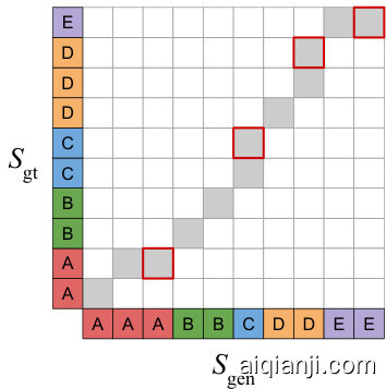
Figure 2: Dynamic time warping between two sequences finds a minimal-cost alignment path. Positions where warping occurs are marked with a border.
图 2: 两条序列间的动态时间规整 (Dynamic Time Warping) 寻找最小成本对齐路径。发生规整的位置用边框标出。
2.6 ALIGNER LENGTH LOSS
2.6 ALIGNER 长度损失
To ensure that the model produces realistic token length predictions, we add a loss which encourages the predicted utterance length to be close to the ground truth length. This length is found by summing all token length predictions. Let $L$ be the the number of time steps in the training utterance at $200\mathrm{Hz}$ , $l_{n}$ the predicted length of the $n$ th token, and $N$ the number of tokens, then the length loss is:
为确保模型生成真实的token长度预测,我们添加了一项损失函数,促使预测的语句长度接近真实长度。该长度通过累加所有token长度预测值得出。设$L$为训练语句在$200\mathrm{Hz}$下的时间步数,$l_{n}$为第$n$个token的预测长度,$N$为token总数,则长度损失函数为:
$$
\begin{array}{r}{\mathcal{L}_ {\mathrm{length}}=\frac{1}{2}\left(L-\sum_{n=1}^{N}l_{n}\right)^{2}.}\end{array}
$$
$$
\begin{array}{r}{\mathcal{L}_ {\mathrm{length}}=\frac{1}{2}\left(L-\sum_{n=1}^{N}l_{n}\right)^{2}.}\end{array}
$$
We use a scale factor $\lambda_{\mathrm{length}}=0.1$ . Note that we cannot match the predicted lengths $l_{n}$ to the ground truth lengths individually, because the latter are not available.
我们使用比例因子 $\lambda_{\mathrm{length}}=0.1$。需要注意的是,我们无法将预测长度 $l_{n}$ 与真实长度逐一匹配,因为后者不可用。
2.7 TEXT PRE-PROCESSING
2.7 文本预处理
Although our model works well with character input, we find that sample quality improves significantly using phoneme input instead. This is not too surprising, given the heterogeneous way in which spellings map to phonemes, particularly in the English language. Many character sequences also have special pronunciations, such as numbers, dates, units of measurement and website domains, and a very large training dataset would be required for the model to learn to pronounce these correctly. Text normalisation (Zhang et al., 2019) can be applied beforehand to spell out these sequences as they are typically pronounced (e.g., 1976 could become nineteen seventy six), potentially followed by conversion to phonemes. We use an open source tool, phonemizer (Bernard, 2020), which performs partial normalisation and phone mis ation (see Appendix F). Finally, whether we train on text or phoneme input sequences, we pre- and post-pad the sequence with a special silence token (for training and inference), to allow the aligner to account for silence at the beginning and end of each utterance.
虽然我们的模型在处理字符输入时表现良好,但我们发现使用音素输入能显著提升样本质量。考虑到拼写与音素间存在非固定映射关系(尤其是英语),这一结果并不令人意外。许多字符序列还存在特殊发音规则,例如数字、日期、计量单位和网站域名,要让模型学会正确发音需要极其庞大的训练数据集。文本归一化(Zhang et al., 2019)可预先将这些序列展开为常规发音形式(如将1976转换为nineteen seventy six),随后再转换为音素。我们采用开源工具phonemizer(Bernard, 2020)进行部分归一化和音素转换(详见附录F)。最后,无论训练文本还是音素输入序列,我们都会在序列首尾添加特殊静音token(用于训练和推理),使对齐器能够处理语句首尾的静音段。
3 RELATED WORK
3 相关工作
Speech generation saw significant quality improvements once treating it as a generative modelling problem became the norm (Zen et al., 2009; van den Oord et al., 2016). Likelihood-based approaches dominate, but generative adversarial networks (GANs) (Goodfellow et al., 2014) have been making significant inroads recently. A common thread through most of the literature is a separation of the speech generation process into multiple stages: coarse-grained temporally aligned intermediate representations, such as mel-spec tro grams, are used to divide the task into more manageable subproblems. Many works focus exclusively on either spec tr ogram generation or vocoding (generating a waveform from a spec tr ogram). Our work is different in this respect, and we will point out which stages of the generation process are addressed by each model. In Appendix J, Table 6 we compare these methods in terms of the inputs and outputs to each stage of their pipelines.
语音生成在将其视为生成式建模问题成为常态后(Zen et al., 2009; van den Oord et al., 2016),质量得到了显著提升。基于似然的方法占主导地位,但生成对抗网络(GANs)(Goodfellow et al., 2014)最近取得了重大进展。大多数文献的共同点是将语音生成过程分为多个阶段:使用粗粒度时间对齐的中间表示(如梅尔频谱图)将任务分解为更易处理的子问题。许多工作专门关注频谱图生成或声码器(从频谱图生成波形)。我们的工作在这方面有所不同,我们将指出每个模型处理生成过程的哪些阶段。在附录J的表6中,我们比较了这些方法在流程各阶段输入输出方面的差异。
Initially, most likelihood-based models for TTS were auto regressive (van den Oord et al., 2016; Mehri et al., 2017; Arik et al., 2017), which means that there is a sequential dependency between subsequent time steps of the produced output signal. That makes these models impractical for real-time use, although this can be addressed with careful engineering (Kal ch brenner et al., 2018; Valin & Skoglund, 2019). More recently, flow-based models (Papa makarios et al., 2019) have been explored as a feed-forward alternative that enables fast inference (without sequential dependencies). These can either be trained directly using maximum likelihood (Prenger et al., 2019; Kim et al., 2019; Ping et al., 2019b), or through distillation from an auto regressive model (van den Oord et al., 2018; Ping et al., 2019a). All of these models produce waveforms conditioned on an intermediate representation: either spec tro grams or “linguistic features”, which contain temporally-aligned high-level information about the speech signal. Spec tr ogram-conditioned waveform models are often referred to as vocoders.
最初,大多数基于似然的文本转语音(TTS)模型都是自回归的(van den Oord等人,2016;Mehri等人,2017;Arik等人,2017),这意味着生成输出信号的后续时间步之间存在顺序依赖性。这使得这些模型难以实时应用,尽管通过精心设计可以解决这一问题(Kalchbrenner等人,2018;Valin & Skoglund,2019)。最近,基于流的模型(Papamakarios等人,2019)作为一种前馈替代方案被探索,能够实现快速推理(无需顺序依赖)。这些模型可以直接通过最大似然训练(Prenger等人,2019;Kim等人,2019;Ping等人,2019b),或通过自回归模型蒸馏得到(van den Oord等人,2018;Ping等人,2019a)。所有这些模型都基于中间表示生成波形:要么是声谱图,要么是包含语音信号时间对齐高层信息的"语言学特征"。基于声谱图的波形模型通常被称为声码器。
A growing body of work has applied GAN (Goodfellow et al., 2014) variants to speech synthesis (Donahue et al., 2019). An important advantage of adversarial losses for TTS is a focus on realism over diversity; the latter is less important in this setting. This enables a more efficient use of capacity compared to models trained with maximum likelihood. MelGAN (Kumar et al., 2019) and Parallel WaveGAN (Yamamoto et al., 2020) are adversarial vocoders, producing raw waveforms from mel-spec tro grams. Neekhara et al. (2019) predict magnitude spec tro grams from mel-spec tro grams. Most directly related to our work is GAN-TTS (Binkowski et al., 2020), which produces waveforms conditioned on aligned linguistic features, and we build upon that work.
越来越多的研究将GAN (Goodfellow等人,2014) 的变体应用于语音合成 (Donahue等人,2019)。对抗性损失在TTS中的一个重要优势是更注重真实性而非多样性,后者在此场景中相对次要。与基于最大似然训练的模型相比,这使得模型容量得到更高效的利用。MelGAN (Kumar等人,2019) 和Parallel WaveGAN (Yamamoto等人,2020) 是采用对抗训练的声码器,能够从梅尔频谱图生成原始波形。Neekhara等人 (2019) 则实现了从梅尔频谱图预测幅度频谱图。与本研究最直接相关的是GAN-TTS (Binkowski等人,2020),该工作基于对齐的语言特征生成波形,我们的研究正是在此基础上展开。
Another important line of work covers spec tr ogram generation from text. Such models rely on a vocoder to convert the spec tro grams into waveforms (for which one of the previously mentioned models could be used, or a traditional spec tr ogram inversion technique (Griffin & Lim, 1984)). Tacotron 1 & 2 (Wang et al., 2017; Shen et al., 2018), Deep Voice 2 & 3 (Gibiansky et al., 2017; Ping et al., 2018), Transformer TT S (Li et al., 2019), Flowtron (Valle et al., 2020), and VoiceLoop (Taigman et al., 2017) are auto regressive models that generate spec tro grams or vocoder features frame by frame. Guo et al. (2019) suggest using an adversarial loss to reduce exposure bias (Bengio et al., 2015; Ranzato et al., 2016) in such models. MelNet (Vasquez & Lewis, 2019) is auto regressive over both time and frequency. ParaNet (Peng et al., 2019) and FastSpeech (Ren et al., 2019) are nonauto regressive, but they require distillation (Hinton et al., 2015) from an auto regressive model. Recent flow-based approaches Flow-TTS (Miao et al., 2020) and Glow-TTS (Kim et al., 2020) are feedforward without requiring distillation. Most spec tr ogram generation models require training of a custom vocoder model on generated spec tro grams, because their predictions are imperfect and the vocoder needs to be able to compensate for this2. Note that some of these works also propose new vocoder architectures in tandem with spec tr ogram generation models.
另一项重要工作涉及从文本生成频谱图。这类模型依赖声码器将频谱图转换为波形(可使用前文提到的任一模型,或传统频谱图反转技术 (Griffin & Lim, 1984))。Tacotron 1 & 2 (Wang et al., 2017; Shen et al., 2018)、Deep Voice 2 & 3 (Gibiansky et al., 2017; Ping et al., 2018)、Transformer TTS (Li et al., 2019)、Flowtron (Valle et al., 2020) 和 VoiceLoop (Taigman et al., 2017) 是通过逐帧生成频谱图或声码器特征的自回归模型。Guo et al. (2019) 提出使用对抗损失来减少此类模型中的曝光偏差 (Bengio et al., 2015; Ranzato et al., 2016)。MelNet (Vasquez & Lewis, 2019) 在时间和频率维度上均为自回归。ParaNet (Peng et al., 2019) 和 FastSpeech (Ren et al., 2019) 为非自回归模型,但需要从自回归模型进行知识蒸馏 (Hinton et al., 2015)。近期基于流的 Flow-TTS (Miao et al., 2020) 和 Glow-TTS (Kim et al., 2020) 为前馈结构且无需蒸馏。多数频谱图生成模型需在生成频谱图上训练定制声码器,因其预测存在缺陷需声码器补偿2。需注意部分研究在提出频谱图生成模型时同步设计了新声码器架构。
Unlike all of the aforementioned methods, as highlighted in Appendix J, Table 6, our model is a single feed-forward neural network, trained end-to-end in a single stage, which produces waveforms given character or phoneme sequences, and learns to align without additional supervision from auxiliary sources (e.g. temporally aligned linguistic features from an external model) or teacher forcing. This simplifies the training process considerably. Char2wav (Sotelo et al., 2017) is finetuned end-to-end in the same fashion, but requires a pre-training stage with vocoder features used for intermediate supervision.
与附录J表6中强调的所有前述方法不同,我们的模型是一个单一的前馈神经网络,通过单阶段端到端训练,能够在给定字符或音素序列时生成波形,并且无需来自辅助源(例如外部模型的时间对齐语言特征)或教师强制(teacher forcing)的额外监督就能学习对齐。这大大简化了训练过程。Char2wav (Sotelo等人,2017)采用相同方式进行端到端微调,但需要以声码器特征作为中间监督的预训练阶段。
Spec tr ogram prediction losses have been used extensively for feed-forward audio prediction models (Yamamoto et al., 2019; 2020; Yang et al., 2020; Arık et al., 2018; Engel et al., 2020; Wang et al.,
频谱图预测损失已广泛应用于前馈音频预测模型 (Yamamoto et al., 2019; 2020; Yang et al., 2020; Arık et al., 2018; Engel et al., 2020; Wang et al.,
2019; Défossez et al., 2018). We note that the $L_{1}$ loss we use (along with (Défossez et al., 2018)), is comparatively simple, as spec tr ogram losses in the literature tend to have separate terms penalising magnitudes, log-magnitudes and phase components, each with their own scaling factors, and often across multiple resolutions. Dynamic time warping on spec tro grams is a component of many speech recognition systems (Sakoe, 1971; Sakoe & Chiba, 1978), and has also been used for evaluation of TTS systems (Sailor & Patil, 2014; Chevelu et al., 2015). Cuturi & Blondel (2017) proposed the soft version of DTW we use in this work as a differentiable loss function for time series models. Kim et al. (2020) propose Monotonic Alignment Search (MAS), which relates to DTW in that both use dynamic programming to implicitly align sequences for TTS. However, they have different goals: MAS finds the optimal alignment between the text and a latent representation, whereas we use DTW to relax the constraints imposed by our spec tr ogram prediction loss term. Several mechanisms have been proposed to exploit monotonic it y in tasks that require sequence alignment, including attention mechanisms (Graves, 2013; Zhang et al., 2018; Vasquez & Lewis, 2019; He et al., 2019; Raffel et al., 2017; Chiu & Raffel, 2018), loss functions (Graves et al., 2006; Graves, 2012) and search-based approaches (Kim et al., 2020). For TTS, incorporating this constraint has been found to help generalisation to long sequences (Battenberg et al., 2020). We incorporate monotonic it y by using an interpolation mechanism, which is cheap to compute because it is not recurrent (unlike many monotonic attention mechanisms).
2019; Défossez等人, 2018)。我们注意到,所使用的$L_{1}$损失函数(与(Défossez等人, 2018)一致)相对简单,因为文献中的频谱图损失通常包含分别惩罚幅度、对数幅度和相位分量的独立项,每项都有各自的缩放因子,且常在多分辨率下计算。频谱图的动态时间规整(DTW)是许多语音识别系统的组成部分(Sakoe, 1971; Sakoe & Chiba, 1978),也被用于TTS系统评估(Sailor & Patil, 2014; Chevelu等人, 2015)。Cuturi & Blondel (2017)提出了本文采用的软DTW版本,作为时序模型的可微损失函数。Kim等人(2020)提出的单调对齐搜索(MAS)与DTW相关,两者都使用动态规划隐式对齐TTS序列。但目标不同:MAS寻找文本与潜在表示之间的最优对齐,而我们用DTW放松频谱图预测损失项的约束。已有多种机制利用单调性处理序列对齐任务,包括注意力机制(Graves, 2013; Zhang等人, 2018; Vasquez & Lewis, 2019; He等人, 2019; Raffel等人, 2017; Chiu & Raffel, 2018)、损失函数(Graves等人, 2006; Graves, 2012)和基于搜索的方法(Kim等人, 2020)。在TTS中,这种约束有助于提升长序列泛化能力(Battenberg等人, 2020)。我们通过插值机制实现单调性,该机制计算成本低(与多数单调注意力机制不同)。
4 EVALUATION
4 评估
In this section we discuss the setup and results of our empirical evaluation, describing the hyperparameter settings used for training and validating the architectural decisions and loss function components detailed in Section 2. Our primary metric used to evaluate speech quality is the Mean Opinion Score (MOS) given by human raters, computed by taking the mean of 1-5 naturalness ratings given across 1000 held-out conditioning sequences. In Appendix I we also report the Fréchet DeepSpeech Distance (FDSD), proposed by Binkowski et al. (2020) as a speech synthesis quality metric. Appendix A reports training and evaluation hyper parameters we used for all experiments.
本节我们将讨论实证评估的设置与结果,详细说明用于训练的超参数配置以及验证第2章所述的架构决策与损失函数组件。评估语音质量的核心指标是人工评分者给出的平均意见得分(MOS),通过对1000条保留条件序列的1-5分自然度评分取均值计算得出。附录I还报告了由Binkowski等人(2020)提出的Fréchet DeepSpeech距离(FDSD)作为语音合成质量指标。附录A列出了所有实验采用的训练与评估超参数。
4.1 MULTI-SPEAKER DATASET
4.1 多说话人数据集
We train all models on a private dataset that consists of high-quality recordings of human speech performed by professional voice actors, and corresponding text. The voice pool consists of 69 female and male voices of North American English speakers, while the audio clips contain full sentences of lengths varying from less than 1 to 20 seconds at $24\mathrm{kHz}$ frequency. Individual voices are unevenly distributed, accounting for from 15 minutes to over 51 hours of recorded speech, totalling 260.49 hours. At training time, we sample 2 second windows from the individual clips, post-padding those shorter than 2 seconds with silence. For evaluation, we focus on the single most prolific speaker in our dataset, with all our main MOS results reported with the model conditioned on that speaker ID, but also report MOS results for each of the top four speakers using our main multi-speaker model.
我们在一个私有数据集上训练所有模型,该数据集包含专业配音演员录制的高质量人类语音及对应文本。语音库由69位北美英语母语者的男女声组成,音频片段为完整句子,时长从不足1秒到20秒不等,采样频率为$24\mathrm{kHz}$。个体语音数据分布不均,录制时长从15分钟到51小时以上不等,总计260.49小时。训练时,我们从单个片段中采样2秒窗口,对不足2秒的片段用静音进行后补零。评估时,我们聚焦数据集中产量最高的单一说话人,所有主要MOS(平均意见分)结果均基于该说话人ID的条件化模型得出,但同时也使用主多说话人模型报告了前四位说话人各自的MOS结果。
4.2 RESULTS
4.2 结果
In Table 1 we present quantitative results for our EATS model described in Section 2, as well as several ablations of the different model and learning signal components. The architecture and training setup of each ablation is identical to our base EATS model except in terms of the differences described by the columns in Table 1. Each ablation is “subtractive”, representing the full EATS system minus one particular feature. Our main result achieved by the base multi-speaker model is a mean opinion score (MOS) of 4.083. Although it is difficult to compare directly with prior results from the literature due to dataset differences, we nonetheless include MOS results from prior works (Binkowski et al. 2020; van den Oord et al., 2016; 2018), with MOS in the 4.2 to $4.4+$ range. Compared to these prior models, which rely on aligned linguistic features, EATS uses substantially less supervision.
在表1中,我们展示了第2节描述的EATS模型的定量结果,以及不同模型和学习信号组件的多项消融实验。每个消融实验的架构和训练设置与基础EATS模型完全相同,仅存在表1各列所描述的差异。所有消融实验均为"减法式",代表完整EATS系统减去某一特定功能。基础多说话人模型取得的主要成果是4.083的平均意见得分(MOS)。尽管由于数据集差异难以直接与文献中的先前结果比较,我们仍列出了先前工作(Binkowski等人2020;van den Oord等人2016;2018)的MOS结果,其得分在4.2至$4.4+$范围内。与这些依赖对齐语言特征的先前模型相比,EATS使用的监督信息显著减少。
The No RWDs, No MelSpecD, and No Disc rim in at or s ablations all achieved substantially worse MOS results than our proposed model, demonstrating the importance of adversarial feedback. In particular, the No RWDs ablation, with an MOS of 2.526, demonstrates the importance of the raw audio feedback, and removing RWDs significantly degrades the high frequency components. No MelSpecD causes intermittent artifacts and distortion, and removing all disc rim in at or s results in audio that sounds robotic and distorted throughout. The No $\mathcal{L}_ {\mathrm{length}}$ and No $\mathcal{L}_{\mathrm{pred}}$ ablations result in a model that does not train at all. Comparing our model with No DTW (MOS 3.559), the temporal flexibility provided by dynamic time warping significantly improves fidelity: removing it causes warbling and unnatural phoneme lengths. No Phonemes is trained with raw character inputs and attains MOS 3.423, due to occasional mispronunciations and unusual stress patterns. No Mon. Int. uses an aligner with a transformer-based attention mechanism (described in Appendix G) in place of our monotonic interpolation architecture, which turns out to generalise poorly to long utterances (yielding MOS 3.551). Finally, comparing against training with only a Single Speaker (MOS 3.829) shows that our EATS model benefits from a much larger multi-speaker dataset, even though MOS is evaluated only on this same single speaker on which the ablation was solely trained. Samples from each ablation are available at https://deepmind.com/research/publications/ End-to-End-Adversarial-Text-to-Speech.
无RWDs、无MelSpecD和无判别器的消融实验均比我们提出的模型获得了显著更差的MOS评分,这证明了对抗性反馈的重要性。特别是无RWDs消融实验(MOS 2.526)验证了原始音频反馈的关键作用,移除RWDs会显著劣化高频成分。无MelSpecD会导致间歇性伪影和失真,而移除所有判别器则会使音频全程呈现机械感与失真。无$\mathcal{L}_ {\mathrm{length}}$和无$\mathcal{L}_{\mathrm{pred}}$的消融实验会导致模型完全无法训练。将我们的模型与无DTW版本(MOS 3.559)对比表明,动态时间规整提供的时间灵活性显著提升了保真度:移除该功能会导致颤音现象和非自然音素长度。无音素版本使用原始字符输入训练,因偶发发音错误和异常重音模式获得MOS 3.423。无单调插值版本使用基于Transformer注意力机制的对齐器(附录G详述)替代我们的单调插值架构,该方案对长语句泛化能力较差(MOS 3.551)。最后,与单说话人训练(MOS 3.829)的对比表明,我们的EATS模型受益于更大的多说话人数据集,尽管MOS评估仅针对消融实验训练所用的同一说话人。各消融实验样本详见https://deepmind.com/research/publications/End-to-End-Adversarial-Text-to-Speech。
Table 1: Mean Opinion Scores (MOS) for our final EATS model and the ablations described in Section 4, sorted by MOS. The middle columns indicate which components of our final model are enabled or ablated. Data describes the training set as Multi speaker (MS) or Single Speaker (SS). Inputs describes the inputs as raw characters $\mathrm{(Ch)}$ or phonemes $\mathrm{(Ph)}$ produced by Phonemizer. RWD (Random Window Disc rim in at or s), $M S D$ (Mel-spec tr ogram Disc rim in at or), and $\mathcal{L}_ {\mathrm{length}}$ (length prediction loss) indicate the presence $(\checkmark)$ or absence $(\times)$ of each of these training components described in Section 2. $\mathcal{L}_ {\mathrm{pred}}$ indicates which spec tr ogram prediction loss was used: with DTW $(\mathcal{L}_ {\mathrm{pred}}^{\prime\prime}$ , Eq. 6), without DTW $\mathcal{L}_{\mathrm{pred}}$ , Eq. 3), or absent $(\times)$ . Align describes the architecture of the aligner as monotonic interpolation (MI) or attention-based (Attn). We also compare against recent state-of-the-art approaches from the literature which are trained on aligned linguistic features (unlike our models). Our MOS evaluation set matches that of GAN-TTS (Binkowski et al., 2020) (and our “Single Speaker” training subset matches the GAN-TTS training set); the other approaches are not directly comparable due to dataset differences.
| Model | Data Inputs | RWD | MSD | Llength Lpred | Align | MOS | |
| Natural Speech | 4.55 ± 0.075 | ||||||
| GAN-TTS (Binkowskiet al.,2020) | 4.213 ± 0.046 | ||||||
| WaveNet(vandenOordetal.,2016) | 4.41 ± 0.069 | ||||||
| Par:WaveNet(van den Oord et al.,2018) | 4.41 ± 0.078 | ||||||
| Tacotron2 (Shenet al.,2018) | 4.526 ±0.066 | ||||||
| No Llength | MS | Ph | × | MI | [does not train] | ||
| No Lpred | MS | Ph | MI | [does not train] | |||
| NoDiscriminators | MS | Ph | √ × | C" pred | MI | 1.407 ± 0.040 | |
| No RWDs | MS | Ph | MI | 2.526 ±0.060 | |||
| No Phonemes | MS | Ch | pred | MI | 3.423±0.073 | ||
| No MelSpecD | MS | Ph | MI | 3.525 ±0.057 | |||
| No Mon. Int. | MS | Ph | 'pred | Attn | 3.551±0.073 | ||
| NoDTW | MS | Ph | Lpred | MI | 3.559 ± 0.065 | ||
| Single Speaker | SS | Ph | MI | 3.829 ± 0.055 | |||
| EATS (Ours) | MS | Ph | √ | Clpred MI | 4.083 ± 0.049 |
表 1: 最终EATS模型及各消融实验的平均意见得分(MOS),按MOS排序。中间列表示最终模型中启用或消融的组件。"Data"描述训练集为多说话人(MS)或单说话人(SS)。"Inputs"描述输入为原始字符$\mathrm{(Ch)}$或由Phonemizer生成的音素$\mathrm{(Ph)}$。RWD(随机窗口判别器)、$MSD$(梅尔谱判别器)和$\mathcal{L}_ {\mathrm{length}}$(长度预测损失)表示这些训练组件的存在$(\checkmark)$或缺失$(\times)$。$\mathcal{L}_ {\mathrm{pred}}$表示使用的谱图预测损失类型:带DTW的$(\mathcal{L}_ {\mathrm{pred}}^{\prime\prime}$,公式6)、不带DTW的($\mathcal{L}_{\mathrm{pred}}$,公式3)或缺失$(\times)$。"Align"描述对齐器架构为单调插值(MI)或基于注意力机制(Attn)。我们还与文献中使用对齐语言学特征的最新方法进行了对比(与我们的模型不同)。我们的MOS评估集与GAN-TTS(Binkowski等人,2020)一致(且"单说话人"训练子集与GAN-TTS训练集匹配);由于数据集差异,其他方法不具备直接可比性。
| 模型 | 数据输入 | RWD | MSD | $\mathcal{L}_ {\mathrm{length}}$ $\mathcal{L}_ {\mathrm{pred}}$ | 对齐方式 | MOS |
|---|---|---|---|---|---|---|
| 自然语音 | - | - | - | - | - | 4.55 ± 0.075 |
| GAN-TTS (Binkowski等人,2020) | - | - | - | - | - | 4.213 ± 0.046 |
| WaveNet(van den Oord等人,2016) | - | - | - | - | - | 4.41 ± 0.069 |
| Parallel WaveNet(van den Oord等人,2018) | - | - | - | - | - | 4.41 ± 0.078 |
| Tacotron2 (Shen等人,2018) | - | - | - | - | - | 4.526 ±0.066 |
| 无长度损失 | MS | Ph | × | - | MI | [不训练] |
| 无预测损失 | MS | Ph | - | × | MI | [不训练] |
| 无判别器 | MS | Ph | × | × | $\mathcal{L}_{\mathrm{pred}}^{\prime\prime}$ | MI |
| 无RWD | MS | Ph | × | √ | $\mathcal{L}_{\mathrm{pred}}$ | MI |
| 无音素 | MS | Ch | √ | √ | $\mathcal{L}_{\mathrm{pred}}$ | MI |
| 无梅尔谱判别器 | MS | Ph | √ | × | $\mathcal{L}_{\mathrm{pred}}$ | MI |
| 无单调插值 | MS | Ph | √ | √ | $\mathcal{L}_{\mathrm{pred}}^{\prime}$ | Attn |
| 无DTW | MS | Ph | √ | √ | $\mathcal{L}_{\mathrm{pred}}$ | MI |
| 单说话人 | SS | Ph | √ | √ | $\mathcal{L}_{\mathrm{pred}}^{\prime\prime}$ | MI |
| EATS (本文) | MS | Ph | √ | √ | $\mathcal{L}_{\mathrm{pred}}^{\prime\prime}$ | MI |
Table 2: Mean Opinion Scores (MOS) for the top four speakers with the most data in our training set. All evaluations are done using our single multi-speaker EATS model.
| Speaker | #1 | #2 | #3 | #4 |
| Speaking Time (Hours) | 51.68 | 31.21 | 20.68 | 10.32 |
| MOS | 4.083 ± 0.049 | 3.828± 0.051 | 4.149 ± 0.045 | 3.761± 0.052 |
表 2: 训练集中数据量最多的四位说话人的平均意见得分(MOS)。所有评估均使用我们的单一多说话人EATS模型完成。
| Speaker | #1 | #2 | #3 | #4 |
|---|---|---|---|---|
| Speaking Time (Hours) | 51.68 | 31.21 | 20.68 | 10.32 |
| MOS | 4.083 ± 0.049 | 3.828± 0.051 | 4.149 ± 0.045 | 3.761± 0.052 |
We demonstrate that the aligner learns to use the latent vector $\mathbf{z}$ to vary the predicted token lengths in Appendix H. In Table 2 we present additional MOS results from our main multi-speaker EATS model for the four most prolific speakers in our training data3. MOS generally improves with more training data, although the correlation is imperfect (e.g., Speaker #3 achieves the highest MOS with only the third most training data).
我们证明对齐器学会了利用潜在向量$\mathbf{z}$来改变预测的token长度(详见附录H)。在表2中,我们展示了主多说话人EATS模型中训练数据量最大的四位说话人的额外MOS结果。虽然相关性并不完美(例如说话人#3仅用第三多的训练数据就获得了最高MOS),但MOS通常随着训练数据的增加而提升。
5 DISCUSSION
5 讨论
We have presented an adversarial approach to text-to-speech synthesis which can learn from a relatively weak supervisory signal – normalised text or phonemes paired with corresponding speech audio. The speech generated by our proposed model matches the given conditioning texts and general is es to unobserved texts, with naturalness judged by human raters approaching state-of-the-art systems with multi-stage training pipelines or additional supervision. The proposed system described in Section 2 is efficient in both training and inference. In particular, it does not rely on auto regressive sampling or teacher forcing, avoiding issues like exposure bias (Bengio et al., 2015; Ranzato et al., 2016) and reduced parallelism at inference time, or the complexities introduced by distillation to a more efficient feed-forward model after the fact (van den Oord et al., 2018; Ping et al., 2019a).
我们提出了一种对抗式文本转语音合成方法,该方法能够从相对较弱的监督信号(规范化文本或音素与对应语音音频配对)中学习。我们提出的模型生成的语音与给定条件文本相匹配,并能泛化到未见过的文本,其自然度经人类评估接近采用多阶段训练流程或额外监督的最先进系统。第2节描述的该系统在训练和推理阶段均高效,尤其不依赖自回归采样或教师强制,避免了推理时的曝光偏差问题(Bengio等人,2015;Ranzato等人,2016)和并行性降低,也无需事后通过蒸馏简化成前馈模型(van den Oord等人,2018;Ping等人,2019a)所带来的复杂性。
While there remains a gap between the fidelity of the speech produced by our method and the stateof-the-art systems, we nonetheless believe that the end-to-end problem setup is a promising avenue for future advancements and research in text-to-speech. End-to-end learning enables the system as a whole to benefit from large amounts of training data, freeing models to optimise their intermediate representations for the task at hand, rather than constraining them to work with the typical bottlenecks (e.g., mel-spec tro grams, aligned linguistic features) imposed by most TTS pipelines today. We see some evidence of this occurring in the comparison between our main result, trained using data from 69 speakers, against the Single Speaker ablation: the former is trained using roughly four times the data and synthesis es more natural speech in the single voice on which the latter is trained.
尽管我们的方法生成的语音保真度与最先进的系统之间仍存在差距,但我们认为端到端的问题设置是未来文本转语音技术发展和研究的一条有前景的路径。端到端学习使整个系统能够从大量训练数据中受益,释放模型优化其中间表示的能力,以适应当前任务,而不是限制它们使用当今大多数TTS流程中常见的瓶颈(例如梅尔频谱图、对齐的语言学特征)。我们在主要结果(使用69位说话人的数据进行训练)与单说话人消融实验的对比中看到了这一点的证据:前者使用了大约四倍的数据进行训练,并在后者训练的单一语音上合成了更自然的语音。
Notably, our current approach does not attempt to address the text normalisation and phone mis ation problems, relying on a separate, fixed system for these aspects, while a fully end-to-end TTS system could operate on un normal is ed raw text. We believe that a fully data-driven approach could ultimately prevail even in this setup given sufficient training data and model capacity.
值得注意的是,我们当前的方法并未尝试解决文本归一化(text normalisation)和音素错误(phone mis)问题,而是依赖一个独立的固定系统来处理这些方面,而一个完全端到端的TTS系统可以直接处理未归一化的原始文本。我们相信,只要有足够的训练数据和模型容量,完全数据驱动的方法最终也能在这种设定下取得优势。
ACKNOWLEDGMENTS
致谢
The authors would like to thank Norman Casagrande, Yutian Chen, Aidan Clark, Kazuya Kawakami, Pauline Luc, and many other colleagues at DeepMind for valuable discussions and input.
作者感谢Norman Casagrande、Yutian Chen、Aidan Clark、Kazuya Kawakami、Pauline Luc以及DeepMind的其他同事提供的宝贵讨论与意见。
Andrew Gibiansky, Sercan Arik, Gregory Diamos, John Miller, Kainan Peng, Wei Ping, Jonathan Raiman, and Yanqi Zhou. Deep Voice 2: Multi-speaker neural text-to-speech. In NeurIPS, 2017.
Andrew Gibiansky、Sercan Arik、Gregory Diamos、John Miller、Kainan Peng、Wei Ping、Jonathan Raiman 和 Yanqi Zhou。Deep Voice 2: 多说话人神经文本到语音。发表于 NeurIPS,2017。
Ian Goodfellow, Jean Pouget-Abadie, Mehdi Mirza, Bing Xu, David Warde-Farley, Sherjil Ozair, Aaron Courville, and Yoshua Bengio. Generative adversarial nets. In NeurIPS, 2014.
Ian Goodfellow、Jean Pouget-Abadie、Mehdi Mirza、Bing Xu、David Warde-Farley、Sherjil Ozair、Aaron Courville 和 Yoshua Bengio。生成对抗网络。发表于 NeurIPS,2014。
Table 3: EATS batched inference benchmarks, timing inference (speech generation) on a Google Cloud TPU v3 (1 chip with 2 cores), a single NVIDIA V100 GPU, or an Intel Xeon E5-1650 v4 CPU at $3.60\mathrm{GHz}$ (6 physical cores). We use a batch size of 2, 8, or 16 utterances (Utt.), each 30 seconds long (input length of 600 phoneme tokens, padded if necessary). One “run” consists of 10 consecutive forward passes at the given batch size. We perform 101 such runs and report the median run time (Med. Run Time (s)) and the resulting Realtime Factor, the ratio of the total duration of the generated speech (Length / Run (s)) to the run time. (Note: GPU benchmarking is done using single precision (IEEE FP32) floating point; switching to half precision (IEEE FP16) could yield further speedups.)
| Hardware | #Utt./ Batch | #Batch/ Run | #Utt./ Run | Length / Utt. (s) | Length / Run (s) | Med.Run Time (s) | Realtime Factor |
| TPU v3 (1 chip) | 16 | 10 | 160 | 30 | 4800 | 30.53 | 157.2x |
| V100 GPU (1) | 8 | 10 | 80 | 30 | 2400 | 11.60 | 206.8x |
| Xeon CPU (6 cores) | 2 | 10 | 20 | 30 | 600 | 70.42 | 8.520x |
表 3: EATS 批量推理基准测试,分别在 Google Cloud TPU v3 (1 个芯片含 2 核)、单个 NVIDIA V100 GPU 或 Intel Xeon E5-1650 v4 CPU ($3.60\mathrm{GHz}$,6 物理核) 上进行语音生成时序推理。采用 2、8 或 16 条话语 (Utt.) 的批量大小,每条时长 30 秒 (输入为 600 个音素 token,不足时填充)。每次"运行"包含给定批量下的 10 次连续前向传播。我们执行 101 次此类运行并报告中位运行时间 (Med. Run Time (s)) 及由此得出的实时因子 (生成语音总时长 (Length / Run (s)) 与运行时间的比值)。(注: GPU 基准测试使用单精度 (IEEE FP32) 浮点运算;切换为半精度 (IEEE FP16) 可能获得额外加速。)
| 硬件 | 每批话语数 | 每轮批次数 | 每轮话语数 | 单话语时长 (s) | 单轮总时长 (s) | 中位运行时间 (s) | 实时因子 |
|---|---|---|---|---|---|---|---|
| TPU v3 (1芯片) | 16 | 10 | 160 | 30 | 4800 | 30.53 | 157.2x |
| V100 GPU (1个) | 8 | 10 | 80 | 30 | 2400 | 11.60 | 206.8x |
| Xeon CPU (6核) | 2 | 10 | 20 | 30 | 600 | 70.42 | 8.520x |
A HYPER PARAMETERS AND OTHER DETAILS
超参数及其他细节
Our models are trained for $5\cdot10^{5}$ steps, where a single step consists of one disc rim in at or update followed by one generator update, each using a minibatch size of 1024, with batches sampled independently in each of these two updates. Both updates are computed using the Adam optimizer (Kingma & Ba, 2015) with $\beta_{1}=0$ and $\beta_{2}=0.999$ , and a learning rate of $10^{-3}$ with a cosine decay (Loshchilov & Hutter, 2017) schedule used such that the learning rate is 0 at step 500K. We apply spectral normalisation (Miyato et al., 2018) to the weights of the generator’s decoder module and to the disc rim in at or s (but not to the generator’s aligner module). Parameters are initial is ed orthogonal ly and off-diagonal orthogonal regular is ation with weight $10^{-4}$ is applied to the generator, following BigGAN (Brock et al., 2018). Mini batches are split over 64 or 128 cores (32 or 64 chips) of Google Cloud TPU v3 Pods, which allows training of a single model within up to 58 hours. We use crossreplica BatchNorm (Ioffe & Szegedy, 2015) to compute batch statistics aggregated across all devices. Like in GAN-TTS (Binkowski et al., 2020), our trained generator requires computation of standing statistics before sampling; i.e., accumulating batch norm statistics from 200 forward passes. As in GAN-TTS (Binkowski et al., 2020) and BigGAN (Brock et al., 2018), we use an exponential moving average of the generator weights for inference, with a decay of 0.9999. Although GANs are known to exhibit stability issues sometimes, we found that EATS model training consistently converges.
我们的模型训练了 $5\cdot10^{5}$ 步,其中每一步包含一次判别器更新和一次生成器更新,每次更新使用1024的小批量(minibatch)数据,且这两次更新的批次数据独立采样。两次更新均采用Adam优化器 (Kingma & Ba, 2015),参数设为 $\beta_{1}=0$ 和 $\beta_{2}=0.999$,初始学习率为 $10^{-3}$ 并采用余弦衰减 (Loshchilov & Hutter, 2017) 调度,使得第50万步时学习率降为0。我们对生成器解码器模块和判别器的权重应用谱归一化 (Miyato et al., 2018)(但不包括生成器的对齐模块)。参数初始化采用正交矩阵,并参照BigGAN (Brock et al., 2018) 对生成器施加权重为 $10^{-4}$ 的非对角正交正则化。小批量数据在Google Cloud TPU v3 Pod的64或128个核心(32或64个芯片)上并行处理,单个模型训练时间最长不超过58小时。我们使用跨副本批归一化 (Ioffe & Szegedy, 2015) 计算跨设备聚合的批次统计量。与GAN-TTS (Binkowski et al., 2020) 类似,训练后的生成器在采样前需计算静态统计量,即通过200次前向传播累积批归一化统计量。参照GAN-TTS (Binkowski et al., 2020) 和BigGAN (Brock et al., 2018),推理时采用生成器权重的指数移动平均,衰减率为0.9999。尽管GAN模型存在稳定性问题,但我们发现EATS模型的训练始终能稳定收敛。
Models were implemented using TensorFlow (Abadi et al., 2015) v1 framework and the Sonnet (Reynolds et al., 2017) neural network library. We used the TF-Replicator (Buchlovsky et al., 2019) library for data parallel training over TPUs.
模型使用 TensorFlow (Abadi et al., 2015) v1 框架和 Sonnet (Reynolds et al., 2017) 神经网络库实现。我们采用 TF-Replicator (Buchlovsky et al., 2019) 库在 TPU 上进行数据并行训练。
Inference speed. In Table 3 we report benchmarks for EATS batched inference on two modern hardware platforms (Google Cloud TPU v3, NVIDIA V100 GPU, Intel Xeon E5-1650 CPU). We find that EATS can generate speech two orders of magnitude faster than realtime on a GPU or TPU, demonstrating the efficiency of our feed-forward model. On the GPU, generating 2400 seconds (40 minutes) of speech (80 utterances of 30 seconds each) takes 11.60 seconds on average (median), for a realtime factor of $206.8\times$ . On TPU we observe a realtime factor of $157.2\times$ per chip (2 cores), or $78.6\times$ per core. On a CPU, inference runs at $8.52\times$ realtime.
推理速度。表3展示了EATS在两个现代硬件平台(Google Cloud TPU v3、NVIDIA V100 GPU、Intel Xeon E5-1650 CPU)上的批量推理基准测试结果。我们发现EATS在GPU或TPU上的语音生成速度比实时快两个数量级,这证明了我们前馈模型的高效性。在GPU上,生成2400秒(40分钟)的语音(80段30秒的语句)平均耗时11.60秒(中位数),实时系数为$206.8\times$。在TPU上,我们观察到每芯片(2核)的实时系数为$157.2\times$,即每核$78.6\times$。在CPU上,推理速度为$8.52\times$实时。
B ALIGNER PSEUDOCODE
B ALIGNER 伪代码
In Figure 3 we present pseudocode for the EATS aligner described in Section 2.1.
图 3: 我们展示了第 2.1 节中描述的 EATS aligner 的伪代码。
C SPEC TR OGRAM DISC RIM IN AT OR ARCHITECTURE
C SPEC TR OGRAM DISC RIM IN AT OR 架构
In this Appendix we present details of the architecture of the spec tr ogram disc rim in at or (Section 2.3). The disc rim in at or’s inputs are $47\times80\times1$ images, produced by adding a channel dimension to the $47\times80$ output of the mel-spec tr ogram computation (Appendix D) from the length 48000 input waveforms (2 seconds of audio at $24\mathrm{kHz}$ ).
在本附录中,我们将详细介绍频谱图判别器(见第2.3节)的架构。判别器的输入为$47\times80\times1$的图像,这些图像是通过对梅尔频谱图计算(附录D)输出的$47\times80$矩阵添加通道维度得到的,原始输入为长度48000的波形(24kHz采样率下2秒的音频)。
Then, the architecture is like that of the BigGAN-deep (Brock et al., 2018) disc rim in at or for $128\times128$ images (listed in BigGAN (Brock et al., 2018) Appendix B, Table 7 (b)), but removing the first two “ResBlocks” and the “Non-Local Block” (self-attention) – rows 2-4 in the architecture table (keeping row 1, the input convolution, and rows $^{5+}$ afterwards, as is). This removes one $2\times2$ down sampling step as the resolution of the spec tr ogram inputs is smaller than the $128\times128$ images for which the BigGAN-deep architecture was designed. We set the channel width multiplier referenced in the table to $c h=64$ .
随后,该架构类似于BigGAN-deep (Brock et al., 2018) 中针对$128\times128$图像的判别器(列于BigGAN (Brock et al., 2018)附录B的表7(b)),但移除了前两个"ResBlocks"和"Non-Local Block"(自注意力机制)——即架构表中第2-4行(保留第1行输入卷积层及第$^{5+}$行之后的原始结构)。由于频谱图输入的尺寸小于BigGAN-deep架构设计的$128\times128$图像,这一调整减少了一个$2\times2$下采样步骤。我们将表中引用的通道宽度乘数设置为$ch=64$。
Returns:
返回:
aligned features: audio-aligned features to be fed into the decoder. (dtype=float, shape=[N, out sequence length, 256]) aligned lengths: the predicted audio-aligned lengths. (dtype=float, shape=[N])
对齐特征 (aligned features):输入解码器的音频对齐特征。(数据类型=浮点型,维度=[N, 输出序列长度, 256])
对齐长度 (aligned lengths):预测的音频对齐长度。(数据类型=浮点型,维度=[N])
#Make the "class-conditioning" inputs for class-conditional batch norm (CCBN)
#using the embedded speaker IDs and the noise.
ccbn_condition = Concat([embedded_speaker_ids, noise], axis=1) #-> [N, 256]
#Add a dummy sequence axis to ccbn_condition for broadcasting.
ccbn_condition = ccbn_condition[:, None, :] #-> [N, 1, 256]
#为类别条件批归一化 (CCBN) 创建"类别条件"输入
#使用嵌入的说话人ID和噪声。
ccbn_condition = Concat([embedded_speaker_ids, noise], axis=1)#-> [N, 256]
#为广播添加虚拟序列轴到c_cbn_condition。
ccbn_condition = ccbn_condition[:, None, :] #-> [N, 1, 256]
#Use lengths to make a mask indicating valid entries of token_sequences.
sequence_length = token_sequences.shape[1] # = 600
mask = Range(sequence_length)[None, :] < lengths[:, None] #-> [N, 600]
#使用 `lengths` 创建掩码以标记 token 序列的有效条目。序列长度 = token sequences.shape[1] #=600
掩码 Range(sequence_length)[None, :] < lengths[:, None] #-> [N, 600]
#Dilated 1D convolution stack.
#扩张一维卷积堆栈
#Save dilated conv stack outputs as un aligned features. un aligned features $=\times$ # [N, 600, 256]
将膨胀卷积堆栈输出保存为未对齐特征。未对齐特征 $=\times$ # [N, 600, 256]
#Map to predicted token lengths.
#映射到预测的token长度。
#Compute output grid $\begin {array} {r l} {->}& {{}\int N,}\end {array}$ out sequence length=6000] out_pos $=$ Range(out sequence length)[None, :] $^+$ out_offset[:, None] out_pos $=$ Cast(out_pos[:, :, None], float) # -> [N, 6000, 1] diff = token centres[:, None, :] - out_pos # -> [N, 6000, 600] logits $=$ -(diff**2 / sigma2) # -> [N, 6000, 600] $#$ Mask out invalid input locations (flip 0/1 to 1/0); add dummy output axis. log its in v mask $=_1$ . - Cast(mask[:, None, :], float) # -> [N, 1, 600] masked log its $=$ logits - 1e9 * log its in v mask # -> [N, 6000, 600] weights = Softmax(masked log its, axis $=2$ ) # -> [N, 6000, 600] # Do a batch matmul (written as an einsum) to compute the aligned features. # aligned_features -> [N, 6000, 256] aligned features $=$ Einsum('noi,nid->nod', weights, un aligned features)
#计算输出网格 $\begin {array} {r l} {->}& {{}\int N,}\end {array}$ 输出序列长度=6000]
out_pos $=$ Range(输出序列长度)[None, :] $^+$ out_offset[:, None]
out_pos $=$ Cast(out_pos[:, :, None], float) # -> [N, 6000, 1]
diff = token中心点[:, None, :] - out_pos # -> [N, 6000, 600]
logits $=$ -(diff**2 / sigma2) # -> [N, 6000, 600]
#掩码无效输入位置(将0/1翻转为1/0);添加虚拟输出轴
logits_inv_mask $=1$ - Cast(mask[:, None, :], float) # -> [N, 1, 600]
masked_logits $=$ logits - 1e9 * logits_inv_mask # -> [N, 6000, 600]
weights = Softmax(masked_logits, axis $=2$) # -> [N, 6000, 600]
#执行批量矩阵乘法(写作einsum形式)计算对齐特征
#aligned_features -> [N, 6000, 256]
aligned_features $=$ Einsum('noi,nid->nod', weights, unaligned_features)
return aligned features, aligned lengths
返回对齐特征、对齐长度
#import tensorflow.compat.v1 as tf
#import tensorflow.compat.v1 as tf
def get mel spec tr ogram(waveforms, invert mu law $=$ True, mu=255., jitter=False, max j it ter step $\mathfrak{z}=60$ ): """Computes mel-spec tro grams for the given waveforms. Args: waveforms: a tf.Tensor corresponding to a batch of waveforms sampled at 24 kHz. (dtype=tf.float32, shape $=$ [N, sequence length]) invert mu law: whether to apply mu-law inversion to the input waveforms. In EATS both the real data and generator outputs are mu-law'ed, so this is always set to True. mu: The mu value used if invert mu law $=$ True (ignored otherwise). jitter: whether to apply random jitter to the input waveforms before computing spec tro grams. Set to True only for GT spec tro grams input to the prediction loss. max j it ter steps: maximum number of steps by which the input waveforms are randomly jittered if jitte $?=$ True (ignored otherwise).
def get_mel_spectrogram(waveforms, invert_mu_law=True, mu=255., jitter=False, max_jitter_step=60):
"""为给定波形计算梅尔频谱图。
参数:
waveforms: 对应24kHz采样波形批次的tf.Tensor (dtype=tf.float32, shape=[N, 序列长度])
invert_mu_law: 是否对输入波形应用μ律逆变换。在EATS中真实数据和生成器输出都经过μ律压缩,因此该参数始终设为True。
mu: 当invert_mu_law=True时使用的μ值(否则忽略)。
jitter: 在计算频谱图前是否对输入波形施加随机抖动。仅在预测损失的GT频谱图输入时设为True。
max_jitter_steps: 当jitter=True时输入波形随机抖动的最大步数(否则忽略)。
Returns:
返回:
A 3D tensor with spec tro grams for the corresponding input waveforms (dtype $=$ tf.float32, shape $=$ [N, num_frames=ceil(sequence length/1024), num_bin $\mathfrak{s}=\mathcal{B}\mathcal{O}\mathcal{J}$ )
一个3D张量,包含对应输入波形的频谱图 (dtype $=$ tf.float32, shape $=$ [N, num_frames=ceil(sequence length/1024), num_bin $\mathfrak{s}=\mathcal{B}\mathcal{O}\mathcal{J}$ )
"""
"""
waveforms.shape.assert has rank(2) t $=$ waveforms
波形形状断言具有秩(2) t $=$ 波形
if jitter:
如果存在抖动:
D MEL-SPEC TR OGRAM COMPUTATION
D MEL-SPEC TR OGRAM 计算
In Figure 4 we include the TensorFlow (Abadi et al., 2015) code used to compute the mel-spec tro grams fed into the spec tr ogram disc rim in at or (Section 2.3) and the spec tr ogram prediction loss (Section 2.4). Note that for use in the prediction losses $\mathcal{L}_ {\mathrm{pred}}$ or $\mathcal{L}_{\mathrm{pred}}^{\prime\prime}$ , we call this function with jitter $=$ True for real spec tro grams and jitter $=$ False for generated spec tro grams. When used for the spectrogram disc rim in at or inputs, we do not apply jitter to either real or generated spec tro grams, setting jitter $=$ False in both cases.
在图4中,我们包含了用于计算输入频谱图判别器 (见2.3节) 和频谱图预测损失 (见2.4节) 的梅尔频谱图的TensorFlow (Abadi等人,2015) 代码。需要注意的是,在预测损失 $\mathcal{L}_ {\mathrm{pred}}$ 或 $\mathcal{L}_{\mathrm{pred}}^{\prime\prime}$ 中使用时,对于真实频谱图我们调用此函数时设置jitter $=$ True,而对于生成频谱图则设置jitter $=$ False。当用于频谱图判别器输入时,我们对真实和生成频谱图都不应用jitter,在这两种情况下都设置jitter $=$ False。
E DYNAMIC TIME WARPING PSEUDOCODE
E 动态时间规整伪代码
In Figure 5 we present pseudocode for the soft dynamic time warping (DTW) procedure we use in the spec tr ogram prediction loss $\mathcal{L}_{\mathrm{pred}}^{\prime\prime}$ .
在图 5 中,我们展示了用于频谱图预测损失 $\mathcal{L}_{\mathrm{pred}}^{\prime\prime}$ 的软动态时间规整 (DTW) 过程的伪代码。
Note that the complexity of this implementation is quadratic. It could be made more efficient using Itakura or Sakoe-Chiba bands (Itakura, 1975; Sakoe & Chiba, 1978), but we found that enabling or disabling DTW for the prediction loss did not meaningfully affect training time, so this optimisation is not necessary in practice.
请注意,该实现的复杂度为二次方。使用Itakura或Sakoe-Chiba带 (Itakura, 1975; Sakoe & Chiba, 1978) 可以提高效率,但我们发现启用或禁用DTW (动态时间规整) 对预测损失的训练时间没有显著影响,因此这种优化在实践中并非必要。
| Output symbol | X | C | 11 | 1 | r | 11 | ||||
| Substitute symbol | k | k | 1 | 1 |
| 输出符号 | X | C | 11 | 1 | r | 11 | ||||
|---|---|---|---|---|---|---|---|---|---|---|
| 替换符号 | k | k | 1 | 1 |
Table 4: The symbols in this table are replaced or removed when they appear in phonemizer’s output.
表 4: 当这些符号出现在音素转换器输出时会被替换或删除。
F TEXT PREPROCESSING
F 文本预处理
We use phonemizer (Bernard, 2020) (version 2.2) to perform partial normalisation and phonemisation of the input text (for all our results except for the No Phonemes ablation, where we use character sequences as input directly). We used the espeak backend (with espeak-ng version 1.50), which produces phoneme sequences using the International Phonetic Alphabet (IPA). We enabled the following options that phonemizer provides:
我们使用phonemizer (Bernard, 2020) (版本2.2)对输入文本进行部分归一化和音素化处理(除"无音素"消融实验外,该实验直接使用字符序列作为输入)。采用espeak后端(espeak-ng版本1.50)生成国际音标(IPA)音素序列,并启用了phonemizer提供的以下选项:
The phoneme sequences produced by phonemizer contain some rare symbols (usually in non-English words), which we replace with more frequent symbols. The substitutions we perform are listed in Table 4. This results in a set of 51 distinct symbols. The character sequence
由phonemizer生成的音素序列包含一些罕见符号(通常出现在非英语单词中),我们会将其替换为更常见的符号。具体替换规则如表4所示。最终得到51个不同的符号集。字符序列
Modern text-to-speech synthesis pipelines typically involve multiple processing stages.
现代文本转语音 (Text-to-Speech) 合成流程通常包含多个处理阶段。
becomes
成为
m"A:dÄn t"Ekstt@sp"i:tS s"InT@sIs p"aIplaInz t"IpIkli Inv"A:lv m2ltIp@l pô"A:sEsIN st"eIdZ1z.
"A:dÄn t"Ekstt@sp"i:tS s"InT@sIs p"aIplaInz t"IpIkli Inv"A:lv m2ltIp@l pô"A:sEsIN st"eIdZ1z.
G TRANSFORMER-BASED ATTENTION ALIGNER BASELINE
G 基于Transformer的注意力对齐器基线
In this Appendix we describe our transformer-based attention aligner baseline, used in Section 4 to compare against our monotonic interpolation-based aligner described in Section 2.1. We use transformer attention (Vaswani et al., 2017) with output positional features as the queries, and a sum of input positional features and encoder output as the keys. The encoder outputs are from the same dilated convolution stack as used in our EATS model, normalised using Layer Normalization (Ba et al., 2016) before input into the transformer. We omit the fully-connected output layer following the attention mechanism. Both sets of positional features use the sinusoidal encodings from Vaswani et al. (2017). We use 4 heads with key and value dimensions of 64 per head. Its outputs are taken as the audio-aligned feature representations, after which we apply Batch Normalisation and ReLU non-linearity before upsampling via the decoder.
在本附录中,我们描述了基于Transformer的注意力对齐基线方法,该方法在第4节中用于与第2.1节描述的基于单调插值的对齐方法进行对比。我们采用Transformer注意力机制 (Vaswani et al., 2017),其中输出位置特征作为查询(query),输入位置特征与编码器输出的总和作为键(key)。编码器输出来自与EATS模型相同的扩张卷积堆栈,在输入Transformer前通过层归一化 (Ba et al., 2016) 进行标准化。我们移除了注意力机制后的全连接输出层。两组位置特征均使用Vaswani等人提出的正弦编码。我们采用4个头(head),每个头的键和值维度为64。其输出作为音频对齐的特征表示,随后我们应用批量归一化和ReLU非线性激活,再通过解码器进行上采样。

Figure 6: Positions of the tokens over time for 128 utterances generated from the same text, with different latent vectors z. Close-ups of the start and end of the sequence show the variability of the predicted lengths.
图 6: 同一文本生成128条语音时token随时间的位置分布 (采用不同潜向量z)。序列起始和结束部分的特写展示了预测长度的可变性。

Figure 7: Histogram of lengths for 128 utterances generated from the same text, with different latent vectors $\mathbf{z}$ .
图 7: 同一文本生成128条语音的长度直方图 (使用不同潜在向量 $\mathbf{z}$)
H VARIATION IN ALIGNMENT
H 对齐中的变异
To demonstrate that the aligner module makes use of the latent vector z to account for variations in token lengths, we generated 128 different renditions of the second sentence from the abstract: “In this work, we take on the challenging task of learning to synthesise speech from normalised text or phonemes in an end-to-end manner, resulting in models which operate directly on character or phoneme input sequences and produce raw speech audio outputs.”. Figure 6 shows the positions of the tokens over time, with close-ups of the start and end of the sequence, to make the subtle variations in length more visible. Figure 7 shows a histogram of the lengths of the generated utterances. The variation is subtle (less than $2%$ for this utterance), but noticeable. Given that the training data consists of high-quality recordings of human speech performed by professional voice actors, only a modest degree of variation is to be expected.
为验证对齐模块利用潜在向量z来适应token长度的变化,我们从摘要第二句话生成了128种不同版本:"本研究中,我们承担了从规范化文本或音素端到端学习合成语音的挑战性任务,最终得到的模型可直接处理字符或音素输入序列,并生成原始语音音频输出。" 图6展示了token随时间变化的位置分布,并通过序列首尾的特写镜头使细微的长度差异更明显。图7显示了生成语句长度的直方图分布。这种变化虽细微(本语句小于$2%$),但仍可察觉。考虑到训练数据来自专业配音演员录制的高质量人声样本,预期只会出现适度的自然变异。
Table 5: Mean Opinion Scores (MOS) and Fréchet DeepSpeech Distances (FDSD) for our final EATS model and the ablations described in Section 4, sorted by MOS. FDSD scores presented here were computed on held-out validation multi-speaker set and therefore could not be obtained for the Single Speaker ablation. Due to dataset differences, these are also not comparable with the FDSD values reported for GAN-TTS by Binkowski et al. (2020).
| Model | MOS | FDSD |
| Natural Speech | 4.55 ± 0.075 | 0.682 |
| NoDiscriminators | 1.407 ± 0.040 | 1.594 |
| No RWDs | 2.526 ± 0.060 | 0.757 |
| No Phonemes | 3.423 ±0.073 | 0.688 |
| No MelSpecD | 3.525± 0.057 | 0.849 |
| No Mon. Int. | 3.551 ± 0.073 | 0.724 |
| No DTW | 3.559 ±0.065 | 0.694 |
| EATS | 4.083 ± 0.049 | 0.702 |
表 5: 我们最终 EATS 模型及第 4 节所述消融实验的平均意见得分 (MOS) 和 Fréchet DeepSpeech 距离 (FDSD) ,按 MOS 排序。此处展示的 FDSD 分数是在保留验证集多说话人数据上计算的,因此无法获得单说话人消融实验的结果。由于数据集差异,这些分数也无法与 Binkowski 等人 (2020) 报告的 GAN-TTS 的 FDSD 值直接比较。
| 模型 | MOS | FDSD |
|---|---|---|
| Natural Speech | 4.55 ± 0.075 | 0.682 |
| NoDiscriminators | 1.407 ± 0.040 | 1.594 |
| No RWDs | 2.526 ± 0.060 | 0.757 |
| No Phonemes | 3.423 ±0.073 | 0.688 |
| No MelSpecD | 3.525± 0.057 | 0.849 |
| No Mon. Int. | 3.551 ± 0.073 | 0.724 |
| No DTW | 3.559 ±0.065 | 0.694 |
| EATS | 4.083 ± 0.049 | 0.702 |
I EVALUATION WITH FRÉCHET DEEPSPEECH DISTANCE
I 基于 Fréchet DeepSpeech 距离的评估
We found Fréchet DeepSpeech Distances (Binkowski et al., 2020), both conditional and unconditional, unreliable in our setting. Although they provided useful guidance at the early stages of model iteration – i.e., were able to clearly distinguish the models that do and do not train – FDSD scores of the models of reasonable quality were not in line with their Mean Opinion Scores, as shown for our ablations in Table 5.
我们发现Fréchet DeepSpeech距离 (FDSD) (Binkowski et al., 2020) 在条件与非条件设置下均不可靠。尽管该指标在模型迭代初期能提供有效指导(即能清晰区分可训练与不可训练的模型),但如表5所示,质量合格模型的FDSD分数与其平均意见得分(MOS)并不相符。
A possible reason for FDSD working less well in our setting is the fact that our models rely on features extracted from spec tro grams similar to those computed at the DeepSpeech preprocessing stage. As our models combine losses computed on raw audio and mel-spec tro grams, it might be the case that the speech generated by some model is of lower quality, yet has convincing spec tro grams. Comparison of two of our ablations seems to affirm this hypothesis: the No MelSpecD model achieves much higher MOS $(\approx3.5)$ than the No RWDs ablation $(\approx2.5)$ which is optimised only against spec tr ogram-based losses. Their FDSDs, however, suggest the opposite ranking of these models.
在我们的设置中,FDSD效果不佳的一个可能原因是:我们的模型依赖于从频谱图(spectrogram)中提取的特征,这些特征与DeepSpeech预处理阶段计算的特征类似。由于我们的模型结合了原始音频和梅尔频谱图(mel-spectrogram)上的损失计算,某些模型生成的语音质量可能较低,但其频谱图却具有说服力。对两项消融实验的比较似乎验证了这一假设:No MelSpecD模型的MOS得分 $(\approx3.5)$ 远高于仅针对频谱图损失优化的No RWDs消融实验 $(\approx2.5)$ ,但两者的FDSD指标却呈现出相反的模型排序。
Another potential cause for the discrepancy between MOS and FDSD is the difference in samples for which these scores were established. While FDSD was computed on samples randomly held out from the training set, the MOS was computed on more challenging, often longer utterances. As we did not have ground truth audio for the latter, we could not compute FDSD for these samples. The sample sizes commonly used for the metrics based on Fréchet distance, e.g. (Heusel et al., 2017; Kurach et al., 2019; Binkowski et al., 2020), are also usually larger than the ones used for MOS testing (van den Oord et al., 2016; Binkowski et al., 2020); we used 5,120 samples for FDSD and 1,000 for MOS.
MOS与FDSD评分差异的另一个潜在原因在于建立这些分数时所使用的样本不同。FDSD是基于从训练集中随机保留的样本计算的,而MOS则是针对更具挑战性、通常更长的语音样本进行计算的。由于后者缺乏真实音频作为参照,我们无法为这些样本计算FDSD。基于Fréchet距离的指标(如Heusel等人[20]、Kurach等人[21]、Binkowski等人[22])通常使用的样本量也大于MOS测试(van den Oord等人[23]、Binkowski等人[22])所用的样本量;我们使用了5,120个样本计算FDSD,1,000个样本计算MOS。
We also note that conditional FDSD is not immediately applicable in our setting, as it requires fixed length (two second) samples with aligned conditioning s, while in our case there is no fixed alignment between the ground truth characters and audio.
我们还注意到,条件式FDSD在我们的设定中并不直接适用,因为它要求固定长度(两秒)的样本与对齐的条件s,而在我们的案例中,真实字符与音频之间没有固定的对齐关系。
We hope that future research will revisit the challenge of automatic quantitative evaluation of text-tospeech models and produce a reliable quality metric for models operating in our current regime.
我们希望未来的研究能重新审视文本转语音模型的自动量化评估挑战,并为当前体系下的模型开发出可靠的质量指标。
Table 6: A comparison of TTS methods. The model stages described in each paper are shown by linking together the inputs, outputs and intermediate representations that are used: characters $\mathbf{\rho}(\mathbf{Ch})$ , phonemes $\mathbf{(Ph)}$ , mel-spec tro grams (MelS), magnitude spec tro grams (MagS), cepstral features (Cep), linguistic features (Ling, such as phoneme durations and fundamental frequencies, or WORLD (Morise et al., 2016) features for Char2wav (Sotelo et al., 2017) and VoiceLoop (Taigman et al., 2017)), and audio $(\mathbf{A}\mathbf{u})$ . Arrows with various superscripts describe model components: autoregressive (AR), feed-forward (FF), or feed-forward requiring distillation $(\mathbf{F}\mathbf{F}^{*})$ . Arrows without a superscript indicate components that do not require learning. 1 Stage means the model is trained in a single stage to map from unaligned text/phonemes to audio (without, e.g., distillation or separate vocoder training). EATS is the only feed-forward model that fulfills this requirement.
| Stages | |1 Stage | Notes | |
| WaveNet (van den Oord et al.,2016) | AR> Au Ling AR>Au | X | not a TTS model uses segmentation model |
| SampleRNN (Mehri et al., 2017) | AR> Au | X | |
| Deep Voice (Arik et al.,2017) WaveRNN (Kalchbrenner et al., 2018) | Ch A> Ph > Ling AR> Au Ling AR> Au | ||
| LPCNet (Valin & Skoglund, 2019) Cep | MelS | ||
| WaveGlow (Prenger et al., 2019) MelS | |||
| X X | |||
| FloWaveNet (Kim et al., 2019) | |||
| WaveFlow (Ping et al., 2019b) MelS | partially autoregressive distillation | ||
| Ling Par. WaveNet (van den Oord et al., 2018) | FF* →Au | X | |
| ClariNet (Ping et al., 2019a), teacher Ch/Ph | AR>Au | distillation | |
| ClariNet (Ping et al., 2019a), student | |||
| E>Au WaveGAN (Donahue et al., 2019) | not a TTS model | ||
| MelGAN (Kumar et al., 2019) | X | ||
| Par:WaveGAN (Yamamoto et al.,2020) | Ph AR> Mels F> Au | ||
| AdVoc (Neekhara et al., 2019) MelS | F>MagS | X | |
| GAN-TTS (Binkowski et al., 2020) Ling | |||
| Tacotron (Wang et al., 2017) | uses Griffin & Lim (1984) | ||
| Ch A> Mels F> MagS →Au Ch AR> Mels AR> Au | |||
| Tacotron 2 (Shen et al., 2018) | |||
| Deep Voice 2 (Gibiansky et al., 2017) | Ch AR> MagS AR> Au | uses segmentation model | |
| DV2 Tacotron (Gibiansky et al.,2017) | |||
| Deep Voice 3 (Ping et al.,2018) | several alternative vocoders | ||
| TransformerTTS (Li et al., 2019) | Ch →Ph AR> Mels AR> Au | ||
| Flowtron (Valle et al., 2020) Ch | A> Mels F> Au | ||
| VoiceLoop (Taigman et al., 2017) | AR> Ling →→ Au | ||
| GAN Exposure (Guo et al., 2019) | AR> Mels AR> Au | ||
| Ph MelNet (Vasquez & Lewis, 2019) Ch | >MelS→Au | ||
| ParaNet (Peng et al., 2019) | Ch/Ph FF* | ||
| F→ Mels F→ Au Ph - | distillation distillation | ||
| FastSpeech (Ren et al., 2019) | |||
| Flow-TTS (Miao et al., 2020) | |||
| Glow-TTS (Kim et al.,2020) | Ph > Mels F→ Au AR> Au | end-to-end finetuning | |
| Char2wav (Sotelo et al.,2017) | Ch A> Ling | ||
| EATS (Ours) | Ch/Ph F> Au | 人 |
表 6: TTS方法对比。各论文描述的模型阶段通过连接使用的输入、输出及中间表示来展示:字符 $\mathbf{\rho}(\mathbf{Ch})$、音素 $\mathbf{(Ph)}$、梅尔频谱 (MelS)、幅度频谱 (MagS)、倒谱特征 (Cep)、语言学特征 (Ling,如音素持续时间和基频,或Char2wav (Sotelo et al., 2017) 和 VoiceLoop (Taigman et al., 2017) 使用的WORLD (Morise et al., 2016) 特征) 以及音频 $(\mathbf{A}\mathbf{u})$。带不同上标的箭头描述模型组件:自回归 (AR)、前馈 (FF) 或需要蒸馏的前馈 $(\mathbf{F}\mathbf{F}^{*})$。无上标箭头表示无需学习的组件。1阶段表示模型在单阶段训练中从未对齐的文本/音素映射到音频(无需蒸馏或单独的声码器训练)。EATS是唯一满足此要求的前馈模型。
| 模型 | 阶段 | 1阶段 | 备注 |
|---|---|---|---|
| WaveNet (van den Oord et al.,2016) | AR> Au Ling AR>Au | X | 非TTS模型 使用分割模型 |
| SampleRNN (Mehri et al., 2017) | AR> Au | X | |
| Deep Voice (Arik et al.,2017) WaveRNN (Kalchbrenner et al., 2018) | Ch A> Ph > Ling AR> Au Ling AR> Au | ||
| LPCNet (Valin & Skoglund, 2019) Cep | MelS | ||
| WaveGlow (Prenger et al., 2019) MelS | X X | ||
| FloWaveNet (Kim et al., 2019) | |||
| WaveFlow (Ping et al., 2019b) MelS | 部分自回归 蒸馏 | ||
| Ling Par. WaveNet (van den Oord et al., 2018) | FF* →Au | X | |
| ClariNet (Ping et al., 2019a), teacher Ch/Ph | AR>Au | 蒸馏 | |
| ClariNet (Ping et al., 2019a), student | |||
| E>Au WaveGAN (Donahue et al., 2019) | 非TTS模型 | ||
| MelGAN (Kumar et al., 2019) | X | ||
| Par:WaveGAN (Yamamoto et al.,2020) | Ph AR> Mels F> Au | ||
| AdVoc (Neekhara et al., 2019) MelS | F>MagS | X | |
| GAN-TTS (Binkowski et al., 2020) Ling | |||
| Tacotron (Wang et al., 2017) | 使用Griffin & Lim (1984) | ||
| Ch A> Mels F> MagS →Au Ch AR> Mels AR> Au | |||
| Tacotron 2 (Shen et al., 2018) | |||
| Deep Voice 2 (Gibiansky et al., 2017) | Ch AR> MagS AR> Au | 使用分割模型 | |
| DV2 Tacotron (Gibiansky et al.,2017) | |||
| Deep Voice 3 (Ping et al.,2018) | 多种替代声码器 | ||
| TransformerTTS (Li et al., 2019) | Ch →Ph AR> Mels AR> Au | ||
| Flowtron (Valle et al., 2020) Ch | A> Mels F> Au | ||
| VoiceLoop (Taigman et al., 2017) | AR> Ling →→ Au | ||
| GAN Exposure (Guo et al., 2019) | AR> Mels AR> Au | ||
| Ph MelNet (Vasquez & Lewis, 2019) Ch | >MelS→Au | ||
| ParaNet (Peng et al., 2019) | Ch/Ph FF* | ||
| F→ Mels F→ Au Ph - | 蒸馏 蒸馏 | ||
| FastSpeech (Ren et al., 2019) | |||
| Flow-TTS (Miao et al., 2020) | |||
| Glow-TTS (Kim et al.,2020) | Ph > Mels F→ Au AR> Au | 端到端微调 | |
| Char2wav (Sotelo et al.,2017) | Ch A> Ling | ||
| EATS (Ours) | Ch/Ph F> Au | 人 |
J COMPARISON OF TTS METHODS
J TTS方法对比
In Table 6 we compare recent TTS approaches in terms of the inputs and outputs to each stage of the pipeline, and whether they are learnt in a single stage or multiple stages. Differentiating EATS from each prior approach is the fact that it learns a feed-forward mapping from text/phonemes to audio end-to-end in a single stage, without requiring distillation or separate vocoder training. The ClariNet teacher model (Ping et al., 2019a) is also trained in a single stage, but it uses teacher forcing to achieve this, requiring the model to be auto regressive. A separate distillation stage is necessary to obtain a feed-forward model in this case.
在表6中,我们比较了近期TTS方法在流程各阶段的输入输出特性,以及它们是单阶段还是多阶段学习。EATS与先前所有方法的区别在于:它通过单阶段端到端学习从文本/音素到音频的前馈映射,无需蒸馏或独立声码器训练。ClariNet教师模型 (Ping et al., 2019a) 同样采用单阶段训练,但需借助教师强制技术实现,这要求模型必须具有自回归特性。这种情况下必须通过独立蒸馏阶段才能获得前馈模型。