CornerNet: Detecting Objects as Paired Keypoints
CornerNet: 通过成对关键点检测物体
Hei Law · Jia Deng
Hei Law · Jia Deng
Abstract We propose CornerNet, a new approach to object detection where we detect an object bounding box as a pair of keypoints, the top-left corner and the bottom-right corner, using a single convolution neural network. By detecting objects as paired keypoints, we eliminate the need for designing a set of anchor boxes commonly used in prior single-stage detectors. In addition to our novel formulation, we introduce corner pool- ing, a new type of pooling layer that helps the network better localize corners. Experiments show that CornerNet achieves a $42.2%$ AP on MS COCO, outperforming all existing one-stage detectors.
摘要 我们提出CornerNet,这是一种新的目标检测方法,通过单个卷积神经网络将物体边界框检测为一对关键点(左上角和右下角)。通过将物体检测为成对关键点,我们无需设计现有单阶段检测器中常用的锚框组。除了新颖的建模方式外,我们引入了角点池化(corner pooling)这一新型池化层,帮助网络更准确定位角点。实验表明CornerNet在MS COCO数据集上达到42.2% AP,优于所有现有单阶段检测器。
Keywords Object Detection
关键词 目标检测
1 Introduction
1 引言
Object detectors based on convolutional neural networks (ConvNets) (Krizhevsky et al., 2012; Simonyan and Zisserman, 2014; He et al., 2016) have achieved state-of-the-art results on various challenging benchmarks (Lin et al., 2014; Deng et al., 2009; Everingham et al., 2015). A common component of state-of-the-art approaches is anchor boxes (Ren et al., 2015; Liu et al., 2016), which are boxes of various sizes and aspect ratios that serve as detection candidates. Anchor boxes are extensively used in one-stage detectors (Liu et al., 2016; Fu et al., 2017; Redmon and Farhadi, 2016; Lin et al., 2017), which can achieve results highly competitive with two-stage detectors (Ren et al., 2015; Girshick et al., 2014; Girshick, 2015; He et al., 2017) while being more efficient. One-stage detectors place anchor boxes densely over an image and generate final box predictions by scoring anchor boxes and refining their coordinates through regression.
基于卷积神经网络 (ConvNets) (Krizhevsky et al., 2012; Simonyan and Zisserman, 2014; He et al., 2016) 的目标检测器已在多项挑战性基准测试 (Lin et al., 2014; Deng et al., 2009; Everingham et al., 2015) 中取得最先进成果。当前主流方法普遍采用锚框 (anchor boxes) (Ren et al., 2015; Liu et al., 2016) 作为核心组件,这些具有不同尺寸和长宽比的矩形框作为检测候选区域。锚框被广泛应用于单阶段检测器 (Liu et al., 2016; Fu et al., 2017; Redmon and Farhadi, 2016; Lin et al., 2017),这类检测器在保持高效性的同时,其性能可与两阶段检测器 (Ren et al., 2015; Girshick et al., 2014; Girshick, 2015; He et al., 2017) 相媲美。单阶段检测器通过在图像上密集布置锚框,并对锚框进行评分及坐标回归优化,最终生成预测边界框。
But the use of anchor boxes has two drawbacks. First, we typically need a very large set of anchor boxes, e.g. more than 40k in DSSD (Fu et al., 2017) and more than 100k in RetinaNet (Lin et al., 2017). This is because the detector is trained to classify whether each anchor box sufficiently overlaps with a ground truth box, and a large number of anchor boxes is needed to ensure sufficient overlap with most ground truth boxes. As a result, only a tiny fraction of anchor boxes will overlap with ground truth; this creates a huge imbalance between positive and negative anchor boxes and slows down training (Lin et al., 2017).
但锚框的使用存在两个缺点。首先,我们通常需要一组非常庞大的锚框,例如 DSSD (Fu et al., 2017) 中超过 4 万个,RetinaNet (Lin et al., 2017) 中超过 10 万个。这是因为检测器被训练用于判断每个锚框是否与真实标注框充分重叠,而需要大量锚框才能确保与大多数真实标注框有足够的重叠。结果只有极小比例的锚框会与真实标注重叠,这导致正负锚框之间严重失衡,并拖慢训练速度 (Lin et al., 2017)。
Second, the use of anchor boxes introduces many hyper parameters and design choices. These include how many boxes, what sizes, and what aspect ratios. Such choices have largely been made via ad-hoc heuristics, and can become even more complicated when combined with multiscale architectures where a single network makes separate predictions at multiple resolutions, with each scale using different features and its own set of anchor boxes (Liu et al., 2016; Fu et al., 2017; Lin et al., 2017).
其次,使用锚框(anchor boxes)会引入许多超参数和设计选择。这包括需要多少个框、多大尺寸以及什么样的长宽比。这些选择通常通过临时启发式方法决定,当与多尺度架构结合时会变得更加复杂——在这种架构中,单个网络会在多个分辨率下进行独立预测,每个尺度使用不同的特征和自身的锚框集 (Liu et al., 2016; Fu et al., 2017; Lin et al., 2017)。
In this paper we introduce CornerNet, a new onestage approach to object detection that does away with anchor boxes. We detect an object as a pair of keypoints— the top-left corner and bottom-right corner of the bounding box. We use a single convolutional network to predict a heatmap for the top-left corners of all instances of the same object category, a heatmap for all bottomright corners, and an embedding vector for each detected corner. The embeddings serve to group a pair of corners that belong to the same object—the network is trained to predict similar embeddings for them. Our approach greatly simplifies the output of the network and eliminates the need for designing anchor boxes. Our approach is inspired by the associative embedding method proposed by Newell et al. (2017), who detect and group keypoints in the context of multi person human-pose estimation. Fig. 1 illustrates the overall pipeline of our approach.
本文提出CornerNet,一种无需锚框(anchor boxes)的全新单阶段目标检测方法。我们将目标检测转化为一对关键点(边界框的左上角与右下角)的定位问题。通过单一卷积网络预测三类信息:同类物体所有实例的左上角热力图、右下角热力图,以及每个检测角点的嵌入向量。这些嵌入向量用于将属于同一物体的角点配对——网络被训练为预测相似的嵌入向量。该方法显著简化了网络输出,无需设计锚框。我们的灵感来源于Newell等人(2017)提出的关联嵌入方法[20],该方法曾在多人姿态估计任务中实现关键点检测与分组。图1展示了方法整体流程。

Fig. 1 We detect an object as a pair of bounding box corners grouped together. A convolutional network outputs a heatmap for all top-left corners, a heatmap for all bottom-right corners, and an embedding vector for each detected corner. The network is trained to predict similar embeddings for corners that belong to the same object.
图 1: 我们将物体检测为一组配对的边界框角点。卷积网络输出所有左上角点的热力图、所有右下角点的热力图,以及每个检测到的角点的嵌入向量。该网络经过训练,能够为属于同一物体的角点预测相似的嵌入向量。
Another novel component of CornerNet is corner pooling, a new type of pooling layer that helps a convolutional network better localize corners of bounding boxes. A corner of a bounding box is often outside the object—consider the case of a circle as well as the examples in Fig. 2. In such cases a corner cannot be localized based on local evidence. Instead, to determine whether there is a top-left corner at a pixel location, we need to look horizontally towards the right for the topmost boundary of the object, and look vertically towards the bottom for the leftmost boundary. This motivates our corner pooling layer: it takes in two feature maps; at each pixel location it max-pools all feature vectors to the right from the first feature map, maxpools all feature vectors directly below from the second feature map, and then adds the two pooled results together. An example is shown in Fig. 3.
CornerNet的另一个新颖组件是角点池化 (corner pooling),这是一种新型的池化层,可帮助卷积网络更好地定位边界框的角点。边界框的角点通常位于物体外部——以圆形为例,图2中的示例也是如此。在这种情况下,无法基于局部证据定位角点。相反,要确定某个像素位置是否存在左上角点,我们需要水平向右寻找物体的最上边界,垂直向下寻找物体的最左边界。这启发了我们的角点池化层设计:它接收两个特征图;在每个像素位置,它对第一个特征图中右侧的所有特征向量执行最大池化,对第二个特征图中正下方的所有特征向量执行最大池化,然后将两个池化结果相加。具体示例如图3所示。
We hypothesize two reasons why detecting corners would work better than bounding box centers or proposals. First, the center of a box can be harder to localize because it depends on all 4 sides of the object, whereas locating a corner depends on 2 sides and is thus easier, and even more so with corner pooling, which encodes some explicit prior knowledge about the definition of corners. Second, corners provide a more efficient way of densely disc ret i zing the space of boxes: we just need $O(w h)$ corners to represent $O(w^{2}h^{2})$ possible anchor boxes.
我们假设角点检测优于边界框中心或提议的原因有两个。首先,框的中心更难定位,因为它依赖于物体的所有四个边,而定位角点仅依赖于两条边,因此更容易,尤其是使用角点池化 (corner pooling) 时,该方法编码了关于角点定义的显式先验知识。其次,角点提供了一种更高效的方式来密集离散化框的空间:我们只需要 $O(w h)$ 个角点即可表示 $O(w^{2}h^{2})$ 个可能的锚框。
We demonstrate the effectiveness of CornerNet on MS COCO (Lin et al., 2014). CornerNet achieves a $42.2%$ AP, outperforming all existing one-stage detectors. In addition, through ablation studies we show that corner pooling is critical to the superior performance of CornerNet. Code is available at https://github.com/ princeton-vl/CornerNet.
我们在MS COCO (Lin et al., 2014) 上验证了CornerNet的有效性。CornerNet取得了42.2%的AP (average precision) ,超越了所有现有的一阶段检测器。此外,通过消融实验表明,角点池化 (corner pooling) 对CornerNet的优异性能至关重要。代码已开源:https://github.com/princeton-vl/CornerNet。
2 Related Works
2 相关工作
2.1 Two-stage object detectors
2.1 两阶段目标检测器
Two-stage approach was first introduced and popularized by R-CNN (Girshick et al., 2014). Two-stage detectors generate a sparse set of regions of interest (RoIs) and classify each of them by a network. R-CNN generates RoIs using a low level vision algorithm (Uijlings et al., 2013; Zitnick and Dollar, 2014). Each region is then extracted from the image and processed by a ConvNet independently, which creates lots of redundant computations. Later, SPP (He et al., 2014) and FastRCNN (Girshick, 2015) improve R-CNN by designing a special pooling layer that pools each region from feature maps instead. However, both still rely on separate proposal algorithms and cannot be trained end-to-end. Faster-RCNN (Ren et al., 2015) does away low level proposal algorithms by introducing a region proposal network (RPN), which generates proposals from a set of pre-determined candidate boxes, usually known as anchor boxes. This not only makes the detectors more efficient but also allows the detectors to be trained end-toend. R-FCN (Dai et al., 2016) further improves the efficiency of Faster-RCNN by replacing the fully connected sub-detection network with a fully convolutional subdetection network. Other works focus on incorporating sub-category information (Xiang et al., 2016), generating object proposals at multiple scales with more contextual information (Bell et al., 2016; Cai et al., 2016; Shri vast ava et al., 2016; Lin et al., 2016), selecting better features (Zhai et al., 2017), improving speed (Li et al., 2017), cascade procedure (Cai and Va sconce los, 2017) and better training procedure (Singh and Davis, 2017).
两阶段方法最早由R-CNN (Girshick et al., 2014) 提出并推广。两阶段检测器首先生成稀疏的感兴趣区域 (RoIs) ,然后通过神经网络对每个区域进行分类。R-CNN使用低级视觉算法 (Uijlings et al., 2013; Zitnick and Dollar, 2014) 生成RoIs。每个区域从图像中独立提取并通过卷积网络处理,这产生了大量冗余计算。后来,SPP (He et al., 2014) 和FastRCNN (Girshick, 2015) 通过设计特殊池化层改进R-CNN,改为从特征图中池化每个区域。但两者仍依赖独立的提议算法,无法端到端训练。Faster-RCNN (Ren et al., 2015) 通过引入区域提议网络 (RPN) 取代了低级提议算法,该网络从一组预定义候选框 (通常称为锚框) 生成提议。这不仅提高了检测效率,还实现了端到端训练。R-FCN (Dai et al., 2016) 用全卷积子检测网络替换全连接子检测网络,进一步提升了Faster-RCNN的效率。其他研究聚焦于整合子类别信息 (Xiang et al., 2016) 、利用更多上下文信息生成多尺度目标提议 (Bell et al., 2016; Cai et al., 2016; Shrivastava et al., 2016; Lin et al., 2016) 、选择更优特征 (Zhai et al., 2017) 、提升速度 (Li et al., 2017) 、级联流程 (Cai and Vasconcelos, 2017) 以及改进训练流程 (Singh and Davis, 2017) 。
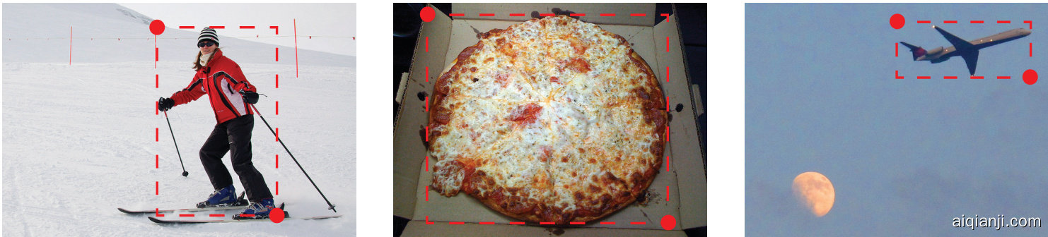
Fig. 2 Often there is no local evidence to determine the location of a bounding box corner. We address this issue by proposing a new type of pooling layer.
图 2: 通常没有局部证据可用于确定边界框角点的位置。我们通过提出一种新型池化层来解决这个问题。
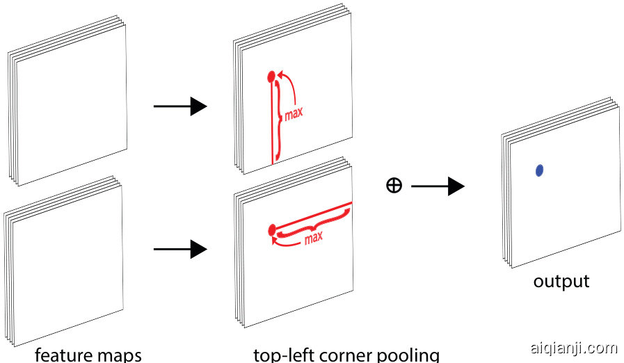
Fig. 3 Corner pooling: for each channel, we take the maximum values (red dots) in two directions (red lines), each from a separate feature map, and add the two maximums together (blue dot).
图 3: 角点池化 (Corner pooling) : 对于每个通道, 我们从两个方向 (红线) 的特征图中分别提取最大值 (红点), 并将两个最大值相加 (蓝点)。
2.2 One-stage object detectors
2.2 单阶段目标检测器
On the other hand, YOLO (Redmon et al., 2016) and SSD (Liu et al., 2016) have popularized the one-stage approach, which removes the RoI pooling step and detects objects in a single network. One-stage detectors are usually more computationally efficient than twostage detectors while maintaining competitive performance on different challenging benchmarks.
另一方面,YOLO (Redmon et al., 2016) 和 SSD (Liu et al., 2016) 普及了单阶段方法,该方法移除了 RoI 池化步骤,直接在单一网络中检测物体。单阶段检测器通常比两阶段检测器计算效率更高,同时在不同挑战性基准测试中保持具有竞争力的性能。
SSD places anchor boxes densely over feature maps from multiple scales, directly classifies and refines each anchor box. YOLO predicts bounding box coordinates directly from an image, and is later improved in YOLO9000 ( mon and Farhadi, 2016) by switching to anchor boxes. DSSD (Fu et al., 2017) and RON (Kong et al., 2017) adopt networks similar to the hourglass network (Newell et al., 2016), enabling them to combine low-level and high-level features via skip connections to predict bounding boxes more accurately. However, these one-stage detectors are still outperformed by the two-stage detectors until the introduction of RetinaNet (Lin et al., 2017). In (Lin et al., 2017), the authors suggest that the dense anchor boxes create a huge imbalance between positive and negative anchor boxes during training. This imbalance causes the training to be inefficient and hence the performance to be suboptimal. They propose a new loss, Focal Loss, to dynamically adjust the weights of each anchor box and show that their onestage detector can outperform the two-stage detectors. RefineDet (Zhang et al., 2017) proposes to filter the an
SSD在多个尺度的特征图上密集放置锚框(anchor boxes),直接对每个锚框进行分类和精修。YOLO直接从图像预测边界框坐标,后在YOLO9000 (Redmon和Farhadi, 2016)中改用锚框进行改进。DSSD (Fu等人, 2017)和RON (Kong等人, 2017)采用类似沙漏网络(hourglass network) (Newell等人, 2016)的结构,通过跳跃连接(skip connections)结合低级和高级特征来更准确地预测边界框。但在RetinaNet (Lin等人, 2017)提出前,这些单阶段检测器的性能仍落后于两阶段检测器。Lin等人(2017)指出,密集锚框会导致训练时正负锚框数量严重失衡,这种失衡导致训练效率低下,从而使性能欠佳。他们提出Focal Loss动态调整每个锚框的权重,证明其单阶段检测器可以超越两阶段检测器。RefineDet (Zhang等人, 2017)提出通过...
chor boxes to reduce the number of negative boxes, and to coarsely adjust the anchor boxes.
通过调整锚框(anchor boxes)以减少负样本框数量,并粗略校准锚框位置。
DeNet (Tychsen-Smith and Petersson, 2017a) is a two-stage detector which generates RoIs without using anchor boxes. It first determines how likely each location belongs to either the top-left, top-right, bottom- left or bottom-right corner of a bounding box. It then generates RoIs by enumerating all possible corner combinations, and follows the standard two-stage approach to classify each RoI. Our approach is very different from DeNet. First, DeNet does not identify if two corners are from the same objects and relies on a sub-detection network to reject poor RoIs. In contrast, our approach is a one-stage approach which detects and groups the corners using a single ConvNet. Second, DeNet selects features at manually determined locations relative to a region for classification, while our approach does not require any feature selection step. Third, we introduce corner pooling, a novel type of layer to enhance corner detection.
DeNet (Tychsen-Smith和Petersson, 2017a) 是一种不使用锚框(anchor boxes)生成候选区域(RoIs)的两阶段检测器。它首先判断每个位置属于边界框左上、右上、左下或右下角的概率,然后通过枚举所有可能的角点组合生成RoIs,并采用标准的两阶段方法对每个RoI进行分类。我们的方法与DeNet存在显著差异:首先,DeNet无法判断两个角点是否属于同一物体,需要依赖子检测网络剔除低质量RoIs;而我们的单阶段方法通过单一卷积网络即可完成角点检测与分组。其次,DeNet需要根据区域位置手动选择分类特征,而我们的方法无需特征选择步骤。第三,我们创新性地引入了角点池化(corner pooling)层来增强角点检测能力。
Point Linking Network (PLN) (Wang et al., 2017) is an one-stage detector without anchor boxes. It first predicts the locations of the four corners and the center of a bounding box. Then, at each corner location, it predicts how likely each pixel location in the image is the center. Similarly, at the center location, it predicts how likely each pixel location belongs to either the top-left, top-right, bottom-left or bottom-right corner. It combines the predictions from each corner and center pair to generate a bounding box. Finally, it merges the four bounding boxes to give a bounding box. CornerNet is very different from PLN. First, CornerNet groups the corners by predicting embedding vectors, while PLN groups the corner and center by predicting pixel locations. Second, CornerNet uses corner pooling to better localize the corners.
点连接网络 (PLN) (Wang et al., 2017) 是一种无需锚框的单阶段检测器。它首先预测边界框的四个角点和中心点位置,然后在每个角点位置预测图像中每个像素位置作为中心点的概率。类似地,在中心点位置预测每个像素位置属于左上、右上、左下或右下角点的概率。通过组合每个角点-中心点对的预测结果生成边界框,最终合并四个边界框得到最终检测框。CornerNet 与 PLN 存在显著差异:首先,CornerNet 通过预测嵌入向量来分组角点,而 PLN 通过预测像素位置来关联角点和中心点;其次,CornerNet 采用角点池化 (corner pooling) 来精确定位角点。
Our approach is inspired by Newell et al. (2017) on Associative Embedding in the context of multi-person pose estimation. Newell et al. propose an approach that detects and groups human joints in a single network. In their approach each detected human joint has an embedding vector. The joints are grouped based on the distances between their embeddings. To the best of our knowledge, we are the first to formulate the task of object detection as a task of detecting and grouping corners with embeddings. Another novelty of ours is the corner pooling layers that help better localize the corners. We also significantly modify the hourglass architecture and add our novel variant of focal loss (Lin et al., 2017) to help better train the network.
我们的方法受到Newell等人(2017)在多人体姿态估计中提出的关联嵌入(Associative Embedding)启发。Newell等人提出了一种在单一网络中检测并分组人体关节的方法。在他们的方法中,每个检测到的人体关节都有一个嵌入向量,关节根据其嵌入向量之间的距离进行分组。据我们所知,我们是首个将目标检测任务表述为"用嵌入向量检测并分组角点"的研究。我们的另一个创新是提出了帮助精确定位角点的角点池化层(corner pooling layers)。我们还显著改进了沙漏网络架构(hourglass architecture),并加入了我们改进的焦点损失(focal loss)(Lin等人,2017)变体来优化网络训练。
3 CornerNet
3 CornerNet
3.1 Overview
3.1 概述
In CornerNet, we detect an object as a pair of keypoints— the top-left corner and bottom-right corner of the bounding box. A convolutional network predicts two sets of heatmaps to represent the locations of corners of different object categories, one set for the top-left corners and the other for the bottom-right corners. The network also predicts an embedding vector for each detected corner (Newell et al., 2017) such that the distance between the embeddings of two corners from the same object is small. To produce tighter bounding boxes, the network also predicts offsets to slightly adjust the locations of the corners. With the predicted heatmaps, embeddings and offsets, we apply a simple post-processing algorithm to obtain the final bounding boxes.
在CornerNet中,我们将目标检测视为一对关键点——边界框的左上角与右下角。卷积网络通过预测两组热力图来表示不同目标类别的角点位置:一组对应左上角,另一组对应右下角。该网络还会为每个检测到的角点预测一个嵌入向量 (Newell et al., 2017) ,使得来自同一目标的两个角点嵌入向量间距较小。为生成更精准的边界框,网络还预测偏移量以微调角点位置。基于预测的热力图、嵌入向量及偏移量,我们采用简单的后处理算法来获得最终边界框。
Fig. 4 provides an overview of CornerNet. We use the hourglass network (Newell et al., 2016) as the backbone network of CornerNet. The hourglass network is followed by two prediction modules. One module is for the top-left corners, while the other one is for the bottomright corners. Each module has its own corner pooling module to pool features from the hourglass network before predicting the heatmaps, embeddings and offsets. Unlike many other object detectors, we do not use features from different scales to detect objects of different sizes. We only apply both modules to the output of the hourglass network.
图 4: CornerNet 整体架构。我们采用 hourglass 网络 (Newell et al., 2016) 作为主干网络,其后连接两个预测模块:一个用于检测左上角点,另一个用于检测右下角点。每个模块均配备独立的角点池化层 (corner pooling),用于在预测热力图 (heatmaps)、嵌入向量 (embeddings) 和偏移量 (offsets) 之前对 hourglass 网络的特征进行池化处理。与多数目标检测器不同,本方法不采用多尺度特征来检测不同尺寸目标,而是将两个模块直接应用于 hourglass 网络的输出层。
3.2 Detecting Corners
3.2 角点检测
We predict two sets of heatmaps, one for top-left corners and one for bottom-right corners. Each set of heatmaps has $C$ channels, where $C$ is the number of categories, and is of size $H\times W$ . There is no background channel. Each channel is a binary mask indicating the locations of the corners for a class.
我们预测两组热图,一组对应左上角,另一组对应右下角。每组热图包含 $C$ 个通道($C$ 为类别数量),尺寸为 $H\times W$,不设背景通道。每个通道都是表示某类别角点位置的二值掩码。
For each corner, there is one ground-truth positive location, and all other locations are negative. During training, instead of equally penalizing negative locations, we reduce the penalty given to negative locations within a radius of the positive location. This is because a pair of false corner detections, if they are close to their respective ground truth locations, can still produce a box that sufficiently overlaps the ground-truth box (Fig. 5). We determine the radius by the size of an object by ensuring that a pair of points within the radius would generate a bounding box with at least $t$ IoU with the ground-truth annotation (we set $t$ to 0.3 in all experiments). Given the radius, the amount of penalty reduction is given by an un normalized 2D Gaussian, $e^{-\frac{x^{2}+y^{2}}{2\sigma^{2}}}$ whose center is at the positive location and whose $\sigma$ is $1/3$ of the radius.
对于每个角点,有一个真实标注的正样本位置,其余位置均为负样本。在训练过程中,我们并非对所有负样本位置施加同等惩罚,而是降低对正样本位置半径范围内负样本的惩罚力度。这是因为即使一对角点检测错误,只要它们距离各自真实位置足够近,仍能生成与真实标注框有足够交并比(IoU)的预测框(图5)。我们根据目标尺寸确定半径范围,确保半径内任意两点生成的边界框与真实标注的IoU至少达到$t$(所有实验设为0.3)。给定半径后,惩罚衰减量由非归一化的二维高斯函数$e^{-\frac{x^{2}+y^{2}}{2\sigma^{2}}}$决定,其中心位于正样本位置,$\sigma$取半径的$1/3$。
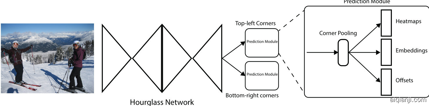
Fig. 4 Overview of CornerNet. The backbone network is followed by two prediction modules, one for the top-left corners and the other for the bottom-right corners. Using the predictions from both modules, we locate and group the corners.
图 4: CornerNet 整体架构。主干网络后接两个预测模块,分别用于预测左上角点和右下角点。通过整合两个模块的预测结果,我们实现角点定位与配对。

Fig. 5 “Ground-truth” heatmaps for training. Boxes (green dotted rectangles) whose corners are within the radii of the positive locations (orange circles) still have large overlaps with the ground-truth annotations (red solid rectangles).
图 5: 训练用的"真实值"热力图。角点位于正样本位置(橙色圆圈)半径范围内的框(绿色虚线矩形)仍与真实标注(红色实线矩形)存在较大重叠区域。
Let $p_{c i j}$ be the score at location $(i,j)$ for class $c$ in the predicted heatmaps, and let $y_{c i j}$ be the “groundtruth” heatmap augmented with the un normalized Gaussians. We design a variant of focal loss (Lin et al., 2017):
设 $p_{c i j}$ 为预测热力图中类别 $c$ 在位置 $(i,j)$ 处的得分,$y_{c i j}$ 为用未归一化高斯分布增强的"真实"热力图。我们设计了一种焦点损失 (focal loss) [20] 的变体:
$$
L_{det} = \frac{1}{N} \sum_{c = 1}^{C} \sum_{i = 1}^{H} \sum_{j = 1}^{W}
\begin{cases}
(1 - p_{cij})^{\alpha} \log(p_{cij}) & \text{if } y_{cij} = 1 \\
(1 - y_{cij})^{\alpha} (p_{cij})^{\alpha} \log(1 - p_{cij}) & \text{otherwise}
\end{cases}
$$
$$
L_{det} = \frac{1}{N} \sum_{c = 1}^{C} \sum_{i = 1}^{H} \sum_{j = 1}^{W}
\begin{cases}
(1 - p_{cij})^{\alpha} \log(p_{cij}) & \text{if } y_{cij} = 1 \\
(1 - y_{cij})^{\alpha} (p_{cij})^{\alpha} \log(1 - p_{cij}) & \text{otherwise}
\end{cases}
$$
where $N$ is the number of objects in an image, and $\alpha$ and $\beta$ are the hyper-parameters which control the contribution of each point (we set $\alpha$ to 2 and $\beta$ to 4 in all experiments). With the Gaussian bumps encoded in $y_{c i j}$ , the $(1-y_{c i j})$ term reduces the penalty around the ground truth locations.
其中 $N$ 是图像中的物体数量,$\alpha$ 和 $\beta$ 是控制各点贡献的超参数 (我们在所有实验中设置 $\alpha$ 为 2,$\beta$ 为 4)。通过 $y_{cij}$ 编码的高斯凸起,$(1-y_{cij})$ 项会减少真实位置周围的惩罚。
Many networks (He et al., 2016; Newell et al., 2016) involve down sampling layers to gather global information and to reduce memory usage. When they are applied to an image fully convolution ally, the size of the output is usually smaller than the image. Hence, a location $(x,y)$ in the image is mapped to the location $\left(\left\lfloor{\frac{x}{n}}\right\rfloor,\left\lfloor{\frac{y}{n}}\right\rfloor\right)$ in the heatmaps, where $n$ is the downsampling factor. When we remap the locations from the heatmaps to the input image, some precision may be lost, which can greatly affect the IoU of small bounding boxes with their ground truths. To address this issue we predict location offsets to slightly adjust the corner locations before remapping them to the input resolution.
许多网络(He等人,2016;Newell等人,2016)采用下采样层来收集全局信息并减少内存使用。当它们以全卷积方式应用于图像时,输出尺寸通常小于原图。因此,图像中的位置$(x,y)$会被映射到热图中的位置$\left(\left\lfloor{\frac{x}{n}}\right\rfloor,\left\lfloor{\frac{y}{n}}\right\rfloor\right)$,其中$n$为下采样因子。当我们将位置从热图重新映射回输入图像时,可能会损失部分精度,这会极大影响小边界框与其真实标注之间的交并比(IoU)。为解决该问题,我们预测位置偏移量,在将角点位置重新映射到输入分辨率前进行微调。
$$
\boldsymbol{o}_ k=\left(\frac{x_{k}}{n}-\left\lfloor\frac{x_{k}}{n}\right\rfloor,\frac{y_{k}}{n}-\left\lfloor\frac{y_{k}}{n}\right\rfloor\right)
$$
$$
\boldsymbol{o}_ k=\left(\frac{x_{k}}{n}-\left\lfloor\frac{x_{k}}{n}\right\rfloor,\frac{y_{k}}{n}-\left\lfloor\frac{y_{k}}{n}\right\rfloor\right)
$$
where $o_{k}$ is the offset, $x_{k}$ and $y_{k}$ are the x and y coordinate for corner $k$ . In particular, we predict one set of offsets shared by the top-left corners of all categories, and another set shared by the bottom-right corners. For training, we apply the smooth L1 Loss (Girshick, 2015) at ground-truth corner locations:
其中 $o_{k}$ 是偏移量,$x_{k}$ 和 $y_{k}$ 是角点 $k$ 的 x 和 y 坐标。具体而言,我们预测一组由所有类别的左上角共享的偏移量,以及另一组由右下角共享的偏移量。在训练时,我们在真实角点位置应用平滑 L1 损失函数 (Girshick, 2015):
$$
L_{o f f}=\frac{1}{N}\sum_{k=1}^{N}\mathrm{SmoothL1Loss}\left(\boldsymbol{o}_ {k},\hat{\boldsymbol{\sigma}}_{k}\right)
$$
$$
L_{o f f}=\frac{1}{N}\sum_{k=1}^{N}\mathrm{SmoothL1Loss}\left(\boldsymbol{o}_ {k},\hat{\boldsymbol{\sigma}}_{k}\right)
$$
3.3 Grouping Corners
3.3 角点分组
Multiple objects may appear in an image, and thus multiple top-left and bottom-right corners may be detected. We need to determine if a pair of the top-left corner and bottom-right corner is from the same bounding box. Our approach is inspired by the Associative Embedding method proposed by Newell et al. (2017) for the task of multi-person pose estimation. Newell et al. detect all human joints and generate an embedding for each detected joint. They group the joints based on the distances between the embeddings.
图像中可能出现多个物体,因此可能检测到多个左上角和右下角。我们需要判断左上角和右下角是否来自同一个边界框。我们的方法受到Newell等人(2017)为多人姿态估计任务提出的关联嵌入(Associative Embedding)方法的启发。Newell等人检测所有人体的关节并为每个检测到的关节生成一个嵌入表示,然后根据嵌入之间的距离对关节进行分组。
The idea of associative embedding is also applicable to our task. The network predicts an embedding vector for each detected corner such that if a top-left corner and a bottom-right corner belong to the same bounding box, the distance between their embeddings should be small. We can then group the corners based on the distances between the embeddings of the top-left and bottom-right corners. The actual values of the embed- dings are unimportant. Only the distances between the embeddings are used to group the corners.
关联嵌入 (associative embedding) 的思想同样适用于我们的任务。网络为每个检测到的角点预测一个嵌入向量,若某个左上角点与右下角点属于同一个边界框,则它们的嵌入向量距离应当较小。随后我们可以根据左上角点与右下角点嵌入向量之间的距离对角点进行分组。嵌入向量的实际数值并不重要,仅通过嵌入向量之间的距离来实现角点分组。
We follow Newell et al. (2017) and use embeddings of 1 dimension. Let $e_{t_{k}}$ be the embedding for the top-left corner of object $k$ and for the bottom-right corner. $e_{b_{k}}$ As in Newell and Deng (2017), we use the “pull” loss to train the network to group the corners and the “push” loss to separate the corners:
我们遵循 Newell 等人 (2017) 的方法,使用 1 维嵌入。设 $e_{t_{k}}$ 为物体 $k$ 左上角的嵌入,$e_{b_{k}}$ 为右下角的嵌入。如 Newell 和 Deng (2017) 所述,我们使用"pull"损失训练网络以聚集角点,使用"push"损失以分离角点:
$$
L_{p u l l}=\frac{1}{N}\sum_{k=1}^{N}\left[\left(e_{t_{k}}-e_{k}\right)^{2}+\left(e_{b_{k}}-e_{k}\right)^{2}\right],
$$
$$
L_{p u l l}=\frac{1}{N}\sum_{k=1}^{N}\left[\left(e_{t_{k}}-e_{k}\right)^{2}+\left(e_{b_{k}}-e_{k}\right)^{2}\right],
$$
$$
L_{p u s h}=\frac{1}{N(N-1)}\sum_{k=1}^{N}\sum_{j=1\atop j\neq k}^{N}\operatorname*{max}\left(0,\varDelta-|e_{k}-e_{j}|\right),
$$
$$
L_{p u s h}=\frac{1}{N(N-1)}\sum_{k=1}^{N}\sum_{j=1\atop j\neq k}^{N}\operatorname*{max}\left(0,\varDelta-|e_{k}-e_{j}|\right),
$$
where $e_{k}$ is the average of $e_{t_{k}}$ and $e_{b_{k}}$ and we set $\varDelta$ to be 1 in all our experiments. Similar to the offset loss, we only apply the losses at the ground-truth corner location.
其中 $e_{k}$ 是 $e_{t_{k}}$ 和 $e_{b_{k}}$ 的平均值,我们在所有实验中设置 $\varDelta$ 为1。与偏移损失类似,我们仅在真实角点位置应用这些损失。
3.4 Corner Pooling
3.4 角点池化 (Corner Pooling)
As shown in Fig. 2, there is often no local visual evidence for the presence of corners. To determine if a pixel is a top-left corner, we need to look horizontally towards the right for the topmost boundary of an object and vertically towards the bottom for the leftmost boundary. We thus propose corner pooling to better localize the corners by encoding explicit prior knowledge.
如图 2 所示,通常不存在局部视觉证据来判定角点的存在。要判断某个像素是否为左上角点,我们需要水平向右寻找物体的最上边界,并垂直向下寻找最左边界。因此,我们提出角点池化 (corner pooling) 方法,通过编码显式先验知识来更准确定位角点。
Suppose we want to determine if a pixel at location $(i,j)$ is a top-left corner. Let $f_{t}$ and $f_{l}$ be the feature maps that are the inputs to the top-left corner pooling layer, and let $f_{t_{i j}}$ and $f_{l_{i j}}$ be the vectors at location $(i,j)$ in $f_{t}$ and $f_{l}$ respectively. With $H\times W$ feature maps, the corner pooling layer first max-pools all feature vectors between $(i,j)$ and $(i,H)$ in $f_{t}$ to a feature vector $t_{i j}$ , and max-pools all feature vectors between $(i,j)$ and $(W,j)$ in $f_{l}$ to a feature vector $l_{i j}$ . Finally, it adds $t_{i j}$ and $l_{i j}$ together. This computation can be expressed by the following equations:
假设我们需要判断位置 $(i,j)$ 的像素是否为左上角。设 $f_{t}$ 和 $f_{l}$ 是输入到左上角池化层的特征图,$f_{t_{i j}}$ 和 $f_{l_{i j}}$ 分别表示 $f_{t}$ 和 $f_{l}$ 在位置 $(i,j)$ 的向量。对于 $H\times W$ 的特征图,角点池化层首先对 $f_{t}$ 中 $(i,j)$ 到 $(i,H)$ 之间的所有特征向量进行最大池化得到 $t_{i j}$,并对 $f_{l}$ 中 $(i,j)$ 到 $(W,j)$ 之间的所有特征向量进行最大池化得到 $l_{i j}$。最终将 $t_{i j}$ 和 $l_{i j}$ 相加。该计算过程可通过以下公式表示:
$$
t_{ij} =
\begin{cases}
\max(f_{t_{ij}}, t_{(i + 1)j}) & \text{if } i < H \\
f_{t_{Hj}} & \text{otherwise}
\end{cases}
$$
$$
t_{ij} =
\begin{cases}
\max(f_{t_{ij}}, t_{(i + 1)j}) & \text{if } i < H \\
f_{t_{Hj}} & \text{otherwise}
\end{cases}
$$
$$
l_{ij} =
\begin{cases}
\max(f_{l_{ij}}, l_{i(j + 1)}) & \text{if } j < W \\
f_{l_{iW}} & \text{otherwise}
\end{cases}
$$
$$
l_{ij} =
\begin{cases}
\max(f_{l_{ij}}, l_{i(j + 1)}) & \text{if } j < W \\
f_{l_{iW}} & \text{otherwise}
\end{cases}
$$
where we apply an element wise max operation. Both $t_{i j}$ and $\mathit{l}_{i j}$ can be computed efficiently by dynamic programming as shown Fig. 8.
我们对元素进行逐项取最大值操作。$t_{i j}$ 和 $\mathit{l}_{i j}$ 都可以通过动态编程高效计算,如图 8 所示。
We define bottom-right corner pooling layer in a similar way. It max-pools all feature vectors between $(0,j)$ and $(i,j)$ , and all feature vectors between $(i,0)$ and $(i,j)$ before adding the pooled results. The corner pooling layers are used in the prediction modules to predict heatmaps, embeddings and offsets.
我们以类似的方式定义右下角池化层。它会对 $(0,j)$ 到 $(i,j)$ 之间以及 $(i,0)$ 到 $(i,j)$ 之间的所有特征向量进行最大池化,然后将池化结果相加。角池化层被用于预测模块中来预测热力图、嵌入向量和偏移量。
The architecture of the prediction module is shown in Fig. 7. The first part of the module is a modified version of the residual block (He et al., 2016). In this modified residual block, we replace the first $3\times3$ convolution module with a corner pooling module, which first processes the features from the backbone network by two $3\times3$ convolution modules 1 with 128 channels and then applies a corner pooling layer. Following the design of a residual block, we then feed the pooled features into a $3\times3$ Conv-BN layer with 256 channels and add back the projection shortcut. The modified residual block is followed by a $3\times3$ convolution module with 256 channels, and 3 Conv-ReLU-Conv layers to produce the heatmaps, embeddings and offsets.
预测模块的架构如图7所示。该模块的第一部分是改进版的残差块 (He et al., 2016)。在这个改进的残差块中,我们将第一个$3\times3$卷积模块替换为角点池化模块,该模块首先通过两个128通道的$3\times3$卷积模块1处理来自主干网络的特征,然后应用角点池化层。遵循残差块的设计,我们将池化后的特征输入到256通道的$3\times3$ Conv-BN层,并添加投影捷径连接。改进后的残差块后面接一个256通道的$3\times3$卷积模块,以及3个Conv-ReLU-Conv层来生成热图、嵌入向量和偏移量。
3.5 Hourglass Network
3.5 Hourglass Network
CornerNet uses the hourglass network (Newell et al., 2016) as its backbone network. The hourglass network was first introduced for the human pose estimation task. It is a fully convolutional neural network that consists of one or more hourglass modules. An hourglass module first down samples the input features by a series of convolution and max pooling layers. It then upsamples the features back to the original resolution by a series of upsampling and convolution layers. Since details are lost in the max pooling layers, skip layers are added to bring back the details to the upsampled features. The hourglass module captures both global and local features in a single unified structure. When multiple hourglass modules are stacked in the network, the hourglass modules can reprocess the features to capture higher-level of information. These properties make the hourglass network an ideal choice for object detection as well. In fact, many current detectors (Shri vast ava et al., 2016; Fu et al., 2017; Lin et al., 2016; Kong et al., 2017) already adopted networks similar to the hourglass network.
CornerNet采用hourglass网络(Newell等人,2016)作为其主干网络。该网络最初是为人体姿态估计任务提出的,是一种完全卷积神经网络,包含一个或多个hourglass模块。hourglass模块首先通过一系列卷积和最大池化层对输入特征进行下采样,然后通过上采样和卷积层将特征恢复至原始分辨率。由于最大池化层会丢失细节信息,因此添加跳跃连接(skip layers)将细节信息带回上采样特征。hourglass模块在单一统一结构中同时捕获全局和局部特征。当网络堆叠多个hourglass模块时,这些模块能对特征进行再处理以捕获更高层次的信息。这些特性使得hourglass网络同样成为目标检测的理想选择。事实上,许多现有检测器(Shri vast ava等人,2016;Fu等人,2017;Lin等人,2016;Kong等人,2017)已采用类似hourglass的网络结构。
Our hourglass network consists of two hourglasses, and we make some modifications to the architecture of the hourglass module. Instead of using max pooling, we simply use stride 2 to reduce feature resolution. We reduce feature resolutions 5 times and in- crease the number of feature channels along the way (256, 384, 384, 384, 512). When we upsample the features, we apply 2 residual modules followed by a nearest neighbor upsampling. Every skip connection also consists of 2 residual modules. There are 4 residual modules with 512 channels in the middle of an hourglass module. Before the hourglass modules, we reduce the image resolution by 4 times using a $7\times7$ convolution module with stride 2 and 128 channels followed by a residual block (He et al., 2016) with stride 2 and 256 channels.
我们的沙漏网络由两个沙漏模块组成,并对沙漏模块的架构进行了一些修改。我们不再使用最大池化,而是简单地使用步长为2的卷积来降低特征分辨率。我们将特征分辨率降低5次,并在此过程中逐步增加特征通道数(256、384、384、384、512)。在上采样特征时,我们应用2个残差模块,然后进行最近邻上采样。每个跳跃连接也由2个残差模块组成。在沙漏模块中间有4个512通道的残差模块。在沙漏模块之前,我们使用步长为2的$7\times7$卷积模块(128通道)和步长为2的残差块(256通道)[He et al., 2016]将图像分辨率降低4倍。

Fig. 6 The top-left corner pooling layer can be implemented very efficiently. We scan from right to left for the horizontal max-pooling and from bottom to top for the vertical max-pooling. We then add two max-pooled feature maps.
图 6: 左上角池化层可实现高效运算。水平方向采用从右至左扫描的最大池化,垂直方向采用从下至上扫描的最大池化,最后将两个最大池化特征图相加。

Fig. 7 The prediction module starts with a modified residual block, in which we replace the first convolution module with our corner pooling module. The modified residual block is then followed by a convolution module. We have multiple branches for predicting the heatmaps, embeddings and offsets.
图 7: 预测模块以改进的残差块 (residual block) 开始,其中我们将第一个卷积模块替换为角点池化 (corner pooling) 模块。改进的残差块后接一个卷积模块。我们通过多个分支来预测热图 (heatmaps)、嵌入向量 (embeddings) 和偏移量 (offsets)。
Following (Newell et al., 2016), we also add intermediate supervision in training. However, we do not add back the intermediate predictions to the network as we find that this hurts the performance of the network. We apply a $1\times1$ Conv-BN module to both the input and output of the first hourglass module. We then merge them by element-wise addition followed by a ReLU and a residual block with 256 channels, which is then used as the input to the second hourglass module. The depth of the hourglass network is 104. Unlike many other stateof-the-art detectors, we only use the features from the last layer of the whole network to make predictions.
遵循 (Newell et al., 2016) 的方法,我们在训练中也加入了中间监督。不过,我们发现将中间预测重新加入网络会损害其性能,因此没有这样做。我们对第一个沙漏模块的输入和输出都应用了 $1\times1$ 的 Conv-BN 模块,然后通过逐元素相加进行融合,接着经过一个 ReLU 和一个 256 通道的残差块,最后将其作为第二个沙漏模块的输入。该沙漏网络的深度为 104。与许多其他先进检测器不同,我们仅使用整个网络最后一层的特征进行预测。
4 Experiments
4 实验
4.1 Training Details
4.1 训练细节
We implement CornerNet in PyTorch (Paszke et al., 2017). The network is randomly initialized under the default setting of PyTorch with no pre training on any external dataset. As we apply focal loss, we follow (Lin et al., 2017) to set the biases in the convolution layers that predict the corner heatmaps. During training, we set the input resolution of the network to $511\times511$ , which leads to an output resolution of $128\times128$ . To reduce over fitting, we adopt standard data augmentation techniques including random horizontal flipping, random scaling, random cropping and random color jittering, which includes adjusting the brightness, saturation and contrast of an image. Finally, we apply PCA (Krizhevsky et al., 2012) to the input image.
我们在PyTorch (Paszke et al., 2017) 中实现了CornerNet。网络在PyTorch默认设置下随机初始化,未使用任何外部数据集进行预训练。由于采用了焦点损失 (focal loss),我们遵循 (Lin et al., 2017) 的方法设置预测角点热图的卷积层偏置。训练过程中,我们将网络输入分辨率设为 $511\times511$,输出分辨率为 $128\times128$。为减少过拟合,我们采用了标准数据增强技术,包括随机水平翻转、随机缩放、随机裁剪和随机色彩抖动(含图像亮度、饱和度和对比度调整)。最后对输入图像应用了PCA (Krizhevsky et al., 2012)。
We use Adam (Kingma and Ba, 2014) to optimize the full training loss:
我们使用 Adam (Kingma and Ba, 2014) 优化完整训练损失:
$$
L=L_{d e t}+\alpha L_{p u l l}+\beta L_{p u s h}+\gamma L_{o f f}
$$
$$
L=L_{d e t}+\alpha L_{p u l l}+\beta L_{p u s h}+\gamma L_{o f f}
$$
where $\alpha$ , $\beta$ and $\gamma$ are the weights for the pull, push and offset loss respectively. We set both $\alpha$ and $\beta$ to 0.1 and $\gamma$ to 1. We find that 1 or larger values of $\alpha$ and $\beta$ lead to poor performance. We use a batch size of 49 and train the network on 10 Titan X (PASCAL) GPUs (4 images on the master GPU, 5 images per GPU for the rest of the GPUs). To conserve GPU resources, in our ablation experiments, we train the networks for 250k iterations with a learning rate of $2.5\times10^{-4}$ . When we compare our results with other detectors, we train the networks for an extra 250k iterations and reduce the learning rate to $2.5\times10^{-5}$ for the last 50k iterations.
其中 $\alpha$ 、 $\beta$ 和 $\gamma$ 分别是拉力、推力和偏移损失的权重。我们将 $\alpha$ 和 $\beta$ 设为 0.1, $\gamma$ 设为 1。我们发现当 $\alpha$ 和 $\beta$ 取 1 或更大值时性能会下降。我们使用批量大小为 49,并在 10 块 Titan X (PASCAL) GPU 上训练网络 (主 GPU 处理 4 张图像,其余 GPU 每块处理 5 张图像)。为节省 GPU 资源,在消融实验中,我们以 $2.5\times10^{-4}$ 的学习率训练网络 25 万次迭代。当与其他检测器对比结果时,我们会额外训练 25 万次迭代,并在最后 5 万次迭代时将学习率降至 $2.5\times10^{-5}$。
Table 1 Ablation on corner pooling on MS COCO validation.
| AP | AP50 | AP75 | APs APm | APl | |
| w/o corner p pooling | 36.5 | 52.0 | 38.8 | 17.5 38.9 | 49.4 |
| w/ corner pooling | 38.4 | 53.8 | 40.9 | 18.6 40.5 | 51.8 |
| improvement | +2.0 | +2.1 | +2.1 | +1.1 +2.4 | +3.6 |
表 1: MS COCO验证集上角点池化 (corner pooling) 的消融实验
| AP | AP50 | AP75 | APs APm | APl | |
|---|---|---|---|---|---|
| 不使用角点池化 | 36.5 | 52.0 | 38.8 | 17.5 38.9 | 49.4 |
| 使用角点池化 | 38.4 | 53.8 | 40.9 | 18.6 40.5 | 51.8 |
| 提升幅度 | +2.0 | +2.1 | +2.1 | +1.1 +2.4 | +3.6 |
Table 2 Reducing the penalty given to the negative locations near positive locations helps significantly improve the performance of the network
| AP | AP50 | AP75 | APs | APm | APl | |
| w/o reducing penalty | 32.9 | 49.1 | 34.8 | 19.0 | 37.0 | 40.7 |
| fixed 1 radius | 35.6 | 52.5 | 37.7 | 18.7 | 38.5 | 46.0 |
| object-dependent radius | 38.4 | 53.8 | 40.9 | 18.6 | 40.5 | 51.8 |
表 2: 降低正样本位置附近负样本位置的惩罚能显著提升网络性能
| AP | AP50 | AP75 | APs | APm | APl | |
|---|---|---|---|---|---|---|
| 不降低惩罚 | 32.9 | 49.1 | 34.8 | 19.0 | 37.0 | 40.7 |
| 固定1半径 | 35.6 | 52.5 | 37.7 | 18.7 | 38.5 | 46.0 |
| 目标依赖半径 | 38.4 | 53.8 | 40.9 | 18.6 | 40.5 | 51.8 |
Table 3 Corner pooling consistently improves the network performance on detecting corners in different image quadrants, showing that corner pooling is effective and stable over both small and large areas.
| mAP w/o pooling | mAP w/pooling | improvement | |
| Top-Left Corners | |||
| Iop-LeftQuad. | 66.1 | 69.2 | +3.1 |
| Bottom-Right Quad. | 60.8 | 63.5 | +2.7 |
| Bottom-Right Corners | |||
| Top-Left Quad. | 53.4 | 56.2 | +2.8 |
| Bottom-Right Quad. | 65.0 | 67.6 | +2.6 |
表 3: 角点池化在不同图像象限的角点检测中持续提升网络性能,表明角点池化在小区域和大区域上都具有高效性和稳定性。
| 无池化mAP | 带池化mAP | 提升值 | |
|---|---|---|---|
| 左上角点 | |||
| 左上象限 | 66.1 | 69.2 | +3.1 |
| 右下象限 | 60.8 | 63.5 | +2.7 |
| 右下角点 | |||
| 左上象限 | 53.4 | 56.2 | +2.8 |
| 右下象限 | 65.0 | 67.6 | +2.6 |
zeros before feeding it to CornerNet. Both the original and flipped images are used for testing. We combine the detections from the original and flipped images, and apply soft-nms (Bodla et al., 2017) to suppress redundant detections. Only the top 100 detections are reported. The average inference time is 244ms per image on a Titan X (PASCAL) GPU.
在将图像输入CornerNet之前,我们会在两侧用零填充图像。测试时同时使用原始图像和水平翻转图像。我们将原始图像和翻转图像的检测结果合并,并应用软性非极大值抑制(soft-nms) [Bodla et al., 2017] 来抑制冗余检测。最终仅保留前100个检测结果。在Titan X (PASCAL) GPU上,平均每张图像的推理时间为244毫秒。
4.2 Testing Details
4.2 测试详情
During testing, we use a simple post-processing algorithm to generate bounding boxes from the heatmaps, embeddings and offsets. We first apply non-maximal suppression (NMS) by using a 3 $\times$ 3 max pooling layer on the corner heatmaps. Then we pick the top 100 top-left and top 100 bottom-right corners from the heatmaps. The corner locations are adjusted by the corresponding offsets. We calculate the L1 distances between the embeddings of the top-left and bottom-right corners. Pairs that have distances greater than 0.5 or contain corners from different categories are rejected. The average scores of the top-left and bottom-right corners are used as the detection scores.
在测试阶段,我们采用一种简单的后处理算法从热图、嵌入向量和偏移量生成边界框。首先对角落热图应用3×3最大池化层进行非极大值抑制(NMS),随后从热图中选取置信度最高的100个左上角点和100个右下角点。通过对应偏移量调整角点位置后,计算左上角与右下角嵌入向量的L1距离。距离超过0.5或包含不同类别角点的配对将被剔除,最终以左上角与右下角得分的平均值作为检测置信度。
Instead of resizing an image to a fixed size, we maintain the original resolution of the image and pad it with
我们不调整图像至固定尺寸,而是保持其原始分辨率并通过填充处理
4.3 MS COCO
4.3 MS COCO
We evaluate CornerNet on the very challenging MS COCO dataset (Lin et al., 2014). MS COCO contains 80k images for training, 40k for validation and 20k for testing. All images in the training set and 35k images in the validation set are used for training. The remaining 5k images in validation set are used for hyper-parameter searching and ablation study. All results on the test set are submitted to an external server for evaluation. To provide fair comparisons with other detectors, we report our main results on the test-dev set. MS COCO uses average precisions (APs) at different IoUs and APs for different object sizes as the main evaluation metrics.
我们在极具挑战性的 MS COCO 数据集 (Lin et al., 2014) 上评估 CornerNet。MS COCO 包含 8 万张训练图像、4 万张验证图像和 2 万张测试图像。训练集中的所有图像和验证集中的 3.5 万张图像用于训练,验证集剩余的 5 千张图像用于超参数搜索和消融实验。所有测试集结果均提交至外部服务器进行评估。为与其他检测器进行公平比较,我们报告了在 test-dev 集上的主要结果。MS COCO 采用不同 IoU 阈值下的平均精度 (AP) 以及不同物体尺寸的 AP 作为主要评估指标。

Fig. 8 Qualitative examples showing corner pooling helps better localize the corners.
图 8: 定性示例展示角点池化 (corner pooling) 有助于更精准定位角点。
Table 4 The hourglass network is crucial to the performance of CornerNet.
| AP | AP50 | AP75 | APs | APm | APl | |
| FPN N (w/ ResNet-101) + Corners | 30.2 | 44.1 | 32.0 | 13.3 | 33.3 | 42.7 |
| Hourglass + Anchors | 32.9 | 53.1 | 35.6 | 16.5 | 38.5 | 45.0 |
| Hourglass + Corners | 38.4 | 53.8 | 40.9 | 18.6 | 40.5 | 51.8 |
表 4 沙漏网络对CornerNet性能至关重要
| AP | AP50 | AP75 | APs | APm | APl | |
|---|---|---|---|---|---|---|
| FPN N (w/ ResNet-101) + Corners | 30.2 | 44.1 | 32.0 | 13.3 | 33.3 | 42.7 |
| Hourglass + Anchors | 32.9 | 53.1 | 35.6 | 16.5 | 38.5 | 45.0 |
| Hourglass + Corners | 38.4 | 53.8 | 40.9 | 18.6 | 40.5 | 51.8 |
4.4 Ablation Study
4.4 消融实验
4.4.1 Corner Pooling
4.4.1 角点池化 (Corner Pooling)
Corner pooling is a key component of CornerNet. To understand its contribution to performance, we train another network without corner pooling but with the same number of parameters.
角点池化 (corner pooling) 是CornerNet的关键组件。为了理解其对性能的贡献,我们训练了另一个不使用角点池化但参数数量相同的网络。
Tab. 1 shows that adding corner pooling gives significant improvement: $2.0%$ on AP, $2.1%$ on AP $^{50}$ and $2.1%$ on $\mathrm{AP^{75}}$ . We also see that corner pooling is especially helpful for medium and large objects, improving their APs by $2.4%$ and $3.6%$ respectively. This is expected because the topmost, bottommost, leftmost, rightmost boundaries of medium and large objects are likely to be further away from the corner locations. Fig. 8 shows four qualitative examples with and without corner pooling.
表 1 显示,添加角点池化 (corner pooling) 带来了显著提升:AP 提升 2.0%、AP$^{50}$ 提升 2.1%、$\mathrm{AP^{75}}$ 提升 2.1%。我们还发现角点池化对中型和大型物体特别有效,分别将其 AP 提高了 2.4% 和 3.6%。这是符合预期的,因为中型和大型物体的最顶部、最底部、最左侧和最右侧边界往往距离角点位置较远。图 8 展示了使用和不使用角点池化的四个定性示例。
4.4.2 Stability of Corner Pooling over Larger Area
4.4.2 角点池化在大区域上的稳定性
Corner pooling pools over different sizes of area in different quadrants of an image. For example, the top-left corner pooling pools over larger areas both horizontally and vertically in the upper-left quadrant of an image, compared to the lower-right quadrant. Therefore, the location of a corner may affect the stability of the corner pooling.
角点池化(Corner pooling)在图像的不同象限中对不同大小的区域进行池化。例如,与右下象限相比,左上角点池化在图像的左上象限中水平和垂直方向上对更大的区域进行池化。因此,角点的位置可能会影响角点池化的稳定性。
We evaluate the performance of our network on detecting both the top-left and bottom-right corners in different quadrants of an image. Detecting corners can be seen as a binary classification task i.e. the groundtruth location of a corner is positive, and any location outside of a small radius of the corner is negative. We measure the performance using mAPs over all categories on the MS COCO validation set.
我们在图像不同象限中检测左上角和右下角的性能表现。角点检测可视为二分类任务:以角点真实位置为中心的小半径范围内为正样本,其余区域为负样本。采用MS COCO验证集上所有类别的mAP作为评估指标。
Tab. 3 shows that without corner pooling, the topleft corner mAPs of upper-left and lower-right quadrant are $66.1%$ and $60.8%$ respectively. Top-left corner pooling improves the mAPs by $3.1%$ (to $69.2%$ ) and $2.7%$ (to $63.5%$ ) respectively. Similarly, bottomright corner pooling improves the bottom-right corner mAPs of upper-left quadrant by $2.8%$ (from $53.4%$ to $56.2%$ ), and lower-right quadrant by $2.6%$ (from $65.0%$ to $67.6%$ ). Corner pooling gives similar improvement to corners at different quadrants, show that corner pooling is effective and stable over both small and large areas.
表 3 显示,在没有角点池化 (corner pooling) 的情况下,左上和右下象限的左上角 mAP 分别为 $66.1%$ 和 $60.8%$。左上角池化分别将 mAP 提高了 $3.1%$ (达到 $69.2%$) 和 $2.7%$ (达到 $63.5%$)。类似地,右下角池化将左上象限的右下角 mAP 提高了 $2.8%$ (从 $53.4%$ 提高到 $56.2%$),右下象限提高了 $2.6%$ (从 $65.0%$ 提高到 $67.6%$)。角点池化对不同象限的角点均有相似的提升效果,表明该技术在小区域和大区域上都具有稳定且有效的特性。
4.4.3 Reducing Penalty to Negative Locations
4.4.3 降低负样本位置的惩罚
We reduce the penalty given to negative locations around a positive location, within a radius determined by the size of the object (Sec. 3.2). To understand how this helps train CornerNet, we train one network with no penalty reduction and another network with a fixed radius of 2.5. We compare them with CornerNet on the validation set.
我们降低了对正样本位置周围一定半径内负样本位置的惩罚力度,该半径由物体大小决定(见第3.2节)。为验证该策略对训练CornerNet的效果,我们分别训练了无惩罚缩减的网络和固定半径2.5的网络,并在验证集上与CornerNet进行对比。
Tab. 2 shows that a fixed radius improves AP over the baseline by 2.7%, AP $_ {T I V}$ by $1.5%$ and AP $\mathbf{\nabla}_{\mathbf{\lambda}}l$ by $5.3%$ . Object-dependent radius further improves the AP by
表 2: 固定半径相比基线将AP提升了2.7%,AP$_ {TIV}$提升了$1.5%$,AP$\mathbf{\nabla}_{\mathbf{\lambda}}l$提升了$5.3%$。物体相关半径进一步将AP提高了
Table 5 CornerNet performs much better at high IoUs than other state-of-the-art detectors.
| AP | AP50 | AP60 | AP70 | AP80 | AP90 | |
| RetinaNet (Lin et al., 2017) | 39.8 | 59.5 | 55.6 | 48.2 | 36.4 | 15.1 |
| Cascade R-CNN (Cai and Vasconcelos, 2017) | 38.9 | 57.8 | 53.4 | 46.9 | 35.8 | 15.8 |
| Cascade R-CNN + IoU Net (Jiang et al., 2018) | 41.4 | 59.3 | 55.3 | 49.6 | 39.4 | 19.5 |
| CornerNet | 40.6 | 56.1 | 52.0 | 46.8 | 38.8 | 23.4 |
表 5: CornerNet 在高 IoU 情况下表现远优于其他最先进的检测器。
| AP | AP50 | AP60 | AP70 | AP80 | AP90 | |
|---|---|---|---|---|---|---|
| RetinaNet (Lin et al., 2017) | 39.8 | 59.5 | 55.6 | 48.2 | 36.4 | 15.1 |
| Cascade R-CNN (Cai and Vasconcelos, 2017) | 38.9 | 57.8 | 53.4 | 46.9 | 35.8 | 15.8 |
| Cascade R-CNN + IoU Net (Jiang et al., 2018) | 41.4 | 59.3 | 55.3 | 49.6 | 39.4 | 19.5 |
| CornerNet | 40.6 | 56.1 | 52.0 | 46.8 | 38.8 | 23.4 |
Table 6 Error analysis. We replace the predicted heatmaps and offsets with the ground-truth values. Using the ground-truth heatmaps alone improves the AP from $38.4%$ to $73.1%$ , suggesting that the main bottleneck of CornerNet is detecting corners.
| AP | AP50 | AP75 | APs | APm | APl | ||
| 38.4 | 53.8 | 40.9 | 18.6 | 40.5 | 51.8 | ||
| w/ gt heatmaps | 73.1 | 87.7 | 78.4 | 60.9 | 81.2 | 81.8 | |
| w/ gt heatmaps + offsets | 86.1 | 88.9 | 85.5 | 84.8 | 87.2 | 82.0 | |
表 6: 误差分析。我们将预测的热力图和偏移量替换为真实值。仅使用真实热力图就将AP从 $38.4%$ 提升到 $73.1%$ ,表明CornerNet的主要瓶颈在于检测角点。
| AP | AP50 | AP75 | APs | APm | APl | ||
|---|---|---|---|---|---|---|---|
| 38.4 | 53.8 | 40.9 | 18.6 | 40.5 | 51.8 | ||
| 使用真实热力图 | 73.1 | 87.7 | 78.4 | 60.9 | 81.2 | 81.8 | |
| 使用真实热力图+偏移量 | 86.1 | 88.9 | 85.5 | 84.8 | 87.2 | 82.0 |

Fig. 9 Qualitative example showing errors in predicting corners and embeddings. The first row shows images where CornerNet mistakenly combines boundary evidence from different objects. The second row shows images where CornerNet predicts similar embeddings for corners from different objects.
图 9: 展示角点预测和嵌入向量错误的定性示例。首行图像显示CornerNet误将不同物体的边界证据合并。次行图像显示CornerNet为不同物体的角点预测了相似的嵌入向量。
$2.8%$ , $\mathrm{AP}^{m}$ by $2.0%$ and $\mathrm{AP}^{l}$ by $5.8%$ . In addition, we see that the penalty reduction especially benefits medium and large objects.
$2.8%$,$\mathrm{AP}^{m}$提升$2.0%$,$\mathrm{AP}^{l}$提升$5.8%$。此外,我们发现惩罚机制的优化尤其有利于中型和大型物体。
4.4.4 Hourglass Network
4.4.4 Hourglass Network
CornerNet uses the hourglass network (Newell et al., 2016) as its backbone network. Since the hourglass network is not commonly used in other state-of-the-art detectors, we perform an experiment to study the contribution of the hourglass network in CornerNet. We train a CornerNet in which we replace the hourglass network with FPN (w/ ResNet-101) (Lin et al., 2017), which is more commonly used in state-of-the-art object detectors. We only use the final output of FPN for predictions. Meanwhile, we train an anchor box based detector which uses the hourglass network as its backbone. Each hourglass module predicts anchor boxes at multiple resolutions by using features at multiple scales during upsampling stage. We follow the anchor box design in RetinaNet (Lin et al., 2017) and add intermediate supervisions during training. In both experiments, we initialize the networks from scratch and follow the same training procedure as we train CornerNet (Sec. 4.1).
CornerNet采用hourglass网络(Newell et al., 2016)作为主干网络。由于hourglass网络在其他先进检测器中并不常见,我们进行了一项实验来研究hourglass网络的贡献。我们训练了一个用FPN(带ResNet-101)(Lin et al., 2017)替代hourglass网络的CornerNet版本,FPN在先进目标检测器中更为常用。我们仅使用FPN的最终输出进行预测。同时,我们训练了一个以hourglass网络为主干的基于锚框(anchor box)的检测器。每个hourglass模块在上采样阶段通过多尺度特征来预测多分辨率下的锚框。我们遵循RetinaNet(Lin et al., 2017)中的锚框设计,并在训练过程中添加中间监督。两项实验均从头开始初始化网络,并遵循与训练CornerNet相同的训练流程(第4.1节)。
Tab. 4 shows that CornerNet with hourglass network outperforms CornerNet with FPN by 8.2% AP, and the anchor box based detector with hourglass network by $5.5%$ AP. The results suggest that the choice of the backbone network is important and the hourglass network is crucial to the performance of CornerNet.
表 4 显示,使用 hourglass network 的 CornerNet 比使用 FPN 的 CornerNet 在 AP 上高出 8.2%,比基于 anchor box 的检测器 (使用 hourglass network) 在 AP 上高出 5.5%。结果表明,主干网络的选择很重要,而 hourglass network 对 CornerNet 的性能至关重要。
Table 7 CornerNet versus others on MS COCO test-dev. CornerNet outperforms all one-stage detectors and achieves results competitive to two-stage detectors
| Method | Backbone | AP | AP50 AP75 | AP* | APm | AP | AR | AR10 | AR100 | AR* | ARm | AR | |
| Two-stage detectors | |||||||||||||
| DeNet (Tychsen-Smith and Petersson, 2017a) ResNet-101 | 19.2 | 46.9 | 64.3 | ||||||||||
| CoupleNet (Zhu et al., 2017) | ResNet-101 | 33.8 34.4 | 53.4 54.8 | 36.1 37.2 | 12.3 13.4 | 36.1 38.1 | 50.8 50.8 | 29.6 30.0 | 42.6 45.0 | 43.5 46.4 | 20.7 | 53.1 | 68.5 |
| Faster R-CNN by G-RMI (Huang et al., 2017) | Inception-ResNet-v2 (Szegedy et al., 2017) | 34.7 | 55.5 | 36.7 | 13.5 | 38.1 | 52.0 | ||||||
| 34.9 | 55.7 | 37.4 | 15.6 | 38.7 | 50.9 | 二 | 二 | 二 | 二 | ||||
| Faster R-CNN+++ (He et al., 2016) | ResNet-101 ResNet-101 | 36.2 | 59.1 | 39.0 | 18.2 | 48.2 | 二 | 二 | 二 | 二 | 二 | 二 | |
| Faster R-CNN w/ FPN (Lin et al., 2016) | Inception-ResNet-v2 | 36.8 | 57.7 | 39.2 | 16.2 | 39.0 | 52.1 | ||||||
| Faster R-CNN w/ TDM (Shrivastava et al., 2016) D-FCN (Dai et al., 2017) | Aligned-Inception-ResNet | 37.5 | 58.0 | 19.4 | 39.8 | 52.5 | 31.6 | 49.3 | 51.9 | 28.1 | 56.6 | 71.1 | |
| Regionlets (Xu et al., 2017) | ResNet-101 | 39.3 | 59.8 | 二 | 21.7 | 40.1 43.7 | 50.9 | 二 | 二 | 二 | 二 | 二 | |
| Mask R-CNN (He et al., 2017) | ResNeXt-101 | 39.8 | 62.3 | 43.4 | 22.1 | 43.2 | 51.2 | 二 | 二 | 二 | 二 | 二 | 二 |
| Soft-NMS (Bodla et al., 2017) | Aligned-Inception-ResNet | 40.9 | 62.8 | 23.3 | 43.6 | 53.3 | 二 | ||||||
| LH R-CNN (Li et al., 2017) | ResNet-101 | 41.5 | 25.2 | 45.3 | 53.1 | ||||||||
| Fitness-NMS (Tychsen-Smith and Petersson, 2017b) | ResNet-101 | 41.8 | 60.9 | 44.9 | 21.5 | 45.0 | 57.5 | 二 | 二 | 二 | 二 | ||
| Cascade R-CNN (Cai and Vasconcelos, 2017) | ResNet-101 | 42.8 | 62.1 | 46.3 | 23.7 | 45.5 | 55.2 | 二 | 二 | 二 | 二 | ||
| D-RFCN + SNIP (Singh and Davis, 2017) | DPN-98 (Chen et al., 2017) | 45.7 | 67.3 | 51.1 | 29.3 | 48.8 | 57.1 | 二 | 二 二 | 二 | 二 二 | 二 二 | |
| One-stage detectors | |||||||||||||
| YOLOv2 (Redmon and Farhadi, 2016) DarkNet-19 | |||||||||||||
| DSOD300 (Shen et al., 2017a) | DS/64-192-48-1 | 21.6 29.3 | 44.0 47.3 | 19.2 30.6 | 5.0 9.4 | 22.4 | 35.5 | 20.7 | 31.6 | 9.8 | 36.5 | 54.4 | |
| 31.5 | 47.0 | 27.3 | 40.7 | 43.0 | 16.7 | 47.1 | 65.0 | ||||||
| GRP-DSOD320 (Shen et al., 2017b) | DS/64-192-48-1 | 30.0 | 47.9 | 31.8 | 10.9 | 33.6 | 46.3 | 28.0 | 42.1 | 44.5 | 18.8 | 49.1 | 65.0 |
| SSD513 (Liu et al., 2016) | ResNet-101 | 31.2 | 50.4 | 33.3 | 10.2 | 34.5 | 49.8 | 28.3 | 42.1 | 44.4 | 17.6 | 49.2 | |
| DSSD513 (Fu et al., 2017) | ResNet-101 | 33.2 | 53.3 | 35.2 | 13.0 | 35.4 | 51.1 | 28.9 | 43.5 | 46.2 | 21.8 | 65.8 | |
| RefineDet512 (single scale)(Zhang et al., 2017) | ResNet-101 | 36.4 | 57.5 | 39.5 | 16.6 | 39.9 | 51.4 | 二 | 二 | 二 | 二 | 49.1 | 66.4 |
| RetinaNet800 (Lin et al.,2017) | ResNet-101 | 39.1 | 59.1 | 42.3 | 21.8 | 42.7 | 50.2 | 二 | 二 | 二 | 二 | 二 | 二 二 |
| RefineDet512 (multi scale) (Zhang et al., 2017) | ResNet-101 | 41.8 | 62.9 | 45.7 | 25.6 | 45.1 | 54.1 | 二 | 二 | 二 | 二 | 二 | 二 |
| CornerNet511 (single scale) | Hourglass-104 | 40.6 | 56.4 | 43.2 | 19.1 | 42.8 | 54.3 | 35.3 | 54.7 | 59.4 | 37.4 | 62.4 | 77.2 |
| CornerNet511 (multi scale) | Hourglass-104 | 42.2 | 57.8 | 45.2 | 20.7 | 44.8 | 56.6 | 36.6 | 55.9 | 60.3 | 39.5 | 63.2 | 77.3 |
表 7: CornerNet 与其他方法在 MS COCO test-dev 上的对比。CornerNet 优于所有一阶段检测器,并与二阶段检测器取得相当的结果
| 方法 | 主干网络 | AP | AP50 AP75 | AP* | APm | AP | AR | AR10 | AR100 | AR* | ARm | AR |
|---|---|---|---|---|---|---|---|---|---|---|---|---|
| 二阶段检测器 | ||||||||||||
| DeNet (Tychsen-Smith and Petersson, 2017a) | ResNet-101 | 19.2 | 46.9 | 64.3 | ||||||||
| CoupleNet (Zhu et al., 2017) | ResNet-101 | 33.8 34.4 | 53.4 54.8 | 36.1 37.2 | 12.3 13.4 | 36.1 38.1 | 50.8 50.8 | 29.6 30.0 | 42.6 45.0 | 43.5 46.4 | 20.7 | 53.1 |
| Faster R-CNN by G-RMI (Huang et al., 2017) | Inception-ResNet-v2 (Szegedy et al., 2017) | 34.7 | 55.5 | 36.7 | 13.5 | 38.1 | 52.0 | |||||
| 34.9 | 55.7 | 37.4 | 15.6 | 38.7 | 50.9 | 二 | 二 | 二 | ||||
| Faster R-CNN+++ (He et al., 2016) | ResNet-101 ResNet-101 | 36.2 | 59.1 | 39.0 | 18.2 | 48.2 | 二 | 二 | 二 | 二 | 二 | |
| Faster R-CNN w/ FPN (Lin et al., 2016) | Inception-ResNet-v2 | 36.8 | 57.7 | 39.2 | 16.2 | 39.0 | 52.1 | |||||
| Faster R-CNN w/ TDM (Shrivastava et al., 2016) D-FCN (Dai et al., 2017) | Aligned-Inception-ResNet | 37.5 | 58.0 | 19.4 | 39.8 | 52.5 | 31.6 | 49.3 | 51.9 | 28.1 | 56.6 | |
| Regionlets (Xu et al., 2017) | ResNet-101 | 39.3 | 59.8 | 二 | 21.7 | 40.1 43.7 | 50.9 | 二 | 二 | 二 | 二 | |
| Mask R-CNN (He et al., 2017) | ResNeXt-101 | 39.8 | 62.3 | 43.4 | 22.1 | 43.2 | 51.2 | 二 | 二 | 二 | 二 | 二 |
| Soft-NMS (Bodla et al., 2017) | Aligned-Inception-ResNet | 40.9 | 62.8 | 23.3 | 43.6 | 53.3 | 二 | |||||
| LH R-CNN (Li et al., 2017) | ResNet-101 | 41.5 | 25.2 | 45.3 | 53.1 | |||||||
| Fitness-NMS (Tychsen-Smith and Petersson, 2017b) | ResNet-101 | 41.8 | 60.9 | 44.9 | 21.5 | 45.0 | 57.5 | 二 | 二 | 二 | ||
| Cascade R-CNN (Cai and Vasconcelos, 2017) | ResNet-101 | 42.8 | 62.1 | 46.3 | 23.7 | 45.5 | 55.2 | 二 | 二 | 二 | 二 | |
| D-RFCN + SNIP (Singh and Davis, 2017) | DPN-98 (Chen et al., 2017) | 45.7 | 67.3 | 51.1 | 29.3 | 48.8 | 57.1 | 二 | 二 二 | 二 | 二 二 | |
| 一阶段检测器 | ||||||||||||
| YOLOv2 (Redmon and Farhadi, 2016) | DarkNet-19 | |||||||||||
| DSOD300 (Shen et al., 2017a) | DS/64-192-48-1 | 21.6 29.3 | 44.0 47.3 | 19.2 30.6 | 5.0 9.4 | 22.4 | 35.5 | 20.7 | 31.6 | 9.8 | 36.5 | |
| 31.5 | 47.0 | 27.3 | 40.7 | 43.0 | 16.7 | 47.1 | ||||||
| GRP-DSOD320 (Shen et al., 2017b) | DS/64-192-48-1 | 30.0 | 47.9 | 31.8 | 10.9 | 33.6 | 46.3 | 28.0 | 42.1 | 44.5 | 18.8 | 49.1 |
| SSD513 (Liu et al., 2016) | ResNet-101 | 31.2 | 50.4 | 33.3 | 10.2 | 34.5 | 49.8 | 28.3 | 42.1 | 44.4 | 17.6 | 49.2 |
| DSSD513 (Fu et al., 2017) | ResNet-101 | 33.2 | 53.3 | 35.2 | 13.0 | 35.4 | 51.1 | 28.9 | 43.5 | 46.2 | 21.8 | |
| RefineDet512 (single scale)(Zhang et al., 2017) | ResNet-101 | 36.4 | 57.5 | 39.5 | 16.6 | 39.9 | 51.4 | 二 | 二 | 二 | 二 | 49.1 |
| RetinaNet800 (Lin et al.,2017) | ResNet-101 | 39.1 | 59.1 | 42.3 | 21.8 | 42.7 | 50.2 | 二 | 二 | 二 | 二 | 二 |
| RefineDet512 (multi scale) (Zhang et al., 2017) | ResNet-101 | 41.8 | 62.9 | 45.7 | 25.6 | 45.1 | 54.1 | 二 | 二 | 二 | 二 | 二 |
| CornerNet511 (single scale) | Hourglass-104 | 40.6 | 56.4 | 43.2 | 19.1 | 42.8 | 54.3 | 35.3 | 54.7 | 59.4 | 37.4 | 62.4 |
| CornerNet511 (multi scale) | Hourglass-104 | 42.2 | 57.8 | 45.2 | 20.7 | 44.8 | 56.6 | 36.6 | 55.9 | 60.3 | 39.5 | 63.2 |

Fig. 10 Example bounding box predictions overlaid on predicted heatmaps of corners.
图 10: 角点预测热图上叠加的边界框预测示例
4.4.5 Quality of the Bounding Boxes
4.4.5 边界框的质量
A good detector should predict high quality bounding boxes that cover objects tightly. To understand the quality of the bounding boxes predicted by CornerNet, we evaluate the performance of CornerNet at multiple IoU thresholds, and compare the results with other state-of-the-art detectors, including RetinaNet (Lin et al. 2017), Cascade R-CNN (Cai and Va sconce los, 2017) and IoU-Net (Jiang et al., 2018).
一个好的检测器应该预测出紧密覆盖目标的高质量边界框。为了评估CornerNet预测边界框的质量,我们在多个IoU阈值下测试其性能,并将结果与其他先进检测器进行比较,包括RetinaNet (Lin等人,2017)、Cascade R-CNN (Cai和Va sconce los,2017)以及IoU-Net (Jiang等人,2018)。
Tab. 5 shows that CornerNet achieves a much higher AP at 0.9 IoU than other detectors, outperforming Cascade R-CNN $^+$ IoU-Net by $3.9%$ , Cascade R-CNN by $7.6%$ and RetinaNet 2 by $7.3%$ . This suggests that CornerNet is able to generate bounding boxes of higher quality compared to other state-of-the-art detectors.
表 5 显示,CornerNet 在 0.9 IoU 下的 AP 值显著高于其他检测器,比 Cascade R-CNN $^+$ IoU-Net 高出 $3.9%$,比 Cascade R-CNN 高出 $7.6%$,比 RetinaNet 2 高出 $7.3%$。这表明 CornerNet 能够比其他最先进的检测器生成质量更高的边界框。
4.4.6 Error Analysis
4.4.6 错误分析
CornerNet simultaneously outputs heatmaps, offsets, and embeddings, all of which affect detection performance. An object will be missed if either corner is missed; precise offsets are needed to generate tight bounding boxes; incorrect embeddings will result in many false bounding boxes. To understand how each part contributes to the final error, we perform an error analysis by replacing the predicted heatmaps and offsets with the ground-truth values and evaluting performance on the validation set.
CornerNet 同时输出热图、偏移量和嵌入向量,这些都会影响检测性能。如果任一角点未被检测到,物体就会被遗漏;需要精确的偏移量来生成紧密的边界框;错误的嵌入向量会导致大量假阳性边界框。为了理解各部分对最终误差的贡献,我们通过用真实值替换预测的热图和偏移量,并在验证集上评估性能来进行误差分析。
Tab. 6 shows that using the ground-truth corner heatmaps alone improves the AP from $38.4%$ to $73.1%$ .
表 6: 仅使用真实角点热图就将AP从$38.4%$提升至$73.1%$。

Fig. 11 Qualitative examples on MS COCO.
图 11: MS COCO 定性示例。
${\mathrm{AP}}^{s}$ , $\mathrm{AP}^{m}$ and $\mathrm{AP}^{l}$ also increase by $42.3%$ , $40.7%$ and $30.0%$ respectively. If we replace the predicted offsets with the ground-truth offsets, the AP further increases by $13.0%$ to $86.1%$ . This suggests that although there is still ample room for improvement in both detecting and grouping corners, the main bottleneck is detecting corners. Fig. 9 shows some qualitative examples where the corner locations or embeddings are incorrect.
${\mathrm{AP}}^{s}$、$\mathrm{AP}^{m}$和$\mathrm{AP}^{l}$分别提升了$42.3%$、$40.7%$和$30.0%$。若将预测偏移量替换为真实偏移量,AP会进一步增加$13.0%$至$86.1%$。这表明尽管角点检测与分组仍有较大改进空间,但主要瓶颈在于角点检测。图9展示了部分角点位置或嵌入向量错误的定性示例。
4.5 Comparisons with state-of-the-art detectors
4.5 与最先进检测器的对比
We compare CornerNet with other state-of-the-art detectors on MS COCO test-dev (Tab. 7). With multi-
我们在MS COCO test-dev上比较了CornerNet与其他最先进的检测器(表7)。通过多尺度测试...
scale evaluation, CornerNet achieves an AP of $42.2%$ , the state of the art among existing one-stage methods and competitive with two-stage methods.
规模评估中,CornerNet实现了42.2%的平均精度(AP),在现有单阶段方法中达到最优水平,并与两阶段方法相当。
5 Conclusion
5 结论
We have presented CornerNet, a new approach to object detection that detects bounding boxes as pairs of corners. We evaluate CornerNet on MS COCO and demonstrate competitive results.
我们提出了CornerNet,这是一种将边界框检测为一对角点的新目标检测方法。我们在MS COCO上评估了CornerNet,并展示了具有竞争力的结果。
Acknowledgements This work is partially supported by a grant from Toyota Research Institute and a DARPA grant FA8750-18-2-0019. This article solely reflects the opinions and conclusions of its authors.
致谢
本研究部分由丰田研究院(Toyota Research Institute)的资助和DARPA资助FA8750-18-2-0019支持。本文仅代表作者的观点和结论。