SCAN: Learning to Classify Images without Labels
SCAN: 无需标注的图像分类学习
Wouter Van Gansbeke $^{1}$ ⋆ Simon Vanden he nde $^{\perp}$ ⋆ Stamatios Georgoulis $^2$ Marc Proesmans1 Luc Van Gool $^{1,2}$
Wouter Van Gansbeke $^{1}$ ⋆ Simon Vandenhende $^{\perp}$ ⋆ Stamatios Georgoulis $^2$ Marc Proesmans1 Luc Van Gool $^{1,2}$
$^{1}$ KU Leuven/ESAT-PSI $^2$ ETH Zurich/CVL, TRACE
$^{1}$ 鲁汶大学/ESAT-PSI $^2$ 苏黎世联邦理工学院/CVL, TRACE
Abstract. Can we automatically group images into semantically meaningful clusters when ground-truth annotations are absent? The task of unsupervised image classification remains an important, and open challenge in computer vision. Several recent approaches have tried to tackle this problem in an end-to-end fashion. In this paper, we deviate from recent works, and advocate a two-step approach where feature learning and clustering are decoupled. First, a self-supervised task from representation learning is employed to obtain semantically meaningful features. Second, we use the obtained features as a prior in a learnable clustering approach. In doing so, we remove the ability for cluster learning to depend on low-level features, which is present in current end-to-end learning approaches. Experimental evaluation shows that we outperform state-of-the-art methods by large margins, in particular $+26.6%$ on CIFAR10, $+25.0%$ on CIFAR100-20 and $+21.3%$ on STL10 in terms of classification accuracy. Furthermore, our method is the first to perform well on a large-scale dataset for image classification. In particular, we obtain promising results on ImageNet, and outperform several semi-supervised learning methods in the low-data regime without the use of any groundtruth annotations. The code is made publicly available here.
摘要。在缺乏真实标注的情况下,我们能否自动将图像分组为有语义意义的簇?无监督图像分类任务仍然是计算机视觉领域中一个重要且开放的挑战。最近的一些方法尝试以端到端的方式解决这个问题。在本文中,我们与近期工作不同,提倡采用两步法,将特征学习与聚类解耦。首先,利用表征学习中的自监督任务来获取具有语义意义的特征。其次,我们将这些特征作为可学习聚类方法中的先验。通过这种方式,我们消除了聚类学习依赖低级特征的可能性,而这在当前端到端学习方法中是存在的。实验评估表明,我们的方法大幅领先于现有最优方法,具体而言,在分类准确率上,CIFAR10提高了+26.6%,CIFAR100-20提高了+25.0%,STL10提高了+21.3%。此外,我们的方法是首个在大型图像分类数据集上表现良好的方法。特别是在ImageNet上,我们取得了有希望的结果,并在低数据量情况下,不使用任何真实标注的情况下,优于几种半监督学习方法。代码已公开在此处。
Keywords: Unsupervised Learning, Self-Supervised Learning, Image Classification, Clustering.
关键词:无监督学习 (Unsupervised Learning)、自监督学习 (Self-Supervised Learning)、图像分类、聚类
1 Introduction and prior work
1 引言与先前工作
Image classification is the task of assigning a semantic label from a predefined set of classes to an image. For example, an image depicts a cat, a dog, a car, an airplane, etc., or abstracting further an animal, a machine, etc. Nowadays, this task is typically tackled by training convolutional neural networks [28,44,19,53,47] on large-scale datasets [11,30] that contain annotated images, i.e. images with their corresponding semantic label. Under this supervised setup, the networks excel at learning disc rim i native feature representations that can subsequently be clustered into the predetermined classes. What happens, however, when there is no access to ground-truth semantic labels at training time? Or going further, the semantic classes, or even their total number, are not a priori known? The desired goal in this case is to group the images into clusters, such that images within the same cluster belong to the same or similar semantic classes, while images in different clusters are semantically dissimilar. Under this setup, unsupervised or self-supervised learning techniques have recently emerged in the literature as an alternative to supervised feature learning.
图像分类是指从预定义的类别集合中为图像分配语义标签的任务。例如,一张图像描绘的是猫、狗、汽车、飞机等,或进一步抽象为动物、机器等。如今,这一任务通常通过在大规模标注数据集 [11,30] (即包含对应语义标签的图像) 上训练卷积神经网络 [28,44,19,53,47] 来完成。在这种监督学习框架下,网络擅长学习可区分性特征表示,这些特征随后可被聚类到预定义的类别中。然而,如果在训练时无法获得真实语义标签会怎样?更进一步,如果语义类别甚至其总数都未知呢?此时的目标是将图像分组为若干聚类,使得同一聚类内的图像属于相同或相似的语义类别,而不同聚类的图像在语义上不相似。针对这一场景,无监督或自监督学习技术近年来作为监督特征学习的替代方案出现在文献中。
Representation learning methods [13,39,58,35,16] use self-supervised learning to generate feature representations solely from the images, omitting the need for costly semantic annotations. To achieve this, they use pre-designed tasks, called pretext tasks, which do not require annotated data to learn the weights of a convolutional neural network. Instead, the visual features are learned by minimizing the objective function of the pretext task. Numerous pretext tasks have been explored in the literature, including predicting the patch context [13,33], inpainting patches [39], solving jigsaw puzzles [35,37], colorizing images [58,29], using adversarial training [14,15], predicting noise [3], counting [36], predicting rotations [16], spotting artifacts [23], generating images [41], using predictive coding [38,20], performing instance discrimination [51,18,7,48,32], and so on. Despite these efforts, representation learning approaches are mainly used as the first pre training stage of a two-stage pipeline. The second stage includes finetuning the network in a fully-supervised fashion on another task, with as end goal to verify how well the self-supervised features transfer to the new task. When annotations are missing, as is the case in this work, a clustering criterion (e.g. K-means) still needs to be defined and optimized independently. This practice is arguably suboptimal, as it leads to imbalanced clusters [4], and there is no guarantee that the learned clusters will align with the semantic classes.
表征学习方法 [13,39,58,35,16] 利用自监督学习仅从图像生成特征表示,无需耗费成本的语义标注。为此,它们采用预先设计的任务(称为 pretext tasks),这些任务不需要标注数据即可学习卷积神经网络的权重,而是通过最小化 pretext task 的目标函数来学习视觉特征。文献中已探索了多种 pretext tasks,包括预测图像块上下文 [13,33]、修复图像块 [39]、解决拼图游戏 [35,37]、图像着色 [58,29]、对抗训练 [14,15]、预测噪声 [3]、计数 [36]、预测旋转 [16]、识别伪影 [23]、生成图像 [41]、使用预测编码 [38,20]、执行实例判别 [51,18,7,48,32] 等。尽管有这些努力,表征学习方法主要用作两阶段流程的第一阶段预训练。第二阶段包括在另一任务上以全监督方式微调网络,最终目标是验证自监督特征迁移到新任务的效果。当缺少标注时(如本工作的情况),仍需独立定义并优化聚类标准(如 K-means)。这种做法显然不够理想,因为它会导致聚类不平衡 [4],且无法保证学习到的聚类与语义类别对齐。
As an alternative, end-to-end learning pipelines combine feature learning with clustering. A first group of methods (e.g. DEC [52], DAC [6], DeepCluster [4], Deeper Cluster [5], or others [1,17,54]) leverage the architecture of CNNs as a prior to cluster images. Starting from the initial feature representations, the clusters are iterative ly refined by deriving the supervisory signal from the most confident samples [6,52], or through cluster re-assignments calculated offline [4,5]. A second group of methods (e.g. IIC [24], IMSAT [21]) propose to learn a clustering function by maximizing the mutual information between an image and its augmentations. In general, methods that rely on the initial feature representations of the network are sensitive to initialization [6,52,4,5,22,17,54], or prone to degenerate solutions [4,5], thus requiring special mechanisms (e.g. pre training, cluster reassignment and feature cleaning) to avoid those situations. Most importantly, since the cluster learning depends on the network initialization, they are likely to latch onto low-level features, like color, which is unwanted for the objective of semantic clustering. To partially alleviate this problem, some works [24,21,4] are tied to the use of specific preprocessing (e.g. Sobel filtering).
作为替代方案,端到端学习管道将特征学习与聚类相结合。第一类方法(如DEC [52]、DAC [6]、DeepCluster [4]、Deeper Cluster [5]或其他 [1,17,54])利用CNN架构作为图像聚类的先验。从初始特征表示出发,通过从置信度最高的样本中获取监督信号 [6,52],或通过离线计算的聚类重新分配 [4,5],迭代优化聚类结果。第二类方法(如IIC [24]、IMSAT [21])提出通过最大化图像与其增强版本之间的互信息来学习聚类函数。总体而言,依赖网络初始特征表示的方法对初始化敏感 [6,52,4,5,22,17,54],或容易产生退化解 [4,5],因此需要特殊机制(如预训练、聚类重新分配和特征清洗)来避免这些问题。最重要的是,由于聚类学习依赖于网络初始化,这些方法容易陷入颜色等低层特征,这与语义聚类的目标相悖。为部分缓解该问题,部分研究 [24,21,4] 依赖于特定预处理(如Sobel滤波)的使用。
In this work we advocate a two-step approach for unsupervised image classification, in contrast to recent end-to-end learning approaches. The proposed method, named SCAN (Semantic Clustering by Adopting Nearest neighbors), leverages the advantages of both representation and end-to-end learning approaches, but at the same time it addresses their shortcomings:
在本工作中,我们提倡采用无监督图像分类的两步法,而非近期流行的端到端学习方法。所提出的方法名为SCAN(通过采用最近邻进行语义聚类),它结合了表征学习和端到端学习方法的优势,同时解决了它们的不足:
– In a first step, we learn feature representations through a pretext task. In contrast to representation learning approaches that require K-means clustering after learning the feature representations, which is known to lead to cluster degeneracy [4], we propose to mine the nearest neighbors of each image based on feature similarity. We empirically found that in most cases these nearest neighbors belong to the same semantic class (see Figure 2), rendering them appropriate for semantic clustering.
– 首先,我们通过前置任务学习特征表示。与那些在学习特征表示后需要进行K均值聚类(已知会导致聚类退化[4])的表征学习方法不同,我们提出基于特征相似性挖掘每张图像的最近邻。实证发现,在大多数情况下这些最近邻属于同一语义类别(见图2),因此它们适合用于语义聚类。
– In a second step, we integrate the semantically meaningful nearest neighbors as a prior into a learnable approach. We classify each image and its mined neighbors together by using a loss function that maximizes their dot product after softmax, pushing the network to produce both consistent and discri mi native (one-hot) predictions. Unlike end-to-end approaches, the learned clusters depend on more meaningful features, rather than on the network architecture. Furthermore, because we encourage invariance w.r.t. the nearest neighbors, and not solely w.r.t. augmentations, we found no need to apply specific preprocessing to the input.
- 第二步,我们将具有语义意义的最近邻作为先验整合到可学习方法中。通过使用最大化softmax后点积的损失函数,我们对每张图像及其挖掘的邻居进行联合分类,促使网络生成既一致又具有判别性(one-hot)的预测。与端到端方法不同,学习到的聚类依赖于更具意义的特征,而非网络架构。此外,由于我们鼓励模型对最近邻而非仅对数据增强保持不变性,因此无需对输入进行特定预处理。
Experimental evaluation shows that our method outperforms prior work by large margins across multiple datasets. Furthermore, we report promising results on the large-scale ImageNet dataset. This validates our assumption that separation between learning (semantically meaningful) features and clustering them is an arguably better approach over recent end-to-end works.
实验评估表明,我们的方法在多个数据集上大幅超越先前工作。此外,我们在大型ImageNet数据集上报告了具有前景的结果,这验证了我们的假设:将学习(具有语义意义的)特征与聚类分离的方法,相比近期端到端工作是更优的途径。
2 Method
2 方法
The following sections present the cornerstones of our approach. First, we show how mining nearest neighbors from a pretext task can be used as a prior for semantic clustering. Also, we introduce additional constraints for selecting an appropriate pretext task, capable of producing semantically meaningful feature representations. Second, we integrate the obtained prior into a novel loss function to classify each image and its nearest neighbors together. Additionally, we show how to mitigate the problem of noise inherent in the nearest neighbor selection with a self-labeling approach. We believe that each of these contributions are relevant for unsupervised image classification.
以下部分将介绍我们方法的核心要点。首先,我们展示了如何从预训练任务中挖掘最近邻样本,并将其作为语义聚类的先验信息。同时,我们提出了选择合适预训练任务的附加约束条件,该任务需能生成具有语义意义的特征表示。其次,我们将获得的先验信息整合到一个新颖的损失函数中,以同时对每张图像及其最近邻样本进行分类。此外,我们还展示了如何通过自标注方法缓解最近邻选择中固有的噪声问题。我们认为这些贡献均对无监督图像分类具有重要意义。
2.1 Representation learning for semantic clustering
2.1 面向语义聚类的表征学习
In the supervised learning setup, each sample can be associated with its correct cluster by using the available ground-truth labels. In particular, the mapping between the images $\mathcal{D}={X_{1},...,X_{|\mathcal{D}|}}$ and the semantic classes $\mathcal{C}$ can generally be learned by minimizing a cross-entropy loss. However, when we do not have access to such ground-truth labels, we need to define a prior to obtain an estimate of which samples are likely to belong together, and which are not.
在有监督学习设置中,每个样本可通过可用真实标签关联到正确聚类。具体而言,图像集合 $\mathcal{D}={X_{1},...,X_{|\mathcal{D}|}}$ 与语义类别 $\mathcal{C}$ 间的映射关系通常可通过最小化交叉熵损失来学习。但当无法获取此类真实标签时,我们需要定义先验知识来估计哪些样本可能属于同一类别,哪些不属于。
End-to-end learning approaches have utilized the architecture of CNNs as a prior [54,6,52,17,4,5], or enforced consistency between images and their augmentations [24,21] to disentangle the clusters. In both cases, the cluster learning is known to be sensitive to the network initialization. Furthermore, at the beginning of training the network does not extract high-level information from the image yet. As a result, the clusters can easily latch onto low-level features (e.g. color, texture, contrast, etc.), which is suboptimal for semantic clustering. To overcome these limitations, we employ representation learning as a means to obtain a better prior for semantic clustering.
端到端学习方法利用CNN架构作为先验[54,6,52,17,4,5],或通过强制图像与其增强版本之间的一致性[24,21]来解耦聚类。这两种情况下,已知聚类学习对网络初始化较为敏感。此外,训练初期网络尚未从图像中提取高级信息,导致聚类容易陷入低级特征(如颜色、纹理、对比度等),这对语义聚类而言是次优的。为克服这些限制,我们采用表征学习作为获取更优语义聚类先验的手段。
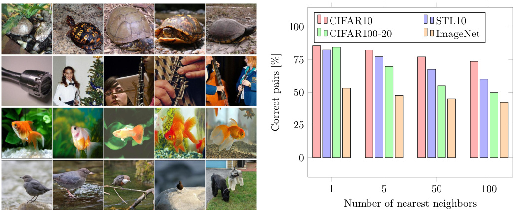
Fig. 1: Images (first column) and their Fig. 2: Neighboring samples tend to be nearest neighbors (other columns) [51]. instances of the same semantic class.
图 1: 图像(第一列)及其最近邻样本(其他列) [51]。
图 2: 相邻样本往往属于同一语义类别。
In representation learning, a pretext task $\tau$ learns in a self-supervised fashion an embedding function $\boldsymbol{\phi}_ {\theta}$ - parameterized by a neural network with weights $\theta$ - that maps images into feature representations. The literature offers several pretext tasks which can be used to learn such an embedding function $\boldsymbol{\phi}_ {\theta}$ (e.g. rotation prediction [16], affine or perspective transformation prediction [57], color iz ation [29], in-painting [39], instance discrimination [51,18,7,32], etc.). In practice, however, certain pretext tasks are based on specific image transformations, causing the learned feature representations to be covariant to the employed transformation. For example, when $\boldsymbol{\phi}_ {\theta}$ predicts the transformation parameters of an affine transformation, different affine transformations of the same image will result in distinct output predictions for $\boldsymbol{\phi}_ {\theta}$ . This renders the learned feature representations less appropriate for semantic clustering, where feature representations ought to be invariant to image transformations. To overcome this issue, we impose the pretext task $\tau$ to also minimize the distance between images $X_{i}$ and their augmentations $T[X_{i}]$ , which can be expressed as:
在表示学习中,前置任务 $\tau$ 以自监督方式学习一个嵌入函数 $\boldsymbol{\phi}_ {\theta}$ ——由权重为 $\theta$ 的神经网络参数化——将图像映射为特征表示。现有研究提出了多种可用于学习此类嵌入函数 $\boldsymbol{\phi}_ {\theta}$ 的前置任务(例如旋转预测 [16]、仿射或透视变换预测 [57]、着色 [29]、修复 [39]、实例判别 [51,18,7,32] 等)。然而实践中,某些前置任务基于特定图像变换,导致学到的特征表示会随所采用变换发生协变。例如当 $\boldsymbol{\phi}_ {\theta}$ 预测仿射变换参数时,同一图像的不同仿射变换会使 $\boldsymbol{\phi}_ {\theta}$ 产生不同的输出预测。这使得学到的特征表示不太适用于需要保持图像变换不变性的语义聚类任务。为解决该问题,我们要求前置任务 $\tau$ 同时最小化图像 $X_{i}$ 与其增强版本 $T[X_{i}]$ 之间的距离,可表示为:
$$
\operatorname*{min}_ {\theta}d(\varPhi_{\theta}(X_{i}),\varPhi_{\theta}(T[X_{i}])).
$$
$$
\operatorname*{min}_ {\theta}d(\varPhi_{\theta}(X_{i}),\varPhi_{\theta}(T[X_{i}])).
$$
Any pretext task [51,18,7,32] that satisfies Equation 1 can consequently be used. For example, Figure 1 shows the results when retrieving the nearest neighbors under an instance discrimination task [51] which satisfies Equation 1. We observe that similar features are assigned to semantically similar images. An experimental evaluation using different pretext tasks can be found in Section 3.2.
任何满足公式1的预训练任务[51,18,7,32]都可以使用。例如,图1展示了在满足公式1的实例判别任务[51]下检索最近邻的结果。我们观察到语义相似的图像被分配了相似的特征。使用不同预训练任务的实验评估见第3.2节。
To understand why images with similar high-level features are mapped closer together by $\boldsymbol{\phi}_ {\theta}$ , we make the following observations. First, the pretext task output is conditioned on the image, forcing $\boldsymbol{\phi}_ {\theta}$ to extract specific information from its input. Second, because $\phi_{\theta}$ has a limited capacity, it has to discard information from its input that is not predictive of the high-level pretext task. For example, it is unlikely that $\boldsymbol{\phi}_ {\theta}$ can solve an instance discrimination task by only encoding color or a single pixel from the input image. As a result, images with similar high-level characteristics will lie closer together in the embedding space of $\phi_{\theta}$ .
为了理解为何具有相似高级特征的图像会被 $\boldsymbol{\phi}_ {\theta}$ 映射到更接近的位置,我们进行了以下观察。首先,前置任务(pretext task)的输出以图像为条件,迫使 $\boldsymbol{\phi}_ {\theta}$ 从其输入中提取特定信息。其次,由于 $\phi_{\theta}$ 的容量有限,它必须舍弃输入中与高级前置任务预测无关的信息。例如,$\boldsymbol{\phi}_ {\theta}$ 不太可能仅通过编码输入图像的颜色或单个像素来解决实例判别任务。因此,具有相似高级特征的图像在 $\phi_{\theta}$ 的嵌入空间中会彼此更接近。
We conclude that pretext tasks from representation learning can be used to obtain semantically meaningful features. Following this observation, we will leverage the pretext features as a prior for clustering the images.
我们得出结论,表示学习(representation learning)中的前置任务可用于获取具有语义意义的特征。基于这一观察,我们将利用这些前置特征作为图像聚类的先验信息。
2.2 A semantic clustering loss
2.2 语义聚类损失
Mining nearest neighbors. In Section 2.1, we motivated that a pretext task from representation learning can be used to obtain semantically meaningful features. However, naively applying K-means on the obtained features can lead to cluster degeneracy [4]. A disc rim i native model can assign all its probability mass to the same cluster when learning the decision boundary. This leads to one cluster dominating the others. Instead, we opt for a better strategy.
挖掘最近邻。在2.1节中,我们提出表征学习中的前置任务可用于获取语义特征。但直接在所得特征上应用K-means可能导致聚类退化[4]。判别模型在学习决策边界时,可能将所有概率质量分配给同一聚类,导致单个聚类主导其他聚类。为此,我们选择了更优策略。
Let us first consider the following experiment. Through representation learning, we train a model $\boldsymbol{\phi}_ {\theta}$ on the unlabeled dataset $\mathcal{D}$ to solve a pretext task $\tau$ , i.e. instance discrimination [7,18]. Then, for every sample $X_{i}\in{\mathcal{D}}$ , we mine its $K$ nearest neighbors in the embedding space $\boldsymbol{\phi}_ {\theta}$ . We define the set $\mathcal{N}_ {X_{i}}$ as the neighboring samples of $X_{i}$ in the dataset $\mathcal{D}$ . Figure 2 quantifies the degree to which the mined nearest neighbors are instances of the same semantic cluster. We observe that this is largely the case across four datasets1 (CIFAR10 [27], CIFAR100-20 [27], STL10 [9] and ImageNet [11]) for different values of $K$ . Motivated by this observation, we propose to adopt the nearest neighbors obtained through the pretext task $\tau$ as our prior for semantic clustering.
首先考虑以下实验。通过表征学习,我们在未标注数据集 $\mathcal{D}$ 上训练模型 $\boldsymbol{\phi}_ {\theta}$ 来解决前置任务 $\tau$ (即实例判别 [7,18])。然后,对于每个样本 $X_{i}\in{\mathcal{D}}$,我们在嵌入空间 $\boldsymbol{\phi}_ {\theta}$ 中挖掘其 $K$ 个最近邻。将集合 $\mathcal{N}_ {X_{i}}$ 定义为数据集中 $X_{i}$ 的邻近样本。图 2 量化了所挖掘最近邻属于同一语义聚类实例的程度。我们观察到,在四个数据集 (CIFAR10 [27]、CIFAR100-20 [27]、STL10 [9] 和 ImageNet [11]) 中,对于不同的 $K$ 值,这一现象普遍存在。基于此观察,我们建议采用通过前置任务 $\tau$ 获得的最近邻作为语义聚类的先验。
Loss function. We aim to learn a clustering function $\phi_{\eta}$ - parameterized by a neural network with weights $\eta$ - that classifies a sample $X_{i}$ and its mined neighbors $\mathcal{N}_ {X_{i}}$ together. The function $\phi_{\eta}$ terminates in a softmax function to perform a soft assignment over the clusters $\mathcal{C}={1,\ldots,C}$ , with $\varPhi_{\eta}\left(X_{i}\right)\in$ $[0,1]^{C}$ . The probability of sample $X_{i}$ being assigned to cluster $c$ is denoted as $\varPhi_{\eta}^{c}(X_{i})$ . We learn the weights of $\phi_{\eta}$ by minimizing the following objective:
损失函数。我们的目标是学习一个聚类函数 $\phi_{\eta}$ ——由权重为 $\eta$ 的神经网络参数化——将样本 $X_{i}$ 及其挖掘的邻居 $\mathcal{N}_ {X_{i}}$ 一起分类。该函数 $\phi_{\eta}$ 以 softmax 函数结束,对聚类 $\mathcal{C}={1,\ldots,C}$ 进行软分配,其中 $\varPhi_{\eta}\left(X_{i}\right)\in$ $[0,1]^{C}$。样本 $X_{i}$ 被分配到聚类 $c$ 的概率表示为 $\varPhi_{\eta}^{c}(X_{i})$。我们通过最小化以下目标来学习 $\phi_{\eta}$ 的权重:
$$
\begin{array}{c}{{\displaystyle{\cal A}=-\frac{1}{|\mathcal{D}|}\sum_{X\in\mathcal{D}}\sum_{k\in\mathcal{N}_ {X}}\log\langle\varPhi_{\eta}(X),\varPhi_{\eta}(k)\rangle+\lambda\sum_{c\in\mathcal{C}}\varPhi_{\eta}^{\prime c}\log\varPhi_{\eta}^{\prime c},}}\ {{\mathrm{with~}\varPhi_{\eta}^{\prime c}=\displaystyle{\frac{1}{|\mathcal{D}|}\sum_{X\in\mathcal{D}}\varPhi_{\eta}^{c}(X)}.}}\end{array}
$$
$$
\begin{array}{c}{{\displaystyle{\cal A}=-\frac{1}{|\mathcal{D}|}\sum_{X\in\mathcal{D}}\sum_{k\in\mathcal{N}_ {X}}\log\langle\varPhi_{\eta}(X),\varPhi_{\eta}(k)\rangle+\lambda\sum_{c\in\mathcal{C}}\varPhi_{\eta}^{\prime c}\log\varPhi_{\eta}^{\prime c},}}\ {{\mathrm{with~}\varPhi_{\eta}^{\prime c}=\displaystyle{\frac{1}{|\mathcal{D}|}\sum_{X\in\mathcal{D}}\varPhi_{\eta}^{c}(X)}.}}\end{array}
$$
Here, $\langle\cdot\rangle$ denotes the dot product operator. The first term in Equation 2 imposes $\phi_{\eta}$ to make consistent predictions for a sample $X_{i}$ and its neighboring samples $\mathcal{N}_ {X_{i}}$ . Note that, the dot product will be maximal when the predictions are one-hot (confident) and assigned to the same cluster (consistent). To avoid $\phi_{\eta}$ from assigning all samples to a single cluster, we include an entropy term (the second term in Equation 2), which spreads the predictions uniformly across the clusters $\mathit{c}$ . If the probability distribution over the clusters $\mathcal{C}$ is known in advance, which is not the case here, this term can be replaced by KL-divergence.
这里,$\langle\cdot\rangle$表示点积运算符。公式2中的第一项要求$\phi_{\eta}$对样本$X_{i}$及其邻近样本$\mathcal{N}_ {X_{i}}$做出一致的预测。需要注意的是,当预测结果为独热编码(置信度高)且分配到同一聚类(一致)时,点积将达到最大值。为了防止$\phi_{\eta}$将所有样本分配到单一聚类,我们引入了一个熵项(公式2中的第二项),该熵项将预测均匀分布在聚类$\mathit{c}$上。如果事先已知聚类$\mathcal{C}$上的概率分布(此处并非如此),则可以用KL散度替代这一项。
Remember that, the exact number of clusters in $\mathcal{C}$ is generally unknown. However, similar to prior work [52,6,24], we choose $C$ equal to the number of ground-truth clusters for the purpose of evaluation. In practice, it should be possible to obtain a rough estimate of the amount of clusters2. Based on this estimate, we can over cluster to a larger amount of clusters, and enforce the class distribution to be uniform. We refer to Section 3.4 for a concrete experiment.
需要注意的是,集合 $\mathcal{C}$ 中的确切聚类数量通常是未知的。不过,与先前研究 [52,6,24] 类似,出于评估目的,我们选择将 $C$ 设定为真实聚类数量。实际应用中,应能对聚类数量进行粗略估计2。基于该估计值,我们可以过度聚类至更大数量的簇,并强制类别分布保持均匀。具体实验可参考第3.4节。
Implementation details. For the practical implementation of our loss function, we approximate the dataset statistics by sampling batches of sufficiently large size. During training we randomly augment the samples $X_{i}$ and their neighbors $\mathcal{N}_ {X_{i}}$ . For the corner case $K=0$ , only consistency between samples and their augmentations is imposed. We set $K\geq1$ to capture more of the cluster’s variance, at the cost of introducing noise, i.e. not all samples and their neighbors belong to the same cluster. Section 3.2 experimentally shows that choosing $K\geq1$ significantly improves the results compared to only enforcing consistency between samples and their augmentations, as in [24,21].
实现细节。在实际实现我们的损失函数时,我们通过采样足够大的批次来近似数据集统计量。训练过程中,我们随机对样本$X_{i}$及其邻域$\mathcal{N}_ {X_{i}}$进行数据增强。对于极端情况$K=0$,仅强制样本与其增强版本之间的一致性。我们设置$K\geq1$以捕获更多聚类方差,代价是引入噪声(即并非所有样本及其邻域都属于同一聚类)。第3.2节实验表明,与[24,21]中仅强制样本与其增强版本一致性的方法相比,选择$K\geq1$能显著提升结果。
Discussion. Unlike [40,25,49,2,34,59,52] we do not include a reconstruction criterion into the loss, since this is not explicitly required by our target task. After all, we are only interested in a few bits of information encoded from the input signal, rather than the majority of information that a reconstruction criterion typically requires. It is worth noting that the consistency in our case is enforced at the level of individual samples through the dot product term in the loss, rather than on an approximation of the joint distribution over the classes [24,21]. We argue that this choice allows to express the consistency in a more direct way.
讨论。与[40,25,49,2,34,59,52]不同,我们没有在损失函数中加入重建准则,因为我们的目标任务并不明确需要这一点。毕竟,我们只对从输入信号中编码的少量信息感兴趣,而不是重建准则通常需要的大部分信息。值得注意的是,在我们的方法中,一致性是通过损失函数中的点积项在单个样本级别上强制实现的,而不是通过对类别联合分布的近似[24,21]。我们认为这种选择能以更直接的方式表达一致性。
2.3 Fine-tuning through self-labeling
2.3 通过自标注进行微调
The semantic clustering loss in Section 2.2 imposed consistency between a sample and its neighbors. More specifically, each sample was combined with $K\geq1$ neighbors, some of which inevitably do not belong to the same semantic cluster. These false positive examples lead to predictions for which the network is less certain. At the same time, we experimentally observed that samples with highly confident predictions ( $p_{m a x}\approx1$ ) tend to be classified to the proper cluster. In fact, the highly confident predictions that the network forms during clustering can be regarded as ”prototypes” for each class (see Section 3.5). Unlike prior work [6,4,52], this allows us to select samples based on the confidence of the predictions in a more reliable manner. Hence, we propose a self-labeling approach [43,31,46] to exploit the already well-classified examples, and correct for mistakes due to noisy nearest neighbors.
第2.2节中的语义聚类损失强制样本与其邻居之间保持一致性。具体而言,每个样本会与$K\geq1$个邻居结合,其中部分邻居不可避免地不属于同一语义簇。这些假阳性样本会导致网络预测的不确定性增加。同时,我们通过实验观察到,预测置信度较高的样本( $p_{m a x}\approx1$ )往往能被正确归类到所属簇。实际上,网络在聚类过程中形成的高置信度预测可被视为每个类别的"原型"(参见第3.5节)。与先前工作[6,4,52]不同,这使我们能够以更可靠的方式基于预测置信度筛选样本。因此,我们提出一种自标注方法[43,31,46],利用已分类良好的样本来修正由噪声近邻导致的错误。
In particular, during training confident samples are selected by threshold ing the probability at the output, i.e. $p_{m a x}>$ threshold. For every confident sample, a pseudo label is obtained by assigning the sample to its predicted cluster. A cross-entropy loss is used to update the weights for the obtained pseudo labels. To avoid over fitting, we calculate the cross-entropy loss on strongly augmented versions of the confident samples. The self-labeling step allows the network to correct itself, as it gradually becomes more certain, adding more samples to the mix. We refer to Section 3.2 for a concrete experiment.
具体而言,在训练过程中,通过设定输出概率阈值筛选高置信度样本,即 $p_{max}>$ 阈值。每个高置信度样本会被分配至其预测簇以获得伪标签,随后使用交叉熵损失函数更新这些伪标签对应的权重。为防止过拟合,我们在强数据增强版本的高置信度样本上计算交叉熵损失。这种自标记机制使网络能够逐步自我修正——随着模型置信度提升,更多样本会被纳入训练流程。具体实验设置详见第3.2节。
Algorithm 1 summarizes all the steps of the proposed method. We further refer to it as SCAN, i.e. Semantic Clustering by Adopting Nearest neighbors.
算法1总结了所提出方法的所有步骤。我们进一步将其称为SCAN (Semantic Clustering by Adopting Nearest neighbors) 。
3 Experiments
3 实验
3.1 Experimental setup
3.1 实验设置
Datasets. The experimental evaluation is performed on CIFAR10 [27], CIFAR100- 20 [27], STL10 [9] and ImageNet [11]. We focus on the smaller datasets first. The results on ImageNet are discussed separately in Section 3.5. Some prior works [24,6,52,54] trained and evaluated on the complete datasets. Differently, we train and evaluate using the train and val split respectively. Doing so, allows to study the generalization properties of the method for novel unseen examples. Note that this does not result in any unfair advantages compared to prior work. The results are reported as the mean and standard deviation from 10 different runs. Finally, all experiments are performed using the same backbone, augmentations, pretext task and hyper parameters.
数据集。实验评估在 CIFAR10 [27]、CIFAR100-20 [27]、STL10 [9] 和 ImageNet [11] 上进行。我们首先关注较小的数据集,ImageNet 的结果将在 3.5 节单独讨论。先前部分研究 [24,6,52,54] 使用完整数据集进行训练和评估,而我们分别采用训练集和验证集进行训练与评估。这种方式能更好地研究该方法对未见样本的泛化特性,且不会造成与先前工作对比的不公平优势。所有结果均报告 10 次独立运行的平均值及标准差。实验均采用相同骨干网络、数据增强、前置任务和超参数完成。
Training setup. We use a standard ResNet-18 backbone. For every sample, the 20 nearest neighbors are determined through an instance discrimination task based on noise contrastive estimation (NCE) [51]. We adopt the SimCLR [7] imple ment ation for the instance discrimination task on the smaller datasets, and the implementation from MoCo [8] on ImageNet. The selected pretext task satisfies the feature invariance constraint from Equation 1 w.r.t. the transformations applied to augment the input images. In particular, every image is disentangled as a unique instance independent of the applied transformation. To speed up training, we transfer the weights, obtained from the pretext task to initiate the clustering step (Section 2.2). We perform the clustering step for 100 epochs using batches of size 128. The weight on the entropy term is set to $\lambda=5$ . A higher weight avoids the premature grouping of samples early on during training. The results seem to be insensitive to small changes of $\lambda$ . After the clustering step, we train for another 200 epochs using the self-labeling procedure with threshold 0.99 (Section 2.3). A weighted cross-entropy loss compensates for the imbalance between confident samples across clusters. The class weights are inversely proportional to the number of occurrences in the batch after threshold ing. The network weights are updated through Adam [25] with learning rate $10^{-4}$ and weight decay $10^{-4}$ . The images are strongly augmented by composing four randomly selected transformations from Rand Augment [10] during both the clustering and selflabeling steps. The transformation parameters are uniformly sampled between fixed intervals. For more details visit the supplementary materials.
训练设置。我们使用标准ResNet-18主干网络。对于每个样本,通过基于噪声对比估计(NCE) [51]的实例判别任务确定其20个最近邻。在较小数据集上采用SimCLR [7]实现的实例判别任务,在ImageNet上采用MoCo [8]的实现方案。所选前置任务满足公式1关于输入图像增强变换的特征不变性约束,其中每张图像被解耦为独立于所应用变换的独特实例。
为加速训练,我们将从前置任务获得的权重迁移至聚类步骤初始化(第2.2节)。聚类阶段使用128的批量大小进行100轮训练,熵项权重设置为$\lambda=5$。较高权重可避免训练早期样本过早分组,结果显示对$\lambda$微小变化不敏感。
完成聚类后,我们采用阈值为0.99的自标记程序(第2.3节)继续训练200轮。加权交叉熵损失用于补偿跨聚类置信样本的不平衡性,类别权重与阈值处理后批次中出现次数成反比。网络权重通过Adam [25]优化器更新,学习率$10^{-4}$,权重衰减$10^{-4}$。
在聚类和自标记阶段,图像均通过Rand Augment [10]中随机选取的四种变换进行强增强,变换参数在固定区间内均匀采样。更多细节详见补充材料。
Validation criterion During the clustering step, we select the best model based on the lowest loss. During the self-labeling step, we save the weights of the model when the amount of confident samples plateaus. We follow these practices as we do not have access to a labeled validation set.
验证标准
在聚类步骤中,我们根据最低损失选择最佳模型。在自标注步骤中,当置信样本数量趋于稳定时保存模型权重。由于无法使用带标注的验证集,我们遵循上述实践方法。
3.2 Ablation studies
3.2 消融实验
Method. We quantify the performance gains w.r.t. the different parts of our method through an ablation study on CIFAR10 in Table 1. K-means clustering of the NCE pretext features results in the lowest accuracy (65.9%), and is characterized by a large variance (5.7%). This is to be expected since the cluster assignments can be imbalanced (Figure 3), and are not guaranteed to align with the ground-truth classes. Interestingly, applying K-means to the pretext features outperforms prior state-of-the-art methods for unsupervised classification based on end-to-end learning schemes (see Sec. 3.3). This observation supports our primary claim, i.e. it is beneficial to separate feature learning from clustering. Updating the network weights through the SCAN-loss - while augmenting the input images through SimCLR transformations - outperforms K-means (+15.9%). Note that the SCAN-loss is somewhat related to K-means, since both methods employ the pretext features as their prior to cluster the images. Differently, our loss avoids the cluster degeneracy issue. We also research the effect of using different augmentation strategies during training. Applying transformations from RandA gu ment (RA) to both the samples and their mined neighbors further improves the performance (78.7% vs. 81.8%). We hypothesize that strong augmentations help to reduce the solution space by imposing additional in variances.
方法。我们通过在CIFAR10上的消融实验(表1)量化了方法各部分的性能提升。对NCE前置任务特征进行K-means聚类时准确率最低(65.9%)且方差较大(5.7%)。这是由于聚类分配可能不平衡(图3),且无法保证与真实类别对齐。值得注意的是,对前置特征应用K-means的表现优于当前基于端到端学习的无监督分类方法(见3.3节)。这一发现支持了我们的核心观点:将特征学习与聚类分离是有益的。通过SCAN-loss更新网络权重(同时采用SimCLR变换增强输入图像)比K-means提升了15.9%。需注意SCAN-loss与K-means存在关联,二者都利用前置特征作为聚类先验。不同的是,我们的损失函数避免了聚类退化问题。我们还研究了训练时采用不同增强策略的影响。对样本及其挖掘的邻居同时应用RandAugment(RA)变换可进一步提升性能(78.7% vs. 81.8%)。我们推测强增强能通过施加额外不变性来缩减解空间。
Fine-tuning the network through self-labeling further enhances the quality of the cluster assignments (81.8% to $87.6%$ ). During self-labeling, the network corrects itself as it gradually becomes more confident (see Figure 4). Importantly, in order for self-labeling to be successfully applied, a shift in augmentations is required (see Table 1 or Figure 5). We hypothesize that this is required to prevent the network from over fitting on already well-classified examples. Finally, Figure 6 shows that self-labeling procedure is not sensitive to the threshold’s value.
通过自标注 (self-labeling) 对网络进行微调可进一步提升聚类分配质量 (81.8% 提升至 $87.6%$)。在自标注过程中,随着网络置信度逐步提升,其会进行自我修正 (见图 4)。值得注意的是,成功应用自标注需要调整数据增强策略 (见表 1 或图 5)。我们推测这一调整能防止网络对已分类良好的样本产生过拟合。最后,图 6 表明自标注过程对阈值选择不敏感。
Table 1: Ablation Method CIFAR10
| Setup | ACC (Avg± Std) |
| Pretext+K-means | 65.9±5.7 |
| SCAN-Loss (SimCLR) | 78.7 ± 1.7 |
| Self-Labeling (SimCLR) | 10.0 ± 0 |
| (2) Self-Labeling (RA) | 87.4 ± 1.6 |
| SCAN-LoSS (RA) | 81.8 ± 1.7 |
| (1) Self-Labeling g(RA) | 87.6 ± 0.4 |
表 1: 消融方法 CIFAR10
| Setup | ACC (Avg± Std) |
|---|---|
| Pretext+K-means | 65.9±5.7 |
| SCAN-Loss (SimCLR) | 78.7 ± 1.7 |
| Self-Labeling (SimCLR) | 10.0 ± 0 |
| (2) Self-Labeling (RA) | 87.4 ± 1.6 |
| SCAN-LoSS (RA) | 81.8 ± 1.7 |
| (1) Self-Labeling g(RA) | 87.6 ± 0.4 |
Table 2: Ablation Pretext CIFAR10
| PretextTask | Clustering | ACC (Avg±Std) |
| RotNet [16] | K-means | 27.1±2.1 |
| Inst. discr. [51] | SCAN K-means | 74.3±3.9 52.0 ±4.6 |
| SCAN | 83.5 ± 4.1 | |
| K-means | 65.9±5.7 | |
| Inst. discr. [7] | SCAN | 87.6 ± 0.4 |
表 2: 消融实验预训练任务 CIFAR10
| PretextTask | Clustering | ACC (Avg±Std) |
|---|---|---|
| RotNet [16] | K-means | 27.1±2.1 |
| Inst. discr. [51] | SCAN K-means | 74.3±3.9 52.0 ±4.6 |
| SCAN | 83.5 ± 4.1 | |
| K-means | 65.9±5.7 | |
| Inst. discr. [7] | SCAN | 87.6 ± 0.4 |
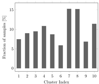
Fig. 3: K-means cluster assignments are imbalanced.
图 3: K-means聚类分配不均衡。
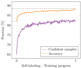
Fig. 4: Acc. and the number of confident samples during self-labeling.
图 4: 自标注过程中的准确率与高置信度样本数量。
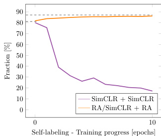
Fig. 5: Self-labeling with SimCLR or RandAugment augmentations.
图 5: 使用 SimCLR 或 RandAugment 增强的自标注方法。
Pretext task. We study the effect of using different pretext tasks to mine the nearest neighbors. In particular we consider two different implementations of the instance discrimination task from before [51,7], and RotNet [16]. The latter trains the network to predict image rotations. As a consequence, the distance between an image $X_{i}$ and its augmentations $T[X_{i}]$ is not minimized in the embedding space of a model pretrained through RotNet (see Equation 1). Differently, the instance disc ri mint ation task satisfies the invariance criterion w.r.t. the used augmentations. Table 2 shows the results on CIFAR10.
前置任务。我们研究了使用不同前置任务挖掘最近邻的效果。具体而言,我们考虑了此前[51,7]提出的实例判别(instance discrimination)任务的两种实现方式,以及RotNet[16]。后者通过训练网络预测图像旋转角度来实现特征学习。因此,在通过RotNet预训练的模型嵌入空间中,图像$X_{i}$与其增强版本$T[X_{i}]$之间的距离不会被最小化(参见公式1)。与之不同,实例判别任务能够满足数据增强的不变性准则。表2展示了在CIFAR10数据集上的实验结果。
First, we observe that the proposed method is not tied to a specific pretext task. All cases report high accuracy $\mathrm{\check{\Sigma}}>70%$ ). Second, pretext tasks that satisfy the invariance criterion are better suited to mine the nearest neighbors, i.e. $83.5%$ and 87.6% for inst. discr. versus $74.3%$ for RotNet. This confirms our hypothesis from Section 2.1, i.e. it is beneficial to choose a pretext task which imposes invariance between an image and its augmentations.
首先,我们观察到所提出的方法并不依赖于特定的前置任务。所有案例均报告了较高的准确率($\mathrm{\check{\Sigma}}>70%$)。其次,满足不变性准则的前置任务更适合挖掘最近邻,例如实例判别(inst. discr.)达到83.5%和87.6%,而RotNet为74.3%。这验证了我们在第2.1节的假设,即选择能对图像及其增强版本施加不变性的前置任务是有益的。
Number of neighbors. Figure 7 shows the influence of using a different number of nearest neighbors $K$ during the clustering step. The results are not very sensitive to the value of $K$ , and even remain stable when increasing $K$ to 50. This is beneficial, since we do not have to fine-tune the value of $K$ on very new dataset. In fact, both robustness and accuracy improve when increasing the value of $K$ upto a certain value. We also consider the corner case $K=0$ , when only enforcing consistent predictions for images and their augmentations. the performance decreases on all three datasets compared to $K=5$ , $56.3%$ vs $79.3%$ on CIFAR10, $24.6%$ vs $41.1%$ on CIFAR100-20 and $47.70%$ vs $69.8%$ on STL10. This confirms that better representations can be learned by also enforcing coherent predictions between a sample and its nearest neighbors.
邻居数量。图 7 展示了在聚类步骤中使用不同最近邻数量 $K$ 的影响。结果对 $K$ 值不太敏感,即使将 $K$ 增加到 50 仍能保持稳定。这非常有益,因为我们无需在新数据集上微调 $K$ 值。实际上,当 $K$ 值增加到一定程度时,鲁棒性和准确性都会提升。我们还考虑了极端情况 $K=0$(仅对图像及其增强版本强制一致预测),其性能在三个数据集上均低于 $K=5$ 的情况:CIFAR10 上 $56.3%$ 对比 $79.3%$,CIFAR100-20 上 $24.6%$ 对比 $41.1%$,STL10 上 $47.70%$ 对比 $69.8%$。这证实了通过强制样本与其最近邻之间的一致性预测,可以学习到更好的表征。
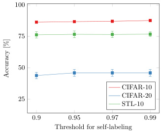
Fig. 6: Ablation thresh- old during self-labeling step.
图 6: 自标注步骤中的消融阈值。
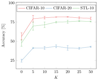
Fig. 7: Influence of the used number of neighbors $K$ .
图 7: 使用的邻居数量 $K$ 的影响
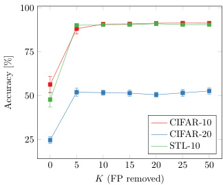
Fig. 8: Results without false positives in the nearest neighbors.
图 8: 最近邻中无假阳性的结果
Convergence. Figure 8 shows the results when removing the false positives from the nearest neighbors, i.e. sample-pairs which belong to a different class. The results can be considered as an upper-bound for the proposed method in terms of classification accuracy. A desirable characteristic is that the clusters quickly align with the ground truth, obtaining near fully-supervised performance on CIFAR10 and STL10 with a relatively small increase in the number of used neighbors $K$ . The lower performance improvement on CIFAR100-20 can be explained by the ambiguity of the super classes used to measure the accuracy. For example, there is not exactly one way to group categories like omnivores or carnivores together.
收敛性。图 8 展示了从最近邻中剔除假阳性(即属于不同类别的样本对)后的结果。该结果可视为所提方法在分类准确率方面的理论上限。一个理想特性是聚类结果能快速与真实类别对齐,在CIFAR10和STL10数据集上仅需少量增加近邻数量$K$即可接近全监督性能。CIFAR100-20数据集上性能提升较低,可归因于用于测量准确率的超类存在模糊性(例如将杂食动物或肉食动物等类别分组时并不存在唯一标准)。
3.3 Comparison with the state-of-the-art
3.3 与现有最优方法的对比
Comparison. Table 3 compares our method to the state-of-the-art on three different benchmarks. We evaluate the results based on clustering accuracy (ACC), normalized mutual information (NMI) and adjusted rand index (ARI). The proposed method consistently outperforms prior work by large margins on all three metrics, e.g. $+26.6%$ on CIFAR10, $+25.0%$ on CIFAR100-20 and $+21.3%$ on STL10 in terms of accuracy. We also compare with the state-of-the-art in representation learning [7] (Pretext $^+$ K-means). As shown in Section 3.2, our method outperforms the application of K-means on the pretext features. Finally, we also include results when tackling the problem in a fully-supervised manner. Our model obtains close to supervised performance on CIFAR-10 and STL-10. The performance gap is larger on CIFAR100-20, due to the use of super classes.
对比。表3将我们的方法与三种不同基准上的最先进技术进行了比较。我们基于聚类准确率(ACC)、归一化互信息(NMI)和调整兰德指数(ARI)评估结果。所提出的方法在所有三个指标上都大幅领先于先前工作,例如在CIFAR10上准确率提升$+26.6%$,在CIFAR100-20上提升$+25.0%$,在STL10上提升$+21.3%$。我们还与表征学习领域的最新技术[7] (Pretext$^+$K-means)进行了比较。如第3.2节所示,我们的方法优于在pretext特征上应用K-means的结果。最后,我们还包含了以全监督方式处理该问题的结果。我们的模型在CIFAR-10和STL-10上获得了接近监督学习的性能。由于使用了超类,在CIFAR100-20上的性能差距较大。
Table 3: State-of-the-art comparison: We report the averaged results for 10 different runs after the clustering ( $^*$ ) and self-labeling steps (†), and the best model. Opposed to prior work, we train and evaluate using the train and val split respectively, instead of using the full dataset for both training and testing.
| Dataset Metric | CIFAR10 | CIFAR100-20 | STL10 | ||||||
| ACC | NMI | ARI | ACC | NMI | ARI | ACC | NMI | ARI | |
| K-means [50] | 22.9 | 8.7 | 4.9 | 13.0 | 8.4 | 2.8 | 19.2 | 12.5 | 6.1 |
| SC [55] | 24.7 | 10.3 | 8.5 | 13.6 | 9.0 | 2.2 | 15.9 | 9.8 | 4.8 |
| Triplets [42] | 20.5 | 一 | 9.94 | 一 | 一 | 24.4 | 一 | ||
| JULE [54] | 27.2 | 19.2 | 13.8 | 13.7 | 10.3 | 3.3 | 27.7 | 18.2 | 16.4 |
| AEVB [26] | 29.1 | 24.5 | 16.8 | 15.2 | 10.8 | 4.0 | 28.2 | 20.0 | 14.6 |
| SAE [34] | 29.7 | 24.7 | 15.6 | 15.7 | 10.9 | 4.4 | 32.0 | 25.2 | 16.1 |
| DAE [49] | 29.7 | 25.1 | 16.3 | 15.1 | 11.1 | 4.6 | 30.2 | 22.4 | 15.2 |
| SWWAE [59] | 28.4 | 23.3 | 16.4 | 14.7 | 10.3 | 3.9 | 27.0 | 19.6 | 13.6 |
| AE [2] | 31.4 | 23.4 | 16.9 | 16.5 | 10.0 | 4.7 | 30.3 | 25.0 | 16.1 |
| GAN [40] | 31.5 | 26.5 | 17.6 | 15.1 | 12.0 | 4.5 | 29.8 | 21.0 | 13.9 |
| DEC [52] | 30.1 | 25.7 | 16.1 | 18.5 | 13.6 | 5.0 | 35.9 | 27.6 | 18.6 |
| ADC [17] | 32.5 | 16.0 | 一 | 一 | 53.0 | 一 | |||
| DeepCluster [4] | 37.4 | 18.9 | 一 | 一 | 33.4 | 一 | |||
| DAC [6] | 52.2 | 40.0 | 30.1 | 23.8 | 18.5 | 8.8 | 47.0 | 36.6 | 25.6 |
| IIC [24] | 61.7 | 51.1 | 41.1 | 25.7 | 22.5 | 11.7 | 59.6 | 49.6 | 39.7 |
| Supervised | 93.8 | 86.2 | 87.0 | 80.0 | 68.0 | 63.2 | 80.6 | 65.9 | 63.1 |
| Pretext [7]+ K-means | 65.9 ± 5.7 | 59.8 ± 2.0 | 50.9 ± 3.7 | 39.5 ± 1.9 | 40.2 ± 1.1 | 23.9 ± 1.1 | 65.8 ± 5.1 | 60.4 ± 2.5 | 50.6 ± 4.1 |
| SCAN*(Avg ± Std) | 81.8 ± 0.3 | 71.2 ± 0.4 | 66.5 ± 0.4 | 42.2 ± 3.0 | 44.1 ± 1.0 | 26.7 ± 1.3 | 75.5 ± 2.0 | 65.4 ± 1.2 | 59.0 ± 1.6 |
| SCANt (Avg ± Std) | 87.6 ± 0.4 | 78.7 ± 0.5 | 75.8 ± 0.7 | 45.9 ± 2.7 | 46.8 ± 1.3 | 30.1 ± 2.1 | 76.7 ± 1.9 | 68.0 ± 1.2 | 61.6 ± 1.8 |
| SCAN (Best) | 88.3 | 79.7 | 77.2 | 50.7 | 48.6 | 33.3 | 80.9 | 69.8 | 64.6 |
| SCANt(Overcluster) | 86.2 ± 0.8 77.1 ± 0.1 | 73.8 ± 1.4 | 55.1 ± 1.6 | 50.0 ± 1.1 | 35.7 ±1.7 | 76.8 ± 1.1 | 65.6 ± 0.8 | 58.6 ± 1.6 | |
表 3: 先进方法对比:我们报告了聚类 ( $^*$ ) 和自标注步骤 (†) 后 10 次不同运行的平均结果,以及最佳模型。与先前工作不同,我们分别使用训练集和验证集进行训练和评估,而非使用完整数据集同时进行训练和测试。
| 数据集指标 | CIFAR10 | CIFAR100-20 | STL10 | ||||||
|---|---|---|---|---|---|---|---|---|---|
| ACC | NMI | ARI | ACC | NMI | ARI | ACC | NMI | ARI | |
| K-means [50] | 22.9 | 8.7 | 4.9 | 13.0 | 8.4 | 2.8 | 19.2 | 12.5 | 6.1 |
| SC [55] | 24.7 | 10.3 | 8.5 | 13.6 | 9.0 | 2.2 | 15.9 | 9.8 | 4.8 |
| Triplets [42] | 20.5 | - | - | 9.94 | - | - | 24.4 | - | - |
| JULE [54] | 27.2 | 19.2 | 13.8 | 13.7 | 10.3 | 3.3 | 27.7 | 18.2 | 16.4 |
| AEVB [26] | 29.1 | 24.5 | 16.8 | 15.2 | 10.8 | 4.0 | 28.2 | 20.0 | 14.6 |
| SAE [34] | 29.7 | 24.7 | 15.6 | 15.7 | 10.9 | 4.4 | 32.0 | 25.2 | 16.1 |
| DAE [49] | 29.7 | 25.1 | 16.3 | 15.1 | 11.1 | 4.6 | 30.2 | 22.4 | 15.2 |
| SWWAE [59] | 28.4 | 23.3 | 16.4 | 14.7 | 10.3 | 3.9 | 27.0 | 19.6 | 13.6 |
| AE [2] | 31.4 | 23.4 | 16.9 | 16.5 | 10.0 | 4.7 | 30.3 | 25.0 | 16.1 |
| GAN [40] | 31.5 | 26.5 | 17.6 | 15.1 | 12.0 | 4.5 | 29.8 | 21.0 | 13.9 |
| DEC [52] | 30.1 | 25.7 | 16.1 | 18.5 | 13.6 | 5.0 | 35.9 | 27.6 | 18.6 |
| ADC [17] | 32.5 | - | - | 16.0 | - | - | 53.0 | - | - |
| DeepCluster [4] | 37.4 | - | - | 18.9 | - | - | 33.4 | - | - |
| DAC [6] | 52.2 | 40.0 | 30.1 | 23.8 | 18.5 | 8.8 | 47.0 | 36.6 | 25.6 |
| IIC [24] | 61.7 | 51.1 | 41.1 | 25.7 | 22.5 | 11.7 | 59.6 | 49.6 | 39.7 |
| Supervised | 93.8 | 86.2 | 87.0 | 80.0 | 68.0 | 63.2 | 80.6 | 65.9 | 63.1 |
| Pretext [7]+ K-means | 65.9 ± 5.7 | 59.8 ± 2.0 | 50.9 ± 3.7 | 39.5 ± 1.9 | 40.2 ± 1.1 | 23.9 ± 1.1 | 65.8 ± 5.1 | 60.4 ± 2.5 | 50.6 ± 4.1 |
| SCAN*(Avg ± Std) | 81.8 ± 0.3 | 71.2 ± 0.4 | 66.5 ± 0.4 | 42.2 ± 3.0 | 44.1 ± 1.0 | 26.7 ± 1.3 | 75.5 ± 2.0 | 65.4 ± 1.2 | 59.0 ± 1.6 |
| SCAN† (Avg ± Std) | 87.6 ± 0.4 | 78.7 ± 0.5 | 75.8 ± 0.7 | 45.9 ± 2.7 | 46.8 ± 1.3 | 30.1 ± 2.1 | 76.7 ± 1.9 | 68.0 ± 1.2 | 61.6 ± 1.8 |
| SCAN (Best) | 88.3 | 79.7 | 77.2 | 50.7 | 48.6 | 33.3 | 80.9 | 69.8 | 64.6 |
| SCAN†(过聚类) | - | 86.2 ± 0.8 | 77.1 ± 0.1 | 73.8 ± 1.4 | 55.1 ± 1.6 | 50.0 ± 1.1 | 35.7 ±1.7 | 76.8 ± 1.1 | 65.6 ± 0.8 |
Other advantages. In contrast to prior work [6,24,21], we did not have to perform any dataset specific fine-tuning. Furthermore, the results on CIFAR10 can be obtained within 6 hours on a single GPU. As a comparison, training the model from [24] requires at least a day of training time.
其他优势。与先前工作[6,24,21]不同,我们无需执行任何数据集特定微调。此外,CIFAR10上的结果可在单块GPU上6小时内获得。作为对比,训练文献[24]中的模型至少需要一整天时间。
3.4 Over clustering
3.4 过聚类
So far we assumed to have knowledge about the number of ground-truth classes. The method predictions were evaluated using a hungarian matching algorithm. However, what happens if the number of clusters does not match the number of ground-truth classes anymore. Table 3 reports the results when we overestimate the number of ground-truth classes by a factor of 2, e.g. we cluster CIFAR10 into 20 rather than 10 classes. The classification accuracy remains stable for CIFAR10 ( $87.6%$ to $86.2%$ ) and STL10 (76.7% to $76.8%$ ), and improves for CIFAR100-20 $(45.9%$ to $55.1%$ )3. We conclude that the approach does not require knowledge of the exact number of clusters. We hypothesize that the increased performance on CIFAR100-20 is related to the higher intra-class variance. More specifically, CIFAR100-20 groups multiple object categories together in super classes. In this case, an over clustering is better suited to explain the intra-class variance.
目前我们假设已知真实类别数量,并通过匈牙利匹配算法评估方法预测效果。但当聚类数量与真实类别数量不匹配时会发生什么?表3展示了当我们将真实类别数量高估两倍时的结果(例如将CIFAR10聚为20类而非10类)。分类准确率在CIFAR10(87.6%→86.2%)和STL10(76.7%→76.8%)保持稳定,在CIFAR100-20(45.9%→55.1%)有所提升[3]。这表明该方法无需预先知道精确的聚类数量。我们推测CIFAR100-20性能提升与其更高的类内方差有关:该数据集将多个物体类别归入超类,此时过度聚类能更好地解释类内方差。
Table 4: Validation set results for 50, 100 and 200 randomly selected classes from ImageNet. The results with K-means were obtained using the pretext features from MoCo [8]. We provide the results obtained by our method after the clustering step (∗), and after the self-labeling step (†).
| ImageNet Metric | 50Classes | 100 Classes | 200 Classes | |||||||||
| Top-1 | Top-5 | NMI | ARI | Top-1 | Top-5 | NMI | ARI | Top-1 | Top-5 | NMI | ARI | |
| K-means | 65.9 | 77.5 | 57.9 | 59.7 | 76.1 | 50.8 | 52.5 | 75.5 | 43.2 | |||
| SCAN* | 75.1 | 91.9 | 80.5 | 63.5 | 66.2 | 88.1 | 78.7 | 54.4 | 56.3 | 80.3 | 75.7 | 44.1 |
| SCANt | 76.8 | 91.4 | 82.2 | 66.1 | 68.9 | 86.1 | 80.8 | 57.6 | 58.1 | 80.6 | 77.2 | 47.0 |
表 4: 在ImageNet中随机选择50、100和200个类别的验证集结果。使用K-means方法得到的结果基于MoCo [8]的预训练特征。我们提供了聚类步骤后(∗)和自标注步骤后(†)通过我们的方法获得的结果。
| ImageNet指标 | 50类别 | 100类别 | 200类别 | |||||||||
|---|---|---|---|---|---|---|---|---|---|---|---|---|
| Top-1 | Top-5 | NMI | ARI | Top-1 | Top-5 | NMI | ARI | Top-1 | Top-5 | NMI | ARI | |
| K-means | 65.9 | 77.5 | 57.9 | 59.7 | 76.1 | 50.8 | 52.5 | 75.5 | 43.2 | |||
| SCAN* | 75.1 | 91.9 | 80.5 | 63.5 | 66.2 | 88.1 | 78.7 | 54.4 | 56.3 | 80.3 | 75.7 | 44.1 |
| SCAN† | 76.8 | 91.4 | 82.2 | 66.1 | 68.9 | 86.1 | 80.8 | 57.6 | 58.1 | 80.6 | 77.2 | 47.0 |
3.5 ImageNet
3.5 ImageNet
Setup. We consider the problem of unsupervised image classification on the large-scale ImageNet dataset [11]. We first consider smaller subsets of 50, 100 and 200 randomly selected classes. The sets of 50 and 100 classes are subsets of the 100 and 200 classes respectively. Additional details of the training setup can be found in the supplementary materials.
设置。我们在大规模ImageNet数据集[11]上研究无监督图像分类问题。首先选取50、100和200个随机类别的子集进行实验,其中50类和100类子集分别隶属于100类和200类子集。训练配置的更多细节可参阅补充材料。
Quantitative evaluation. Table 4 compares our results against applying Kmeans on the pretext features from MoCo [8]. Surprisingly, the application of K-means already performs well on this challenging task. We conclude that the pretext features are well-suited for the down-stream task of semantic clustering. Training the model with the SCAN-loss again outperforms the application of K-means. Also, the results are further improved when fine-tuning the model through self-labeling. We do not include numbers for the prior state-ofthe-art [24], since we could not obtain convincing results on ImageNet when running the publicly available code. We refer the reader to the supplementary materials for additional qualitative results on ImageNet-50.
定量评估。表4将我们的结果与在MoCo [8]的预训练特征上应用K均值聚类进行了对比。令人惊讶的是,K均值聚类在这个具有挑战性的任务上已经表现良好。我们得出结论,预训练特征非常适合语义聚类这一下游任务。使用SCAN-loss训练模型再次优于直接应用K均值聚类。此外,通过自标注进行微调后,结果得到进一步提升。我们没有包含先前最先进方法[24]的数据,因为在运行公开代码时未能在ImageNet上获得令人信服的结果。关于ImageNet-50的更多定性结果,请读者参阅补充材料。
Prototypical behavior. We visualize the different clusters after training the model with the SCAN-loss. Specifically, we find the samples closest to the mean embedding of the top-10 most confident samples in every cluster. The results are shown together with the name of the matched ground-truth classes in Fig. 9. Importantly, we observe that the found samples align well with the classes of the dataset, except for ’oboe’ and ’guacamole’ (red). Furthermore, the disc rim i native features of each object class are clearly present in the images. Therefore, we regard the obtained samples as ”prototypes” of the various clusters. Notice that the performed experiment aligns well with prototypical networks [45].
原型行为。我们通过SCAN-loss训练模型后对不同聚类簇进行可视化分析,具体方法是找出每个簇中置信度最高的前10个样本的均值嵌入最接近的样本。如图9所示,这些样本与匹配的真实类别名称共同呈现。值得注意的是,除"双簧管(oboe)"和"鳄梨酱(guacamole)"(红色标注)外,发现的样本与数据集类别高度吻合。此外,每个物体类别的判别性特征在图像中都清晰可见,因此我们将这些样本视为各聚类簇的"原型"。需要指出的是,该实验与原型网络[45]的研究结论高度一致。
ImageNet - 1000 classes. Finally, the model is trained on the complete ImageNet dataset. Figure 11 shows images from the validation set which were assigned to the same cluster by our model. The obtained clusters are semantically meaningful, e.g. planes, cars and primates. Furthermore, the clusters capture a large variety of different backgrounds, viewpoints, etc. We conclude that (to a large extent) the model predictions are invariant to image features which do not alter the semantics. On the other hand, based on the ImageNet ground-truth annotations, not all sample pairs should have been assigned to the same cluster. For example, the ground-truth annotations discriminate between different primates, e.g. chimpanzee, baboon, langur, etc. We argue that there is not a single correct way of categorizing the images according to their semantics in case of ImageNet. Even for a human annotator, it is not straightforward to cluster each image according to the ImageNet classes without prior knowledge.
ImageNet - 1000类。最终,模型在完整的ImageNet数据集上进行训练。图11展示了验证集中被我们的模型分配到同一簇的图像。获得的簇在语义上具有意义,例如飞机、汽车和灵长类动物。此外,这些簇涵盖了各种不同的背景、视角等。我们得出结论:(在很大程度上)模型预测对于不改变语义的图像特征是不变的。另一方面,根据ImageNet的真实标注,并非所有样本对都应该被分配到同一簇。例如,真实标注区分了不同的灵长类动物,如黑猩猩、狒狒、叶猴等。我们认为,在ImageNet的情况下,没有单一正确的方法可以根据语义对图像进行分类。即使对于人类标注者来说,在没有先验知识的情况下,根据ImageNet类别对每张图像进行聚类也并不简单。

Fig. 9: Prototypes obtained by sampling the confident samples.
图 9: 通过采样高置信度样本获得的原型。

Fig. 10: Zoom on seven super classes in the confusion matrix on ImageNet.
图 10: ImageNet混淆矩阵中七个超类的局部放大图。

Fig. 11: Clusters extracted by our model on ImageNet (more in supplementary).
图 11: 我们的模型在ImageNet上提取的聚类簇(更多结果见补充材料)。
Based on the ImageNet hierarchy we select class instances of the following super classes: dogs, insects, primates, snake, clothing, buildings and birds. Figure 10 shows a confusion matrix of the selected classes. The confusion matrix has a block diagonal structure. The results show that the mis classified examples tend to be assigned to other clusters from within the same superclass, e.g. the model confuses two different dog breeds. We conclude that the model has learned to group images with similar semantics together, while its prediction errors can be attributed to the lack of annotations which could disentangle the fine-grained differences between some classes.
基于ImageNet层级结构,我们选取了以下超类别的类实例:犬类、昆虫、灵长类、蛇类、服装、建筑物和鸟类。图10展示了所选类别的混淆矩阵。该混淆矩阵呈现块对角结构。结果表明,误分类样本往往被归入同一超类别下的其他聚类,例如模型会混淆两种不同犬种。由此可得出结论:该模型已学会将语义相似的图像归为一组,其预测误差可归因于缺乏能够区分某些类别间细粒度差异的标注数据。
Finally, Table 5 compares our method against recent semi-supervised learning approaches when using $1%$ of the images as labelled data. We obtain the following quantitative results on ImageNet: Top-1: 39.9%, Top-5: $60.0%$ , NMI: $72.0%$ , ARI: $27.5%$ . Our method outperforms several semi-supervised learning approaches, without using labels. This further demonstrates the strength of our approach.
最后,表5比较了在使用1%图像作为标记数据时,我们的方法与近期半监督学习方法的性能。在ImageNet数据集上获得以下量化结果:Top-1准确率39.9%、Top-5准确率60.0%、归一化互信息(NMI)72.0%、调整兰德指数(ARI)27.5%。我们的方法在无需使用标签的情况下,超越了多种半监督学习方法,这进一步证明了本方法的优势。
Table 5: Comparison with supervised, and semi-supervised learning methods using $1%$ of the labelled data on ImageNet.
| Method | Backbone | Labels | Top-1 | Top-5 |
| SupervisedBaseline | ResNet-50 | 25.4 | 48.4 | |
| Pseudo-Label | ResNet-50 | √ | 51.6 | |
| VAT + Entropy Min.[56] | ResNet-50 | √ | 47.0 | |
| InstDisc [51] | ResNet-50 | √ | 39.2 | |
| BigBiGAN [15] | ResNet-50(4x) | √ | 55.2 | |
| PIRL [32] | ResNet-50 | √ | 一 | 57.2 |
| CPC v2 [20] | ResNet-161 | √ | 52.7 | 77.9 |
| SimCLR [7] | ResNet-50 | √ | 48.3 | 75.5 |
| SCAN (s.ino) | ResNet-50 | x | 39.9 | 60.0 |
表 5: 使用 ImageNet 上 1% 标注数据与监督学习及半监督学习方法的对比
| 方法 | 主干网络 | 标签 | Top-1 | Top-5 |
|---|---|---|---|---|
| SupervisedBaseline | ResNet-50 | 25.4 | 48.4 | |
| Pseudo-Label | ResNet-50 | √ | 51.6 | |
| VAT + Entropy Min. [56] | ResNet-50 | √ | 47.0 | |
| InstDisc [51] | ResNet-50 | √ | 39.2 | |
| BigBiGAN [15] | ResNet-50(4x) | √ | 55.2 | |
| PIRL [32] | ResNet-50 | √ | 一 | 57.2 |
| CPC v2 [20] | ResNet-161 | √ | 52.7 | 77.9 |
| SimCLR [7] | ResNet-50 | √ | 48.3 | 75.5 |
| SCAN (s.ino) | ResNet-50 | x | 39.9 | 60.0 |
4 Conclusion
4 结论
We presented a novel framework to unsupervised image classification. The proposed approach comes with several advantages relative to recent works which adopted an end-to-end strategy. Experimental evaluation shows that the proposed method outperforms prior work by large margins, for a variety of datasets. Furthermore, positive results on ImageNet demonstrate that semantic clustering can be applied to large-scale datasets. Encouraged by these findings, we believe that our approach admits several extensions to other domains, e.g. semantic segmentation, semi-supervised learning and few-shot learning.
我们提出了一种无监督图像分类的新框架。相较于近期采用端到端策略的研究工作,该方法具有多项优势。实验评估表明,该方法在多种数据集上均以显著优势超越先前工作。此外,在ImageNet上取得的积极成果证明,语义聚类可应用于大规模数据集。这些发现激励我们相信,该方法可扩展至其他领域,例如语义分割、半监督学习和少样本学习。
Acknowledgment. The authors thankfully acknowledge support by Toyota via the TRACE project and MACCHINA (KU Leuven, C14/18/065). Furthermore, we would like to thank Xu Ji for her valuable insights and comments. Finally, we thank Kevis-Kokitsi Maninis, Jonas Heylen and Mark De Wolf for their feedback.
致谢。作者衷心感谢丰田汽车公司通过TRACE项目和MACCHINA (KU Leuven, C14/18/065) 提供的支持。此外,我们要感谢Xu Ji提出的宝贵见解与建议。最后,我们感谢Kevis-Kokitsi Maninis、Jonas Heylen和Mark De Wolf的反馈意见。
References
参考文献
Supplementary Material
补充材料
A Smaller datasets
更小的数据集
We include additional qualitative results on the smaller datasets, i.e. CIFAR10 [27], CIFAR100-20 [27] and STL10 [9]. We used the models from the state-of-the-art comparison.
我们在较小数据集上提供了额外的定性结果,包括 CIFAR10 [27]、CIFAR100-20 [27] 和 STL10 [9]。这些模型来自最先进的对比研究。
A.1 Prototypical examples
A.1 典型示例
Figure S1 visualizes a prototype image for every cluster on CIFAR10, CIFAR100- 20 and STL-10. The object of interest is clearly recognizable in the images. It is worth noting that the prototypical examples on CIFAR10 and STL10 can be matched with the ground-truth classes of the dataset. This is not the case for CIFAR100-20, e.g. bus and bicycle belong to the vehicles 1 ground-truth class. This behavior can be easily understood since CIFAR-20 makes use of super classes. As a consequence, it is difficult to explain the intra-class variance from visual appearance alone. Interestingly, we can reduce this mismatch through over clustering (see Sec 3.4.).
图 S1: 展示了CIFAR10、CIFAR100-20和STL-10数据集中每个聚类的一个原型图像。图像中感兴趣的对象清晰可辨。值得注意的是,CIFAR10和STL10上的原型示例可以与数据集的真实类别相匹配。而CIFAR100-20则不然,例如公共汽车和自行车同属于交通工具1这一真实类别。这种行为很容易理解,因为CIFAR-20利用了超类。因此,仅从视觉外观上解释类内差异较为困难。有趣的是,我们可以通过过度聚类来减少这种不匹配(见第3.4节)。

Fig. S1: Prototype images on the smaller datasets.
图 S1: 小型数据集上的原型图像。
A.2 Low confidence examples
A.2 低置信度示例
Figure S2 shows examples for which the network produces low confidence predictions. In most cases, it is hard to determine the correct class label. The difficult
图 S2: 展示了网络产生低置信度预测的示例。在大多数情况下,很难确定正确的类别标签。

Fig. S2: Low confidence predictions.
图 S2: 低置信度预测。
examples include objects which are: only partially visible, occluded, under bad lighting conditions, etc.
示例包括以下对象:仅部分可见、被遮挡、处于不良光照条件等。
B ImageNet
B ImageNet
B.1 Training setup
B.1 训练设置
We summarize the training setup for ImageNet below.
我们在下文中总结了ImageNet的训练设置。
Pretext Task Similar to our setup on the smaller datasets, we select instance discrimination as our pretext task. In particular, we use the implementation from MoCo [8]. We use a ResNet-50 model as backbone.
前置任务
与我们在较小数据集上的设置类似,我们选择实例判别 (instance discrimination) 作为前置任务。具体而言,我们采用 MoCo [8] 的实现方案,并以 ResNet-50 模型作为主干网络。
Clustering Step We freeze the backbone weights during the clustering step, and only train the final linear layer using the SCAN-loss. More specifically, we train ten separate linear heads in parallel. When initiating the self-labeling step, we select the head with the lowest loss to continue training. Every image is augmented using augmentations from SimCLR [7]. We reuse the entropy weight from before (5.0), and train with batches of size 512, 1024 and 1024 on the subsets of 50, 100 and 200 classes respectively. We use an SGD optimizer with momentum 0.9 and initial learning rate 5.0. The model is trained for 100 epochs. On the full ImageNet dataset, we increase the batch size and learning rate to 4096 and 30.0 respectively, and decrease the number of neighbors to 20.
聚类步骤
在聚类步骤中,我们冻结主干网络的权重,仅使用SCAN损失训练最终的线性层。具体而言,我们并行训练十个独立的线性头。在启动自标注步骤时,选择损失最低的头部继续训练。每张图像均通过SimCLR [7] 的增强方法进行数据增强。我们沿用之前的熵权重(5.0),并分别在50、100和200类子集上使用512、1024和1024的批次大小进行训练。采用动量0.9、初始学习率5.0的SGD优化器,训练100个周期。在完整ImageNet数据集上,我们将批次大小和学习率分别提升至4096和30.0,并将近邻数减少至20。
Self-Labeling Step We use the strong augmentations from Rand Augment to finetune the weights through self-labeling. The model weights are updated for 25 epochs using SGD with momentum 0.9. The initial learning rate is set to 0.03 and kept constant. Batches of size 512 are used. Importantly, the model weights are updated through an exponential moving average with $\alpha=0.999$ . We did not find it necessary to apply class balancing in the cross-entropy loss.
自标注步骤
我们使用 Rand Augment 中的强增强方法通过自标注微调权重。模型权重使用带动量 0.9 的 SGD 进行 25 轮更新,初始学习率设为 0.03 并保持恒定,批次大小为 512。关键的是,模型权重通过指数移动平均 (exponential moving average) 更新,其中 $\alpha=0.999$。我们发现无需在交叉熵损失中应用类别平衡。
B.2 ImageNet - Subsets
B.2 ImageNet - 子集
Confusion matrix Figure S3 shows a confusion matrix on the ImageNet-50 dataset. Most of the mistakes can be found between classes that are hard to disentangle, e.g. ’Giant Schnauzer’ and ’Flat-coated Retriever’ are both black dog breeds, ’Guacamole’ and ’Mashed Potato’ are both food, etc.
混淆矩阵
图 S3 展示了 ImageNet-50 数据集上的混淆矩阵。大部分错误出现在难以区分的类别之间,例如 "巨型雪纳瑞 (Giant Schnauzer)" 和 "平毛寻回犬 (Flat-coated Retriever)" 都是黑色犬种,"鳄梨酱 (Guacamole)" 和 "土豆泥 (Mashed Potato)" 均属于食物类别等。
Prototype examples Figure S4 shows a prototype image for every cluster on the ImageNet-50 subset. This figure extends Figure 9 from the main paper. Remarkably, the vast majority of prototype images can be matched with one of the ground-truth classes.
原型示例
图 S4 展示了 ImageNet-50 子集上每个聚类的原型图像。该图是对主论文中图 9 的扩展。值得注意的是,绝大多数原型图像都能与真实类别之一匹配。
Low confidence examples Figure S5 shows examples for which the model produces low confidence predictions on the ImageNet-50 subset. In a number of cases, the low confidence output can be attributed to multiple objects being visible in the scene. Other cases can be explained by the partial visibility of the object, distracting elements in the scene, or ambiguity of the object of interest.
低置信度示例
图 S5: 展示了模型在ImageNet-50子集上产生低置信度预测的示例。部分案例中,低置信度输出可归因于场景中存在多个物体。其他情况则可能由物体部分可见、场景中存在干扰元素或目标物体本身存在歧义导致。
B.3 ImageNet - Full
B.3 ImageNet - 完整版
We include additional qualitative results on the full ImageNet dataset. In particular, Figures S6, S7 and S8 show images from the validation set that were assigned to the same cluster. These can be viewed together with Figure 11 in the main paper. Additionally, we show some mistakes in Figure S9. The failure cases occur when the model focuses too much on the background, or when the network cannot easily discriminate between pairs of similarly looking images. However, in most cases, we can still attach some semantic meaning to the clusters, e.g. animals in cages, white fences.
我们在完整ImageNet数据集上补充了定性分析结果。具体而言,图S6、图S7和图S8展示了验证集中被分配到同一聚类的图像,可与主论文中的图11对照查看。此外,图S9展示了一些错误案例,这些失败案例主要发生在模型过度关注背景时,或是网络难以区分外观相似的图像对时。不过大多数情况下,我们仍能为聚类结果赋予语义含义(例如笼中动物、白色栅栏等)。
C Experimental setup
C 实验设置
C.1 Datasets
C.1 数据集
Different from prior work [24,6,52,54], we do not train and evaluate on the full datasets. Differently, we use the standard train-val splits to study the generalization properties of our models. Additionally, we report the mean and standard deviation on the smaller datasets. We would like to encourage future works to adopt this procedure as well. Table S1 provides an overview of the number of classes, the number of images and the aspect ratio of the used datasets. The selected classes on ImageNet-50, ImageNet-100 and ImageNet-200 can be found in our git repository.
与之前的工作[24,6,52,54]不同,我们并未在完整数据集上进行训练和评估。相反,我们采用标准训练-验证分割来研究模型的泛化特性。此外,我们在较小数据集上报告了均值和标准差。我们希望鼓励后续研究也采用这一流程。表S1概述了所用数据集的类别数量、图像数量及长宽比信息。ImageNet-50、ImageNet-100和ImageNet-200的选定类别可在我们的git代码库中查阅。

Fig. S3: Confusion matrix on ImageNet-50
图 S3: ImageNet-50 上的混淆矩阵
Table S1: Datasets overview
| Dataset | Classes | Trainimages | Valimages | Aspectratio |
| CIFAR10 | 10 | 50,000 | 10,000 | 32x32 |
| CIFAR100-20 | 20 | 50,000 | 10,000 | 32x32 |
| STL10 | 10 | 5,000 | 8,000 | 96x96 |
| ImageNet-50 | 50 | 64,274 | 2,500 | 224x224 |
| ImageNet-100 | 100 | 128,545 | 5,000 | 224x224 |
| ImageNet-200 | 200 | 256,558 | 10,000 | 224x224 |
| ImageNet | 1000 | 1,281,167 | 50,000 | 224x224 |
表 S1: 数据集概览
| 数据集 | 类别数 | 训练图像数 | 验证图像数 | 宽高比 |
|---|---|---|---|---|
| CIFAR10 | 10 | 50,000 | 10,000 | 32x32 |
| CIFAR100-20 | 20 | 50,000 | 10,000 | 32x32 |
| STL10 | 10 | 5,000 | 8,000 | 96x96 |
| ImageNet-50 | 50 | 64,274 | 2,500 | 224x224 |
| ImageNet-100 | 100 | 128,545 | 5,000 | 224x224 |
| ImageNet-200 | 200 | 256,558 | 10,000 | 224x224 |
| ImageNet | 1000 | 1,281,167 | 50,000 | 224x224 |

Fig. S4: Prototype images on ImageNet-50.
图 S4: ImageNet-50 上的原型图像。

Fig. S5: Low confidence examples on ImageNet-50.
图 S5: ImageNet-50 上的低置信度示例。
C.2 Augmentations
C.2 增强
As shown in our experiments, it is beneficial to apply strong augmentations during training. The strong augmentations were composed of four randomly selected transformations from Rand Augment [10], followed by Cutout [12]. The transformation parameters were uniformly sampled between fixed intervals. Table S2 provides a detailed overview. We applied an identical augmentation strategy across all datasets.
如实验所示,在训练过程中应用强数据增强(strong augmentations)是有益的。强数据增强由从Rand Augment [10]中随机选择的四种变换组成,随后进行Cutout [12]。变换参数在固定区间内均匀采样。表S2提供了详细概述。我们在所有数据集上应用了相同的数据增强策略。

Fig. S6: Example clusters of ImageNet-1000 (1).
图 S6: ImageNet-1000 的示例聚类 (1)。

Fig. S7: Example clusters of ImageNet-1000 (2).
图 S7: ImageNet-1000的示例聚类 (2)。

Fig. S8: Example clusters of ImageNet-1000 (3).
图 S8: ImageNet-1000 的示例聚类 (3)。

Fig. S9: Incorrect clusters of ImageNet-1000 predicted by our model.
图 S9: 我们的模型预测错误的ImageNet-1000聚类结果。
Table S2: List of transformations. The strong transformations are composed by randomly selecting four transformations from the list, followed by Cutout.
| Transformation | Parameter | Interval |
| Identity | ||
| Autocontrast | ||
| Equalize | ||
| Rotate | θ | [-30,30] |
| Solarize | T | [0,256] |
| Color | C | 0.05,0.95] |
| Contrast | C | 0.05,0.95] |
| Brightness | B | [0.05,0.95] |
| Sharpness | S | [0.05,0.95] |
| Shear X | R | [0.1,0.1] |
| Translation X | 入 | 0.1,0.1] |
| TranslationY | 入 | [0.1,0.1] |
| Posterize | B | [4,8] |
| Shear Y | R | [-0.1,0.1] |
表 S2: 变换列表。强变换由从列表中随机选择四种变换后接Cutout组成。
| 变换 | 参数 | 区间 |
|---|---|---|
| Identity | ||
| Autocontrast | ||
| Equalize | ||
| Rotate | θ | [-30,30] |
| Solarize | T | [0,256] |
| Color | C | [0.05,0.95] |
| Contrast | C | [0.05,0.95] |
| Brightness | B | [0.05,0.95] |
| Sharpness | S | [0.05,0.95] |
| Shear X | R | [0.1,0.1] |
| Translation X | 入 | [0.1,0.1] |
| Translation Y | 入 | [0.1,0.1] |
| Posterize | B | [4,8] |
| Shear Y | R | [-0.1,0.1] |
D Change Log
D 变更日志
The following changes were made since version 1:
自版本1以来的变更如下: