Linformer: Self-Attention with Linear Complexity
Linformer: 线性复杂度的自注意力机制
Sinong Wang, Belinda Z. Li, Madian Khabsa, Han Fang, Hao Ma Facebook AI, Seattle, WA {sinongwang, belindali, hanfang, mkhabsa, haom}@fb.com
Sinong Wang, Belinda Z. Li, Madian Khabsa, Han Fang, Hao Ma Facebook AI, Seattle, WA {sinongwang, belindali, hanfang, mkhabsa, haom}@fb.com
Abstract
摘要
Large transformer models have shown extraordinary success in achieving state-ofthe-art results in many natural language processing applications. However, training and deploying these models can be prohibitively costly for long sequences, as the standard self-attention mechanism of the Transformer uses ${\bar{O}}(n^{2})$ time and space with respect to sequence length. In this paper, we demonstrate that the self-attention mechanism can be approximated by a low-rank matrix. We further exploit this finding to propose a new self-attention mechanism, which reduces the overall self-attention complexity from $O(n^{2})$ to $O(n)$ in both time and space. The resulting linear transformer, the Linformer, performs on par with standard Transformer models, while being much more memory- and time-efficient.
大型Transformer模型在诸多自然语言处理应用中展现出卓越性能,屡创最先进成果。然而,针对长序列场景,训练和部署这类模型可能成本过高,因为标准Transformer的自注意力机制相对于序列长度需要消耗${\bar{O}}(n^{2})$级别的时间和空间复杂度。本文证明自注意力机制可通过低秩矩阵近似实现,并基于此发现提出新型自注意力机制——将整体复杂度从$O(n^{2})$降至$O(n)$级别(时间与空间维度)。由此产生的线性Transformer(Linformer)在保持与标准Transformer相当性能的同时,显著提升了内存和计算效率。
1 Introduction
1 引言
Transformer models (Vaswani et al., 2017) have become ubiquitous for wide variety of problems in natural language processing (NLP), including translation (Ott et al., 2018), text classification, question answering, among others (Raffel et al., 2019; Mohamed et al., 2019). Over the last couple of years, the number of parameters in state-of-the-art NLP transformers has grown drastically, from the original 340 million introduced in BERT-Large to 175 billion in GPT-3 (Brown et al., 2020). Although these large-scale models yield impressive results on wide variety of tasks, training and deploying such model are slow in practice. For example, the original BERT-Large model (Devlin et al., 2019) takes four days to train on 16 Cloud TPUs, and the recent GPT-3 (Brown et al., 2020) consumed orders of magnitude more petaflops / day to train compared to its predecessor, GPT-2 (Radford et al., 2019). Beyond training, deploying Transformer models to real world applications is also expensive, usually requiring extensive distillation (Hinton et al., 2015) or compression.
Transformer模型 (Vaswani et al., 2017) 已成为自然语言处理 (NLP) 领域各类任务的通用解决方案,包括翻译 (Ott et al., 2018)、文本分类、问答等 (Raffel et al., 2019; Mohamed et al., 2019)。过去几年间,最先进NLP Transformer模型的参数量从BERT-Large最初的3.4亿激增至GPT-3的1750亿 (Brown et al., 2020)。虽然这些大规模模型在各类任务上表现惊艳,但其训练和部署过程实际耗时极长。例如原始BERT-Large模型 (Devlin et al., 2019) 需要16个云端TPU训练四天,而最新GPT-3 (Brown et al., 2020) 的每日训练算力消耗相比前代GPT-2 (Radford et al., 2019) 高出了数量级。除训练外,将Transformer模型部署到实际应用中也成本高昂,通常需要大量蒸馏 (Hinton et al., 2015) 或压缩操作。
The main efficiency bottleneck in Transformer models is its self-attention mechanism. Here, each token’s representation is updated by attending to all other tokens in the previous layer. This operation is key for retaining long-term information, giving Transformers the edge over recurrent models on long sequences. However, attending to all tokens at each layer incurs a complexity of $O(n^{2})$ with respect to sequence length. Thus, in this paper, we seek to answer the question: can Transformer models be optimized to avoid this quadratic operation, or is this operation required to maintain strong performance?
Transformer模型的主要效率瓶颈在于其自注意力(self-attention)机制。该机制通过让每个token关注前一层所有其他token来更新其表征。这一操作是保留长期信息的关键,使Transformer在长序列任务上优于循环模型。然而,每层对所有token的关注会导致复杂度随序列长度呈$O(n^{2})$增长。因此,本文旨在回答:能否通过优化Transformer模型来避免这种平方级运算,或者说这一运算是否是维持强劲性能的必要条件?
Prior work has proposed several techniques for improving the efficiency of self-attention. One popular technique is introducing sparsity into attention layers (Child et al., 2019; Qiu et al., 2019; Beltagy et al., 2020) by having each token attend to only a subset of tokens in the whole sequence. This reduces the overall complexity of the attention mechanism to $O(n{\sqrt{n}})$ (Child et al., 2019). However, as shown in Qiu et al. (2019), this approach suffers from a large performance drop with limited efficiency gains, i.e., a $2%$ drop with only $20%$ speed up. More recently, the Reformer (Kitaev et al., 2020) used locally-sensitive hashing (LSH) to reduce the self-attention complexity to $O(n\log(n))$ . However, in practice, the Reformer’s efficiency gains only appear on sequences with length $>2048$ (Figure 5 in Kitaev et al. (2020)). Furthermore, the Reformer’s multi-round hashing approach actually increases the number of sequential operations, which further undermines their final efficiency gains.
先前的研究提出了多种提升自注意力 (self-attention) 效率的技术。一种流行的方法是通过让每个 token 仅关注整个序列中的部分 token 来引入稀疏性 (Child et al., 2019; Qiu et al., 2019; Beltagy et al., 2020),这将注意力机制的整体复杂度降低至 $O(n{\sqrt{n}})$ (Child et al., 2019)。但如 Qiu et al. (2019) 所示,这种方法在效率提升有限的情况下会导致性能显著下降,例如速度仅提升 20% 时性能下降 2%。最近,Reformer (Kitaev et al., 2020) 使用局部敏感哈希 (LSH) 将自注意力复杂度降至 $O(n\log(n))$。然而实际应用中,Reformer 的效率优势仅在序列长度超过 2048 时显现 (Kitaev et al. (2020) 中的图 5)。此外,Reformer 的多轮哈希策略实际上增加了串行操作次数,进一步削弱了其最终效率收益。
In this work, we introduce a novel approach for tackling the self-attention bottleneck in Transformers. Our approach is inspired by the key observation that self-attention is low rank. More precisely, we show both theoretically and empirically that the stochastic matrix formed by self-attention can be approximated by a low-rank matrix. Empowered by this observation, we introduce a novel mechanism that reduces self-attention to an $O(n)$ operation in both space- and time-complexity: we decompose the original scaled dot-product attention into multiple smaller attentions through linear projections, such that the combination of these operations forms a low-rank factorization of the original attention. A summary of runtimes for various Transformer architectures, including ours, can be found in Table 1.
在本工作中,我们提出了一种解决Transformer中自注意力(self-attention)瓶颈的新方法。该方法源于一个关键发现:自注意力具有低秩特性。具体而言,我们通过理论和实验证明,自注意力形成的随机矩阵可以用低秩矩阵近似。基于这一发现,我们设计了一种新机制,将自注意力的空间和时间复杂度降至$O(n)$:通过线性投影将原始缩放点积注意力分解为多个较小注意力,这些操作的组合构成了原始注意力的低秩分解。表1展示了包括本方法在内的多种Transformer架构的运行时间对比。
One predominant application of Transformers, that has seen the most gains, is using them as pretrained language models, whereby models are first pretrained with a language modeling objective on a large corpus, then finetuned on target tasks using supervised data (Devlin et al., 2019; Liu et al., 2019; Lewis et al., 2019). Following Devlin et al. (2019), we pretrain our model on BookCorpus (Zhu et al., 2015) plus English Wikipedia using masked-language-modeling objective. We observe similar pre training performance to the standard Transformer model. We then finetune our pretrained models on three tasks from GLUE (Wang et al., 2018) and one sentiment analysis task, IMDB reviews (Maas et al., 2011). On these tasks, we find that our model performs comparably, or even slightly better, than the standard pretrained Transformer, while observing significant training and inference speedups.
Transformer最具成效的主流应用之一是将其作为预训练语言模型,即先在大规模语料库上以语言建模为目标进行预训练,再使用监督数据对目标任务进行微调 (Devlin et al., 2019; Liu et al., 2019; Lewis et al., 2019)。参照Devlin et al. (2019) 的方法,我们在BookCorpus (Zhu et al., 2015) 和英文维基百科上采用掩码语言建模目标进行预训练,观察到与标准Transformer模型相当的预训练性能。随后,我们在GLUE (Wang et al., 2018) 的三个任务和一个情感分析任务(IMDB影评数据集 (Maas et al., 2011))上对预训练模型进行微调。实验表明,在显著提升训练和推理速度的同时,我们的模型性能与标准预训练Transformer相当甚至略有优势。
| ModelArchitecture | Complexity per Layer | Sequential Operation |
| Recurrent | O(n) | O(n) |
| Transformer, (Vaswani et al.,2017) | O(n | 0(1) |
| Sparse Tansformer, (Child et al., 2019) | O(nv n | 0(1) |
| Reformer,(Kitaev et al.,2020) | O(nlog(n)) | O(log(n)) |
| Linformer | O(n) | 0(1) |
| 模型架构 (Model Architecture) | 单层复杂度 (Complexity per Layer) | 顺序操作 (Sequential Operation) |
|---|---|---|
| 循环网络 (Recurrent) | O(n) | O(n) |
| Transformer (Vaswani 等, 2017) | O(n | O(1) |
| 稀疏 Transformer (Child 等, 2019) | O(n√n | O(1) |
| Reformer (Kitaev 等, 2020) | O(nlog(n)) | O(log(n)) |
| Linformer | O(n) | O(1) |
Table 1: Per-layer time complexity and minimum number of sequential operations as a function of sequence length $(n)$ for various architectures.
表 1: 不同架构下各层时间复杂度与最小串行操作数随序列长度 $(n)$ 的变化关系。
2 Backgrounds and Related works
2 背景与相关工作
2.1 Transformer and Self-Attention
2.1 Transformer 与自注意力机制
The Transformer is built upon the idea of Multi-Head Self-Attention (MHA), which allows the model to jointly attend to information at different positions from different representation subspaces. MHA is defined as
Transformer 基于多头自注意力 (Multi-Head Self-Attention, MHA) 机制构建,该机制使模型能够同时关注来自不同表示子空间的多位置信息。MHA 定义为
$$
\mathrm{MultiHead}(Q,K,V)=\mathrm{Concat}(\mathrm{head}_ {1},\mathrm{head}_ {2},\dots,\mathrm{head}_{h})W^{O},
$$
$$
\mathrm{MultiHead}(Q,K,V)=\mathrm{Concat}(\mathrm{head}_ {1},\mathrm{head}_ {2},\dots,\mathrm{head}_{h})W^{O},
$$
where $Q,K,V\in\mathbb{R}^{n\times d_{m}}$ are input embedding matrices, $n$ is sequence length, $d_{m}$ is the embedding dimension, and $h$ is the number of heads. Each head is defined as:
其中 $Q,K,V\in\mathbb{R}^{n\times d_{m}}$ 是输入嵌入矩阵,$n$ 为序列长度,$d_{m}$ 为嵌入维度,$h$ 为注意力头数。每个注意力头的定义为:
$$
\mathrm{head}_ {i}=\mathrm{Attention}(Q W_{i}^{Q},K W_{i}^{K},V W_{i}^{V})=\underbrace{\mathrm{softmax}\left[\frac{Q W_{i}^{Q}(K W_{i}^{K})^{T}}{\sqrt{d_{k}}}\right]}_ {P}V W_{i}^{V},
$$
$$
\mathrm{head}_ {i}=\mathrm{Attention}(Q W_{i}^{Q},K W_{i}^{K},V W_{i}^{V})=\underbrace{\mathrm{softmax}\left[\frac{Q W_{i}^{Q}(K W_{i}^{K})^{T}}{\sqrt{d_{k}}}\right]}_ {P}V W_{i}^{V},
$$
where $\begin{array}{r}{W_{i}^{Q},W_{i}^{K}\in\mathbb{R}^{d_{m}\times d_{k}},W_{i}^{V}\in\mathbb{R}^{d_{m}\times d_{v}},W^{O}\in\mathbb{R}^{h d_{v}\times d_{m}}}\end{array}$ are learned matrices and $d_{k},d_{v}$ are the hidden dimensions of the projection subspaces. For the rest of this paper, we will not differentiate between $d_{k}$ and $d_{v}$ and just use $d$ .
其中 $\begin{array}{r}{W_{i}^{Q},W_{i}^{K}\in\mathbb{R}^{d_{m}\times d_{k}},W_{i}^{V}\in\mathbb{R}^{d_{m}\times d_{v}},W^{O}\in\mathbb{R}^{h d_{v}\times d_{m}}}\end{array}$ 是可学习矩阵,$d_{k},d_{v}$ 是投影子空间的隐藏维度。在本文后续部分,我们将不再区分 $d_{k}$ 和 $d_{v}$,统一使用 $d$。
The self-attention defined in (2) refers to a context mapping matrix $P\in\mathbb{R}^{n\times n}$ . The Transformer uses $P$ to capture the input context for a given token, based on a combination of all tokens in the sequence. However, computing $P$ is expensive. It requires multiplying two $n\times d$ matrices, which is $O(n^{2})$ in time and space complexity. This quadratic dependency on the sequence length has become a bottleneck for Transformers.
(2) 式中定义的自注意力 (self-attention) 涉及一个上下文映射矩阵 $P\in\mathbb{R}^{n\times n}$。Transformer 利用 $P$ 基于序列中所有 token 的组合来捕获给定 token 的输入上下文。然而,计算 $P$ 的成本很高:需要将两个 $n\times d$ 矩阵相乘,其时间和空间复杂度均为 $O(n^{2})$。这种对序列长度的二次依赖已成为 Transformer 的性能瓶颈。
2.2 Related works
2.2 相关工作
There has been much prior literature on improving the efficiency of Transformers, especially the self-attention bottleneck. The most common techniques for model efficiency that can be applied to Transformers (some specific to Transformers, others more general-purpose) include:
已有大量文献探讨如何提升Transformer的效率,尤其是解决自注意力机制的性能瓶颈。适用于Transformer的模型效率优化技术(部分专为Transformer设计,部分具有普适性)主要包括:
Mixed Precision (Mic ike vici us et al., 2017): Using half-precision or mixed-precision representations of floating points is popular in deep learning, and is also widely used in training Transformers (Ott et al., 2019). This technique can be further improved through Quantization Aware Training (Jacob et al., 2018; Fan et al., 2020), where the weights are quantized during training and the gradients are approximated with the Straight-Through Estimator. This line of work is orthogonal to our approach, and we use mixed-precision training by default.
混合精度 (Micikevicius et al., 2017): 在深度学习中,使用半精度或混合精度表示浮点数非常普遍,这种方法也广泛应用于训练Transformer (Ott et al., 2019)。该技术可通过量化感知训练 (Jacob et al., 2018; Fan et al., 2020) 进一步优化,即在训练过程中对权重进行量化,并通过直通估计器近似梯度。这类工作与我们的方法正交,默认情况下我们采用混合精度训练。
Knowledge Distillation (Hinton et al., 2015): Knowledge distillation aims to transfer the “knowledge" from a large teacher model to a lightweight student model. The student model is then used during inference. However this approach has drawbacks: It does not address speeding up the teacher model during training, and moreover, student models usually suffer performance degradation compared to the teacher model. For example, when distilling a 12-layer BERT to a 6-layer BERT, the student model experiences an average 2.5% performance drop on several benchmark tasks (Sanh et al., 2019).
知识蒸馏 (Hinton et al., 2015): 知识蒸馏旨在将大型教师模型中的"知识"迁移到轻量级学生模型中。推理阶段则使用学生模型。但该方法存在缺陷:它无法加速教师模型的训练过程,且学生模型性能通常低于教师模型。例如,将12层BERT蒸馏为6层BERT时,学生模型在多项基准任务上的平均性能下降达2.5% (Sanh et al., 2019)。
Sparse Attention (Child et al., 2019): This technique improves the efficiency of self-attention by adding sparsity in the context mapping matrix $P$ . For example, the Sparse Transformer (Child et al., 2019) only computes $P_{i j}$ around the diagonal of matrix $P$ (instead of the all $P_{i j}$ ). Meanwhile, blockwise self-attention (Qiu et al., 2019) divides $P$ into multiple blocks and only computes $P_{i j}$ within the selected blocks. However, these techniques also suffer a large performance degradation, while having only limited additional speed-up, i.e., 2% drop with 20% speed up.
稀疏注意力 (Child et al., 2019): 该技术通过在上下文映射矩阵 $P$ 中引入稀疏性来提升自注意力机制的效率。例如,稀疏Transformer (Child et al., 2019) 仅计算矩阵 $P$ 对角线附近的 $P_{i j}$ (而非全部 $P_{i j}$)。同时,分块自注意力 (Qiu et al., 2019) 将 $P$ 划分为多个块,仅计算选定块内的 $P_{i j}$。然而这些技术在仅获得有限加速 (如速度提升20%时性能下降2%) 的同时,也会导致显著的性能下降。
LSH Attention (Kitaev et al., 2020): Locally-sensitive hashing (LSH) attention utilizes a multi-round hashing scheme when computing dot-product attention, which in theory reduces the self-attention complexity to $O(n\log(n))$ . However, in practice, their complexity term has a large constant $128^{2}$ and it is only more efficient than the vanilla transformer when sequence length is extremely long.
LSH Attention (Kitaev et al., 2020): 局部敏感哈希 (Locally-sensitive Hashing, LSH) 注意力机制在计算点积注意力时采用多轮哈希方案,理论上可将自注意力复杂度降至 $O(n\log(n))$ 。但实际应用中,其复杂度项存在较大常数 $128^{2}$ ,仅当序列长度极长时才会比标准 Transformer 更高效。
Improving Optimizer Efficiency: Micro batching (Huang et al., 2019) splits a batch into small micro batches (which can be fit into memory), and then separately runs forward and backward passes on them with gradient accumulation. Gradient check pointing (Chen et al., 2016) saves memory by only caching activation s of a subset of layers. The uncached activation s are recomputed during back propagation from the latest checkpoint. Both techniques trade off time for memory, and do not speed up inference.
提升优化器效率:微批次处理 (Huang et al., 2019) 将批次拆分为小型微批次(可装入内存),并通过梯度累积分别执行前向和反向传播。梯度检查点 (Chen et al., 2016) 通过仅缓存部分层的激活值来节省内存,未缓存的激活值在反向传播时从最新检查点重新计算。这两种技术以时间换取内存,但不会加速推理。
As we’ve noted, most common techniques have limitations in reducing both the training and inference time/memory consumption, we investigate how to optimize the self-attention layers and introduce our approach next.
正如我们提到的,大多数常见技术在同时降低训练和推理时间/内存消耗方面存在局限,接下来我们将探讨如何优化自注意力(self-attention)层并介绍我们的方法。
3 Self-Attention is Low Rank
3 自注意力机制是低秩的
In this section, we demonstrate that the self-attention mechanism, i.e., the context mapping matrix $P$ , is low-rank.
在本节中,我们证明自注意力机制 (self-attention mechanism) ,即上下文映射矩阵 $P$ ,是低秩的。
We first provide a spectrum analysis of the context mapping matrix $P$ . We use two pretrained transformer models, RoBERTa-base (12-layer stacked transformer) and RoBERTa-large (24-layer stacked transformer) (Liu et al., 2019) on two tasks: masked-language-modeling task on Wiki103 (Merity et al., 2016) and classification task on IMDB (Maas et al., 2011). In Figure 1 (left), we apply singular value decomposition into $P$ across different layers and different heads of the model, and plot the normalized cumulative singular value averaged over 10k sentences. The results exhibit a clear long-tail spectrum distribution across each layer, head and task. This implies that most of the information of matrix $P$ can be recovered from the first few largest singular values. In Figure 1 (right), we plot a heatmap of the normalized cumulative singular value at the 128-th largest singular value (out of 512). We observe that the spectrum distribution in higher layers is more skewed than in lower layers, meaning that, in higher layers, more information is concentrated in the largest singular values and the rank of $P$ is lower.
我们首先对上下文映射矩阵 $P$ 进行谱分析。我们使用两个预训练的Transformer模型——RoBERTa-base(12层堆叠Transformer)和RoBERTa-large(24层堆叠Transformer)(Liu et al., 2019),在两个任务上进行实验:Wiki103 (Merity et al., 2016) 的掩码语言建模任务和IMDB (Maas et al., 2011) 的分类任务。在图1(左)中,我们对模型不同层和不同注意力头的 $P$ 进行奇异值分解,并绘制了10k个句子平均的归一化累积奇异值曲线。结果显示,每一层、每个注意力头和每个任务都呈现出明显的长尾谱分布。这表明矩阵 $P$ 的大部分信息可以通过前几个最大的奇异值恢复。在图1(右)中,我们绘制了第128大奇异值(共512个)处的归一化累积奇异值热力图。我们观察到,较高层的谱分布比较低层的更加偏斜,这意味着在较高层中,更多信息集中在最大的奇异值上,且 $P$ 的秩更低。
Below, we provide a theoretical analysis of the above spectrum results.
下面我们对上述频谱结果进行理论分析。
Theorem 1. (self-attention is low rank) For any $Q,K,V\in\mathbb{R}^{n\times d}$ and $W_{i}^{Q},W_{i}^{K},W_{i}^{V}\in\mathbb{R}^{d\times d}$ , for any column vector $w\in\mathbb{R}^{n}$ of matrix $V W_{i}^{V}$ , there exists a low-rank matrix $\tilde{P}\in\mathbb{R}^{n\times n}$ such that
定理1. (自注意力是低秩的) 对于任意 $Q,K,V\in\mathbb{R}^{n\times d}$ 和 $W_{i}^{Q},W_{i}^{K},W_{i}^{V}\in\mathbb{R}^{d\times d}$ ,对于矩阵 $V W_{i}^{V}$ 的任意列向量 $w\in\mathbb{R}^{n}$ ,存在一个低秩矩阵 $\tilde{P}\in\mathbb{R}^{n\times n}$ 使得
$\begin{array}{r}{\operatorname*{Pr}(|\tilde{P}w^{T}-P w^{T}|<\epsilon|P w^{T}|)>1-o(1)a n d~r a n k(\tilde{P})=\Theta(\log(n)),}\end{array}$ where the context mapping matrix $P$ is defined in (2).
$\begin{array}{r}{\operatorname*{Pr}(|\tilde{P}w^{T}-P w^{T}|<\epsilon|P w^{T}|)>1-o(1)a n d~r a n k(\tilde{P})=\Theta(\log(n)),}\end{array}$,其中上下文映射矩阵 $P$ 的定义见式 (2)。
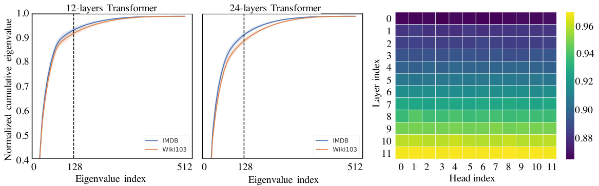
Figure 1: Left two figures are spectrum analysis of the self-attention matrix in pretrained transformer model (Liu et al., 2019) with $n=512$ . The Y-axis is the normalized cumulative singular value of context mapping matrix $P$ , and the X-axis the index of largest eigenvalue. The results are based on both RoBERTa-base and large model in two public datasets: Wiki103 and IMDB. The right figure plots the heatmap of normalized cumulative eigenvalue at the 128-th largest eigenvalue across different layers and heads in Wiki103 data.
图 1: 左侧两图展示了预训练Transformer模型 (Liu et al., 2019) 中自注意力矩阵的频谱分析 ($n=512$)。Y轴表示上下文映射矩阵 $P$ 的归一化累积奇异值,X轴为最大特征值索引。结果基于RoBERTa-base和large模型在Wiki103与IMDB两个公开数据集上的表现。右图呈现了Wiki103数据中不同层和注意力头在第128大特征值处的归一化累积特征值热力图。
Proof. Based on the definition of the context mapping matrix $P$ , we can write
证明。根据上下文映射矩阵 $P$ 的定义,我们可以写出
$$
P=\mathrm{softmax}\underbrace{\left[\frac{Q W_{i}^{Q}(K W_{i}^{K})^{T}}{\sqrt{d}}\right]}_ {A}=\exp{(A)}\cdot D_{A}^{-1},
$$
$$
P=\mathrm{softmax}\underbrace{\left[\frac{Q W_{i}^{Q}(K W_{i}^{K})^{T}}{\sqrt{d}}\right]}_ {A}=\exp{(A)}\cdot D_{A}^{-1},
$$
where $D_{A}$ is an $n\times n$ diagonal matrix. The main idea of this proof is based on the distribution al Johnson–Linden strauss lemma (Linden strauss, 1984) $\mathrm{JL}$ for short). We construct the approximate low rank matrix as $\tilde{P}=\exp\left(A\right)\cdot D_{A}^{-1}R^{T}R$ , where $R\in\mathbb{R}^{k\times n}$ with i.i.d. entries from $N(0,1/k)$ . We can then use the $\mathrm{JL}$ lemma to show that, for any column vector $w\in\mathbb{R}^{n}$ of matrix $V W_{i}^{V}$ , when $k=5\log(n)/(\epsilon^{2}-\epsilon^{3})$ , we have
其中 $D_{A}$ 是一个 $n\times n$ 的对角矩阵。该证明的主要思路基于分布式的 Johnson-Lindenstrauss 引理 (Lindenstrauss, 1984) (简称 $\mathrm{JL}$ )。我们构造近似低秩矩阵为 $\tilde{P}=\exp\left(A\right)\cdot D_{A}^{-1}R^{T}R$ ,其中 $R\in\mathbb{R}^{k\times n}$ 的条目独立同分布于 $N(0,1/k)$ 。随后可利用 $\mathrm{JL}$ 引理证明:对于矩阵 $V W_{i}^{V}$ 的任意列向量 $w\in\mathbb{R}^{n}$ ,当 $k=5\log(n)/(\epsilon^{2}-\epsilon^{3})$ 时,满足
$$
\operatorname*{Pr}\big(|P R^{T}R w^{T}-P w^{T}|\leq\epsilon|P w^{T}|\big)>1-o(1).
$$
$$
\operatorname*{Pr}\big(|P R^{T}R w^{T}-P w^{T}|\leq\epsilon|P w^{T}|\big)>1-o(1).
$$
For more details, refer to the supplementary materials.
更多详情请参阅补充材料。
Given the low-rank property of the context mapping matrix $P$ , one straightforward idea is to use singular value decomposition (SVD) to approximate $P$ with a low-rank matrix $P_{\mathrm{low}}$ , as follows
考虑到上下文映射矩阵 $P$ 的低秩特性,一个直观的想法是使用奇异值分解 (SVD) 来用低秩矩阵 $P_{\mathrm{low}}$ 近似 $P$,具体如下
$$
P\approx P_{\mathrm{low}}=\sum_{i=1}^{k}\sigma_{i}u_{i}v_{i}^{T}=\underbrace{\left[u_{1},\cdots,u_{k}\right]}_{k}\mathrm{diag}{\sigma_{1},\cdots,\sigma_{k}}\left[\begin{array}{c}{{v_{1}}}\ {{\vdots}}\ {{v_{k}}}\end{array}\right]\xi_{k}
$$
$$
P\approx P_{\mathrm{low}}=\sum_{i=1}^{k}\sigma_{i}u_{i}v_{i}^{T}=\underbrace{\left[u_{1},\cdots,u_{k}\right]}_{k}\mathrm{diag}{\sigma_{1},\cdots,\sigma_{k}}\left[\begin{array}{c}{{v_{1}}}\ {{\vdots}}\ {{v_{k}}}\end{array}\right]\xi_{k}
$$
where $\sigma_{i},u_{i}$ and $v_{i}$ are the $i$ largest singular values and their corresponding singular vectors. Based on the results in Theorem 1 and the Eckart–Young–Mirsky Theorem (Eckart & Young, 1936), one can use $P_{\mathrm{low}}$ to approximate self-attention (2) with $\epsilon$ error and $O(n k)$ time and space complexity. However, this approach requires performing an SVD decomposition in each self-attention matrix, which adds additional complexity. Therefore, we propose another approach for low-rank approximation that avoids this added complexity.
其中 $\sigma_{i},u_{i}$ 和 $v_{i}$ 分别是第 $i$ 大的奇异值及其对应的奇异向量。根据定理1的结果和Eckart-Young-Mirsky定理 (Eckart & Young, 1936),可以使用 $P_{\mathrm{low}}$ 以 $\epsilon$ 误差和 $O(n k)$ 的时间空间复杂度来近似自注意力机制 (2)。然而,这种方法需要对每个自注意力矩阵进行SVD分解,增加了额外的复杂度。因此,我们提出了另一种低秩近似方法以避免这种额外的复杂度。
4 Model
4 模型
In this section, we propose a new self-attention mechanism which allows us to compute the contextual mapping $P\cdot V W_{i}^{\hat{V}}$ in linear time and memory complexity with respect to sequence length.
在本节中,我们提出了一种新的自注意力机制 (self-attention mechanism) ,能够以序列长度的线性时间和内存复杂度计算上下文映射 $P\cdot V W_{i}^{\hat{V}}$ 。
The main idea of our proposed linear self-attention (Figure 2) is to add two linear projection matrices $E_{i},F_{i}\in\mathbb{R}^{n\times k}$ when computing key and value. We first project the original $(n\times d)$ -dimensional
我们提出的线性自注意力(图 2)的核心思想是在计算键和值时添加两个线性投影矩阵 $E_{i},F_{i}\in\mathbb{R}^{n\times k}$。我们首先对原始的 $(n\times d)$ 维
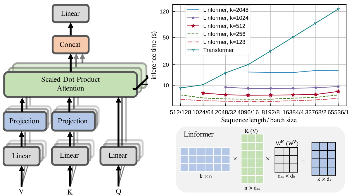
Figure 2: Left and bottom-right show architecture and example of our proposed multihead linear self-attention. Top right shows inference time vs. sequence length for various Linformer models.
图 2: 左侧和右下方展示了我们提出的多头线性自注意力 (multihead linear self-attention) 架构及示例。右上方展示了不同 Linformer 模型的推理时间与序列长度的关系。
key and value layers $K W_{i}^{K}$ and $V W_{i}^{V}$ into $(k\times d)$ -dimensional projected key and value layers. We then compute an $(n\times k)$ -dimensional context mapping matrix $\bar{P}$ using scaled dot-product attention.
键值层 $K W_{i}^{K}$ 和 $V W_{i}^{V}$ 投影为 $(k\times d)$ 维的键值层。随后通过缩放点积注意力计算 $(n\times k)$ 维的上下文映射矩阵 $\bar{P}$。
$$
\begin{array}{r l}&{\overline{{\mathrm{head}_ {i}}}=\mathrm{Attention}(Q W_{i}^{Q},E_{i}K W_{i}^{K},F_{i}V W_{i}^{V})}\ &{\qquad\quad=\underbrace{\mathrm{softmax}\left(\frac{Q W_{i}^{Q}(E_{i}K W_{i}^{K})^{T}}{\sqrt{d_{k}}}\right)}_ {\bar{P}:n\times k}\cdot\underbrace{F_{i}V W_{i}^{V}}_{k\times d},}\end{array}
$$
$$
\begin{array}{r l}&{\overline{{\mathrm{head}_ {i}}}=\mathrm{Attention}(Q W_{i}^{Q},E_{i}K W_{i}^{K},F_{i}V W_{i}^{V})}\ &{\qquad\quad=\underbrace{\mathrm{softmax}\left(\frac{Q W_{i}^{Q}(E_{i}K W_{i}^{K})^{T}}{\sqrt{d_{k}}}\right)}_ {\bar{P}:n\times k}\cdot\underbrace{F_{i}V W_{i}^{V}}_{k\times d},}\end{array}
$$
Finally, we compute context embeddings for each he $\operatorname{ad}_ {i}$ using $\bar{P}\cdot(F_{i}V W_{i}^{V})$ . Note the above operations only require $O(n k)$ time and space complexity. Thus, if we can choose a very small projected dimension $k$ , such that $k\ll n$ , then we can significantly reduce the memory and space consumption. The following theorem states that, when $\bar{k}={\cal O}(d/\epsilon^{2})$ (independent of $n$ ), one can approximate $P\cdot V W_{i}^{V}$ using linear self-attention (7) with $\epsilon$ error.
最后,我们使用 $\bar{P}\cdot(F_{i}V W_{i}^{V})$ 为每个 $\operatorname{ad}_ {i}$ 计算上下文嵌入。注意上述操作仅需 $O(n k)$ 的时间和空间复杂度。因此,若选择极小的投影维度 $k$ (满足 $k\ll n$),便能显著降低内存和空间消耗。以下定理表明:当 $\bar{k}={\cal O}(d/\epsilon^{2})$ (与 $n$ 无关)时,可通过线性自注意力(7)以 $\epsilon$ 误差逼近 $P\cdot V W_{i}^{V}$。
Theorem 2. (Linear self-attention) For any $Q_{i},K_{i},V_{i}\in\mathbb{R}^{n\times d}$ and $W_{i}^{Q},W_{i}^{K},W_{i}^{V}\in\mathbb{R}^{d\times d},$ , $i f$ $k=\operatorname*{min}{\Theta(9d\log(d)/\epsilon^{2}),5\Theta(\log(n)/\epsilon^{2})}$ , then there exists matrices $E_{i},F_{i}\in\mathbb{R}^{n\times k}$ such that, for any row vector $w$ of matrix $Q W_{i}^{Q}(K W_{i}^{K})^{T}/\sqrt{d},$ , we have
定理2. (线性自注意力) 对于任意 $Q_{i},K_{i},V_{i}\in\mathbb{R}^{n\times d}$ 和 $W_{i}^{Q},W_{i}^{K},W_{i}^{V}\in\mathbb{R}^{d\times d},$ 若 $k=\operatorname*{min}{\Theta(9d\log(d)/\epsilon^{2}),5\Theta(\log(n)/\epsilon^{2})}$ ,则存在矩阵 $E_{i},F_{i}\in\mathbb{R}^{n\times k}$ 使得对于矩阵 $Q W_{i}^{Q}(K W_{i}^{K})^{T}/\sqrt{d},$ 的任意行向量 $w$ ,满足
$$
\operatorname*{Pr}\left(\lVert\operatorname{softmax}(w E_{i}^{T})F_{i}V W_{i}^{V}-\operatorname{softmax}(w)V W_{i}^{V}\rVert\le\epsilon\lVert\operatorname{softmax}(w)\rVert\lVert V W_{i}^{V}\rVert\right)>1-o(1)
$$
$$
\operatorname*{Pr}\left(\lVert\operatorname{softmax}(w E_{i}^{T})F_{i}V W_{i}^{V}-\operatorname{softmax}(w)V W_{i}^{V}\rVert\le\epsilon\lVert\operatorname{softmax}(w)\rVert\lVert V W_{i}^{V}\rVert\right)>1-o(1)
$$
Proof. The main idea of proof is based on the distribution al Johnson–Linden strauss lemma (Lindenstrauss, 1984). We first prove that for any row vector $x\in\mathbb{R}^{n}$ of matrix $Q W_{i}^{Q}(K W_{i}^{K})^{T}/\sqrt{d_{k}}$ and column vector $y\in\mathbb{R}^{n}$ of matrix $V W_{i}^{V}$ ,
证明。该证明的主要思路基于分布型 Johnson-Lindenstrauss 引理 (Lindenstrauss, 1984)。我们首先证明对于矩阵 $Q W_{i}^{Q}(K W_{i}^{K})^{T}/\sqrt{d_{k}}$ 的任意行向量 $x\in\mathbb{R}^{n}$ 和矩阵 $V W_{i}^{V}$ 的列向量 $y\in\mathbb{R}^{n}$,
$$
\operatorname*{Pr}\left(|\exp(x E_{i}^{T})F_{i}y^{T}-\exp(x)y^{T}|\leq\epsilon|\exp(x)y^{T}|\right)>1-2e^{-(\epsilon^{2}-\epsilon^{3})k/4},
$$
$$
\operatorname*{Pr}\left(|\exp(x E_{i}^{T})F_{i}y^{T}-\exp(x)y^{T}|\leq\epsilon|\exp(x)y^{T}|\right)>1-2e^{-(\epsilon^{2}-\epsilon^{3})k/4},
$$
where $E_{i}=\delta R$ and $\begin{array}{r}{F_{i}=e^{-\delta}R}\end{array}$ , where $R\in\mathbb{R}^{k\times n}$ with i.i.d. entries from $N(0,1/k)$ and $\delta$ is a small constant. Applying the result in (9) to every row vector of matrix $A$ and every column vector of matrix $V$ , one can directly prove that, for any row vector $A_{i}$ of matrix $A$ ,
其中 $E_{i}=\delta R$ 且 $\begin{array}{r}{F_{i}=e^{-\delta}R}\end{array}$,其中 $R\in\mathbb{R}^{k\times n}$ 的条目独立同分布于 $N(0,1/k)$,$\delta$ 为小常数。将 (9) 式结果应用于矩阵 $A$ 的每个行向量和矩阵 $V$ 的每个列向量时,可直接证明:对于矩阵 $A$ 的任意行向量 $A_{i}$,
$$
\begin{array}{r}{\operatorname*{Pr}\left(|\exp(A_{i}E_{i}^{T})F_{i}V-\exp(A_{i})V|\leq\epsilon|\exp(A_{i})V|\right)>1-o(1),}\end{array}
$$
$$
\begin{array}{r}{\operatorname*{Pr}\left(|\exp(A_{i}E_{i}^{T})F_{i}V-\exp(A_{i})V|\leq\epsilon|\exp(A_{i})V|\right)>1-o(1),}\end{array}
$$
by setting $k=5\log(n d)/(\epsilon^{2}-\epsilon^{3})$ . This result does not utilize the low rank property of matrix $A$ $(\operatorname{rank}(A){=}d)$ and the resultant $k$ has a dependency on sequence length $n$ . We will further utlize the fact that rank $(A){=}d$ to prove the choice of $k$ can be constant and independent of sequence length $n$ . For more details, refer to the supplementary materials. 口
通过设定 $k=5\log(n d)/(\epsilon^{2}-\epsilon^{3})$ 。该结果未利用矩阵 $A$ 的低秩特性 $(\operatorname{rank}(A){=}d)$ ,且所得 $k$ 与序列长度 $n$ 存在依赖关系。我们将进一步利用矩阵秩 $(A){=}d$ 的特性,证明 $k$ 的取值可为常数且独立于序列长度 $n$ 。更多细节详见补充材料。口
In Figure 2 (top right), we plot the inference speed of Linformer and standard Transformer versus sequence length, while holding the total number of tokens fixed. We see that while standard Transformer becomes slower at longer sequence lengths, the Linformer speed remains relatively flat and is significantly faster at long sequences.
在图 2 (右上) 中,我们绘制了 Linformer 和标准 Transformer 在保持总 token 数不变时,推理速度随序列长度的变化曲线。可以看出,标准 Transformer 在较长序列时速度变慢,而 Linformer 的速度保持相对平稳,且在长序列时明显更快。
Additional Efficiency Techniques Several additional techniques can be introduced on top of Linformer to further optimize for both performance and efficiency:
附加效率优化技术
在Linformer基础上可引入多项技术进一步优化性能和效率:
Parameter sharing between projections: One can share parameters for the linear projection matrices $E_{i},F_{i}$ across layers and heads. In particular, we experimented with 3 levels of sharing:
投影间的参数共享:可以在不同层和头之间共享线性投影矩阵 $E_{i},F_{i}$ 的参数。具体而言,我们尝试了3种共享级别:
For example, in a 12-layer, 12-head stacked Transformer model, headwise sharing, key-value sharing and layerwise sharing will introduce 24, 12, and 1 distinct linear projection matrices, respectively.
例如,在一个12层、12头的堆叠式Transformer模型中,头间共享(headwise sharing)、键值共享(key-value sharing)和层间共享(layerwise sharing)将分别引入24、12和1个不同的线性投影矩阵。
Nonuniform projected dimension: One can choose a different projected dimension $k$ for different heads and layers. As shown in Figure 1 (right), the contextual mapping matrices in different heads and layers have distinct spectrum distributions, and heads in higher layer tend towards a more skewed distributed spectrum (lower rank). This implies one can choose a smaller projected dimension $k$ for higher layers.
非均匀投影维度:可以为不同注意力头和层选择不同的投影维度$k$。如图1 (右)所示,不同头和层中的上下文映射矩阵具有不同的频谱分布,更高层的头往往呈现更偏斜的频谱分布(更低秩)。这意味着可以为更高层选择更小的投影维度$k$。
General projections: One can also choose different kinds of low-dimensional projection methods instead of a simple linear projection. For example, one can choose mean/max pooling, or convolution where the kernel and stride is set to $n/k$ . The convolutional functions contain parameters that require training.
通用投影方法:除了简单的线性投影外,还可以选择不同类型的低维投影方法。例如,可选择均值/最大池化 (mean/max pooling) ,或卷积核与步长设置为 $n/k$ 的卷积操作。其中卷积函数包含需要训练的参数。
5 Experiments
5 实验
In this section, we present experimental results for the the techniques described above. We analyze the techniques one-by-one and explore how they impact performance.
在本节中,我们将展示上述技术的实验结果。我们将逐一分析这些技术,并探讨它们如何影响性能。
5.1 Pre training Perplexities
5.1 预训练困惑度
We first compare the pre training performance of our proposed architecture against RoBERTa (Liu et al., 2019), which is based on the Transformer. Following Devlin et al. (2019), we use BookCorpus (Zhu et al., 2015) plus English Wikipedia as our pre training set (3300M words). All models are pretrained with the masked-language-modeling (MLM) objective, and the training for all experiments are parallel i zed across 64 Tesla V100 GPUs with $250\mathrm{k}$ updates.
我们首先将提出的架构与基于Transformer的RoBERTa (Liu等人, 2019) 进行预训练性能对比。参照Devlin等人 (2019) 的方法,我们使用BookCorpus (Zhu等人, 2015) 加英文维基百科作为预训练集 (3300M词)。所有模型均采用掩码语言建模 (MLM) 目标进行预训练,所有实验均通过64块Tesla V100 GPU并行化训练,共进行$250\mathrm{k}$次参数更新。
Effect of projected dimension: We experiment with various values for the projected dimension $k$ . (We use the same $k$ across all layers and heads of Linformer.) In the Figure 3(a) and (b), we plot the validation perplexity curves for both the standard Transformer and the Linformer across different $k$ , for maximum sequence lengths $n=512$ and $n=1024$ . As expected, the Linformer performs better as projected dimension $k$ increases. However, even at $k=128$ for $n=512$ and $k=256$ for $n=1024$ , Linformer’s performance is already nearly on par with the original Transformer. Effect of sharing projections: In Figure 3(c), we plot the validation perplexity curves for the three parameter sharing strategies (headwise, key-value, and layerwise) with $n=512$ . Note that when we use just a single projection matrix (i.e. for layerwise sharing), the resulting Linformer model’s validation perplexity almost matches that of the the non-shared model. This suggests that we can decrease the number of additional parameters in our model, and consequently, it’s memory consumption, without much detriment to performance.
投影维度的影响:我们尝试了不同投影维度 $k$ 的取值(在Linformer的所有层和注意力头中保持相同的 $k$)。在图3(a)和(b)中,我们绘制了标准Transformer和Linformer在不同 $k$ 值下的验证困惑度曲线,最大序列长度分别为 $n=512$ 和 $n=1024$。正如预期,随着投影维度 $k$ 的增加,Linformer表现更好。然而,即使当 $n=512$ 时 $k=128$ 和 $n=1024$ 时 $k=256$,Linformer的性能已接近原始Transformer。
投影共享的影响:在图3(c)中,我们绘制了三种参数共享策略(头共享、键值共享和层共享)在 $n=512$ 时的验证困惑度曲线。值得注意的是,当仅使用单个投影矩阵(即层共享)时,Linformer模型的验证困惑度几乎与非共享模型相当。这表明我们可以减少模型中的额外参数数量,从而降低内存消耗,而不会显著影响性能。
Effect of longer sequences: We evaluate the effect of sequence length during Linformer pre training. In the Figure 3(d), we plot the validation perplexity for Linformer with $n\in{\bar{5}12,1024,2\bar{0}48,4096}$ holding projected dimension $k$ fixed at 256. Note that as sequence length increases, even though our projected dimension is fixed, the final perplexities after convergence remain about the same. This further empirically supports our assertion that the Linformer is linear-time.
更长序列的影响:我们评估了Linformer预训练中序列长度的影响。在图3(d)中,我们绘制了当投影维度$k$固定为256时,序列长度$n\in{\bar{5}12,1024,2\bar{0}48,4096}$下Linformer的验证困惑度。值得注意的是,随着序列长度的增加,尽管我们的投影维度保持不变,收敛后的最终困惑度基本相当。这进一步从实证角度支持了Linformer具有线性时间复杂度的论断。

Figure 3: Pre training validation perplexity versus number of updates.
图 3: 预训练验证困惑度与更新次数的关系。
| n | Model | SST-2 | IMDB | QNLI | QQP | Average |
| Liu et al.(2019),RoBERTa-base | 93.1 | 94.1 | 90.9 | 90.9 | 92.25 | |
| Linformer,128 | 92.4 | 94.0 | 90.4 | 90.2 | 91.75 | |
| Linformer, 128, shared kv | 93.4 | 93.4 | 90.3 | 90.3 | 91.85 | |
| Linformer,128,sharedkv,layer | 93.2 | 93.8 | 90.1 | 90.2 | 91.83 | |
| Linformer, 256 | 93.2 | 94.0 | 90.6 | 90.5 | 92.08 | |
| Linformer, 256, shared kv | 93.3 | 93.6 | 90.6 | 90.6 | 92.03 | |
| Linformer, 256, shared kv, layer | 93.1 | 94.1 | 91.2 | 90.8 | 92.30 | |
| 512 | Devlin et al.(2019),BERT-base | 92.7 | 93.5 | 91.8 | 89.6 | 91.90 |
| Sanh et al. (2019),Distilled BERT | 91.3 | 92.8 | 89.2 | 88.5 | 90.45 | |
| 1024 | Linformer, 256 | 93.0 | 93.8 | 90.4 | 90.4 | 91.90 |
| Linformer, 256, shared kv | 93.0 | 93.6 | 90.3 | 90.4 | 91.83 | |
| Linformer,256,sharedkv,layer | 93.2 | 94.2 | 90.8 | 90.5 | 92.18 |
| n | 模型 | SST-2 | IMDB | QNLI | QQP | 平均 |
|---|---|---|---|---|---|---|
| Liu et al. (2019), RoBERTa-base | 93.1 | 94.1 | 90.9 | 90.9 | 92.25 | |
| Linformer, 128 | 92.4 | 94.0 | 90.4 | 90.2 | 91.75 | |
| Linformer, 128, shared kv | 93.4 | 93.4 | 90.3 | 90.3 | 91.85 | |
| Linformer, 128, shared kv, layer | 93.2 | 93.8 | 90.1 | 90.2 | 91.83 | |
| Linformer, 256 | 93.2 | 94.0 | 90.6 | 90.5 | 92.08 | |
| Linformer, 256, shared kv | 93.3 | 93.6 | 90.6 | 90.6 | 92.03 | |
| Linformer, 256, shared kv, layer | 93.1 | 94.1 | 91.2 | 90.8 | 92.30 | |
| 512 | Devlin et al. (2019), BERT-base | 92.7 | 93.5 | 91.8 | 89.6 | 91.90 |
| 512 | Sanh et al. (2019), Distilled BERT | 91.3 | 92.8 | 89.2 | 88.5 | 90.45 |
| 1024 | Linformer, 256 | 93.0 | 93.8 | 90.4 | 90.4 | 91.90 |
| 1024 | Linformer, 256, shared kv | 93.0 | 93.6 | 90.3 | 90.4 | 91.83 |
| 1024 | Linformer, 256, shared kv, layer | 93.2 | 94.2 | 90.8 | 90.5 | 92.18 |
Table 2: Dev set results on benchmark natural language understanding tasks. The RoBERTa-base model here is pretrained with same corpus as BERT.
表 2: 基准自然语言理解任务开发集结果。此处的 RoBERTa-base 模型采用与 BERT 相同的语料库进行预训练。
5.2 Downstream Results
5.2 下游任务结果
Thus far, we have only examined the pre training perplexities of our model. However, we wish to show that our conclusions hold after finetuning on downstream tasks. We finetune our Linformer on IMDB (Maas et al., 2011) and SST-2 (Socher et al., 2013) (sentiment classification), as well as QNLI (natural language inference) (Rajpurkar et al., 2016), and QQP (textual similarity) (Chen et al., 2018) We do the same with RoBERTa, 12-layer BERT-base and 6-layer distilled BERT. All of our models, including the Transformer baselines, were pretrained with the same objective, pre training corpus, and up to 250k updates (although our Linformer takes much less wall-clock time to get to $250\mathrm{k\Omega}$ updates, and was consequently trained for less time). Results are listed in Table 2.
截至目前,我们仅考察了模型的预训练困惑度。但我们希望证明这些结论在下游任务微调后依然成立。我们在IMDB (Maas et al., 2011) 和SST-2 (Socher et al., 2013) (情感分类)、QNLI (自然语言推理) (Rajpurkar et al., 2016) 以及QQP (文本相似度) (Chen et al., 2018) 上对Linformer进行微调。同时对RoBERTa、12层BERT-base和6层蒸馏BERT进行相同操作。所有模型(包括Transformer基线)均采用相同的目标函数、预训练语料和最多25万次更新进行预训练(尽管我们的Linformer达到$250\mathrm{k\Omega}$更新所需的挂钟时间更短,因此训练时长更少)。结果如 表 2 所示。
We observe that the Linformer model $(n=512,k=128)$ has comparable downstream performance to the RoBERTa model, and in fact even slightly outperforms it at $k=256$ . Moreover, we note that although the Linformer’s layerwise sharing strategy shares a single projection matrix across the entire model, it actually exhibits the best accuracy result of all three parameter sharing strategies. Furthermore, the Linformer pretrained with longer sequence length ( $n=1024$ , $k=256$ ) has similar results to the one pretrained with shorter length ( $n=512$ , $k=256$ ), this empirically supports the notion that the performance of Linformer model is mainly determined by the projected dimension $k$ instead of the ratio $n/k$ .
我们观察到 Linformer 模型 $(n=512,k=128)$ 的下游性能与 RoBERTa 模型相当,事实上当 $k=256$ 时甚至略微优于后者。此外,虽然 Linformer 采用层间共享策略(在整个模型中共享单个投影矩阵),但其准确率表现却是三种参数共享策略中最优的。值得注意的是,使用较长序列长度($n=1024$,$k=256$)预训练的 Linformer 与较短序列($n=512$,$k=256$)预训练的结果相近,这从实证角度支持了 Linformer 模型的性能主要由投影维度 $k$ 而非比例 $n/k$ 决定的观点。
5.3 Inference-time Efficiency Results
5.3 推理时效率结果
In Table 3, we report the inference efficiencies of Linformer (with layerwise sharing) against a standard Transformer. We benchmark both models’ inference speed and memory on a 16GB Tesla V100 GPU card. We randomly generate data up to some sequence length $n$ and perform a full forward pass on a multiple batches. We also choose batch size based on the maximum batch size that can fit in memory, and our memory savings are computed based on this number.
在表3中,我们对比了Linformer(采用分层参数共享)与标准Transformer的推理效率。测试平台为16GB显存的Tesla V100显卡,通过随机生成不同序列长度$n$的数据,在多个批次上执行完整前向传播。批次大小根据显存容量动态调整,内存节省量基于该数值计算得出。
Table 3: Inference-time efficiency improvements of the Linformer over the Transformer, across various projected dimensions $k$ and sequence lengths $n$ . Left table shows time saved. Right table shows memory saved.
| length n | projected dimensions k | length n | projected dimensions k | ||||||||
| 128 | 256 | 512 | 1024 | 2048 | 128 | 256 | 512 | 1024 | 2048 | ||
| 512 | 1.5x | 1.3x | 512 | 1.7x | 1.5x | ||||||
| 1024 | 1.7x | 1.6x | 1.3x | 1024 | 3.0x | 2.9x | 1.8x | ||||
| 2048 | 2.6x | 2.4x | 2.1x | 1.3x | 2048 | 6.1x | 5.6x | 3.6x | 2.0x | - | |
| 4096 | 3.4x | 3.2x | 2.8x | 2.2x | 1.3x | 4096 | 14x | 13x | 8.3x | 4.3x | 2.3x |
| 8192 | 5.5x | 5.0x | 4.4x | 3.5x | 2.1x | 8192 | 28x | 26x | 17x | 8.5x | 4.5x |
| 16384 | 8.6x | 7.8x | 7.0x | 5.6x | 3.3x | 16384 | 56x | 48x | 32x | 16x | 8x |
| 32768 | 13x | 12x | 11x | 8.8x | 5.0x | 32768 | 56x | 48x | 36x | 18x | 16x |
| 65536 | 20x | 18x | 16x | 14x | 7.9x | 65536 | 60x | 52x | 40x | 20x | 18x |
表 3: Linformer相比Transformer在不同投影维度$k$和序列长度$n$下的推理效率提升。左表显示节省的时间,右表显示节省的内存。
| 长度n | 投影维度k 128 | 256 | 512 | 1024 | 2048 | 长度n | 投影维度k 128 | 256 | 512 | 1024 | 2048 |
|---|---|---|---|---|---|---|---|---|---|---|---|
| 512 | 1.5x | 1.3x | 512 | 1.7x | 1.5x | ||||||
| 1024 | 1.7x | 1.6x | 1.3x | 1024 | 3.0x | 2.9x | 1.8x | ||||
| 2048 | 2.6x | 2.4x | 2.1x | 1.3x | 2048 | 6.1x | 5.6x | 3.6x | 2.0x | - | |
| 4096 | 3.4x | 3.2x | 2.8x | 2.2x | 1.3x | 4096 | 14x | 13x | 8.3x | 4.3x | 2.3x |
| 8192 | 5.5x | 5.0x | 4.4x | 3.5x | 2.1x | 8192 | 28x | 26x | 17x | 8.5x | 4.5x |
| 16384 | 8.6x | 7.8x | 7.0x | 5.6x | 3.3x | 16384 | 56x | 48x | 32x | 16x | 8x |
| 32768 | 13x | 12x | 11x | 8.8x | 5.0x | 32768 | 56x | 48x | 36x | 18x | 16x |
| 65536 | 20x | 18x | 16x | 14x | 7.9x | 65536 | 60x | 52x | 40x | 20x | 18x |
From Table 3, we see that even with $n=512$ and $k=128$ , Linformer has $1.5\times$ faster inference time and allows for a $1.7\times$ larger maximum batch size than the Transformer. As sequence length increases, the inference-time speed-up and memory savings are even more dramatic. We also plot inference times of both Linformer and Transformer on the 100 data samples in the top right of Figure 2.
从表3可以看出,即使当 $n=512$ 和 $k=128$ 时,Linformer的推理速度仍比Transformer快 $1.5\times$,并支持 $1.7\times$ 的最大批次大小。随着序列长度的增加,推理速度的提升和内存节省效果更加显著。我们在图2右上角绘制了Linformer和Transformer在100个数据样本上的推理时间对比。
6 Conclusion
6 结论
Transformer models are notoriously slow to train and deploy in practice since their self-attention operations have $O(n^{2})$ time and space complexity with respect to sequence length $n$ . In this paper, we demonstrate, both theoretically and empirically, that the stochastic matrix formed by self-attention mechanism is low-rank. We further leverage this observation to propose a new, highly efficient selfattention mechanism. Through a combination of theoretical and empirical analysis, we demonstrate that our proposed approach is $O(n)$ with respect to sequence length.
Transformer模型因其自注意力(self-attention)操作具有与序列长度$n$相关的$O(n^{2})$时间和空间复杂度,在实际训练和部署中 notoriously 缓慢。本文通过理论和实验证明,自注意力机制形成的随机矩阵是低秩的。基于这一发现,我们提出了一种高效的新型自注意力机制。结合理论与实证分析,我们证明所提方法的时间复杂度相对于序列长度仅为$O(n)$。
Broader Impact
更广泛的影响
Our work focuses on making Transformers more efficient by introducing a mechanism that reduces self-attention to linear-time complexity. Potential positive impacts of efficient transformers include increasing the accessibility of our models, both for deployment on devices, as well as during training for research purposes. It also has potential impact on training transformer on images since we can support very long sequences. Furthermore, there are positive environmental benefits associated with decreasing the power consumption of models. As such, we see no immediate negative ethical or societal impacts of our work beyond what applies to other core building blocks of deep learning.
我们的工作重点是通过引入一种将自注意力机制(self-attention)复杂度降至线性时间的机制,来提升Transformer的效率。高效Transformer的潜在积极影响包括:提升模型的可及性——既便于在设备上部署,也利于研究阶段的训练;同时对图像领域的Transformer训练具有潜在影响,因为该机制支持超长序列处理。此外,降低模型功耗还能带来环境效益。因此,除深度学习基础组件共有的伦理社会影响外,我们的工作暂未发现直接负面效应。
References
参考文献
A Proof of Theorem 1
定理1的证明
Proof. The main proof idea is based on the distribution al Johnson–Linden strauss lemma (Lindenstrauss, 1984) (JL, for short), the following version is from (Arriaga & Vempala, 2006).
证明。主要证明思路基于分布式的 Johnson-Lindenstrauss 引理 (简称 JL 引理) (Lindenstrauss, 1984),以下版本来自 (Arriaga & Vempala, 2006)。
Lemma 1. Let $R$ be an $k\times n$ matrix, $1\leq k\leq n$ , with i.i.d. entries from $N(0,1/k)$ . For any $x,y\in\mathbb{R}^{n}$ , we have
引理 1. 设 $R$ 为 $k\times n$ 矩阵,其中 $1\leq k\leq n$,其元素独立同分布于 $N(0,1/k)$。对于任意 $x,y\in\mathbb{R}^{n}$,有
$$
\begin{array}{r l}&{\operatorname*{Pr}\big(|R x|\leq(1+\epsilon)|x|\big)>1-e^{-(\epsilon^{2}-\epsilon^{3})k/4},}\ &{\operatorname*{Pr}\big(|x R^{T}R y^{T}-x y^{T}|\leq\epsilon|x y|\big)>1-2e^{-(\epsilon^{2}-\epsilon^{3})k/4}.}\end{array}
$$
$$
\begin{array}{r l}&{\operatorname*{Pr}\big(|R x|\leq(1+\epsilon)|x|\big)>1-e^{-(\epsilon^{2}-\epsilon^{3})k/4},}\ &{\operatorname*{Pr}\big(|x R^{T}R y^{T}-x y^{T}|\leq\epsilon|x y|\big)>1-2e^{-(\epsilon^{2}-\epsilon^{3})k/4}.}\end{array}
$$
For simplicity, we will omit the subscript $i$ for matrix $W_{i}^{K},W_{i}^{Q},W_{i}^{V},$ $E_{i}$ and $F_{i}$ . We will regard $Q$ as $Q W^{Q}$ , $K$ as $K W^{K}$ and $V$ as $V W^{V}$ . Define
为简化表述,我们将省略矩阵 $W_{i}^{K},W_{i}^{Q},W_{i}^{V},$ $E_{i}$ 和 $F_{i}$ 的下标 $i$。将 $Q$ 视为 $Q W^{Q}$,$K$ 视为 $K W^{K}$,$V$ 视为 $V W^{V}$。定义
$$
A=\frac{Q W_{i}^{Q}(K W_{i}^{K})^{T}}{\sqrt{d}}
$$
$$
A=\frac{Q W_{i}^{Q}(K W_{i}^{K})^{T}}{\sqrt{d}}
$$
Based on the definition of contextual mapping matrix $P$ , we have
基于上下文映射矩阵 $P$ 的定义,我们有
$$
\begin{array}{c}{{P=\operatorname{softmax}\left[\frac{Q W_{i}^{Q}(K W_{i}^{K})^{T}}{\sqrt{d}}\right]}}\ {{=\exp\left({\cal A}\right)\cdot D_{\cal A}^{-1},}}\end{array}
$$
$$
\begin{array}{c}{{P=\operatorname{softmax}\left[\frac{Q W_{i}^{Q}(K W_{i}^{K})^{T}}{\sqrt{d}}\right]}}\ {{=\exp\left({\cal A}\right)\cdot D_{\cal A}^{-1},}}\end{array}
$$
where $D_{A}$ is an $n\times n$ diagonal matrix such that
其中 $D_{A}$ 是一个 $n\times n$ 的对角矩阵,满足
$$
(D_{A})_ {i i}=\sum_{j=1}^{n}\exp{(A_{j i})}
$$
$$
(D_{A})_ {i i}=\sum_{j=1}^{n}\exp{(A_{j i})}
$$
Here we provide a constructive proof. Given any approximation error $\epsilon>0$ , define the following matrix.
我们提供一个构造性证明。给定任意近似误差 $\epsilon>0$,定义如下矩阵。
$$
\tilde{P}=\exp\left(A\right)\cdot D_{A}^{-1}R^{T}R,
$$
$$
\tilde{P}=\exp\left(A\right)\cdot D_{A}^{-1}R^{T}R,
$$
where $R$ be an $k\times n$ matrix, $1\leq k\leq n$ , with i.i.d. entries from $N(0,1/k)$ . Clearly the rank of matrix $\tilde{P}$ satisifies
其中 $R$ 是一个 $k\times n$ 矩阵,$1\leq k\leq n$,其元素独立同分布于 $N(0,1/k)$。显然矩阵 $\tilde{P}$ 的秩满足
$$
\operatorname{rank}({\tilde{P}})\leq\operatorname{rank}(R)=k.
$$
$$
\operatorname{rank}({\tilde{P}})\leq\operatorname{rank}(R)=k.
$$
We further show that, when $k=\log(n)$ , we have that, for any column vector $w\in\mathbb{R}^{n}$ ,
我们进一步证明,当 $k=\log(n)$ 时,对于任意列向量 $w\in\mathbb{R}^{n}$,
$$
\begin{array}{r}{\operatorname*{Pr}\Big(|\tilde{P}h-P h|\leq\epsilon|P h|\Big)>1-o(1).}\end{array}
$$
$$
\begin{array}{r}{\operatorname*{Pr}\Big(|\tilde{P}h-P h|\leq\epsilon|P h|\Big)>1-o(1).}\end{array}
$$
This concludes the theorem. For any row vector $u\in\mathbb{R}^{n}$ of matrix $P$ and any column vector $w\in\mathbb{R}^{n}$ of matrix $V W^{V}$ , applying the $\mathrm{JL}$ Lemma, we can obtain
定理证毕。对于矩阵 $P$ 的任意行向量 $u\in\mathbb{R}^{n}$ 和矩阵 $V W^{V}$ 的任意列向量 $w\in\mathbb{R}^{n}$,应用 $\mathrm{JL}$ 引理可得
$$
\operatorname*{Pr}\left(|u R^{t}R w^{T}-u w^{T}|\leq\epsilon|u w^{T}|\right)>1-2e^{-(\epsilon^{2}-\epsilon^{3})k/4}.
$$
$$
\operatorname*{Pr}\left(|u R^{t}R w^{T}-u w^{T}|\leq\epsilon|u w^{T}|\right)>1-2e^{-(\epsilon^{2}-\epsilon^{3})k/4}.
$$
Therefore, we have
因此,我们有
$$
\begin{array}{r l}&{\operatorname*{Pr}\left(|\tilde{P}w^{T}-P w^{T}|\leq\epsilon|P w^{T}|\right)=\operatorname*{Pr}\left(|P R^{T}R w^{T}-P w^{T}|\leq\epsilon|P w^{T}|\right)}\ &{\qquad\stackrel{(a)}{\geq}1-\displaystyle\sum_{x\in P}\operatorname*{Pr}\left(|x R^{T}R w^{T}-x w^{T}|>\epsilon|x w^{T}|\right)}\ &{\qquad\stackrel{(b)}{\geq}1-2n e^{-(\epsilon^{2}-\epsilon^{3})k/4}.}\end{array}
$$
$$
\begin{array}{r l}&{\operatorname*{Pr}\left(|\tilde{P}w^{T}-P w^{T}|\leq\epsilon|P w^{T}|\right)=\operatorname*{Pr}\left(|P R^{T}R w^{T}-P w^{T}|\leq\epsilon|P w^{T}|\right)}\ &{\qquad\stackrel{(a)}{\geq}1-\displaystyle\sum_{x\in P}\operatorname*{Pr}\left(|x R^{T}R w^{T}-x w^{T}|>\epsilon|x w^{T}|\right)}\ &{\qquad\stackrel{(b)}{\geq}1-2n e^{-(\epsilon^{2}-\epsilon^{3})k/4}.}\end{array}
$$
The above, step (a) is based on the union bound. The step (b) is utilizing the result of $\mathrm{JL}$ Lemma. Let $k=5\log(n)/(\epsilon^{2}-\epsilon^{3})$ , then theorem follows. 口
上述步骤(a)基于并集界。步骤(b)利用了$\mathrm{JL}$引理的结果。设$k=5\log(n)/(\epsilon^{2}-\epsilon^{3})$,定理得证。口
B Proof of Theorem 2
B 定理2的证明
Proof. Define $E=\delta R$ and $F=e^{-\delta}R$ , where $R\in\mathbb{R}^{n\times k}$ with i.i.d. entries from $N(0,1/k)$ , $\delta$ is a constant with $\delta=1/2^{n}$ . We will first prove that for any row vector $x\in\mathbb{R}^{n}$ of matrix ${\dot{Q}}{\dot{K}}^{T}$ and column vector $y\in\mathbb{R}^{n}$ of matrix $V$ ,
证明。定义 $E=\delta R$ 和 $F=e^{-\delta}R$,其中 $R\in\mathbb{R}^{n\times k}$ 的条目独立同分布于 $N(0,1/k)$,$\delta$ 为常数且 $\delta=1/2^{n}$。我们将首先证明,对于矩阵 ${\dot{Q}}{\dot{K}}^{T}$ 的任意行向量 $x\in\mathbb{R}^{n}$ 和矩阵 $V$ 的任意列向量 $y\in\mathbb{R}^{n}$,
$$
\operatorname*{Pr}\left(|\exp(x E^{T})F y^{T}-\exp(x)y^{T}|\leq\epsilon|\exp(x)y^{T}|\right)>1-2e^{-(\epsilon^{2}-\epsilon^{3})k/4}.
$$
$$
\operatorname*{Pr}\left(|\exp(x E^{T})F y^{T}-\exp(x)y^{T}|\leq\epsilon|\exp(x)y^{T}|\right)>1-2e^{-(\epsilon^{2}-\epsilon^{3})k/4}.
$$
Based on the triangle inequality, we have
基于三角不等式,我们有
$$
\begin{array}{r l r}{{\exp(x E^{T})F y\exp(x)y^{T}|\leq|\exp(x E^{T})F y-\exp(x)R^{T}R y|+|\exp(x)R^{T}R y-\exp(x)y^{T}|}}\ &{\stackrel{(a)}{\leq}(1+\epsilon)|y||\exp(x E^{T})-\exp(x)R^{T}|+|\exp(x)R^{T}R y-\exp(x)y^{T}}\ &{\stackrel{(b)}{\leq}|\exp(x)R^{T}R y-\exp(x)y^{T}|+o(|\exp(x)||y|)}\ &{\stackrel{(c)}{\leq}\epsilon|\exp(x)||y|+o(|\exp(x)||y|)}&{(22)}\end{array}
$$
$$
\begin{array}{r l r}{{\exp(x E^{T})F y\exp(x)y^{T}|\leq|\exp(x E^{T})F y-\exp(x)R^{T}R y|+|\exp(x)R^{T}R y-\exp(x)y^{T}|}}\ &{\stackrel{(a)}{\leq}(1+\epsilon)|y||\exp(x E^{T})-\exp(x)R^{T}|+|\exp(x)R^{T}R y-\exp(x)y^{T}}\ &{\stackrel{(b)}{\leq}|\exp(x)R^{T}R y-\exp(x)y^{T}|+o(|\exp(x)||y|)}\ &{\stackrel{(c)}{\leq}\epsilon|\exp(x)||y|+o(|\exp(x)||y|)}&{(22)}\end{array}
$$
The above, step (a) is based on the Cauchy inequality and JL Lemma in (11). The step (b) utilizes the fact that exponential function is Lipchitz continuous in a compact region. Then we can choose a small enough $\delta$ , i.e., $\delta=\theta(1/n)$ such that
上述步骤 (a) 基于 (11) 中的柯西不等式和 JL 引理。步骤 (b) 利用了指数函数在紧致区域内是 Lipschitz 连续的这一性质。于是我们可以选择足够小的 $\delta$ ,即 $\delta=\theta(1/n)$ ,使得
$$
\lVert\exp(\delta x R)-\exp(\delta x)R\rVert=o(\lVert\exp(x)\rVert)
$$
$$
\lVert\exp(\delta x R)-\exp(\delta x)R\rVert=o(\lVert\exp(x)\rVert)
$$
The step (c) is based on the $\mathrm{JL}$ Lemma defined in (12).
步骤 (c) 基于 (12) 中定义的 $\mathrm{JL}$ 引理。
Applying the result in (21) to every row vector of matrix $A$ and every column vector of matrix $V$ , one can directly prove that, for any row vector $A_{i}$ of matrix $A$ ,
将 (21) 式的结果应用于矩阵 $A$ 的每个行向量和矩阵 $V$ 的每个列向量,可以直接证明:对于矩阵 $A$ 的任意行向量 $A_{i}$,
$$
\begin{array}{r}{\operatorname*{Pr}\left(|\exp(A_{i}E^{T})F V-\exp(A_{i})V|\leq\epsilon|\exp(A_{i})||V|\right)>1-o(1),}\end{array}
$$
$$
\begin{array}{r}{\operatorname*{Pr}\left(|\exp(A_{i}E^{T})F V-\exp(A_{i})V|\leq\epsilon|\exp(A_{i})||V|\right)>1-o(1),}\end{array}
$$
by setting $k=5\log(n d)/(\epsilon^{2}-\epsilon^{3})$ . This result does not utilize the low rank property of matrix $A$ $(\operatorname{rank}(A){=}d)$ and the resultant $k$ has a dependency on sequence length $n$ . We will further prove the choice of $k$ can be constant and independent of sequence length $n$ .
通过设定 $k=5\log(n d)/(\epsilon^{2}-\epsilon^{3})$ 。这一结果并未利用矩阵 $A$ 的低秩特性 $(\operatorname{rank}(A){=}d)$ ,且所得的 $k$ 与序列长度 $n$ 相关。我们将进一步证明 $k$ 的选择可以是常数且独立于序列长度 $n$ 。
Based on the fact that rank $(A){=}d$ , we can find a row submatrix $A_{s}\in\mathbb{R}^{2d\times d}$ of matrix $\exp(A E^{T})F H$ such that ran $\mathop{\mathrm{k}}(A_{s}){=}d$ . Applying the result in (21) to every row vector of matrix $A_{s}$ and every column vector of matrix $V$ , and $\bar{k}=9\log(d)/(\epsilon^{2}-\epsilon^{3})$ , we can obtain that, for any row vector $A_{i}^{s}$ of matrix $A^{s}$ ,
基于矩阵 $A$ 的秩 $(A){=}d$ 这一事实,我们可以从矩阵 $\exp(A E^{T})F H$ 中找到一个行子矩阵 $A_{s}\in\mathbb{R}^{2d\times d}$ ,其秩 $\mathop{\mathrm{k}}(A_{s}){=}d$ 。将 (21) 的结果应用于矩阵 $A_{s}$ 的每个行向量和矩阵 $V$ 的每个列向量,并设 $\bar{k}=9\log(d)/(\epsilon^{2}-\epsilon^{3})$ ,可以得到:对于矩阵 $A^{s}$ 的任意行向量 $A_{i}^{s}$ ,
$$
\operatorname*{Pr}\big(|\exp(A_{i}^{s}E^{T})F V-\exp(A_{i}^{s})V|\leq\epsilon|\exp(A_{i}^{s})||V|\big)>1-o(1),
$$
$$
\operatorname*{Pr}\big(|\exp(A_{i}^{s}E^{T})F V-\exp(A_{i}^{s})V|\leq\epsilon|\exp(A_{i}^{s})||V|\big)>1-o(1),
$$
Furthermore, define the matrix $\Gamma\in\mathbb{R}^{n\times2d}$ as
此外,定义矩阵 $\Gamma\in\mathbb{R}^{n\times2d}$ 为
$$
\Gamma=\left[\stackrel{\exp(A E^{T})F V}{\exp(A)V}\right]\cdot\left[\stackrel{\exp(A_{s}E^{T})F V}{\exp(A_{s})V}\right]^{-1}
$$
$$
\Gamma=\left[\stackrel{\exp(A E^{T})F V}{\exp(A)V}\right]\cdot\left[\stackrel{\exp(A_{s}E^{T})F V}{\exp(A_{s})V}\right]^{-1}
$$
We have that, for any row vector $A_{i}$ of matrix $A,1\leq i\leq n$ .
对于矩阵 $A$ 的任意行向量 $A_{i}$,其中 $1\leq i\leq n$。
$$
\begin{array}{r l}{|\exp(A_{i}E^{T})F V-\exp(A_{i})V|}&{=|\Gamma_{1}\exp(A^{s}E^{T})F V-\Gamma_{i}\exp(A^{s})V|}\ &{\stackrel{(a)}{\leq}|[\exp(A^{s}E^{T})F V-\exp(A^{s})V]^{T}|_ {2}|\Gamma_{i}|}\ &{\stackrel{(b)}{\leq}\Theta(d)|\exp(A^{s}E^{T})F V-\exp(A^{s})V|_ {F}}\ &{=\Theta(d)\displaystyle\sum_{i=1}^{2d}|\exp(A_{i}^{s}E^{T})F V-\exp(A_{i}^{s})V|}\ &{\stackrel{(c)}{\leq}\epsilon\Theta(d)\displaystyle\sum_{i=1}^{2d}|\exp(A_{i}^{s})||V|}\ &{{\stackrel{(c)}{\leq}}\epsilon\Theta(d)|\exp(A^{s})||V|}\ &{{\stackrel{(c)}{\leq}}\epsilon\Theta(d)|\exp(A^{s})||V|}\end{array}
$$
$$
\begin{array}{r l}{|\exp(A_{i}E^{T})F V-\exp(A_{i})V|}&{=|\Gamma_{1}\exp(A^{s}E^{T})F V-\Gamma_{i}\exp(A^{s})V|}\ &{\stackrel{(a)}{\leq}|[\exp(A^{s}E^{T})F V-\exp(A^{s})V]^{T}|_ {2}|\Gamma_{i}|}\ &{\stackrel{(b)}{\leq}\Theta(d)|\exp(A^{s}E^{T})F V-\exp(A^{s})V|_ {F}}\ &{=\Theta(d)\displaystyle\sum_{i=1}^{2d}|\exp(A_{i}^{s}E^{T})F V-\exp(A_{i}^{s})V|}\ &{\stackrel{(c)}{\leq}\epsilon\Theta(d)\displaystyle\sum_{i=1}^{2d}|\exp(A_{i}^{s})||V|}\ &{{\stackrel{(c)}{\leq}}\epsilon\Theta(d)|\exp(A^{s})||V|}\ &{{\stackrel{(c)}{\leq}}\epsilon\Theta(d)|\exp(A^{s})||V|}\end{array}
$$
The above, step (a) utilizes the inequality $|A x|\leq|A|_ {2}\cdot|x|$ , where $|A|_ {2}=\sqrt{\lambda_{\operatorname*{max}}(A^{T}A})$ $(\lambda_{\operatorname*{max}}(\cdot)$ is the largest eigenvalue) is the spectrum norm of a matrix $A$ . The step (b) is based on matrix norm inequality $|A|_ {2}\leq|A|_ {F}$ , where $\begin{array}{r}{|A|_ {F}=(\sum_{1\leq i,j\leq n}A_{i j}^{2})^{1/2}}\end{array}$ is the Frobenius norm of matrix $A$ . The step (c) is based on the results of (24). 口
上述步骤 (a) 使用了不等式 $|A x|\leq|A|_ {2}\cdot|x|$,其中 $|A|_ {2}=\sqrt{\lambda_{\operatorname*{max}}(A^{T}A})$ ($\lambda_{\operatorname*{max}}(\cdot)$ 表示最大特征值) 是矩阵 $A$ 的谱范数。步骤 (b) 基于矩阵范数不等式 $|A|_ {2}\leq|A|_ {F}$,其中 $\begin{array}{r}{|A|_ {F}=(\sum_{1\leq i,j\leq n}A_{i j}^{2})^{1/2}}\end{array}$ 是矩阵 $A$ 的 Frobenius 范数。步骤 (c) 基于 (24) 的结果。