Global and Local Mixture Consistency Cumulative Learning for Long-tailed Visual Recognitions
面向长尾视觉识别的全局与局部混合一致性累积学习
Abstract
摘要
In this paper, our goal is to design a simple learning paradigm for long-tail visual recognition, which not only improves the robustness of the feature extractor but also alleviates the bias of the classifier towards head classes while reducing the training skills and overhead. We propose an efficient one-stage training strategy for long-tailed visual recognition called Global and Local Mixture Consistency cumulative learning (GLMC). Our core ideas are twofold: (1) a global and local mixture consistency loss improves the robustness of the feature extractor. Specifically, we generate two augmented batches by the global MixUp and local CutMix from the same batch data, respectively, and then use cosine similarity to minimize the difference. (2) A cumulative head-tail soft label reweighted loss mitigates the head class bias problem. We use empirical class frequencies to reweight the mixed label of the head-tail class for long-tailed data and then balance the conventional loss and the rebalanced loss with a coefficient accumulated by epochs. Our approach achieves state-of-the-art accuracy on CIFAR10-LT, CIFAR100-LT, and ImageNet-LT datasets. Additional experiments on balanced ImageNet and CIFAR demonstrate that GLMC can significantly improve the genera liz ation of backbones. Code is made publicly available at https://github.com/ynu-yangpeng/GLMC.
本文旨在为长尾视觉识别设计一种简单的学习范式,既能提升特征提取器的鲁棒性,又能缓解分类器对头部类别的偏见,同时减少训练技巧和开销。我们提出了一种高效的单阶段长尾视觉识别训练策略——全局局部混合一致性累积学习(GLMC)。其核心思想包含两方面:(1) 通过全局局部混合一致性损失增强特征提取器的鲁棒性。具体而言,我们分别通过全局MixUp和局部CutMix从同一批数据生成两个增强批次,然后利用余弦相似度最小化其差异。(2) 采用累积式头尾软标签重加权损失缓解头部类别偏差问题。我们使用经验类别频率对长尾数据的头尾类别混合标签进行重加权,并通过逐轮累积的系数平衡常规损失与重加权损失。该方法在CIFAR10-LT、CIFAR100-LT和ImageNet-LT数据集上达到了最先进的准确率。在平衡版ImageNet和CIFAR上的附加实验表明,GLMC能显著提升主干网络的泛化能力。代码已开源:https://github.com/ynu-yangpeng/GLMC。
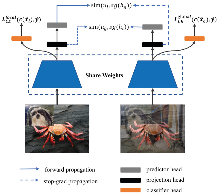
Figure 1. An overview of our GLMC: two types of mixed-label augmented images are processed by an encoder network and a projection head to obtain the representation $h_{g}$ and $h_{l}$ . Then a prediction head transforms the two representations to output $u_{g}$ and $u_{l}$ . We minimize their negative cosine similarity as an auxiliary loss in the supervised loss. $s g(\cdot)$ denotes stop gradient operation.
图 1: 我们的GLMC方法概述:两种混合标签增强图像通过编码器网络和投影头处理,获得表示$h_{g}$和$h_{l}$。随后,预测头将这两个表示转换为输出$u_{g}$和$u_{l}$。我们将它们的负余弦相似度作为监督损失中的辅助损失进行最小化。$sg(\cdot)$表示停止梯度操作。
1. Introduction
1. 引言
Thanks to the available large-scale datasets, e.g., ImageNet [10], MS COCO [27], and Places [46] Database, deep neural networks have achieved dominant results in image recognition [15]. Distinct from these well-designed balanced datasets, data naturally follows long-tail distribution in real-world scenarios, where a small number of head classes occupy most of the samples. In contrast, dominant tail classes only have a few samples. Moreover, the tail classes are critical for some applications, such as medical diagnosis and autonomous driving. Unfortunately, learning directly from long-tailed data may cause model predictions to over-bias toward the head classes.
得益于大规模可用数据集(如ImageNet [10]、MS COCO [27]和Places [46] Database),深度神经网络在图像识别领域取得了主导性成果[15]。与这些精心设计的平衡数据集不同,现实场景中的数据天然遵循长尾分布——少数头部类别占据大多数样本,而占主导地位的尾部类别仅拥有少量样本。此外,尾部类别在某些应用(如医疗诊断和自动驾驶)中至关重要。遗憾的是,直接从长尾数据中学习可能导致模型预测过度偏向头部类别。
There are two classical rebalanced strategies for longtailed distribution, including resampling training data [7, 13, 35] and designing cost-sensitive re weighting loss functions [3, 20]. For the resampling methods, the core idea is to oversample the tail class data or under sample the head classes in the SGD mini-batch to balance training. As for the re weighting strategy, it mainly increases the loss weight of the tail classes to strengthen the tail class. However, learning to rebalance the tail classes directly would damage the original distribution [45] of the long-tailed data, either increasing the risk of over fitting in the tail classes or sacrificing the performance of the head classes. Therefore, these methods usually adopt a two-stage training process [1,3,45] to decouple the representation learning and classifier finetuning: the first stage trains the feature extractor on the original data distribution, then fixes the representation and trains a balanced classifier. Although multi-stage training significantly improves the performance of long-tail recognition, it also negatively increases the training tricks and overhead.
针对长尾分布有两种经典的再平衡策略:重采样训练数据 [7, 13, 35] 和设计成本敏感的重新加权损失函数 [3, 20]。对于重采样方法,其核心思想是在SGD小批量中过采样尾部类别数据或欠采样头部类别数据以实现训练平衡。而重新加权策略则主要通过增加尾部类别的损失权重来强化尾部类别学习。然而,直接学习对尾部类别进行再平衡会破坏长尾数据的原始分布 [45],既可能增加尾部类别过拟合风险,又可能牺牲头部类别的性能。因此,这些方法通常采用两阶段训练流程 [1,3,45] 来解耦表征学习和分类器微调:第一阶段在原始数据分布上训练特征提取器,随后固定表征并训练平衡分类器。尽管多阶段训练显著提升了长尾识别性能,但也负面增加了训练技巧和开销。
In this paper, our goal is to design a simple learning paradigm for long-tail visual recognition, which not only improves the robustness of the feature extractor but also alleviates the bias of the classifier towards head classes while reducing the training skills and overhead. For improving representation robustness, recent contrastive learning techniques [8,18,26,47] that learn the consistency of augmented data pairs have achieved excellence. Still, they typically train the network in a two-stage manner, which does not meet our simplification goals, so we modify them as an auxiliary loss in our supervision loss. For head class bias problems, the typical approach is to initialize a new classifier for resampling or re weighting training. Inspired by the cumulative weighted rebalancing [45] branch strategy, we adopt a more efficient adaptive method to balance the conventional and reweighted classification loss.
本文旨在为长尾视觉识别设计一种简洁的学习范式,该范式既能提升特征提取器的鲁棒性,又可缓解分类器对头部类别的偏置,同时降低训练技巧与开销。为增强表征鲁棒性,近期通过增强数据对一致性进行学习的对比学习技术 [8,18,26,47] 表现优异,但其通常采用两阶段网络训练方式,不符合我们的简化目标,因此我们将其改造为监督损失中的辅助损失项。针对头部类别偏置问题,典型方案是通过初始化新分类器进行重采样或重加权训练。受累积加权重平衡 [45] 分支策略启发,我们采用更高效的自适应方法来平衡常规分类损失与重加权分类损失。
Based on the above analysis, we propose an efficient one-stage training strategy for long-tailed visual recognition called Global and Local Mixture Consistency cumulative learning (GLMC). Our core ideas are twofold: (1) a global and local mixture consistency loss improves the robustness of the model. Specifically, we generate two augmented batches by the global MixUp and local CutMix from the same batch data, respectively, and then use cosine similarity to minimize the difference. (2) A cumulative headtail soft label reweighted loss mitigates the head class bias problem. Specifically, we use empirical class frequencies to reweight the mixed label of the head-tail class for longtailed data and then balance the conventional loss and the rebalanced loss with a coefficient accumulated by epochs.
基于上述分析,我们提出了一种高效的长尾视觉识别单阶段训练策略——全局局部混合一致性累积学习(GLMC)。其核心思想包含两方面:(1) 全局局部混合一致性损失提升模型鲁棒性。具体而言,我们分别通过全局MixUp和局部CutMix从同一批数据生成两个增强批次,然后使用余弦相似度最小化差异。(2) 累积式头尾软标签重加权损失缓解头部类别偏差问题。具体而言,我们使用经验类别频率对长尾数据的头尾类别混合标签进行重加权,然后通过逐轮累积的系数平衡常规损失与重加权损失。
Our method is mainly evaluated in three widely used long-tail image classification benchmark datasets, which include CIFAR10-LT, CIFAR100-LT, and ImageNet-LT datasets. Extensive experiments show that our approach outperforms other methods by a large margin, which verifies the effectiveness of our proposed training scheme. Additional experiments on balanced ImageNet and CIFAR demonstrate that GLMC can significantly improve the genera liz ation of backbones. The main contributions of our work can be summarized as follows:
我们的方法主要在三个广泛使用的长尾图像分类基准数据集上进行评估,包括CIFAR10-LT、CIFAR100-LT和ImageNet-LT数据集。大量实验表明,我们的方法大幅优于其他方法,验证了所提出训练方案的有效性。在平衡的ImageNet和CIFAR上进行的额外实验表明,GLMC能显著提升主干网络的泛化能力。我们工作的主要贡献可总结如下:
• We propose an efficient one-stage training strategy called Global and Local Mixture Consistency cumulative learning framework (GLMC), which can effectively improve the generalization of the backbone for long-tailed visual recognition.
• 我们提出了一种高效的单阶段训练策略,称为全局与局部混合一致性累积学习框架 (GLMC) ,能有效提升主干网络在长尾视觉识别任务中的泛化能力。
• GLMC does not require negative sample pairs or large batches and can be as an auxiliary loss added in supervised loss.
• GLMC 不需要负样本对或大批量数据,可以作为监督损失中的辅助损失。
• Our GLMC achieves state-of-the-art performance on three challenging long-tailed recognition benchmarks, including CIFAR10-LT, CIFAR100-LT, and ImageNet-LT datasets. Moreover, experimental results on full ImageNet and CIFAR validate the effectiveness of GLMC under a balanced setting.
• 我们的GLMC在三个具有挑战性的长尾识别基准测试(CIFAR10-LT、CIFAR100-LT和ImageNet-LT数据集)上实现了最先进的性能。此外,在完整ImageNet和CIFAR上的实验结果验证了GLMC在平衡设置下的有效性。
2. Related Work
2. 相关工作
2.1. Contrastive Representation Learning
2.1. 对比表征学习 (Contrastive Representation Learning)
The recent renaissance of self-supervised learning is expected to obtain a general and transfer r able feature representation by learning pretext tasks. For computer vision, these pretext tasks include rotation prediction [22], relative position prediction of image patches [11], solving jigsaw puzzles [30], and image color iz ation [23, 43]. However, these pretext tasks are usually domain-specific, which limits the generality of learned representations.
自监督学习的近期复兴旨在通过学习代理任务(pretext task)来获取通用且可迁移的特征表示。在计算机视觉领域,这些代理任务包括旋转预测 [22]、图像块相对位置预测 [11]、拼图求解 [30] 以及图像着色 [23, 43]。然而,这些代理任务通常具有领域特定性,从而限制了所学表征的通用性。
Contrastive learning is a significant branch of selfsupervised learning. Its pretext task is to bring two augmented images (seen as positive samples) of one image closer than the negative samples in the representation space. Recent works [17, 31, 36] have attempted to learn the embedding of images by maximizing the mutual information of two views of an image between latent representations. However, their success relies on a large number of negative samples. To handle this issue, BYOL [12] removes the negative samples and directly predicts the output of one view from another with a momentum encoder to avoid collapsing. Instead of using a momentum encoder, Simsiam [5] adopts siamese networks to maximize the cosine similarity between two augmentations of one image with a simple stop-gradient technique to avoid collapsing.
对比学习 (Contrastive Learning) 是自监督学习的重要分支,其前置任务是通过在表征空间中拉近同一图像的两个增强版本(视为正样本)与负样本的距离。近期研究 [17, 31, 36] 尝试通过最大化图像两个视角在潜在表征间的互信息来学习图像嵌入,但这些方法的成功依赖于大量负样本。为解决该问题,BYOL [12] 移除了负样本,直接通过动量编码器从一个视角预测另一个视角的输出以避免坍塌。Simsiam [5] 则采用孪生网络结构,通过简单的停止梯度技术最大化同一图像两种增强版本的余弦相似度,从而避免使用动量编码器。
For long-tail recognition, there have been numerous works [8, 18, 26, 47] to obtain a balanced representation space by introducing a contrastive loss. However, they usually require a multi-stage pipeline and large batches of negative examples for training, which negatively increases training skills and overhead. Our method learns the consistency of the mixed image by cosine similarity, and this method is conveniently added to the supervised training in an auxiliary loss way. Moreover, our approach neither uses negative pairs nor a momentum encoder and does not rely on largebatch training.
针对长尾识别问题,已有大量研究[8, 18, 26, 47]通过引入对比损失来获得平衡的表征空间。然而,这些方法通常需要多阶段流程和大量负样本进行训练,这会显著增加训练难度和开销。我们的方法通过余弦相似度学习混合图像的一致性,并以辅助损失的形式便捷地加入监督训练。此外,我们的方法既不使用负样本对,也不采用动量编码器,且无需依赖大批量训练。
2.2. Class Rebalance learning
2.2. 类别重平衡学习
Rebalance training has been widely studied in long-tail recognition. Its core idea is to strengthen the tail class by oversampling [4, 13] or increasing weight [2, 9, 44]. However, over-learning the tail class will also increase the risk of over fitting [45]. Conversely, under-sampling or reducing weight in the head class will sacrifice the performance of head classes. Recent studies [19, 45] have shown that directly training the rebalancing strategy would degrade the performance of representation extraction, so some multistage training methods [1, 19, 45] decouple the training of representation learning and classifier for long-tail recognition. For representation learning, self-supervised-based [18, 26, 47] and augmentation-based [6, 32] methods can improve robustness to long-tailed distributions. And for the rebalanced classifier, such as multi-experts [24, 37], reweighted class if i ers [1], and label-distribution-aware [3], all can effectively enhance the performance of tail classes. Further, [45] proposed a unified Bilateral-Branch Network (BBN) that adaptively adjusts the conventional learning branch and the reversed sampling branch through a cumulative learning strategy. Moreover, we follow BBN to weight the mixed labels of long-tailed data adaptively and do not require an ensemble during testing.
重平衡训练在长尾识别领域已被广泛研究。其核心思想是通过过采样[4,13]或增加权重[2,9,44]来强化尾部类别。但过度学习尾部类别也会增加过拟合风险[45]。反之,对头部类别进行欠采样或降低权重则会牺牲头部类别的性能。近期研究[19,45]表明,直接采用重平衡策略训练会降低特征提取的表现,因此一些多阶段训练方法[1,19,45]将长尾识别任务解耦为特征学习和分类器训练两个阶段。在特征学习方面,基于自监督[18,26,47]和基于数据增强[6,32]的方法能提升模型对长尾分布的鲁棒性;而在重平衡分类器方面,如多专家系统[24,37]、重加权分类器[1]和标签分布感知方法[3]都能有效提升尾部类别性能。进一步地,[45]提出了统一的双边分支网络(BBN),通过累积学习策略自适应调整常规学习分支和反向采样分支。此外,我们借鉴BBN框架对长尾数据的混合标签进行自适应加权,且无需在测试阶段进行模型集成。
3. The Proposed Method
3. 提出的方法
In this section, we provide a detailed description of our GLMC framework. First, we present an overview of our framework in Sec.3.1. Then, we introduce how to learn global and local mixture consistency by maximizing the cosine similarity of two mixed images in Sec.3.2. Next, we propose a cumulative class-balanced strategy to weight long-tailed data labels progressively in Sec.3.3. Finally, we introduce how to optionally use MaxNorm [1, 16] to finetune the classifier weights in Sec.3.4.
在本节中,我们将详细介绍GLMC框架。首先,在3.1节概述框架结构;其次,在3.2节阐述如何通过最大化两幅混合图像的余弦相似度来学习全局与局部混合一致性;接着,在3.3节提出渐进式加权长尾数据标签的累积类平衡策略;最后,在3.4节说明如何选择性使用MaxNorm [1, 16]微调分类器权重。
3.1. Overall Framework
3.1. 总体框架
Our framework is divided into the following six major components:
我们的框架分为以下六个主要组件:
• A predictor $p r e d(x)$ that maps the output of projection to the contrastive space. The predictor also a fully connected layer and has no activation function. • A linear conventional classifier head $c(x)$ that maps vectors $r$ to category space. The classifier head calculates mixed cross entropy loss with the original data distribution. (optional) A linear rebalanced classifier head $c b(x)$ that maps vectors $r$ to rebalanced category space. The rebalanced classifier calculates mixed cross entropy loss with the reweighted data distribution.
• 一个预测器 $pred(x)$,将投影输出映射到对比空间。该预测器同样是一个全连接层且不含激活函数。
• 一个线性常规分类头 $c(x)$,将向量 $r$ 映射到类别空间。该分类头基于原始数据分布计算混合交叉熵损失。
(可选)一个线性再平衡分类头 $cb(x)$,将向量 $r$ 映射到再平衡类别空间。该再平衡分类器基于重加权数据分布计算混合交叉熵损失。
Note that only the rebalanced classifier $c b(x)$ is retained at the end of training for the long-tailed recognition, while the predictor, projection, and conventional classifier head will be removed. However, for the balanced dataset, the rebalanced classifier $c b(x)$ is not needed.
请注意,在长尾识别的训练结束时,仅保留重新平衡的分类器 $c b(x)$,而预测器、投影层和常规分类器头部将被移除。然而,对于平衡数据集,则不需要重新平衡的分类器 $c b(x)$。
3.2. Global and Local Mixture Consistency Learning
3.2. 全局与局部混合一致性学习
In supervised deep learning, the model is usually divided into two parts: an encoder and a linear classifier. And the class if i ers are label-biased and rely heavily on the quality of representations. Therefore, improving the generalization ability of the encoder will significantly improve the fi- nal classification accuracy of the long-tailed challenge. Inspired by self-supervised learning to improve representation by learning additional pretext tasks, as illustrated in Fig.1, we train the encoder using a standard supervised task and a self-supervised task in a multi-task learning way. Further, unlike simple pretext tasks such as rotation prediction, image color iz ation, etc., following the global and local ideas [39], we expect to learn the global-local consistency through the strong data augmentation method MixUp [42] and CutMix [41].
在监督式深度学习中,模型通常分为两部分:编码器和线性分类器。而分类器存在标签偏差,高度依赖表征质量。因此,提升编码器的泛化能力将显著改善长尾挑战的最终分类准确率。受自监督学习通过额外代理任务提升表征的启发(如图1所示),我们采用多任务学习方式,同时用标准监督任务和自监督任务训练编码器。此外,不同于旋转预测、图像着色等简单代理任务,遵循全局-局部思想[39],我们期望通过MixUp[42]和CutMix[41]这类强数据增强方法学习全局-局部一致性。
Global Mixture. MixUp is a global mixed-label data augmentation method that generates mixture samples by mixing two images of different classes. For a pair of two images and their labels probabilities $\left({x_{i},p_{i}}\right)$ and $(x_{j},p_{j})$ , we calculate $(\tilde{x}{g},\tilde{p}_{g})$ by
全局混合 (Global Mixture)。MixUp 是一种全局混合标签的数据增强方法,通过混合两张不同类别的图像生成混合样本。对于一对图像及其标签概率 $\left({x_{i},p_{i}}\right)$ 和 $(x_{j},p_{j})$,我们通过以下公式计算 $(\tilde{x}{g},\tilde{p}_{g})$:
$$
\begin{array}{c}{{\lambda\sim B e t a(\beta,\beta),}}\ {{\tilde{x}{g}=\lambda x_{i}+(1-\lambda)x_{j},}}\ {{\tilde{p}{g}=\lambda p_{i}+(1-\lambda)p_{j}.}}\end{array}
$$
$$
\begin{array}{c}{{\lambda\sim B e t a(\beta,\beta),}}\ {{\tilde{x}{g}=\lambda x_{i}+(1-\lambda)x_{j},}}\ {{\tilde{p}{g}=\lambda p_{i}+(1-\lambda)p_{j}.}}\end{array}
$$
where $\lambda$ is sampled from a Beta distribution parameterized by the $\beta$ hyper-parameter. Note that $p$ are one-hot vectors. Local Mixture. Different from MixUp, CutMix combines two images by locally replacing the image region with a patch from another training image. We define the combining operation as
其中 $\lambda$ 是从由超参数 $\beta$ 参数化的 Beta 分布中采样得到的。注意 $p$ 是独热(one-hot)向量。局部混合(Local Mixture)。与 MixUp 不同,CutMix 通过用另一张训练图像的局部区域替换当前图像的局部区域来组合两张图像。我们将这种组合操作定义为
$$
\tilde{x}{l}=M\odot x_{i}+({\bf1}-M)\odot x_{j}.
$$
$$
\tilde{x}{l}=M\odot x_{i}+({\bf1}-M)\odot x_{j}.
$$
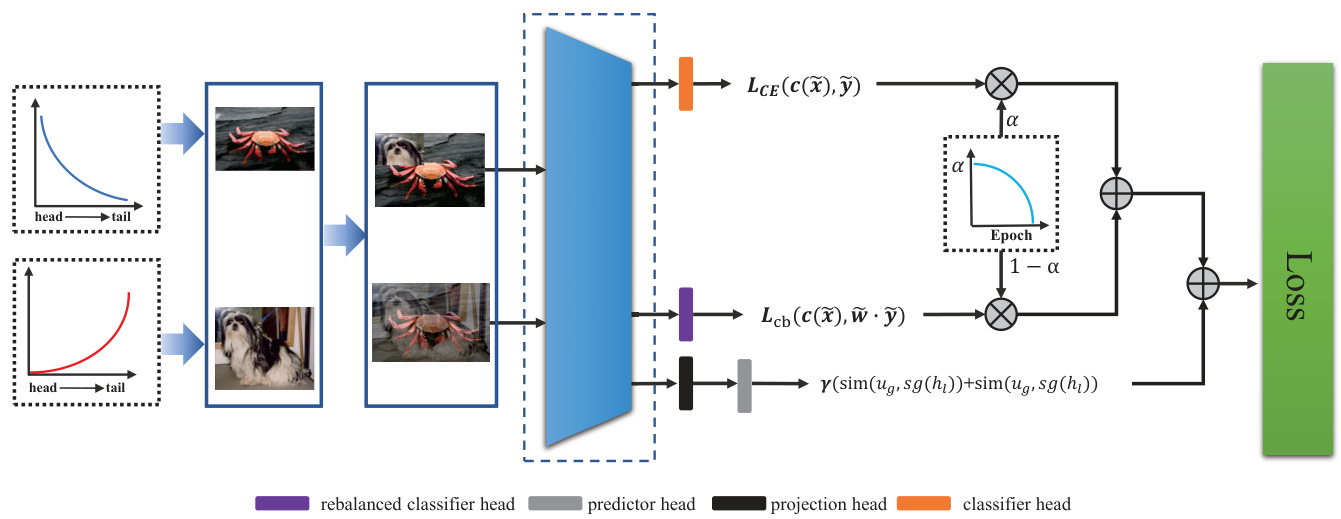
Figure 2. An illustration of the cumulative class-balanced learning pipeline. We apply uniform and reversed samplers to obtain head and tail data, and then they are synthesized into head-tail mixture samples by MixUp and CutMix. The cumulative learning strategy adaptively weights the rebalanced classifier and the conventional classifier by epochs.
图 2: 累积式类别平衡学习流程示意图。我们采用均匀采样器和反向采样器分别获取头部数据和尾部数据,随后通过 MixUp 和 CutMix 将其合成为头尾混合样本。累积学习策略根据训练周期自适应地加权平衡分类器与常规分类器。
where $M\in{0,1}^{W\times H}$ denotes the randomly selected pixel patch from the image $x_{i}$ and pasted on $x_{j}$ , 1 is a binary mask filled with ones, and $\odot$ is element-wise multiplication. Concretely, we sample the bounding box coordinates $\boldsymbol{B}=\left(r_{x},r_{y},r_{w},r_{h}\right)$ indicating the cropping regions on $x_{i}$ and $x_{j}$ . The box coordinates are uniformly sampled according to
其中 $M\in{0,1}^{W\times H}$ 表示从图像 $x_{i}$ 中随机选取并粘贴到 $x_{j}$ 上的像素块,1 是填充为全1的二元掩码,$\odot$ 表示逐元素相乘。具体而言,我们采样边界框坐标 $\boldsymbol{B}=\left(r_{x},r_{y},r_{w},r_{h}\right)$ 来指示 $x_{i}$ 和 $x_{j}$ 上的裁剪区域。这些框坐标是根据均匀分布采样的。
$$
\begin{array}{l l}{{r_{x}\sim U n i f o r m(0,W),r_{w}=W\sqrt{1-\lambda}}}\ {{r_{y}\sim U n i f o r m(0,H),r_{h}=H\sqrt{1-\lambda}}}\end{array}
$$
$$
\begin{array}{l l}{{r_{x}\sim U n i f o r m(0,W),r_{w}=W\sqrt{1-\lambda}}}\ {{r_{y}\sim U n i f o r m(0,H),r_{h}=H\sqrt{1-\lambda}}}\end{array}
$$
where $\lambda$ is also sampled from the $B e t a(\beta,\beta)$ , and their mixed labels are the same as MixUp.
其中 $\lambda$ 也采样自 $B e t a(\beta,\beta)$ ,混合标签与 MixUp 相同。
Self-Supervised Learning Branch. Previous works require large batches of negative samples [17, 36] or a memory bank [14] to train the network. That makes it difficult to apply to devices with limited memory. For simplicity, our goal is to maximize the cosine similarity of global and local mixtures in representation space to obtain contrastive consistency. Specifically, the two types of augmented images are processed by an encoder network and a projection head to obtain the representation $h_{g}$ and $h_{l}$ . Then a prediction head transforms the two representations to output $u_{g}$ and $u_{l}$ . We minimize their negative cosine similarity:
自监督学习分支。先前的研究需要大批量负样本 [17, 36] 或记忆库 [14] 来训练网络,这使其难以应用于内存受限的设备。为简化流程,我们的目标是通过最大化全局与局部混合特征在表征空间中的余弦相似度来获得对比一致性。具体而言,两种增强图像经过编码器网络和投影头处理后得到表征 $h_{g}$ 和 $h_{l}$,随后预测头将这两个表征转换为输出 $u_{g}$ 和 $u_{l}$。我们通过最小化它们的负余弦相似度来实现优化:
$$
s i m(u_{g},h_{l})=-\frac{u_{g}}{|u_{g}|}\cdot\frac{h_{l}}{|h_{l}|}
$$
$$
s i m(u_{g},h_{l})=-\frac{u_{g}}{|u_{g}|}\cdot\frac{h_{l}}{|h_{l}|}
$$
where $\left\Vert\cdot\right\Vert$ is $l_{2}$ normalization. An undesired trivial solution to minimize the negative cosine similarity of augmented images is all outputs “collapsing” to a constant. Following SimSiam [5], we use a stop gradient operation to prevent collapsing. The SimSiam loss function is defined as:
其中 $\left\Vert\cdot\right\Vert$ 表示 $l_{2}$ 归一化。最小化增强图像负余弦相似度时可能出现所有输出"坍缩"为常数的平凡解。借鉴 SimSiam [5] 的方法,我们采用停止梯度操作防止坍缩,其损失函数定义为:
$$
\mathcal{L}{s i m}=s i m(u_{g},s g(h_{l}))+s i m(u_{l},s g(h_{g}))
$$
$$
\mathcal{L}{s i m}=s i m(u_{g},s g(h_{l}))+s i m(u_{l},s g(h_{g}))
$$
this means that $h_{l}$ and $h_{g}$ are treated as a constant.
这意味着 $h_{l}$ 和 $h_{g}$ 被视为常量。
Supervised Learning Branch. After constructing the global and local augmented data pair $(\tilde{x}{g};\tilde{p}{g})$ and $(\tilde{x}{l};\tilde{p}_{l})$ , we calculate the mixed-label cross-entropy loss:
监督学习分支。在构建全局和局部增强数据对 $(\tilde{x}{g};\tilde{p}{g})$ 和 $(\tilde{x}{l};\tilde{p}_{l})$ 后,我们计算混合标签交叉熵损失:
$$
\mathcal{L}{c}=-\frac{1}{2N}\sum_{i=1}^{N}(\tilde{p}{g}^{i}(l o g f(\tilde{x}{g}^{i}))+\tilde{p}{l}^{i}(l o g f(\tilde{x}_{l}^{i})))
$$
$$
\mathcal{L}{c}=-\frac{1}{2N}\sum_{i=1}^{N}(\tilde{p}{g}^{i}(l o g f(\tilde{x}{g}^{i}))+\tilde{p}{l}^{i}(l o g f(\tilde{x}_{l}^{i})))
$$
where $N$ denote the sampling batch size and $f(\cdot)$ denote predicted probability of $\tilde{x}$ . Note that a batch of images is augmented into a global and local mixture so that the actual batch size will be twice the sampling size.
其中 $N$ 表示采样批次大小,$f(\cdot)$ 表示 $\tilde{x}$ 的预测概率。需要注意的是,图像批次会被增强为全局和局部混合形式,因此实际批次大小将是采样大小的两倍。
3.3. Cumulative Class-Balanced Learning
3.3. 累积式类别平衡学习
Class-Balanced learning. The design principle of class re weighting is to introduce a weighting factor inversely proportional to the label frequency and then strengthen the learning of the minority class. Following [44], the weighting factor $w_{i}$ is define as:
类别平衡学习。类别重新加权的设计原则是引入一个与标签频率成反比的权重因子,从而加强对少数类别的学习。根据[44],权重因子$w_{i}$定义为:
$$
w_{i}={\frac{C\cdot(1/r_{i})^{k}}{\sum_{i=1}^{C}(1/r_{i})^{k}}}
$$
$$
w_{i}={\frac{C\cdot(1/r_{i})^{k}}{\sum_{i=1}^{C}(1/r_{i})^{k}}}
$$
where $r_{i}$ is the i-th class frequencies of the training dataset, and $k$ is a hyper-parameter to scale the gap between the head and tail classes. Note that $k=0$ corresponds to no reweighting and $k=1$ corresponds to class-balanced method [9]. We change the scalar weights to the one-hot vectors form and mix the weight vectors of the two images:
其中 $r_{i}$ 表示训练数据集中第i类的频率,$k$ 是用于调节头部与尾部类别差距的超参数。注意 $k=0$ 表示不进行重新加权,$k=1$ 对应类别平衡方法 [9]。我们将标量权重转换为独热向量形式,并混合两幅图像的权重向量:
$$
\tilde{w}=\lambda w_{i}+(1-\lambda)w_{j}.
$$
$$
\tilde{w}=\lambda w_{i}+(1-\lambda)w_{j}.
$$
Formally, given a train dataset $D={(x_{i},y_{i},w_{i})}_{i=1}^{N}$ , the rebalanced loss can be written as:
给定训练数据集 $D={(x_{i},y_{i},w_{i})}_{i=1}^{N}$ ,重平衡损失可表示为:
$$
\mathcal{L}{c b}=-\frac{1}{2N}\sum_{i=1}^{N}\tilde{w}^{i}(\tilde{p}{g}^{i}(l o g f(\tilde{x}{g}^{i}))+\tilde{p}{l}^{i}(l o g f(\tilde{x}_{l}^{i})))
$$
$$
\mathcal{L}{c b}=-\frac{1}{2N}\sum_{i=1}^{N}\tilde{w}^{i}(\tilde{p}{g}^{i}(l o g f(\tilde{x}{g}^{i}))+\tilde{p}{l}^{i}(l o g f(\tilde{x}_{l}^{i})))
$$
Table 1. Top-1 accuracy $(%)$ of ResNet-32 on CIFAR-10-LT and CIFAR-100-LT with different imbalance factors [100, 50, 10]. GLMC consistently outperformed the previous best method only in the one-stage.
表 1. ResNet-32 在 CIFAR-10-LT 和 CIFAR-100-LT 上不同不平衡因子 [100, 50, 10] 的 Top-1 准确率 $(%)$。GLMC 仅在单阶段训练中持续优于先前的最佳方法。
| 方法 | CIFAR-10-LT | CIFAR-100-LT | |||||
|---|---|---|---|---|---|---|---|
| IF=100 | 50 | 10 | 100 | 50 | 10 | ||
| CE | 70.4 | 74.8 | 86.4 | 38.3 | 43.9 | 55.7 | |
| 重平衡分类器 | BBN [45] | 79.82 | 82.18 | 88.32 | 42.56 | 47.02 | 59.12 |
| CB-Focal [9] | 74.6 | 79.3 | 87.1 | 39.6 | 45.2 | 58 | |
| LogitAjust [29] | 80.92 | 42.01 | 47.03 | 57.74 | |||
| weight balancing [1] | 53.35 | 57.71 | 68.67 | ||||
| 数据增强 | Mixup [42] | 73.06 | 77.82 | 87.1 | 39.54 | 54.99 | 58.02 |
| RISDA [6] | 79.89 | 79.89 | 79.89 | 50.16 | 53.84 | 62.38 | |
| CMO [32] | 47.2 | 51.7 | 58.4 | ||||
| 自监督预训练 | KCL [18] | 77.6 | 81.7 | 88 | 42.8 | 46.3 | 57.6 |
| TSC [25] | 79.7 | 82.9 | 88.7 | 42.8 | 46.3 | 57.6 | |
| BCL [47] | 84.32 | 87.24 | 91.12 | 51.93 | 56.59 | 64.87 | |
| PaCo [8] | 52 | 56 | 64.2 | ||||
| SSD [26] | 46 | 50.5 | 62.3 | ||||
| 集成分类器 | RIDE (3 experts) + CMO [32] | 50 | 53 | 60.2 | |||
| RIDE (3 experts) [37] | 48.6 | 51.4 | 59.8 | ||||
| 单阶段训练 | ours | 87.75 | 90.18 | 94.04 | 55.88 | 61.08 | 70.74 |
| 微调分类器 | ours + MaxNorm [1] | 87.57 | 90.22 | 94.03 | 57.11 | 62.32 | 72.33 |
where $f(\tilde{x})$ and $\tilde{w}$ denote predicted probability and weighting factor of mixed image $\tilde{x}$ , respectively. Note that the global and local mixed image have the same mixed weights.
其中 $f(\tilde{x})$ 和 $\tilde{w}$ 分别表示混合图像 $\tilde{x}$ 的预测概率和权重因子。注意全局和局部混合图像具有相同的混合权重。
Cumulative Class-Balanced Learning. As illustrated in Fig.2, we use the bilateral branches structure to learn the rebalance branch adaptively. But unlike BBN [45], our cumulative learning strategy is imposed on the loss function instead of the fully connected layer weights and uses re weighting instead of resampling for learning. Concretely, the loss $\mathcal{L}{c}$ of the unweighted classification branch is multiplied by $\alpha$ , and the rebalanced loss $\mathcal{L}_{c b}$ is multiplied by $1-\alpha$ . $\alpha$ automatically decreases as the current training epochs $T$ increase:
累积类别平衡学习。如图 2 所示,我们使用双边分支结构自适应地学习重平衡分支。但与 BBN [45] 不同,我们的累积学习策略施加于损失函数而非全连接层权重,并采用重加权 (reweighting) 而非重采样 (resampling) 进行学习。具体而言,未加权分类分支的损失 $\mathcal{L}{c}$ 乘以 $\alpha$,重平衡损失 $\mathcal{L}_{c b}$ 乘以 $1-\alpha$。$\alpha$ 会随着当前训练周期 $T$ 的增加而自动递减:
$$
\alpha=1-(\frac{T}{T_{m a x}})^{2}
$$
$$
\alpha=1-(\frac{T}{T_{m a x}})^{2}
$$
where $T_{m a x}$ is the maximum training epoch.
其中 $T_{m a x}$ 为最大训练轮次。
Finally, the total loss is defined as a combination of loss $L_{s u p},L_{c b}$ , and $L_{s i m}$ :
最终,总损失定义为损失 $L_{s u p},L_{c b}$ 和 $L_{s i m}$ 的组合:
$$
\mathcal{L}{t o t a l}=\alpha\mathcal{L}{c}+(1-\alpha)\mathcal{L}{c b}+\gamma\mathcal{L}_{s i m}
$$
$$
\mathcal{L}{t o t a l}=\alpha\mathcal{L}{c}+(1-\alpha)\mathcal{L}{c b}+\gamma\mathcal{L}_{s i m}
$$
where $\gamma$ is a hyper parameter that controls $L_{s i m}$ loss. The default value is 10.
其中 $\gamma$ 是控制 $L_{s i m}$ 损失的超参数,默认值为10。
3.4. Finetuning Classifier Weights
3.4. 微调分类器权重
[1] investigate that the classifier weights would be heavily biased toward the head classes when faced with longtail data. Therefore, we optionally use MaxNorm [1, 16]
[1] 研究发现,分类器权重在面对长尾数据时会严重偏向头部类别。因此,我们可选地采用 MaxNorm [1, 16]
to finetune the classifier in the second stage. Specifically, MaxNorm restricts weight norms within a ball of radius $\delta$ :
在第二阶段微调分类器。具体而言,MaxNorm将权重范数限制在半径为$\delta$的球体内:
$$
\Theta^{\ast}=a r g m i n F(\Theta;D),s.t.||\theta_{k}||_{2}^{2}\leq\delta^{2}
$$
$$
\Theta^{\ast}=a r g m i n F(\Theta;D),s.t.||\theta_{k}||_{2}^{2}\leq\delta^{2}
$$
this can be solved by applying projected gradient descent (PGD). For each epoch (or iteration), PGD first computes an updated $\theta_{k}$ and then projects it onto the norm ball:
这可以通过应用投影梯度下降 (PGD) 来解决。对于每个周期 (或迭代),PGD 首先计算更新后的 $\theta_{k}$,然后将其投影到范数球上:
$$
\theta_{k}\gets m i n(1,\delta/||\theta_{k}||{2})*\theta_{k}
$$
$$
\theta_{k}\gets m i n(1,\delta/||\theta_{k}||{2})*\theta_{k}
$$
4. Experiments
4. 实验
In this section, we evaluate the proposed GLMC on three widely used long-tailed benchmarks: CIFAR-10-LT, CIFAR-100-LT, and ImageNet-LT. We also conduct a series of ablation studies to assess each component of GLMC’s importance fully.
在本节中,我们在三个广泛使用的长尾基准数据集(CIFAR-10-LT、CIFAR-100-LT和ImageNet-LT)上评估了提出的GLMC方法。同时通过一系列消融实验全面分析了GLMC各组件的重要性。
4.1. Experiment setup
4.1. 实验设置
Datasets. Following [40], we modify the balanced CIFAR10, CIFAR100, and ImageNet-2012 dataset to the uneven setting (named CIFAR10-LT, CIFAR100-LT, and ImageNet-LT) by utilizing the exponential decay function $n=n_{i}\mu^{i}$ , where $i$ is the class index (0-indexed), $n_{i}$ is the original number of training images and $\mu\in(0,1)$ . The imbalanced factor $\beta$ is defined by $\beta=N_{m a x}/N_{m i n}$ , which reflects the degree of imbalance in the data. CIFAR10- LT and CIFAR100-LT are divided into three types of train datasets, and each dataset has a different imbalance factor [100,50,10]. ImageNet-LT has a 256 imbalance factor. The most frequent class includes 1280 samples, while the least contains only 5.
数据集。遵循[40]的做法,我们通过指数衰减函数$n=n_{i}\mu^{i}$将平衡的CIFAR10、CIFAR100和ImageNet-2012数据集调整为非均衡设置(分别命名为CIFAR10-LT、CIFAR100-LT和ImageNet-LT),其中$i$为类别索引(从0开始),$n_{i}$为原始训练图像数量,$\mu\in(0,1)$。不平衡因子$\beta$由$\beta=N_{max}/N_{min}$定义,反映数据的不平衡程度。CIFAR10-LT和CIFAR100-LT被划分为三种训练数据集类型,每种数据集具有不同的不平衡因子[100,50,10]。ImageNet-LT的不平衡因子为256,最频繁类别包含1280个样本,而最少类别仅含5个样本。
Table 2. Top-1 accuracy $(%)$ on ImageNet-LT dataset. Comparison to the state-of-the-art methods with different backbone. $^\dagger$ denotes results reproduced by [47] with 180 epochs.
表 2: ImageNet-LT 数据集上的 Top-1 准确率 $(%)$ 。与不同骨干网络的最新方法对比。$^\dagger$ 表示由 [47] 复现的 180 轮次结果。
| 方法 | 骨干网络 | ImageNet-LT | |||
|---|---|---|---|---|---|
| Many | Med | Few | All | ||
| CE | ResNet-50 | 64 | 33.8 | 5.8 | 41.6 |
| CB-Focal [9] | ResNet-50 | 39.6 | 32.7 | 16.8 | 33.2 |
| LDAM [3] | ResNet-50 | 60.4 | 46.9 | 30.7 | 49.8 |
| KCL [18] | ResNet-50 | 61.8 | 49.4 | 30.9 | 51.5 |
| TSC [25] | ResNet-50 | 63.5 | 49.7 | 30.4 | 52.4 |
| RISDA [6] | ResNet-50 | - | - | - | 49.3 |
| BCL (90 epochs) [47] | ResNeXt-50 | 67.2 | 53.9 | 36.5 | 56.7 |
| BCL (180 epochs) [47] | ResNeXt-50 | 67.9 | 54.2 | 36.6 | 57.1 |
| PaCot (180 epochs) [8] | ResNeXt-50 | 64.4 | 55.7 | 33.7 | 56.0 |
| Balanced Softmax (180 epochs) [34] | ResNeXt-50 | 65.8 | 53.2 | 34.1 | 55.4 |
| SSD [26] | ResNeXt-50 | 66.8 | 53.1 | 35.4 | 56 |
| RIDE (3 experts) + CMO [32] | ResNet-50 | 66.4 | 53.9 | 35.6 | 56.2 |
| RIDE (3 experts) [37] | Swin-S | 66.9 | 52.8 | 37.4 | 56 |
| weight balancing + MaxNorm [1] | ResNeXt-50 | 62.5 | 50.4 | 41.5 | 53.9 |
| ours | - | 70.1 | 52.4 | 30.4 | 56.3 |
| ours + MaxNorm [1] | ResNeXt-50 | 60.8 | 55.9 | 45.5 | 56.7 |
| ours + BS [34] | - | 64.76 | 55.67 | 42.19 | 57.21 |
Network architectures. For a fair comparison with recent works, we follow [1, 8, 47] to use ResNet-32 [15] on CIFAR10-LT and CIFAR100-LT, ResNet-50 [15] and $\mathrm{ResNeXt}.50.32\mathrm{x}4\mathrm{d}$ [38] on ImageNet-LT. The main ablation experiment was performed using ResNet-32 on the CIFAR100 dataset.
网络架构。为了与近期工作进行公平比较,我们遵循[1, 8, 47]的研究方案:在CIFAR10-LT和CIFAR100-LT上使用ResNet-32[15],在ImageNet-LT上使用ResNet-50[15]和$\mathrm{ResNeXt}.50.32\mathrm{x}4\mathrm{d}$[38]。主要消融实验采用CIFAR100数据集上的ResNet-32完成。
Evaluation protocol. For each dataset, we train them on the imbalanced training set and evaluate them in the balanced validation/test set. Following [1, 28], we further report accuracy on three splits of classes, Many-shot classes (training samples $ >100 $ ), Medium-shot (training samples $20 \sim100 $ ) and Few-shot (training samples $ \leq20 $ ), to compre hens iv ely evaluate our model.
评估协议。对于每个数据集,我们在不平衡的训练集上进行训练,并在平衡的验证/测试集上进行评估。遵循 [1, 28] 的方法,我们进一步报告三类样本的准确率:多样本类(训练样本 $ >100$)、中等样本类(训练样本 $20 \sim100 $)和少样本类(训练样本 $ \leq20 $),以全面评估模型性能。
Implementation. We train our models using the PyTorch toolbox [33] on GeForce RTX 3090 GPUs. All models are implemented by the SGD optimizer with a momen- tum of 0.9 and gradually decay learning rate with a cosine annealing scheduler, and the batch size is 128. For CIFAR10-LT and CIFAR100-LT, the initial learning rate is 0.01, and the weight decay rate is 5e-3. For ImageNet-LT, the initial learning rate is 0.1, and the weight decay rate is 2e-4. We also use random horizontal flipping and cropping as simple augmentation.
实现。我们使用PyTorch工具箱[33]在GeForce RTX 3090 GPU上训练模型。所有模型均采用SGD优化器实现,动量为0.9,并通过余弦退火调度器逐步衰减学习率,批量大小为128。对于CIFAR10-LT和CIFAR100-LT,初始学习率为0.01,权重衰减率为5e-3;对于ImageNet-LT,初始学习率为0.1,权重衰减率为2e-4。我们还采用随机水平翻转和裁剪作为简单数据增强。
4.2. Long-tailed Benchmark Results
4.2. 长尾基准测试结果
Compared Methods. Since the field of LTR is developing rapidly and has many branches, we choose recently published representative methods of different types for comparison. For example, SSD [26], PaCo [8], KCL [18], BCL [47], and TSC [25] use contrastive learning or selfsupervised methods to train balanced representations. RIDE [37] combines multiple experts for prediction; RISDA [6] and CMO [32] apply strong data augmentation techniques to improve robustness; Weight Balancing [1] is a typical two-stage training method.
对比方法。由于LTR领域发展迅速且分支众多,我们选取近期发表的不同类型代表性方法进行比较。例如,SSD [26]、PaCo [8]、KCL [18]、BCL [47] 和 TSC [25] 采用对比学习或自监督方法训练平衡表征;RIDE [37] 通过组合多个专家模型进行预测;RISDA [6] 和 CMO [32] 应用强数据增强技术提升鲁棒性;Weight Balancing [1] 是典型的两阶段训练方法。
Table 3. Top-1 accuracy $(%)$ on full ImageNet dataset with ResNet-50 backbone.
表 3: 基于ResNet-50骨干网络在完整ImageNet数据集上的Top-1准确率(%)
| 方法 | 数据增强 | Top-1准确率 |
|---|---|---|
| vanilla | Simple Augment | 76.4 |
| vanilla | MixUp [42] | 77.9 |
| vanilla | CutMix [41] | 78.6 |
| Supcon [21] | RandAugment | 78.4 |
| PaCo [8] | Simple Augment | 78.7 |
| PaCo [8] | RandAugment | 79.3 |
| ours | MixUp+CutMix | 80.2 |
Results on CIFAR10-LT and CIFAR100-LT. We conduct extensive experiments to compare GLMC with state-ofthe-art baselines on long-tailed CIFAR10 and CIFAR100 datasets by setting three imbalanced ratios: 10, 50, and 100. Table 1 reports the Top-1 accuracy of various methods on CIFAR-10-LT and CIFAR-100-LT. We can see that our GLMC consistently achieves the best results on all datasets, whether using one-stage training or a two-stage finetune classifier. For example, on CIFAR100-LT $(\mathrm{IF}{=}100)\$ ), Our method achieves $55.88%$ in the first stage, outperforming
CIFAR10-LT 和 CIFAR100-LT 上的结果。我们通过设置 10、50 和 100 三种不平衡比例,在长尾 CIFAR10 和 CIFAR100 数据集上进行了大量实验,将 GLMC 与最先进的基线方法进行比较。表 1 报告了各种方法在 CIFAR-10-LT 和 CIFAR-100-LT 上的 Top-1 准确率。可以看出,无论是使用单阶段训练还是两阶段微调分类器,我们的 GLMC 在所有数据集上始终取得最佳结果。例如,在 CIFAR100-LT $( \mathrm{IF}=100 )$ 上,我们的方法在第一阶段达到了 $55.88%$,优于
Algorithm 1 Learning algorithm of our proposed GLMC
算法 1: 我们提出的GLMC学习算法
Input: Training Dataset $D={(x_{i},y_{i},w_{i})}_{i=1}^{N}$
训练数据集 $D={(x_{i},y_{i},w_{i})}_{i=1}^{N}$
Parameter: $E n c o d e r(\cdot)$ denotes feature extractor; $p r o j(\cdot)$ and $p r e d(\cdot)$ denote projection and predictor; $c(\cdot)$ and $c b(\cdot)$ denote convention classifier and rebalanced classifier; $T_{m a x}$ is the Maximum training epoch; $s g(\cdot)$ denotes stop gradient operation.
参数:$Encoder(\cdot)$ 表示特征提取器;$proj(\cdot)$ 和 $pred(\cdot)$ 分别表示投影器和预测器;$c(\cdot)$ 和 $cb(\cdot)$ 表示常规分类器和平衡分类器;$T_{max}$ 为最大训练周期;$sg(\cdot)$ 表示停止梯度操作。
the two-stage weight rebalancing strategy $(53.35%)$ . After finetuning the classifier with MaxNorm, our method achieves $57.11%$ , which accuracy increased by $+3.76%$ compared with the previous SOTA. Compared to contrastive learning families, such as $\mathrm{PaCo}$ and BCL, GLMC surpasses previous SOTA by $+5.11%$ , $+5.73%$ , and $+7.46%$ under imbalance factors of 100, 50, and 10, respectively. In addition, GLMC does not need a large batch size and long training epoch to pretrain the feature extractor, which reduces training skills.
两阶段权重再平衡策略 $(53.35%)$。使用MaxNorm微调分类器后,我们的方法达到 $57.11%$,准确率较之前的最先进水平(SOTA)提升 $+3.76%$。与对比学习系列方法(如 $\mathrm{PaCo}$ 和BCL)相比,GLMC在100、50和10的不平衡因子下分别以 $+5.11%$、$+5.73%$ 和 $+7.46%$ 超越先前SOTA。此外,GLMC无需大批次量和长训练周期来预训练特征提取器,从而降低了训练技巧要求。
Results on ImageNet-LT. Table 2 compares GLMC with state-of-the-art baselines on ImageNet-LT dataset. We report the Top-1 accuracy on Many-shot, Medium-shot, and Few-shot groups. As shown in the table, with only onestage training, GLMC significantly improves the performance of the head class by $70.1%$ , and the overall performance reaches $56.3%$ , similar to $\mathrm{PaCo}$ (180 epochs). After finetuning the classifier, the tail class of GLMC can reach $45.5%$ ( $^+$ MaxNorm [1]) and $42.19%$ $(+\mathrm{ B S~}$ [34]), which significantly improves the performance of the tail class.
ImageNet-LT上的结果。表2比较了GLMC与ImageNet-LT数据集上最先进基线的表现。我们报告了多样本、中样本和少样本组的Top-1准确率。如表所示,仅通过单阶段训练,GLMC就将头部类别的性能显著提升至$70.1%$,整体性能达到$56.3%$,与$\mathrm{PaCo}$(180轮训练)相当。在对分类器进行微调后,GLMC的尾部类别准确率可达到$45.5%$($^+$ MaxNorm [1])和$42.19%$($+\mathrm{ B S~}$ [34]),显著提升了尾部类别的性能。
Table 4. Top-1 accuracy $(%)$ on full CIFAR-10 and CIFAR-100 dataset with ResNet-50 backbone.
表 4: 使用 ResNet-50 骨干网络在完整 CIFAR-10 和 CIFAR-100 数据集上的 Top-1 准确率 $(%)$
| 方法 | CIFAR-10 | CIFAR-100 |
|---|---|---|
| vanilla | 94.85 | 75.28 |
| MixUp [42] | 95.95 | 77.99 |
| CutMix [41] | 95.41 | 78.03 |
| SupCon [21] | 96 | 76.5 |
| PaCo [8] | - | 79.1 |
| ours | 97.23 | 83.05 |
4.3. Full ImageNet and CIFAR Recognition
4.3. 完整ImageNet与CIFAR识别
GLMC utilizes a global and local mixture consistency loss as an auxiliary loss in supervised loss to improve the robustness of the model, which can be added to the model as a plug-and-play component. To verify the effectiveness of GLMC under a balanced setting, we conduct experiments on full ImageNet and full CIFAR. They are indicative to compare GLMC with the related state-of-the-art methods (MixUp [42], CutMix [41], PaCo [8], and SupCon [8]). Note that under full ImageNet and CIFAR, we remove the cumulative re weighting and resampling strategies customized for long-tail tasks.
GLMC采用全局与局部混合一致性损失作为监督损失的辅助损失,以提升模型鲁棒性,该组件可作为即插即用模块集成到模型中。为验证GLMC在平衡场景下的有效性,我们在完整ImageNet和CIFAR数据集上进行实验,结果表明GLMC相比当前最先进方法(MixUp [42]、CutMix [41]、PaCo [8]和SupCon [8])具有优势。需注意的是,在完整ImageNet和CIFAR实验中,我们移除了专为长尾任务设计的累积重加权和重采样策略。
Results on Full CIFAR-10 and CIFAR-100. For CIFAR10 and CIFAR-100 implementation, following PaCo and SupCon, we use ResNet-50 as the backbone. As shown in Table 4, on CIFAR-100, GLMC achieves $83.05%$ Top1 accuracy, which outperforms PaCo by $3.95%$ . Furthermore, GLMC exceeds the vanilla cross entropy method by $2.13%$ and $7.77%$ on CIFAR-10 and CIFAR-100, respectively, which can significantly improve the performance of the base model.
完整CIFAR-10与CIFAR-100实验结果。在CIFAR-10和CIFAR-100实验中,我们遵循PaCo和SupCon的方案,采用ResNet-50作为主干网络。如表4所示,在CIFAR-100上,GLMC以83.05%的Top1准确率超越PaCo达3.95%。此外,GLMC在CIFAR-10和CIFAR-100上分别较原始交叉熵方法提升2.13%和7.77%,显著提升了基础模型的性能。
Results on Full ImageNet. In the implementation, we transfer hyper parameters of GLMC on ImageNet-LT to full ImageNet without modification. The experimental results are summarized in Table 3. Our model achieves $80.2%$ Top-1 accuracy, outperforming $\mathrm{PaCo}$ and SupCon by $+0.9%$ and $+1.8%$ , respectively. Compared to the positive/negative contrastive model (PaCo and SupCon). GLMC does not need to construct negative samples, which can effectively reduce memory usage during training.
完整ImageNet上的结果。在实现过程中,我们将GLMC在ImageNet-LT上的超参数直接迁移至完整ImageNet数据集且未作修改。实验结果汇总于表3:我们的模型取得了80.2%的Top-1准确率,分别以+0.9%和+1.8%的优势超越PaCo与SupCon。相较于正负样本对比模型(PaCo和SupCon),GLMC无需构建负样本,能有效降低训练过程中的内存消耗。
4.4. Ablation Study
4.4. 消融实验
To further analyze the proposed GLMC, we perform several ablation studies to evaluate the contribution of each component more comprehensively. All experiments are performed on CIFAR-100 with an imbalance factor of 100.
为进一步分析所提出的GLMC方法,我们进行了多项消融实验,以更全面地评估各组件的贡献。所有实验均在CIFAR-100数据集上进行,不平衡因子设为100。

Figure 3. Confusion matrices of different label re weighting and resample coefficient $k$ on CIFAR-100-LT with an imbalance ratio of 100.
图 3: 不同标签重加权和重采样系数 $k$ 在失衡比为 100 的 CIFAR-100-LT 数据集上的混淆矩阵。
The effect of rebalancing intensity. As analyzed in Sec. 3.3, we mitigate head classes bias problems by re weighting labels and sampling weights by inverting the class sampling frequency. See Fig.3, we set different re weighting and resampling coefficients to explore the influence of the rebalancing strategy of GLMC on long tail recognition. One can see very characteristic patterns: the best results are clustered in the upper left, while the worst are in the lower right. It indicates that the class resampling weight is a very sensitive hyper parameter in the first-stage training. Large resampling weight may lead to model performance degradation, so it should be set to less than 0.4 in general. And label reweighting improves long tail recognition significantly and can be set to 1.0 by default.
再平衡强度的影响。如第3.3节所述,我们通过反转类别采样频率来重新加权标签和采样权重,从而缓解头部类别偏差问题。如图3所示,我们设置不同的重加权和重采样系数来探究GLMC的再平衡策略对长尾识别的影响。可以观察到非常典型的模式:最佳结果集中在左上方,而最差结果位于右下方。这表明在第一阶段训练中,类别重采样权重是一个非常敏感的超参数。过大的重采样权重可能导致模型性能下降,因此通常应设置为小于0.4。而标签重加权能显著提升长尾识别效果,默认可设为1.0。
The effect of mixture consistency weight $\gamma$ . We investigate the influence of the mixture consistency weight $\gamma$ on the CIFAR100-LT $(\mathrm{IF}{=}100)$ ) and plot the accuracy-weight curve in Fig.4. It is evident that adjusting $\gamma$ is able to achieve significant performance improvement. Compared with the without mixture consistency $(\gamma{=}0)$ , the best setting $(\gamma=10)$ can improve the performance by $+2.41%$ .
混合一致性权重 $\gamma$ 的影响。我们研究了混合一致性权重 $\gamma$ 对 CIFAR100-LT $(\mathrm{IF}{=}100)$ 的影响,并在图 4 中绘制了准确率-权重曲线。显然,调整 $\gamma$ 能够实现显著的性能提升。与不使用混合一致性 $(\gamma{=}0)$ 相比,最佳设置 $(\gamma=10)$ 可将性能提高 $+2.41%$。
The effect of each component. GLMC contains two essential components:(1) Global and Local Mixture Consistency Learning and (2) Cumulative Class-Balanced re weighting. Table 5 summarizes the ablation results of GLMC on CIFAR100-LT with an imbalance factor of 100. Note that both settings are crossed to indicate using a standard crossentropy training model. We can see that both components significantly improve the baseline method. Analyzing each element individually, Global and Local Mixture Consistency Learning is crucial, which improves performance by an average of $11.81%$ $38.3%\rightarrow50.11%$ ).
各组件效果分析。GLMC包含两个核心组件:(1) 全局与局部混合一致性学习 (Global and Local Mixture Consistency Learning) 和 (2) 累积类平衡重加权 (Cumulative Class-Balanced reweighting)。表5总结了GLMC在失衡因子为100的CIFAR100-LT数据集上的消融实验结果。需注意交叉设置表示使用标准交叉熵训练模型。实验表明两个组件均显著提升基线方法性能。单独分析各组件时,全局与局部混合一致性学习起关键作用,其平均提升性能达$11.81%$ ( $38.3%\rightarrow50.11%$ )。

Figure 4. Different global and local mixture consistency weights on CIFAR-100-LT $(\mathrm{IF}=100)$ ) .
图 4: CIFAR-100-LT $(\mathrm{IF}=100)$ 上不同全局与局部混合一致性权重的效果对比。
Table 5. Ablations of the different key components of GLMC architecture. We report the accuracies $(%)$ on CIFAR100-LT $(\mathrm{IF}{=}100)$ with ResNet-32 backbone. Note that all model use onestage training.
表 5: GLMC架构中不同关键组件的消融实验。我们在CIFAR100-LT (IF=100) 数据集上使用ResNet-32骨干网络报告了准确率 (%) 。注意所有模型均采用单阶段训练。
| 全局与局部混合一致性 | 累积类平衡 | 准确率(%) |
|---|---|---|
| × | × | 38.3 |
| × | √ | 44.63 |
| √ | × | 50.11 |
| √ | √ | 55.88 |
5. Conclusion
5. 结论
In this paper, we have proposed a simple learning paradigm called Global and Local Mixture Consistency cumulative learning (GLMC). It contains a global and local mixture consistency loss to improve the robustness of the feature extractor, and a cumulative head-tail soft label reweighted loss mitigates the head class bias problem. Extensive experiments show that our approach can significantly improve performance on balanced and long-tailed visual recognition tasks.
本文提出了一种名为全局与局部混合一致性累积学习 (GLMC) 的简单学习范式。该方法通过全局和局部混合一致性损失提升特征提取器的鲁棒性,并采用累积头尾软标签重加权损失缓解头部类别偏差问题。大量实验表明,我们的方法能显著提升平衡和长尾视觉识别任务的性能。