Meta Co-Training: Two Views are Better than One
Meta Co-Training: 双视角优于单视角
Abstract
摘要
In many practical computer vision scenarios unlabeled data is plentiful, but labels are scarce and difficult to obtain. As a result, semi-supervised learning which leverages unlabeled data to boost the performance of supervised classifiers have received significant attention in recent literature. One major class of semi-supervised algorithms is cotraining. In co-training two different models leverage different independent and sufficient “views” of the data to jointly make better predictions. During co-training each model creates pseudo labels on unlabeled points which are used to improve the other model. We show that in the common case when independent views are not available we can construct such views inexpensively using pre-trained models. Cotraining on the constructed views yields a performance improvement over any of the individual views we construct and performance comparable with recent approaches in semisupervised learning, but has some undesirable properties. To alleviate the issues present with co-training we present Meta Co-Training which is an extension of the successful Meta Pseudo Labels approach to two views. Our method achieves new state-of-the-art performance on ImageNet $10%$ with very few training resources, as well as outperforming prior semi-supervised work on several other finegrained image classification datasets.
在许多实际计算机视觉场景中,未标注数据丰富但标注稀缺且难以获取。因此,利用未标注数据提升监督分类器性能的半监督学习近年来受到广泛关注。协同训练(cotraining)是半监督算法的重要分支,其核心思想是让两个不同模型基于数据的不同独立且充分的"视图(views)"共同优化预测。在协同训练过程中,每个模型会为未标注数据生成伪标签(pseudo labels)用于改进另一个模型。我们证明:当独立视图不可用时,可以通过预训练模型低成本构建此类视图。基于构建视图的协同训练性能优于任何单一构建视图,且与近期半监督学习方法表现相当,但仍存在某些缺陷。为改进协同训练的不足,我们提出元协同训练(Meta Co-Training)方法——将成功的元伪标签(Meta Pseudo Labels)方案扩展至双视图场景。该方法在ImageNet $10%$ 数据集上以极低训练资源取得当前最优性能,并在多个细粒度(finegrained)图像分类数据集上超越先前半监督研究成果。
1. Introduction
1. 引言
In many practical machine learning scenarios we have access to a large amount of unlabeled data, and relatively few labeled data points for the task on which we would like to train. For generic computer vision (CV) tasks there are large well-known and open source datasets with hundreds of millions or even billions of unlabeled images [62, 63]. In contrast, labeled data is usually scarce and expensive to obtain requiring many human-hours to generate. Hence, in this context, semi-supervised learning (SSL) methods are becoming increasingly popular as they rely on training useful learning models by using small amounts of labeled data and large amounts of unlabeled data.
在许多实际机器学习场景中,我们拥有大量未标注数据,而针对目标任务的可供训练的标注数据点却相对稀少。对于通用计算机视觉(CV)任务,存在许多知名开源数据集包含数亿甚至数十亿未标注图像[62, 63]。相比之下,标注数据通常稀缺且获取成本高昂,需要耗费大量人工工时。因此,半监督学习(SSL)方法正日益流行,它们通过利用少量标注数据和大量未标注数据来训练有效的学习模型。
Not unrelated to, and not to be confused with the idea of semi-supervised learning, is self-supervised learning.1 In self-supervised learning a model is trained with an objective that does not require a label that is not evident from the data itself. Self-supervised learning was popularized by the BERT [32] model for generating word embeddings for natural language processing (NLP) tasks. BERT generates its embeddings by solving the pretext task of masked word prediction. Pretext tasks present unsupervised objectives that are not directly related to any particular supervised objective we might desire to solve, but rather are solved in the hope of learning a suitable representation to more easily solve a downstream task. Due to the foundational nature of these models to the success of many models in NLP, or perhaps the fact that they serve as a foundation for other models to be built upon, these pretext learners are often referred to as foundation models. Inspired by foundation models from NLP, several pretext tasks have been proposed for CV with associated foundation models that have been trained to solve them [8, 19, 20, 23, 24, 38, 42, 43, 49, 58]. Unlike NLP, the learned representations for images are often much smaller than the images themselves which yields the additional benefit of reduced computational effort when using the learned representations.
与半监督学习概念相关但不应混淆的是自监督学习。在自监督学习中,模型通过不需要显式标注的目标进行训练,这些目标可直接从数据本身推导得出。自监督学习因BERT [32] 模型而广为人知,该模型为自然语言处理 (NLP) 任务生成词嵌入。BERT通过解决遮蔽词预测的代理任务来生成其嵌入表示。代理任务提供无监督目标,这些目标与我们希望解决的特定监督目标并不直接相关,而是期望通过学习合适的表征来更轻松地解决下游任务。由于这些模型对众多NLP模型成功的基础性作用(或者说它们为其他模型提供了构建基础),这类代理学习器常被称为基础模型。受NLP领域基础模型的启发,计算机视觉 (CV) 领域也提出了多个代理任务及对应的基础模型 [8, 19, 20, 23, 24, 38, 42, 43, 49, 58]。与NLP不同,图像学习得到的表征通常远小于图像本身,这在使用学习表征时还能额外降低计算开销。
Typically, SSL requires the learner to make predictions on a large amount of unlabeled data as well as the labeled data during training. Furthermore, SSL often requires that the learner be re-trained [12, 17, 39, 40, 48, 50, 55, 70, 72, 74, 76] partially, or from scratch. Given the computational benefits of learning from a frozen representation, combining SSL and self-supervised learning is a natural idea. Additionally, the representation learner allows us to compress our data to a smaller size. This compression is beneficial not only because of the reduction in operations required that is associated with a smaller model, but also because it allows us to occupy less space on disk, in RAM, and in high bandwidth memory on hardware accelerators.
通常,半监督学习(SSL)要求学习者在训练过程中对大量未标注数据和已标注数据进行预测。此外,半监督学习通常需要学习者部分[12, 17, 39, 40, 48, 50, 55, 70, 72, 74, 76]或完全重新训练。鉴于从冻结表示中学习的计算优势,将半监督学习与自监督学习结合是一个自然的思路。此外,表示学习器使我们能够将数据压缩至更小尺寸。这种压缩不仅有益于减少较小模型所需的操作量,还能节省磁盘空间、内存以及硬件加速器上的高带宽内存占用。
These benefits are particularly pronounced for cotraining [12] in which two different “views” of the data must be obtained or constructed and then two different class if i ers must be trained and re-trained iterative ly. Seldom does a standard problem in machine learning present two independent and sufficient views of the problem to be leveraged for co-training. As a result, if one hopes to apply co-training one usually needs to construct two views from the view that they have. To take advantage of the computational advantages of representation learning, and the large body of self-supervised literature, we propose using the embeddings produced by foundation models trained on different pretext tasks as the views for co-training. To our knowledge we are the first to propose using frozen learned feature representations as views for co-training classification, though we think the idea is very natural. We show that views constructed in this way appear to satisfy the necessary conditions for the effectiveness of co-training.
这些优势在协同训练[12]中尤为明显,该方法需要获取或构建数据的两种不同"视角",然后迭代训练和重新训练两个不同的分类器。机器学习中的标准问题很少能提供两个独立且充分的视角来支持协同训练。因此,若想应用协同训练,通常需要从现有视角中构造出两个新视角。为了充分利用表征学习的计算优势以及大量自监督研究成果,我们提出使用基于不同前置任务训练的基础模型生成的嵌入向量作为协同训练的视角。据我们所知,我们是首个提出使用冻结学习特征表征作为协同训练分类视角的团队,尽管我们认为这个思路非常自然。我们证明,通过这种方式构建的视角似乎满足协同训练有效性的必要条件。
Unfortunately, while we can boost performance by training different models on two views, co-training performs sub-optimally during its pseudo-labeling step. To more effectively leverage two views we propose a novel method for co-training based on Meta Pseudo Labels [59] called Meta $_{C o}$ -Training in which each model is trained to provide better pseudo labels to the other given only its view of the labeled data and the performance of the other model on the labeled set. We show that our approach provides an improvement over both co-training and the current state-ofthe-art (SotA) on the ImageNet $10%$ dataset, as well as it establishes new SotA few-shot performance on several other fine-grained image classification tasks.
遗憾的是,虽然我们可以通过在两个视图上训练不同模型来提升性能,但协同训练在伪标注步骤中表现欠佳。为更高效利用双视图,我们提出了一种基于元伪标签 (Meta Pseudo Labels) [59] 的新型协同训练方法 Meta$_{Co}$-Training:每个模型仅基于其标注数据视图和另一模型在标注集上的表现,被训练为对方提供更优质的伪标签。实验表明,我们的方法在ImageNet $10%$ 数据集上超越了协同训练和当前最优方法 (SotA),并在多个细粒度图像分类任务中创造了新的少样本 SotA 性能。
Summary of Contributions. Our contributions are therefore summarized as follows.
贡献总结。我们的贡献可概括如下。
Outline of the Paper. In Section 2 we discuss related work. In Section 3 we establish notation and provide more information on co-training and meta pseudo labels. In Section 4 we describe our proposed methods of view construc- tion and of meta co-training. In Section 5 we present and discuss our experimental findings on ImageNet [31], Flowers102 [57], Food101 [14], FGVCAircraft [54], iNaturalist [44], and i Naturalist 2021 [45]. In Section 6 we conclude with a summary and ideas for future work.
论文大纲。第2节讨论相关工作。第3节建立符号体系并提供关于协同训练(co-training)和元伪标签(meta pseudo labels)的更多信息。第4节描述我们提出的视图构建方法和元协同训练方法。第5节展示并讨论我们在ImageNet [31]、Flowers102 [57]、Food101 [14]、FGVCAircraft [54]、iNaturalist [44]和iNaturalist 2021 [45]上的实验结果。第6节总结全文并提出未来工作方向。
2. Related Work
2. 相关工作
While SSL [21, 67, 73, 78] has become very relevant in recent years with the influx of the data collected by various sensors, the paradigm and its usefulness have been studied at least since the $1960^{\ '}\mathrm{s}$ ; e.g., [29, 36, 41, 64]. Among the main approaches for SSL that are not directly related to our work, we find techniques that try to identify the maximum likelihood parameters for mixture models [7, 30], constrained clustering [3, 9, 18, 28, 68, 69], graph-based methods [6, 10, 11, 53], as well as purely theoretical probably approximately correct (PAC)-style results [4, 25, 37]. Below we discuss SSL approaches closer to our work.
近年来,随着各类传感器收集的数据激增,自监督学习 (SSL) [21, 67, 73, 78] 变得愈发重要,但该范式及其应用价值的研究至少可追溯至 20 世纪 60 年代 ( $1960^{\ '}\mathrm{s}$ ),例如 [29, 36, 41, 64]。在与本文工作不直接相关的主要 SSL 方法中,包括尝试识别混合模型最大似然参数的技术 [7, 30]、约束聚类 [3, 9, 18, 28, 68, 69]、基于图的方法 [6, 10, 11, 53],以及纯理论的可能近似正确 (PAC) 风格结果 [4, 25, 37]。下文将讨论与本文工作更接近的 SSL 方法。
Self-Training and Student-Teacher Frameworks. One of the earliest ideas for SSL is that of self-training [36, 64]. This idea is still very popular with different student-teacher frameworks [17, 39, 50, 55, 59, 66, 72, 76, 79]. This technique is also frequently referred to as pseudo-labeling [48] as the student tries to improve its performance by making predictions on the unlabeled data, then integrating the most confident predictions to the labeled set, and subsequently retraining using the broader labeled set. In addition, one can combine ideas; e.g., self-training with clustering [46], or create ensembles via self-training [47], potentially using graph-based information [53]. An issue with these approaches is that of confirmation bias [2], where the student cannot improve a lot due to incorrect labeling that occurs either because of self-training, or due to a fallible teacher.
自训练与师生框架。SSL最早的理念之一就是自训练(self-training) [36, 64]。该思想通过不同的师生框架(student-teacher frameworks) [17, 39, 50, 55, 59, 66, 72, 76, 79]至今仍被广泛采用。该技术也常被称为伪标签(pseudo-labeling) [48],即学生模型通过对未标注数据进行预测,将置信度最高的预测结果加入标注集,再使用扩展后的标注集重新训练以提升性能。此外,可以融合多种思想:例如将自训练与聚类结合 [46],或通过自训练构建集成模型 [47],还可结合基于图的信息 [53]。这类方法的局限在于确认偏误(confirmation bias) [2],即由于自训练产生的错误标注或教师模型的失误,导致学生模型难以显著提升。
Co-Training. Another paradigmatic family of SSL algorithms are co-training [12] algorithms, where instances have two different views for the same underlying phenomenon. Co-training has been very successful with wide applicability [34] and can outperform learning algorithms that use only single-view data [56]. Furthermore, the genera liz ation ability of co-training is well-motivated theoretically [5, 12, 26, 27]. There are several natural extensions of the base idea, such as methods for constructing different views [15, 16, 22, 65, 71], including connections to active learning [33], methods that are specific to deep learning [60], and other natural extensions that exploit more than two views on data; e.g., [77].
协同训练 (Co-Training)。另一类经典的半监督学习 (SSL) 算法是协同训练 [12] 算法,其中实例对同一底层现象具有两个不同的视图。协同训练已取得广泛应用 [34],其性能可超越仅使用单视图数据的学习算法 [56]。此外,协同训练的泛化能力在理论上得到了充分论证 [5, 12, 26, 27]。该基础思想存在多种自然扩展,例如构建不同视图的方法 [15, 16, 22, 65, 71](包括与主动学习 [33] 的关联)、专用于深度学习的方法 [60],以及利用两个以上数据视图的其他自然扩展(如 [77])。
3. Background
3. 背景
We briefly describe two important components of semisupervised learning that are used jointly in order to devise our proposed new technique. However, before we do so, we also define basic notions so that we can eliminate ambiguity.
我们简要描述半监督学习中两个重要组成部分,它们共同用于设计我们提出的新技术。但在开始之前,我们还需定义基本概念以消除歧义。
3.1. Notation
3.1. 符号表示
Supervised learning is based on the idea of learning a function, called a model, $f$ belonging to some model space $\mathcal{F}$ , using training examples $(x,y)$ that exemplify some underlying phenomenon. Training examples are labeled instances; i.e., $x\in\mathcal X$ is an instance drawn from some instance space $\mathcal{X}$ and $y$ is a label from some label set $\mathcal{V}$ . This relationship between $\mathcal{X}$ and $\mathcal{V}$ can be modeled with a probability distribution $D$ that governs $\boldsymbol{\mathcal{X}}\times\boldsymbol{\mathcal{V}}$ . We write $(x,y)\sim D$ to indicate that a training example $(x,y)$ is drawn from $\mathcal{X}\times\mathcal{V}$ according to $D$ . We use as an indicator function of the event $\mathcal{A}$ ; that is, is equal to 1 when $\mathcal{A}$ holds, otherwise 0. For vectors $\alpha,\beta\in\mathbb{R}^{d}$ we indicate their Hadamard (element-wise) product using $\otimes$ ; that is, $\gamma=\alpha\otimes\beta$ , where $\gamma_{j}=\alpha_{j}\cdot\beta_{j}$ for $j\in{1,\ldots,d}$ .
监督学习的核心思想是基于训练样本 $(x,y)$ 学习一个称为模型 $f$ 的函数,该函数属于某个模型空间 $\mathcal{F}$,这些训练样本反映了某种潜在现象。训练样本是带有标签的实例;即 $x\in\mathcal X$ 是从某个实例空间 $\mathcal{X}$ 中抽取的实例,而 $y$ 是来自某个标签集 $\mathcal{V}$ 的标签。$\mathcal{X}$ 和 $\mathcal{V}$ 之间的关系可以通过一个概率分布 $D$ 来建模,该分布支配 $\boldsymbol{\mathcal{X}}\times\boldsymbol{\mathcal{V}}$。我们记 $(x,y)\sim D$ 表示训练样本 $(x,y)$ 是根据 $D$ 从 $\mathcal{X}\times\mathcal{V}$ 中抽取的。我们使用 作为事件 $\mathcal{A}$ 的指示函数;即当 $\mathcal{A}$ 成立时, 等于 1,否则为 0。对于向量 $\alpha,\beta\in\mathbb{R}^{d}$,我们用 $\otimes$ 表示它们的哈达玛积(逐元素乘积);即 $\gamma=\alpha\otimes\beta$,其中 $\gamma_{j}=\alpha_{j}\cdot\beta_{j}$ 对于 $j\in{1,\ldots,d}$ 成立。
As is standard in classification problems, we let model $f$ be a function of the form $f\colon\mathcal{X}\stackrel{-}{\rightarrow}\Delta^{|\mathcal{Y}|}$ where $\Delta^{|y|}$ is the $\lvert\mathcal{V}\rvert$ -dimensional unit simplex. Equivalently $f$ can be understood as a probability distribution $\mathbf{Pr}(y\mid x)$ . We use $f(x)|{j}$ to denote the $j$ -th value of $f$ in the output in such a case. It is common for $\mathcal{F}$ to be a parameterized family of functions (e.g. artificial neural networks). We use $\theta$ as a vector that holds such parameters, and we denote the function parameterized by $\theta$ as $f_{\theta}$ . An individual prediction $f_{\boldsymbol{\theta}}(\boldsymbol{x})$ for an instance $x$ is evaluated via the use of a loss function $\ell$ that determines the quality of the prediction $f_{\boldsymbol{\theta}}(\boldsymbol{x})$ with respect to the actual value $y$ that should have been predicted. For classification problems a natural way of defining loss functions is of the form $\ell\colon\mathcal{Y}\times\Delta^{|\mathcal{Y}|}\stackrel{\cdot}{\to}\mathbb{R}{+}$ . For the entirety of this text $\ell$ will refer to the cross-entropy loss which is defined as
在分类问题的标准设定中,我们令模型$f$为形如$f\colon\mathcal{X}\stackrel{-}{\rightarrow}\Delta^{|\mathcal{Y}|}$的函数,其中$\Delta^{|y|}$是$\lvert\mathcal{V}\rvert$维单位单纯形。等价地,$f$可理解为概率分布$\mathbf{Pr}(y\mid x)$。在此情况下,我们用$f(x)|{j}$表示输出中$f$的第$j$个值。通常$\mathcal{F}$是参数化函数族(例如人工神经网络)。我们使用向量$\theta$存储此类参数,并将由$\theta$参数化的函数记为$f_{\theta}$。对于实例$x$的单个预测$f_{\boldsymbol{\theta}}(\boldsymbol{x})$,通过损失函数$\ell$评估其质量,该函数衡量预测值$f_{\boldsymbol{\theta}}(\boldsymbol{x})$与应预测的真实值$y$之间的差异。在分类问题中,定义损失函数的自然方式为$\ell\colon\mathcal{Y}\times\Delta^{|\mathcal{Y}|}\stackrel{\cdot}{\to}\mathbb{R}{+}$。本文全程采用交叉熵损失函数
We measure the performance of a model $f_{\theta}$ by its (true) risk $R_{D}\left(f_{\theta}\right)=\mathbf{E}{(x,y)\sim D}\left[\ell\left(y,f_{\theta}(x)\right)\right]$ . While we want to create a model $f_{\theta}$ that has low true risk, in principle we apply empirical risk minimization $(E R M)$ which yields a model $f_{\theta}$ that minimizes the risk over a set of training examples. That is, we use empirical risk as a proxy for the true risk. Given a set we denote the empirical risk of $f_{\theta}$ on $S$ as $\begin{array}{r}{\widehat{R}{S}\left(f_{\theta}\right)=\frac{1}{\left|S\right|}\sum_{i=1}^{\left|S\right|}\ell\left(y,f_{\theta}(x)\right)}\end{array}$ To ease notation, when th eb inputs to $\ell$ are a batch of examples $(X,Y)$ , we denote $\widehat{R}{\left(X,Y\right)}\left(f_{\theta}\right)$ as simply $\ell(Y,f_{\theta}(X))$ . Similarly, when we wri teb the arg max of a batch of vectors we refer to the batch of the arg max of the individual values. In general, ERM can be computationally hard (e.g., [1, 13]); hence, we often rely on gradient-based optimization techniques, such as stochastic gradient descent (SGD), that can take us to a local optimum efficiently. We use $\eta$ as the learning rate and $T$ as the maximum number of steps (or updates) in such a gradient-based optimization procedure.
我们通过模型的(真实)风险 $R_{D}\left(f_{\theta}\right)=\mathbf{E}{(x,y)\sim D}\left[\ell\left(y,f_{\theta}(x)\right)\right]$ 来衡量模型 $f_{\theta}$ 的性能。虽然我们希望创建一个具有低真实风险的模型 $f_{\theta}$,但实际上我们采用经验风险最小化 $(ERM)$,它产生一个在训练样本集上最小化风险的模型 $f_{\theta}$。也就是说,我们使用经验风险作为真实风险的代理。给定一个集合 ,我们将 $f_{\theta}$ 在 $S$ 上的经验风险表示为 $\begin{array}{r}{\widehat{R}{S}\left(f_{\theta}\right)=\frac{1}{\left|S\right|}\sum_{i=1}^{\left|S\right|}\ell\left(y,f_{\theta}(x)\right)}\end{array}$。为了简化符号,当 $\ell$ 的输入是一批样本 $(X,Y)$ 时,我们将 $\widehat{R}{\left(X,Y\right)}\left(f_{\theta}\right)$ 简写为 $\ell(Y,f_{\theta}(X))$。类似地,当我们写一批向量的 arg max 时,我们指的是各个值的 arg max 的批次。一般来说,ERM 可能在计算上很困难(例如,[1, 13]);因此,我们通常依赖于基于梯度的优化技术,例如随机梯度下降 (SGD),它可以高效地将我们带到局部最优。我们使用 $\eta$ 作为学习率,$T$ 作为这种基于梯度的优化过程中的最大步数(或更新次数)。
Semi-Supervised Learning. We are interested in situations where we have a large pool of unlabeled instances $U$ as well as a small portion $L$ of them that is labeled. That is, such that ${\cal L} =~{(x_{i},y_{i})}{i=1}^{m}$ and $U={x_{j}}{j=1}^{u} $ $S=L\cup U$ setting, semi-supervised learning (SSL) methods attempt to first learn an initial model $f_{i n i t}$ using the labeled data $L$ via a supervised learning algorithm, and in sequence, an attempt is being made in order to harness the information that is hidden in the unlabeled set $U$ , so that a better model $f$ can be learnt.
半监督学习。我们关注的情况是存在大量未标记实例 $U$ 以及其中一小部分已标记实例 $L$ 。即 ${\cal L} =~{(x_{i},y_{i})}{i=1}^{m}$ 和 $U={x_{j}}{j=1}^{u}$ 在 $S=L\cup U$ 设定下,半监督学习 (SSL) 方法首先尝试通过监督学习算法利用标记数据 $L$ 学习初始模型 $f_{i n i t}$ ,随后尝试挖掘未标记集 $U$ 中隐藏的信息,从而学习到更优的模型 $f$ 。
3.2. Meta Pseudo Labels
3.2. Meta Pseudo Labels
In order to discuss Meta Pseudo Labels, first we need to discuss Pseudo Labels. Pseudo Labels (PL) [48] is a broad paradigm for SSL, which involves a teacher and a student in the learning process. The teacher looking at the unlabeled set $U$ , selects a few instances and assigns pseudolabels to them. Subsequently these pseudo-examples are shown to the student as if they were legitimate examples so that the student can learn a better model. In this context, the teacher $f_{\theta_{T}}$ is fixed and the student is trying to learn a better model by aligning its predictions to pseudo-labeled batches $\left(X_{u},f_{\theta_{T}}(X_{u})\right)$ . Thus, on a pseudo-labeled batch, the student optimizes its parameters using
为了讨论元伪标签 (Meta Pseudo Labels),首先需要了解伪标签 (Pseudo Labels)。伪标签 (PL) [48] 是一种广泛的半监督学习 (SSL) 范式,其学习过程中包含教师模型和学生模型。教师模型通过观察未标注数据集 $U$,选择部分实例并为其分配伪标签。随后,这些伪标注样本会被当作真实标注样本展示给学生模型,以帮助其学习更好的模型。在此过程中,固定教师模型 $f_{\theta_{T}}$,学生模型则通过使其预测结果与伪标注批次 $\left(X_{u},f_{\theta_{T}}(X_{u})\right)$ 对齐来学习更优模型。因此,对于伪标注批次,学生模型通过优化以下目标来调整其参数:
$$
\theta_{S}^{\operatorname{PL}}\in\underset{\theta_{S}}{\arg\operatorname*{min}}\ell\left(\underset{\xi}{\arg\operatorname*{max}}f_{\theta_{T}}(X_{u})|{\xi},f_{\theta_{S}}(X_{u})\right).
$$
$$
\theta_{S}^{\operatorname{PL}}\in\underset{\theta_{S}}{\arg\operatorname*{min}}\ell\left(\underset{\xi}{\arg\operatorname*{max}}f_{\theta_{T}}(X_{u})|{\xi},f_{\theta_{S}}(X_{u})\right).
$$
Meta Pseudo Labels (MPL) [59] is exploiting this dependence between $\theta_{S}$ and $\theta_{T}$ . In other words, because the loss that the student suffers on $\mathcal{L}{L}\left(\theta_{S}^{\mathrm{PL}}\left(\theta_{T}\right)\right)$ is a function of $\theta_{T}$ , and making a similar notational convention for the unlabeled batch $\mathcal{L}{u}\left(\theta_{T},\theta_{S}\right)=$ $\begin{array}{r}{\ell\left(\arg\operatorname*{max}{\xi}f_{\theta_{T}}(X_{u})|{\xi},f_{\theta_{S}}(X_{u})\right)}\end{array}$ , then one can further optimize $\theta_{T}$ as a function of the performance of $\theta_{S}$ .
元伪标签 (Meta Pseudo Labels, MPL) [59] 利用了 $\theta_{S}$ 和 $\theta_{T}$ 之间的这种依赖关系。换句话说,由于学生在 $\mathcal{L}{L}\left(\theta_{S}^{\mathrm{PL}}\left(\theta_{T}\right)\right)$ 上遭受的损失是 $\theta_{T}$ 的函数,并对未标注批次 $\mathcal{L}{u}\left(\theta_{T},\theta_{S}\right)=$ $\begin{array}{r}{\ell\left(\arg\operatorname*{max}{\xi}f_{\theta_{T}}(X_{u})|{\xi},f_{\theta_{S}}(X_{u})\right)}\end{array}$ 采用类似的符号约定,那么可以进一步将 $\theta_{T}$ 优化为 $\theta_{S}$ 性能的函数.
However, because the dependency between $\theta_{T}$ and $\theta_{S}$ is complicated, a practical approximation [35, 51] is obtained via $ \theta_{S}^{\mathrm{PL}}\approx\theta_{S}-\eta_{S}\cdot\nabla_{\theta_{S}}\mathcal{L}{u}\left(\theta_{T},\theta_{S}\right)$ which leads to the practical teacher objective:
然而,由于 $\theta_{T}$ 和 $\theta_{S}$ 之间的依赖关系复杂,实际采用近似方法 [35, 51] 得到 $ \theta_{S}^{\mathrm{PL}}\approx\theta_{S}-\eta_{S}\cdot\nabla_{\theta_{S}}\mathcal{L}{u}\left(\theta_{T},\theta_{S}\right)$ ,从而导出实际教师目标:
$$
\operatorname*{min}{\theta_{T}}\mathcal{L}{L}\left(\theta_{S}-\eta_{S}\cdot\nabla_{\theta_{S}}\mathcal{L}{u}\left(\theta_{T},\theta_{S}\right)\right).
$$
$$
\operatorname*{min}{\theta_{T}}\mathcal{L}{L}\left(\theta_{S}-\eta_{S}\cdot\nabla_{\theta_{S}}\mathcal{L}{u}\left(\theta_{T},\theta_{S}\right)\right).
$$
For more information the interested reader can refer to [59].
如需了解更多信息,感兴趣的读者可以参考 [59]。
3.3. Co-Training
3.3. 协同训练
Co-training relies on the existence of two different views of the instance space $\mathcal{X}$ ; that is, $\mathcal{X}=\mathcal{X}^{(1)}\times\mathcal{X}^{(2)}$ . Hence, an instance $x\in\mathcal X$ has the form $x~=~(x^{(1)},x^{(2)})~\in$ $\mathcal{X}^{(1)}\times\mathcal{X}^{(2)}$ . We say that the views $x^{(1)}$ and $x^{(2)}$ are complementary. Co-training requires two assumptions in order to work. First, it is assumed that, provided enough many examples, each separate view is enough for learning a meaningful model. The second is the conditional independence assumption [12], which states that x(1) and x(2) are conditionally independent given the label of the instance $x=(x^{(1)},x^{(2)})$ . Thus, with co-training, two models $f^{(1)}$ and $f^{(2)}$ are learnt, which help each other using different information that they capture from the different views of each instance. More information is presented below.
协同训练依赖于实例空间 $\mathcal{X}$ 存在两个不同的视图,即 $\mathcal{X}=\mathcal{X}^{(1)}\times\mathcal{X}^{(2)}$。因此,实例 $x\in\mathcal X$ 的形式为 $x~=~(x^{(1)},x^{(2)})~\in$ $\mathcal{X}^{(1)}\times\mathcal{X}^{(2)}$。我们称视图 $x^{(1)}$ 和 $x^{(2)}$ 是互补的。协同训练需要两个假设才能有效工作。首先,假设在提供足够多示例的情况下,每个单独的视图足以学习一个有意义的模型。其次是条件独立性假设 [12],即在给定实例 $x=(x^{(1)},x^{(2)})$ 标签的情况下,x(1) 和 x(2) 是条件独立的。因此,通过协同训练,可以学习两个模型 $f^{(1)}$ 和 $f^{(2)}$,它们利用从每个实例的不同视图中捕获的不同信息相互帮助。更多信息如下所示。
Given a dataset $S=L\cup U$ (Section 3.1 has notation), we can have access to two different views of the dataset due to the natural partitioning of the instance space $\mathcal{X}$ ; that is, $S^{(1)}=L^{(1)}\bar{\cup}U^{(1)}$ and $\dot{\boldsymbol{S}}^{(2)}=\boldsymbol{L}^{(2)}\cup\boldsymbol{U}^{(\bar{2})}$ . Initially two models $f^{(1)}$ and $f^{(2)}$ are learnt using a supervised learning algorithm based on the labeled sets $L^{(1)}$ and $L^{(2)}$ respectively. Learning proceeds in iterations, where in each iteration a number of unlabeled instances are integrated with the labeled set by assigning pseudo-labels to them that are predicted by $f^{(1)}$ and $f^{(2)}$ , so that improved models $f^{(1)}$ and $f^{(2)}$ can be learnt by retraining on the augmented labeled sets. In particular, in each iteration, each model $f^{(v)}$ predicts a label for each view $x^{(v)}\in U^{(v)}$ . The top $k$ most confident predictions by model $f^{(v)}$ are used to provide a pseudo label for the respective complementary instances and then these pseudo-labeled examples are integrated in to the labeled set for the complementary view. In the next iteration a new model is trained based on the augmented labeled set. Both views of the used instances are dropped from $U$ even if only one of the views may be used for augmenting the appropriate labeled set. This process repeats until the unlabeled sets $U^{(v)}$ are exhausted, yielding models $f^{(1)}$ and $f^{(2)}$ corresponding to the two views. Co-Training is evaluated using the joint prediction of these models which is the re-normalized element-wise product of the two predictions:
给定一个数据集 $S=L\cup U$ (第3.1节有相关符号说明),由于实例空间 $\mathcal{X}$ 的自然划分,我们可以获得该数据集的两个不同视图:即 $S^{(1)}=L^{(1)}\bar{\cup}U^{(1)}$ 和 $\dot{\boldsymbol{S}}^{(2)}=\boldsymbol{L}^{(2)}\cup\boldsymbol{U}^{(\bar{2})}$。初始时,分别基于标注集 $L^{(1)}$ 和 $L^{(2)}$ 使用监督学习算法训练两个模型 $f^{(1)}$ 和 $f^{(2)}$。学习过程通过迭代进行,每次迭代中通过为未标注实例分配由 $f^{(1)}$ 和 $f^{(2)}$ 预测的伪标签,将若干未标注实例整合到标注集中,从而基于增广后的标注集重新训练得到改进的模型 $f^{(1)}$ 和 $f^{(2)}$。具体而言,在每次迭代中,每个模型 $f^{(v)}$ 为视图 $x^{(v)}\in U^{(v)}$ 预测一个标签。模型 $f^{(v)}$ 预测置信度最高的前 $k$ 个结果被用来为相应的互补实例提供伪标签,然后将这些伪标注样本整合到互补视图的标注集中。在下一轮迭代中,基于增广后的标注集训练新模型。已使用实例的两个视图都会从 $U$ 中移除,即使可能仅其中一个视图被用于增广对应的标注集。该过程重复进行,直到未标注集 $U^{(v)}$ 耗尽,最终得到对应两个视图的模型 $f^{(1)}$ 和 $f^{(2)}$。协同训练通过这两个模型的联合预测进行评估,即对两个预测结果进行逐元素乘积后重新归一化:
$$
\frac{f^{(1)}\left(x^{(1)}\right)\otimes f^{(2)}\left(x^{(2)}\right)}{\left|f^{(1)}\left(x^{(1)}\right)\otimes f^{(2)}\left(x^{(2)}\right)\right|_{1}}.
$$
$$
\frac{f^{(1)}\left(x^{(1)}\right)\otimes f^{(2)}\left(x^{(2)}\right)}{\left|f^{(1)}\left(x^{(1)}\right)\otimes f^{(2)}\left(x^{(2)}\right)\right|_{1}}.
$$
Co-training was introduced by Blum and Mitchell [12] and their paradigmatic example was classifying web pages using two different views: (i) the bags of words based on the content that they had and (ii) the bag of words formed by the words that were used for hyperlinks pointing to these webpages. In our context the two different views are obtained via different embeddings that we obtain when we use images as inputs to different foundation models and observe the resulting embeddings.
协同训练由Blum和Mitchell [12]提出,其典型示例是通过两种不同视角对网页进行分类:(i) 基于网页内容的词袋模型,以及 (ii) 由指向这些网页的超链接文字构成的词袋模型。在我们的场景中,两种不同视角通过不同嵌入向量获得——当我们将图像输入不同基础模型时,可观察到对应的嵌入向量结果。
4. Proposed Methods
4. 提出的方法
4.1. View Construction
4.1. 视图构建
Past methods of view construction include manual feature subsetting [33], automatic feature subsetting [22, 65], random feature subsetting [15, 16], random subspace selection [16], and adversarial ex- amples [60]. We propose a method of view construction which is motivated by modern approaches to SSL and representation learning in computer vision and natural language processing: pretext learning.
以往构建视图的方法包括手动特征子集选择 [33]、自动特征子集选择 [22, 65]、随机特征子集选择 [15, 16]、随机子空间选择 [16] 以及对抗样本 [60]。我们提出了一种受计算机视觉和自然语言处理领域自监督学习 (SSL) 与表征学习现代方法启发的视图构建方法:借口学习 (pretext learning)。
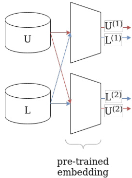
Figure 1. Using pretrained models for constructing views.
图 1: 使用预训练模型构建视图。
Given two pretext tasks we can train a model to accomplish each task, then use their learned embedding spaces as separate views for classification. If we have chosen our pretext tasks well, then the representations will be different, compressed, and capture sufficient information to perform the desired downstream task. Figure 1 demonstrates the idea of the method. Even if one does not have access to different views on a particular dataset, the use of different pre-trained models allows the creation of different views; as the transformation happens at the level of instances, it applies to both labeled and unlabeled batches alike as shown in Figure 1 with $L$ and $U$ respectively. However, if one has access to a dataset where the instances have two different views, then one can still obtain useful representations with this approach using even the same pre-trained model. Furthermore, one can also use multiple pre-trained models and concatenate the resulting embeddings so that two separate views with richer information content can be created and are still low-dimensional.
给定两个前置任务,我们可以训练一个模型来完成每个任务,然后将其学习到的嵌入空间作为分类的独立视图。如果我们选择了合适的前置任务,这些表征将具有差异性、经过压缩且能捕获足够信息以执行目标下游任务。图 1: 展示了该方法的核心思想。即使无法获取特定数据集的多重视角,使用不同预训练模型也能创建差异化视图;由于转换发生在实例层面,该方法可同时适用于带标签 ($L$) 和无标签 ($U$) 批次数据,如图 1: 所示。若数据集本身包含实例的双重视角,即使使用相同预训练模型也能通过此方法获得有效表征。此外,还可组合多个预训练模型并拼接生成嵌入,从而创建信息更丰富且仍保持低维度的双重视图。
While our approach is more widely applicable, it is particularly well-suited to computer vision. There are a plethora [19, 20, 23, 24, 38, 42, 49, 58, 61] of competitive learned representations for images. Recently it has been popular to treat these representations as task-agnostic foundation models. We show that the existence of these models eliminates the need to train new models for pretext tasks to achieve state-of-the-art performance for SSL-classification. Furthermore, it is comparatively very cheap to use the foundation models instead as not only can we forego training on a pretext task, but we are able to completely bypass the need to train a large convolutional neural network (CNN) or vision transformer (ViT). In fact, we compute the embedding for each of the images in our dataset only one time (as opposed to applying some form of data augmentation during training and making use of the embedding process during training). So, at training time the only weights we need to use at all are those in the model we train on top of the learned representation. This makes our approach incredibly lightweight compared to traditional CNN/ViT training procedures.
虽然我们的方法具有更广泛的适用性,但它尤其适合计算机视觉领域。目前存在大量 [19, 20, 23, 24, 38, 42, 49, 58, 61] 针对图像的优秀学习表征方法。近年来,将这些表征视为任务无关的基础模型 (foundation model) 已成为趋势。我们证明,这些模型的存在消除了为预文本任务训练新模型的需求,同时仍能实现SSL分类的最先进性能。此外,使用基础模型的成本极低——我们不仅能省去预文本任务的训练过程,还能完全避免训练大型卷积神经网络 (CNN) 或视觉Transformer (ViT) 的需求。实际上,我们仅需对数据集中的每张图像计算一次嵌入表征(而不是在训练期间应用数据增强并重复使用嵌入过程)。因此训练阶段唯一需要更新的权重,就是基于学习表征所训练模型的参数。这使得我们的方法相比传统CNN/ViT训练流程极为轻量化。
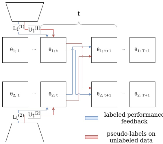
Figure 2. At each step $t~\in~{1,\ldots,T}$ of meta co-training the models that correspond to the so-far learnt parameters $\theta_{1;t}$ and $\theta_{2;t}$ play the role of the student and the teacher simultaneously using batches for their respective views. Pseudo-labeling occurs on complementary views so that the teacher can provide the student with labels on an unlabeled batch. Labeled batches may, or may not, use complementary views as the purpose that they serve is to calculate the risk of the student model on the labeled batch and this result signals the teacher model to update its weights accordingly.
图 2: 在元协同训练的每个步骤 $t~\in~{1,\ldots,T}$ 中,对应于当前学习参数 $\theta_{1;t}$ 和 $\theta_{2;t}$ 的模型同时扮演学生和教师的角色,分别使用各自视角的批次数据。伪标注发生在互补视角上,使得教师能够为未标注批次提供标签。标注批次可能使用也可能不使用互补视角,其目的是计算学生模型在标注批次上的风险,该结果会提示教师模型相应地更新其权重。
4.2. Meta Co-Training
4.2. Meta 协同训练
In addition to our method of view construction we propose a novel algorithm for co-training which is based on Meta Pseudo Labels [59], called Meta $_{C o}$ -Training (MCT), which is described below.
除了我们的视图构建方法外,我们还提出了一种基于元伪标签[59]的新型协同训练算法,称为Meta $_{Co}$-Training (MCT),具体描述如下。
4.2.1 Overview of Meta Co-Training (MCT)
4.2.1 Meta Co-Training (MCT) 概述
An overview of MCT is provided in Figure 2. At each step $t~\in~{1,\ldots,T}$ of meta co-training the models that correspond to the so-far learnt parameters $\theta_{1;t}$ and $\theta_{2;t}$ play the role of the student and the teacher simultaneously on batches from their respective views. The (low-dimensional) embeddings obtained from the view construction process of Section 4.1 form different views that are used by MCT.
图 2 展示了 MCT (Meta Co-Training) 的概览。在元协同训练的每个步骤 $t~\in~{1,\ldots,T}$ 中,对应已学习参数 $\theta_{1;t}$ 和 $\theta_{2;t}$ 的模型会同时在各自视图的批次数据上扮演学生和教师的双重角色。通过 4.1 节视图构建过程获得的 (低维) 嵌入形成了 MCT 所使用的不同视图。
When a student model predicts labels on an unlabeled batch it suffers loss based on the pseudo-labels that are provided by the teacher model (which uses the complementary view for the unlabeled instances) and the student weights are adjusted accordingly. Then the student model evaluates the performance of its new weights on separate labeled batches. This performance provides feedback to the teacher model. Geometrically, we can understand this as updating the parameters in the direction of increasing confidence on our pseudo labels if those labels helped the other model perform better on the labeled set, or in the opposite direction if it hurt the other model’s performance on the labeled set.
当学生模型在未标记批次上预测标签时,它会基于教师模型提供的伪标签(该模型使用未标记实例的互补视角)产生损失,并相应调整学生模型的权重。随后,学生模型在独立的已标记批次上评估其新权重的性能。该性能会向教师模型提供反馈。从几何角度理解,若这些伪标签能帮助另一模型在已标记集上表现更好,则参数更新方向会朝着提升伪标签置信度的方向进行;反之,若损害另一模型在已标记集上的性能,则朝相反方向更新参数。
Finally, similar to MPL, we assume that at $t=1$ models
最后,与MPL类似,我们假设在 $t=1$ 时模型
have been pre-trained using supervised warmup period so that their predictions are not random. This is analogous to the fully-supervised iteration of co-training.
已通过监督预热期进行预训练,使其预测结果不再随机。这类似于协同训练的全监督迭代过程。
4.2.2 Algorithmic Details
4.2.2 算法细节
Algorithm 1 presents the details in pseudocode. The function Sample Batch, is sampling a batch from the dataset. The function get Other View returns the complementary view of the first argument; the second argument clarifies which view should be returned (“2” in line 5). At each step $t$ of the algorithm each model is first updated based on the pseudo labels the other has provided on a batch of unlabeled data (Lines 13-14). Then each model is updated to provide labels that encourage the other to predict more correctly on the labeled set based on the performance of the other (Lines 24-25). We refer the reader to Section 3.2 (resp. [59]) for a brief (resp. complete) discussion of the MPL approach. Note that contrary to traditional co-training, no new pseudo-labeled data are added to the labeled set, neither are any data removed from the unlabeled set after each step.
算法1以伪代码形式展示了具体细节。函数Sample Batch从数据集中采样一个批次。函数getOtherView返回第一个参数的互补视图;第二个参数说明应返回哪个视图(第5行的"2")。在算法的每个步骤$t$中,首先基于另一个模型在未标记数据批次上提供的伪标签更新每个模型(第13-14行)。然后根据对方在标记集上的表现,更新每个模型以提供能促使对方预测更准确的标签(第24-25行)。关于MPL方法的简要(完整)讨论,请参阅3.2节(以及[59])。请注意与传统协同训练不同,每个步骤后既不会向标记集添加新的伪标记数据,也不会从未标记集中移除任何数据。
Table 1. Linear probe evaluation for views. Top-1 accuracy on different subsets of the ImageNet data are shown.
表 1: 视图线性探针评估结果。展示ImageNet数据不同子集的Top-1准确率。
| 模型 | 1% | 10% | 100% |
|---|---|---|---|
| MAE | 1.9 | 3.2 | 73.5 |
| DINOv2 | 78.1 | 82.9 | 86.3 |
| SwAV | 12.1 | 41.1 | 77.9 |
| EsViT | 69.1 | 74.4 | 81.3 |
| CLIP | 74.1 | 80.9 | 85.4 |
5. Experimental Evaluation
5. 实验评估
Towards evaluating the proposed method of view construction for co-training we first constructed views of the data utilizing five different learned representations. Our primary comparisons were on the widely-used ImageNet [31] classification task; however, Sections 5.4 and B provide experimental results on additional image classification tasks. To produce the views used to train the class if i ers during cotraining and meta co-training we used the embedding space of five representation learning architectures: The Masked Autoencoder (MAE) [42], DINOv2 [58], SwAV [19], EsViT [49], and CLIP [61]. We selected the models which produce the views as they have been learned in an unsupervised way, have been made available by the authors of their respective papers for use in PyTorch, and have been shown to produce representations that are appropriate for ImageNet classification.
为评估所提出的协同训练视图构建方法,我们首先利用五种不同的学习表征构建数据视图。主要对比实验基于广泛使用的ImageNet[31]分类任务,第5.4节和附录B还提供了其他图像分类任务的实验结果。在协同训练和元协同训练过程中,我们使用五种表征学习架构的嵌入空间来生成分类器训练视图:掩码自编码器(MAE)[42]、DINOv2[58]、SwAV[19]、EsViT[49]和CLIP[61]。选择这些模型生成视图的原因是:它们采用无监督方式训练、原作者提供了PyTorch实现、且已证明能生成适用于ImageNet分类的表征。
5.1. Investigating the Co-Training Assumptions on the Constructed Views
5.1. 基于构建视图的协同训练假设研究
Table 2. MLP performance on individual views. Top-1 accuracy on different subsets of the ImageNet data are shown.
表 2: 各视角下 MLP 的性能表现。展示了 ImageNet 数据不同子集的 Top-1 准确率。
| Model | 1% | 10% |
|---|---|---|
| MAE | 23.4 | 48.5 |
| DINOv2 | 78.4 | 82.7 |
| SwAV | 12.5 | 32.6 |
| EsViT | 71.3 | 75.8 |
| CLIP | 75.2 | 80.9 |
Motivated by the analysis and experiments of [34] we made an effort to verify the sufficiency and independence of the representations learned by the aforementioned models.
受[34]的分析和实验启发,我们致力于验证上述模型所学表征的充分性与独立性。
On the Sufficiency of the Views. Sufficiency is fairly easy to verify. If we choose a reasonable sufficiency threshold for the task, for ImageNet say close or above $70%$ top-1 accuracy, then we can train simple models on the views of the dataset we have constructed and provide examples of functions which demonstrate the satisfaction of the property. We tested a single linear layer with softmax output, as well as a simple 3-layer multi-layer perceptron (MLP) with 1024 neurons per layer and dense skip connections (previous layer outputs were concatenated to input for subsequent layers) to provide a lower bound on the sufficiency of the views on the standard subsets of the ImageNet labels for semi-supervised classification. From these experiments, whose results are shown in Tables 1 and 2 re sep ect iv ely, we can see that if we were to pick a threshold for top-1 accuracy around $70%$ , which we believe indicates considerable skill without presenting too high of a bar, then EsViT, CLIP, and DINOv2 provide sufficient views for both the $1%$ and
关于视图的充分性。充分性相当容易验证。如果我们为任务选择一个合理的充分性阈值,例如ImageNet接近或高于70%的top-1准确率,那么我们可以在构建的数据集视图上训练简单模型,并提供满足该属性的函数示例。我们测试了带softmax输出的单线性层,以及每层1024个神经元并带有密集跳跃连接(前一层的输出与后续层的输入拼接)的简单3层多层感知机(MLP),以提供ImageNet标准子集在半监督分类任务中视图充分性的下限。从这些实验结果(分别如表1和表2所示)可以看出,若将top-1准确率阈值设定在70%左右(我们认为这表明了相当的能力且门槛不过高),那么EsViT、CLIP和DINOv2在1%和...
Table 3. Pairwise translation performance of linear probe on the ImageNet dataset. A linear classifier is trained on the output of an MLP which is trained to predict one view (columns) from another view (rows) by minimizing MSE. The top-1 accuracy $(%)$ of the linear classifier is reported. Both the MLP and the linear classifier have access to the entire embedded ImageNet training set.
表 3: ImageNet数据集上线性探针的成对翻译性能。通过最小化均方误差 (MSE) 训练一个多层感知机 (MLP) 从一种视图 (行) 预测另一种视图 (列),并在其输出上训练线性分类器。报告线性分类器的 top-1 准确率 $(%)$。MLP 和线性分类器均可访问整个嵌入的 ImageNet 训练集。
| MAE | DINOv2 | SwAV | EsViT | CLIP | |
|---|---|---|---|---|---|
| MAE | 0.139 | 0.142 | 0.137 | 0.129 | |
| DINOv2 | 0.110 | 0.132 | 0.135 | 0.130 | |
| SwAV | 0.116 | 0.147 | 0.137 | 0.126 | |
| EsViT | 0.112 | 0.140 | 0.116 | 0.135 | |
| CLIP | 0.110 | 0.146 | 0.136 | 0.156 |
$10%$ subsets.
10% 子集
On the Independence of the Views. To test the independence of the views generated by the representation learning models, we trained an identical MLP architecture to predict each view from each other view; Table 3 presents our findings, explained below. Given as input the view to predict from (rows of Table 3) the MLPs were trained to reduce the mean squared error (MSE) between their output and the view to be predicted (columns of Table 3). We then trained a linear classifier on the outputs generated by the MLP given every training set embedding from each view. Had the model faithfully reconstructed the output view given only the input view then we would expect the linear classifier to perform similarly to the last column of Table 1. The linear class if i ers never did much better than a random guess on the ImageNet class achieving at most $0.156%$ accuracy. Thus, while we cannot immediately conclude that the views are independent, it is clearly not trivial to predict one view given any other. We believe that this is compelling evidence for the independence of different representations.
视图独立性验证
为测试表征学习模型生成视图的独立性,我们训练了相同的多层感知机(MLP)架构,通过任一视图预测其他视图。表3展示了实验结果,具体分析如下:
给定输入视图(表3的行),MLP通过最小化输出与待预测视图(表3的列)之间的均方误差(MSE)进行训练。随后,我们在MLP基于各视图训练集嵌入生成的输出上训练线性分类器。若模型能仅凭输入视图准确重构输出视图,线性分类器的性能应接近表1最后一列的结果。
实际测试中,线性分类器在ImageNet类别上的最高准确率仅为$0.156%$,与随机猜测无异。虽然不能直接断言视图完全独立,但实验表明:基于任一视图预测其他视图具有显著难度。我们认为这为不同表征的独立性提供了有力证据。
(注:根据规则要求,已对表格引用格式、专业术语、数学符号等进行标准化处理,并确保技术表述的准确性。)
5.2. Experimental Evaluation on ImageNet
5.2. ImageNet 上的实验评估
Having constructed at least two strong views of the data, and suspecting that these views are independent we hypothesize that co-training will work on this data. In Table 4a we show the results of applying the standard co-training algorithm [12]. At each iteration of co-training the model made
在构建了至少两个数据强视图并怀疑这些视图独立后,我们假设协同训练(co-training)将适用于此数据。表4a展示了应用标准协同训练算法[12]的结果。在协同训练的每次迭代中,模型会...
(a) Co-Training
| DINOv2 | SwAV | EsViT | CLIP | |
|---|---|---|---|---|
| MAE | 81.8 (75.5) | 30.5 (11.4) | 77.1 (66.2) | 78.8 (66.8) |
| DINOv2 | 78.5 (74.5) | 83.3 (78.9) | 85.1 (80.1) | |
| SwAV | 70.6 (64.9) | 75.5 (67.4) | ||
| EsViT | 82.3 (76.9) |
(a) 协同训练
(b) Meta Co-Training
| DINOv2 | SwAV | EsViT | CLIP | |
|---|---|---|---|---|
| MAE | 81.2 (73.8) | 37.6 (8.1) | 73.6 (63.8) | 78.6 (63.5) |
| DINOv2 | 77.3 (70.7) | 83.4 (79.2) | 85.2 (80.7) | |
| SwAV | 74.4 (67.3) | 77.1 (67.4) | ||
| EsViT | 82.4 (77.5) |
(b) 元协同训练 (Meta Co-Training)
Table 4. Co-training and meta co-training top-1 accuracy of view combinations on $10%$ $(1%)$ of ImageNet labels. As co-training does not depend on the order of the views, we show only upper-diagonal entries of the pairwise comparison. Diagonal entries would correspond to views which are trivially dependent. All ${\binom{5}{2}}=10$ different combinations of views are shown in each table.
表 4: 在 ImageNet 标签的 $10%$ $(1%)$ 数据上,不同视图组合的协同训练 (co-training) 和元协同训练 (meta co-training) 的 top-1 准确率。由于协同训练不依赖于视图的顺序,我们仅展示成对比较的上三角部分。对角线部分对应的是具有平凡依赖关系的视图。每个表格展示了 ${\binom{5}{2}}=10$ 种不同的视图组合。
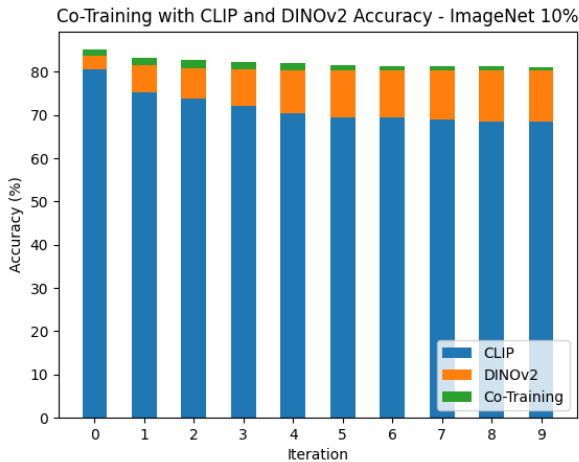
Figure 3. Top-1 accuracy of co-training iterations on the CLIP and DINOv2 views for the ImageNet $10%$ dataset.
图 3: ImageNet $10%$ 数据集上 CLIP 和 DINOv2 视图协同训练迭代的 Top-1 准确率。
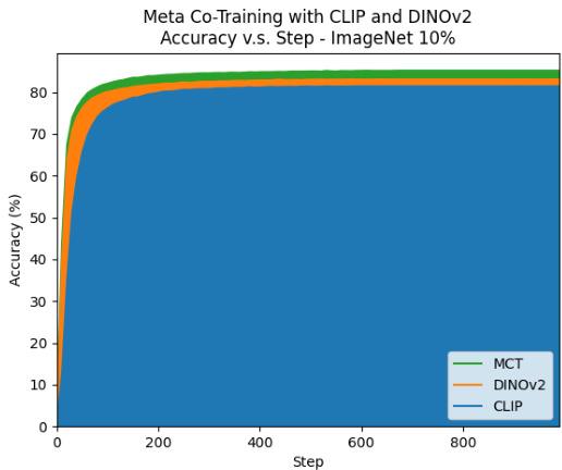
Figure 4. Meta co-training using the CLIP and DINOv2 views as a function of the training step. Models are trained on $10%$ of the ImageNet labels.
图 4: 使用CLIP和DINOv2视图进行元协同训练的效果随训练步数的变化。模型在ImageNet数据集中10%的标注数据上进行训练。
a prediction for all of the instances in $U$ , following (4). We assigned labels to the $10%$ of the total original unlabeled data with most confident predictions for both models. When confident predictions conflicted on examples, we returned those instances to the unlabeled set, otherwise they entered the labeled set of the other model with the assigned pseudolabel.
按照(4)式对$U$中的所有实例进行预测。我们将总原始未标记数据中预测置信度最高的$10%$分别分配给两个模型。当示例的置信预测发生冲突时,我们将这些实例返回到未标记集,否则它们会以分配的伪标签进入另一个模型的标记集。
Predicting according to (4) yielded better accuracy than the predictions of each individual model. In addition, in our experiments on ImageNet, as co-training iterations proceeded top-1 accuracy decreased. Later we show that this was not always the case (see Figure 11 in the appendix). The decrease was less pronounced when the views perform at a similar level; see Figure 3. However, meta co-training does not exhibit performance degradation - in fact this is an ideal case where the method performs best; see Figure 4. While Figures 3 and 4 correspond to ImageNet $10%$ , similar observations also hold for ImageNet $1%$ ; please see the appendix.
根据(4)进行预测比单个模型的预测准确率更高。此外,在ImageNet实验中,随着协同训练迭代进行,top-1准确率出现下降(附录图11显示并非总是如此)。当视图性能相近时,下降幅度较小(见图3)。但元协同训练不会出现性能衰减——这实际上是该方法表现最佳的理想情况(见图4)。虽然图3和图4对应ImageNet $10%$ 数据,但类似现象也出现在ImageNet $1%$ 数据中(详见附录)。
Comparing co-training accuracy on ImageNet $10%$ (resp. $1%$ ) shown in Table 4a compared to MLP accuracy shown in Table 2, we observe that co-training top-1 accuracy is on average $18.7%$ (resp. $16.8%,$ ) higher than MLP accuracy. Moreover, the best co-training top-1 accuracy is $2.4%$ (resp. $1.7%$ ) higher compared to the best top-1 MLP accuracy. In other words, co-training resulted in a significant increase in prediction accuracy but not after the warmup iteration finished. Meta co-training, however, continues to improve after the warmup period has elapsed. See Figures 5 and 6 for a comparison in the case of ImageNet $10%$ ; a similar comparison for ImageNet $1%$ is presented in the appendix.
比较ImageNet上协同训练的准确率
如表4a所示,在ImageNet $10%$ (或 $1%$) 数据上,协同训练的top-1准确率平均比表2中MLP的准确率高 $18.7%$ (或 $16.8%$)。此外,最佳协同训练top-1准确率比最佳MLP top-1准确率高 $2.4%$ (或 $1.7%$)。换言之,协同训练显著提高了预测准确率,但这一提升并非发生在预热迭代完成后。而元协同训练在预热期结束后仍持续改进。关于ImageNet $10%$ 数据的对比,请参见图5和图6;ImageNet $1%$ 数据的类似对比见附录。
Despite the poor performance of the pseudo-labeling during co-training, using the two best performing views in (4) performed as well as the previous SotA method for semi-supervised classification on the ImageNet $10%$ ; see Co-Training in Table 5. The performance of co-training as a method was rather disappointing in that the algorithm is unable to leverage pseudo-labels to improve the accuracy on this task; however, the results do show that our view-construction method has merit. Given the difficulty of translating between the views, and the fact that the accuracy yielded by (4) is greater than its constituent views, we believe the poor performance of the pseudo-labeling step in co-training was due to low information content of at least one view rather than view-dependence.
尽管协同训练中伪标签的表现不佳,但使用(4)中两个性能最佳的视图进行半监督分类时,其表现与之前在ImageNet $10%$ 上的SotA方法相当;参见表5中的协同训练部分。作为一种方法,协同训练的表现相当令人失望,因为该算法无法利用伪标签来提高此任务的准确性;然而,结果确实表明我们的视图构建方法具有价值。考虑到视图间转换的困难,以及(4)产生的准确性高于其组成视图的事实,我们认为协同训练中伪标签步骤表现不佳的原因是至少一个视图的信息量较低,而非视图依赖性。
| 参考文献 | 模型 | 方法 | ImageNet-1% | ImageNet-10% |
|---|---|---|---|---|
| [49] | EsViT (Swin-B, W=14) | Linear | 69.1 | 74.4 |
| [42] | MAE (ViT-L) | MLP | 23.4 | 48.5 |
| [61] | CLIP (ViT-L) | Fine-tuned | 80.5 | 84.7 |
| [58] | DINOv2 (ViT-L) | Linear | 78.1 | 82.9 |
| [24] | SimCLRv2 (ResNet152-w2) | Fine-tuned | 74.2 | 79.4 |
| [61] | SwAV (RN50-w4) | Fine-tuned | 53.9 | 70.2 |
| [60] | Deep Co-Training (ResNet-18) | Co-Training | 53.5 | |
| [17] | Semi-ViT (ViT-L) | Self-trained | 77.3 | 83.3 |
| [52] | REACT (ViT-L) | REACT | 81.6 | 85.1 |
| [59] | MPL (EfficientNet-B6-Wide) | MPL | 73.9 | |
| [12] | Co-Training (MLP)* | Co-Training | 80.1 | 85.1 |
| MCT (MLP)* -ours | MCT | 80.7 | 85.8 |
Table 5. Performance of different approaches on ImageNet dataset. An asterisk $({}^{*})$ indicates models that were trained on top of embeddings generated by much larger models. During training we do not need to alter the parameters of these larger models, and these larger models need not see data used for downstream classification during their training, however training of downstream models would not have been possible without the embeddings. Models on the lower half of the table use unlabeled data during classification training.
表 5: ImageNet数据集上不同方法的性能。带星号 $({}^{*})$ 的模型是在由更大模型生成的嵌入(embedding)基础上训练的。在训练过程中,我们无需修改这些大模型的参数,且这些大模型在其训练期间无需接触下游分类任务的数据,但若没有这些嵌入,下游模型的训练将无法进行。表格下半部分的模型在分类训练时使用了未标注数据。

Figure 5. Top-1 accuracy of co-training iterations for the ImageNet $10%$ dataset. The average over all 10 pairs, the best pair, and the worst pair at each iteration are shown.
图 5: ImageNet 10% 数据集上协同训练迭代的 Top-1 准确率。展示了所有 10 对组合的平均值、最佳组合和最差组合在每次迭代中的表现。
5.2.1 More on Meta Co-Training
5.2.1 关于元协同训练的更多内容
To draw fair comparisons we fix the model architecture and view set from our experiments on co-training. As in MPL [59] a supervised loss is optimized jointly with a loss on pseudo-labels. Like MPL, we found that beginning with a warmup period in which the model trained in a strictly supervised way expedited training. This warmup period occurs for the same number of updates as the first training phase of co-training, so each method starts with the same number of supervised updates before pseudo-labeling. Unlike MPL, we did not use Unsupervised Data Augmentation [75], because we embedded the dataset only once, and due to the nature of the pretext tasks that were used to generate the views we did not believe data augmentation would have much of an effect. Details of our training recipe appear in Table 10.
为了进行公平比较,我们固定了协同训练实验中的模型架构和视图集。与MPL[59]类似,我们同时优化监督损失和伪标签损失。与MPL相同,我们发现以严格监督方式启动模型训练的预热期能加速训练过程。该预热期的更新次数与协同训练第一阶段相同,因此各方法在开始伪标注前都经过相同次数的监督更新。不同于MPL的是,我们没有使用无监督数据增强[75],因为数据集仅被嵌入一次,且基于生成视图的预训练任务特性,我们认为数据增强效果有限。具体训练方案详见表10。

Figure 6. Aggregate statistics of meta co-training across all views. Models are trained on $10%$ of the ImageNet labels. The maximum performance of any pair, the minimum performance of any pair, and the average of all 10 pairs is shown.
图 6: 跨所有视图的元协同训练汇总统计。模型在ImageNet标签的$10%$上训练。展示了任意配对的最大性能、任意配对的最小性能以及所有10个配对的平均性能。
Comparing the top-1 accuracy of MCT and co-training on ImageNet $10%$ (resp. $1%$ ) shown in Table 5, we observe that MCTyielded a difference on average $0.7%$ (resp. $-0.6%)$ ) compared to co-training. Moreover, MCT top-1 accuracy is $0.1%$ (resp. $0.6%$ ) higher overall. Note that on all view pairs in which co-training beats MCT, apart from the $10%$ (EsViT, MAE) pair, one of the views alone was better than co-training. The single DINOv2 view outperforms all such view pairs. These are all cases in which one of the views was significantly weaker than the other. For the experiments in which we had two strong (e.g., not SwAV or MAE)
比较MCT和协同训练在ImageNet上10%(或1%)数据的top-1准确率(如 表5 所示),我们观察到MCT相比协同训练平均有0.7%(或-0.6%)的差异。此外,MCT的top-1准确率总体高出0.1%(或0.6%)。值得注意的是,在所有协同训练优于MCT的视图组合中,除了10%(EsViT、MAE)这一组外,单独使用其中一个视图的效果都比协同训练更好。而单一的DINOv2视图在所有这类视图组合中都表现更优。这些情况都出现在其中一个视图明显弱于另一个视图时。在我们使用两个强视图(即非SwAV或MAE)的实验中...
Table 6. Co-training and MCT evaluated on the ImageNet dataset using the CLIP EsViT and DINOv2 SwAV views.
表 6: 在ImageNet数据集上使用CLIP EsViT和DINOv2 SwAV视图评估协同训练(Co-training)和MCT
| 方法 | 1% | 10% |
|---|---|---|
| 协同训练(Co-Training) | 80.0 | 84.8 |
| MCT | 80.5 | 85.8 |
Table 7. Additional Comparisons to REACT [52]. The authors include experiments for zero-shot performance and $10%$ of available labels. Results above are for $10%$ of labels. For Flowers102 this is 1-shot performance.
表 7: 与REACT [52]的额外对比。作者包含了零样本性能和使用10%可用标签的实验结果。上述结果为使用10%标签时的表现。对于Flowers102数据集,这是单样本性能。
| 方法 | Flowers102 | Food101 | FGVCAircraft |
|---|---|---|---|
| REACT (ViT-L) | 97.0 | 85.6 | 57.1 |
| Co-Training (MLP) | 99.2 | 94.7 | 36.4 |
| MCT (MLP) | 99.6 | 94.8 | 40.1 |
Table 8. Additional Comparisons to Semi-ViT using $10%$ $(1%)$ of the available labels for training. For the i Naturalist task we use only the 1010 most frequent classes as in [17].
表 8: 使用 $10%$ $(1%)$ 可用标签进行训练时与 Semi-ViT 的额外对比。对于 iNaturalist 任务,我们仅使用 [17] 中所述的 1010 个最频繁类别。
| 方法 | 数据集 | |
|---|---|---|
| iNaturalist | Food101 | |
| Semi-ViT (ViT-B) | 67.7 (32.3) | 84.5 (60.9) |
| Co-Training (MLP) | 59.7 (29.5) | 94.7 (83.9) |
| MCT (MLP) | 76.0 (58.1) | 94.8 (91.7) |
views, MCT always performed better than co-training.
观点方面,MCT的表现始终优于协同训练。
5.3. Stronger Views by Concatenation
5.3 通过串联强化观点
Finally, we take the four views which had the greatest performance and constructed two views out of them by concatenating them together. We constructed one view CLIP EsViT and the second DINOv2 SwAV and measured the performance of co-training and meta co-training on these views in Table 6. Interestingly, co-training does not benefit from these larger views; see Table 6.
最后,我们选取了性能最佳的四种视图,通过将它们拼接在一起来构建两种视图。我们构建了第一个视图 CLIP EsViT 和第二个视图 DINOv2 SwAV,并在表 6 中测量了在这些视图上进行协同训练和元协同训练的性能。有趣的是,协同训练并未从这些更大的视图中受益;参见表 6。
The additional information may have allowed the individual models to overfit their training data quickly. During meta co-training we observed that after one model reaches $100%$ training accuracy, its validation accuracy can still improve by learning to label for the other model. Possibly due to the rapid over fitting due to the increased view size (and consequently increased parameter count) the $1%$ split did not show improvement for either model.
额外的信息可能让各个模型迅速过拟合其训练数据。在元协同训练过程中我们观察到,当一个模型达到 $100%$ 训练准确率后,其验证准确率仍可通过学习为另一模型标注而提升。可能是由于视图尺寸增大(进而参数数量增加)导致的快速过拟合, $1%$ 数据分片未对任一模型表现出提升效果。
5.4. Experiments on Additional Datasets
5.4. 其他数据集的实验
In Tables 7 and 8 we compare MCT and co-training to existing SotA approaches that leverage unlabeled data directly during training (e.g., not just part of a pretext task). These experiments support our hypothesis that the primary cause of the failure of co-training is that one or more views can be weak and do not suffice to learn a model that achieves reasonably high accuracy. The closer to equivalent in performance individual views are, the less the performance suffers. When the two views perform similarly and well, the performance improves. Section B in the appendix provides more information on these additional datasets; Figure 11 provides an example where co-training performs as expected and accuracy increases as co-training progresses. The main takeaway of these additional experiments, apart from establishing new SotA results in datasets beyond ImageNet, is that MCT is in general more robust to view imbalance and provides better results than co-training.
在表7和表8中,我们将MCT和协同训练与直接在训练过程中利用未标注数据的现有SotA方法进行了比较(例如,不仅仅是作为前置任务的一部分)。这些实验支持了我们的假设:协同训练失败的主要原因是其中一个或多个视图可能较弱,不足以学习出达到合理高准确率的模型。各视图性能越接近,性能下降就越小。当两个视图表现相似且良好时,性能会有所提升。附录中的B部分提供了关于这些额外数据集的更多信息;图11展示了一个协同训练按预期进行且准确率随训练进程提升的案例。除了在ImageNet之外的数据集上建立新的SotA结果外,这些额外实验的主要结论是:MCT通常对视图不平衡更具鲁棒性,并能提供比协同训练更好的结果。
6. Conclusion and Future Work
6. 结论与未来工作
We presented a novel method of view construction for cotraining approaches based on pretext tasks. We showed that the constructed views likely contain independent information and that models trained on these views can complement each other to produce stronger class if i ers. These views allowed co-training to match the SotA on ImageNet $10%$ . We proposed meta co-training, a novel co-training algorithm. We showed that our algorithm outperforms co-training in general, and establishes a new SotA top-1 classification accuracy on the ImageNet $10%$ as well as new SotA few-shot top-1 classification accuracy on other popular CV datasets.
我们提出了一种基于前置任务(pretext task)的协同训练视图构建新方法。研究表明,所构建的视图可能包含独立信息,且在这些视图上训练的模型能够相互补充,从而构建更强的分类器。该方法使协同训练在ImageNet $10%$ 数据集上达到了当前最优水平(SotA)。我们提出了元协同训练(meta co-training)这一新型协同训练算法,该算法在整体性能上优于传统协同训练,不仅在ImageNet $10%$ 数据集上创造了新的SotA top-1分类准确率记录,同时在其他主流CV数据集上实现了少样本(few-shot)top-1分类准确率的新SotA。
For future work we expect that fine-tuning the representation learners that we used for co-training and MCT would yield better results; which should be in line to observations from papers proposing foundation models that report performance benefits of fine-tuning those models on downstream tasks. Furthermore, we did not make use of the large available unlabeled datasets for computer vision in this study. We suspect that giving our models access to a large repository of unlabeled data as well as the entirety of the labeled data for any dataset on which we performed experiments would result in a performance boost. Finally, our list of pretext tasks was not exhaustive. It is an interesting question for future work which other tasks and models might yield useful views.
在未来工作中,我们预计对协同训练和MCT使用的表征学习器进行微调会取得更好效果,这与提出基础模型的论文中观察到的结论一致——这些论文报告了在下游任务中微调模型带来的性能提升。此外,本研究未利用计算机视觉领域大量可用的未标注数据集。我们推测,若让模型访问大规模未标注数据仓库以及实验数据集的全部标注数据,将带来性能提升。最后,我们的预训练任务清单并非穷尽式列举。未来工作中探索哪些其他任务和模型可能产生有效视图,将是个有趣的研究方向。
Acknowledgements. This material is based upon work supported by the National Science Foundation under Grant No. ICER-2019758. This work is part of the NSF AI Institute for Research on Trustworthy AI in Weather, Climate, and Coastal Oceanography (AI2ES).
致谢。本材料基于美国国家科学基金会资助的工作(资助号: ICER-2019758)。该研究隶属于NSF人工智能研究所"天气、气候与海岸海洋学可信人工智能研究(AI2ES)"项目。
Some of the computing for this project was performed at the OU Super computing Center for Education & Research (OSCER) at the University of Oklahoma (OU).
本项目部分计算工作由俄克拉荷马大学(OU)教育研究超级计算中心(OSCER)完成。
References
参考文献
A. Omitted Experimental Analysis on ImageNet $1%$
A. ImageNet 1% 数据集的省略实验分析
In this section we provide some of the experimental results on ImageNet $1%$ that we did not include into the main text due to space limitations.
在本节中,我们提供了部分在ImageNet $1%$ 上的实验结果,由于篇幅限制未纳入正文。
In Figures 7 and 8 are shown results comparable to those in Figures 3 and 4 in the main text, but for the ImageNet $1%$ dataset. Similar to the case of ImageNet $10%$ we see that the co-training performance decreases after the supervised warmup. Unlike co-training, meta co-training performance increases after the supervised warmup.
图 7 和图 8 展示了与正文中图 3 和图 4 类似的结果,但针对的是 ImageNet $1%$ 数据集。与 ImageNet $10%$ 的情况类似,我们发现协同训练 (co-training) 性能在有监督预热后下降。与协同训练不同,元协同训练 (meta co-training) 性能在有监督预热后有所提升。

Figure 7. Top-1 accuracy of co-training iterations on the CLIP and DINOv2 views for the ImageNet $1%$ dataset.
图 7: ImageNet $1%$ 数据集上 CLIP 和 DINOv2 视图协同训练迭代的 Top-1 准确率。

Figure 8. Meta co-training using the CLIP and DINOv2 views as a function of the training step. Models are trained on $1%$ of the ImageNet labels.
图 8: 使用 CLIP 和 DINOv2 视图进行元协同训练的效果随训练步数的变化。模型在 ImageNet 标签的 $1%$ 数据上训练。
Figures 9 and 10 are comparable to Figures 5 and 6 in the main text, but for the ImageNet $1%$ dataset. The min, max, and mean performance of any of the ten pairs is shown. Note that these are not three runs, but aggregate statistics over all runs, so the minimum and maximum points on the graph for one step may not correspond to the same pair as another step.
图 9 和图 10 与正文中的图 5 和图 6 类似,但针对的是 ImageNet $1%$ 数据集。图中展示了十组实验中每组的最小值、最大值和平均性能。请注意,这些并非三次运行结果,而是所有运行的汇总统计,因此图中某一步骤的最小值和最大值点可能与其他步骤对应的实验组不同。

Co-Training Accuracy - ImageNet 1%
协同训练准确率 - ImageNet 1%

Figure 9. Top-1 accuracy of co-training iterations for the ImageNet $1%$ dataset. The average over all 10 pairs, the best pair, and the worst pair at each iteration are shown. Figure 10. Aggregate statistics of meta co-training across all views. Models are trained on $1%$ of the ImageNet labels. The maximum performance of any pair, the minimum performance of any pair, and the average of all 10 pairs is shown.
图 9: ImageNet $1%$ 数据集上协同训练迭代的 Top-1 准确率。展示了所有 10 对模型的平均结果、最佳配对和最差配对在每次迭代中的表现。
图 10: 跨所有视图的元协同训练汇总统计。模型使用 ImageNet $1%$ 的标签进行训练。展示了任意配对的最大性能、任意配对的最小性能以及所有 10 对模型的平均性能。
B. Further Experimental Analysis on Datasets Beyond ImageNet
B. ImageNet以外数据集的进一步实验分析
Figures 11, 12, 13, 14, 15, 16, and 17 include the top-1 accuracy of co-training using the best (CLIP and DINO) views found for the ImageNet task. In all cases except Figure 11, co-training reaches its maximum performance in the first (warmup) iteration where training is strictly supervised with no pseudo labels. Note that there is no $1%$ run for Flowers102 because there are only 10 examples for each class in the training set (see the discussion in Section C).
图 11、12、13、14、15、16 和 17 展示了在 ImageNet 任务中使用最佳视图 (CLIP 和 DINO) 进行协同训练时的 top-1 准确率。除图 11 外,所有情况下协同训练都在首次 (预热) 迭代中达到最高性能,此时训练完全基于监督学习而未使用伪标签。注意 Flowers102 没有进行 $1%$ 数据量的实验,因为其训练集中每类仅有 10 个样本 (参见附录 C 的讨论)。

Figure 11. The top-1 accuracy of the co-training predictions for each iteration of co-training. $10%$ of available Food101 labels are used for training. The method exhibits performance improvement over multiple iterations of pseudo-labeling and retraining.
图 11: 协同训练每轮迭代的 top-1 准确率。使用 Food101 数据集中 10% 的标注数据进行训练。该方法通过多轮伪标签生成和模型重训练实现了性能提升。

Figure 12. The top-1 accuracy of the co-training predictions for each iteration of co-training. $1%$ of available Food101 labels are used for training.
图 12: 协同训练每轮迭代的 top-1 准确率。使用 Food101 数据集中 $1%$ 的可用标签进行训练。
B.1. Co-Training and Meta Co-Training on Food101
B.1. Food101 数据集上的协同训练与元协同训练
In Figures 11 and 12 we show the top-1 accuracy of the iterations of co-training on the Food101 classification task. Co-training performs as expected with the pseudo labels allowing the other model to improve in the $10%$ case, but in the $1%$ case it appears that one or more of the views was insufficient and the performance decreases rapidly after the first iteration. Co-training achieves top-1 accuracy of $94.7%$ (resp., $83.9%$ ) when $10%$ (resp., $1%$ ) of the available labels for training are used from the Food101 dataset.
在图 11 和图 12 中,我们展示了 Food101 分类任务上协同训练迭代的 top-1 准确率。协同训练在 $10%$ 标签情况下表现符合预期,伪标签能使另一模型性能提升,但在 $1%$ 标签情况下,一个或多个视图信息不足,首轮迭代后性能迅速下降。当使用 Food101 数据集中 $10%$ (对应 $1%$) 的可用训练标签时,协同训练的 top-1 准确率达到 $94.7%$ (对应 $83.9%$)。
Similarly, meta co-training achieves top-1 accuracy of $94.8%$ (resp., $91.7%$ ) when $10%$ (resp., $1%$ ) of the available training examples of the Food101 dataset are used.
同样地,当使用Food101数据集中10%(对应1%)的可用训练样本时,元协同训练实现了94.8%(对应91.7%)的top-1准确率。

Figure 13. The top-1 accuracy of the co-training predictions for each iteration of co-training. Only the $1010\mathrm{most}$ frequent classes are included. $10%$ of available i Naturalist labels from those classes are used for training.
图 13: 协同训练每轮迭代的预测 top-1 准确率。仅包含出现频率最高的 $1010\mathrm{个}$ 类别,并使用这些类别中 $10%$ 的可用 iNaturalist 标签进行训练。

Figure 14. The top-1 accuracy of the co-training predictions for each iteration of co-training. Only the 1010 most frequent classes are included. $1%$ of available i Naturalist labels from those classes are used for training.
图 14: 协同训练每轮迭代的 top-1 准确率。仅包含 1010 个最高频类别,这些类别中 $1%$ 的可用 iNaturalist 标签用于训练。
These results are compared against each other as well as against REACT and Semi-ViT in Tables 7 and 8 respectively.
这些结果相互之间以及与REACT和Semi-ViT的对比分别展示在表7和表8中。
B.2. Co-Training and Meta Co-Training on iNaturalist
B.2. iNaturalist 数据集上的协同训练与元协同训练
In Figures 13 and 14 we show the top-1 accuracy of the iterations of co-training on the i Naturalist dataset. In both splits we see a steady decline in top-1 accuracy after the first iteration. Co-training achieves top-1 accuracy of $59.7%$ (resp., $29.5%,$ when only $10%$ (resp., $1%$ ) of the training examples of the i Naturalist dataset are used.
在图13和图14中,我们展示了i Naturalist数据集上协同训练迭代的top-1准确率。在两个划分中,我们都观察到首次迭代后top-1准确率持续下降。当仅使用i Naturalist数据集$10%$ (对应$1%$)的训练样本时,协同训练实现的top-1准确率为$59.7%$ (对应$29.5%$)。
Along these lines meta co-training achieves $76.0%$ (resp., $58.1%,$ when only $10%$ (resp., $1%$ ) of the training examples of the i Naturalist dataset are used.
按照这些方法,元协同训练在使用iNaturalist数据集中10%(或1%)的训练样本时,准确率分别达到76.0%(或58.1%)。

Figure 15. The top-1 accuracy of the co-training predictions for each iteration of co-training. $10%$ of available FG VC Aircraft labels are used for training.
图 15: 协同训练每轮迭代的 top-1 准确率。训练使用了 10% 可用的 FG VC Aircraft 标签数据。

Figure 16. The top-1 accuracy of the co-training predictions for each iteration of co-training. $1%$ of available FG VC Aircraft labels are used for training.
图 16: 协同训练每轮迭代的top-1准确率。使用 $1%$ 可用FG VC Aircraft标注数据进行训练。
These results are compared against each other as well as against REACT and Semi-ViT in Tables 7 and 8 respectively.
这些结果分别在表7和表8中与REACT和Semi-ViT进行了相互比较。
B.3. Co-Training and Meta Co-Training on CTFG VC Aircraft
B.3. CTFG VC 飞机上的协同训练与元协同训练
In Figures 15 and 16 we show the top-1 accuracy of the iterations of co-training on the C TFG VC Aircraft dataset. In both cases both views have low accuracy, so it is unsurprising that in subsequent iterations the accuracy decreases rapidly. In particular, co-training achieves top-1 accuracy of $36.4%$ (resp., $21.6%)$ when only $10%$ (resp., $1%$ ) of the training examples of the C TFG VC Aircraft dataset are used.
在图 15 和图 16 中,我们展示了在 C TFG VC Aircraft 数据集上协同训练迭代的 top-1 准确率。在这两种情况下,两个视图的准确率都很低,因此在后续迭代中准确率迅速下降也就不足为奇了。具体而言,当仅使用 C TFG VC Aircraft 数据集中 $10%$ (或 $1%$) 的训练样本时,协同训练实现的 top-1 准确率为 $36.4%$ (或 $21.6%$)。
Along these lines meta co-training achieves $40.1%$ (resp., $21.5%$ when only $10%$ (resp., $1%$ ) of the training examples of the C TFG VC Aircraft dataset are used.
沿着这一思路,元协同训练在使用C TFG VC Aircraft数据集仅10%(或1%)的训练样本时,分别达到了40.1%(或21.5%)的准确率。

Figure 17. The top-1 accuracy of the co-training predictions for each iteration of co-training. $10%$ of available Flowers102 labels are used for training.
图 17: 协同训练每轮迭代的Top-1准确率。训练使用了Flowers102数据集中$10%$的可用标签。
The results corresponding to the $10%$ case of co-training and meta co-training are compared against REACT in Table 7, since the authors of [52] report results on zero-shot and $10%$ cases only. However, for completeness, we have decided to include Figure 16 which corresponds to the experiments that we did using only $1%$ of the labeled training data available for the C TFG VC Aircraft dataset.
表7将协同训练和元协同训练在10%数据量下的结果与REACT进行了对比,因为文献[52]的作者仅报告了零样本和10%数据量情况下的结果。但为了完整起见,我们决定加入图16,该图表对应我们仅使用C TFG VC Aircraft数据集中1%标注训练数据进行的实验。
B.4. Co-Training and Meta Co-Training on Flowers102
B.4. Flowers102数据集上的协同训练与元协同训练
As explained earlier, the Flowers102 dataset has only 10 training examples for each class and hence $10%$ corresponds to 1-shot learning. In this context, in Figure 17 we give the performance of the iterations of co-training on the Flowers102 dataset. Even though the DINO view performs very well in the first iteration, there is a large gap between the performance of the CLIP view and the DINO view which leads to decreased performance in subsequent iterations. Co-training achieves top-1 accuracy of $99.2%$ when only $10%$ of the training examples of the Flowers102 dataset are used for training (i.e., a single labeled image per class).
如前所述,Flowers102数据集每个类别仅有10个训练样本,因此$10%$对应1样本学习。在此背景下,图17展示了Flowers102数据集上协同训练迭代的性能表现。尽管DINO视图在第一次迭代中表现优异,但CLIP视图与DINO视图之间存在显著性能差距,导致后续迭代性能下降。当仅使用Flowers102数据集$10%$的训练样本(即每类单张标注图像)时,协同训练的top-1准确率达到$99.2%$。
In the same context of 1-shot learning, meta co-training achieves top-1 accuracy of $99.6%$ .
在同样的1样本学习情境下,元协同训练达到了99.6%的top-1准确率。
Both of the above results are compared against each other and against REACT in Table 7.
表7中将上述两个结果相互比较,并与REACT进行对比。
C. Further Information on the Datasets and the Splits
C. 数据集及划分的更多信息
Table 9 includes a description of the different sizes of the datasets used for training and testing, as well as the number of cases for each dataset. Note that in the $10%$ experiments on the Flowers102 dataset each class has only 1 label. All datasets are approximately class-balanced with the exception of the i Naturalist dataset. In all cases we maintain the original class distribution when sampling subsets. All subsets are created with seeded randomness of a common seed (13) which ensures a fair comparison between methods.
表 9: 包含用于训练和测试的不同规模数据集描述,以及每个数据集的案例数量。需注意,在Flowers102数据集上进行的$10%$实验中,每个类别仅包含1个标签。除iNaturalist数据集外,所有数据集均近似类别平衡。在所有情况下,我们在采样子集时保持原始类别分布。所有子集均采用共同随机种子(13)生成,以确保方法间的公平比较。
Table 9. Sizes of datasets used. Subsets drawn for training are always drawn in a stratified way to maintain the class distribution of the original data. For ImageNet we use the split published with the SimCLRv2 [24] repository.
表 9: 所用数据集规模。训练抽取的子集始终采用分层抽样方式以保持原始数据的类别分布。对于ImageNet数据集,我们采用SimCLRv2 [24]代码库发布的数据划分方案。
| 数据集 | 训练样本数 | 测试样本数 | 类别数 |
|---|---|---|---|
| FGVCAircraft | 3333 | 3333 | 100 |
| Flowers102 | 1020 | 6149 | 102 |
| Food101 | 75,750 | 25,250 | 101 |
| iNaturalist | 175,489 | 29,083 | 1010 |
| ImageNet | 1,281,167 | 50,000 | 1000 |
Table 10. Hyper par meter configuration for meta co-training and co-training. Other models used (MLP, linear) are trained for the same number of steps as meta co-training, with the same optimization parameters.
表 10: 元协同训练和协同训练的超参数配置。其他使用的模型 (MLP, linear) 训练步数与元协同训练相同,优化参数也保持一致。
| config | MCT | Co-Training |
|---|---|---|
| optimizer | Adam | Adam |
| optimizer momentum | β1,β2 = 0.9,0.999 | β1,β2 = 0.9,0.999 |
| base learning rate | 1e-4 | 1e-4 |
| batch size | 4096 | 4096 |
| learning rate schedule | ReduceOnPlateau | ReduceOnPlateau |
| schedule patience | 10 steps | 10 steps |
| decay factor | 0.5 | 0.5 |
| training steps | 1000 | 200 (per iteration) |
| warmup steps | 200 | n/a |
D. Hyper parameter Configuration
D. 超参数配置
The relevant hyper parameters for training are included in Table 10 for co-training and meta co-training (MCT).
训练相关的超参数包含在表10中,用于协同训练(co-training)和元协同训练(MCT)。