Axial-DeepLab: Stand-Alone Axial-Attention for Panoptic Segmentation
Axial-DeepLab: 独立轴向注意力机制的全景分割
Huiyu Wang $\cdot^{\perp\star}$ , Yukun Zhu $^2$ , Bradley Green2, Hartwig Adam $^2$ , Alan Yuille $\perp$ , and Liang-Chieh Chen $^2$
Huiyu Wang $\cdot^{\perp\star}$ , Yukun Zhu $^2$ , Bradley Green $^2$ , Hartwig Adam $^2$ , Alan Yuille $\perp$ , Liang-Chieh Chen $^2$
1 Johns Hopkins University 2 Google Research
1 约翰霍普金斯大学 2 谷歌研究院
Abstract. Convolution exploits locality for efficiency at a cost of missing long range context. Self-attention has been adopted to augment CNNs with non-local interactions. Recent works prove it possible to stack self-attention layers to obtain a fully attention al network by restricting the attention to a local region. In this paper, we attempt to remove this constraint by factorizing 2D self-attention into two 1D selfattentions. This reduces computation complexity and allows performing attention within a larger or even global region. In companion, we also propose a position-sensitive self-attention design. Combining both yields our position-sensitive axial-attention layer, a novel building block that one could stack to form axial-attention models for image classification and dense prediction. We demonstrate the effectiveness of our model on four large-scale datasets. In particular, our model outperforms all existing stand-alone self-attention models on ImageNet. Our Axial-DeepLab improves $2.8%$ PQ over bottom-up state-of-the-art on COCO test-dev. This previous state-of-the-art is attained by our small variant that is $3.8\times$ parameter-efficient and 27 $\times$ computation-efficient. Axial-DeepLab also achieves state-of-the-art results on Mapillary Vistas and Cityscapes.
摘要。卷积利用局部性提升效率,却以牺牲长距离上下文为代价。自注意力机制被引入以增强CNN的非局部交互能力。近期研究证明,通过将注意力限制在局部区域,可以堆叠自注意力层构建全注意力网络。本文尝试通过将二维自注意力分解为两个一维自注意力来突破这一限制,从而降低计算复杂度,并实现在更大甚至全局范围内执行注意力。同时,我们提出位置敏感的自注意力设计。二者结合形成新型基础模块——位置敏感轴向注意力层,可堆叠构建用于图像分类和密集预测的轴向注意力模型。我们在四个大规模数据集上验证了模型有效性:在ImageNet上超越所有现有独立自注意力模型;Axial-DeepLab在COCO test-dev上以$2.8%$ PQ提升超越自底向上方法的最优结果,该记录由我们的小型变体实现(参数效率提升$3.8\times$,计算效率提升$27\times$);在Mapillary Vistas和Cityscapes数据集上也达到最优性能。
Keywords: bottom-up panoptic segmentation, self-attention
关键词:自底向上全景分割 (bottom-up panoptic segmentation)、自注意力 (self-attention)
1 Introduction
1 引言
Convolution is a core building block in computer vision. Early algorithms employ convolutional filters to blur images, extract edges, or detect features. It has been heavily exploited in modern neural networks [50,49] due to its efficiency and generalization ability, in comparison to fully connected models [2]. The success of convolution mainly comes from two properties: translation e qui variance, and locality. Translation e qui variance, although not exact [97], aligns well with the nature of imaging and thus generalizes the model to different positions or to images of different sizes. Locality, on the other hand, reduces parameter counts and M-Adds. However, it makes modeling long range relations challenging.
卷积是计算机视觉的核心构建模块。早期算法使用卷积滤波器来模糊图像、提取边缘或检测特征。与全连接模型 [2] 相比,由于其高效性和泛化能力,卷积在现代神经网络 [50,49] 中被广泛应用。卷积的成功主要源于两个特性:平移等变性 (translation e qui variance) 和局部性 (locality)。平移等变性虽不精确 [97],但与成像本质高度契合,从而使模型能泛化到不同位置或不同尺寸的图像。另一方面,局部性减少了参数量和乘加运算 (M-Adds),但也给建模长距离关系带来了挑战。
A rich set of literature has discussed approaches to modeling long range interactions in convolutional neural networks (CNNs). Some employ atrous convolutions [34,77,67,13], larger kernel [70], or image pyramids [98,85], either designed by hand or searched by algorithms [103,12,60]. Another line of works adopts attention mechanisms. Attention shows its ability of modeling long range interactions in language modeling [83,88], speech recognition [22,11], and neural captioning [92]. Attention has since been extended to vision, giving significant boosts to image classification [6], object detection [37], semantic segmentation [42], video classification [87], and adversarial defense [89]. These works enrich CNNs with non-local or long-range attention modules.
大量文献探讨了在卷积神经网络(CNN)中建模长程交互的方法。部分研究采用空洞卷积(atrous convolutions) [34,77,67,13]、大尺寸卷积核[70]或图像金字塔[98,85],这些方法或通过人工设计或通过算法搜索获得[103,12,60]。另一类工作采用注意力机制,该机制在语言建模[83,88]、语音识别[22,11]和神经图像描述生成[92]中展现了建模长程交互的能力。注意力机制随后被扩展到视觉领域,显著提升了图像分类[6]、目标检测[37]、语义分割[42]、视频分类[87]和对抗防御[89]的性能。这些工作通过非局部或长程注意力模块增强了CNN的能力。
Recently, stacking attention layers as stand-alone models without any spatial convolution has been proposed [68,38] and shown promising results. However, naive attention is computationally expensive, especially on large inputs. Applying local constraints to attention, proposed by [68,38], reduces the cost and enables building fully attention al models. However, local constraints limit model receptive field, which is crucial to tasks such as segmentation, especially on high-resolution inputs. In this work, we propose to adopt axial-attention [33,42], which not only allows efficient computation, but recovers the large receptive field in stand-alone attention models. The core idea is to factorize 2D attention into two 1D attentions along height- and width-axis sequentially. Its efficiency enables us to attend over large regions and build models to learn long range or even global interactions. Additionally, most previous attention modules do not utilize positional information, which degrades attention’s ability in modeling position-dependent interactions, like shapes or objects at multiple scales. Recent works [68,38,6] introduce positional terms to attention, but in a context-agnostic way. In this paper, we augment the positional terms to be context-dependent, making our attention position-sensitive, with marginal costs.
最近,有研究提出将注意力层堆叠为独立模型而不使用任何空间卷积 [68,38],并展现出良好效果。然而,原始注意力计算成本高昂,尤其在大尺寸输入上。[68,38] 提出的局部注意力约束降低了计算量,使全注意力模型成为可能,但会限制模型感受野,这对分割等高分辨率任务至关重要。本文采用轴向注意力 [33,42],既能高效计算,又能恢复独立注意力模型的大感受野。其核心思想是将二维注意力分解为沿高度轴和宽度轴的两次一维注意力计算。这种高效性使我们能够关注大区域,构建学习长程甚至全局交互的模型。此外,多数现有注意力模块未利用位置信息,削弱了其对形状、多尺度物体等位置相关关系的建模能力。近期工作 [68,38,6] 以上下文无关方式引入位置项,而本文通过边际成本将位置项增强为上下文相关,使注意力具备位置敏感性。
We show the effectiveness of our axial-attention models on ImageNet [73] for classification, and on three datasets (COCO [59], Mapillary Vistas [65], and Cityscapes [23]) for panoptic segmentation [48], instance segmentation, and semantic segmentation. In particular, on ImageNet, we build an Axial-ResNet by replacing the $3\times3-$ convolution in all residual blocks [32] with our positionsensitive axial-attention layer, and we further make it fully attention al [68] by adopting axial-attention layers in the ‘stem’. As a result, our Axial-ResNet attains state-of-the-art results among stand-alone attention models on ImageNet. For segmentation tasks, we convert Axial-ResNet to Axial-DeepLab by replacing the backbones in Panoptic-DeepLab [19]. On COCO [59], our Axial-DeepLab outperforms the current bottom-up state-of-the-art, Panoptic-DeepLab [20], by 2.8% PQ on test-dev set. We also show state-of-the-art segmentation results on Mapillary Vistas [65], and Cityscapes [23].
我们在ImageNet[73]分类任务以及三个数据集(COCO[59]、Mapillary Vistas[65]和Cityscapes[23])的全景分割[48]、实例分割和语义分割任务上验证了轴向注意力模型的有效性。具体而言,在ImageNet上,我们通过将所有残差块[32]中的$3\times3-$卷积替换为位置敏感的轴向注意力层,构建了Axial-ResNet模型,并进一步在"stem"结构中采用轴向注意力层使其实现完全注意力机制[68]。最终,我们的Axial-ResNet在ImageNet上取得了独立注意力模型中的最优结果。对于分割任务,我们通过替换Panoptic-DeepLab[19]的主干网络将Axial-ResNet转换为Axial-DeepLab。在COCO[59]测试开发集上,我们的Axial-DeepLab以2.8% PQ的优势超越了当前最先进的自底向上方法Panoptic-DeepLab[20]。我们还在Mapillary Vistas[65]和Cityscapes[23]数据集上取得了最先进的分割结果。
To summarize, our contributions are four-fold:
总结来说,我们的贡献有四点:
– The proposed method is the first attempt to build stand-alone attention models with large or global receptive field. – We propose position-sensitive attention layer that makes better use of positional information without adding much computational cost.
- 所提出的方法是首次尝试构建具有大或全局感受野的独立注意力模型。
- 我们提出了位置敏感注意力层,该层能更好地利用位置信息而无需增加过多计算成本。
– We show that axial attention works well, not only as a stand-alone model on image classification, but also as a backbone on panoptic segmentation, instance segmentation, and segmantic segmentation.
- 我们证明轴向注意力 (axial attention) 不仅能作为图像分类的独立模型表现优异,还能作为全景分割、实例分割和语义分割的主干网络。
– Our Axial-DeepLab improves significantly over bottom-up state-of-the-art on COCO, achieving comparable performance of two-stage methods. We also surpass previous state-of-the-art methods on Mapillary Vistas and Cityscapes.
- 我们的Axial-DeepLab在COCO数据集上显著超越了自底向上(state-of-the-art)方法,达到了与两阶段方法相当的性能。同时,我们在Mapillary Vistas和Cityscapes数据集上超越了之前的最先进方法。
2 Related Work
2 相关工作
Top-down panoptic segmentation: Most state-of-the-art panoptic segmentation models employ a two-stage approach where object proposals are firstly generated followed by sequential processing of each proposal. We refer to such approaches as top-down or proposal-based methods. Mask R-CNN [31] is commonly deployed in the pipeline for instance segmentation, paired with a light-weight stuff segmentation branch. For example, Panoptic FPN [47] incorporates a semantic segmentation head to Mask R-CNN [31], while Porzi et al. [71] append a light-weight DeepLab-inspired module [14] to the multi-scale features from FPN [58]. Additionally, some extra modules are designed to resolve the overlapping instance predictions by Mask R-CNN. TASCNet [52] and AUNet [55] propose a module to guide the fusion between ‘thing’ and ‘stuff’ predictions, while Liu et al. [64] adopt a Spatial Ranking module. UPSNet [91] develops an efficient parameter-free panoptic head for fusing ‘thing’ and ‘stuff’, which is further explored by Li et al. [53] for end-to-end training of panoptic segmentation models. AdaptIS [80] uses point proposals to generate instance masks.
自上而下的全景分割:大多数先进的全景分割模型采用两阶段方法,首先生成目标候选框,再对每个候选框进行序列化处理。我们将这类方法称为自上而下或基于候选框的方法。Mask R-CNN [31] 通常被部署在实例分割流程中,并搭配一个轻量级的语义分割分支。例如,Panoptic FPN [47] 在 Mask R-CNN [31] 基础上增加了语义分割头,而 Porzi 等人 [71] 则在 FPN [58] 的多尺度特征上附加了一个受 DeepLab 启发的轻量级模块 [14]。此外,一些额外模块被设计用于解决 Mask R-CNN 的重叠实例预测问题。TASCNet [52] 和 AUNet [55] 提出了一个模块来指导"物体"和"背景"预测的融合,而 Liu 等人 [64] 则采用了空间排序模块。UPSNet [91] 开发了一种高效的无参数全景头用于融合"物体"和"背景",Li 等人 [53] 进一步探索了该方法用于端到端的全景分割模型训练。AdaptIS [80] 使用点候选框来生成实例掩码。
Bottom-up panoptic segmentation: In contrast to top-down approaches, bottom-up or proposal-free methods for panoptic segmentation typically start with the semantic segmentation prediction followed by grouping ‘thing’ pixels into clusters to obtain instance segmentation. DeeperLab [93] predicts bounding box four corners and object centers for class-agnostic instance segmentation. SSAP [29] exploits the pixel-pair affinity pyramid [63] enabled by an efficient graph partition method [46]. BBFNet [8] obtains instance segmentation results by Watershed transform [84,4] and Hough-voting [5,51]. Recently, PanopticDeepLab [20], a simple, fast, and strong approach for bottom-up panoptic segmentation, employs a class-agnostic instance segmentation branch involving a simple instance center regression [45,82,66], coupled with DeepLab semantic segmentation outputs [13,15,16]. Panoptic-DeepLab has achieved state-of-theart results on several benchmarks, and our method builds on top of it.
自底向上全景分割:与自顶向下方法不同,自底向上或无候选框的全景分割方法通常从语义分割预测开始,随后将"物体"像素聚类以获得实例分割结果。DeeperLab [93] 通过预测与类别无关的边界框四角点和物体中心来实现实例分割。SSAP [29] 利用高效图分割方法 [46] 构建的像素对亲和力金字塔 [63]。BBFNet [8] 采用分水岭变换 [84,4] 和霍夫投票 [5,51] 获取实例分割结果。近期提出的PanopticDeepLab [20] 作为一种简单、快速且强大的自底向上全景分割方案,结合了DeepLab语义分割输出 [13,15,16] 与基于简单实例中心回归 [45,82,66] 的类别无关实例分割分支。Panoptic-DeepLab在多个基准测试中取得了最先进成果,我们的方法正是基于该框架构建。
Self-attention: Attention, introduced by [3] for the encoder-decoder in a neural sequence-to-sequence model, is developed to capture correspondence of tokens between two sequences. In contrast, self-attention is defined as applying attention to a single context instead of across multiple modalities. Its ability to directly encode long-range interactions and its parallel iz ability, has led to state-of-the-art performance for various tasks [83,40,26,69,75,25,56]. Recently, self-attention has been applied to computer vision, by augmenting CNNs with non-local or long-range modules. Non-local neural networks [87] show that selfattention is an instantiation of non-local means [10] and achieve gains on many vision tasks such as video classification and object detection. Additionally, [18,6] show improvements on image classification by combining features from selfattention and convolution. State-of-the-art results on video action recognition tasks [18] are also achieved in this way. On semantic segmentation, self-attention is developed as a context aggregation module that captures multi-scale context [42,27,102,99]. Efficient attention methods are proposed to reduce its complexity [76,42,56]. Additionally, CNNs augmented with non-local means [10] are shown to be more robust to adversarial attacks [89]. Besides disc rim i native tasks, self-attention is also applied to generative modeling of images [95,9,33]. Recently, [68,38] show that self-attention layers alone could be stacked to form a fully attention al model by restricting the receptive field of self-attention to a local square region. Encouraging results are shown on both image classification and object detection. In this work, we follow this direction of research and propose a stand-alone self-attention model with large or global receptive field, making self-attention models non-local again. Our models are evaluated on bottom-up panoptic segmentation and show significant improvements.
自注意力机制 (Self-attention):注意力机制由[3]首次在神经序列到序列模型的编码器-解码器中提出,用于捕捉两个序列间token的对应关系。与之相对,自注意力被定义为在单一上下文而非跨模态间应用注意力机制。其直接编码长程交互的能力与并行化特性,使其在多项任务中取得领先性能[83,40,26,69,75,25,56]。
近期,自注意力通过与非局部或长程模块结合的方式应用于计算机视觉领域。非局部神经网络[87]表明自注意力是非局部均值[10]的实例化,并在视频分类、目标检测等视觉任务中取得提升。此外,[18,6]通过融合自注意力与卷积特征改进了图像分类性能,视频动作识别任务的最优结果[18]也由此实现。在语义分割领域,自注意力被开发为捕捉多尺度上下文的语境聚合模块[42,27,102,99],同时提出了降低计算复杂度的高效注意力方法[76,42,56]。增强非局部均值的CNN[10]还被证明对对抗攻击更具鲁棒性[89]。
除判别式任务外,自注意力也应用于图像生成建模[95,9,33]。最近,[68,38]证明仅通过将自注意力层限制在局部方形感受野内堆叠,即可构建全注意力模型,并在图像分类与目标检测中展现出积极效果。本研究沿袭这一方向,提出具有大范围或全局感受野的独立自注意力模型,使自注意力机制重新具备非局部特性。我们的模型在自底向上全景分割任务中评估,显示出显著改进。
3 Method
3 方法
We begin by formally introducing our position-sensitive self-attention mechanism. Then, we discuss how it is applied to axial-attention and how we build stand-alone Axial-ResNet and Axial-DeepLab with axial-attention layers.
我们首先正式介绍位置敏感的自注意力机制 (position-sensitive self-attention mechanism) 。接着讨论如何将其应用于轴向注意力 (axial-attention) ,以及如何通过轴向注意力层构建独立的 Axial-ResNet 和 Axial-DeepLab 模型。
3.1 Position-Sensitive Self-Attention
3.1 位置敏感自注意力 (Position-Sensitive Self-Attention)
Self-Attention: Self-attention mechanism is usually applied to vision models as an add-on to augment CNNs outputs [87,95,42]. Given an input feature map $\boldsymbol{x}\in\mathbb{R}^{h\times w\times d_{i n}}$ with height $h$ , width $w$ , and channels $d_{i n}$ , the output at position $o=(i,j)$ , $y_{o}\in\mathbb{R}^{d_{o u t}}$ , is computed by pooling over the projected input as:
自注意力 (Self-Attention): 自注意力机制通常作为视觉模型的附加组件来增强CNN输出 [87,95,42]。给定输入特征图 $\boldsymbol{x}\in\mathbb{R}^{h\times w\times d_{i n}}$ (高度 $h$、宽度 $w$、通道数 $d_{i n}$),位置 $o=(i,j)$ 处的输出 $y_{o}\in\mathbb{R}^{d_{o u t}}$ 通过投影输入的池化计算得到:
$$
y_{o}=\sum_{p\in{\cal{N}}}\operatorname{softmax}_ {p}(q_{o}^{T}k_{p})v_{p}
$$
$$
y_{o}=\sum_{p\in{\cal{N}}}\operatorname{softmax}_ {p}(q_{o}^{T}k_{p})v_{p}
$$
where $\mathcal{N}$ is the whole location lattice, and queries $q_{o}=W_{Q}x_{o}$ , keys $k_{o}=W_{K}x_{o}$ , values $v_{o}=W_{V}x_{o}$ are all linear projections of the input $x_{o}\forall o\in\mathcal{N}$ . $W_{Q},W_{K}\in$ $\mathbb{R}^{d_{q}\times d_{i n}}$ and $W_{V}\in\mathbb{R}^{d_{o u t}\times d_{i n}}$ are all learnable matrices. The softmax denotes a $p$ softmax function applied to all possible $\boldsymbol{p}=\left(\boldsymbol{a},\boldsymbol{b}\right)$ positions, which in this case is also the whole 2D lattice.
其中 $\mathcal{N}$ 是整个位置格点,查询 $q_{o}=W_{Q}x_{o}$、键 $k_{o}=W_{K}x_{o}$ 和值 $v_{o}=W_{V}x_{o}$ 都是输入 $x_{o}\forall o\in\mathcal{N}$ 的线性投影。$W_{Q},W_{K}\in$ $\mathbb{R}^{d_{q}\times d_{i n}}$ 和 $W_{V}\in\mathbb{R}^{d_{o u t}\times d_{i n}}$ 都是可学习矩阵。softmax 表示对所有可能的 $\boldsymbol{p}=\left(\boldsymbol{a},\boldsymbol{b}\right)$ 位置(此处也是整个二维格点)应用的 $p$ softmax 函数。
This mechanism pools values $v_{p}$ globally based on affinities $x_{o}^{T}W_{Q}^{T}W_{K}x_{p}$ , allowing us to capture related but non-local context in the whole feature map, as opposed to convolution which only captures local relations.
该机制基于亲和度 $x_{o}^{T}W_{Q}^{T}W_{K}x_{p}$ 全局池化值 $v_{p}$ ,使我们能够捕获整个特征图中相关但非局部的上下文,这与仅捕获局部关系的卷积形成对比。
However, self-attention is extremely expensive to compute $(\mathcal{O}(h^{2}w^{2}))$ when the spatial dimension of the input is large, restricting its use to only high levels of a CNN (i.e., down sampled feature maps) or small images. Another drawback is that the global pooling does not exploit positional information, which is critical to capture spatial structures or shapes in vision tasks.
然而,当输入的空间维度较大时,自注意力 (self-attention) 的计算成本极高 $(\mathcal{O}(h^{2}w^{2}))$ ,这限制了其仅能用于CNN的高层级(即下采样特征图)或小尺寸图像。另一个缺点是全局池化未能利用位置信息,而这对视觉任务中捕捉空间结构或形状至关重要。
These two issues are mitigated in [68] by adding local constraints and positional encodings to self-attention. For each location $o$ , a local $m\times m$ square region is extracted to serve as a memory bank for computing the output $y_{o}$ . This significantly reduces its computation to $\mathcal{O}(h w m^{2})$ , allowing self-attention modules to be deployed as stand-alone layers to form a fully self-attention al neural network. Additionally, a learned relative positional encoding term is incorporated into the affinities, yielding a dynamic prior of where to look at in the receptive field (i.e., the local $m\times m$ square region). Formally, [68] proposes
[68]通过向自注意力机制添加局部约束和位置编码来缓解这两个问题。对于每个位置$o$,提取一个局部$m\times m$方形区域作为计算输出$y_{o}$的记忆库。这将其计算量显著降低至$\mathcal{O}(h w m^{2})$,使得自注意力模块能够作为独立层部署,形成完全基于自注意力的神经网络。此外,在亲和力计算中引入了可学习的相对位置编码项,从而生成关于感受野(即局部$m\times m$方形区域)的动态先验。具体而言,[68]提出
$$
y_{o}=\sum_{p\in\mathcal{N}_ {m\times m}(o)}\mathrm{softmax}_ {p}(q_{o}^{T}k_{p}+q_{o}^{T}r_{p-o})v_{p}
$$
$$
y_{o}=\sum_{p\in\mathcal{N}_ {m\times m}(o)}\mathrm{softmax}_ {p}(q_{o}^{T}k_{p}+q_{o}^{T}r_{p-o})v_{p}
$$
where ${\mathcal{N}}_ {m\times m}(o)$ is the local $m\times m$ square region centered around location $o=(i,j)$ , and the learnable vector $r_{p-o}\in\mathbb{R}^{d_{q}}$ is the added relative positional encoding. The inner product $q_{o}^{T}r_{p-o}$ measures the compatibility from location $\boldsymbol{p}=\left(\boldsymbol{a},\boldsymbol{b}\right)$ to location $o=(i,j)$ . We do not consider absolute positional encoding $q_{o}^{T}r_{p}$ , because they do not generalize well compared to the relative counterpart [68]. In the following paragraphs, we drop the term relative for conciseness.
其中 ${\mathcal{N}}_ {m\times m}(o)$ 是以位置 $o=(i,j)$ 为中心的局部 $m\times m$ 方形区域,可学习向量 $r_{p-o}\in\mathbb{R}^{d_{q}}$ 是添加的相对位置编码。内积 $q_{o}^{T}r_{p-o}$ 衡量从位置 $\boldsymbol{p}=\left(\boldsymbol{a},\boldsymbol{b}\right)$ 到位置 $o=(i,j)$ 的兼容性。我们不考虑绝对位置编码 $q_{o}^{T}r_{p}$,因为与相对位置编码相比,它们的泛化能力较差 [68]。为简洁起见,下文中我们将省略"相对"这一术语。
In practice, $d_{q}$ and $d_{o u t}$ are much smaller than $d_{i n}$ , and one could extend single-head attention in Eq. (2) to multi-head attention to capture a mixture of affinities. In particular, multi-head attention is computed by applying $N$ singlehead attentions in parallel on $x_{o}$ (with different $W_{Q}^{n},W_{K}^{n},W_{V}^{n},\forall n\in{1,2,\dots,N}$ for the $n$ -th head), and then obtaining the final output $z_{o}$ by concatenating the results from each head, i.e., $z_{o}=\mathrm{concat}_ {n}(y_{o}^{n})$ . Note that positional encodings are often shared across heads, so that they introduce marginal extra parameters.
实践中,$d_{q}$ 和 $d_{o u t}$ 远小于 $d_{i n}$,因此可以将式(2)中的单头注意力扩展为多头注意力以捕捉混合亲和度。具体而言,多头注意力通过在 $x_{o}$ 上并行应用 $N$ 个单头注意力(第 $n$ 个头使用不同的 $W_{Q}^{n},W_{K}^{n},W_{V}^{n},\forall n\in{1,2,\dots,N}$),然后将每个头的结果拼接得到最终输出 $z_{o}$,即 $z_{o}=\mathrm{concat}{n}(y{o}^{n})$。需要注意的是,位置编码通常在多头间共享,因此仅引入少量额外参数。
Position-Sensitivity: We notice that previous positional bias only depends on the query pixel $x_{o}$ , not the key pixel $x_{p}$ . However, the keys $x_{p}$ could also have information about which location to attend to. We therefore add a key-dependent positional bias term $k_{p}^{T}r_{p-o}^{k}$ , besides the query-dependent bias $q_{o}^{T}r_{p-o}^{q}$ .
位置敏感性:我们注意到之前的位置偏置仅依赖于查询像素$x_{o}$,而非键像素$x_{p}$。然而,键$x_{p}$也可能包含关于关注位置的信息。因此,除了查询相关的偏置项$q_{o}^{T}r_{p-o}^{q}$外,我们还增加了键相关的位置偏置项$k_{p}^{T}r_{p-o}^{k}$。
Similarly, the values $v_{p}$ do not contain any positional information in Eq. (2). In the case of large receptive fields or memory banks, it is unlikely that $y_{o}$ contains the precise location from which $v_{p}$ comes. Thus, previous models have to trade-off between using smaller receptive fields (i.e., small $m\times m$ regions) and throwing away precise spatial structures. In this work, we enable the output $y_{o}$ to retrieve relative positions $r_{p-o}^{v}$ , besides the content $v_{p}$ , based on query-key affinities $q_{o}^{T}k_{p}$ . Formally,
同样地,式(2)中的值 $v_{p}$ 也不包含任何位置信息。在大感受野或记忆库的情况下,$y_{o}$ 不太可能包含 $v_{p}$ 来源的精确位置。因此,先前模型必须在较小感受野(即 $m\times m$ 小区域)和舍弃精确空间结构之间进行权衡。本工作中,我们使输出 $y_{o}$ 能基于查询键亲和度 $q_{o}^{T}k_{p}$ ,除内容 $v_{p}$ 外还能检索相对位置 $r_{p-o}^{v}$ 。形式化表达为
$$
y_{o}=\sum_{p\in\mathcal{N}_ {m\times m}(o)}\mathrm{softmax}_ {p}(q_{o}^{T}k_{p}+q_{o}^{T}r_{p-o}^{q}+k_{p}^{T}r_{p-o}^{k})(v_{p}+r_{p-o}^{v})
$$
$$
y_{o}=\sum_{p\in\mathcal{N}_ {m\times m}(o)}\mathrm{softmax}_ {p}(q_{o}^{T}k_{p}+q_{o}^{T}r_{p-o}^{q}+k_{p}^{T}r_{p-o}^{k})(v_{p}+r_{p-o}^{v})
$$
where the learnable $r_{p-o}^{k}\in\mathbb{R}^{d_{q}}$ is the positional encoding for keys, and $r_{p-o}^{v}\in$ $\mathbb{R}^{d_{o u t}}$ is for values. Both vectors do not introduce many parameters, since they are shared across attention heads in a layer, and the number of local pixels $\left|{\mathcal{N}}_{m\times m}(o)\right|$ is usually small.
其中可学习的 $r_{p-o}^{k}\in\mathbb{R}^{d_{q}}$ 是键的位置编码,$r_{p-o}^{v}\in$ $\mathbb{R}^{d_{o u t}}$ 是值的位置编码。这两个向量不会引入过多参数,因为它们在层内的注意力头之间共享,且局部像素数 $\left|{\mathcal{N}}_{m\times m}(o)\right|$ 通常较小。
We call this design position-sensitive self-attention, which captures long range interactions with precise positional information at a reasonable computation overhead, as verified in our experiments.
我们将这一设计称为位置敏感型自注意力 (position-sensitive self-attention),它能在合理计算开销下捕获具有精确位置信息的长距离交互,这一点已通过实验验证。
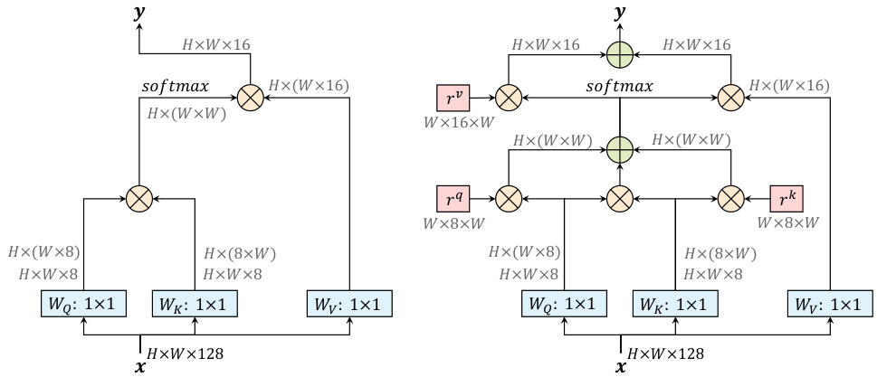
Fig. 1. A non-local block (left) vs. our position-sensitive axial-attention applied along the width-axis (right). “ $\bigotimes$ ” denotes matrix multiplication, and “ $\bigoplus$ ” denotes elementwise sum. The softmax is performed on the last axis. Blue boxes denote $1\times1$ convolutions, and red boxes denote relative positional encoding. The channels $d_{i n}=128$ , $d_{q}=8$ , and $d_{o u t}=16$ is what we use in the first stage of ResNet after ‘stem’
图 1: 非局部模块 (左) 与我们提出的沿宽度轴应用的位置敏感轴向注意力机制 (右) 对比。"$\bigotimes$"表示矩阵乘法,"$\bigoplus$"表示逐元素相加。softmax在最后一轴执行。蓝色框表示$1\times1$卷积,红色框表示相对位置编码。通道数$d_{in}=128$、$d_{q}=8$和$d_{out}=16$是我们在ResNet第一阶段"stem"后使用的配置
3.2 Axial-Attention
3.2 轴向注意力 (Axial-Attention)
The local constraint, proposed by the stand-alone self-attention models [68], significantly reduces the computational costs in vision tasks and enables building fully self-attention al model. However, such constraint sacrifices the global connection, making attention’s receptive field no larger than a depthwise convolution with the same kernel size. Additionally, the local self-attention, performed in local square regions, still has complexity quadratic to the region length, introducing another hyper-parameter to trade-off between performance and computation complexity. In this work, we propose to adopt axial-attention [42,33] in standalone self-attention, ensuring both global connection and efficient computation. Specifically, we first define an axial-attention layer on the width-axis of an image as simply a one dimensional position-sensitive self-attention, and use the similar definition for the height-axis. To be concrete, the axial-attention layer along the width-axis is defined as follows.
独立自注意力模型[68]提出的局部约束条件,显著降低了视觉任务中的计算成本,使构建全自注意力模型成为可能。然而这种约束牺牲了全局连接性,导致注意力的感受野不会超过同尺寸深度卷积的覆盖范围。此外,在局部方形区域执行的自注意力仍具有与区域长度平方相关的复杂度,这引入了另一个需要在性能与计算复杂度之间权衡的超参数。本文提出在独立自注意力中采用轴向注意力[42,33],既可保持全局连接又能实现高效计算。具体而言,我们首先将图像宽度轴上的轴向注意力层定义为简单的一维位置敏感自注意力,高度轴也采用类似定义。以宽度轴为例,轴向注意力层的定义如下。
$$
y_{o}=\sum_{p\in\mathcal{N}_ {1\times m}(o)}\mathrm{softmax}_ {p}(q_{o}^{T}k_{p}+q_{o}^{T}r_{p-o}^{q}+k_{p}^{T}r_{p-o}^{k})(v_{p}+r_{p-o}^{v})
$$
$$
y_{o}=\sum_{p\in\mathcal{N}_ {1\times m}(o)}\mathrm{softmax}_ {p}(q_{o}^{T}k_{p}+q_{o}^{T}r_{p-o}^{q}+k_{p}^{T}r_{p-o}^{k})(v_{p}+r_{p-o}^{v})
$$
One axial-attention layer propagates information along one particular axis. To capture global information, we employ two axial-attention layers consecutively for the height-axis and width-axis, respectively. Both of the axial-attention layers adopt the multi-head attention mechanism, as described above.
一个轴向注意力 (axial-attention) 层沿特定轴传播信息。为捕捉全局信息,我们依次采用两个轴向注意力层分别处理高度轴和宽度轴。这两个轴向注意力层均采用上文所述的多头注意力机制。
Axial-attention reduces the complexity to $\mathcal{O}(h w m)$ . This enables global receptive field, which is achieved by setting the span $m$ directly to the whole input features. Optionally, one could also use a fixed $m$ value, in order to reduce memory footprint on huge feature maps.
轴向注意力将复杂度降低至 $\mathcal{O}(h w m)$。这实现了全局感受野,通过直接将跨度 $m$ 设置为整个输入特征即可达成。此外,也可选择固定 $m$ 值以减少大型特征图的内存占用。
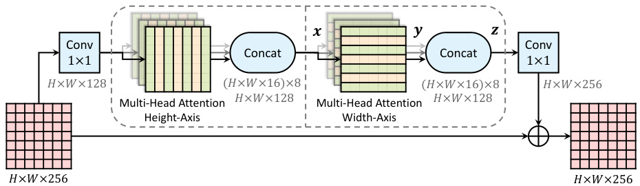
Fig. 2. An axial-attention block, which consists of two axial-attention layers operating along height- and width-axis sequentially. The channels $d_{i n}=128$ , $d_{o u t}=16$ is what we use in the first stage of ResNet after ‘stem’. We employ $N=8$ attention heads
图 2: 轴向注意力模块,由两个分别沿高度和宽度轴顺序操作的轴向注意力层组成。通道数 $d_{i n}=128$ 和 $d_{o u t}=16$ 是我们在ResNet第一阶段"stem"后使用的配置。我们采用了 $N=8$ 个注意力头。
Axial-ResNet: To transform a ResNet [32] to an Axial-ResNet, we replace the $3\times3$ convolution in the residual bottleneck block by two multi-head axialattention layers (one for height-axis and the other for width-axis). Optional striding is performed on each axis after the corresponding axial-attention layer. The two $1\times1$ convolutions are kept to shuffle the features. This forms our (residual) axial-attention block, as illustrated in Fig. 2, which is stacked multiple times to obtain Axial-ResNets. Note that we do not use a $1\times1$ convolution in-between the two axial-attention layers, since matrix multiplications $(W_{Q},W_{K},W_{V})$ follow immediately. Additionally, the stem (i.e., the first strided $7\times7$ convolution and $3\times3$ max-pooling) in the original ResNet is kept, resulting in a conv-stem model where convolution is used in the first layer and attention layers are used everywhere else. In conv-stem models, we set the span $m$ to the whole input from the first block, where the feature map is 56 $\times$ 56.
Axial-ResNet:要将ResNet [32]转换为Axial-ResNet,我们将残差瓶颈块中的$3\times3$卷积替换为两个多头轴向注意力层(分别对应高度轴和宽度轴)。在对应的轴向注意力层之后,每个轴上可选择进行跨步操作。保留两个$1\times1$卷积用于特征重排,由此构成如图2所示的(残差)轴向注意力块,通过多次堆叠该模块即可得到Axial-ResNet。需要注意的是,由于矩阵乘法$(W_{Q},W_{K},W_{V})$会紧随其后执行,因此我们不在两个轴向注意力层之间使用$1\times1$卷积。此外,保留了原始ResNet中的初始结构(即首个跨步$7\times7$卷积和$3\times3$最大池化),最终形成卷积初始模型——第一层使用卷积而其余层均采用注意力层。在卷积初始模型中,从首个模块开始将跨度$m$设置为整个输入(特征图尺寸为56$\times$56)。
In our experiments, we also build a full axial-attention model, called Full Axial-ResNet, which further applies axial-attention to the stem. Instead of designing a special spatially-varying attention stem [68], we simply stack three axial-attention bottleneck blocks. In addition, we adopt local constraints (i.e., a local $m\times m$ square region as in [68]) in the first few blocks of Full Axial-ResNets, in order to reduce computational cost.
在我们的实验中,我们还构建了一个完整的轴向注意力模型,称为Full Axial-ResNet,它进一步将轴向注意力应用于stem部分。我们没有设计特殊的空间变化注意力stem [68],而是简单地堆叠了三个轴向注意力瓶颈块。此外,我们在Full Axial-ResNet的前几个块中采用了局部约束(即类似于[68]中的局部 $m\times m$ 方形区域),以降低计算成本。
Axial-DeepLab: To further convert Axial-ResNet to Axial-DeepLab for segmentation tasks, we make several changes as discussed below.
轴向DeepLab:为了进一步将轴向ResNet转换为用于分割任务的轴向DeepLab,我们做了如下所述的几项改动。
Firstly, to extract dense feature maps, DeepLab [13] changes the stride and atrous rates of the last one or two stages in ResNet [32]. Similarly, we remove the stride of the last stage but we do not implement the ‘atrous’ attention module, since our axial-attention already captures global information for the whole input. In this work, we extract feature maps with output stride (i.e., the ratio of input resolution to the final backbone feature resolution) 16. We do not pursue output stride 8, since it is computationally expensive.
首先,为提取密集特征图,DeepLab [13] 调整了 ResNet [32] 最后一到两个阶段的步长和空洞率。类似地,我们去除了最后阶段的步长,但未实现"空洞"注意力模块,因为我们的轴向注意力已能捕获整个输入的全局信息。本工作中,我们提取输出步长(即输入分辨率与最终主干特征分辨率的比值)为16的特征图。未采用输出步长8的方案,因其计算成本较高。
Secondly, we do not adopt the atrous spatial pyramid pooling module (ASPP) [14,15], since our axial-attention block could also efficiently encode the multiscale or global information. We show in the experiments that our Axial-DeepLab without ASPP outperforms Panoptic-DeepLab [20] with and without ASPP.
其次,我们没有采用空洞空间金字塔池化模块 (ASPP) [14,15],因为我们的轴向注意力块也能高效编码多尺度或全局信息。实验表明,未使用ASPP的Axial-DeepLab在性能上优于使用及未使用ASPP的Panoptic-DeepLab [20]。
Lastly, following Panoptic-DeepLab [20], we adopt exactly the same stem [81] of three convolutions, dual decoders, and prediction heads. The heads produce semantic segmentation and class-agnostic instance segmentation, and they are merged by majority voting [93] to form the final panoptic segmentation.
最后,遵循Panoptic-DeepLab [20]的方法,我们采用了完全相同的三卷积主干网络 [81]、双解码器和预测头结构。这些预测头分别生成语义分割和类别无关的实例分割结果,并通过多数投票法 [93] 合并形成最终的全景分割输出。
In cases where the inputs are extremely large (e.g., 2177 $\times$ 2177) and memory is constrained, we resort to a large span $m=65$ in all our axial-attention blocks. Note that we do not consider the axial span as a hyper-parameter because it is already sufficient to cover long range or even global context on several datasets, and setting a smaller span does not significantly reduce M-Adds.
当输入尺寸极大(如2177 $\times$ 2177)且内存受限时,我们在所有轴向注意力(axial-attention)模块中采用大跨度$m=65$。需要注意的是,我们未将轴向跨度视为超参数,因为该值已足以覆盖多个数据集上的长距离甚至全局上下文,且设置更小的跨度不会显著减少乘加运算量(M-Adds)。
4 Experimental Results
4 实验结果
We conduct experiments on four large-scale datasets. We first report results with our Axial-ResNet on ImageNet [73]. We then convert the ImageNet pretrained Axial-ResNet to Axial-DeepLab, and report results on COCO [59], Mapillary Vistas [65], and Cityscapes [23] for panoptic segmentation, evaluated by panoptic quality (PQ) [48]. We also report average precision (AP) for instance segmentation, and mean IoU for semantic segmentation on Mapillary Vistas and Cityscapes. Our models are trained using TensorFlow [1] on 128 TPU cores for ImageNet and 32 cores for panoptic segmentation.
我们在四个大规模数据集上进行了实验。首先报告采用Axial-ResNet在ImageNet [73]上的结果,随后将ImageNet预训练的Axial-ResNet转换为Axial-DeepLab,并在COCO [59]、Mapillary Vistas [65]和Cityscapes [23]上报告全景分割 (panoptic segmentation) 结果,以全景质量 (PQ) [48]作为评估指标。同时报告Mapillary Vistas和Cityscapes的实例分割平均精度 (AP) 及语义分割平均交并比 (mIoU)。所有模型均使用TensorFlow [1]训练,其中ImageNet实验使用128个TPU核心,全景分割实验使用32个核心。
Training protocol: On ImageNet, we adopt the same training protocol as [68] for a fair comparison, except that we use batch size 512 for Full AxialResNets and 1024 for all other models, with learning rates scaled accordingly [30].
训练协议:在ImageNet上,我们采用与[68]相同的训练协议以确保公平比较,唯一区别是Full AxialResNets使用批量大小512,其他所有模型使用1024,并相应调整学习率[30]。
For panoptic segmentation, we strictly follow Panoptic-DeepLab [20], except using a linear warm up Radam [61] Lookahead [96] optimizer (with the same learning rate 0.001). All our results on panoptic segmentation use this setting. We note this change does not improve the results, but smooths our training curves. Panoptic-DeepLab yields similar result in this setting.
在全景分割任务中,我们严格遵循Panoptic-DeepLab [20]的设定,仅将优化器改为线性热身的Radam [61] Lookahead [96] (学习率保持0.001不变)。所有全景分割实验结果均采用该配置。需要说明的是,这一调整虽未提升指标,但使训练曲线更平滑。在此设置下,Panoptic-DeepLab保持了相近的性能表现。
4.1 ImageNet
4.1 ImageNet
For ImageNet, we build Axial-ResNet-L from ResNet-50 [32]. In detail, we set $d_{i n}=128$ , $d_{o u t}=2d_{q}=16$ for the first stage after the ‘stem’. We double them when spatial resolution is reduced by a factor of 2 [79]. Additionally, we multiply all the channels [36,74,35] by 0.5, 0.75, and 2, resulting in AxialResNet-{S, M, XL}, respectively. Finally, Stand-Alone Axial-ResNets are further generated by replacing the ‘stem’ with three axial-attention blocks where the first block has stride 2. Due to the computational cost introduced by the early layers, we set the axial span $m=15$ in all blocks of Stand-Alone Axial-ResNets. We always use $N~=~8$ heads [68]. In order to avoid careful initialization of $W_{Q},W_{K},W_{V},r^{q},r^{k},r^{v}$ , we use batch normalization s [43] in all attention layers. Tab. $^{1}$ summarizes our ImageNet results. The baselines ResNet-50 [32] (done by [68]) and Conv-Stem $^+$ Attention [68] are also listed. In the conv-stem setting, adding BN to attention layers of [68] slightly improves the performance by 0.3%.
对于ImageNet数据集,我们基于ResNet-50 [32]构建了Axial-ResNet-L。具体而言,在"stem"层后的第一阶段设置$d_{in}=128$、$d_{out}=2d_{q}=16$。当空间分辨率降低为1/2时 [79],我们将这些值翻倍。此外,将所有通道数 [36,74,35]分别乘以0.5、0.75和2,得到AxialResNet-{S, M, XL}变体。最终,通过将"stem"替换为三个轴向注意力块(其中第一个块的步长为2)生成独立式Axial-ResNet。由于早期层引入的计算成本,我们在独立式Axial-ResNet所有块中设置轴向跨度$m=15$。始终采用$N~=~8$个头 [68]。为避免精心初始化$W_{Q},W_{K},W_{V},r^{q},r^{k},r^{v}$,我们在所有注意力层使用批量归一化 [43]。表$^{1}$汇总了ImageNet实验结果,同时列出基线模型ResNet-50 [32](由[68]实现)和Conv-Stem$^+$Attention [68]。在卷积stem设置中,为[68]的注意力层添加BN可使性能微升0.3%。
Table 1. ImageNet validation set results. BN: Use batch normalization s in attention layers. PS: Our position-sensitive self-attention. Full: Stand-alone self-attention models without spatial convolutions
| Method | BN | PS | Full | Params | M-Adds | Top-1 |
| Conv-Stem methods | ||||||
| ResNet-50 [32,68] Conv-Stem + Attention [68] | 25.6M 18.0M | 4.1B 3.5B | 76.9 77.4 | |||
| Conv-Stem+Attention | 18.0M | 3.5B | 77.7 | |||
| Conv-Stem + PS-Attention Conv-Stem + Axial-Attention | 18.0M 12.4M | 3.7B 2.8B | 78.1 77.5 | |||
| Fully self-attentional methods | ||||||
| LR-Net-50 [38] | 23.3M | 4.3B | 77.3 | |||
| Full Attention [68] | 18.0M | 3.6B | 77.6 | |||
| FullAxial-Attention | 12.5M | 3.3B | 78.1 | |||
表 1: ImageNet验证集结果。BN: 在注意力层使用批量归一化。PS: 我们的位置敏感自注意力。Full: 不含空间卷积的独立自注意力模型
| 方法 | BN | PS | Full | 参数量 | M-Adds | Top-1 |
|---|---|---|---|---|---|---|
| Conv-Stem方法 | ||||||
| ResNet-50 [32,68] Conv-Stem + Attention [68] | 25.6M 18.0M | 4.1B 3.5B | 76.9 77.4 | |||
| Conv-Stem+Attention | 18.0M | 3.5B | 77.7 | |||
| Conv-Stem + PS-Attention Conv-Stem + Axial-Attention | 18.0M 12.4M | 3.7B 2.8B | 78.1 77.5 | |||
| 纯自注意力方法 | ||||||
| LR-Net-50 [38] | 23.3M | 4.3B | 77.3 | |||
| Full Attention [68] | 18.0M | 3.6B | 77.6 | |||
| FullAxial-Attention | 12.5M | 3.3B | 78.1 |
Our proposed position-sensitive self-attention (Conv-Stem $^+$ PS-Attention) further improves the performance by $0.4%$ at the cost of extra marginal computation. Our Conv-Stem $^+$ Axial-Attention performs on par with Conv-Stem $^+$ Attention [68] while being more parameter- and computation-efficient. When comparing with other full self-attention models, our Full Axial-Attention outperforms Full Attention [68] by $0.5%$ , while being $1.44\times$ more parameter-efficient and 1.09 $\times$ more computation-efficient.
我们提出的位置敏感自注意力机制 (Conv-Stem $^+$ PS-Attention) 以额外边际计算为代价,将性能进一步提升了 $0.4%$。我们的 Conv-Stem $^+$ Axial-Attention 与 Conv-Stem $^+$ Attention [68] 性能相当,同时具有更高的参数和计算效率。与其他全自注意力模型相比,我们的 Full Axial-Attention 比 Full Attention [68] 高出 $0.5%$,同时参数效率提升 $1.44\times$,计算效率提升 $1.09\times$。
Following [68], we experiment with different network widths (i.e., AxialResNets-{S,M,L,XL}), exploring the trade-off between accuracy, model parameters, and computational cost (in terms of M-Adds). As shown in Fig. 3, our proposed Conv-Stem $^+$ PS-Attention and Conv-Stem $^+$ Axial-Attention already outperforms ResNet-50 [32,68] and attention models [68] (both Conv-Stem $^+$ Attention, and Full Attention) at all settings. Our Full Axial-Attention further attains the best accuracy-parameter and accuracy-complexity trade-offs.
遵循[68],我们尝试了不同的网络宽度(即AxialResNets-{S,M,L,XL}),探索准确率、模型参数和计算成本(以M-Adds衡量)之间的权衡。如图3所示,我们提出的Conv-Stem$^+$PS-Attention和Conv-Stem$^+$Axial-Attention在所有设置下均优于ResNet-50[32,68]和注意力模型[68](包括Conv-Stem$^+$Attention和Full Attention)。我们的Full Axial-Attention进一步实现了最佳的准确率-参数和准确率-复杂度权衡。
4.2 COCO
4.2 COCO
The ImageNet pretrained Axial-ResNet model variants (with different channels) are then converted to Axial-DeepLab model variant for panoptic segmentation tasks. We first demonstrate the effectiveness of our Axial-DeepLab on the challenging COCO dataset [59], which contains objects with various scales (from less than $32\times32$ to larger than $96\times96$ ).
ImageNet预训练的Axial-ResNet模型变体(不同通道数)随后被转换为用于全景分割任务的Axial-DeepLab模型变体。我们首先在具有挑战性的COCO数据集[59]上验证Axial-DeepLab的有效性,该数据集包含多种尺度的物体(从小于$32\times32$到大于$96\times96$)。
Val set: In Tab. 2, we report our validation set results and compare with other bottom-up panoptic segmentation methods, since our method also belongs to the bottom-up family. As shown in the table, our single-scale Axial-DeepLab-S outperforms DeeperLab [93] by 8% PQ, multi-scale SSAP [29] by 5.3% PQ, and single-scale Panoptic-DeepLab by 2.1% PQ. Interestingly, our single-scale AxialDeepLab-S also outperforms multi-scale Panoptic-DeepLab by 0.6% PQ while being $\mathbf{3.8\times}$ parameter-efficient and $\mathbf{27\times}$ computation-efficient (in M-Adds). Increasing the backbone capacity (via large channels) continuously improves the performance. Specifically, our multi-scale Axial-DeepLab-L attains $43.9%$ PQ, outperforming Panoptic-DeepLab [20] by 2.7% PQ.
验证集:在表2中,我们报告了验证集结果,并与其他自底向上的全景分割方法进行对比,因为我们的方法也属于自底向上流派。如表所示,我们的单尺度Axial-DeepLab-S以8% PQ优势超越DeeperLab[93],以5.3% PQ优势超越多尺度SSAP[29],以2.1% PQ优势超越单尺度Panoptic-DeepLab。值得注意的是,我们的单尺度Axial-DeepLab-S还以0.6% PQ优势超越多尺度Panoptic-DeepLab,同时具有$\mathbf{3.8\times}$参数效率和$\mathbf{27\times}$计算效率(以M-Adds衡量)。通过增大通道数来提升主干网络容量可持续改善性能。具体而言,我们的多尺度Axial-DeepLab-L达到$43.9%$ PQ,以2.7% PQ优势超越Panoptic-DeepLab[20]。
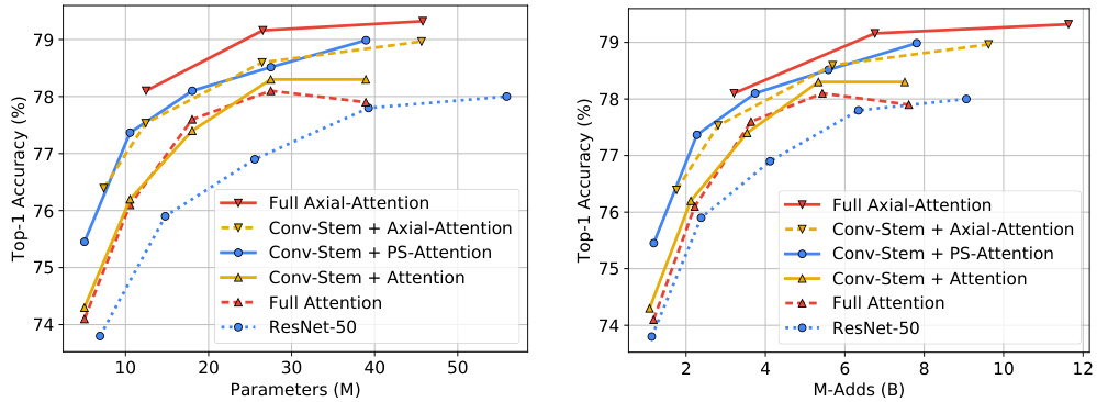
Fig. 3. Comparing parameters and M-Adds against accuracy on ImageNet classification. Our position-sensitive self-attention (Conv-Stem $+$ PS-Attention) and axialattention (Conv-Stem $+$ Axial-Attention) consistently outperform ResNet-50 [32,68] and attention models [68] (both Conv-Stem $^+$ Attention, and Full Attention), across a range of network widths (i.e., different channels). Our Full Axial-Attention works the best in terms of both parameters and M-Adds
图 3: 在ImageNet分类任务上比较参数量和M-Adds与准确率的关系。我们的位置敏感自注意力(Conv-Stem $+$ PS-Attention)和轴向注意力(Conv-Stem $+$ Axial-Attention)在不同网络宽度(即不同通道数)下均优于ResNet-50 [32,68]和注意力模型[68](包括Conv-Stem $^+$ Attention和Full Attention)。我们的Full Axial-Attention在参数量和M-Adds方面表现最佳
Table 2. COCO val set. MS: Multi-scale inputs
| Method | Backbone | MS | Params | M-Adds | PQ | PQ Th | PQSt |
| DeeperLab [93] SSAP [29] Panoptic-DeepLab 20] Panoptic-DeepLab 20 | Xception-71 ResNet-101 Xception-71 | 46.7M | 274.0B | 33.8 36.5 39.7 | 43.9 | 33.2 | |
| Axial-DeepLab-S | Axial-ResNet-S | 12.1M | 110.4B | 41.8 | 46.1 | 35.2 | |
| Axial-DeepLab-M | Axial-ResNet-M | 25.9M | 209.9B | 42.9 | 47.6 | 35.8 | |
| Axial-DeepLab-L | Axial-ResNet-L | 44.9M | 343.9B | 43.4 | 48.5 | 35.6 | |
| Axial-DeepLab-L | Axial-ResNet-L | 44.9M | 3867.7B | 43.9 | 48.6 | ||
| 36.8 |
表 2. COCO验证集。MS: 多尺度输入
| 方法 | 骨干网络 | MS | 参数量 | M-Adds | PQ | PQ Th | PQSt |
|---|---|---|---|---|---|---|---|
| DeeperLab [93] SSAP [29] Panoptic-DeepLab [20] Panoptic-DeepLab [20] | Xception-71 ResNet-101 Xception-71 | 46.7M | 274.0B | 33.8 36.5 39.7 | 43.9 | 33.2 | |
| Axial-DeepLab-S | Axial-ResNet-S | 12.1M | 110.4B | 41.8 | 46.1 | 35.2 | |
| Axial-DeepLab-M | Axial-ResNet-M | 25.9M | 209.9B | 42.9 | 47.6 | 35.8 | |
| Axial-DeepLab-L | Axial-ResNet-L | 44.9M | 343.9B | 43.4 | 48.5 | 35.6 | |
| Axial-DeepLab-L | Axial-ResNet-L | 44.9M | 3867.7B | 43.9 | 48.6 | ||
| 36.8 |
Test-dev set: As shown in Tab. 3, our Axial-DeepLab variants show consistent improvements with larger backbones. Our multi-scale Axial-DeepLab-L attains the performance of $44.2%$ PQ, outperforming DeeperLab [93] by $9.9%$ PQ, SSAP [29] by $7.3%$ PQ, and Panoptic-DeepLab [20] by 2.8% PQ, setting a new state-of-the-art among bottom-up approaches. We also list several topperforming methods adopting the top-down approaches in the table for reference.
测试开发集 (Test-dev set): 如表 3 所示,我们的 Axial-DeepLab 变体随着主干网络增大展现出持续性能提升。多尺度 Axial-DeepLab-L 取得了 44.2% PQ 的优异表现,比 DeeperLab [93] 高出 9.9% PQ,超越 SSAP [29] 7.3% PQ,并领先 Panoptic-DeepLab [20] 2.8% PQ,在自底向上方法中创造了新的最先进水平。表中还列出了若干采用自顶向下方法的顶尖算法作为参考。
Scale Stress Test: In order to verify that our model learns long range interactions, we perform a scale stress test besides standard testing. In the stress test, we train Panoptic-DeepLab (X-71) and our Axial-DeepLab-L with the standard setting, but test them on out-of-distribution resolutions (i.e., resize the input to different resolutions). Fig. 4 summarizes our relative improvements over Panoptic-DeepLab on PQ, PQ (thing) and PQ (stuff). When tested on huge images, Axial-DeepLab shows large gain (30%), demonstrating that it encodes long range relations better than convolutions. Besides, Axial-DeepLab improves 40% on small images, showing that axial-attention is more robust to scale variations.
规模压力测试:为验证模型学习长程交互的能力,我们在标准测试外进行了规模压力测试。该测试中,我们以标准设置训练Panoptic-DeepLab (X-71)和Axial-DeepLab-L,但在分布外分辨率(即调整输入至不同分辨率)下测试它们。图4汇总了我们在PQ、PQ(thing)和PQ(stuff)指标上相对于Panoptic-DeepLab的相对改进。当测试超大图像时,Axial-DeepLab显示出30%的大幅提升,证明其比卷积方法更能编码长程关系。此外,Axial-DeepLab在小图像上提升40%,表明轴向注意力(axial-attention)对尺度变化更具鲁棒性。
Table 3. COCO test-dev set. MS: Multi-scale inputs
| Method | Backbone | MS | PQ | PQTh | PQSt |
| Top-down panoptic segmentation methods | |||||
| TASCNet [52] Panoptic-FPN [47] AdaptIS [80] AUNet [55] UPSNet [91] Li et al. [53] SpatialFlow [17] | ResNet-50 ResNet-101 ResNeXt-101 ResNeXt-152 DCN-101 [24] DCN-101 [24] | 40.7 40.9 42.8 46.5 46.6 47.2 | 47.0 48.3 53.2 55.8 53.2 53.5 | 31.0 29.7 36.7 32.5 36.7 | |
| SOGNet [94] DCN-101 [24] 47.8 Bottom-up panoptic segmentation methods | |||||
| DeeperLab [93] SSAP [29] Panoptic-DeepLab [20] | Xception-71 ResNet-101 Xception-71 | 34.3 36.9 41.4 | 37.5 40.1 45.1 | 29.6 32.0 | |
| Axial-DeepLab-S Axial-DeepLab-M Axial-DeepLab-L Axial-DeepLab-L | Axial-ResNet-S Axial-ResNet-M Axial-ResNet-L Axial-ResNet-L | 42.2 43.2 43.6 44.2 | 46.5 48.1 48.9 49.2 | 35.7 35.9 35.6 36.8 | |
表 3. COCO test-dev 集。MS: 多尺度输入
| 方法 | 主干网络 | MS | PQ | PQTh | PQSt |
|---|---|---|---|---|---|
| 自上而下的全景分割方法 | |||||
| TASCNet [52] Panoptic-FPN [47] AdaptIS [80] AUNet [55] UPSNet [91] Li et al. [53] SpatialFlow [17] | ResNet-50 ResNet-101 ResNeXt-101 ResNeXt-152 DCN-101 [24] DCN-101 [24] | 40.7 40.9 42.8 46.5 46.6 47.2 | 47.0 48.3 53.2 55.8 53.2 53.5 | 31.0 29.7 36.7 32.5 36.7 | |
| SOGNet [94] | DCN-101 [24] | 47.8 | |||
| 自下而上的全景分割方法 | |||||
| DeeperLab [93] SSAP [29] Panoptic-DeepLab [20] | Xception-71 ResNet-101 Xception-71 | 34.3 36.9 41.4 | 37.5 40.1 45.1 | 29.6 32.0 | |
| Axial-DeepLab-S Axial-DeepLab-M Axial-DeepLab-L Axial-DeepLab-L | Axial-ResNet-S Axial-ResNet-M Axial-ResNet-L Axial-ResNet-L | 42.2 43.2 43.6 44.2 | 46.5 48.1 48.9 49.2 | 35.7 35.9 35.6 36.8 |
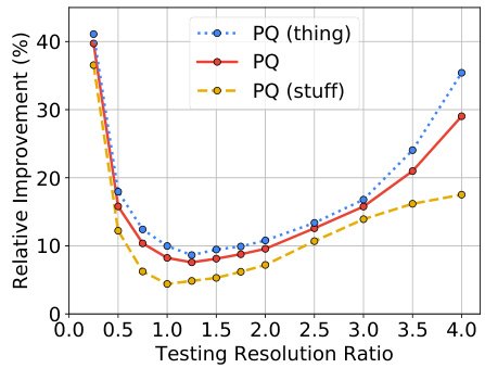
Fig. 4. Scale stress test on COCO val set. Axial-DeepLab gains the most when tested on extreme resolutions. On the x-axis, ratio 4.0 means inference with resolution 4097 $\times$ 4097
图 4: COCO验证集上的尺度压力测试。Axial-DeepLab在极端分辨率下测试时收益最大。x轴上,比例4.0表示使用4097 $\times$ 4097分辨率进行推理
4.3 Mapillary Vistas
4.3 Mapillary Vistas
Table 4. Mapillary Vistas validation set. MS: Multi-scale inputs
| Method | MS|Params M-Adds|PQ PQTh PQst AP mIoU | ||||||||||
| Top-down panoptic segmentation methods | |||||||||||
| TASCNet [52] | |||||||||||
| TASCNet [52] | 32.6 34.3 | 31.1 34.8 | 34.4 18.5 33.6 | 20.4 | |||||||
| 35.9 | 31.5 | 41.9 | |||||||||
| AdaptIS [80] | 37.7 | 33.8 | |||||||||
| Seamless [71] | 42.9 | 16.4 | 50.4 | ||||||||
| Bottom-up panoptic segmentation methods | |||||||||||
| DeeperLab [93] | |||||||||||
| Panoptic-DeepLab (Xception-71 [21,72]) [20] | 46.7M | 1.24T | 32.0 37.7 | 30.4 | 47.414.9 | 55.4 | |||||
| Panoptic-DeepLab o (Xception-71 [21,72]) [20] | 46.7M | 31.35T | 40.3 | 33.5 | 49.3 | 17.2 | 56.8 | ||||
| Panoptic-DeepLab (HRNet-W48 [86])[20] | 71.7M | 58.47T | 39.3 | 17.2 | 55.4 | ||||||
| Panoptic-DeepLab (Auto-XL++ [60]) [20] | 72.2M | 60.55T | 40.3 | 16.9 | 57.6 | ||||||
| Axial-DeepLab-L Axial-DeepLab-L | 44.9M | 44.9M 1.55T 39.35T | 40.1 | 41.1 | 32.7 33.4 | 49.8 51.3 17.2 | 16.7 | 57.6 58.4 | |||
表 4. Mapillary Vistas 验证集。MS: 多尺度输入
| 方法 | MS | Params M-Adds | PQ | PQTh | PQst | AP | mIoU |
|---|---|---|---|---|---|---|---|
| 自上而下的全景分割方法 | |||||||
| TASCNet [52] | 32.6 | 34.3 | 31.1 | 34.8 | 34.4 | ||
| TASCNet [52] | 35.9 | 31.5 | 41.9 | ||||
| AdaptIS [80] | 37.7 | 33.8 | |||||
| Seamless [71] | 42.9 | 16.4 | 50.4 | ||||
| 自下而上的全景分割方法 | |||||||
| DeeperLab [93] | |||||||
| Panoptic-DeepLab (Xception-71 [21,72]) [20] | 46.7M | 1.24T | 32.0 | 37.7 | 30.4 | 47.4 | 55.4 |
| Panoptic-DeepLab o (Xception-71 [21,72]) [20] | 46.7M | 31.35T | 40.3 | 33.5 | 49.3 | 17.2 | 56.8 |
| Panoptic-DeepLab (HRNet-W48 [86]) [20] | 71.7M | 58.47T | 39.3 | 17.2 | 55.4 | ||
| Panoptic-DeepLab (Auto-XL++ [60]) [20] | 72.2M | 60.55T | 40.3 | 16.9 | 57.6 | ||
| Axial-DeepLab-L | 44.9M | 1.55T | 40.1 | 32.7 | 49.8 | 17.2 | 57.6 |
| Axial-DeepLab-L | 44.9M | 39.35T | 41.1 | 33.4 | 51.3 | 16.7 | 58.4 |
Val set: As shown in Tab. 4, our Axial-DeepLab-L outperforms all the stateof-the-art methods in both single-scale and multi-scale cases. Our single-scale Axial-DeepLab-L performs $2.4%$ PQ better than the previous best single-scale Panoptic-DeepLab (X-71) [20]. In multi-scale setting, our lightweight AxialDeepLab-L performs better than Panoptic-DeepLab (Auto-DeepLab-XL ${++}$ ), not only on panoptic segmentation (0.8% PQ) and instance segmentation ( $0.3%$ AP), but also on semantic segmentation (0.8% mIoU), the task that AutoDeepLab [60] was searched for. Additionally, to the best of our knowledge, our Axial-DeepLab-L attains the best single-model semantic segmentation result.
验证集:如表 4 所示,我们的 Axial-DeepLab-L 在单尺度和多尺度情况下均优于所有最先进方法。单尺度 Axial-DeepLab-L 的 PQ 值比之前最佳单尺度 Panoptic-DeepLab (X-71) [20] 高出 2.4%。在多尺度设置中,我们的轻量级 Axial-DeepLab-L 不仅在全景分割 (0.8% PQ) 和实例分割 (0.3% AP) 上优于 Panoptic-DeepLab (Auto-DeepLab-XL++),在 AutoDeepLab [60] 所优化的语义分割任务 (0.8% mIoU) 上也表现更优。此外,据我们所知,Axial-DeepLab-L 实现了目前最佳的单模型语义分割结果。
4.4 Cityscapes
4.4 Cityscapes
Val set: In Tab. 5 (a), we report our Cityscapes validation set results. Without using extra data (i.e., only Cityscapes fine annotation), our Axial-DeepLab achieves $65.1%$ PQ, which is $1%$ better than the current best bottom-up PanopticDeepLab [20] and $3.1%$ better than proposal-based AdaptIS [80]. When using extra data (e.g., Mapillary Vistas [65]), our multi-scale Axial-DeepLab-XL attains $68.5%$ PQ, $1.5%$ better than Panoptic-DeepLab [20] and $3.5%$ better than Seamless [71]. Our instance segmentation and semantic segmentation results are respectively $1.7%$ and $1.5%$ better than Panoptic-DeepLab [20].
验证集:在表5(a)中,我们报告了Cityscapes验证集的结果。在不使用额外数据(即仅使用Cityscapes精细标注)的情况下,我们的Axial-DeepLab达到了65.1% PQ,比当前最佳自底向上方法PanopticDeepLab [20]高出1%,比基于提案的AdaptIS [80]高出3.1%。当使用额外数据(如Mapillary Vistas [65])时,我们的多尺度Axial-DeepLab-XL获得了68.5% PQ,比Panoptic-DeepLab [20]高1.5%,比Seamless [71]高3.5%。我们的实例分割和语义分割结果分别比Panoptic-DeepLab [20]高出1.7%和1.5%。
Test set: Tab. 5 (b) shows our test set results. Without extra data, AxialDeepLab-XL attains $62.8%$ PQ, setting a new state-of-the-art result. Our model further achieves $66.6%$ PQ, $39.6%$ AP, and $84.1%$ mIoU with Mapillary Vistas pre training. Note that Panoptic-DeepLab [20] adopts the trick of output stride 8 during inference on test set, making their M-Adds comparable to our XL models.
测试集:表5 (b) 展示了我们的测试集结果。在不使用额外数据的情况下,AxialDeepLab-XL达到了62.8% PQ,创造了新的最优性能。通过Mapillary Vistas预训练后,我们的模型进一步实现了66.6% PQ、39.6% AP和84.1% mIoU。需要注意的是,Panoptic-DeepLab [20]在测试集推理时采用了输出步长8的技巧,使其M-Adds与我们的XL模型具有可比性。
4.5 Ablation Studies
4.5 消融实验
We perform ablation studies on Cityscapes validation set.
我们在Cityscapes验证集上进行消融实验。
Table 5. Cityscapes val set and test set. MS: Multi-scale inputs. C: Cityscapes coarse annotation. V: Cityscapes video. MV: Mapillary Vistas
| Method | ExtraData|MSPQ | AP mIoU |
| AdaptIS [80] | 62.0 36.3 79.2 | |
| SSAP [29] Panoptic-DeepLab[20] Panoptic-DeepLab[20] | 61.1 37.3 = 63.0 35.3 80.5 64.1 38.5 81.5 | |
| Axial-DeepLab-L Axial-DeepLab-L Axial-DeepLab-XL Axial-DeepLab-XL | 63.9 935.8 81.0 64.7 37.9 81.5 64.4 36.7 80.6 65.1 39.0 81.1 | |
| SpatialFlow [17] Seamless [71] | COCO MV | 62.5 65.0 80.7 |
| Panoptic-DeepLab [20] Panoptic-DeepLab [20] | MV MV | 65.3 38.8 82.5 67.0 42.5 83.1 |
| Axial-DeepLab-L Axial-DeepLab-L Axial-DeepLab-XL Axial-DeepLab-XL | MV MV MV MV | 66.5 40.2 83.2 67.7 42.9 83.8 67.8 41.9 84.2 68.544.284.6 |
表 5: Cityscapes验证集和测试集。MS: 多尺度输入。C: Cityscapes粗标注。V: Cityscapes视频。MV: Mapillary Vistas
| 方法 | 额外数据 | MSPQ | AP mIoU |
|---|---|---|---|
| AdaptIS [80] | 62.0 36.3 79.2 | ||
| SSAP [29] Panoptic-DeepLab[20] Panoptic-DeepLab[20] | 61.1 37.3 = 63.0 35.3 80.5 64.1 38.5 81.5 | ||
| Axial-DeepLab-L Axial-DeepLab-L Axial-DeepLab-XL Axial-DeepLab-XL | 63.9 935.8 81.0 64.7 37.9 81.5 64.4 36.7 80.6 65.1 39.0 81.1 | ||
| SpatialFlow [17] Seamless [71] | COCO MV | 62.5 65.0 80.7 | |
| Panoptic-DeepLab [20] Panoptic-DeepLab [20] | MV MV | 65.3 38.8 82.5 67.0 42.5 83.1 | |
| Axial-DeepLab-L Axial-DeepLab-L Axial-DeepLab-XL Axial-DeepLab-XL | MV MV MV MV | 66.5 40.2 83.2 67.7 42.9 83.8 67.8 41.9 84.2 68.544.284.6 |
(a) Cityscapes validation set (b) Cityscapes test set
| Method | ExtraDatalPQAPmIoU | ||
| GFF-Net [54] Zhu et al. [101] AdaptIS [80] | C,V, MV | 32.5 | 82.3 83.5 |
| UPSNet [91] PANet [62] PolyTransform [57] | COCO COCO COCO | 33.0 36.4 40.1 | |
| SSAP [29] Li et al. [53] Panoptic-DeepLab[20] TASCNet [52] Seamless [71] Li et al. [53] Panoptic-DeepLab[20] | COCO MV COCO MV | 58.9 32.7 61.0 = 62.3 34.6 60.7 62.6 = 63.3 65.5 39.0 | 79.4 84.2 |
| Axial-DeepLab-L Axial-DeepLab-XL Axial-DeepLab-L Axial-DeepLab-XL | MV MV | 62.7 33.3 62.8 34.0 65.6 38.1 66.6 39.6 84.1 | 79.5 79.9 83.1 |
(a) Cityscapes验证集
(b) Cityscapes测试集
| 方法 | 额外数据 | PQ | AP | mIoU |
|---|---|---|---|---|
| GFF-Net [54] Zhu et al. [101] AdaptIS [80] | C,V,MV | 32.5 | - | 82.3 83.5 |
| UPSNet [91] PANet [62] PolyTransform [57] | COCO COCO COCO | 33.0 36.4 40.1 | - | - |
| SSAP [29] Li et al. [53] Panoptic-DeepLab[20] TASCNet [52] Seamless [71] Li et al. [53] Panoptic-DeepLab[20] | COCO MV COCO MV | 58.9 32.7 61.0 = 62.3 34.6 60.7 62.6 = 63.3 65.5 39.0 | - | 79.4 84.2 |
| Axial-DeepLab-L Axial-DeepLab-XL Axial-DeepLab-L Axial-DeepLab-XL | MV MV | 62.7 33.3 62.8 34.0 65.6 38.1 66.6 39.6 84.1 | - | 79.5 79.9 83.1 |
Table 6. Ablating self-attention variants on Cityscapes val set. ASPP: Atrous spatial pyramid pooling. PS: Our position-sensitive self-attention
| Backbone | ASPP | PS | Params | M-Adds | PQ | AP | mIoU |
| ResNet-50 [32] (our impl.) | 24.8M 30.0M | 374.8B 390.0B | 58.1 59.8 | 30.0 32.6 | 73.3 77.8 | ||
| ResNet-50 32 ] (our impl.) Attention [68] (our impl.) | 17.3M | 317.7B | 58.7 | 31.9 | 75.8 | ||
| Attention [68] (our impl.) | 22.5M | 332.9B | 60.9 | 30.0 | 78.2 | ||
| 17.3M | 326.7B | 59.9 | 32.2 | 76.3 | |||
| PS-Attention PS-Attention | 22.5M | 341.9B | 61.5 | 33.1 | 79.1 | ||
| Axial-DeepLab-S | 12.1M | 220.8B | 62.6 | 34.9 | 80.5 | ||
| Axial-DeepLab-M | 25.9M | 419.6B | 63.1 | 35.6 | 80.3 | ||
| Axial-DeepLab-L | 44.9M | 687.4B | 63.9 | 35.8 | 81.0 | ||
| Axial-DeepLab-XL | 173.0M | 2446.8B | 64.4 | 36.7 | 80.6 |
表 6: 在Cityscapes验证集上消融自注意力变体的结果。ASPP: 空洞空间金字塔池化。PS: 我们的位置敏感自注意力
| Backbone | ASPP | PS | Params | M-Adds | PQ | AP | mIoU |
|---|---|---|---|---|---|---|---|
| ResNet-50 [32] (our impl.) | 24.8M 30.0M | 374.8B 390.0B | 58.1 59.8 | 30.0 32.6 | 73.3 77.8 | ||
| ResNet-50 [32] (our impl.) Attention [68] (our impl.) | 17.3M | 317.7B | 58.7 | 31.9 | 75.8 | ||
| Attention [68] (our impl.) | 22.5M | 332.9B | 60.9 | 30.0 | 78.2 | ||
| 17.3M | 326.7B | 59.9 | 32.2 | 76.3 | |||
| PS-Attention | 22.5M | 341.9B | 61.5 | 33.1 | 79.1 | ||
| Axial-DeepLab-S | 12.1M | 220.8B | 62.6 | 34.9 | 80.5 | ||
| Axial-DeepLab-M | 25.9M | 419.6B | 63.1 | 35.6 | 80.3 | ||
| Axial-DeepLab-L | 44.9M | 687.4B | 63.9 | 35.8 | 81.0 | ||
| Axial-DeepLab-XL | 173.0M | 2446.8B | 64.4 | 36.7 | 80.6 |
Importance of Position-Sensitivity and Axial-Attention: In Tab. 1, we experiment with attention models on ImageNet. In this ablation study, we transfer them to Cityscapes segmentation tasks. As shown in Tab. 6, all variants outperform ResNet-50 [32]. Position-sensitive attention performs better than previous self-attention [68], which aligns with ImageNet results in Tab. 1. However, employing axial-attention, which is on-par with position-sensitive attention on ImageNet, gives more than $1%$ boosts on all three segmentation tasks (in PQ, AP, and mIoU), without ASPP, and with fewer parameters and M-Adds, suggesting that the ability to encode long range context of axial-attention significantly improves the performance on segmentation tasks with large input images.
位置敏感性与轴向注意力机制的重要性:在表 1中,我们在ImageNet上对注意力模型进行了实验。在这项消融研究中,我们将这些模型迁移到Cityscapes分割任务中。如表 6所示,所有变体均优于ResNet-50 [32]。位置敏感注意力的表现优于之前的自注意力机制 [68],这与表 1中的ImageNet结果一致。然而,采用轴向注意力机制(在ImageNet上与位置敏感注意力表现相当)时,无需ASPP模块且参数量和M-Adds更少的情况下,三项分割任务(PQ、AP和mIoU)均获得超过$1%$的性能提升,这表明轴向注意力机制对长距离上下文关系的编码能力显著提升了大幅面输入图像分割任务的性能。
Table 7. Varying axial-attention span on Cityscapes val set
| Backbone | Span | Params | M-Adds | PQ | AP | mIoU |
| ResNet-101 | 43.8M | 530.0B | 59.9 | 31.9 | 74.6 | |
| Axial-ResNet-L | 5×5 | 44.9M | 617.4B | 59.1 | 31.3 | 74.5 |
| Axial-ResNet-L | 9x9 | 44.9M | 622.1B | 61.2 | 31.1 | 77.6 |
| Axial-ResNet-L | 17 × 17 | 44.9M | 631.5B | 62.8 | 34.0 | 79.5 |
| Axial-ResNet-L | 33×33 | 44.9M | 650.2B | 63.8 | 35.9 | 80.2 |
| Axial-ResNet-L | 65×65 | 44.9M | 687.4B | 64.2 | 36.3 | 80.6 |
表 7. Cityscapes验证集上轴向注意力范围的变化
| Backbone | Span | Params | M-Adds | PQ | AP | mIoU |
|---|---|---|---|---|---|---|
| ResNet-101 | 43.8M | 530.0B | 59.9 | 31.9 | 74.6 | |
| Axial-ResNet-L | 5×5 | 44.9M | 617.4B | 59.1 | 31.3 | 74.5 |
| Axial-ResNet-L | 9×9 | 44.9M | 622.1B | 61.2 | 31.1 | 77.6 |
| Axial-ResNet-L | 17×17 | 44.9M | 631.5B | 62.8 | 34.0 | 79.5 |
| Axial-ResNet-L | 33×33 | 44.9M | 650.2B | 63.8 | 35.9 | 80.2 |
| Axial-ResNet-L | 65×65 | 44.9M | 687.4B | 64.2 | 36.3 | 80.6 |
Importance of Axial-Attention Span: In Tab. 7, we vary the span $m$ (i.e., spatial extent of local regions in an axial block), without ASPP. We observe that a larger span consistently improves the performance at marginal costs.
轴向注意力跨度的重要性:在表7中,我们改变了跨度$m$(即轴向块中局部区域的空间范围),未使用ASPP。我们观察到,更大的跨度能以边际成本持续提升性能。
5 Conclusion and Discussion
5 结论与讨论
In this work, we have shown the effectiveness of proposed position-sensitive axialattention on image classification and segmentation tasks. On ImageNet, our Axial-ResNet, formed by stacking axial-attention blocks, achieves state-of-theart results among stand-alone self-attention models. We further convert AxialResNet to Axial-DeepLab for bottom-up segmentation tasks, and also show state-of-the-art performance on several benchmarks, including COCO, Mapillary Vistas, and Cityscapes. We hope our promising results could establish that axial-attention is an effective building block for modern computer vision models.
在本研究中,我们证明了所提出的位置敏感轴向注意力(position-sensitive axial attention)在图像分类和分割任务中的有效性。在ImageNet上,通过堆叠轴向注意力模块构建的Axial-ResNet,在独立自注意力模型中取得了最先进的结果。我们进一步将Axial-ResNet转化为面向自底向上分割任务的Axial-DeepLab,并在多个基准测试(包括COCO、Mapillary Vistas和Cityscapes)中展示了最先进的性能。我们希望这些积极成果能证明轴向注意力是现代计算机视觉模型的有效构建模块。
Our method bears a similarity to decoupled convolution [44], which factorizes a depthwise convolution [78,36,21] to a column convolution and a row convolution. This operation could also theoretically achieve a large receptive field, but its convolutional template matching nature limits the capacity of modeling multiscale interactions. Another related method is deformable convolution [24,100,28], where each point attends to a few points dynamically on an image. However, deformable convolution does not make use of key-dependent positional bias or content-based relation. In addition, axial-attention propagates information densely, and more efficiently along the height- and width-axis sequentially.
我们的方法与解耦卷积 [44] 有相似之处,后者将深度卷积 [78,36,21] 分解为列卷积和行卷积。该操作理论上也能实现大感受野,但其卷积模板匹配的特性限制了建模多尺度交互的能力。另一相关方法是可变形卷积 [24,100,28],其中每个点动态关注图像上的少数点。然而,可变形卷积并未利用键依赖的位置偏置或基于内容的关系。此外,轴向注意力 (axial-attention) 沿高度和宽度轴依次密集且更高效地传播信息。
Although our axial-attention model saves M-Adds, it runs slower than convolutional counterparts, as also observed by [68]. This is due to the lack of specialized kernels on various accelerators for the time being. This might well be improved if the community considers axial-attention as a plausible direction.
虽然我们的轴向注意力(axial-attention)模型节省了M-Adds运算量,但其运行速度仍慢于卷积模型,[68]的研究也观察到了这一现象。这主要是由于目前各类加速器上缺乏专门的优化内核。如果学界将轴向注意力视为可行方向,这一状况很可能会得到改善。
Acknowledgments
致谢
We thank Niki Parmar for discussion and support; Ashish Vaswani, Xuhui Jia, Raviteja Ve mula pall i, Zhuoran Shen for their insightful comments and suggestions; Maxwell Collins and Blake Hechtman for technical support. This work is supported by Google Faculty Research Award and NSF 1763705.
我们感谢Niki Parmar的讨论与支持;感谢Ashish Vaswani、Xuhui Jia、Raviteja Vemulapalli、Zhuoran Shen富有洞察力的评论与建议;感谢Maxwell Collins和Blake Hechtman的技术支持。本研究由Google Faculty Research Award和NSF 1763705资助。
Table 8. Runtime of Axial-ResNet-L on a $224\times224$ image
| Model | Our Profile (ms) | [7] (ms |
| Axial-ResNet-L | 16.54 | |
| Stand-Alone-L [68] | 18.05 | |
| Xception-71 [21,16] | 24.85 | |
| ResNet-101 [32] | 10.08 | 8.9 |
| ResNet-152 [32] | 14.43 | 14.31 |
| ResNeXt-101 (32x4d) [90] | 17.05 | |
| SE-ResNet-101 [39] | 15.10 | |
| SE-ResNeXt-101 (32x4d) [39] | 24.96 | |
| DenseNet-201 (k=32) [41] | 17.15 |
表 8. Axial-ResNet-L 在 $224\times224$ 图像上的运行时间
| 模型 | 我们的性能 (ms) | [7] (ms) |
|---|---|---|
| Axial-ResNet-L | 16.54 | - |
| Stand-Alone-L [68] | 18.05 | - |
| Xception-71 [21,16] | 24.85 | - |
| ResNet-101 [32] | 10.08 | 8.9 |
| ResNet-152 [32] | 14.43 | 14.31 |
| ResNeXt-101 (32x4d) [90] | - | 17.05 |
| SE-ResNet-101 [39] | - | 15.10 |
| SE-ResNeXt-101 (32x4d) [39] | - | 24.96 |
| DenseNet-201 (k=32) [41] | - | 17.15 |
Appendix A Runtime
附录 A 运行时
In this section, we profile our Conv-Stem Axial-ResNet-L in a common setting: 224x224 feed-forward with batch size 1, on a V100 GPU, averaged over 5 runs. The time includes input standardization, and the last projection to 1000 logits. Our model takes 16.54 ms. For comparison, we list our TensorFlow runs of some popular models at hand (with comparable flops). To provide more context, we take entries from [7] for reference (A Titan X Pascal is used in [7], but the PyTorch code is more optimized). Our runtime is roughly at the same level of ResNeXt-101 (32x4d), SE-ResNet-101, ResNet-152, and DenseNet-201 (k=32).
在本节中,我们在常规设置下对Conv-Stem Axial-ResNet-L进行性能分析:输入尺寸为224x224、批大小为1、使用V100 GPU,结果取5次运行的平均值。计算时间包含输入标准化和最终映射到1000维logits的过程。我们的模型耗时16.54毫秒。作为对比,我们列出了手头部分流行模型的TensorFlow运行结果(具有相近的计算量)。为提供更多参考背景,我们引用了[7]中的数据(该文献使用Titan X Pascal显卡,但PyTorch代码经过更多优化)。我们的运行时表现与ResNeXt-101(32x4d)、SE-ResNet-101、ResNet-152及DenseNet-201(k=32)大致处于同一水平。
Note that we directly benchmark with our code optimized for TPU execution, with channels being the last dimension. Empirically, the generated graph involves transposing between NCHW and NHWC, before and after almost every conv2d operation. (This effect also puts Xception-71 at a disadvantage because of its separable conv design.) Further optimizing this could lead to faster inference.
需要注意的是,我们直接使用针对TPU执行优化的代码进行基准测试,其中通道(channels)位于最后一个维度。实验表明,生成的计算图几乎在每个conv2d操作前后都会在NCHW和NHWC格式之间进行转置(这种效应也使得Xception-71因其可分离卷积设计而处于劣势)。进一步优化这一点可能会带来更快的推理速度。
We observe that our Conv-Stem Axial-ResNet-L runs faster than Conv-Stem Stand-Alone-L [68], although we split one layer into two. This is because our axial-attention makes better use of existing kernels:
我们观察到,尽管将一个层拆分为两个,但我们的Conv-Stem Axial-ResNet-L运行速度仍快于Conv-Stem Stand-Alone-L [68]。这是因为我们的轴向注意力(axial-attention)能更高效地利用现有内核:
– The width-axis attention is parallel iz able over height-axis, i.e. this is a large batch of 1d row operations (the batch size is the height of the input). – Axial attention avoids extracting 2d memory blocks with pads, splits and concatenations, which are not efficient on accelerators.
- 宽度轴注意力可在高度轴上并行化,即这是一大批一维行操作(批大小为输入的高度)。
- 轴向注意力避免了提取带有填充(pad)、拆分和连接的2D内存块,这些操作在加速器上效率不高。
Appendix B Axial-Decoder
附录B 轴向解码器
Axial-DeepLab employs dual convolutional decoders [20]. In this section, we explore a setting with a single axial-decoder instead. In the axial-decoder module, we apply one axial-attention block at each upsampling stage. In Fig. 5, we show an example axial-decoder in Axial-DeepLab-L from output stride 8 to output stride 4. We apply three such blocks, analogous to the three 5 $\times$ 5 convolutions in Panoptic-DeepLab [20].
Axial-DeepLab采用双卷积解码器[20]。本节我们探索仅使用单一轴向解码器的配置。在该轴向解码器模块中,我们在每个上采样阶段应用一个轴向注意力块。图5展示了Axial-DeepLab-L中从输出步长8到输出步长4的轴向解码器示例。我们应用了三个此类模块,类似于Panoptic-DeepLab[20]中的三个5×5卷积层。

Fig. 5. An axial-decoder block. We augment an axial-attention block with upsamplings, and encoder features
图 5: 轴向解码器模块。我们在轴向注意力模块基础上增加了上采样和编码器特征
Table 9. Ablating output strides and decoder types on Cityscapes val set. ASPP: Atrous spatial pyramid pooling. OS: Output stride (i.e., the ratio of image resolution to final feature resolution in backbone). AD: Use axial-decoder in Axial-DeepLab
| Backbone | ASPP | OS | AD | Params | M-Adds | PQ | AP | mIoU |
| Xception-71 | √ | 16 | 46.7M | 547.7B | 63.2 | 35.0 | 80.2 | |
| Axial-ResNet-L | 16 | 44.9M | 687.4B | 63.9 | 35.8 | 81.0 | ||
| Axial-ResNet-L | 32 | 45.2M | 525.2B | 63.9 | 36.3 | 80.9 | ||
| Axial-ResNet-L | 16 | 45.4M | 722.7B | 63.7 | 36.9 | 80.7 | ||
| Axial-ResNet-L | 32 | 45.9M | 577.8B | 64.0 | 37.1 | 81.0 |
表 9: 在Cityscapes验证集上消融输出步长和解码器类型的结果。ASPP: 空洞空间金字塔池化 (Atrous spatial pyramid pooling)。OS: 输出步长 (即骨干网络中图像分辨率与最终特征分辨率的比值)。AD: 在Axial-DeepLab中使用轴向解码器 (axial-decoder)。
| Backbone | ASPP | OS | AD | Params | M-Adds | PQ | AP | mIoU |
|---|---|---|---|---|---|---|---|---|
| Xception-71 | √ | 16 | 46.7M | 547.7B | 63.2 | 35.0 | 80.2 | |
| Axial-ResNet-L | 16 | 44.9M | 687.4B | 63.9 | 35.8 | 81.0 | ||
| Axial-ResNet-L | 32 | 45.2M | 525.2B | 63.9 | 36.3 | 80.9 | ||
| Axial-ResNet-L | 16 | 45.4M | 722.7B | 63.7 | 36.9 | 80.7 | ||
| Axial-ResNet-L | 32 | 45.9M | 577.8B | 64.0 | 37.1 | 81.0 |
Importance of Output Stride and Axial-Decoder: In Tab. 9, we experiment with the effect of output stride and axial-decoder (i.e., replacing dual decoders with axial-attention blocks). As shown in the table, our models are robust to output stride, and using axial-decoder is able to yield similar results. Our simple axial-decoder design works as well as dual convolutional decoders.
输出步长与轴向解码器的重要性:在表9中,我们测试了输出步长和轴向解码器(即用轴向注意力模块替换双解码器)的影响。如表所示,我们的模型对输出步长具有鲁棒性,使用轴向解码器也能获得相似结果。我们设计的简易轴向解码器与双卷积解码器效果相当。
Appendix C COCO Visualization
附录 C COCO 可视化
In Fig. 6, we visualize some panoptic segmentation results on COCO val set. Our Axial-DeepLab-L demonstrates robustness to occlusion, compared with Panoptic-DeepLab (Xception-71).
在图 6 中,我们展示了 COCO val 数据集上的一些全景分割 (panoptic segmentation) 结果。与 Panoptic-DeepLab (Xception-71) 相比,我们的 Axial-DeepLab-L 展现了对遮挡 (occlusion) 的鲁棒性。
In Fig. 7 and Fig. 8, we visualize the attention maps of our Axial-DeepLab-L on COCO val set. We visualize a low level block (stage 3 block 2) and a high level block (stage 4 block 3), which are respectively the first block and the last block with resolution 65 $\times$ 65, in the setting of output stride 16. We notice that in our multi-head axial-attention, some heads learn to focus on local details while some others focus on long range context. Additionally, we find that some heads are able to capture positional information and some others learn to correlate with semantic concepts
在图7和图8中,我们可视化展示了Axial-DeepLab-L在COCO验证集上的注意力图。我们分别选取了低层级模块(阶段3模块2)和高层级模块(阶段4模块3)进行可视化,这两个模块在输出步长为16的设置下分别对应首个和末个分辨率为65×65的模块。我们观察到,在多头轴向注意力机制中,部分注意力头专注于学习局部细节,而另一些则聚焦于长距离上下文信息。此外,部分注意力头能够捕捉位置信息,另一些则学习与语义概念建立关联。

Fig. 6. Visualization on COCO val set. Axial-DeepLab shows robustness to occlusion. In row 1 and row 4, Axial-DeepLab captures the occluded left leg and the remote control cable respectively, which are not even present in ground truth labels. In the last row, Axial-DeepLab distinguishes one person occluding another correctly, whereas the ground truth treats them as one instance
图 6: COCO验证集可视化结果。Axial-DeepLab展现出对遮挡的鲁棒性。在第1行和第4行中,Axial-DeepLab分别捕捉到了被遮挡的左腿和遥控器线缆,这些内容甚至未出现在真实标注中。最后一行显示,Axial-DeepLab正确区分了相互遮挡的两个人,而真实标注将其视为单个实例。

Fig. 7. Attention maps in block 2 of stage 3. We take a row of pixels, and visualize their column (height-axis) attention in all 8 heads. Then, we take a column, and visualize their row attention. Blue pixels are queries that we take, and red pixels indicate the corresponding attention weights. We notice that column head 1 corresponds to human heads, while column head 4 correlates with the field only. Row head 6 focuses on relatively local regions whereas column head 5 pools all over the whole image
图 7: 阶段3中第2块的注意力图。我们选取一行像素,可视化它们在所有8个头中的列(高度轴)注意力。然后选取一列,可视化它们的行注意力。蓝色像素表示我们选取的查询,红色像素表示对应的注意力权重。我们注意到列头1对应人体头部,而列头4仅与场地相关。行头6聚焦于相对局部区域,而列头5则汇聚了整个图像的全局信息

Fig. 8. Attention maps in block 3 of stage 4. They focus more on long range context than those in Fig. 7, although all of them have a global receptive field
图 8: 第4阶段第3块的注意力图。尽管都具有全局感受野,但相比图7中的注意力图,这些图更关注长距离上下文。

Fig. 9. Training loss on COCO. Equipped with position-sensitive axial-attention, our Axial-DeepLab fits data distribution better than Panoptic-DeepLab [20], especially on the task of predicting the offset to the object center, which requires precise and long range positional information
图 9: COCO 训练损失曲线。采用位置敏感轴向注意力机制的 Axial-DeepLab 比 Panoptic-DeepLab [20] 更贴合数据分布,尤其在预测物体中心偏移量的任务上表现更优,该任务需要精确且长距离的位置信息。
In Fig. 9, we compare Axial-DeepLab with Panoptic-DeepLab [20], in terms of the three training loss functions, defined in Panoptic-DeepLab [20]. We observe that Axial-DeepLab is able to fit data better, especially on the offset prediction task. This also demonstrates the effectiveness of our position-sensitive attention design, and the long range modeling ability of axial-attention.
在图 9 中,我们将 Axial-DeepLab 与 Panoptic-DeepLab [20] 在 Panoptic-DeepLab [20] 定义的三种训练损失函数方面进行了比较。我们观察到 Axial-DeepLab 能够更好地拟合数据,尤其是在偏移预测任务上。这也证明了我们提出的位置敏感注意力设计的有效性,以及轴向注意力 (axial-attention) 的长距离建模能力。
Appendix D Raw Data
附录 D 原始数据
In companion to Fig. 3 of the main paper where we compare parameters and MAdds against accuracy on ImageNet classification, we also show the performance of our models in Tab. 10.
在主论文的图3中,我们比较了参数量和MAdds在ImageNet分类准确率上的表现,同时在表10中展示了我们模型的性能。
In companion to Fig. 4 of the main paper where we demonstrate the relative improvements of Axial-DeepLab-L over Panoptic-DeepLab (Xception-71) in our scale stress test on COCO, we also show the raw performance of both models in Fig. 10.
在主论文图4中,我们展示了Axial-DeepLab-L相对于Panoptic-DeepLab (Xception-71)在COCO尺度压力测试中的相对改进,图10则展示了两种模型的原始性能。
Table 10. ImageNet validation set results. Width: the width multiplier that scales the models up. Full: Stand-alone self-attention models without spatial convolutions
| Method | Width | Full | Params | M-Adds | Top-1 |
| Conv-Stem +PS-Attention | 0.5 | 5.1M | 1.2B | 75.5 | |
| Conv-Stem +PS-Attention | 0.75 | 10.5M | 2.3B | 77.4 | |
| Conv-Stem + PS-Attention | 1.0 | 18.0M | 3.7B | 78.1 | |
| Conv-Stem+PS-Attention | 1.25 | 27.5M | 5.6B | 78.5 | |
| Conv-Stem +PS-Attention | 1.5 | 39.0M | 7.8B | 79.0 | |
| Conv-Stem+Axial-Attention | 0.375 | 7.4M | 1.8B | 76.4 | |
| Conv-Stem+Axial-Attention | 0.5 | 12.4M | 2.8B | 77.5 | |
| Conv-Stem+Axial-Attention | 0.75 | 26.4M | 5.7B | 78.6 | |
| Conv-Stem +Axial-Attention | 1.0. | 45.6M | 9.6B | 79.0 | |
| Full Axial-Attention | 0.5 | 12.5M | 3.3B | 78.1 | |
| Full Axial-Attention | 0.75 | 26.5M | 6.8B | 79.2 | |
| FullAxial-Attention | 1.0 | 45.8M | 11.6B | 79.3 |
表 10: ImageNet 验证集结果。Width: 缩放模型的宽度乘数。Full: 不含空间卷积的独立自注意力模型
| 方法 | Width | Full | 参数量 | M-Adds | Top-1 |
|---|---|---|---|---|---|
| Conv-Stem +PS-Attention | 0.5 | 5.1M | 1.2B | 75.5 | |
| Conv-Stem +PS-Attention | 0.75 | 10.5M | 2.3B | 77.4 | |
| Conv-Stem + PS-Attention | 1.0 | 18.0M | 3.7B | 78.1 | |
| Conv-Stem+PS-Attention | 1.25 | 27.5M | 5.6B | 78.5 | |
| Conv-Stem +PS-Attention | 1.5 | 39.0M | 7.8B | 79.0 | |
| Conv-Stem+Axial-Attention | 0.375 | 7.4M | 1.8B | 76.4 | |
| Conv-Stem+Axial-Attention | 0.5 | 12.4M | 2.8B | 77.5 | |
| Conv-Stem+Axial-Attention | 0.75 | 26.4M | 5.7B | 78.6 | |
| Conv-Stem +Axial-Attention | 1.0. | 45.6M | 9.6B | 79.0 | |
| Full Axial-Attention | 0.5 | 12.5M | 3.3B | 78.1 | |
| Full Axial-Attention | 0.75 | 26.5M | 6.8B | 79.2 | |
| FullAxial-Attention | 1.0 | 45.8M | 11.6B | 79.3 |

Fig. 10. Scale stress test on COCO val set
图 10: COCO验证集上的规模压力测试