Meta-Learning with Implicit Gradients
基于隐式梯度的元学习
Aravind Rajeswaran∗,1 Chelsea Finn∗,2 Sham Kakade1 Sergey Levine2 1 University of Washington Seattle 2 University of California Berkeley
Aravind Rajeswaran∗,1 Chelsea Finn∗,2 Sham Kakade1 Sergey Levine2 1 华盛顿大学西雅图分校 2 加州大学伯克利分校
Abstract
摘要
A core capability of intelligent systems is the ability to quickly learn new tasks by drawing on prior experience. Gradient (or optimization) based meta-learning has recently emerged as an effective approach for few-shot learning. In this formulation, meta-parameters are learned in the outer loop, while task-specific models are learned in the inner-loop, by using only a small amount of data from the current task. A key challenge in scaling these approaches is the need to differentiate through the inner loop learning process, which can impose considerable computational and memory burdens. By drawing upon implicit differentiation, we develop the implicit MAML algorithm, which depends only on the solution to the inner level optimization and not the path taken by the inner loop optimizer. This effectively decouples the meta-gradient computation from the choice of inner loop optimizer. As a result, our approach is agnostic to the choice of inner loop optimizer and can gracefully handle many gradient steps without vanishing gradients or memory constraints. Theoretically, we prove that implicit MAML can compute accurate meta-gradients with a memory footprint no more than that which is required to compute a single inner loop gradient and at no overall increase in the total computational cost. Experimentally, we show that these benefits of implicit MAML translate into empirical gains on few-shot image recognition benchmarks.
智能系统的核心能力在于能够借鉴先前经验快速学习新任务。基于梯度(或优化)的元学习(meta-learning)最近已成为少样本学习(few-shot learning)的有效方法。在该框架中,元参数通过外循环学习,而任务特定模型则仅利用当前任务的少量数据在内循环中学习。扩展这些方法面临的关键挑战是需要对内循环学习过程进行微分,这会带来巨大的计算和内存负担。通过引入隐式微分(implicit differentiation),我们开发了隐式MAML算法,其仅依赖于内层优化的解,而与内循环优化器的路径无关。这有效实现了元梯度计算与内循环优化器选择的解耦。因此,我们的方法不依赖于内循环优化器的选择,并能优雅地处理多梯度步长而不会出现梯度消失或内存限制问题。理论上,我们证明隐式MAML能以不超过单次内循环梯度计算所需的内存占用量来精确计算元梯度,且不会增加总计算成本。实验表明,隐式MAML的这些优势转化为在少样本图像识别基准测试中的显著性能提升。
1 Introduction
1 引言
A core aspect of intelligence is the ability to quickly learn new tasks by drawing upon prior experience from related tasks. Recent work has studied how meta-learning algorithms [51, 55, 41] can acquire such a capability by learning to efficiently learn a range of tasks, thereby enabling learning of a new task with as little as a single example [50, 57, 15]. Meta-learning algorithms can be framed in terms of recurrent [25, 50, 48] or attention-based [57, 38] models that are trained via a meta-learning objective, to essentially encapsulate the learned learning procedure in the parameters of a neural network. An alternative formulation is to frame meta-learning as a bi-level optimization procedure [35, 15], where the “inner” optimization represents adaptation to a given task, and the “outer” objective is the meta-training objective. Such a formulation can be used to learn the initial parameters of a model such that optimizing from this initialization leads to fast adaptation and genera liz ation. In this work, we focus on this class of optimization-based methods, and in particular the model-agnostic meta-learning (MAML) formulation [15]. MAML has been shown to be as expressive as black-box approaches [14], is applicable to a broad range of settings [16, 37, 1, 18], and recovers a convergent and consistent optimization procedure [13].
智能的核心在于能够通过借鉴相关任务的经验快速学习新任务。近期研究探讨了元学习算法[51,55,41]如何通过掌握高效学习多任务的能力,实现仅需单个样本即可学习新任务[50,57,15]。元学习算法可构建为基于循环网络[25,50,48]或注意力机制[57,38]的模型,通过元学习目标训练,将学习过程封装在神经网络参数中。另一种框架是将元学习视为双层优化过程[35,15],其中"内层"优化对应任务适应,"外层"目标为元训练目标。该框架可学习模型初始参数,使得从此初始点优化能实现快速适应与泛化。本文聚焦于这类基于优化的方法,特别是模型无关元学习(MAML)框架[15]。MAML已被证明与黑盒方法具有同等表达能力[14],适用于广泛场景[16,37,1,18],并能恢复收敛且一致的优化过程[13]。
Despite its appealing properties, meta-learning an initialization requires back propagation through the inner optimization process. As a result, the meta-learning process requires higher-order derivatives, imposes a non-trivial computational and memory burden, and can suffer from vanishing gradients. These limitations make it harder to scale optimization-based meta learning methods to tasks involving medium or large datasets, or those that require many inner-loop optimization steps. Our goal is to develop an algorithm that addresses these limitations.
尽管元学习初始化具有吸引人的特性,但它需要通过内部优化过程进行反向传播。因此,元学习过程需要高阶导数,带来不小的计算和内存负担,并可能遭遇梯度消失问题。这些限制使得基于优化的元学习方法难以扩展到涉及中型或大型数据集的任务,或需要大量内部循环优化步骤的任务。我们的目标是开发一种能解决这些局限性的算法。
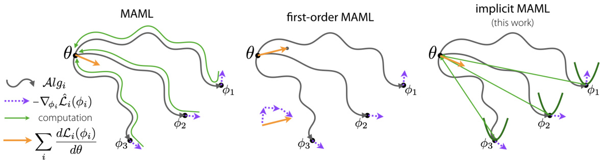
Figure 1: To compute the meta-gradient $\sum_{i}\frac{d\mathcal{L}_ {i}(\phi_{i})}{d\theta}$ , the MAML algorithm differentiates through the optimization path, as shown in green , while first-order MAML computes the meta-gradient by approximating $\frac{d\phi_{i}}{d\theta_{\ast}}$ as $\pmb{I}$ . Our implicit MAML approach derives an analytic expression for the exact meta-gradient without differentiating through the optimization path by estimating local curvature.
图 1: 为计算元梯度 $\sum_{i}\frac{d\mathcal{L}_ {i}(\phi_{i})}{d\theta}$,MAML算法通过优化路径进行微分(如绿色部分所示),而一阶MAML通过将 $\frac{d\phi_{i}}{d\theta_{\ast}}$ 近似为 $\pmb{I}$ 来计算元梯度。我们的隐式MAML方法通过估计局部曲率,在不经过优化路径微分的情况下推导出精确元梯度的解析表达式。
The main contribution of our work is the development of the implicit MAML (iMAML) algorithm, an approach for optimization-based meta-learning with deep neural networks that removes the need for differentiating through the optimization path. Our algorithm aims to learn a set of parameters such that an optimization algorithm that is initialized at and regularized to this parameter vector leads to good generalization for a variety of learning tasks. By leveraging the implicit differentiation approach, we derive an analytical expression for the meta (or outer level) gradient that depends only on the solution to the inner optimization and not the path taken by the inner optimization algorithm, as depicted in Figure 1. This decoupling of meta-gradient computation and choice of inner level optimizer has a number of appealing properties.
我们工作的主要贡献是开发了隐式MAML (iMAML) 算法,这是一种基于优化的元学习方法,适用于深度神经网络,无需对优化路径进行微分。该算法旨在学习一组参数,使得以该参数向量为初始点并对其进行正则化的优化算法能够在多种学习任务上实现良好的泛化性能。通过利用隐式微分方法,我们推导出了元梯度(或称外层梯度)的解析表达式,该表达式仅依赖于内部优化的解,而不依赖于内部优化算法所采取的路径,如图1所示。这种元梯度计算与内部优化器选择的解耦具有诸多优势。
First, the inner optimization path need not be stored nor differentiated through, thereby making implicit MAML memory efficient and scalable to a large number of inner optimization steps. Second, implicit MAML is agnostic to the inner optimization method used, as long as it can find an approximate solution to the inner-level optimization problem. This permits the use of higher-order methods, and in principle even non-differentiable optimization methods or components like samplebased optimization, line-search, or those provided by proprietary software (e.g. Gurobi). Finally, we also provide the first (to our knowledge) non-asymptotic theoretical analysis of bi-level optimization. We show that an $\epsilon\mathrm{\Omega}$ –approximate meta-gradient can be computed via implicit MAML using ${\tilde{O}}(\log(1/\epsilon))$ gradient evaluations and $\tilde{O}(1)$ memory, meaning the memory required does not grow with number of gradient steps.
首先,内层优化路径无需存储或进行微分处理,这使得隐式MAML具有内存高效性,并能扩展到大量内层优化步骤。其次,隐式MAML对所使用的内层优化方法无特定要求,只要该方法能找到内层优化问题的近似解即可。这允许使用高阶方法,甚至原则上可采用不可微优化方法或基于采样的优化、线搜索等组件,或专有软件(如Gurobi)提供的方法。最后,我们还首次(据我们所知)对双层优化进行了非渐进理论分析。研究表明,通过隐式MAML计算$\epsilon\mathrm{\Omega}$近似元梯度仅需${\tilde{O}}(\log(1/\epsilon))$次梯度评估和$\tilde{O}(1)$内存,这意味着所需内存不会随梯度步数增加而增长。
2 Problem Formulation and Notations
2 问题表述与符号说明
We first present the meta-learning problem in the context of few-shot supervised learning, and then generalize the notation to aid the rest of the exposition in the paper.
我们首先在少样本监督学习的背景下提出元学习问题,然后推广符号表示以方便论文后续阐述。
2.1 Review of Few-Shot Supervised Learning and MAML
2.1 少样本监督学习和MAML综述
In this setting, we have a collection of meta-training tasks ${\mathcal{T}_ {i}}_ {i=1}^{M}$ drawn from $P(\tau)$ . Each task $\tau_{i}$ is associated with a dataset $\mathcal{D}_ {i}$ , from which we can sample two disjoint sets: $\mathcal{D}_ {i}^{\mathrm{tr}}$ and $\mathcal{D}_ {i}^{\mathrm{test}}$ . These datasets each consist of $K$ input-output pairs. Let $\mathbf x\in\mathcal X$ and $\mathbf y\in\mathcal y$ denote inputs and outputs, respectively. The datasets take the form $\mathbf{\mathcal{D}}_ {i}^{\mathrm{tr}}={(\mathbf{x}_ {i}^{k},\mathbf{y}_ {i}^{k})}_ {k=1}^{K}$ , and similarly for $\mathcal{D}_ {i}^{\mathrm{test}}$ . We are interested in learning models of the form $h_{\phi}(\mathbf{x}):\mathcal{X}\to\mathcal{Y}$ , parameterized by $\phi\in\Phi\equiv\mathbb{R}^{d}$ . Performance on a task is specified by a loss function, such as the cross entropy or squared error loss. We will write the loss function in the form $\mathcal{L}(\phi,\mathcal{D})$ , as a function of a parameter vector and dataset. The goal for task $\tau_{i}$ is to learn task-specific parameters $\phi_{i}$ using $\mathcal{D}_ {i}^{\mathrm{tr}}$ such that we can minimize the population or test loss of the task, $\mathcal{L}(\phi_{i},\mathcal{D}_{i}^{\mathrm{test}})$ .
在此设定中,我们有一组从$P(\tau)$中抽取的元训练任务${\mathcal{T}_ {i}}_ {i=1}^{M}$。每个任务$\tau_{i}$关联一个数据集$\mathcal{D}_ {i}$,从中可采样出两个不相交的子集:$\mathcal{D}_ {i}^{\mathrm{tr}}$和$\mathcal{D}_ {i}^{\mathrm{test}}$。这些数据集各自包含$K$个输入-输出对,其中$\mathbf x\in\mathcal X$表示输入,$\mathbf y\in\mathcal y$表示输出。数据集形式为$\mathbf{\mathcal{D}}_ {i}^{\mathrm{tr}}={(\mathbf{x}_ {i}^{k},\mathbf{y}_ {i}^{k})}_ {k=1}^{K}$,$\mathcal{D}_ {i}^{\mathrm{test}}$同理。我们关注学习形式为$h_{\phi}(\mathbf{x}):\mathcal{X}\to\mathcal{Y}$的模型,其参数为$\phi\in\Phi\equiv\mathbb{R}^{d}$。任务性能由损失函数(如交叉熵或平方误差损失)衡量,记作$\mathcal{L}(\phi,\mathcal{D})$,该函数以参数向量和数据集为自变量。对于任务$\tau_{i}$,目标是通过$\mathcal{D}_ {i}^{\mathrm{tr}}$学习任务特定参数$\phi_{i}$,以最小化该任务的总体或测试损失$\mathcal{L}(\phi_{i},\mathcal{D}_{i}^{\mathrm{test}})$。
In the general bi-level meta-learning setup, we consider a space of algorithms that compute taskspecific parameters using a set of meta-parameters $\pmb{\theta}\in\Theta\overset{\pm}{=}\mathbb{R}^{d}$ and the training dataset from the task, such that $\phi_{i}=\mathcal{A}g(\pmb{\theta},\mathcal{D}_ {i}^{\mathrm{tr}})$ for task $\tau_{i}$ . The goal of meta-learning is to learn meta-parameters that produce good task specific parameters after adaptation, as specified below:
在通用的双层元学习设置中,我们考虑一个算法空间,该空间使用一组元参数 $\pmb{\theta}\in\Theta\overset{\pm}{=}\mathbb{R}^{d}$ 和任务训练数据集来计算任务特定参数,使得任务 $\tau_{i}$ 的 $\phi_{i}=\mathcal{A}g(\pmb{\theta},\mathcal{D}_{i}^{\mathrm{tr}})$。元学习的目标是学习能够在下文所述的适应后产生良好任务特定参数的元参数:
$$
\overbrace{\theta_{\mathrm{ML}}^{*}:=\underset{\theta\in\Theta}{\operatorname{argmin}}F(\theta)}^{\mathrm{outer-level}},\mathrm{where}F(\theta)=\frac{1}{M}\sum_{i=1}^{M}\mathcal{L}\left(\overbrace{\mathcal{A}l g\big(\theta,\mathcal{D}_ {i}^{\mathrm{tr}}\big)}^{\mathrm{inner-level}},\mathcal{D}_{i}^{\mathrm{test}}\right).
$$
$$
\overbrace{\theta_{\mathrm{ML}}^{*}:=\underset{\theta\in\Theta}{\operatorname{argmin}}F(\theta)}^{\mathrm{outer-level}},\mathrm{where}F(\theta)=\frac{1}{M}\sum_{i=1}^{M}\mathcal{L}\left(\overbrace{\mathcal{A}l g\big(\theta,\mathcal{D}_ {i}^{\mathrm{tr}}\big)}^{\mathrm{inner-level}},\mathcal{D}_{i}^{\mathrm{test}}\right).
$$
We view this as a bi-level optimization problem since we typically interpret $\mathcal{A}l g\big(\pmb{\theta},\mathcal{D}_ {i}^{\mathrm{tr}}\big)$ as either explicitly or implicitly solving an underlying optimization problem. At meta-test (deployment) time, when presented with a dataset $\mathcal{D}_ {j}^{\mathrm{tr}}$ corresponding to a new task $\tau_{j}\sim P(\tau)$ , we can achieve good generalization performance (i.e., low test error) by using the adaptation procedure with the metalearned parameters as $\phi_{j}=\mathcal{A}l g(\theta_{\mathrm{ML}}^{*},\mathcal{D}_{j}^{\mathrm{tr}})$ .
我们将此视为一个双层优化问题,因为通常将$\mathcal{A}l g\big(\pmb{\theta},\mathcal{D}_ {i}^{\mathrm{tr}}\big)$解释为显式或隐式地解决一个底层优化问题。在元测试(部署)阶段,当遇到对应于新任务$\tau_ {j}\sim P(\tau)$的数据集$\mathcal{D}_ {j}^{\mathrm{tr}}$时,通过使用以元学习参数$\phi_{j}=\mathcal{A}l g(\theta_{\mathrm{ML}}^{*},\mathcal{D}_{j}^{\mathrm{tr}})$的适应过程,可以获得良好的泛化性能(即低测试误差)。
In the case of MAML [15], ${\mathcal{A l g}}(\theta,{\mathcal{D}})$ corresponds to one or multiple steps of gradient descent initialized at $\pmb{\theta}$ . For example, if one step of gradient descent is used, we have:
在MAML [15]的情况下,${\mathcal{A l g}}(\theta,{\mathcal{D}})$对应于在$\pmb{\theta}$初始化时进行的一步或多步梯度下降。例如,如果使用一步梯度下降,则有:
$$
\phi_{i}\equiv A l g(\pmb{\theta},\mathcal{D}_ {i}^{\mathrm{tr}})=\pmb{\theta}-\alpha\nabla_{\pmb{\theta}}\mathcal{L}(\pmb{\theta},\mathcal{D}_{i}^{\mathrm{tr}}).
$$
$$
\phi_{i}\equiv A l g(\pmb{\theta},\mathcal{D}_ {i}^{\mathrm{tr}})=\pmb{\theta}-\alpha\nabla_{\pmb{\theta}}\mathcal{L}(\pmb{\theta},\mathcal{D}_{i}^{\mathrm{tr}}).
$$
Typically, $\alpha$ is a scalar hyper parameter, but can also be a learned vector [34]. Hence, for MAML, the meta-learned parameter $(\pmb{\theta}_{\mathrm{ML}}^{*})$ has a learned inductive bias that is particularly well-suited for finetuning on tasks from $P(\tau)$ using $K$ samples. To solve the outer-level problem with gradient-based methods, we require a way to differentiate through $\boldsymbol{\mathcal{A}}\boldsymbol{l}\boldsymbol{g}$ . In the case of MAML, this corresponds to back propagating through the dynamics of gradient descent.
通常,$\alpha$ 是一个标量超参数,但也可以是一个可学习的向量 [34]。因此,对于 MAML 来说,元学习参数 $(\pmb{\theta}_{\mathrm{ML}}^{*})$ 具有一种特别适合在 $P(\tau)$ 上使用 $K$ 个样本进行微调的学习归纳偏置。为了用基于梯度的方法解决外层问题,我们需要一种方法来对 $\boldsymbol{\mathcal{A}}\boldsymbol{l}\boldsymbol{g}$ 进行微分。在 MAML 的情况下,这对应于通过梯度下降的动态进行反向传播。
2.2 Proximal Regular iz ation in the Inner Level
2.2 内层近端正则化
To have sufficient learning in the inner level while also avoiding over-fitting, $\boldsymbol{\mathcal{A}}l\boldsymbol{g}$ needs to incorporate some form of regular iz ation. Since MAML uses a small number of gradient steps, this corresponds to early stopping and can be interpreted as a form of regular iz ation and Bayesian prior [20]. In cases like ill-conditioned optimization landscapes and medium-shot learning, we may want to take many gradient steps, which poses two challenges for MAML. First, we need to store and differentiate through the long optimization path of $\boldsymbol{\mathcal{A}}l\boldsymbol{g}$ , which imposes a considerable computation and memory burden. Second, the dependence of the model-parameters ${\phi_{i}}$ on the meta-parameters $(\pmb\theta)$ shrinks and vanishes as the number of gradient steps in $\boldsymbol{\mathcal{A}}\boldsymbol{l}\boldsymbol{g}$ grows, making meta-learning difficult. To overcome these limitations, we consider a more explicitly regularized algorithm:
为了在内部层级实现充分学习的同时避免过拟合,$\boldsymbol{\mathcal{A}}l\boldsymbol{g}$需要引入某种形式的正则化。由于MAML采用少量梯度步长,这相当于早停机制,可视为一种正则化形式及贝叶斯先验[20]。在病态优化场景和中样本学习等情况下,我们可能需要进行大量梯度步骤,这为MAML带来两个挑战:首先需要存储并区分$\boldsymbol{\mathcal{A}}l\boldsymbol{g}$的长优化路径,这会带来巨大的计算和内存负担;其次随着$\boldsymbol{\mathcal{A}}\boldsymbol{l}\boldsymbol{g}$中梯度步数的增加,模型参数${\phi_{i}}$对元参数$(\pmb\theta)$的依赖会逐渐缩小直至消失,导致元学习困难。为突破这些限制,我们考虑采用显式正则化算法:
$$
\varLambda l g^{\star}(\theta,\mathcal{D}_ {i}^{\mathrm{tr}})=\operatorname*{argmin}_ {\phi^{\prime}\in\Phi}\mathcal{L}(\phi^{\prime},\mathcal{D}_{i}^{\mathrm{tr}})+\frac{\lambda}{2}||\phi^{\prime}-\theta||^{2}.
$$
$$
\varLambda l g^{\star}(\theta,\mathcal{D}_ {i}^{\mathrm{tr}})=\operatorname*{argmin}_ {\phi^{\prime}\in\Phi}\mathcal{L}(\phi^{\prime},\mathcal{D}_{i}^{\mathrm{tr}})+\frac{\lambda}{2}||\phi^{\prime}-\theta||^{2}.
$$
The proximal regular iz ation term in Eq. 3 encourages $\phi_{i}$ to remain close to $\pmb{\theta}$ , thereby retaining a strong dependence throughout. The regular iz ation strength $(\lambda)$ plays a role similar to the learning rate $(\alpha)$ in MAML, controlling the strength of the prior $(\pmb\theta)$ relative to the data $\left(\mathcal{D}_{\mathcal{T}}^{\mathrm{tr}}\right)$ . Like $\alpha$ , the regular iz ation strength $\lambda$ may also be learned. Furthermore, both $\alpha$ and $\lambda$ can be scalars, vectors, or full matrices. For simplicity, we treat $\lambda$ as a scalar hyper parameter. In Eq. 3, we use $\star$ to denote that the optimization problem is solved exactly. In practice, we use iterative algorithms (denoted by ${\mathcal{A}}l g)$ ) for finite iterations, which return approximate minimizers. We explicitly consider the discrepancy between approximate and exact solutions in our analysis.
式3中的近端正则化项促使$\phi_{i}$保持接近$\pmb{\theta}$,从而始终保持强依赖性。正则化强度$(\lambda)$的作用类似于MAML中的学习率$(\alpha)$,控制先验$(\pmb\theta)$相对于数据$\left(\mathcal{D}_{\mathcal{T}}^{\mathrm{tr}}\right)$的强度。与$\alpha$类似,正则化强度$\lambda$也可以学习。此外,$\alpha$和$\lambda$都可以是标量、向量或完整矩阵。为简单起见,我们将$\lambda$视为标量超参数。在式3中,使用$\star$表示优化问题被精确求解。实际中,我们使用迭代算法(记为${\mathcal{A}}l g)$)进行有限次迭代,返回近似最小值。在分析中我们明确考虑了近似解与精确解之间的差异。
2.3 The Bi-Level Optimization Problem
2.3 双层优化问题
For notation convenience, we will sometimes express the dependence on task $\tau_{i}$ using a subscript instead of arguments, e.g. we write:
为方便标记,我们有时会用下标而非参数表示对任务$\tau_{i}$的依赖关系,例如写作:
$$
\mathcal{L}_ {i}(\boldsymbol{\phi}):=\mathcal{L}\big(\boldsymbol{\phi},\mathcal{D}_ {i}^{\mathrm{test}}\big),\quad\hat{\mathcal{L}}_ {i}(\boldsymbol{\phi}):=\mathcal{L}\big(\boldsymbol{\phi},\mathcal{D}_ {i}^{\mathrm{tr}}\big),\quad\mathcal{A}l g_{i}(\boldsymbol{\theta}):=\mathcal{A}l g\big(\boldsymbol{\theta},\mathcal{D}_{i}^{\mathrm{tr}}\big).
$$
$$
\mathcal{L}_ {i}(\boldsymbol{\phi}):=\mathcal{L}\big(\boldsymbol{\phi},\mathcal{D}_ {i}^{\mathrm{test}}\big),\quad\hat{\mathcal{L}}_ {i}(\boldsymbol{\phi}):=\mathcal{L}\big(\boldsymbol{\phi},\mathcal{D}_ {i}^{\mathrm{tr}}\big),\quad\mathcal{A}l g_{i}(\boldsymbol{\theta}):=\mathcal{A}l g\big(\boldsymbol{\theta},\mathcal{D}_{i}^{\mathrm{tr}}\big).
$$
With this notation, the bi-level meta-learning problem can be written more generally as:
采用这种表示法,双层元学习问题可以更一般地表示为:
$$
\begin{array}{r l}&{\theta_{\mathrm{ML}}^{*}:=\underset{\theta\in\Theta}{\operatorname{argmin}}F(\theta)\mathrm{,where~}F(\theta)=\frac{1}{M}\displaystyle\sum_{i=1}^{M}\mathcal{L}_ {i}\big(\mathcal{A}l g_{i}^{\star}(\theta)\big),\mathrm{and}}\ &{\mathcal{A}l g_{i}^{\star}(\theta):=\underset{\phi^{\prime}\in\Phi}{\operatorname{argmin}}G_{i}(\phi^{\prime},\theta)\mathrm{,where~}G_{i}(\phi^{\prime},\theta)=\hat{\mathcal{L}}_{i}(\phi^{\prime})+\frac{\lambda}{2}||\phi^{\prime}-\theta||^{2}\mathrm{.}}\end{array}
$$
$$
\begin{array}{r l}&{\theta_{\mathrm{ML}}^{*}:=\underset{\theta\in\Theta}{\operatorname{argmin}}F(\theta)\mathrm{,其中~}F(\theta)=\frac{1}{M}\displaystyle\sum_{i=1}^{M}\mathcal{L}_ {i}\big(\mathcal{A}l g_{i}^{\star}(\theta)\big)\mathrm{,~且}}\ &{\mathcal{A}l g_{i}^{\star}(\theta):=\underset{\phi^{\prime}\in\Phi}{\operatorname{argmin}}G_{i}(\phi^{\prime},\theta)\mathrm{,其中}G_{i}(\phi^{\prime},\theta)=\hat{\mathcal{L}}_{i}(\phi^{\prime})+\frac{\lambda}{2}||\phi^{\prime}-\theta||^{2}\mathrm{.}}\end{array}
$$
2.4 Total and Partial Derivatives
2.4 全微分与偏微分
We use $^d$ to denote the total derivative and $\nabla$ to denote partial derivative. For nested function of the form $\mathcal{L}_ {i}(\phi_{i})$ where $\phi_{i}=\mathcal{A}l g_{i}(\pmb{\theta})$ , we have from chain rule
我们用 $^d$ 表示全导数,用 $\nabla$ 表示偏导数。对于形如 $\mathcal{L}_ {i}(\phi_{i})$ 的嵌套函数,其中 $\phi_{i}=\mathcal{A}l g_{i}(\pmb{\theta})$ ,根据链式法则可得
$$
d_{\theta}\mathcal{L}_ {i}(\mathcal{A}l g_{i}(\theta))=\frac{d\mathcal{A}l g_{i}(\theta)}{d\theta}\nabla_{\phi}\mathcal{L}_ {i}(\phi)\mid_{\phi=\mathcal{A}l g_{i}(\theta)}=\frac{d\mathcal{A}l g_{i}(\theta)}{d\theta}\nabla_{\phi}\mathcal{L}_{i}(\mathcal{A}l g_ {i}(\theta))
$$
$$
d_{\theta}\mathcal{L}_ {i}(\mathcal{A}l g_{i}(\theta))=\frac{d\mathcal{A}l g_{i}(\theta)}{d\theta}\nabla_{\phi}\mathcal{L}_ {i}(\phi)\mid_{\phi=\mathcal{A}l g_{i}(\theta)}=\frac{d\mathcal{A}l g_{i}(\theta)}{d\theta}\nabla_{\phi}\mathcal{L}_ {i}(\mathcal{A}l g_{i}(\theta))
$$
Note the important distinction between $d_{\theta}\mathscr{L}_ {i}(\mathcal{A}g_{i}(\pmb{\theta}))$ and $\nabla_{\phi}\mathcal{L}_ {i}(\mathcal{A}l g_{i}(\pmb{\theta}))$ . The former passes derivatives through $\boldsymbol{\mathcal{A}}l g_{i}(\pmb{\theta})$ while the latter does not. $\nabla_{\phi}\mathcal{L}_ {i}(\mathcal{A}\dot{l}g_{i}(\pmb{\theta}))$ is simply the gradient function, i.e. $\nabla_{\phi}\mathcal{L}_ {i}(\phi)$ , evaluated at $\phi=\mathcal{A}g_{i}(\pmb\theta)$ . Also note that $d_{\theta}\mathcal{L}_ {i}(\mathcal{A}g_{i}(\pmb{\theta}))$ and $\bar{\nabla_{\pmb{\phi}}}\mathcal{L}_ {i}(\mathcal{A}l g_{i}(\pmb{\theta}))$ are d–dimensional vectors, while dAldgθi(θ) i s a $(d\times d)$ –size Jacobian matrix. Throughout this text, we will also use $d_{\theta}$ and $\frac{d}{d\theta}$ interchangeably.
注意区分 $d_{\theta}\mathscr{L}_ {i}(\mathcal{A}g_{i}(\pmb{\theta}))$ 和 $\nabla_{\phi}\mathcal{L}_ {i}(\mathcal{A}l g_{i}(\pmb{\theta}))$ 的重要区别。前者通过 $\boldsymbol{\mathcal{A}}l g_{i}(\pmb{\theta})$ 传递导数,而后者则不会。$\nabla_{\phi}\mathcal{L}_ {i}(\mathcal{A}\dot{l}g_{i}(\pmb{\theta}))$ 只是梯度函数,即在 $\phi=\mathcal{A}g_{i}(\pmb\theta)$ 处评估的 $\nabla_{\phi}\mathcal{L}_ {i}(\phi)$。还需注意 $d_{\theta}\mathcal{L}_ {i}(\mathcal{A}g_{i}(\pmb{\theta}))$ 和 $\bar{\nabla_{\pmb{\phi}}}\mathcal{L}_ {i}(\mathcal{A}l g_{i}(\pmb{\theta}))$ 是 d 维向量,而 dAldgθi(θ) 是一个 $(d\times d)$ 大小的雅可比矩阵。在本文中,我们将交替使用 $d_{\theta}$ 和 $\frac{d}{d\theta}$。
3 The Implicit MAML Algorithm
3 隐式 MAML 算法
Our aim is to solve the bi-level meta-learning problem in Eq. 4 using an iterative gradient based algorithm of the form $\theta\leftarrow\theta-\eta d_{\theta}F(\theta)$ . Although we derive our method based on standard gradient descent for simplicity, any other optimization method, such as quasi-Newton or Newton methods, Adam [28], or gradient descent with momentum can also be used without modification. The gradient descent update be expanded using the chain rule as
我们的目标是通过基于梯度的迭代算法求解公式4中的双层元学习问题,其形式为$\theta\leftarrow\theta-\eta d_{\theta}F(\theta)$。虽然为简化推导我们采用标准梯度下降法,但该方法同样适用于其他优化算法(如拟牛顿法、牛顿法、Adam [28] 或带动量的梯度下降)且无需修改。根据链式法则,梯度下降更新可展开为
$$
\theta\leftarrow\theta-\eta\frac{1}{M}\sum_{i=1}^{M}\frac{d\boldsymbol{A}l g_{i}^{\star}(\theta)}{d\theta}\nabla_{\phi}\mathcal{L}_ {i}(\boldsymbol{A}l g_{i}^{\star}(\theta)).
$$
$$
\theta\leftarrow\theta-\eta\frac{1}{M}\sum_{i=1}^{M}\frac{d\boldsymbol{A}l g_{i}^{\star}(\theta)}{d\theta}\nabla_{\phi}\mathcal{L}_ {i}(\boldsymbol{A}l g_{i}^{\star}(\theta)).
$$
Here, $\nabla_{\phi}\mathcal{L}_ {i}(\mathcal{A}l g_{i}^{\star}(\pmb{\theta}))$ is simply $\nabla_{\phi}\mathcal{L}_ {i}(\phi)\mid_{\phi=\mathcal{A}l g_{i}^{\star}(\pmb\theta)}$ which can be easily obtained in practice via automatic differentiation. For this update rule, we must compute dAldgθi (θ) , where Algi⋆ is implicitly defined as an optimization problem (Eq. 4), which presents the primary challenge. We now present an efficient algorithm (in compute and memory) to compute the meta-gradient..
这里,$\nabla_{\phi}\mathcal{L}_ {i}(\mathcal{A}l g_{i}^{\star}(\pmb{\theta}))$ 其实就是 $\nabla_{\phi}\mathcal{L}_ {i}(\phi)\mid_{\phi=\mathcal{A}l g_{i}^{\star}(\pmb\theta)}$,实践中可通过自动微分轻松获得。对于该更新规则,我们必须计算 dAldgθi (θ),其中 Algi⋆ 被隐式定义为优化问题(式4),这是主要挑战所在。现在我们提出一种高效算法(计算和内存方面)来计算元梯度。
3.1 Meta-Gradient Computation
3.1 元梯度计算
If $\mathcal{A}l g_{i}^{\star}(\pmb\theta)$ is implemented as an iterative algorithm, such as gradient descent, then one way to compute dAldgθi⋆ (θ) is to propagate derivatives through the iterative process, either in forward mode or reverse mode. However, this has the drawback of depending explicitly on the path of the optimization, which has to be fully stored in memory, quickly becoming intractable when the number of gradient steps needed is large. Furthermore, for second order optimization methods, such as Newton’s method, third derivatives are needed which are difficult to obtain. Furthermore, this approach becomes impossible when non-differentiable operations, such as line-searches, are used. However, by recognizing that $\boldsymbol{\mathcal{A}}\boldsymbol{l}g_{i}^{\star}$ is implicitly defined as the solution to an optimization problem, we may employ a different strategy that does not need to consider the path of the optimization but only the final result. This is derived in the following Lemma.
如果 $\mathcal{A}l g_{i}^{\star}(\pmb\theta)$ 是通过迭代算法(如梯度下降)实现的,那么计算 dAldgθi⋆ (θ) 的一种方式是通过前向模式或反向模式在迭代过程中传播导数。然而,这种方法存在明显依赖于优化路径的缺点,需要完整存储路径信息,当所需梯度步数较多时会迅速变得难以处理。此外,对于牛顿法等二阶优化方法,需要难以获取的三阶导数。更关键的是,当采用不可微分操作(如线性搜索)时,这种方法将完全失效。但通过认识到 $\boldsymbol{\mathcal{A}}\boldsymbol{l}g_{i}^{\star}$ 是作为优化问题的解被隐式定义的,我们可以采用不同策略——该策略只需考虑优化结果而无需追踪优化路径。具体推导见下述引理。
Lemma 1. (Implicit Jacobian) Consider $\mathcal{A}l g_{i}^{\star}(\pmb\theta)$ as defined in Eq. 4 for task $\tau_{i}$ . Let $\phi_{i}=\mathcal{A}g_{i}^{\star}(\pmb\theta)$ be the result of $\mathcal{A}l g_{i}^{\star}(\pmb\theta)$ . If $\begin{array}{r}{\left(I+\frac{1}{\lambda}\nabla_{\phi}^{2}\hat{\mathcal{L}}_ {i}(\phi_{i})\right)}\end{array}$ is invertible, then the derivative Jacobian is
引理 1. (隐式雅可比矩阵) 考虑任务 $\tau_{i}$ 中由式4定义的 $\mathcal{A}l g_{i}^{\star}(\pmb\theta)$ 。设 $\phi_{i}=\mathcal{A}g_{i}^{\star}(\pmb\theta)$ 为 $\mathcal{A}l g_{i}^{\star}(\pmb\theta)$ 的结果。若 $\begin{array}{r}{\left(I+\frac{1}{\lambda}\nabla_{\phi}^{2}\hat{\mathcal{L}}_ {i}(\phi_{i})\right)}\end{array}$ 可逆,则导数雅可比矩阵为
$$
\frac{d\mathcal{A}l g_{i}^{\star}(\pmb\theta)}{d\pmb\theta}=\left(\pmb I+\frac{1}{\lambda}\nabla_{\phi}^{2}\hat{\mathcal{L}}_ {i}(\phi_{i})\right)^{-1}.
$$
$$
\frac{d\mathcal{A}l g_{i}^{\star}(\pmb\theta)}{d\pmb\theta}=\left(\pmb I+\frac{1}{\lambda}\nabla_{\phi}^{2}\hat{\mathcal{L}}_ {i}(\phi_{i})\right)^{-1}.
$$
Note that the derivative (Jacobian) depends only on the final result of the algorithm, and not the path taken by the algorithm. Thus, in principle any approach of algorithm can be used to compute $\mathcal{A}l g_{i}^{\star}(\pmb\theta)$ , thereby decoupling meta-gradient computation from choice of inner level optimizer.
请注意,导数(雅可比矩阵)仅取决于算法的最终结果,而不依赖于算法所采取的路径。因此,原则上可以使用任何算法方法来计算 $\mathcal{A}l g_{i}^{\star}(\pmb\theta)$ ,从而将元梯度计算与内层优化器的选择解耦。
Practical Algorithm: While Lemma 1 provides an idealized way to compute the $\boldsymbol{\mathcal{A}}\boldsymbol{l}g_{i}^{\star}$ Jacobians and thus by extension the meta-gradient, it may be difficult to directly use it in practice. Two issues are particularly relevant. First, the meta-gradients require computation of $\mathcal{A}l g_{i}^{\star}(\pmb\theta)$ , which is the exact solution to the inner optimization problem. In practice, we may be able to obtain only approximate solutions. Second, explicitly forming and inverting the matrix in Eq. 6 for computing the Jacobian may be intractable for large deep neural networks. To address these difficulties, we consider approximations to the idealized approach that enable a practical algorithm.
实用算法:虽然引理1提供了一种理想化的方法来计算$\boldsymbol{\mathcal{A}}\boldsymbol{l}g_{i}^{\star}$雅可比矩阵,进而计算元梯度,但在实践中直接使用可能存在困难。其中两个问题尤为突出:首先,元梯度需要计算$\mathcal{A}l g_{i}^{\star}(\pmb\theta)$,即内部优化问题的精确解,而实践中通常只能获得近似解;其次,对于大型深度神经网络,显式构建并求逆公式6中的矩阵以计算雅可比矩阵可能难以实现。为解决这些问题,我们考虑对理想化方法进行近似,从而得到实用算法。
First, we consider an approximate solution to the inner optimization problem, that can be obtained with iterative optimization algorithms like gradient descent.
首先,我们考虑内层优化问题的近似解,可通过梯度下降等迭代优化算法获得。
Definition 1. ( $\mathit{\check{\Delta}}$ –approx. algorithm) Let $\boldsymbol{\mathcal{A}}l g_{i}(\pmb{\theta})$ be a $\delta$ –accurate approximation of $\mathcal{A}l g_{i}^{\star}(\pmb\theta)$ , i.e.
定义1. ( $\mathit{\check{\Delta}}$ –近似算法) 设 $\boldsymbol{\mathcal{A}}l g_{i}(\pmb{\theta})$ 是 $\mathcal{A}l g_{i}^{\star}(\pmb\theta)$ 的 $\delta$ –精确近似,即
$$
\lVert\mathcal{A}l g_{i}({\pmb\theta})-\mathcal{A}l g_{i}^{\star}({\pmb\theta})\rVert\le\delta
$$
$$
\lVert\mathcal{A}l g_{i}({\pmb\theta})-\mathcal{A}l g_{i}^{\star}({\pmb\theta})\rVert\le\delta
$$
Algorithm 2 Implicit Meta-Gradient Computation
算法 2: 隐式元梯度计算
Second, we will perform a partial or approximate matrix inversion given by:
其次,我们将执行由下式给出的部分或近似矩阵求逆:
Definition 2. ( $'\delta^{\prime}$ –approximate Jacobian-vector product) Let ${\mathbf{}}_ {}{\mathbf{}}_ {3}{\mathbf{}}_{i}$ be a vector such tha
定义 2. ( $'\delta^{\prime}$ –近似雅可比向量积) 设 ${\mathbf{}}_ {}{\mathbf{}}_ {3}{\mathbf{}}_{i}$ 为满足以下条件的向量
$$
|g_{i}-\left(I+\frac{1}{\lambda}\nabla_{\phi}^{2}\hat{\mathcal{L}}_ {i}(\phi_{i})\right)^{-1}\nabla_{\phi}\mathcal{L}_ {i}(\phi_{i})|\leq\delta^{\prime}
$$
$$
|g_{i}-\left(I+\frac{1}{\lambda}\nabla_{\phi}^{2}\hat{\mathcal{L}}_ {i}(\phi_{i})\right)^{-1}\nabla_{\phi}\mathcal{L}_ {i}(\phi_{i})|\leq\delta^{\prime}
$$
where $\phi_{i}=\mathcal{A}g_{i}(\pmb\theta)$ and $\boldsymbol{\mathcal{A}}\boldsymbol{l}_ {\boldsymbol{\mathit{g}}_{i}}$ is based on definition $I$ .
其中 $\phi_{i}=\mathcal{A}g_{i}(\pmb\theta)$,且 $\boldsymbol{\mathcal{A}}\boldsymbol{l}_ {\boldsymbol{\mathit{g}}_{i}}$ 基于定义 $I$。
Note that ${\mathbf{}}_ {}{\mathbf{}}_ {3}{\mathbf{}}_ {i}$ in definition 2 is an approximation of the meta-gradient for task $\tau_{i}$ . Observe that ${\mathbf{}}_ {}{\mathbf{}}_ {3}{\mathbf{}}_{i}$ can be obtained as an approximate solution to the optimization problem:
注意,定义2中的 ${\mathbf{}}_ {}{\mathbf{}}_ {3}{\mathbf{}}_ {i}$ 是任务 $\tau_{i}$ 元梯度的近似值。可以看出 ${\mathbf{}}_ {}{\mathbf{}}_ {3}{\mathbf{}}_{i}$ 可作为以下优化问题的近似解:
$$
\operatorname*{min}_ {\pmb{w}}\pmb{w}^{\top}\bigg(\pmb{I}+\frac{1}{\lambda}~\nabla_{\phi}^{2}\hat{\mathcal{L}}_ {i}(\phi_{i})\bigg)\pmb{w}-\pmb{w}^{\top}\nabla_{\phi}\mathcal{L}_ {i}(\phi_{i})
$$
$$
\operatorname*{min}_ {\pmb{w}}\pmb{w}^{\top}\bigg(\pmb{I}+\frac{1}{\lambda}~\nabla_{\phi}^{2}\hat{\mathcal{L}}_ {i}(\phi_{i})\bigg)\pmb{w}-\pmb{w}^{\top}\nabla_{\phi}\mathcal{L}_ {i}(\phi_{i})
$$
The conjugate gradient (CG) algorithm is particularly well suited for this problem due to its excellent iteration complexity and requirement of only Hessian-vector products of the form $\nabla^{2}\hat{\mathcal{L}}_ {i}(\phi_{i})\pmb{v}$ . Such hessian-vector products can be obtained cheaply without explicitly forming or storing the Hessian matrix (as we discuss in Appendix C). This CG based inversion has been successfully deployed in Hessian-free or Newton-CG methods for deep learning [36, 44] and trust region methods in rein for cement learning [52, 47]. Algorithm 1 presents the full practical algorithm. Note that these approximations to develop a practical algorithm introduce errors in the meta-gradient computation. We analyze the impact of these errors in Section 3.2 and show that they are controllable. See Appendix A for how iMAML generalizes prior gradient optimization based meta-learning algorithms.
共轭梯度 (CG) 算法因其优异的迭代复杂度和仅需计算形式为 $\nabla^{2}\hat{\mathcal{L}}_ {i}(\phi_{i})\pmb{v}$ 的海森矩阵-向量积的特性,特别适合解决该问题。此类海森矩阵-向量积无需显式构建或存储海森矩阵即可高效计算(如附录C所述)。这种基于CG的求逆方法已成功应用于深度学习的无海森矩阵方法或牛顿-CG方法 [36, 44] 以及强化学习中的信任域方法 [52, 47]。算法1展示了完整的实用算法。需注意,这些用于构建实用算法的近似处理会引入元梯度计算误差。我们将在3.2节分析这些误差的影响,并证明其可控性。关于iMAML如何泛化基于梯度优化的元学习算法,详见附录A。
3.2 Theory
3.2 理论
In Section 3.1, we outlined a practical algorithm that makes approximations to the idealized update rule of Eq. 5. Here, we attempt to analyze the impact of these approximations, and also understand the computation and memory requirements of iMAML. We find that iMAML can match the minimax computational complexity of back propagating through the path of the inner optimizer, but is substantially better in terms of memory usage. This work to our knowledge also provides the first non-asymptotic result that analyzes approximation error due to implicit gradients. Theorem 1 provides the computational and memory complexity for obtaining an $\epsilon\cdot$ –approximate meta-gradient. We assume $\mathcal{L}_ {i}$ is smooth but do not require it to be convex. We assume that $G_{i}$ in Eq. 4 is strongly convex, which can be made possible by appropriate choice of $\lambda$ . The key to our analysis is a second order Lipshitz assumption, i.e. $\hat{\mathcal{L}}_{i}(\cdot)$ is $\rho$ -Lipshitz Hessian. This assumption and setting has received considerable attention in recent optimization and deep learning literature [26, 42].
在第3.1节中,我们概述了一种对公式5的理想化更新规则进行近似的实用算法。在此,我们试图分析这些近似的影响,并理解iMAML的计算和内存需求。我们发现iMAML可以达到与反向传播内层优化路径相同的极小极大计算复杂度,但在内存使用方面明显更优。据我们所知,这项工作还首次提供了分析隐式梯度导致近似误差的非渐进性结果。定理1给出了获得$\epsilon\cdot$近似元梯度的计算和内存复杂度。我们假设$\mathcal{L}_ {i}$是平滑的,但不要求它是凸的。假设公式4中的$G_{i}$是强凸的,这可以通过适当选择$\lambda$来实现。我们分析的关键在于二阶Lipschitz假设,即$\hat{\mathcal{L}}_{i}(\cdot)$具有$\rho$-Lipschitz Hessian。这一假设和设定在最近的优化和深度学习文献中受到了广泛关注[26, 42]。
Table 1: Compute and memory for computing the meta-gradient when using a $\delta\cdot$ –accurate $\boldsymbol{\mathcal{A}}\boldsymbol{l}\boldsymbol{g}_ {i}$ , and the corresponding approximation error. Our compute time is measured in terms of the number of $\nabla\hat{\mathcal{L}}_ {i}$ computations. All results are in $\tilde{O}(\cdot)$ notation, which hide additional log factors; the error bound hides additional problem dependent Lipshitz and smoothness parameters (see the respective Theorem statements). $\kappa\geq1$ is the condition number for inner objective $G_{i}$ (see Equation 4), and $D$ is the diameter of the search space. The notions of error are subtly different: we assume all methods solve the inner optimization to error level of $\delta$ (as per definition 1). For our algorithm, the error refers to the $\ell_{2}$ error in the computation of $d_{\theta}\mathcal{L}_ {i}(\mathcal{A}l g_{i}^{\star}(\pmb{\theta}))$ . For the other algorithms, the error refers to the $\ell_{2}$ error in the computation of $d_{\theta}\mathcal{L}_ {i}(\mathcal{A}g_{i}(\pmb{\theta}))$ . We use Prop 3.1 of Shaban et al. [53] to provide the guarantee we use. See Appendix D for additional discussion.
表1: 使用$\delta\cdot$精度$\boldsymbol{\mathcal{A}}\boldsymbol{l}\boldsymbol{g}_ {i}$计算元梯度时的计算量与内存需求及对应近似误差。我们的计算时间以$\nabla\hat{\mathcal{L}}_ {i}$的计算次数衡量。所有结果采用$\tilde{O}(\cdot)$表示法(隐藏了对数因子);误差界还隐含了问题相关的Lipschitz和平滑性参数(参见相应定理陈述)。$\kappa\geq1$表示内部目标函数$G_{i}$的条件数(见公式4),$D$为搜索空间直径。误差定义存在细微差异:我们假设所有方法都将内部优化求解至$\delta$误差水平(根据定义1)。对本算法,误差指$d_{\theta}\mathcal{L}_ {i}(\mathcal{A}l g_{i}^{\star}(\pmb{\theta}))$计算的$\ell_{2}$误差;其他算法则指$d_{\theta}\mathcal{L}_ {i}(\mathcal{A}g_{i}(\pmb{\theta}))$计算的$\ell_{2}$误差。我们采用Shaban等[53]的命题3.1来提供所用保证。更多讨论见附录D。
| Algorithm | Compute | Memory | Error |
| MAML (GD + full back-prop) | klog() | Mem(VLi) ·k log () | 0 |
| MAML (Nesterov's AGD + full back-prop) | Vklog() | Mem(VLi) · √k log () | 0 |
| Truncated back-prop [53] (GD) | klog () | Mem(VLi) · k log () | E |
| Implicit MAML (this work) | Vklog() | Mem(VL) |
| 算法 | 计算量 | 内存占用 | 误差 |
|---|---|---|---|
| MAML (GD + 全反向传播) | klog() | Mem(VLi) ·k log () | 0 |
| MAML (Nesterov加速梯度下降 + 全反向传播) | Vklog() | Mem(VLi) · √k log () | 0 |
| 截断反向传播 [53] (梯度下降) | klog () | Mem(VLi) · k log () | E |
| 隐式MAML (本工作) | Vklog() | Mem(VL) |
Table 1 summarizes our complexity results and compares with MAML and truncated backpropagation [53] through the path of the inner optimizer. We use $\kappa$ to denote the condition number of the inner problem induced by $G_{i}$ (see Equation 4), which can be viewed as a measure of hardness of the inner optimization problem. ${\bf M e m}(\nabla\hat{\mathcal{L}}_ {i})$ is the memory taken to compute a single derivative $\nabla\hat{\mathcal{L}}_ {i}$ . Under the assumption that Hessian vector products are computed with the reverse mode of auto differentiation, we will have that both: the compute time and memory used for computing a Hessian vector product are with a (universal) constant factor of the compute time and memory used for computing $\nabla\hat{\mathcal{L}}_ {i}$ itself (see Appendix C). This allows us to measure the compute time in terms of the number of $\nabla\hat{\mathcal{L}}_{i}$ computations. We refer readers to Appendix D for additional discussion about the algorithms and their trade-offs.
表 1: 总结了我们的复杂度结果,并与通过内部优化器路径的 MAML 和截断反向传播 [53] 进行了对比。我们用 $\kappa$ 表示由 $G_{i}$ 引发的内部问题的条件数 (见公式 4),这可以视为内部优化问题难度的衡量指标。${\bf M e m}(\nabla\hat{\mathcal{L}}_ {i})$ 是计算单个导数 $\nabla\hat{\mathcal{L}}_ {i}$ 所需的内存。在假设 Hessian 向量积是通过自动微分的反向模式计算的情况下,计算 Hessian 向量积所用的时间和内存都与计算 $\nabla\hat{\mathcal{L}}_ {i}$ 本身所用的时间和内存成 (通用) 常数倍关系 (见附录 C)。这使得我们可以用 $\nabla\hat{\mathcal{L}}_{i}$ 的计算次数来衡量计算时间。关于算法及其权衡的更多讨论,请读者参阅附录 D。
Our main theorem is as follows:
我们的主要定理如下:
Theorem 1. (Informal Statement; Approximation error in Algorithm 2) Suppose that: $\mathcal{L}_ {i}(\cdot)$ is $B$ Lipshitz and $L$ smooth function; that $G_{i}(\cdot,\pmb\theta)$ (in Eq. 4) is a $\mu$ -strongly convex function with condition number $\kappa$ ; that $D$ is the diameter of search space for $\phi$ in the inner optimization problem (i.e. $|\mathcal{A}l g_{i}^{\star}(\pmb\theta)|\le D)$ ; and $\hat{\mathcal{L}}_{i}(\cdot)$ is $\rho$ -Lipshitz Hessian.
定理1. (非正式表述; 算法2的近似误差) 假设: $\mathcal{L}_ {i}(\cdot)$ 是 $B$ Lipschitz且 $L$ 光滑的函数; $G_{i}(\cdot,\pmb\theta)$ (式4中)是一个条件数为 $\kappa$ 的 $\mu$ 强凸函数; $D$ 是内层优化问题中 $\phi$ 搜索空间的直径 (即 $|\mathcal{A}l g_{i}^{\star}(\pmb\theta)|\le D)$; 且 $\hat{\mathcal{L}}_{i}(\cdot)$ 具有 $\rho$ Lipschitz Hessian。
Let ${\mathbf{}}_ {}{\mathbf{}}_ {3}{\mathbf{}}_{i}$ be the task meta-gradient returned by Algorithm 2. For any task $i$ and desired accuracy level ϵ, Algorithm 2 computes an approximate task-specific meta-gradient with the following guarantee:
设 ${\mathbf{}}_ {}{\mathbf{}}_ {3}{\mathbf{}}_{i}$ 为算法2返回的任务元梯度。对于任意任务 $i$ 和期望精度水平ϵ,算法2计算出的任务特定元梯度近似值满足以下保证:
$$
\begin{array}{r}{||\pmb{g}_ {i}-d_{\theta}\mathcal{L}_ {i}(A l g_{i}^{\star}(\pmb{\theta}))||\le\epsilon.}\end{array}
$$
$$
\begin{array}{r}{||\pmb{g}_ {i}-d_{\theta}\mathcal{L}_ {i}(A l g_{i}^{\star}(\pmb{\theta}))||\le\epsilon.}\end{array}
$$
Furthermore, under the assumption that the Hessian vector products are computed by the reverse mode of auto differentiation (Assumption $I$ ), Algorithm 2 can be implemented using at most $\begin{array}{r}{\tilde{O}\left(\sqrt{\kappa}\log\left(\frac{p o l y\left(\kappa,D,B,L,\rho,\mu,\lambda\right)}{\epsilon}\right)\right)}\end{array}$ gradient computations of $\hat{\mathcal{L}}_ {i}(\cdot)$ and using at most $2\cdot\mathrm{Mem}(\nabla\hat{\mathcal{L}}_{i})$ memory.
此外,在假设 Hessian 向量积通过自动微分的反向模式计算 (假设 $I$) 的情况下,算法 2 最多可以使用 $\begin{array}{r}{\tilde{O}\left(\sqrt{\kappa}\log\left(\frac{p o l y\left(\kappa,D,B,L,\rho,\mu,\lambda\right)}{\epsilon}\right)\right)}\end{array}$ 次 $\hat{\mathcal{L}}_ {i}(\cdot)$ 的梯度计算,并且最多使用 $2\cdot\mathrm{Mem}(\nabla\hat{\mathcal{L}}_{i})$ 的内存。
The formal statement of the theorem and the proof are provided the appendix. Importantly, the algorithm’s memory requirement is equivalent to the memory needed for Hessian-vector products which is a small constant factor over the memory required for gradient computations, assuming the reverse mode of auto-differentiation is used. Finally, the next corollary shows that iMAML efficiently finds a stationary point of $F(\cdot)$ , due to iMAML having controllable exact-solve error.
定理的正式表述和证明见附录。值得注意的是,该算法的内存需求等价于计算Hessian-向量积所需内存,若采用自动微分(automatic differentiation)的反向模式,其内存消耗仅为梯度计算的常数倍。最后,由于iMAML具有可控的精确求解误差,下述推论表明iMAML能高效找到 $F(\cdot)$ 的驻点。
Corollary 1. (iMAML finds stationary points) Suppose the conditions of Theorem 1 hold and that $F(\cdot)$ is an $L_{F}$ smooth function. Then the implicit MAML algorithm (Algorithm 1), when the batch size is $M$ (so that we are doing gradient descent), will find a point $\pmb{\theta}$ such that:
推论1. (iMAML找到平稳点) 假设定理1的条件成立且$F(\cdot)$是$L_{F}$光滑函数。当批处理大小为$M$时(即执行梯度下降),隐式MAML算法(算法1)将找到一个点$\pmb{\theta}$满足:
$$
|\nabla F(\pmb\theta)|\le\epsilon
$$
$$
|\nabla F(\pmb\theta)|\le\epsilon
$$
in a number of calls to Implicit-Meta-Gradient that is at most ${\frac{4M L_{f}(F(0)-\mathrm{min}_ {\theta}F(\pmb\theta))}{\epsilon^{2}}}$ . Furthermore, the total number of gradient computations (of $\nabla\hat{{\mathcal{L}}}_ {i}$ ) is at most $\begin{array}{r}{\tilde{O}\left(M\sqrt{\kappa}\frac{L_{f}\left(F(0)-\operatorname*{min}_ {\theta}F(\theta)\right)}{\epsilon^{2}}\log\left(\frac{p o l y\left(\kappa,\dot{D},\dot{B,L},\rho,\mu,\lambda\right)}{\epsilon}\right)\right)}\end{array}$ , and only $\tilde{O}(\mathrm{Mem}(\nabla\hat{\mathcal{L}}_{i}))$ memory is required throughout.
在最多调用 ${\frac{4M L_{f}(F(0)-\mathrm{min}_ {\theta}F(\pmb\theta))}{\epsilon^{2}}}$ 次隐式元梯度 (Implicit-Meta-Gradient) 的情况下。此外,梯度计算 ($\nabla\hat{{\mathcal{L}}}_ {i}$) 的总次数最多为 $\begin{array}{r}{\tilde{O}\left(M\sqrt{\kappa}\frac{L_{f}\left(F(0)-\operatorname*{min}_ {\theta}F(\theta)\right)}{\epsilon^{2}}\log\left(\frac{p o l y\left(\kappa,\dot{D},\dot{B,L},\rho,\mu,\lambda\right)}{\epsilon}\right)\right)}\end{array}$,且整个过程仅需要 $\tilde{O}(\mathrm{Mem}(\nabla\hat{\mathcal{L}}_{i}))$ 的内存。
4 Experimental Results and Discussion
4 实验结果与讨论
In our experimental evaluation, we aim to answer the following questions empirically: (1) Does the iMAML algorithm asymptotically compute the exact meta-gradient? (2) With finite iterations, does iMAML approximate the meta-gradient more accurately compared to MAML? (3) How does the computation and memory requirements of iMAML compare with MAML? (4) Does iMAML lead to better results in realistic meta-learning problems? We have answered (1) - (3) through our theoretical analysis, and now attempt to validate it through numerical simulations. For (1) and (2), we will use a simple synthetic example for which we can compute the exact meta-gradient and compare against it (exact-solve error, see definition 3). For (3) and (4), we will use the common few-shot image recognition domains of Omniglot and Mini-ImageNet.
在我们的实验评估中,我们旨在通过实证回答以下问题:(1) iMAML算法是否能渐近计算出精确的元梯度?(2) 在有限迭代次数下,iMAML是否比MAML更准确地近似元梯度?(3) iMAML的计算和内存需求与MAML相比如何?(4) iMAML能否在实际元学习问题中带来更好的结果?我们已通过理论分析回答了(1)-(3),现在尝试通过数值模拟进行验证。对于(1)和(2),我们将使用一个简单的合成示例(可计算精确元梯度并进行对比,参见定义3中的精确求解误差)。对于(3)和(4),我们将采用Omniglot和Mini-ImageNet这两个常见的少样本图像识别领域。
To study the question of meta-gradient accuracy, Figure 2 considers a synthetic regression example, where the predictions are linear in parameters. This provides an analytical expression for $\boldsymbol{\mathcal{A}}\boldsymbol{l}g_{i}^{\star}$ allowing us to compute the true meta-gradient. We fix gradient descent (GD) to be the inner optimizer for both MAML and iMAML. The problem is constructed so that the condition number $\left(\kappa\right)$ is large, thereby necessitating many GD steps. We find that both iMAML and MAML asymptotically match the exact meta-gradient, but iMAML computes a better approximation in finite iterations. We observe that with $_{2\mathrm{CG}}$ iterations, iMAML incurs a small terminal error. This is consistent with our theoretical analysis. In Algorithm 2, $\delta$ is dominated by $\delta^{\prime}$ when only a small number of CG steps are used. However, the terminal error vanishes with just $5\mathrm{CG}$ steps. The computational cost of 1 CG step is comparable to 1 inner GD step with the MAML algorithm, since both require 1 hessianvector product (see section C for discussion). Thus, the computational cost as well as memory of iMAML with 100 inner GD steps is significantly smaller than MAML with 100 GD steps.
为研究元梯度准确性问题,图2展示了一个合成回归示例,其中预测结果与参数呈线性关系。这为$\boldsymbol{\mathcal{A}}\boldsymbol{l}g_{i}^{\star}$提供了解析表达式,使我们能够计算真实的元梯度。我们固定将梯度下降(GD)作为MAML和iMAML的内部优化器。该问题的构造使得条件数$\left(\kappa\right)$较大,因此需要多次GD迭代。我们发现iMAML和MAML都能渐近匹配精确元梯度,但iMAML在有限迭代次数下能计算出更好的近似值。通过$_{2\mathrm{CG}}$次迭代,iMAML仅产生微小的终端误差,这与我们的理论分析一致。在算法2中,当仅使用少量CG步骤时,$\delta$主要由$\delta^{\prime}$主导。但仅需$5\mathrm{CG}$步即可消除终端误差。由于每次CG步骤与MAML算法的1次内部GD步骤都需要1次海森向量乘积(详见C节讨论),因此采用100次内部GD步骤的iMAML,其计算成本和内存消耗显著低于使用100次GD步骤的MAML。
To study (3), we turn to the Omniglot dataset [30] which is a popular few-shot image recognition domain. Figure 2 presents compute and memory trade-off for MAML and iMAML (on 20-way, 5-shot Omniglot). Memory for iMAML is based on Hessian-vector products and is independent of the number of GD steps in the inner loop. The memory use is also independent of the number of CG iterations, since the intermediate computations need not be stored in memory. On the other hand, memory for MAML grows linearly in grad steps, reaching the capacity of a 12 GB GPU in approximately 16 steps. First-order MAML (FOMAML) does not back-propagate through the optimization process, and thus the computational cost is only that of performing gradient descent, which is needed for all the algorithms. The computational cost for iMAML is also similar to FOMAML along with a constant overhead for CG that depends on the number of CG steps. Note however, that FOMAML does not compute an accurate meta-gradient, since it ignores the Jacobian. Compared to FOMAML, the compute cost of MAML grows at a faster rate. FOMAML requires only gradient computations, while back propagating through GD (as done in MAML) requires a Hessian-vector products at each iteration, which are more expensive.
为研究(3),我们转向了Omniglot数据集[30],这是一个流行的少样本图像识别领域。图2展示了MAML和iMAML在计算与内存之间的权衡(基于20-way、5-shot Omniglot)。iMAML的内存消耗基于Hessian-vector积,且与内循环中梯度下降(GD)步数无关。内存使用也与共轭梯度(CG)迭代次数无关,因为中间计算无需存储在内存中。而MAML的内存消耗随梯度步数线性增长,约16步后即达到12GB GPU的容量上限。一阶MAML(FOMAML)不会反向传播优化过程,因此计算成本仅为执行梯度下降(所有算法均需此步骤)。iMAML的计算成本与FOMAML相近,仅额外增加取决于CG步数的固定开销。但需注意,FOMAML由于忽略雅可比矩阵,无法计算精确元梯度。相比FOMAML,MAML的计算成本增速更快:FOMAML仅需梯度计算,而MAML通过GD反向传播时,每次迭代都需计算更高成本的Hessian-vector积。
Finally, we study empirical performance of iMAML on the Omniglot and Mini-ImageNet domains. Following the few-shot learning protocol in prior work [57], we run the iMAML algorithm on the dataset for different numbers of class labels and shots (in the N-way, K-shot setting), and compare two variants of iMAML with published results of the most closely related algorithms: MAML, FOMAML, and Reptile. While these methods are not state-of-the-art on this benchmark, they provide an apples-to-apples comparison for studying the use of implicit gradients in optimization-based meta-learning. For a fair comparison, we use the identical convolutional architecture as these prior works. Note however that architecture tuning can lead to better results for all algorithms [27].
最后,我们研究了iMAML在Omniglot和Mini-ImageNet领域的实证性能。遵循先前工作[57]中的少样本学习协议,我们在数据集上运行iMAML算法,针对不同数量的类别标签和样本量(在N-way K-shot设置下),并将iMAML的两个变体与最相关算法(MAML、FOMAML和Reptile)的已发表结果进行比较。虽然这些方法在该基准测试中并非最先进水平,但它们为研究基于优化的元学习中隐式梯度的使用提供了直接对比。为确保公平比较,我们采用了与这些先前工作相同的卷积架构。但需注意,架构调优可能为所有算法带来更好的结果[27]。
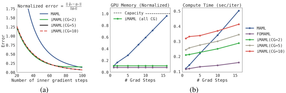
Figure 2: Accuracy, Computation, and Memory tradeoffs of iMAML, MAML, and FOMAML. (a) Metagradient accuracy level in synthetic example. Computed gradients are compared against the exact meta-gradient per Def 3. (b) Computation and memory trade-offs with 4 layer CNN on 20-way-5-shot Omniglot task. We implemented iMAML in PyTorch, and for an apples-to-apples comparison, we use a PyTorch implementation of MAML from: https://github.com/dragen1860/MAML-Pytorch
图 2: iMAML、MAML 和 FOMAML 在准确率、计算量和内存之间的权衡。(a) 合成示例中的元梯度准确度水平。根据定义3将计算梯度与精确元梯度进行比较。(b) 在20类5样本Omniglot任务上使用4层CNN时的计算量与内存权衡。我们使用PyTorch实现了iMAML,为公平对比,采用的PyTorch版MAML实现来自: https://github.com/dragen1860/MAML-Pytorch
Table 2: Omniglot results. MAML results are taken from the original work of Finn et al. [15], and first-order MAML and Reptile results are from Nichol et al. [43]. iMAML with gradient descent (GD) uses 16 and 25 steps for 5-way and 20-way tasks respectively. iMAML with Hessian-free uses $5\mathrm{CG}$ steps to compute the search direction and performs line-search to pick step size. Both versions of iMAML use $\lambda=2.0$ for regular iz ation, and 5 CG steps to compute the task meta-gradient.
| Algorithm | 5-way 1-shot | 5-way 5-shot | 20-way 1-shot | 20-way 5-shot |
| MAML[15] | 98.7±0.4% | 99.9±0.1% | 95.8±0.3% | 98.9 ± 0.2% |
| first-orderMAML[15] | 98.3±0.5% | 99.2 ± 0.2% | 89.4± 0.5% | 97.9 ± 0.1% |
| Reptile [43] | 97.68±0.04% | 99.48±0.06% | 89.43± 0.14% | 97.12±0.32% |
| iMAML,GD (ours) | 99.16±0.35% | 99.67±0.12% | 94.46±0.42% | 98.69 ± 0.1% |
| iMAML,Hessian-Free (ours) | 99.50 ± 0.26% | 99.74 ±0.11% | 96.18±0.36% | 99.14±0.1% |
表 2: Omniglot 实验结果。MAML 结果来自 Finn 等人的原始工作 [15],一阶 MAML 和 Reptile 结果来自 Nichol 等人 [43]。使用梯度下降 (GD) 的 iMAML 在 5-way 和 20-way 任务中分别采用 16 和 25 步。使用无 Hessian 方法的 iMAML 采用 $5\mathrm{CG}$ 步计算搜索方向并通过线搜索选择步长。两个版本的 iMAML 均使用 $\lambda=2.0$ 进行正则化,并采用 5 步 CG 计算任务元梯度。
| 算法 | 5-way 1-shot | 5-way 5-shot | 20-way 1-shot | 20-way 5-shot |
|---|---|---|---|---|
| MAML[15] | 98.7±0.4% | 99.9±0.1% | 95.8±0.3% | 98.9±0.2% |
| 一阶MAML[15] | 98.3±0.5% | 99.2±0.2% | 89.4±0.5% | 97.9±0.1% |
| Reptile[43] | 97.68±0.04% | 99.48±0.06% | 89.43±0.14% | 97.12±0.32% |
| iMAML,GD (本文) | 99.16±0.35% | 99.67±0.12% | 94.46±0.42% | 98.69±0.1% |
| iMAML,无Hessian (本文) | 99.50±0.26% | 99.74±0.11% | 96.18±0.36% | 99.14±0.1% |
The first variant of iMAML we consider involves solving the inner level problem (the regularized objective function in Eq. 4) using gradient descent. The meta-gradient is computed using conjugate gradient, and the meta-parameters are updated using Adam. This presents the most straightforward comparison with MAML, which would follow a similar procedure, but back propagate through the path of optimization as opposed to invoking implicit differentiation. The second variant of iMAML uses a second order method for the inner level problem. In particular, we consider the Hessian-free or Newton-CG [44, 36] method. This method makes a local quadratic approximation to the objective function (in our case, $G(\phi^{\prime},\theta)$ and approximately computes the Newton search direction using CG. Since CG requires only Hessian-vector products, this way of approximating the Newton search direction is scalable to large deep neural networks. The step size can be computed using regular iz ation, damping, trust-region, or linesearch. We use a linesearch on the training loss in our experiments to also illustrate how our method can handle non-differentiable inner optimization loops. We refer the readers to Nocedal & Wright [44] and Martens [36] for a more detailed exposition of this optimization algorithm. Similar approaches have also gained prominence in reinforcement learning [52, 47].
我们考虑的第一种iMAML变体涉及使用梯度下降法解决内层问题(即公式4中的正则化目标函数)。元梯度通过共轭梯度法计算,元参数则采用Adam优化器更新。这为与MAML进行最直接对比提供了基础——虽然MAML会沿优化路径反向传播而非调用隐式微分,但两者遵循相似流程。
第二种iMAML变体采用二阶方法处理内层问题,具体应用了无Hessian矩阵的牛顿-CG法[44,36]。该方法对目标函数(本研究中指$G(\phi^{\prime},\theta)$)进行局部二次逼近,并通过CG近似计算牛顿搜索方向。由于CG仅需Hessian-向量乘积,这种牛顿方向逼近策略可扩展至大型深度神经网络。步长可通过正则化、阻尼、置信域或线搜索确定,实验中我们基于训练损失执行线搜索,以验证方法对不可微内层优化循环的处理能力。详细算法阐述可参阅Nocedal & Wright[44]和Martens[36]的著作,类似方法在强化学习领域[52,47]也取得了显著成效。
Tables 2 and 3 present the results on Omniglot and Mini-ImageNet, respectively. On the Omniglot domain, we find that the GD version of iMAML is competitive with the full MAML algorithm, and subst at i ally better than its approximations (i.e., first-order MAML and Reptile), espe- cially for the harder 20-way tasks. We also find that iMAML with Hessian-free optimization performs substantially better than the other methods, suggesting that powerful optimizers in the inner loop can offer benifits to meta-learning. In the Mini-ImageNet domain, we find that iMAML performs better than MAML and FOMAML. We used $\lambda=0.5$ and 10 gradient steps in the inner loop. We did not perform an extensive hyper parameter sweep, and expect that the results can improve with better hyper parameters. 5 CG steps were used to compute the meta-gradient. The Hessian-free version also uses 5 CG steps for the search direction. Additional experimental details are Appendix F.
表2和表3分别展示了Omniglot和Mini-ImageNet上的实验结果。在Omniglot领域,我们发现iMAML的梯度下降(GD)版本与完整MAML算法表现相当,且明显优于其近似方法(即一阶MAML和Reptile),尤其在更具挑战性的20-way任务中。此外,采用无Hessian优化的iMAML显著优于其他方法,这表明内循环中使用强大的优化器能为元学习带来优势。在Mini-ImageNet领域,iMAML的表现优于MAML和FOMAML。实验采用$\lambda=0.5$的内循环参数,并进行10次梯度步长更新。我们未进行全面的超参数调优,预计通过优化超参数可获得更好结果。元梯度计算使用5次共轭梯度(CG)步长,无Hessian版本同样采用5次CG步长进行方向搜索。其他实验细节见附录F。
Table 3: Mini-ImageNet 5-way-1-shot accuracy
| Algorithm | 5-way 1-shot |
| MAML | 48.70±1.84% |
| first-orderMAML | 48.07 ± 1.75 % |
| Reptile | 49.97± 0.32% |
| iMAML GD (ours) | 48.96 ± 1.84 % |
| iMAML HF (ours) | 49.30 ±1.88 % |
表 3: Mini-ImageNet 5-way-1-shot 准确率
| Algorithm | 5-way 1-shot |
|---|---|
| MAML | 48.70±1.84% |
| first-orderMAML | 48.07 ± 1.75 % |
| Reptile | 49.97± 0.32% |
| iMAML GD (ours) | 48.96 ± 1.84 % |
| iMAML HF (ours) | 49.30 ±1.88 % |
5 Related Work
5 相关工作
Our work considers the general meta-learning problem [51, 55, 41], including few-shot learning [30, 57]. Meta-learning approaches can generally be categorized into metric-learning approaches that learn an embedding space where non-parametric nearest neighbors works well [29, 57, 54, 45, 3], black-box approaches that train a recurrent or recursive neural network to take datapoints as input and produce weight updates [25, 5, 33, 48] or predictions for new inputs [50, 12, 58, 40, 38], and optimization-based approaches that use bi-level optimization to embed learning procedures, such as gradient descent, into the meta-optimization problem [15, 13, 8, 60, 34, 17, 59, 23]. Hybrid approaches have also been considered to combine the benefits of different approaches [49, 56]. We build upon optimization-based approaches, particularly the MAML algorithm [15], which metalearns an initial set of parameters such that gradient-based fine-tuning leads to good generalization. Prior work has considered a number of inner loops, ranging from a very general setting where all parameters are adapted using gradient descent [15], to more structured and specialized settings, such as ridge regression [8], Bayesian linear regression [23], and simulated annealing [2]. The main difference between our work and these approaches is that we show how to analytically derive the gradient of the outer objective without differentiating through the inner learning procedure.
我们的研究考虑了一般元学习问题 [51, 55, 41],包括少样本学习 [30, 57]。元学习方法通常可分为三类:度量学习方法通过学习一个嵌入空间,使非参数最近邻方法表现良好 [29, 57, 54, 45, 3];黑盒方法训练循环或递归神经网络,将数据点作为输入并生成权重更新 [25, 5, 33, 48] 或对新输入的预测 [50, 12, 58, 40, 38];以及基于优化的方法,使用双层优化将学习过程(如梯度下降)嵌入元优化问题中 [15, 13, 8, 60, 34, 17, 59, 23]。也有研究考虑混合方法以结合不同方法的优势 [49, 56]。我们的工作建立在基于优化的方法基础上,特别是 MAML 算法 [15],该算法元学习一组初始参数,使得基于梯度的微调能够实现良好的泛化。先前的研究考虑了多种内部循环设置,从非常通用的场景(所有参数都通过梯度下降调整)[15],到更结构化、专门化的场景,如岭回归 [8]、贝叶斯线性回归 [23] 和模拟退火 [2]。我们的工作与这些方法的主要区别在于,我们展示了如何在不通过内部学习过程求导的情况下,解析地推导外部目标的梯度。
Mathematically, we view optimization-based meta-learning as a bi-level optimization problem. Such problems have been studied in the context of few-shot meta-learning (as discussed previously), gradient-based hyper parameter optimization [35, 46, 19, 11, 10], and a range of other settings [4, 31]. Some prior works have derived implicit gradients for related problems [46, 11, 4] while others propose innovations to aid back-propagation through the optimization path for specific algorithms [35, 19, 24], or approximations like truncation [53]. While the broad idea of implicit differentiation is well known, it has not been empirically demonstrated in the past for learning more than a few parameters (e.g., hyper parameters), or highly structured settings such as quadratic programs [4]. In contrast, our method meta-trains deep neural networks with thousands of parameters. Closest to our setting is the recent work of Lee et al. [32], which uses implicit differentiation for quadratic programs in a final SVM layer. In contrast, our formulation allows for adapting the full network for generic objectives (beyond hinge-loss), thereby allowing for wider applications.
从数学角度看,我们将基于优化的元学习视为双层优化问题。此类问题已在少样本元学习(如前所述)、基于梯度的超参数优化[35, 46, 19, 11, 10]及其他多种场景[4, 31]中被研究。先前工作有的针对相关问题推导了隐式梯度[46, 11, 4],有的则针对特定算法提出改进以辅助通过优化路径的反向传播[35, 19, 24],或采用截断等近似方法[53]。虽然隐式微分的核心思想广为人知,但过去从未在经验上验证过其能学习超过少量参数(如超参数)或高度结构化的场景(如二次规划[4])。相比之下,我们的方法通过元训练实现了具有数千参数的深度神经网络。最接近我们设定的是Lee等人[32]近期的工作,其在最终SVM层对二次规划使用隐式微分。而我们的公式允许为通用目标(超越合页损失)适配整个网络,从而具备更广泛的应用性。
We also note that prior works involving implicit differentiation make a strong assumption of an exact solution in the inner level, thereby providing only asymptotic guarantees. In contrast, we provide finite time guarantees which allows us to analyze the case where the inner level is solved approximately. In practice, the inner level is likely to be solved using iterative optimization algorithms like gradient descent, which only return approximate solutions with finite iterations. Thus, this paper places implicit gradient methods under a strong theoretical footing for practically use.
我们还注意到,先前涉及隐式微分的研究对内部层级的最优解做出了强假设,因此仅能提供渐近性保证。相比之下,我们给出了有限时间保证,这使得我们可以分析内部层级近似求解的情况。实际上,内部层级很可能会使用梯度下降等迭代优化算法求解,这些算法在有限迭代次数下只能返回近似解。因此,本文为隐式梯度方法在实际应用中的使用奠定了坚实的理论基础。
6 Conclusion
6 结论
In this paper, we develop a method for optimization-based meta-learning that removes the need for differentiating through the inner optimization path, allowing us to decouple the outer metagradient computation from the choice of inner optimization algorithm. We showed how this gives us significant gains in compute and memory efficiency, and also conceptually allows us to use a variety of inner optimization methods. While we focused on developing the foundations and theoretical analysis of this method, we believe that this work opens up a number of interesting avenues for future study.
本文提出了一种基于优化的元学习方法,该方法无需对内部优化路径进行微分,从而将外部元梯度计算与内部优化算法的选择解耦。我们证明了该方法能显著提升计算和内存效率,并在概念上支持使用多种内部优化方法。尽管本研究聚焦于该方法的理论基础与分析,但我们相信这项工作为未来研究开辟了多个有价值的方向。
Broader classes of inner loop procedures. While we studied different gradient-based optimization methods in the inner loop, iMAML can in principle be used with a variety of inner loop algorithms, including dynamic programming methods such as $Q$ -learning, two-player adversarial games such as GANs, energy-based models [39], and actor-critic RL methods, and higher-order model-based trajectory optimization methods. This significantly expands the kinds of problems that optimizationbased meta-learning can be applied to.
更广泛的内循环过程类别。虽然我们在内循环中研究了不同的基于梯度的优化方法,但原则上iMAML可以与多种内循环算法结合使用,包括动态规划方法(如$Q$-学习)、双玩家对抗游戏(如GAN)、基于能量的模型[39]、演员-评论家强化学习方法,以及基于高阶模型的轨迹优化方法。这显著扩展了基于优化的元学习所能应用的问题类型。
More flexible regularize rs. We explored one very simple regular iz ation, $\ell_{2}$ regular iz ation to the parameter initialization, which already increases the expressive power over the implicit regular iz ation that MAML provides through truncated gradient descent. To further allow the model to flexibly regularize the inner optimization, a simple extension of iMAML is to learn a vector- or matrix-valued $\lambda$ , which would enable the meta-learner model to co-adapt and co-regularize various parameters of the model. Regularize rs that act on parameterized density functions would also enable meta-learning to be effective for few-shot density estimation.
更灵活的正则化方法。我们探索了一种非常简单的正则化方式,即对参数初始化应用 $\ell_{2}$ 正则化,这已经比MAML通过截断梯度下降提供的隐式正则化增强了表达能力。为了进一步让模型灵活地正则化内部优化过程,iMAML的一个简单扩展是学习一个向量或矩阵形式的 $\lambda$,这将使元学习模型能够协同适应和协同正则化模型的各个参数。作用于参数化密度函数的正则化方法还能让元学习在少样本密度估计中更有效。
Acknowledgements
致谢
Aravind Rajeswaran thanks Emo Todorov for valuable discussions about implicit gradients and potential application domains; Aravind Rajeswaran also thanks Igor Mordatch and Rahul Kidambi for helpful discussions and feedback. Sham Kakade acknowledges funding from the Washington Research Foundation for innovation in Data-intensive Discovery; Sham Kakade also graciously acknowledges support from ONR award N00014-18-1-2247, NSF Award CCF-1703574, and NSF CCF 1740551 award.
Aravind Rajeswaran 感谢 Emo Todorov 关于隐式梯度及其潜在应用领域的有益讨论;同时感谢 Igor Mordatch 和 Rahul Kidambi 的建设性讨论与反馈。Sham Kakade 感谢华盛顿研究基金会 (Washington Research Foundation) 对数据密集型发现创新的资助,并诚挚感谢 ONR 奖项 N00014-18-1-2247、NSF 奖项 CCF-1703574 以及 NSF CCF 1740551 奖项的支持。
References
参考文献
A Relationship between iMAML and Prior Algorithms
iMAML与现有算法的关系
The presented iMAML algorithm has close connections, as well as notable differences, to a number of related algorithms like MAML [15], first-order MAML, and Reptile [43]. Conventionally, these algorithms do not consider any explicit regular iz ation in the inner-level and instead rely on early stopping, through only a few gradient descent steps. In our problem setting described in Eq. 4, we consider an explicitly regularized inner-level problem (refer to discussion in Section 2.2). We describe the connections between the algorithms in this explicitly regularized setting below.
提出的iMAML算法与MAML [15]、一阶MAML和Reptile [43]等相关算法既存在紧密联系,也存在显著差异。传统上,这些算法在内部层级不考虑任何显式正则化,而是仅通过少量梯度下降步骤依赖早停机制。在公式4描述的问题设定中,我们考虑了显式正则化的内部层级问题(参见第2.2节的讨论)。下文将阐述这些算法在显式正则化设定下的关联性。
MAML. The MAML algorithm first invokes an iterative algorithm to solve the inner optimization problem (see definition 1). Subsequently, it back propagates through the path of the optimization algorithm to update the meta-parameters as:
MAML。MAML算法首先调用迭代算法来解决内部优化问题(见定义1),随后通过优化算法的路径进行反向传播,以如下方式更新元参数:
$$
\pmb{\theta}^{k+1}=\pmb{\theta}^{k}-\eta\frac{1}{M}\sum_{i=1}^{M}d_{\theta}\mathcal{L}_ {i}(\mathcal{A}l g_{i}(\pmb{\theta}^{k})).
$$
$$
\pmb{\theta}^{k+1}=\pmb{\theta}^{k}-\eta\frac{1}{M}\sum_{i=1}^{M}d_{\theta}\mathcal{L}_ {i}(\mathcal{A}l g_{i}(\pmb{\theta}^{k})).
$$
Since $\boldsymbol{\mathcal{A}}l g_{i}(\pmb{\theta})$ approximates $\mathcal{A}l g_{i}^{\star}(\pmb\theta)$ , it can be viewed that both MAML and iMAML intend to perform the same idealized update in Eq. 5. However, they perform the meta-gradient computation very differently. MAML back propagates through the path of an iterative algorithm, while iMAML computes the meta-gradient through the implicit Jacobian approach outlined in Section 3.1 (see Figure 1 for a visual depiction). As a result, iMAML can be vastly more efficient in memory while having lesser or comparable computational requirements. It also allows for higher order optimization methods and non-differentiable components.
由于 $\boldsymbol{\mathcal{A}}l g_{i}(\pmb{\theta})$ 逼近 $\mathcal{A}l g_{i}^{\star}(\pmb\theta)$,可以认为MAML和iMAML都试图执行方程5中的理想化更新。但它们在元梯度计算上存在显著差异:MAML通过迭代算法的路径进行反向传播,而iMAML则采用第3.1节所述的隐式雅可比方法计算元梯度 (见图1的可视化说明)。这使得iMAML在内存效率上显著提升,同时保持相当或更低的计算需求,还能支持高阶优化方法和不可微组件。
First-order MAML ignores the effect of meta-parameters $\pmb{\theta}$ on task parameters ${\phi_{i}}$ in the metagradient computation and updates the meta-parameters as:
一阶MAML在元梯度计算中忽略了元参数 $\pmb{\theta}$ 对任务参数 ${\phi_{i}}$ 的影响,并按如下方式更新元参数:
$$
\pmb{\theta}^{k+1}=\pmb{\theta}^{k}-\eta\frac{1}{M}\sum_{i=1}^{M}\nabla_{\phi}\mathcal{L}_ {i}(\phi_{i})\mid_{\phi_{i}=\mathcal{A}l g_{i}(\pmb{\theta}^{k})}
$$
$$
\pmb{\theta}^{k+1}=\pmb{\theta}^{k}-\eta\frac{1}{M}\sum_{i=1}^{M}\nabla_{\phi}\mathcal{L}_ {i}(\phi_{i})\mid_{\phi_{i}=\mathcal{A}l g_{i}(\pmb{\theta}^{k})}
$$
Note that iMAML strictly generalizes this, since first-order MAML is simply iMAML when the conjugate gradient procedure is not invoked (or corresponds to 0 steps of CG). Thus, iMAML allows for an easy way to interpolate from first-order MAML to the full MAML algorithm.
请注意,iMAML严格推广了这一概念,因为当不调用共轭梯度过程(或对应0步CG)时,一阶MAML就是iMAML。因此,iMAML提供了一种简单的方法,可以从一阶MAML过渡到完整的MAML算法。
Reptile [43], similar to first-order MAML, ignores the dependence of task-parameters on metaparameters. However, instead of following the gradients at $\dot{\phi}_ {i}=\mathcal{A}g_{i}(\pmb{\theta}^{k})$ , Reptile uses the taskparameters as targets and slowly moves meta-parameters towards them:
Reptile [43] 与一阶 MAML 类似,忽略了任务参数对元参数的依赖关系。然而,不同于在 $\dot{\phi}_ {i}=\mathcal{A}g_{i}(\pmb{\theta}^{k})$ 处沿梯度更新,Reptile 将任务参数作为目标,并缓慢地将元参数向它们移动:
$$
\pmb{\theta}^{k+1}=\pmb{\theta}^{k}-\eta\frac{1}{M}\sum_{i=1}^{M}(\pmb{\theta}^{k}-\pmb{\phi}_{i}).
$$
$$
\pmb{\theta}^{k+1}=\pmb{\theta}^{k}-\eta\frac{1}{M}\sum_{i=1}^{M}(\pmb{\theta}^{k}-\pmb{\phi}_{i}).
$$
From the proximal point equation in the proof of Lemma 1, we have $\phi_{i}=\theta^{k}-{\textstyle\frac{1}{\lambda}}\nabla_{\phi}{\mathcal{L}}_ {i}(\phi_{i}),$ , using which we see that the Reptile equation becomes: $\begin{array}{r}{\pmb{\theta}^{k+1}=\pmb{\theta}^{k}-\frac{\eta}{\lambda M}\sum_{i=1}^{M}\nabla_{\phi}\mathcal{L}_ {i}(\phi_{i})}\end{array}$ . Thus, Reptile and first-order MAML are identical in our problem formulation up to the choice of learning rate. Making the regular iz ation explicit allows us to illustrate this equivalence.
由引理1证明中的近端点方程可得 $\phi_{i}=\theta^{k}-{\textstyle\frac{1}{\lambda}}\nabla_{\phi}{\mathcal{L}}_ {i}(\phi_{i}),$ ,由此可得Reptile更新方程为: $\begin{array}{r}{\pmb{\theta}^{k+1}=\pmb{\theta}^{k}-\frac{\eta}{\lambda M}\sum_{i=1}^{M}\nabla_{\phi}\mathcal{L}_ {i}(\phi_{i})}\end{array}$ 。因此,在学习率选择相同的情况下,Reptile与一阶MAML (First-order MAML) 在我们的问题表述中完全等价。显式地表达正则化项使我们能够阐明这种等价性。
B Optimization Preliminaries
B 优化基础
Let $f:\mathbb{R}^{d}\rightarrow\mathbb{R}$ . A function $f$ is $B$ Lipschitz (or $B$ -bounded gradient norm) if for all $\boldsymbol{x}\in\mathbb{R}^{d}$
设 $f:\mathbb{R}^{d}\rightarrow\mathbb{R}$。若对所有 $\boldsymbol{x}\in\mathbb{R}^{d}$ 函数 $f$ 满足 $B$ Lipschitz (或 $B$ 有界梯度范数)
$$
\begin{array}{r}{|\nabla f(x)|\leq B.}\end{array}
$$
$$
\begin{array}{r}{|\nabla f(x)|\leq B.}\end{array}
$$
Similarly, we say that a matrix valued function $M:\mathbb{R}^{d}\times\mathbb{R}^{d^{\prime}}\rightarrow\mathbb{R}$ is $\rho$ -Lipschitz if
类似地,我们说矩阵值函数 $M:\mathbb{R}^{d}\times\mathbb{R}^{d^{\prime}}\rightarrow\mathbb{R}$ 是 $\rho$-Lipschitz 的,如果
$$
\left||M(x)-M(x^{\prime})|\right|\leq\rho||x-x^{\prime}||,
$$
$$
\left||M(x)-M(x^{\prime})|\right|\leq\rho||x-x^{\prime}||,
$$
where $|\cdot|$ denotes the spectral norm.
其中 $|\cdot|$ 表示谱范数。
We say that $f$ is $L$ -smooth if for all $x,x^{\prime}\in\mathbb{R}^{d}$
我们说 $f$ 是 $L$-光滑的,如果对于所有 $x,x^{\prime}\in\mathbb{R}^{d}$
$$
||\nabla f(x)-\nabla f(x^{\prime})||\leq L||x-x^{\prime}||
$$
$$
||\nabla f(x)-\nabla f(x^{\prime})||\leq L||x-x^{\prime}||
$$
and that $f$ is $\mu$ -strongly convex if $f$ is convex and if for all $x,x^{\prime}\in\mathbb{R}^{d}$ ,
并且如果函数 $f$ 是凸的,且对于所有 $x,x^{\prime}\in\mathbb{R}^{d}$ 满足 $\mu$ -强凸性条件,
$$
\left||\nabla f(x)-\nabla f(x^{\prime})||\geq\mu||x-x^{\prime}||.\right.
$$
$$
\left||\nabla f(x)-\nabla f(x^{\prime})||\geq\mu||x-x^{\prime}||.\right.
$$
We will make use of the following black-box complexity of first-order gradient methods for minimizing strongly convex and smooth functions.
我们将利用以下一阶梯度方法在黑盒复杂度下最小化强凸且光滑函数。
Lemma 2. ( $\mathit{\check{\Delta}}$ -approximate solver; see $I^{\boldsymbol{9}}\boldsymbol{J},$ Suppose $f$ is a function that is $L$ -smooth and $\mu$ strongly convex. Define $\kappa:=L/\mu,$ , and let $x^{\star}=\operatorname{argmin}f(x)$ . Nesterov’s accelerated gradient descent can be used to find a point $x$ such that:
引理 2. ( $\mathit{\check{\Delta}}$ -近似求解器; 参见 $I^{\boldsymbol{9}}\boldsymbol{J}$ ) 假设函数 $f$ 满足 $L$-光滑且 $\mu$ 强凸性。定义 $\kappa:=L/\mu$ ,并令 $x^{\star}=\operatorname{argmin}f(x)$ 。利用Nesterov加速梯度下降法可找到满足以下条件的点 $x$ :
$$
|x-x^{\star}|\leq\delta
$$
$$
|x-x^{\star}|\leq\delta
$$
using a number of gradient computations of $f$ that is bounded as follows:
使用关于$f$的梯度计算次数,其上限如下:

C Review: Time and Space Complexity of Hessian-Vector Products
C 语言回顾:Hessian-向量积的时间与空间复杂度
We briefly discuss the time and space complexity of Hessian-vector product computation using the reverse mode of automatic differentiation. The reverse mode of automatic differentiation [6, 22] is the widely used method for automatic differentiation in modern software packages like TensorFlow and PyTorch [7]. Recall that for a differentiable function $f(x)$ , the reverse mode of automatic differentiation computes $\nabla f(x)$ in time that is no more than a factor of 5 of the time it takes to compute $f(x)$ itself (see [22] for review). As our algorithm makes use of Hessian vector products, we will make use of the following assumption as to how Hessian vector products will be computed when executing Algorithm 2.
我们简要讨论使用自动微分(automatic differentiation)的反向模式(reverse mode)计算Hessian-向量积的时间和空间复杂度。自动微分的反向模式[6,22]是现代软件包(如TensorFlow和PyTorch[7])中广泛使用的自动微分方法。回顾可微函数$f(x)$,自动微分的反向模式计算$\nabla f(x)$的时间不超过计算$f(x)$本身时间的5倍(详见[22]的综述)。由于我们的算法利用了Hessian向量积,在执行算法2时,我们将对Hessian向量积的计算采用以下假设。
Assumption 1. (Complexity of Hessian-vector product) We assume that the time to compute the Hessian-vector product $\nabla_{\phi}^{2}\hat{\mathcal{L}}_ {i}(\phi)\pmb{v}$ is no more than a (universal) constant over the time used to compute $\nabla\hat{{\mathcal{L}}}_ {i}(\phi)$ (typically, this constant is 5). Furthermore, we assume that the memory used to compute the Hessian-vector product $\nabla_{\phi}^{2}\hat{\mathcal{L}}_ {i}(\phi)\pmb{v}$ is no more than twice the memory used when computing $\nabla\hat{{\mathcal{L}}}_{i}(\phi)$ . This assumption is valid if the reverse mode of automatic differentiation is used to compute Hessian vector products (see [21]).
假设1. (Hessian-vector积的复杂度) 我们假设计算Hessian-vector积$\nabla_{\phi}^{2}\hat{\mathcal{L}}_ {i}(\phi)\pmb{v}$的时间不超过计算$\nabla\hat{{\mathcal{L}}}_ {i}(\phi)$所用时间的(通用)常数倍(通常该常数为5)。此外,我们假设计算Hessian-vector积$\nabla_{\phi}^{2}\hat{\mathcal{L}}_ {i}(\phi)\pmb{v}$的内存消耗不超过计算$\nabla\hat{{\mathcal{L}}}_{i}(\phi)$时的两倍。若使用自动微分的反向模式计算Hessian-vector积,则该假设成立(参见[21])。
A few remarks about this assumption are in order. With regards to computation, first observe that the gradient of the scalar function $\nabla_{\phi}\hat{\mathcal{L}}_ {i}(\phi)^{\top}\pmb{v}$ is the desired Hessian vector product $\nabla_{\phi}^{2}\hat{\mathcal{L}}_ {i}(\phi)\pmb{v}$ . Thus computing the Hessian vector product using the reverse mode is within a constant factor of computing the function itself, which is simply the cost of computing $\nabla\hat{\mathcal{L}}_ {i}(\phi)^{\top}\pmb{v}$ . The issue of memory is more subtle (see [21]), which we now discuss. The memory used to compute the gradient of a scalar cost function $f(x)$ using the reverse mode of auto-differentiation is proportional to the size of the computation graph; precisely, the memory required to compute the gradient is equal to the total space required to store all the intermediate variables used when computing $f(x)$ . In practice, this is often much larger than the memory required to compute $f(x)$ itself, due to that all intermediate variables need not be simultaneously stored in memory when computing $f(x)$ . However, for the special case of computing the gradient of the function $f(\phi)=\nabla_{\phi}\hat{\mathcal{L}}_ {i}(\phi)^{\top}v$ , the factor of 2 in the memory bound is a consequence of the following reason: first, using the reverse mode to compute $f(\phi)$ means we already have stored the computation graph of $\hat{\mathcal{L}}_ {i}(\phi)$ itself. Furthermore, the size of the computation graph for computing $f(\phi)=\nabla_{\phi}\hat{\mathcal{L}}_ {i}(\phi)^{\top}v$ is essentially the same size as the computation graph of $\hat{\mathcal{L}}_{i}(\phi)$ . This leads to the factor of 2 memory bound; see Griewank [21] for further discussion.
关于这一假设有几点需要说明。在计算方面,首先注意到标量函数的梯度 $\nabla_{\phi}\hat{\mathcal{L}}_ {i}(\phi)^{\top}\pmb{v}$ 正是所需的Hessian向量积 $\nabla_{\phi}^{2}\hat{\mathcal{L}}_ {i}(\phi)\pmb{v}$。因此,使用反向模式计算Hessian向量积的代价与计算函数本身仅相差一个常数因子,即仅需计算 $\nabla\hat{\mathcal{L}}_{i}(\phi)^{\top}\pmb{v}$ 的成本。内存问题则更为微妙(见[21]),现讨论如下:
采用自动微分反向模式计算标量代价函数 $f(x)$ 梯度时,内存消耗与计算图大小成正比;具体而言,计算梯度所需内存等于存储计算 $f(x)$ 时所有中间变量的总空间。实践中,由于计算 $f(x)$ 时无需同时将所有中间变量存储在内存中,该内存需求通常远大于计算 $f(x)$ 本身所需内存。
然而,对于计算函数 $f(\phi)=\nabla_{\phi}\hat{\mathcal{L}}_ {i}(\phi)^{\top}v$ 梯度的特殊情况,内存限制出现2倍系数的原因如下:首先,使用反向模式计算 $f(\phi)$ 意味着已存储 $\hat{\mathcal{L}}_ {i}(\phi)$ 的计算图;此外,计算 $f(\phi)=\nabla_{\phi}\hat{\mathcal{L}}_ {i}(\phi)^{\top}v$ 的图规模本质上与 $\hat{\mathcal{L}}_{i}(\phi)$ 的计算图相同。这导致了2倍的内存限制系数,详见Griewank [21]的进一步讨论。
D Additional Discussion About Compute and Memory Complexity
D 关于计算与内存复杂度的补充讨论
Our main complexity results are summarized in Table 1. For these results, we consider two notions of error that are subtly different, which we explicitly define below. Let ${\mathbf{}}_ {}{\mathbf{}}_ {3}{\mathbf{}}_ {i}$ be the computed metagradient for task $\tau_{i}$ . Then, the errors we consider are:
我们的主要复杂度结果总结在表1中。对于这些结果,我们考虑了两种存在微妙差异的误差定义,具体如下:设${\mathbf{}}_ {}{\mathbf{}}_ {3}{\mathbf{}}_ {i}$为任务$\tau_{i}$的计算元梯度,则我们考察的误差为:
Definition 3. Exact-solve error (our notion of error): Our goal is to accurately compute the gradient of $F(\theta)$ as defined in Equation 4, where $\boldsymbol{\mathcal{A}}\boldsymbol{l}\boldsymbol{g}_ {i}^{\star}(\boldsymbol{\theta})$ is an exact algorithm. Specifically, we seek to compute a ${\mathbf{}}_ {}{\mathbf{}}_ {3}{\mathbf{}}_{i}$ such that:
定义3. 精确求解误差(我们的误差概念): 我们的目标是准确计算方程4中定义的$F(\theta)$的梯度,其中$\boldsymbol{\mathcal{A}}\boldsymbol{l}\boldsymbol{g}_ {i}^{\star}(\boldsymbol{\theta})$是一个精确算法。具体而言,我们需要计算满足以下条件的${\mathbf{}}_ {}{\mathbf{}}_ {3}{\mathbf{}}_{i}$:
$$
\begin{array}{r}{|\pmb{g}_ {i}-d_{\theta}\mathcal{L}_ {i}(\mathcal{A}l g_{i}^{\star}(\pmb{\theta}))|\le\epsilon}\end{array}
$$
$$
\begin{array}{r}{|\pmb{g}_ {i}-d_{\theta}\mathcal{L}_ {i}(\mathcal{A}l g_{i}^{\star}(\pmb{\theta}))|\le\epsilon}\end{array}
$$
where $\epsilon$ is the error in the gradient computation.
其中 $\epsilon$ 是梯度计算中的误差。
Definition 4. Approx-solve error: Here we suppose that $\boldsymbol{\mathcal{A}}\boldsymbol{l}_ {\boldsymbol{\mathit{g}}_ {i}}$ computes a $\delta$ –accurate solution to the inner optimization problem over $G_{i}$ in Eq. 4, i.e. that $\boldsymbol{\mathcal{A}}\boldsymbol{l}_ {\boldsymbol{\mathit{g}}_ {i}}$ satisfies $\lVert\mathcal{A}l g_{i}({\pmb\theta})-\mathcal{A}l g_{i}^{\star}({\pmb\theta})\rVert\le\delta$ , as per definition 1. Then the objective is to compute a $\pmb{g}$ such that:
定义 4. 近似求解误差: 这里我们假设 $\boldsymbol{\mathcal{A}}\boldsymbol{l}_ {\boldsymbol{\mathit{g}}_ {i}}$ 计算得到式 4 中关于 $G_{i}$ 的内部优化问题的 $\delta$ 精度解, 即 $\boldsymbol{\mathcal{A}}\boldsymbol{l}_ {\boldsymbol{\mathit{g}}_ {i}}$ 满足 $\lVert\mathcal{A}l g_{i}({\pmb\theta})-\mathcal{A}l g_{i}^{\star}({\pmb\theta})\rVert\le\delta$, 根据定义 1。那么目标是计算一个 $\pmb{g}$ 使得:
$$
|{\pmb g}-d_{\theta}\mathcal{L}_ {i}(A l g_{i}(\pmb\theta))|\le\epsilon
$$
$$
|{\pmb g}-d_{\theta}\mathcal{L}_ {i}(A l g_{i}(\pmb\theta))|\le\epsilon
$$
where ϵ is the error in the gradient computation of $d_{\theta}\mathscr{L}_ {i}({\mathcal{A}}l g_{i}(\pmb{\theta}))$ . Subtly, note that the gradient is with respect to the $\delta$ -approximate algorithm, as opposed to using $\boldsymbol{\mathcal{A}}\boldsymbol{l}\boldsymbol{g}_{i}^{\star}$ .
其中,ϵ是梯度计算$d_{\theta}\mathscr{L}_ {i}({\mathcal{A}}l g_{i}(\pmb{\theta}))$的误差。需要特别注意的是,这里的梯度是针对δ近似算法计算的,而非使用$\boldsymbol{\mathcal{A}}\boldsymbol{l}\boldsymbol{g}_{i}^{\star}$。
For the complexity results, we assume that MAML invokes $\boldsymbol{\mathcal{A}}\boldsymbol{l}_ {\boldsymbol{\mathit{g}}_ {i}}$ to get a $\delta$ -approximate solution for inner problem (recall definition 1). The exact-solve error for MAML is not known in the literature; in particular, even as $\delta\rightarrow0$ it is not evident if the approx-solve solution tends to the exact-solve solution, unless further regularity conditions are imposed. The approx-solve error for MAML is 0, ignoring finite-precision and numerical issues, since it back propagates through the path. Truncated backprop [53] also invokes $\boldsymbol{\mathcal{A}}\boldsymbol{l}_ {\boldsymbol{\mathit{g}}_ {i}}$ to obtain a $\delta$ -approximate solution but instead performs a truncated or partial back-propagation so that it uses a smaller number of iterations when computing the gradient through the path of $\boldsymbol{\mathcal{A}}l g_{i}(\pmb{\theta})$ . Exact-solve error for truncated backprop is also not known, but a small approx-solve error can be obtained with less memory than full back-prop. We use Prop 3.1 of Shaban et al. [53] to provide a guarantee that leads to an $\epsilon$ –accurate approximation of the full-backprop (i.e. MAML) gradient. It is not evident how accurate the truncated procedure is when an accelerated method is used instead. Finally, our iMAML algorithm also invokes an approximate solver $\boldsymbol{\mathcal{A}}\boldsymbol{l}_ {\boldsymbol{\mathit{g}}_ {i}}$ rather than $\boldsymbol{\mathcal{A}}\boldsymbol{l}g_{i}^{\star}$ . However, importantly, we guarantee a small exact-solve error even though we do not require access to $\boldsymbol{\mathcal{A}}\boldsymbol{l}g_{i}^{\star}$ . Furthermore, the iMAML algorithm also requires substantially less memory. Up to small constant factors, it only utilizes the memory required for computing a single gradient of $\hat{\mathcal{L}}_{i}(\cdot)$ .
关于复杂度结果,我们假设MAML调用$\boldsymbol{\mathcal{A}}\boldsymbol{l}_ {\boldsymbol{\mathit{g}}_ {i}}$来获得内层问题的$\delta$近似解(参见定义1)。文献中尚未明确MAML的精确求解误差;特别是当$\delta\rightarrow0$时,除非施加额外的正则条件,否则近似解是否趋近于精确解尚不明确。MAML的近似求解误差为0(忽略有限精度和数值问题),因为它沿路径反向传播。截断反向传播[53]同样调用$\boldsymbol{\mathcal{A}}\boldsymbol{l}_ {\boldsymbol{\mathit{g}}_ {i}}$来获得$\delta$近似解,但执行截断或部分反向传播,从而在通过$\boldsymbol{\mathcal{A}}l g_{i}(\pmb{\theta})$路径计算梯度时使用更少的迭代次数。截断反向传播的精确求解误差亦未可知,但能以比完整反向传播更少的内存获得较小的近似求解误差。我们采用Shaban等人[53]的命题3.1来保证其能实现$\epsilon$精度的完整反向传播(即MAML)梯度近似。当使用加速方法时,截断过程的精度尚不明确。最后,我们的iMAML算法同样调用近似求解器$\boldsymbol{\mathcal{A}}\boldsymbol{l}_ {\boldsymbol{\mathit{g}}_ {i}}$而非$\boldsymbol{\mathcal{A}}\boldsymbol{l}g_{i}^{\star}$。但关键的是,我们保证了较小的精确求解误差,且无需访问$\boldsymbol{\mathcal{A}}\boldsymbol{l}g_{i}^{\star}$。此外,iMAML算法的内存需求显著降低——在微小常数因子范围内,仅需计算$\hat{\mathcal{L}}_{i}(\cdot)$单个梯度所需的内存。
E Proofs
E 证明
Lemma 1, restated. Consider $\mathcal{A}l g_{i}^{\star}(\pmb\theta)$ as defined in Eq. 4 for task $\tau_{i}$ . Let $\phi_{i}=\mathcal{A}l g_{i}^{\star}(\pmb\theta)$ be the result of $\mathcal{A}l g_{i}^{\star}(\pmb\theta)$ . If $\begin{array}{r}{\left(I+\frac{1}{\lambda}\nabla_{\phi}^{2}\hat{\mathcal{L}}_ {i}(\phi_{i})\right)}\end{array}$ is invertible, then the derivative Jacobian is
引理1 (重述). 考虑任务$\tau_{i}$中由公式4定义的$\mathcal{A}l g_{i}^{\star}(\pmb\theta)$。设$\phi_{i}=\mathcal{A}l g_{i}^{\star}(\pmb\theta)$为$\mathcal{A}l g_{i}^{\star}(\pmb\theta)$的结果。若$\begin{array}{r}{\left(I+\frac{1}{\lambda}\nabla_{\phi}^{2}\hat{\mathcal{L}}_ {i}(\phi_{i})\right)}\end{array}$可逆,则导数雅可比矩阵为
$$
\frac{d\mathcal{A}l g_{i}^{\star}(\pmb\theta)}{d\pmb\theta}=\left(\pmb I+\frac{1}{\lambda}\nabla_{\phi}^{2}\hat{\mathcal{L}}_ {i}(\phi_{i})\right)^{-1}.
$$
$$
\frac{d\mathcal{A}l g_{i}^{\star}(\pmb\theta)}{d\pmb\theta}=\left(\pmb I+\frac{1}{\lambda}\nabla_{\phi}^{2}\hat{\mathcal{L}}_ {i}(\phi_{i})\right)^{-1}.
$$
Proof. We drop the task $i$ subscripts in the proof for convenience. Since $\phi=\mathcal{A}l g^{\star}(\pmb\theta)$ is the minimizer of $G(\phi^{\prime},\theta)$ in Eq. 4, the stationary point conditions imply that
证明。为方便起见,我们在证明中省略任务$i$的下标。由于$\phi=\mathcal{A}l g^{\star}(\pmb\theta)$是式4中$G(\phi^{\prime},\theta)$的最小值点,其驻点条件表明
$$
\nabla_{\phi^{\prime}}G(\phi^{\prime},\theta)\mid_{\phi^{\prime}=\phi}=0\implies\nabla\hat{\mathcal{L}}(\phi)+\lambda(\phi-\theta)=0\implies\phi=\theta-\frac{1}{\lambda}\nabla\hat{\mathcal{L}}(\phi),
$$
$$
\nabla_{\phi^{\prime}}G(\phi^{\prime},\theta)\mid_{\phi^{\prime}=\phi}=0\implies\nabla\hat{\mathcal{L}}(\phi)+\lambda(\phi-\theta)=0\implies\phi=\theta-\frac{1}{\lambda}\nabla\hat{\mathcal{L}}(\phi),
$$
which is an implicit equation that often arises in proximal point methods. When the derivative exists, we can differentiate the above equation to obtain:
这是一个在近端点方法中经常出现的隐式方程。当导数存在时,我们可以对上述方程进行微分得到:
$$
\frac{d\phi}{d\theta}=I-\frac{1}{\lambda}\nabla^{2}\hat{\mathcal{L}}(\phi)\frac{d\phi}{d\theta}\implies\left(I+\frac{1}{\lambda}\nabla^{2}\hat{\mathcal{L}}(\phi)\right)\frac{d\phi}{d\theta}=I.
$$
$$
\frac{d\phi}{d\theta}=I-\frac{1}{\lambda}\nabla^{2}\hat{\mathcal{L}}(\phi)\frac{d\phi}{d\theta}\implies\left(I+\frac{1}{\lambda}\nabla^{2}\hat{\mathcal{L}}(\phi)\right)\frac{d\phi}{d\theta}=I.
$$
which completes the proof.
证明完毕。
Recall that:
回想一下:
$$
G_{i}(\phi^{\prime},\theta):=\hat{\mathcal{L}}_{i}(\phi^{\prime})+\frac{\lambda}{2}||\phi^{\prime}-\theta||^{2}.
$$
$$
G_{i}(\phi^{\prime},\theta):=\hat{\mathcal{L}}_{i}(\phi^{\prime})+\frac{\lambda}{2}||\phi^{\prime}-\theta||^{2}.
$$
Assumption 2. (Regularity conditions) Suppose the following holds for all tasks $i$ :
假设2. (正则性条件) 假设以下条件对所有任务$i$成立:
- $\mathcal{L}_{i}(\cdot)$ is $B$ Lipshitz and $L$ smooth.
- $\mathcal{L}_{i}(\cdot)$ 是 $B$ Lipschitz 且 $L$ 光滑的。
- For all θ, $G_{i}(\cdot,\pmb\theta)$ is both a $\beta$ -smooth function and a $\mu$ -strongly convex function. Define:
- 对于所有θ,$G_{i}(\cdot,\pmb\theta)$既是$\beta$平滑函数,又是$\mu$强凸函数。定义:
$$
\kappa:=\frac{\beta}{\mu}.
$$
$$
\kappa:=\frac{\beta}{\mu}.
$$
- $\hat{\mathcal{L}}_ {i}(\cdot)$ is $\rho$ -Lipshitz Hessian, i.e. $\nabla^{2}\hat{\mathcal{L}}_{i}(\cdot)$ is $\rho$ -Lipshitz.
- $\hat{\mathcal{L}}_ {i}(\cdot)$ 是 $\rho$-Lipschitz Hessian,即 $\nabla^{2}\hat{\mathcal{L}}_{i}(\cdot)$ 满足 $\rho$-Lipschitz 连续性。
- For all θ, suppose the arg-minimizer of $G_{i}(\cdot,\pmb\theta)$ is unique and bounded in a ball of radius $D$ , i.e. for all $\pmb{\theta}$ ,
- 对于所有θ,假设 $G_{i}(\cdot,\pmb\theta)$ 的arg-minimizer在半径为 $D$ 的球内唯一且有界,即对于所有 $\pmb{\theta}$ ,
$$
|\mathcal{A}l g_{i}^{\star}(\pmb\theta)|\leq D.
$$
$$
|\mathcal{A}l g_{i}^{\star}(\pmb\theta)|\leq D.
$$
Lemma 3. (Implicit Gradient Accuracy) Suppose Assumption 2 holds. Fix a task i. Suppose that $\phi_{i}$ satisfies:
引理3. (隐式梯度精度) 假设假设2成立。固定任务i。假设 $\phi_{i}$ 满足:
$$
\lVert\phi_{i}-\mathcal{A}l g_{i}^{\star}(\pmb\theta)\rVert\leq\delta
$$
$$
\lVert\phi_{i}-\mathcal{A}l g_{i}^{\star}(\pmb\theta)\rVert\leq\delta
$$
and that ${\mathbf{}}_ {}{\mathbf{}}_ {3}{\mathbf{}}_{i}$ satisfies:
且 ${\mathbf{}}_ {}{\mathbf{}}_ {3}{\mathbf{}}_{i}$ 满足:
$$
\lVert g_{i}-\left(I+\frac{1}{\lambda}\nabla^{2}\hat{\mathcal L}_ {i}(\phi)\right)^{-1}\nabla_{\phi}\mathcal L_{i}(\phi)\rVert\leq\delta^{\prime}.
$$
$$
\lVert g_{i}-\left(I+\frac{1}{\lambda}\nabla^{2}\hat{\mathcal L}_ {i}(\phi)\right)^{-1}\nabla_{\phi}\mathcal L_{i}(\phi)\rVert\leq\delta^{\prime}.
$$
Assuming that $\delta<\mu/(2\rho)$ , we have that:
假设 $\delta<\mu/(2\rho)$,则有:
$$
|{\boldsymbol{g}}_ {i}-d_{\theta}\mathcal{L}_ {i}(\mathcal{A}l g_{i}^{\star}(\pmb{\theta}))|\leq\left(2\frac{\lambda\rho}{\mu^{2}}B+\frac{\lambda L}{\mu}\right)\delta+\delta^{\prime}
$$
$$
|{\boldsymbol{g}}_ {i}-d_{\theta}\mathcal{L}_ {i}(\mathcal{A}l g_{i}^{\star}(\pmb{\theta}))|\leq\left(2\frac{\lambda\rho}{\mu^{2}}B+\frac{\lambda L}{\mu}\right)\delta+\delta^{\prime}
$$
Proof. First, observe that:
证明。首先,观察到:
$$
d_{\theta}\mathcal{L}_ {i}(\mathcal{A}l g_{i}^{\star}(\theta))=\left(I+\frac{1}{\lambda}\nabla^{2}\hat{\mathcal{L}}_ {i}(\mathcal{A}l g_{i}^{\star}(\theta))\right)^{-1}\nabla_{\phi}\mathcal{L}_ {i}(\mathcal{A}l g_{i}^{\star}(\theta))
$$
$$
d_{\theta}\mathcal{L}_ {i}(\mathcal{A}l g_{i}^{\star}(\theta))=\left(I+\frac{1}{\lambda}\nabla^{2}\hat{\mathcal{L}}_ {i}(\mathcal{A}l g_{i}^{\star}(\theta))\right)^{-1}\nabla_{\phi}\mathcal{L}_ {i}(\mathcal{A}l g_{i}^{\star}(\theta))
$$
For notational convenience, we drop the $i$ subscripts within the proof. We have:
为便于标记,我们在证明中省略下标$i$。可得:
$$
\begin{array}{r l}&{|d_{\theta}\mathcal{L}(\mathcal{A}l g^{\star}(\theta))-g|}\ {\le}&{|d_{\theta}\mathcal{L}(\mathcal{A}l g^{\star}(\theta))-\left(I+\displaystyle\frac{1}{\lambda}\nabla^{2}\hat{\mathcal{L}}(\phi)\right)^{-1}\nabla_{\phi}\mathcal{L}(\phi)|+\delta^{\prime}}\ {\le}&{|d_{\theta}\mathcal{L}(\mathcal{A}l g^{\star}(\theta))-\left(I+\displaystyle\frac{1}{\lambda}\nabla^{2}\hat{\mathcal{L}}(\phi)\right)^{-1}\nabla_{\phi}\mathcal{L}(\mathcal{A}l g^{\star}(\theta))|+}\ &{|\left(I+\displaystyle\frac{1}{\lambda}\nabla^{2}\hat{\mathcal{L}}(\phi)\right)^{-1}(\nabla_{\phi}\mathcal{L}(\mathcal{A}l g^{\star}(\theta))-\nabla_{\phi}\mathcal{L}(\phi))|+\delta^{\prime}}\end{array}
$$
$$
\begin{array}{r l}&{|d_{\theta}\mathcal{L}(\mathcal{A}l g^{\star}(\theta))-g|}\ {\le}&{|d_{\theta}\mathcal{L}(\mathcal{A}l g^{\star}(\theta))-\left(I+\displaystyle\frac{1}{\lambda}\nabla^{2}\hat{\mathcal{L}}(\phi)\right)^{-1}\nabla_{\phi}\mathcal{L}(\phi)|+\delta^{\prime}}\ {\le}&{|d_{\theta}\mathcal{L}(\mathcal{A}l g^{\star}(\theta))-\left(I+\displaystyle\frac{1}{\lambda}\nabla^{2}\hat{\mathcal{L}}(\phi)\right)^{-1}\nabla_{\phi}\mathcal{L}(\mathcal{A}l g^{\star}(\theta))|+}\ &{|\left(I+\displaystyle\frac{1}{\lambda}\nabla^{2}\hat{\mathcal{L}}(\phi)\right)^{-1}(\nabla_{\phi}\mathcal{L}(\mathcal{A}l g^{\star}(\theta))-\nabla_{\phi}\mathcal{L}(\phi))|+\delta^{\prime}}\end{array}
$$
where the first inequality uses the triangle inequality.
第一个不等式使用了三角不等式。
We now bound each of these terms. For the second term,
我们现在来界定每一项的范围。对于第二项,
$$
\begin{array}{r l}&{\parallel\left(I+\frac{1}{\lambda}\nabla^{2}\hat{\mathcal{L}}(\phi)\right)^{-1}\left(\nabla_{\phi}\mathcal{L}(\boldsymbol{\mathcal{A}}l g^{\star}(\theta))-\nabla_{\phi}\mathcal{L}(\phi)\right)\parallel}\ {\leq}&{\parallel\left(I+\frac{1}{\lambda}\nabla^{2}\hat{\mathcal{L}}(\phi)\right)^{-1}\parallel\parallel\nabla_{\phi}\mathcal{L}(\boldsymbol{\mathcal{A}}l g^{\star}(\theta))-\nabla_{\phi}\mathcal{L}(\phi)\parallel}\ {\leq}&{\lambda L\parallel\left(\lambda I+\nabla^{2}\hat{\mathcal{L}}(\phi)\right)^{-1}\parallel\parallel\boldsymbol{\mathcal{A}}l g^{\star}(\theta)-\phi\parallel}\ {=}&{\lambda L\parallel\nabla_{\phi}^{2}G(\phi,\theta)^{-1}\parallel\parallel\boldsymbol{\mathcal{A}}l g^{\star}(\theta)-\phi\parallel}\ {\leq}&{\frac{\lambda L}{\mu}\delta}\end{array}
$$
$$
\begin{array}{r l}&{\parallel\left(I+\frac{1}{\lambda}\nabla^{2}\hat{\mathcal{L}}(\phi)\right)^{-1}\left(\nabla_{\phi}\mathcal{L}(\boldsymbol{\mathcal{A}}l g^{\star}(\theta))-\nabla_{\phi}\mathcal{L}(\phi)\right)\parallel}\ {\leq}&{\parallel\left(I+\frac{1}{\lambda}\nabla^{2}\hat{\mathcal{L}}(\phi)\right)^{-1}\parallel\parallel\nabla_{\phi}\mathcal{L}(\boldsymbol{\mathcal{A}}l g^{\star}(\theta))-\nabla_{\phi}\mathcal{L}(\phi)\parallel}\ {\leq}&{\lambda L\parallel\left(\lambda I+\nabla^{2}\hat{\mathcal{L}}(\phi)\right)^{-1}\parallel\parallel\boldsymbol{\mathcal{A}}l g^{\star}(\theta)-\phi\parallel}\ {=}&{\lambda L\parallel\nabla_{\phi}^{2}G(\phi,\theta)^{-1}\parallel\parallel\boldsymbol{\mathcal{A}}l g^{\star}(\theta)-\phi\parallel}\ {\leq}&{\frac{\lambda L}{\mu}\delta}\end{array}
$$
where we the second inequality uses that $\nabla_{\phi}\mathcal{L}$ is $L$ -smooth and the final inequality uses that $G$ is $\mu$ strongly convex.
其中第二个不等式利用了 $\nabla_{\phi}\mathcal{L}$ 的 $L$ -光滑性,最后一个不等式则基于 $G$ 的 $\mu$ 强凸性。
For the first term, we have:
对于第一项,我们有:
$$
\begin{array}{r l}&{|d_{\theta}\mathcal{L}(\mathcal{A}l g^{\star}(\theta))-\left(I+\displaystyle\frac{1}{\lambda}\nabla^{2}\hat{\mathcal{L}}(\phi)\right)^{-1}\nabla_{\phi}\mathcal{L}(\mathcal{A}l g^{\star}(\theta))|}\ {=}&{|\left(\left(I+\displaystyle\frac{1}{\lambda}\nabla^{2}\hat{\mathcal{L}}(\mathcal{A}l g^{\star}(\theta))\right)^{-1}-\left(I+\displaystyle\frac{1}{\lambda}\nabla^{2}\hat{\mathcal{L}}(\phi)\right)^{-1}\right)\nabla_{\phi}\mathcal{L}(\mathcal{A}l g^{\star}(\theta))|}\ {\leq}&{\lambda|\left(\lambda I+\nabla^{2}\hat{\mathcal{L}}(\mathcal{A}l g^{\star}(\theta))\right)^{-1}-\left(\lambda I+\nabla^{2}\hat{\mathcal{L}}(\phi)\right)^{-1}|B,}\end{array}
$$
$$
\begin{array}{r l}&{|d_{\theta}\mathcal{L}(\mathcal{A}l g^{\star}(\theta))-\left(I+\displaystyle\frac{1}{\lambda}\nabla^{2}\hat{\mathcal{L}}(\phi)\right)^{-1}\nabla_{\phi}\mathcal{L}(\mathcal{A}l g^{\star}(\theta))|}\ {=}&{|\left(\left(I+\displaystyle\frac{1}{\lambda}\nabla^{2}\hat{\mathcal{L}}(\mathcal{A}l g^{\star}(\theta))\right)^{-1}-\left(I+\displaystyle\frac{1}{\lambda}\nabla^{2}\hat{\mathcal{L}}(\phi)\right)^{-1}\right)\nabla_{\phi}\mathcal{L}(\mathcal{A}l g^{\star}(\theta))|}\ {\leq}&{\lambda|\left(\lambda I+\nabla^{2}\hat{\mathcal{L}}(\mathcal{A}l g^{\star}(\theta))\right)^{-1}-\left(\lambda I+\nabla^{2}\hat{\mathcal{L}}(\phi)\right)^{-1}|B,}\end{array}
$$
using that $\nabla_{\phi}\mathcal{L}$ is $B$ Lipshitz. Now let
利用 $\nabla_{\phi}\mathcal{L}$ 是 $B$ Lipschitz 的这一性质。现在设
$$
\Delta:=\nabla^{2}\hat{\mathcal{L}}(\mathcal{A}l g^{\star}(\pmb{\theta}))-\nabla^{2}\hat{\mathcal{L}}(\phi),\quad M:=\nabla_{\phi}^{2}G(\phi,\pmb{\theta})=\lambda I+\nabla^{2}\hat{\mathcal{L}}(\phi)
$$
$$
\Delta:=\nabla^{2}\hat{\mathcal{L}}(\mathcal{A}l g^{\star}(\pmb{\theta}))-\nabla^{2}\hat{\mathcal{L}}(\phi),\quad M:=\nabla_{\phi}^{2}G(\phi,\pmb{\theta})=\lambda I+\nabla^{2}\hat{\mathcal{L}}(\phi)
$$
Due to that $\nabla^{2}\hat{\mathcal{L}}(\cdot)$ is Lipshitz Hessian, $|\Delta|\le\rho\delta$ . Also, by our assumption on $\delta$ , we have that:
由于 $\nabla^{2}\hat{\mathcal{L}}(\cdot)$ 满足 Lipschitz Hessian 条件,故 $|\Delta|\le\rho\delta$ 。此外,根据我们对 $\delta$ 的假设可得:
$$
|M^{-1}\Delta|\le|\Delta|/\mu\le\rho\delta/\mu\le1/2,
$$
$$
|M^{-1}\Delta|\le|\Delta|/\mu\le\rho\delta/\mu\le1/2,
$$
which implies that $\left|\left(I+M^{-1}\Delta\right)^{-1}\right|\leq2$ . Hence,
这意味着 $\left|\left(I+M^{-1}\Delta\right)^{-1}\right|\leq2$ 。因此,
$$
\begin{array}{r l}&{\Vert\left(\lambda I+\nabla^{2}\hat{\mathcal{L}}(\mathcal{A}l g^{\star}(\theta))\right)^{-1}-\left(\lambda I+\nabla^{2}\hat{\mathcal{L}}(\phi)\right)^{-1}\Vert}\ {=}&{\Vert\left(M+\Delta\right)^{-1}-M^{-1}\Vert}\ {\leq}&{\Vert M^{-1}\Vert\Vert\left(I+M^{-1}\Delta\right)^{-1}-I\Vert}\ {=}&{\Vert M^{-1}\Vert\Vert\left(I+M^{-1}\Delta\right)^{-1}\left(I-\left(I+M^{-1}\Delta\right)\right)\Vert}\ {\leq}&{\Vert M^{-1}\Vert\Vert\left(I+M^{-1}\Delta\right)^{-1}\Vert\Vert M^{-1}\Delta\Vert}\ {\leq}&{\frac{1}{\mu}\cdot2\cdot\frac{\rho\delta}{\mu}=2\frac{\rho}{\mu^{2}}\delta.}\end{array}
$$
$$
\begin{array}{r l}&{\Vert\left(\lambda I+\nabla^{2}\hat{\mathcal{L}}(\mathcal{A}l g^{\star}(\theta))\right)^{-1}-\left(\lambda I+\nabla^{2}\hat{\mathcal{L}}(\phi)\right)^{-1}\Vert}\ {=}&{\Vert\left(M+\Delta\right)^{-1}-M^{-1}\Vert}\ {\leq}&{\Vert M^{-1}\Vert\Vert\left(I+M^{-1}\Delta\right)^{-1}-I\Vert}\ {=}&{\Vert M^{-1}\Vert\Vert\left(I+M^{-1}\Delta\right)^{-1}\left(I-\left(I+M^{-1}\Delta\right)\right)\Vert}\ {\leq}&{\Vert M^{-1}\Vert\Vert\left(I+M^{-1}\Delta\right)^{-1}\Vert\Vert M^{-1}\Delta\Vert}\ {\leq}&{\frac{1}{\mu}\cdot2\cdot\frac{\rho\delta}{\mu}=2\frac{\rho}{\mu^{2}}\delta.}\end{array}
$$
The proof is completed by substitution.
证明通过代入完成。
Theorem 2. (Approximate Implicit Gradient Computation) Suppose Assumption 2 holds. Fix a task i. Let
定理2. (近似隐式梯度计算) 假设假设2成立。固定任务i。令
$$
B_{1}:=2\frac{\lambda\rho}{\mu^{2}}B+\frac{\lambda L}{\mu}
$$
$$
B_{1}:=2\frac{\lambda\rho}{\mu^{2}}B+\frac{\lambda L}{\mu}
$$
Suppose Nesterov’s accelerated gradient descent algorithm is used to compute $\phi$ (as desired in Algorithm 2), using a number of iterations that is:
假设使用Nesterov加速梯度下降算法来计算$\phi$(如算法2所期望的),采用的迭代次数为:
$$
2\sqrt{\kappa}\log\left(8\kappa D\left(\frac{B_{1}}{\epsilon}+\frac{\rho}{\mu}\right)\right)
$$
$$
2\sqrt{\kappa}\log\left(8\kappa D\left(\frac{B_{1}}{\epsilon}+\frac{\rho}{\mu}\right)\right)
$$
and suppose Nesterov’s accelerated gradient descent algorithm (or the conjugate gradient algorithm 1) is used to compute ${\mathbf{}}_ {}{\mathbf{}}_ {3}{\mathbf{}}_{i}$ using a number of iterations that is:
假设使用Nesterov加速梯度下降算法(或共轭梯度算法1)来计算 ${\mathbf{}}_ {}{\mathbf{}}_ {3}{\mathbf{}}_{i}$,所需迭代次数为:
$$
2\sqrt{\kappa}\log\left(4\kappa{\frac{(\lambda/\mu)B}{\epsilon}}\right).
$$
$$
2\sqrt{\kappa}\log\left(4\kappa{\frac{(\lambda/\mu)B}{\epsilon}}\right).
$$
We have that:
我们有:
$$
\begin{array}{r}{|\pmb{g}_ {i}-d_{\theta}\mathcal{L}_ {i}(A l g_{i}^{\star}(\pmb{\theta}))|\le\epsilon.}\end{array}
$$
$$
\begin{array}{r}{|\pmb{g}_ {i}-d_{\theta}\mathcal{L}_ {i}(A l g_{i}^{\star}(\pmb{\theta}))|\le\epsilon.}\end{array}
$$
Proof. The result will follow from the guarantees in Lemma 2. Specifically, let us set $\delta{\it\Delta\phi}={\it\Delta\Psi}$ $\displaystyle\operatorname*{min}{\epsilon/(2B_{1}),\mu/(2\rho)}$ and $\delta^{\prime}=\epsilon/2$ . To ensure the bound of $\delta$ , by Lemma 3, it suffices to use a number of iterations that is bounded by:
证明。该结果将遵循引理2中的保证。具体来说,设$\delta{\it\Delta\phi}={\it\Delta\Psi}$ $\displaystyle\operatorname*{min}{\epsilon/(2B_{1}),\mu/(2\rho)}$,且$\delta^{\prime}=\epsilon/2$。为确保$\delta$的界,根据引理3,只需使用迭代次数不超过:
$$
2\log{\left(2\kappa\frac{|D|}{\delta}\right)}\leq2\sqrt{\kappa}\log{\left(8\kappa D\left(\frac{B_{1}}{\epsilon}+\frac{\rho}{\mu}\right)\right)}
$$
$$
2\log{\left(2\kappa\frac{|D|}{\delta}\right)}\leq2\sqrt{\kappa}\log{\left(8\kappa D\left(\frac{B_{1}}{\epsilon}+\frac{\rho}{\mu}\right)\right)}
$$
To ensure the bound of $\delta^{\prime}$ , the algorithm will be solving the sub-problem in Equation 7. First observe that in the context of in Lemma 2, note that $\begin{array}{r}{|x^{\star}|=|\left(I+\frac{1}{\lambda}\nabla^{2}\hat{\mathcal{L}}_ {i}(\phi)\right)^{-1}\nabla\mathcal{L}_ {i}(\phi)|\leq(\lambda/\mu)B_{\lambda}}\end{array}$ , and so it suffices to use a number of iterations that is bounded by:
为确保$\delta^{\prime}$的边界,算法将求解公式7中的子问题。首先注意到在引理2的背景下,有$\begin{array}{r}{|x^{\star}|=|\left(I+\frac{1}{\lambda}\nabla^{2}\hat{\mathcal{L}}_ {i}(\phi)\right)^{-1}\nabla\mathcal{L}_ {i}(\phi)|\leq(\lambda/\mu)B_{\lambda}}\end{array}$,因此只需使用迭代次数不超过:
$$
2\log\left(2\kappa{\frac{|x^{\star}|}{\delta}}\right)\leq2\log\left(4\kappa{\frac{(\lambda/\mu)B}{\epsilon}}\right),
$$
$$
2\log\left(2\kappa{\frac{|x^{\star}|}{\delta}}\right)\leq2\log\left(4\kappa{\frac{(\lambda/\mu)B}{\epsilon}}\right),
$$
which completes the proof.
至此证明完成。
F Experiment Details
F 实验细节
Here, we provide additional details of the experimental set-up for the experiments in Section 4. All training runs were conducted on a single NVIDIA (Titan Xp) GPU.
此处我们补充第4节实验的详细设置。所有训练均在单块NVIDIA (Titan Xp) GPU上完成。
F.1 Synthetic Experiments
F.1 合成实验
For the synthetic experiments, we consider a linear regression problem. We consider parametric models of the form $\dot{h}_ {\phi}(\mathbf{x})=\phi^{T}\mathbf{x}$ , where $\mathbf{x}$ can either be the raw inputs or features (e.g. Fourier features) of the input. For task $\tau_{i}$ , we can equivalently write a quadratic objective that represents the task loss as:
在合成实验中,我们考虑一个线性回归问题。我们采用参数化模型形式 $\dot{h}_ {\phi}(\mathbf{x})=\phi^{T}\mathbf{x}$ ,其中 $\mathbf{x}$ 可以是原始输入或输入特征(例如傅里叶特征)。对于任务 $\tau_{i}$ ,我们可以等价地将任务损失表示为二次目标函数:
$$
\hat{\mathcal{L}}_ {i}(\phi)=\frac{1}{2}\mathbb{E}_ {(\mathbf{x},\mathbf{y})\sim\mathcal{D}_ {i}^{\mathrm{tr}}}\left[|h_{\phi}(\mathbf{x})-\mathbf{y}|^{2}\right]=\frac{1}{2}\phi^{T}A_{i}\phi+\phi^{T}b_{i},
$$
$$
\hat{\mathcal{L}}_ {i}(\phi)=\frac{1}{2}\mathbb{E}_ {(\mathbf{x},\mathbf{y})\sim\mathcal{D}_ {i}^{\mathrm{tr}}}\left[|h_{\phi}(\mathbf{x})-\mathbf{y}|^{2}\right]=\frac{1}{2}\phi^{T}A_{i}\phi+\phi^{T}b_{i},
$$
where $A_{i}=\mathbb{E}_ {(\mathbf{x},\mathbf{y})\sim\mathcal{D}_ {i}^{\mathrm{tr}}}\left[\mathbf{xx}^{T}\right]$ and $b_{i}=\mathbb{E}_ {(\mathbf{x},\mathbf{y})\sim\mathcal{D}_{i}^{\mathrm{tr}}}\left[\mathbf{x}^{T}\mathbf{y}\right]$ . Thus, the inner level objective and corresponding minimizer can be written as:
其中 $A_{i}=\mathbb{E}_ {(\mathbf{x},\mathbf{y})\sim\mathcal{D}_ {i}^{\mathrm{tr}}}\left[\mathbf{xx}^{T}\right]$ 且 $b_{i}=\mathbb{E}_ {(\mathbf{x},\mathbf{y})\sim\mathcal{D}_{i}^{\mathrm{tr}}}\left[\mathbf{x}^{T}\mathbf{y}\right]$ 。因此,内层目标函数及其最小化器可表示为:
$$
G_{i}({\phi}^{\prime},{\pmb\theta})=\frac{1}{2}{\phi^{\prime}}^{T}A_{i}{\phi}^{\prime}+{\phi^{\prime}}^{T}b_{i}+\frac{\lambda}{2}({\phi}^{\prime}-{\pmb\theta})^{T}({\phi}^{\prime}-{\pmb\theta})
$$
$$
G_{i}({\phi}^{\prime},{\pmb\theta})=\frac{1}{2}{\phi^{\prime}}^{T}A_{i}{\phi}^{\prime}+{\phi^{\prime}}^{T}b_{i}+\frac{\lambda}{2}({\phi}^{\prime}-{\pmb\theta})^{T}({\phi}^{\prime}-{\pmb\theta})
$$
$$
\begin{array}{r}{\boldsymbol{\mathcal{A}}\boldsymbol{l}\boldsymbol{g}_ {i}^{\star}(\pmb{\theta})=\left(\boldsymbol{A}_ {i}+\lambda\pmb{I}\right)^{-1}\left(\lambda\pmb{\theta}-\boldsymbol{b}_{i}\right)}\end{array}
$$
$$
\begin{array}{r}{\boldsymbol{\mathcal{A}}\boldsymbol{l}\boldsymbol{g}_ {i}^{\star}(\pmb{\theta})=\left(\boldsymbol{A}_ {i}+\lambda\pmb{I}\right)^{-1}\left(\lambda\pmb{\theta}-\boldsymbol{b}_{i}\right)}\end{array}
$$
Thus, the exact meta-gradient can be written as
因此,精确的元梯度可以表示为
$$
d_{\theta}\mathcal{L}_ {i}(\mathcal{A}l g_{i}^{\star}(\pmb{\theta}))=\lambda(A_{i}+\lambda I)^{-1}\nabla_{\phi}\mathcal{L}_ {i}(\pmb{\theta})\mid_{\phi=\mathcal{A}l g_{i}^{\star}(\pmb{\theta})}.
$$
$$
d_{\theta}\mathcal{L}_ {i}(\mathcal{A}l g_{i}^{\star}(\pmb{\theta}))=\lambda(A_{i}+\lambda I)^{-1}\nabla_{\phi}\mathcal{L}_ {i}(\pmb{\theta})\mid_{\phi=\mathcal{A}l g_{i}^{\star}(\pmb{\theta})}.
$$
We compare this gradient with the gradients computed by the iMAML and MAML algorithms. We considered the case of $\mathbf{x}\in\mathbb{R}^{50}$ , $\mathbf{y}\in\mathbb{R}$ , $\lambda=5.0$ , and $\kappa=50$ , for the presented results.
我们将该梯度与iMAML和MAML算法计算的梯度进行比较。在呈现结果时,我们考虑了$\mathbf{x}\in\mathbb{R}^{50}$、$\mathbf{y}\in\mathbb{R}$、$\lambda=5.0$以及$\kappa=50$的情况。
F.2 Omniglot and Mini-ImageNet experiments
F.2 Omniglot 和 Mini-ImageNet 实验
We follow the standard training and evaluation protocol as in prior works [50, 57, 15].
我们遵循与先前工作[50, 57, 15]相同的标准训练和评估流程。
Omniglot Experiments The GD version of iMAML uses 16 gradient steps for 5-way 1-shot and 5-way 5-shot settings, and 25 gradient steps for 20-way 1-shot and 20-way 5-shot settings. A regularization strength of $\lambda=2.0$ was used for both. 5 steps of conjugate gradient was used to compute the meta-gradient for each task in the mini-batch, and the meta-gradients were averaged before taking a step with the default parameters of Adam in the outer loop.
Omniglot 实验
iMAML 的 GD (Gradient Descent) 版本在 5-way 1-shot 和 5-way 5-shot 设置中使用 16 个梯度步,在 20-way 1-shot 和 20-way 5-shot 设置中使用 25 个梯度步。两者均使用正则化强度 $\lambda=2.0$。每个小批量任务使用 5 步共轭梯度计算元梯度,并在外循环使用 Adam 默认参数更新前对元梯度取平均。
The Hessian-free version of MAML proceeds by using Hessian-free or Newton-CG method for solving the inner optimization problem (with respect to $\phi$ ) with objective $G_{i}(\phi,\pmb{\theta})$ . This method proceeds by constructing a local quadratic approximation to the objective and approximately computing the Newton direction with conjugate gradient. $5\mathrm{CG}$ steps are used for this process in our experiments. This allows us to compute the search direction, following which a step size has to be picked. We pick the step size through line-search. This procedure of computing the approximate Newton direction and linesearch is repeated 3 times in our experiments to solve the inner optimization problem well.
MAML的无Hessian版本通过使用无Hessian或Newton-CG方法来解决内部优化问题(关于$\phi$),其目标函数为$G_{i}(\phi,\pmb{\theta})$。该方法通过构建目标的局部二次近似,并用共轭梯度法近似计算牛顿方向。在我们的实验中,该过程使用了$5\mathrm{CG}$步。这使得我们能够计算出搜索方向,随后需要选择步长。我们通过线搜索来选择步长。在我们的实验中,为了较好地解决内部优化问题,这个计算近似牛顿方向和线搜索的过程会重复3次。
Mini-ImageNet For the GD version of iMAML, $10\mathrm{GD}$ steps were used with regular iz ation strength of $\lambda~=~0.5$ . Again, $5\mathrm{CG}$ steps are used to compute the meta-gradient. Similarly, in the Hessian-Free variant, we again use 5 CG steps to compute the search direction followed by line search. This process is repeated 3 times to solve the inner level optimization. Again, to compute the meta-gradient, 5 steps of CG are used.
Mini-ImageNet 对于iMAML的GD版本,使用了10步梯度下降(GD) ,正则化强度为λ=0.5。同样地,采用5步共轭梯度(CG) 来计算元梯度。类似地,在无Hessian矩阵的变体中,我们再次使用5步共轭梯度来计算搜索方向,随后进行线搜索。该过程重复3次以求解内层优化问题。同样地,为计算元梯度,使用了5步共轭梯度。