A CRITICAL ANALYSIS OF SELF-SUPERVISION, OR WHAT WE CAN LEARN FROM A SINGLE IMAGE
自监督学习批判性分析:从单张图像中我们能学到什么
Yuki M. Asano Christian Rupprecht Andrea Vedaldi
Yuki M. Asano Christian Rupprecht Andrea Vedaldi
ABSTRACT
摘要
We look critically at popular self-supervision techniques for learning deep convolutional neural networks without manual labels. We show that three different and representative methods, BiGAN, RotNet and Deep Cluster, can learn the first few layers of a convolutional network from a single image as well as using millions of images and manual labels, provided that strong data augmentation is used. However, for deeper layers the gap with manual supervision cannot be closed even if millions of unlabelled images are used for training. We conclude that: (1) the weights of the early layers of deep networks contain limited information about the statistics of natural images, that (2) such low-level statistics can be learned through self-supervision just as well as through strong supervision, and that (3) the low-level statistics can be captured via synthetic transformations instead of using a large image dataset.
我们批判性地审视了无需人工标签学习深度卷积神经网络(Convolutional Neural Network)的流行自监督技术。研究表明,在采用强数据增强的前提下,三种具有代表性的方法(BiGAN、RotNet和Deep Cluster)仅需单张图像就能学习卷积网络的前几层,其效果与使用数百万张图像和人工标签相当。但即使使用数百万张无标签图像进行训练,更深层网络与人工监督之间的性能差距仍无法弥合。由此得出三个结论:(1) 深度网络浅层权重仅包含自然图像统计的有限信息;(2) 此类低级统计量通过自监督学习能达到与强监督相当的效果;(3) 通过合成变换即可捕获低级统计量,无需依赖大规模图像数据集。
1 INTRODUCTION
1 引言
Despite tremendous progress in supervised learning, learning without external supervision remains difficult. Self-supervision has recently emerged as one of the most promising approaches to address this limitation. Self-supervision builds on the fact that convolutional neural networks (CNNs) transfer well between tasks (Shin et al., 2016; Oquab et al., 2014; Girshick, 2015; Huh et al., 2016). The idea then is to pre-train networks via pretext tasks that do not require expensive manual annotations and can be automatically generated from the data itself. Once pre-trained, networks can be applied to a target task by using only a modest amount of labelled data.
尽管监督学习取得了巨大进展,但无外部监督的学习仍然具有挑战性。自监督学习 (self-supervision) 最近成为解决这一局限性的最有前景的方法之一。该方法基于卷积神经网络 (CNNs) 在任务间迁移效果良好的事实 [Shin et al., 2016; Oquab et al., 2014; Girshick, 2015; Huh et al., 2016],其核心思想是通过无需昂贵人工标注、可直接从数据自动生成的代理任务 (pretext tasks) 对网络进行预训练。预训练完成后,仅需少量标注数据即可将网络应用于目标任务。
Early successes in self-supervision have encouraged authors to develop a large variety of pretext tasks, from color iz ation to rotation estimation and image auto encoding. Recent papers have shown performance competitive with supervised learning by learning complex neural networks on very large image datasets. Nevertheless, for a given model complexity, pre-training by using an off-theshelf annotated image datasets such as ImageNet remains much more efficient.
自监督学习的早期成功促使研究者们开发出大量 pretext 任务,从着色到旋转估计再到图像自动编码。近期论文表明,通过在超大规模图像数据集上训练复杂神经网络,其性能已可与监督学习相媲美。然而对于给定模型复杂度而言,使用现成标注数据集(如 ImageNet)进行预训练仍具有显著效率优势。
In this paper, we aim to investigate the effectiveness of current self-supervised approaches by characterizing how much information they can extract from a given dataset of images. Since deep networks learn a hierarchy of representations, we further break down this investigation on a per-layer basis. We are motivated by the fact that the first few layers of most networks extract low-level information (Yosinski et al., 2014), and thus learning them may not require the high-level semantic information captured by manual labels.
本文旨在通过分析当前自监督方法能从给定图像数据集中提取多少信息,来评估这些方法的有效性。由于深度网络学习的是层级表征,我们进一步分层进行了这项研究。我们的研究动机源于以下事实:大多数网络的前几层提取的是低级信息 (Yosinski et al., 2014) ,因此学习这些层级可能不需要人工标注所捕获的高级语义信息。
Concretely, in this paper we answer the following simple question: “is self-supervision able to exploit the information contained in a large number of images in order to learn different parts of a neural network?”
具体而言,本文旨在回答一个简单问题:"自监督学习能否利用海量图像中的信息来学习神经网络的不同组件?"
We contribute two key findings. First, we show that as little as a single image is sufficient, when combined with self-supervision and data augmentation, to learn the first few layers of standard deep networks as well as using millions of images and full supervision (Figure 1). Hence, while selfsupervised learning works well for these layers, this may be due more to the limited complexity of such features than the strength of the supervisory technique. This also confirms the intuition that early layers in a convolutional network amounts to low-level feature extractors, analogous to early learned and hand-crafted features for visual recognition (Olshausen & Field, 1997; Lowe, 2004; Dalal & Triggs, 2005). Finally, it demonstrates the importance of image transformations in learning such low-level features as opposed to image diversity.1
我们贡献了两个关键发现。首先,研究表明,当结合自监督 (self-supervision) 和数据增强 (data augmentation) 时,仅需单张图像即可学习标准深度网络的前几层,其效果与使用数百万张图像和全监督 (full supervision) 相当 (图1: )。这表明自监督学习在这些层级表现良好,可能更多源于此类特征的有限复杂性,而非监督技术的强度。这一发现也印证了卷积网络早期层实质上是低级特征提取器的直觉,类似于视觉识别中早期学习或手工设计的特征 (Olshausen & Field, 1997; Lowe, 2004; Dalal & Triggs, 2005)。最后,研究揭示了图像变换 (image transformations) 对于学习此类低级特征的重要性,这与图像多样性 (image diversity) 形成对比。
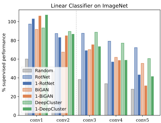
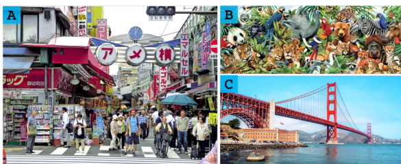
Figure 1: Single-image self-supervision. We show that several self-supervision methods can be used to train the first few layers of a deep neural networks using a single training image, such as this Image A, B or even C (above), provided that sufficient data augmentation is used.
图 1: 单图像自监督。我们证明了几种自监督方法可用于使用单张训练图像(如图像A、B甚至上方的C)训练深度神经网络的前几层,前提是使用足够的数据增强。
Our second finding is about the deeper layers of the network. For these, self-supervision remains inferior to strong supervision even if millions of images are used for training. Our finding is that this is unlikely to change with the addition of more data. In particular, we show that training these layers with self-supervision and a single image already achieves as much as two thirds of the performance that can be achieved by using a million different images.
我们的第二个发现与网络的深层结构有关。对于这些层,即便使用数百万张图像进行训练,自监督学习仍然弱于强监督学习。我们发现,增加更多数据也不太可能改变这一情况。具体而言,我们证明用自监督学习和单张图像训练这些层,已经能达到使用百万张不同图像训练所实现性能的三分之二。
We show that these conclusions hold true for three different self-supervised methods, BiGAN (Donahue et al., 2017), RotNet (Gidaris et al., 2018) and Deep Cluster (Caron et al., 2018), which are representative of the spectrum of techniques that are currently popular. We find that performance as a function of the amount of data is dependent on the method, but all three methods can indeed leverage a single image to learn the first few layers of a deep network almost “perfectly”.
我们证明这些结论适用于三种不同的自监督方法:BiGAN (Donahue et al., 2017)、RotNet (Gidaris et al., 2018) 和 Deep Cluster (Caron et al., 2018),它们代表了当前流行的技术谱系。我们发现性能随数据量的变化因方法而异,但这三种方法确实都能利用单张图像近乎"完美"地学习深度网络的前几层。
Overall, while our results do not improve self-supervision per-se, they help to characterize the limitations of current methods and to better focus on the important open challenges.
总体而言,虽然我们的结果并未直接提升自监督学习本身,但有助于揭示现有方法的局限性,并更聚焦于亟待解决的关键开放性问题。
2 RELATED WORK
2 相关工作
Our paper relates to three broad areas of research: (a) self-supervised/unsupervised learning, (b) learning from a single sample, and (c) designing/learning low-level feature extractors. We discuss closely related work for each.
我们的论文涉及三个广泛的研究领域:(a) 自监督/无监督学习,(b) 单样本学习,(c) 设计/学习低级特征提取器。我们将分别讨论密切相关的工作。
Self-supervised learning: A wide variety of proxy tasks, requiring no manual annotations, have been proposed for the self-training of deep convolutional neural networks. These methods use various cues and tasks namely, in-painting (Pathak et al., 2016), patch context and jigsaw puzzles (Doersch et al., 2015; Noroozi & Favaro, 2016; Noroozi et al., 2018; Mundhenk et al., 2017), clustering (Caron et al., 2018), noise-as-targets (Bojanowski & Joulin, 2017), color iz ation (Zhang et al., 2016; Larsson et al., 2017), generation (Jenni & Favaro, 2018; Ren & Lee, 2018; Donahue et al., 2017), geometry (Do sov it ski y et al., 2016; Gidaris et al., 2018) and counting (Noroozi et al., 2017). The idea is that the pretext task can be constructed automatically and easily on images alone. Thus, methods often modify information in the images and require the network to recover them. Inpainting or color iz ation techniques fall in this category. However these methods have the downside that the features are learned on modified images which potentially harms the generalization to unmodified ones. For example, color iz ation uses a gray scale image as input, thus the network cannot learn to extract color information, which can be important for other tasks.
自监督学习:研究者们提出了多种无需人工标注的代理任务,用于深度卷积神经网络的自我训练。这些方法利用不同线索和任务,包括图像修复 (Pathak et al., 2016)、局部上下文与拼图 (Doersch et al., 2015; Noroozi & Favaro, 2016; Noroozi et al., 2018; Mundhenk et al., 2017)、聚类 (Caron et al., 2018)、噪声作为目标 (Bojanowski & Joulin, 2017)、着色 (Zhang et al., 2016; Larsson et al., 2017)、生成 (Jenni & Favaro, 2018; Ren & Lee, 2018; Donahue et al., 2017)、几何 (Dosovitskiy et al., 2016; Gidaris et al., 2018) 以及计数 (Noroozi et al., 2017)。其核心思想是仅需图像即可自动构建预训练任务。因此,这些方法通常会对图像信息进行修改,并要求网络恢复原始信息。图像修复或着色技术便属于此类。然而这些方法的缺陷在于特征是从修改后的图像中学习的,可能影响对原始图像的泛化能力。例如着色任务使用灰度图像作为输入,导致网络无法学习提取色彩信息——这对其他任务可能至关重要。
Slightly less related are methods that use additional information to learn features. Here, often temporal information is used in the form of videos. Typical pretext tasks are based on temporalcontext (Misra et al., 2016; Wei et al., 2018; Lee et al., 2017; Sermanet et al., 2018), spatio-temporal cues (Isola et al., 2015; Gao et al., 2016; Wang et al., 2017), foreground-background segmentation via video segmentation (Pathak et al., 2017), optical-flow (Gan et al., 2018; Mahendran et al., 2018), future-frame synthesis (Srivastava et al., 2015), audio prediction from video (de Sa, 1994; Owens et al., 2016), audio-video alignment (Ar and j elo vic & Zisserman, 2017), ego-motion estimation (Jayaraman & Grauman, 2015), slow feature analysis with higher order temporal coherence (Jayaraman & Grauman, 2016), transformation between frames (Agrawal et al., 2015) and patch tracking in videos (Wang & Gupta, 2015). Since we are interested in learning features from as little data as one image, we cannot make use of methods that rely on video input.
相关性稍弱的是利用额外信息学习特征的方法。这类方法通常以视频形式使用时序信息,典型的预训练任务包括:时序上下文 (Misra et al., 2016; Wei et al., 2018; Lee et al., 2017; Sermanet et al., 2018) 、时空线索 (Isola et al., 2015; Gao et al., 2016; Wang et al., 2017) 、基于视频分割的前景-背景分离 (Pathak et al., 2017) 、光流 (Gan et al., 2018; Mahendran et al., 2018) 、未来帧合成 (Srivastava et al., 2015) 、视频音频预测 (de Sa, 1994; Owens et al., 2016) 、音视频对齐 (Ar and j elo vic & Zisserman, 2017) 、自我运动估计 (Jayaraman & Grauman, 2015) 、高阶时序一致性的慢特征分析 (Jayaraman & Grauman, 2016) 、帧间变换 (Agrawal et al., 2015) 以及视频中的区块追踪 (Wang & Gupta, 2015) 。由于我们的目标是从单张图像中学习特征,因此无法使用依赖视频输入的方法。
Our contribution inspects three unsupervised feature learning methods that use very different means of extracting information from the data: BiGAN (Donahue et al., 2017) utilizes a generative adversarial task, RotNet (Gidaris et al., 2018) exploits the photographic bias in the dataset and DeepCluster (Caron et al., 2018) learns stable feature representations under a number of image transformations by proxy labels obtained from clustering. These are described in more detail in the Methods section.
我们的贡献在于检验了三种无监督特征学习方法,它们采用截然不同的方式从数据中提取信息:BiGAN (Donahue et al., 2017) 利用生成对抗任务,RotNet (Gidaris et al., 2018) 利用数据集中的摄影偏差,而 DeepCluster (Caron et al., 2018) 通过聚类获得的代理标签,在多种图像变换下学习稳定的特征表示。这些方法在方法部分有更详细的描述。
Learning from a single sample: In some applications of computer vision, the bold idea of learning from a single sample comes out of necessity. For general object tracking, methods such as max margin correlation filters (Rodriguez et al., 2013) learn robust tracking templates from a single sample of the patch. A single image can also be used to learn and interpolate multi-scale textures with a GAN framework (Rott Shaham et al., 2019). Single sample learning was pursued by the semi-parametric exemplar SVM model (Mali sie wi cz et al., 2011). They learn one SVM per positive sample separating it from all negative patches mined from the background. While only one sample is used for the positive set, the negative set consists of thousands of images and is a necessary component of their method. The negative space was approximated by a multi-dimensional Gaussian by the Exemplar LDA (Hariharan et al., 2012). These SVMs, one per positive sample, are pooled together using a max aggregation. We differ from both of these approaches in that we do not use a large collection of negative images to train our model. Instead we restrict ourselves to a single or a few images with a systematic augmentation strategy.
从单一样本学习:在计算机视觉的某些应用中,从单一样本学习的大胆构想源于实际需求。通用目标追踪领域采用最大间隔相关滤波器(Rodriguez等人,2013)等方法,可从单一样本块中学习鲁棒的追踪模板。单个图像也可通过GAN框架(Rott Shaham等人,2019)实现多尺度纹理的学习与插值。半参数化样本SVM模型(Malisiewicz等人,2011)率先探索了单样本学习,该方法为每个正样本训练一个SVM,将其与从背景挖掘的所有负样本块分离。虽然正样本集仅使用一个样本,但负样本集由数千张图像组成,这是其方法的必要组成部分。Exemplar LDA(Hariharan等人,2012)通过多维高斯分布近似负空间。这些针对每个正样本训练的SVM通过最大聚合进行整合。我们的方法与上述两者不同:既不使用大量负样本图像训练模型,而是通过系统性数据增强策略,仅使用单张或少量图像进行学习。
Classical learned and hand-crafted low-level feature extractors: Learning and hand-crafting features pre-dates modern deep learning approaches and self-supervision techniques. For example the classical work of (Olshausen & Field, 1997) shows that edge-like filters can be learned via sparse coding of just 10 natural scene images. SIFT (Lowe, 2004) and HOG (Dalal & Triggs, 2005) have been used extensively before the advent of convolutional neural networks and, in many ways, they resemble the first layers of these networks. The scatter transform of Bruna & Mallat (2013); Oyallon et al. (2017) is an handcrafted design that aims at replacing at least the first few layers of a deep network. While these results show that effective low-level features can be handcrafted, this is insufficient to clarify the power and limitation of self-supervision in deep networks. For instance, it is not obvious whether deep networks can learn better low level features than these, how many images may be required to learn them, and how effective self-supervision may be in doing so. For instance, as we also show in the experiments, replacing low-level layers in a convolutional networks with handcrafted features such as Oyallon et al. (2017) may still decrease the overall performance of the model. Furthermore, this says little about deeper layers, which we also investigate.
经典学习和手工设计的低级特征提取器:学习和手工设计特征的方法早于现代深度学习方法和自监督技术。例如,(Olshausen & Field, 1997) 的经典研究表明,仅需10张自然场景图像即可通过稀疏编码学习到类似边缘的滤波器。在卷积神经网络出现之前,SIFT (Lowe, 2004) 和 HOG (Dalal & Triggs, 2005) 被广泛使用,并且在许多方面类似于这些网络的初始层。Bruna & Mallat (2013) 和 Oyallon et al. (2017) 提出的散射变换是一种手工设计,旨在替代深度网络的前几层。虽然这些结果表明有效的低级特征可以通过手工设计获得,但这不足以阐明自监督在深度网络中的能力和局限性。例如,尚不清楚深度网络是否能学习到比这些更好的低级特征、需要多少图像才能学习到这些特征,以及自监督在此过程中的效果如何。例如,正如我们在实验中也展示的那样,用手工设计的特征(如 Oyallon et al. (2017))替换卷积网络中的低级层仍可能降低模型的整体性能。此外,这并未涉及更深层的表现,我们对此也进行了研究。
In this work we show that current deep learning methods learn slightly better low-level representations than hand crafted features such as the scattering transform. Additionally, these representations can be learned from one single image with augmentations and without supervision. The results show how current self-supervised learning approaches that use one million images yield only relatively small gains when compared to what can be achieved from one image and augmentations, and motivates a renewed focus on augmentations and incorporating prior knowledge into feature extractors.
在本研究中,我们证明当前深度学习方法学习到的低层次表征略优于手工设计特征(如散射变换)。此外,这些表征可以通过数据增强从单张图像中无监督学习获得。结果表明:与单张图像增强方案相比,当前使用百万级图像的自我监督学习方法仅能带来相对有限的性能提升,这促使我们重新关注数据增强技术,并将先验知识融入特征提取器。
3 METHODS
3 方法
We discuss first our data and data augmentation strategy (section 3.1) and then we summarize the three different methods for unsupervised feature learning used in the experiments (section 3.2).
我们首先讨论数据及数据增强策略(见3.1节),随后总结实验中使用的三种无监督特征学习方法(见3.2节)。
3.1 DATA
3.1 数据
Our goal is to understand the performance of representation learning methods as a function of the image data used to train them. To make comparisons as fair as possible, we develop a protocol where only the nature of the training data is changed, but all other parameters remain fixed.
我们的目标是理解表征学习方法(representation learning)的性能与训练所用图像数据之间的关系。为确保比较的公平性,我们制定了实验方案:仅改变训练数据的性质,其他所有参数保持不变。
In order to do so, given a baseline method trained on $d$ source images, we replace those with another set of $d$ images. Of these, now only $N{\ll}d$ are source images (i.e. i.i.d. samples), while the remaining $d-N$ are augmentations of the source ones. Thus, the amount of information in the training data is controlled by $N$ and we can generate a continuum of datasets that vary from one extreme, utilizing a single source image $N=1$ , to the other extreme, using all $N{=}d$ original training set images. For example, if the baseline method is trained on ImageNet, then $d=1,281,167$ . When $N{=}1$ , it means that we train the method using a single source image and generate the remaining 1,281,166 images via augmentation. Other baselines use CIFAR-10/100 images, so in those cases $d=50\small{,}000$ instead.
为此,给定一个基于 $d$ 张源图像训练的基线方法,我们将其替换为另一组 $d$ 张图像。其中,现在仅有 $N{\ll}d$ 张是源图像(即独立同分布样本),而剩余的 $d-N$ 张是源图像的增强版本。因此,训练数据中的信息量由 $N$ 控制,我们可以生成一系列连续的数据集,其范围从一个极端(仅使用单张源图像 $N=1$)到另一个极端(使用全部 $N{=}d$ 张原始训练集图像)。例如,如果基线方法基于 ImageNet 训练,则 $d=1,281,167$。当 $N{=}1$ 时,意味着我们仅用一张源图像训练该方法,并通过增强生成剩余的 1,281,166 张图像。其他基线使用 CIFAR-10/100 图像,此时 $d=50\small{,}000$。
The data augmentation protocol, is an extreme version of augmentations already employed by most deep learning protocols. Each method we test, in fact, already performs some data augmentation internally. Thus, when the method is applied on our augmented data, this can be equivalently thought of as increment ing these “native” augmentations by concatenating them with our own.
数据增强协议是大多数深度学习协议已采用增强方法的极端版本。事实上,我们测试的每种方法内部都已执行了某种数据增强。因此,当方法应用于我们的增强数据时,可以等效地视为通过将"原生"增强与我们自身的增强相连接来增量提升这些增强效果。
Choice of augmentations. Next, we describe how the $N$ source images are expanded to additional $d{-N}$ images so that the models can be trained on exactly $d$ images, independent from the choice of $N$ . The idea is to use an aggressive form of data augmentation involving cropping, scaling, rotation, contrast changes, and adding noise. These transformations are representative of in variances that one may wish to incorporate in the features. Augmentation can be seen as imposing a prior on how we expect the manifold of natural images to look like. When training with very few images, these priors become more important since the model cannot extract them directly from data.
增强方式的选择。接下来,我们将描述如何将 $N$ 张源图像扩展到额外的 $d{-N}$ 张图像,从而确保无论 $N$ 的选择如何,模型都能在恰好 $d$ 张图像上进行训练。其核心思想是采用一种激进的数据增强方式,包括裁剪、缩放、旋转、对比度调整以及添加噪声。这些变换代表了人们可能希望融入特征中的不变性。增强可视为对我们期望自然图像流形形态的一种先验约束。当使用极少量图像进行训练时,这些先验变得尤为重要,因为模型无法直接从数据中提取它们。
Given a source image of size size $H\times W$ , we first extract a certain number of random patches of size $(w,h)$ , where $w\leq W$ and $h\leq H$ satisfy the additional constraints $\beta\le\frac{w h}{W H}$ and $\begin{array}{r}{\gamma^{\underline{{\mathbf{\Lambda}}}}\le\frac{h}{w}\le\gamma^{-1}}\end{array}$ . Thus, the smallest size of the crops is limited to be at least $\beta W H$ and at most the whole image. Additionally, changes to the aspect ratio are limited by $\gamma$ . In practice we use $\beta=10^{-3}$ and $\gamma={\textstyle\frac{3}{4}}$ .
给定一个尺寸为 $H\times W$ 的源图像,我们首先提取若干尺寸为 $(w,h)$ 的随机图像块,其中 $w\leq W$ 和 $h\leq H$ 需满足额外约束条件 $\beta\le\frac{w h}{W H}$ 以及 $\begin{array}{r}{\gamma^{\underline{{\mathbf{\Lambda}}}}\le\frac{h}{w}\le\gamma^{-1}}\end{array}$。因此,裁剪的最小尺寸被限制为至少 $\beta W H$,最大不超过整幅图像。此外,宽高比的变化受 $\gamma$ 限制。实际应用中我们采用 $\beta=10^{-3}$ 和 $\gamma={\textstyle\frac{3}{4}}$。
Second, good features should not change much by small image rotations, so images are rotated (before cropping to avoid border artifacts) by $\alpha\in(-35,35)$ degrees. Due to symmetry in image statistics, images are also flipped left-to-right with $50%$ probability.
其次,良好的特征应不会因小幅图像旋转而发生太大变化,因此图像会在裁剪前旋转(以避免边界伪影)$\alpha\in(-35,35)$度。由于图像统计的对称性,图像还会以$50%$的概率进行左右翻转。
Illumination changes are common in natural images, we thus expect image features to be robust to color and contrast changes. Thus, we employ a set of linear transformations in RGB space to model this variability in real data. Additionally, the color/intensity of single pixels should not affect the feature representation, as this does not change the contents of the image. To this end, color jitter with additive brightness, contrast and saturation are sampled from three uniform distributions in (0.6, 1.4) and hue noise from $\left(-0.1,0.1\right)$ is applied to the image patches. Finally, the cropped and transformed patches are scaled to the color range $(-1,1)$ and then rescaled to full $S\times S$ resolution to be supplied to each representation learning method, using bilinear interpolation. This formulation ensures that the patches are created in the target resolution $S$ , independent from the size and aspect ratio $W,H$ of the source image.
自然图像中光照变化十分常见,因此我们期望图像特征对色彩和对比度变化具有鲁棒性。为此,我们在RGB色彩空间中采用一组线性变换来模拟真实数据中的这种变化。此外,单个像素的颜色/强度不应影响特征表示,因为这不会改变图像内容。基于此,我们从(0.6, 1.4)区间内三个均匀分布中采样加性亮度、对比度和饱和度的色彩抖动,并对图像块施加$\left(-0.1,0.1\right)$范围的色调噪声。最后,裁剪变换后的图像块被缩放到$(-1,1)$色彩范围,再通过双线性插值重新缩放至$S\times S$目标分辨率,以供各表征学习方法使用。这种处理方式确保生成的图像块始终符合目标分辨率$S$,不受源图像尺寸$W,H$和宽高比的影响。
Real samples. The images used for the $N{=}1$ and $N{=}10$ experiments are shown in Figure 1 and the appendix respectively (this is all the training data used in such experiments). For the special case of using a single training image, i.e. $N{=}1$ , we have chosen one photographic $(2560\times1920)$ ) and one drawn image $(600\times225)$ , which we call Image A and Image $B$ , respectively. The two images were manually selected as they contain rich texture and are diverse, but their choice was not optimized for performance. We test only two images due to the cost of running a full set of experiments (each image is expanded up to $1.2\mathbf{M}$ times for training some of the models, as explained above). However, this is sufficient to prove our main points. We also test another $(1165\times585)$ Image $C$ to ablate the “crowded ness” of an image, as this latter contains large areas covering no objects. While resolution matters to some extent as a bigger image contains more pixels, the information within is still far more correlated, and thus more redundant than sampling several smaller images. In particular, the resolution difference in Image $\mathtt{A}$ and B appears to be negligible in our experiments. For CIFAR-10, where $S=32$ we only use Image B due to the resolution difference. In direct comparison, Image B is the size of about 132 CIFAR images which is still much less than $d=50\small{,}000$ . For $N>1$ , we select the source images randomly from each method’s training set.
真实样本。用于$N{=}1$和$N{=}10$实验的图像分别展示在图1和附录中(这些是此类实验使用的全部训练数据)。对于仅使用单张训练图像的特殊情况(即$N{=}1$),我们选择了一张摄影图像$(2560\times1920$)和一张手绘图像$(600\times225)$,分别称为图像A和图像$B$。这两张图像因其包含丰富纹理且具有多样性而被人工选取,但选择时未针对性能进行优化。由于完整实验的运行成本较高(如上所述,某些模型训练时单张图像需扩展至$1.2\mathbf{M}$倍),我们仅测试了两张图像。但这足以证明我们的主要观点。我们还测试了另一张$(1165\times585)$的图像$C$以分析图像的"拥挤度",因其包含大面积无物体区域。虽然分辨率在某种程度上会影响结果(更大图像包含更多像素),但其中的信息仍具有高度相关性,因此比采样多张小图像更具冗余性。具体而言,图像$\mathtt{A}$与B的分辨率差异在我们的实验中可忽略不计。对于$S=32$的CIFAR-10数据集,由于分辨率差异仅使用图像B。直接对比下,图像B的尺寸约为132张CIFAR图像,仍远小于$d=50\small{,}000$。当$N>1$时,我们从各方法的训练集中随机选取源图像。
3.2 REPRESENTATION LEARNING METHODS
3.2 表征学习方法
Generative models. Generative Adversarial Networks (GANs) (Goodfellow et al., 2014) learn to generate images using an adversarial objective: a generator network maps noise samples to image samples, approximating a target image distribution and a disc rim in at or network is tasked with dist ingui shing generated and real samples. Generator and disc rim in at or are pitched one against the other and learned together; when an equilibrium is reached, the generator produces images indistinguishable (at least from the viewpoint of the disc rim in at or) from real ones.
生成式模型。生成对抗网络 (GANs) (Goodfellow et al., 2014) 通过对抗目标学习生成图像:生成器网络将噪声样本映射为图像样本以逼近目标图像分布,而判别器网络负责区分生成样本与真实样本。生成器和判别器相互对抗并共同学习;当达到平衡时,生成器产生的图像将(至少从判别器视角)与真实图像无法区分。
Bidirectional Generative Adversarial Networks (BiGAN) (Donahue et al., 2017; Dumoulin et al., 2016) are an extension of GANs designed to learn a useful image representation as an approximate inverse of the generator through joint inference on an encoding and the image. This method’s native augmentation uses random crops and random horizontal flips to learn features from $S=128$ sized images. As opposed to the other two methods discussed below it employs leaky ReLU nonlinear i ties as is typical in GAN disc rim in at or s.
双向生成对抗网络(BiGAN) (Donahue et al., 2017; Dumoulin et al., 2016)是GAN的扩展,旨在通过对编码和图像的联合推断,学习生成器的近似逆映射来获得有用的图像表示。该方法采用随机裁剪和水平翻转作为原生数据增强策略,从$S=128$尺寸的图像中学习特征。与下文讨论的另外两种方法不同,它采用了GAN判别器中典型的leaky ReLU非线性激活函数。
Rotation. Most image datasets contain pictures that are ‘upright’ as this is how humans prefer to take and look at them. This photographer bias can be understood as a form of implicit data labelling. RotNet (Gidaris et al., 2018) exploits this by tasking a network with predicting the upright direction of a picture after applying to it a random rotation multiple of 90 degrees (in practice this is formulated as a 4-way classification problem). The authors reason that the concept of ‘upright’ requires learning high level concepts in the image and hence this method is not vulnerable to exploiting low-level visual information, encouraging the network to learn more abstract features. In our experiments, we test this hypothesis by learning from impoverished datasets that may lack the photographer bias. The native augmentations that RotNet uses on the $S=256$ inputs only comprise horizontal flips and non-scaled random crops to $224\times224$ .
旋转。大多数图像数据集包含"直立"的图片,因为这是人类喜欢拍摄和观看的方式。这种摄影师偏好可视为一种隐式数据标注形式。RotNet (Gidaris et al., 2018) 利用这一点,要求网络在图片随机旋转90度的倍数后预测其直立方向(实践中被表述为一个4分类问题)。作者认为"直立"概念需要学习图像中的高级概念,因此该方法不易受低级视觉信息干扰,能促使网络学习更抽象的特征。在我们的实验中,我们通过从可能缺乏摄影师偏见的贫乏数据集中学习来验证这一假设。RotNet在$S=256$输入上使用的原生增强仅包含水平翻转和缩放到$224\times224$的随机裁剪。
Clustering. Deep Cluster (Caron et al., 2018) is a recent state-of-the-art unsupervised representation learning method. This approach alternates $k$ -means clustering to produce pseudo-labels for the data and feature learning to fit the representation to these labels. The authors attribute the success of the method to the prior knowledge ingrained in the structure of the convolutional neural network (Ulyanov et al., 2018).
聚类。Deep Cluster (Caron et al., 2018) 是近期最先进的非监督表征学习方法。该方法交替使用 $k$ 均值聚类为数据生成伪标签,并通过特征学习使表征适配这些标签。作者将该方法的成功归因于卷积神经网络 (Ulyanov et al., 2018) 结构中固有的先验知识。
The method alternatives between a clustering step, in which $k$ -means is applied on the PCA-reduced features with $k=10^{4}$ , and a learning step, in which the network is trained to predict the cluster ID for each image under a set of augmentations (random resized crops with $\beta{\overset{\star}{=}}0.08,\gamma={\frac{3}{4}}$ and horizontal flips) that constitute its native augmentations used on top of the $S=256$ input images.
该方法交替进行聚类步骤和学习步骤。在聚类步骤中,对经过PCA降维的特征应用k均值聚类(k=10^4);在学习步骤中,网络通过一组增强操作(随机调整大小裁剪,其中β=0.08,γ=3/4,以及水平翻转)进行训练,以预测每张图像的聚类ID。这些增强操作是在S=256输入图像基础上应用的原生增强方法。
4 EXPERIMENTS
4 实验
We evaluate the representation learning methods on ImageNet and CIFAR-10/100 using linear probes (Section 4.1). After ablating various choices of transformations in our augmentation protocol (Section 4.2), we move to the core question of the paper: whether a large dataset is beneficial to unsupervised learning, especially for learning early convolutional features (Section 4.3).
我们在ImageNet和CIFAR-10/100数据集上使用线性探针(linear probe)评估表征学习方法(第4.1节)。通过消融研究分析数据增强方案中不同变换选择的影响(第4.2节)后,我们转向本文的核心问题:大规模数据集是否有利于无监督学习,特别是对早期卷积特征的学习(第4.3节)。
4.1 LINEAR PROBES AND BASELINE ARCHITECTURE
4.1 线性探针与基线架构
In order to quantify if a neural network has learned useful feature representations, we follow the standard approach of using linear probes (Zhang et al., 2017). This amounts to solving a difficult task such as ImageNet classification by training a linear classifier on top of pre-trained feature represent at ions, which are kept fixed. Linear class if i ers heavily rely on the quality of the representation since their disc rim i native power is low.
为了量化神经网络是否学到了有用的特征表示,我们遵循标准方法使用线性探针 [20]。该方法通过在预训练且保持固定的特征表示上训练线性分类器,来解决ImageNet分类等复杂任务。线性分类器高度依赖表示质量,因为其判别能力有限。
We apply linear probes to all intermediate convolutional layers of networks and train on the ImageNet LSVRC-12 (Deng et al., 2009) and CIFAR-10/100 (Krizhevsky, 2009) datasets, which are the standard benchmarks for evaluation in self-supervised learning. Our base encoder architecture is AlexNet (Krizhevsky et al., 2012) with BatchNorm, since this is a good representative model and is most often used in other unsupervised learning work for the purpose of benchmarking. This model has five convolutional blocks (each comprising a linear convolution later followed by ReLU and optionally max pooling). We insert the probes right after the ReLU layer in each block, and denote these entry points conv1 to conv5. Applying the linear probes at each convolutional layer allows studying the quality of the representation learned at different depths of the network.
我们对网络的所有中间卷积层应用线性探针,并在ImageNet LSVRC-12 (Deng et al., 2009) 和 CIFAR-10/100 (Krizhevsky, 2009) 数据集上进行训练,这些是自监督学习评估的标准基准。我们的基础编码器架构是带有BatchNorm的AlexNet (Krizhevsky et al., 2012),因为这是一个具有代表性的模型,并且最常用于其他无监督学习工作的基准测试。该模型包含五个卷积块(每个块由线性卷积层后接ReLU和可选的max pooling组成)。我们在每个块的ReLU层后立即插入探针,并将这些入口点标记为conv1至conv5。通过在每一卷积层应用线性探针,可以研究网络不同深度所学表示的质量。
Table 1: Ablating data augmentation using MonoGAN (left). Training a linear classifier on the features extracted at different depths of the network for CIFAR-10.
| CIFAR-10 | ||||
| conv1 | conv2 | conv3 | conv4 | |
| (a) Fully sup. | 66.5 | 70.1 | 72.4 | 75.9 |
| (b) Randomfeat. | 57.8 | 55.5 | 54.2 | 47.3 |
| (c) No aug. | 57.9 | 56.2 | 54.2 | 47.8 |
| (d) Jitter | 58.9 | 58.0 | 57.0 | 49.8 |
| (e) Rotation | 61.4 | 58.8 | 56.1 | 47.5 |
| (f) Scale | 67.9 | 69.3 | 67.9 | 59.1 |
| (g) Rot.& jitter | 64.9 | 63.6 | 61.0 | 53.4 |
| (h) Rot.&scale | 67.6 | 69.9 | 68.0 | 60.7 |
| (i) Jitter&scale | 68.1 | 71.3 | 69.5 | 62.4 |
| (G) All | 68.1 | 72.3 | 70.8 | 63.5 |
表 1: 使用 MonoGAN 进行数据增强消融实验 (左)。在 CIFAR-10 数据集上,针对网络不同深度提取的特征训练线性分类器的结果。
| CIFAR-10 | ||||
|---|---|---|---|---|
| conv1 | conv2 | conv3 | conv4 | |
| (a) 全监督 | 66.5 | 70.1 | 72.4 | 75.9 |
| (b) 随机特征 | 57.8 | 55.5 | 54.2 | 47.3 |
| (c) 无增强 | 57.9 | 56.2 | 54.2 | 47.8 |
| (d) 抖动 | 58.9 | 58.0 | 57.0 | 49.8 |
| (e) 旋转 | 61.4 | 58.8 | 56.1 | 47.5 |
| (f) 缩放 | 67.9 | 69.3 | 67.9 | 59.1 |
| (g) 旋转+抖动 | 64.9 | 63.6 | 61.0 | 53.4 |
| (h) 旋转+缩放 | 67.6 | 69.9 | 68.0 | 60.7 |
| (i) 抖动+缩放 | 68.1 | 71.3 | 69.5 | 62.4 |
| (G) 全部 | 68.1 | 72.3 | 70.8 | 63.5 |
Table 2: ImageNet LSVRC-12 linear probing evaluation (below). A linear classifier is trained on the (down sampled) activation s of each layer in the pretrained model. We report classification accuracy averaged over 10 crops. The ‡ indicated that numbers are taken from (Zhang et al., 2017).
| Method,Reference | ILSVRC-12 | ||||||
| #images | convl | conv2 | conv3 | conv4 | conv5 | ||
| (a) | Full-supervisiont | 1,281,167 | 19.3 | 36.3 | 44.2 | 48.3 | 50.5 |
| (b) | (Oyallon et al., 2017): Scattering | 0 | 18.9 | ||||
| (c) | Random* | 0 | 11.6 | 17.1 | 16.9 | 16.3 | 14.1 |
| (d) | (Krahenbuihl et al., 2016):k-meanst | 160 | 17.5 | 23.0 | 24.5 | 23.2 | 20.6 |
| (e) | (Donahue et al., 2017): BiGAN+ | 1,281,167 | 17.7 | 24.5 | 31.0 | 29.9 | 28.0 |
| (#) | mono,Image A | 1 | 20.4 | 30.9 | 33.4 | 28.4 | 16.0 |
| (g) | mono, Image B | 1 | 20.5 | 30.4 | 31.6 | 27.0 | 16.8 |
| (h) | deka | 10 | 16.2 | 16.5 | 16.5 | 13.1 | 7.5 |
| (i) | kilo | 1,000 | 16.1 | 17.7 | 18.3 | 17.6 | 13.5 |
| (! | (Gidaris et al., 2018): RotNet | 1,281,167 | 18.8 | 31.7 | 38.7 | 38.2 | 36.5 |
| (k) | mono, Image A | 1 | 19.9 | 30.2 | 30.6 | 27.6 | 21.9 |
| (1) | mono, Image B | 1 | 17.8 | 27.6 | 27.9 | 25.4 | 20.2 |
| (u) | deka | 10 | 19.6 | 30.7 | 32.6 | 28.9 | 22.6 |
| (n) | kilo | 1,000 | 21.0 | 33.5 | 36.5 | 34.0 | 29.4 |
| (0) | (Caron et al., 2018): DeepCluster | 1,281,167 | 18.0 | 32.5 | 39.2 | 37.2 | 30.6 |
| (d) | mono, Image A | 1 | 20.7 | 31.5 | 32.5 | 28.5 | 21.0 |
| (b) | mono, Image B | 1 | 19.7 | 30.1 | 31.6 | 28.5 | 20.4 |
| (r) | mono, Image C | 1 | 18.9 | 29.2 | 31.5 | 28.9 | 23.5 |
| (s) | deka | 10 | 18.5 | 29.0 | 31.1 | 28.2 | 21.9 |
| (t) | kilo | 1,000 | 19.5 | 29.8 | 33.0 | 31.7 | 26.8 |
表 2: ImageNet LSVRC-12 线性探测评估 (下)。在预训练模型的每一层 (降采样) 激活上训练线性分类器。报告结果为10次剪裁的平均分类准确率。‡ 表示数据来自 (Zhang et al., 2017)。
| 方法, 参考文献 | ILSVRC-12 | #images | conv1 | conv2 | conv3 | conv4 | conv5 |
|---|---|---|---|---|---|---|---|
| (a) Full-supervision | 1,281,167 | 19.3 | 36.3 | 44.2 | 48.3 | 50.5 | |
| (b) (Oyallon et al., 2017): Scattering | 0 | - | 18.9 | - | - | - | |
| (c) Random* | 0 | 11.6 | 17.1 | 16.9 | 16.3 | 14.1 | |
| (d) (Krahenbuihl et al., 2016): k-means | 160 | 17.5 | 23.0 | 24.5 | 23.2 | 20.6 | |
| (e) (Donahue et al., 2017): BiGAN+ | 1,281,167 | 17.7 | 24.5 | 31.0 | 29.9 | 28.0 | |
| (#) mono, Image A | 1 | 20.4 | 30.9 | 33.4 | 28.4 | 16.0 | |
| (g) mono, Image B | 1 | 20.5 | 30.4 | 31.6 | 27.0 | 16.8 | |
| (h) deka | 10 | 16.2 | 16.5 | 16.5 | 13.1 | 7.5 | |
| (i) kilo | 1,000 | 16.1 | 17.7 | 18.3 | 17.6 | 13.5 | |
| (!) (Gidaris et al., 2018): RotNet | 1,281,167 | 18.8 | 31.7 | 38.7 | 38.2 | 36.5 | |
| (k) mono, Image A | 1 | 19.9 | 30.2 | 30.6 | 27.6 | 21.9 | |
| (1) mono, Image B | 1 | 17.8 | 27.6 | 27.9 | 25.4 | 20.2 | |
| (u) deka | 10 | 19.6 | 30.7 | 32.6 | 28.9 | 22.6 | |
| (n) kilo | 1,000 | 21.0 | 33.5 | 36.5 | 34.0 | 29.4 | |
| (0) (Caron et al., 2018): DeepCluster | 1,281,167 | 18.0 | 32.5 | 39.2 | 37.2 | 30.6 | |
| (d) mono, Image A | 1 | 20.7 | 31.5 | 32.5 | 28.5 | 21.0 | |
| (b) mono, Image B | 1 | 19.7 | 30.1 | 31.6 | 28.5 | 20.4 | |
| (r) mono, Image C | 1 | 18.9 | 29.2 | 31.5 | 28.9 | 23.5 | |
| (s) deka | 10 | 18.5 | 29.0 | 31.1 | 28.2 | 21.9 | |
| (t) kilo | 1,000 | 19.5 | 29.8 | 33.0 | 31.7 | 26.8 |
Table 3: CIFAR-10/100. Accuracy of linear class if i ers on different network layers.
| Dataset | CIFAR-10 | CIFAR-100 | ||||||
| Model | conv1 | conv2 | conv3 | conv4 | conv1 | conv2 | conv3 | conv4 |
| Fully supervised | 66.5 | 70.1 | 72.4 | 75.9 | 38.7 | 43.6 | 44.4 | 46.5 |
| Random | 57.8 | 55.5 | 54.2 | 47.3 | 30.9 | 29.8 | 28.6 | 24.1 |
| RotNet | 64.4 | 65.6 | 65.6 | 59.1 | 36.0 | 35.9 | 34.2 | 25.8 |
| GAN (CIFAR-10) | 67.7 | 73.0 | 72.5 | 69.2 | 39.6 | 46.0 | 45.1 | 39.9 |
| GAN (CIFAR-100) | 一 | 一 | 38.1 | 42.2 | 44.0 | 46.6 | ||
| MonoGAN | 68.1 | 72.3 | 70.8 | 63.5 | 39.9 | 46.9 | 44.5 | 38.8 |
表 3: CIFAR-10/100. 不同网络层上线性分类器的准确率。
| 模型 | conv1 | conv2 | conv3 | conv4 | conv1 | conv2 | conv3 | conv4 |
|---|---|---|---|---|---|---|---|---|
| 数据集 | CIFAR-10 | CIFAR-100 | ||||||
| 全监督 | 66.5 | 70.1 | 72.4 | 75.9 | 38.7 | 43.6 | 44.4 | 46.5 |
| 随机初始化 | 57.8 | 55.5 | 54.2 | 47.3 | 30.9 | 29.8 | 28.6 | 24.1 |
| RotNet | 64.4 | 65.6 | 65.6 | 59.1 | 36.0 | 35.9 | 34.2 | 25.8 |
| GAN (CIFAR-10) | 67.7 | 73.0 | 72.5 | 69.2 | 39.6 | 46.0 | 45.1 | 39.9 |
| GAN (CIFAR-100) | - | - | - | - | 38.1 | 42.2 | 44.0 | 46.6 |
| MonoGAN | 68.1 | 72.3 | 70.8 | 63.5 | 39.9 | 46.9 | 44.5 | 38.8 |
Details. While linear probes are conceptually straightforward, there are several technical details that affect the final accuracy by a few percentage points. Unfortunately, prior work has used several slightly different setups, so that comparing results of different publications must be done with caution. To make matters more difficult, not all papers released evaluation source code. We prove this standardized testing code here2.
细节。虽然线性探针在概念上很简单,但有几个技术细节会影响最终准确率几个百分点。遗憾的是,先前工作使用了多种略有差异的设置,因此在比较不同论文结果时必须谨慎。更复杂的是,并非所有论文都公开了评估源代码。我们在此提供这套标准化测试代码2。
In our implementation, we follow the original proposal (Zhang et al., 2017) in pooling each represent ation to a vector with 9600, 9216, 9600, 9600, 9216 dimensions for $\mathtt{C O n v1}-5$ using adaptive max-pooling, and absorb the batch normalization weights into the preceding convolutions. For evaluation on ImageNet we follow RotNet to train linear probes: images are resized such that the shorter edge has a length of 256 pixels, random crops of $224\times224$ are computed and flipped horizontally with $50%$ probability. Learning lasts for 36 epochs and the learning rate schedule starts from 0.01 and is divided by five at epochs 5, 15 and 25. The top-1 accuracy of the linear classifier is then measured on the ImageNet validation subset. This uses Deep Cluster’s protocol, extracting 10 crops for each validation image (four at the corners and one at the center along with their horizontal flips) and averaging the prediction scores before the accuracy is computed. For CIFAR-10/100 data, we follow the same learning rate schedule and for both training and evaluation we do not reduce the dimensionality of the representations and keep the images’ original size of $32\times32$ .
在我们的实现中,我们遵循原始提案 (Zhang et al., 2017) 的方法,使用自适应最大池化将每个表示汇聚为维度分别为9600、9216、9600、9600、9216的向量(对应 $\mathtt{Conv1}-5$),并将批量归一化权重吸收到前序卷积中。对于ImageNet的评估,我们沿用RotNet的线性探针训练方法:将图像短边调整为256像素,随机裁剪 $224\times224$ 区域并以 $50%$ 概率进行水平翻转。训练持续36个周期,学习率从0.01开始,在第5、15和25周期时除以5。然后在ImageNet验证子集上测量线性分类器的top-1准确率。该流程采用Deep Cluster的协议,为每张验证图像提取10个裁剪区域(四个角部、一个中心及其水平翻转),在计算准确率前对预测分数取平均。对于CIFAR-10/100数据,我们采用相同学习率计划,在训练和评估时均不降低表示维度,并保持图像原始尺寸 $32\times32$。
4.2 EFFECT OF AUGMENTATIONS
4.2 数据增强的效果
In order to better understand which image transformations are important to learn a good feature representations, we analyze the impact of augmentation settings. For speed, these experiments are conducted using the CIFAR-10 images $d=50$ , 000 in the training set) and with the smaller source Image $\mathrm{B}$ and a GAN using the Wasser stein GAN formulation with gradient penalty (Gulrajani et al., 2017). The encoder is a smaller AlexNet-like CNN consisting of four convolutional layers (kernel sizes: $7,5,3,3$ ; strides: 3, 2, 2, 1) followed by a single fully connected layer as the disc rim in at or. Given that the GAN is trained on a single image (w/ augmentations), we call this setting MonoGAN.
为了更好地理解哪些图像变换对学习良好的特征表示至关重要,我们分析了数据增强设置的影响。出于速度考虑,这些实验使用CIFAR-10图像(训练集包含$d=50,000$张)以及较小的源图像$\mathrm{B}$,并采用带梯度惩罚的Wasserstein GAN框架(Gulrajani等人,2017)训练的GAN。编码器是一个较小的类AlexNet CNN,包含四个卷积层(核尺寸:$7,5,3,3$;步长:3, 2, 2, 1)和一个全连接层作为判别器。由于GAN是在单张图像(含增强)上训练的,我们将此设置称为MonoGAN。
Table 1 reports all $2^{3}$ combinations of the three main augmentations (scale, rotation, and jitter) and a randomly initialized network baseline (see Table 1 (b)) using the linear probes protocol discussed above. Without data augmentation the model only achieves marginally better performance than the random network (which also achieves a non-negligible level of performance (Ulyanov et al., 2017; Caron et al., 2018)). This is understandable since the dataset literally consists of a single training image cloned $d$ times. Color jitter and rotation slightly improve the performance of all probes by 1- $2%$ points, but random rescaling adds at least ten points at every depth (see Table 1 (f,h,i)) and is the most important single augmentation. A similar conclusion can be drawn when two augmentations are combined, although there are diminishing returns as more augmentations are combined. Overall, we find all three types of augmentations are of importance when training in the ultra-low data setting.
表1报告了三种主要数据增强方式(缩放、旋转和抖动)的所有$2^{3}$种组合,以及一个随机初始化网络基线(见表1(b))使用上述线性探针协议的结果。在没有数据增强的情况下,模型性能仅略优于随机网络(后者也达到了不可忽视的性能水平 (Ulyanov et al., 2017; Caron et al., 2018))。这是可以理解的,因为该数据集实际上只包含一张训练图像克隆$d$次。色彩抖动和旋转将所有探针的性能略微提高了1-$2%$个百分点,但随机缩放至少在每个深度增加了十个点(见表1(f,h,i)),是最重要的单一增强方式。当结合两种增强方式时,可以得出类似的结论,但随着更多增强方式的组合,收益会递减。总体而言,我们发现这三种增强方式在超低数据量训练中都很重要。
4.3 BENCHMARK EVALUATION
4.3 基准测试评估
We analyze how performance varies as a function $N$ , the number of actual samples that are used to generated the augmented datasets, and compare it to the gold-standard setup (in terms of choice of training data) defined in the papers that introduced each method. The evaluation is again based on linear probes (Section 4.1).
我们分析性能如何随函数$N$变化,$N$是用于生成增强数据集的实际样本数量,并将其与引入每种方法的论文中定义的黄金标准设置(在训练数据选择方面)进行比较。评估再次基于线性探针(第4.1节)。
Mono is enough. From Table 2 we make the following observations. Training with just a single source image (f,g,k,l,p,q) is much better than random initialization (c) for all layers. Notably, these models also outperform Gabor-like filters from Scattering networks (Bruna & Mallat, 2013), which are hand crafted image features, replacing the first two convolutional layers as in (Oyallon et al., 2017). Using the same protocol as in the paper, this only achieves an accuracy of $18.9%$ compared to (p)’s conv $2>30%$ .
单张图像足矣。从表2中我们得出以下观察结果:仅使用单张源图像(f,g,k,l,p,q)进行训练在所有层上都明显优于随机初始化(c)。值得注意的是,这些模型也优于散射网络(Bruna & Mallat, 2013)中的类Gabor滤波器(手工设计的图像特征),后者如(Oyallon et al., 2017)所述替换了前两个卷积层。采用与论文相同的实验方案,该方法仅能达到$18.9%$的准确率,而(p)的conv$2>30%$。
More importantly, when comparing within pretext task, even with one image we are able to improve the quality of conv1–conv3 features compared to full (unsupervised) ImageNet training for GAN based self-supervision (e-i). For the other methods $(\mathrm{j}-\mathrm{n},\mathrm{o}-\mathrm{s})$ we reach and also surpass the performance for the first layer and are within $1.5%$ points for the second. Given that the best unsupervised performance for conv2 is 32.5, our method using a single source Image A (Table 2, p) is remarkably close with 31.5.
更重要的是,在同一种预训练任务中进行比较时,即便仅使用单张图像,我们基于GAN的自监督方法(e-i)也能提升conv1-conv3特征的质量,优于完整的(无监督)ImageNet训练效果。对于其他方法$(\mathrm{j}-\mathrm{n},\mathrm{o}-\mathrm{s})$,我们在第一层达到并超越了其性能,第二层差距保持在$1.5%$以内。考虑到conv2的最佳无监督性能为32.5,我们仅使用单张源图像A的方法(表2, p)以31.5的成绩极为接近该水平。
Image contents. While we surpass the GAN based approach of (Donahue et al., 2017) for both single source images, we find more nuanced results for the other two methods: For RotNet, as expected, the photographic bias cannot be extracted from a single image. Thus its performance is low with little training data and increases together with the number of images (Table 2, j-n). When comparing Image $\mathtt{A}$ and B trained networks for RotNet, we find that the photograph yields better performance than the hand drawn animal image. This indicates that the method can extract rotation information from low level image features such as patches which is at first counter intuitive. Considering that the hand-drawn image does not work well, we can assume that lighting and shadows even in small patches can indeed give important cues on the up direction which can be learned even from a single (real) image. Deep Cluster shows poor performance in conv1 which we can improve upon in the single image setting (Table 2, o-r). Naturally, the image content matters: a trivial image without any image gradient (e.g. picture of a white wall) would not provide enough signal for any method. To better understand this issue, we also train Deep Cluster on the much less cluttered Image C to analyze how much the image influences our claims. We find that even though this image contains large parts of sky and sea, the performance is only slightly lower than that of Image A. This finding indicates that the augmentations can even compensate for large untextured areas and the exact choice of image is not critical.
图像内容。虽然在单源图像上我们超越了(Donahue et al., 2017)基于GAN的方法,但其他两种方法的结果更为微妙:对于RotNet,正如预期,无法从单张图像中提取摄影偏差。因此其性能在训练数据较少时表现不佳,并随着图像数量增加而提升(表2,j-n)。当比较使用图像$\mathtt{A}$和B训练的RotNet网络时,我们发现照片比手绘动物图像表现更好。这表明该方法可以从低层次图像特征(如图像块)中提取旋转信息,这起初是反直觉的。考虑到手绘图像效果不佳,我们可以假设即使是小块区域的光照和阴影也能提供关于上方方向的重要线索,这些线索甚至可以从单张(真实)图像中学习到。Deep Cluster在conv1层表现较差,但我们在单图像设置中改进了这一情况(表2,o-r)。自然,图像内容至关重要:没有任何图像梯度的平凡图像(例如白墙照片)无法为任何方法提供足够信号。为了更好地理解这个问题,我们还在更简洁的图像C上训练Deep Cluster,以分析图像对我们结论的影响程度。我们发现即使该图像包含大面积的天空和海洋,其性能仅略低于图像A。这一发现表明数据增强甚至可以补偿大面积无纹理区域,图像的具体选择并不关键。

Figure 2: conv1 filters trained using a single image. The 96 learned $(3\times11\times11)$ filters for the first layer of AlexNet are shown for each single training image and method along with their linear classifier performance. For visualization, each filter is normalized to be in the range of $(-1,1)$ .
图 2: 使用单张图像训练的conv1滤波器。展示了AlexNet第一层针对每张训练图像和方法学习的96个$(3\times11\times11)$滤波器及其线性分类器性能。为便于可视化,每个滤波器被归一化至$(-1,1)$范围。
More than one image. While BiGAN fails to converge for $N{\in}{10,1000}$ , most likely due to issues in learning from a distribution which is neither whole images nor only patches, we find that both RotNet and Deep Cluster improve their performance in deeper layers when increasing the number of training images. However, for conv1 and conv2, a single image is enough. In deeper layers, Deep Cluster seems to require large amounts of source images to yield the reported results as the deka- and kilo- variants start improving over the single image case (Table 2, o-t). This need for data also explains the gap between the two input images which have different resolutions. Summarizing Table 2, we can conclude that learning conv1, conv2 and for the most part conv3 (33.4 vs. 39.4) on over 1M images does not yield a significant performance increase over using one single training image — a highly unexpected result.
多图像情况。虽然BiGAN在$N{\in}{10,1000}$时未能收敛(很可能是由于学习对象既非完整图像也非局部图像块导致的分布学习问题),但我们发现RotNet和Deep Cluster在深层网络中会随着训练图像数量的增加而提升性能。不过对于conv1和conv2层而言,单张图像已足够。在更深层网络中,Deep Cluster似乎需要大量源图像才能达到文献报告的结果(表2中o-t列显示,十倍和千倍数据量变体开始优于单图像情况)。这种数据需求也解释了两种不同分辨率输入图像之间的性能差距。总结表2可知:在超过100万张图像上训练conv1、conv2及大部分conv3层(33.4 vs. 39.4)相比使用单张训练图像并未带来显著性能提升——这一结果极具颠覆性。
Generalization. In Table 3, we show the results of training linear class if i ers for the CIFAR-10 dataset and compare against various baselines. We find that the GAN trained on the smaller Image B outperforms all other methods including the fully-supervised trained one for the first convolutional layer. We also outperform the same architecture trained on the full CIFAR-10 training set using RotNet, which might be due to the fact that either CIFAR images do not contain much information about the orientation of the picture or because they do not contain as many objects as in ImageNet. While the GAN trained on the whole dataset outperforms the MonoGAN on the deeper layers, the gap stays very small until the last layer. These findings are also reflected in the experiments on the CIFAR-100 dataset shown in Table 3. We find that our method obtains the best performance for the first two layers, even against the fully supervised version. The gap between our mono variant and the other methods increases again with deeper layers, hinting to the fact that we cannot learn very high level concepts in deeper layers from just one single image. These results corroborate the finding that our method allows learning very general iz able early features that are not domain dependent.
泛化性。表3展示了在CIFAR-10数据集上训练线性分类器的结果,并与多种基线方法进行比较。我们发现,在较小Image B上训练的GAN(生成对抗网络)优于包括全监督训练方法在内的所有其他方法(针对第一卷积层)。我们还超越了使用RotNet在整个CIFAR-10训练集上训练的相同架构,这可能是因为CIFAR图像要么不包含太多关于图片方向的信息,要么其包含的对象数量不及ImageNet。虽然在完整数据集上训练的GAN在深层网络表现优于MonoGAN,但直到最后一层两者的差距仍然很小。这些发现在表3所示的CIFAR-100数据集实验中也得到印证。我们的方法在前两层获得了最佳性能,甚至优于全监督版本。随着网络层数加深,我们的单样本变体与其他方法的差距再次拉大,这表明我们无法仅从单张图像学习深层网络中的高级概念。这些结果证实了我们的方法能够学习与领域无关、可高度泛化的早期特征。
4.4 QUALITATIVE ANALYSIS
4.4 定性分析
Visual comparison of weights. In Figure 2, we compare the learned filters of all first-layer convolutions of an AlexNet trained with the different methods and a single image. First, we find that the filters closely resemble those obtained via supervised training: Gabor-like edge detectors and various color blobs. Second, we find that the look is not easily predictive of its performance, e.g.
权重可视化对比。在图2中,我们比较了使用不同方法和单张图像训练的AlexNet所有第一层卷积的学习滤波器。首先发现这些滤波器与监督训练获得的非常相似:类似Gabor的边缘检测器和各种色块。其次观察到滤波器外观难以预测其性能,例如
while generative ly learned filters (BiGAN) show many edge detectors, its linear probes performance is about the same as that of Deep Cluster which seems to learn many somewhat redundant point features. However, we also find that some edge detectors are required, as we can confirm from RotNet and Deep Cluster trained on Image B, which yield less crisp filters and worse performances.
虽然生成式学习滤波器(BiGAN)显示出许多边缘检测器,但其线性探针性能与Deep Cluster大致相当,后者似乎学习了许多略显冗余的点特征。然而,我们也发现某些边缘检测器是必要的——这一点可以通过在Image B上训练的RotNet和Deep Cluster得到验证,它们生成的滤波器清晰度较低且性能较差。
Table 4: Finetuning experiments The pretrained model’s first two convolutions are left frozen (or replaced by the Scattering transform) and the nework is retrained using ImageNet LSVRC-12 training set.
| Top-1 | |
| Full sup. | 59.4 |
| Random | 42.6 |
| Scattering | 49.2 |
| BiGAN,A | 51.4 |
| RotNet,A | 49.5 |
| DeepCluster A | 52.5 |
表 4: 微调实验
预训练模型的前两个卷积层保持冻结状态(或替换为散射变换),并使用ImageNet LSVRC-12训练集重新训练网络。
| Top-1 | |
|---|---|
| Full sup. | 59.4 |
| Random | 42.6 |
| Scattering | 49.2 |
| BiGAN,A | 51.4 |
| RotNet,A | 49.5 |
| DeepCluster A | 52.5 |

Figure 3: Style transfer with single-image pretraining. We show two style transfer results using the Image A trained BiGAN and the ImageNet pretrained AlexNet.
图 3: 单图像预训练的风格迁移。我们展示了使用图像A训练的BiGAN和ImageNet预训练的AlexNet的两种风格迁移结果。
Fine-tuning instead of freezing. In Tab. 4, we show the results of retraining a network with the first two convolutional filters, or the scattering transform from (Oyallon et al., 2017), left frozen. We observe that our single image trained Deep Cluster and BiGAN models achieve performances closes to the supervised benchmark. Notably, the scattering transform as a replacement for conv1-2 performs slightly worse than the analyzed single image methods. We also show in the appendix the results of retraining a network initialized with the first two convolutional layers obtained from a single image and subsequently linearly probing the model. The results are shown in Appendix Tab. 5 and we find that we can recover the performance of fully-supervised networks, i.e. the first two convolutional filters trained from just a single image generalize well and do not get stuck in an image specific minimum.
微调而非冻结。在表4中,我们展示了重新训练网络时保持前两个卷积滤波器或 (Oyallon et al., 2017) 提出的散射变换冻结的结果。我们观察到,使用单张图像训练的Deep Cluster和BiGAN模型性能接近监督学习的基准。值得注意的是,用散射变换替代conv1-2的表现略逊于所分析的单图方法。附录中还展示了使用单图初始化前两个卷积层后重新训练网络并进行线性探测的结果,详见附录表5。我们发现可以恢复全监督网络的性能,即仅用单张图像训练的前两个卷积滤波器具有良好泛化性,不会陷入图像特定的局部极小值。
Neural style transfer. Lastly, we show how our features trained on only a single image can be used for other applications. In Figure 3 we show two basic style transfers using the method of (Gatys et al., 2016) from an official PyTorch tutorial3. Image content and style are separated and the style is transferred from the source to target image using all CNN features, not just the shallow layers. We visually compare the results of using our features and from full ImageNet supervision. We find almost no visual differences in the stylized images and can conclude that our early features are equally powerful as fully supervised ones for this task.
神经风格迁移。最后,我们展示了仅用单张图像训练的特征如何应用于其他场景。在图 3 中,我们通过官方 PyTorch 教程3展示了基于 (Gatys et al., 2016) 方法的两种基础风格迁移效果。该方法分离了图像内容与风格,并利用所有 CNN 特征(不仅限于浅层)将源图像风格迁移至目标图像。我们直观对比了使用自训练特征与全监督 ImageNet 特征的效果,发现风格化图像几乎不存在视觉差异,由此得出结论:对于此类任务,我们的早期特征与全监督特征具有同等效力。
5 CONCLUSIONS
5 结论
We have made the surprising observation that we can learn good and general iz able features through self-supervision from one single source image, provided that sufficient data augmentation is used. Our results complement recent works (Mahajan et al., 2018; Goyal et al., 2019) that have investigated self-supervision in the very large data regime. Our main conclusion is that these methods succeed perfectly in capturing the simplest image statistics, but that for deeper layers a gap exist with strong supervision which is compensated only in limited manner by using large datasets. This novel finding motivates a renewed focus on the role of augmentations in self-supervised learning and critical rethinking of how to better leverage the available data.
我们意外地发现,通过单张源图像的自监督学习,配合充分的数据增强,就能习得优质且泛化性强的特征。这一结论与近期研究 (Mahajan et al., 2018; Goyal et al., 2019) 在大数据量下的自监督探索形成互补。核心发现表明:现有方法能完美捕捉最基础的图像统计特征,但在更深层网络仍存在与强监督学习的性能差距——仅靠扩大数据集只能有限弥补这一差距。该新发现促使我们重新审视数据增强在自监督学习中的作用,并亟需反思如何更高效利用现有数据。
ACKNOWLEDGEMENTS.
致谢
We thank Aravindh Mahendran for fruitful discussions. Yuki Asano gratefully acknowledges support from the EPSRC Centre for Doctoral Training in Autonomous Intelligent Machines & Systems (EP/L015897/1). The work is supported by ERC IDIU-638009.
我们感谢Aravindh Mahendran富有成效的讨论。Yuki Asano衷心感谢EPSRC自主智能机器与系统博士培训中心(EP/L015897/1)的支持。该工作由ERC IDIU-638009资助。
A APPENDIX
A 附录
A.1 IMAGENET TRAINING IMAGES
A.1 IMAGENET 训练图像

Figure 4: ImageNet images for the $N{=}10$ experiments.
图 4: ImageNet 图像在 $N{=}10$ 实验中的示例。
The images used for the $N{=}10$ experiments are shown in fig. 4.
用于 $N{=}10$ 次实验的图像如图 4 所示。
A.2 VISUAL COMPARISON OF FILTERS
A.2 滤波器视觉对比

Figure 5: Filter visualization. We show activation maximization (left) and retrieval of top 9 activated images from the training set of ImageNet (right) for four random non-cherry picked target filters. From top to bottom: conv1-5 of the BiGAN trained on a single image A. The filter visualization is obtained by learning a (regularized) input image that maximizes the response to the target filter using the library Lucid (Olah et al., 2018).
图 5: 滤波器可视化。我们展示了四个随机选取(未刻意筛选)的目标滤波器的激活最大化结果(左)及从ImageNet训练集中检索到的前9个激活图像(右)。从上至下: 在单张图像A上训练的BiGAN的conv1-5层滤波器。该可视化通过使用Lucid库(Olah等人, 2018)学习使目标滤波器响应最大化的(正则化)输入图像获得。
In order to understand what deeper neurons are responding to in our model, we visualize random neurons via activation maximization (Erhan et al., 2009; Zeiler & Fergus, 2014) in each layer. Additionally, we retrieve the top-9 images in the ImageNet training set that activate each neuron most in Figure 5. Since the mono networks are not trained on the ImageNet dataset, it can be used here for visualization. From the first convolutional layer we find typical neurons strongly reacting to oriented edges. In layers 2-4 we find patterns such as grids (conv2:3), and textures such as leopard skin (conv2:2) and round grid cover (conv4:4). Confirming our hypothesis that the neural network is only extracting patterns and not semantic information, we do not find any neurons particularly specialized to certain objects even in higher levels as for example dog faces or similar which can be fund in supervised networks. This finding aligns with the observations of other unsupervised methods (Caron et al., 2018; Zhang et al., 2017). As most neurons extract simple patterns and textures, the surprising effectiveness of training a network using a single image can be explained by the recent finding that even CNNs trained on ImageNet rely on texture (as opposed to shape) information to classify (Geirhos et al., 2019).
为了理解模型中深层神经元对何种特征产生响应,我们通过激活最大化(Erhan et al., 2009; Zeiler & Fergus, 2014)方法对各层随机神经元进行可视化。此外,在图5中我们提取了ImageNet训练集中最能激活每个神经元的前9张图像。由于单目网络未在ImageNet数据集上训练,该数据集可用于此处的可视化分析。在第一个卷积层中,我们发现典型神经元对定向边缘有强烈反应。在2-4层中,我们观察到网格(conv2:3)等模式,以及豹纹(conv2:2)和圆形网格覆盖物(conv4:4)等纹理特征。这验证了我们的假设:该神经网络仅提取模式特征而非语义信息,即使在更高层级也未发现专门针对特定物体(如监督网络中常见的狗脸等)的特化神经元。该发现与其他无监督方法的观测结果一致(Caron et al., 2018; Zhang et al., 2017)。由于多数神经元提取的是简单模式和纹理特征,使用单张图像训练网络仍能取得显著效果的原因在于:最新研究表明,即使在ImageNet上训练的CNN也主要依赖纹理(而非形状)信息进行分类(Geirhos et al., 2019)。
Table 5: Finetuning experiments Models are initialized using conv1 and conv2 from various single image trained models and the whole network is fine-tuned using ImageNet LSVRC-12 training set. Accuracy is averaged over 10 crops.
| c1 c2 c3 C4 |
| c5 19.3 36.3 4 44.2 48.3 50.5 |
| Full sup. |
| BiGAN,A 22.5 37.6 44.2 47.6 48.3 |
| RotNet,A 22.0 38.2 44.8 49.2 51.8 DeepCluster, A 21.8 35.9 43.6 48.8 50.4 |
表 5: 微调实验
模型使用来自不同单图像训练模型的conv1和conv2进行初始化,并使用ImageNet LSVRC-12训练集对整个网络进行微调。准确率为10次裁剪的平均值。
| c1 | c2 | c3 | C4 |
|---|---|---|---|
| c5 | 19.3 | 36.3 | 4 |
| Full sup. | |||
| BiGAN,A | 22.5 | 37.6 | 44.2 |
| RotNet,A | 22.0 | 38.2 | 44.8 |
| DeepCluster, A | 21.8 | 35.9 | 43.6 |
A.3 RETRAINING FROM SINGLE IMAGE INITIALIZATION
A.3 基于单张图像初始化的重新训练
In Table 5, we initialize AlexNet models using the first two convolutional filters learned from a single image and retrain them using ImageNet. We find that the networks recover their performance fully and the first filters do not make the network stuck in a bad local minimum despite having been trained on a single image from a different distribution. The difference from the BiGAN to the full supervision model is likely due to it using a smaller input resolution (112 instead of 224), as the BiGAN’s output resolution is limited.
在表5中,我们使用从单张图像学习到的前两个卷积滤波器初始化AlexNet模型,并用ImageNet重新训练。研究发现,尽管这些初始滤波器是在不同分布的单张图像上训练的,网络仍能完全恢复性能,且不会陷入不良局部极小值。与全监督模型的差异可能源于BiGAN使用了较低输入分辨率(112而非224),因为其输出分辨率受限。
A.4 LINEAR PROBES ON IMAGENET
A.4 在 ImageNet 上的线性探针
We show two plots of the ImageNet linear probes results (Table 2 of the paper) in fig. 6. On the left we plot performance per layer in absolute scale. Naturally the performance of the supervised model improves with depth, while all unsupervised models degrade after conv3. From the relative plot on the right, it becomes clear that with our training scheme, we can even slightly surpass supervised performance on conv1 presumably since our model is trained with sometimes very small patches, thus receiving an emphasis on learning good low level filters. The gap between all self-supervised methods and the supervised baseline increases with depth, due to the fact that the supervised model is trained for this specific task, whereas the self-supervised models learn from a surrogate task without labels.
我们在图6中展示了ImageNet线性探测结果(论文中的表2)的两幅图表。左侧以绝对尺度绘制了每层性能表现。监督模型性能随深度自然提升,而所有无监督模型在conv3后性能下降。从右侧的相对性能图可以明显看出,采用我们的训练方案后,甚至在conv1层能略微超越监督学习性能,这很可能是因为我们的模型有时使用极小图像块(patch)进行训练,从而强化了底层滤波器学习。随着网络深度增加,所有自监督方法与监督基线之间的差距逐渐扩大,这是由于监督模型针对特定任务训练,而自监督模型是从无标签的替代任务中学习。

Figure 6: Linear Class if i ers on ImageNet. Classification accuracies of linear class if i ers trained on the representations from Table 2 are shown in absolute scale.
图 6: ImageNet上的线性分类器。基于表2表示训练的线性分类器准确率以绝对值形式展示。
A.5 EXAMPLE AUGMENTED TRAINING DATA
A.5 增强训练数据示例
In figs. 7 to 10 we show example patches generated by our augmentation strategy for the datasets with different N. Even though the images and patches are very different in color and shape distribu
图 7 至图 10 展示了我们针对不同 N 值数据集所采用的增强策略生成的示例图像块。尽管这些图像和图像块在颜色与形状分布上存在显著差异
tion, our model learns weights that perform similarly in the linear probes benchmark (see Table 2 in the paper).
我们的模型学习到的权重在线性探测基准测试中表现相似(参见论文中的表2)。

Figure 7: Example crops of Image A ( $N=1$ ) dataset.
图 7: Image A ( $N=1$ ) 数据集的示例裁剪图。

Figure 8: Example crops of Image B $N=1$ ) dataset. 50 samples were selected randomly.
图 8: Image B $N=1$ 数据集的示例裁剪。随机选取了50个样本。

Figure 9: Example crops of deka $N=10$ ) dataset. 50 samples were selected randomly.
图 9: deka数据集 (N=10) 的示例裁剪。随机选取了50个样本。

Figure 10: Example crops of kilo ( $\overline{{N=1000}},$ ) dataset. 50 samples were selected randomly.
图 10: 千样本 ( $\overline{{N=1000}},$ ) 数据集示例裁剪。随机选取了50个样本。