Select, Label, and Mix: Learning Disc rim i native Invariant Feature Representations for Partial Domain Adaptation
选择、标注与混合:面向部分域适应的判别性不变特征表示学习
Abstract
摘要
Partial domain adaptation which assumes that the unknown target label space is a subset of the source label space has attracted much attention in computer vision. Despite recent progress, existing methods often suffer from three key problems: negative transfer, lack of disc rim in a bility, and domain invariance in the latent space. To alleviate the above issues, we develop a novel ‘Select, Label, and Mix’ (SLM) framework that aims to learn disc rim i native invariant feature representations for partial domain adaptation. First, we present an efficient “select” module that au- to mati call y filters out the outlier source samples to avoid negative transfer while aligning distributions across both domains. Second, the “label” module iterative ly trains the classifier using both the labeled source domain data and the generated pseudo-labels for the target domain to enhance the disc rim inability of the latent space. Finally, the “mix” module utilizes domain mixup regular iz ation jointly with the other two modules to explore more intrinsic structures across domains leading to a domain-invariant latent space for partial domain adaptation. Extensive experiments on several benchmark datasets for partial domain adaptation demonstrate the superiority of our proposed framework over state-of-the-art methods. Project page: https: //cvir.github.io/projects/slm.
部分域适应(Partial Domain Adaptation)假设未知目标标签空间是源标签空间的子集,这一领域在计算机视觉中备受关注。尽管已有进展,现有方法仍面临三个关键问题:负迁移(negative transfer)、潜在空间缺乏判别性(discriminability)以及域不变性不足。为缓解这些问题,我们提出了一种新颖的"选择-标注-混合"(Select, Label, and Mix, SLM)框架,旨在学习具有判别性的域不变特征表示。首先,"选择"模块通过自动过滤异常源样本避免负迁移,同时实现跨域分布对齐;其次,"标注"模块利用标注源数据和生成的目标域伪标签迭代训练分类器,增强潜在空间的判别性;最后,"混合"模块结合域混合(mixup)正则化与前两个模块,探索跨域本质结构,构建适用于部分域适应的域不变潜在空间。在多个基准数据集上的实验表明,该框架显著优于现有最优方法。项目页面:https://cvir.github.io/projects/slm。
1. Introduction
1. 引言
Deep neural networks usually have recently shown impressive performance on many visual tasks by leveraging large collections of labeled data. However, they usually do not generalize well to domains that are not distributed identically to the training data. Domain adaptation [10, 46] addresses this problem by transferring knowledge from a label-rich source domain to a target domain where labels are scarce or unavailable. However, standard domain adaptation algorithms often assume that the source and target domains share the same label space [11, 13, 25, 26, 27]. Since large-scale labelled datasets are readily accessible as source domain data, a more realistic scenario is partial domain adaptation (PDA), which assumes that target label space is a subset of source label space, that has received increasing research attention recently [2, 8, 9, 17].
深度神经网络近年来通过利用大量标注数据,在许多视觉任务上展现出令人印象深刻的性能。然而,它们通常无法很好地泛化到与训练数据分布不同的领域。领域自适应 (domain adaptation) [10, 46] 通过将知识从标签丰富的源领域迁移到标签稀缺或不可用的目标领域来解决这一问题。但标准领域自适应算法通常假设源领域和目标领域共享相同的标签空间 [11, 13, 25, 26, 27]。由于大规模标注数据集可作为源领域数据便捷获取,更现实的场景是部分领域自适应 (PDA) —— 该设定假设目标标签空间是源标签空间的子集,近年来该方向获得了越来越多的研究关注 [2, 8, 9, 17]。
Several methods have been proposed to solve partial domain adaptation by re weighting the source domain samples [2, 8, 9, 17, 50, 54]. However, (1) most of the existing methods still suffer from negative transfer due to presence of outlier source domain classes, which cripples domainwise transfer with un transferable knowledge; (2) in absence of the labels, they often neglect the class-aware information in target domain which fails to guarantee the disc rim in a bility of the latent space; and (3) given filtering of the outliers, limited number of samples from the source and target domain are not alone sufficient to learn domain invariant features for such a complex problem. As a result, a domain classifier may falsely align the unlabeled target samples with samples of a different class in the source domain, leading to inconsistent predictions.
为解决部分域适应问题,已有多种方法通过重新加权源域样本提出[2, 8, 9, 17, 50, 54]。然而,(1) 现有方法大多仍因异常源域类别的存在而遭受负迁移,导致无法传递的知识破坏了域间迁移;(2) 在缺乏标签的情况下,它们常忽略目标域中的类别感知信息,难以保证潜在空间的可判别性;(3) 即便过滤异常样本,仅靠源域和目标域有限的样本量仍不足以为此复杂问题学习域不变特征。这会导致域分类器可能错误地将未标记目标样本与源域中不同类别的样本对齐,从而产生不一致的预测。
To address these challenges, we propose a novel end-toend Select, Label, and Mix (SLM) framework for learning disc rim i native invariant features while preventing negative transfer in partial domain adaptation. Our framework consists of three unique modules working in concert, i.e., select, label and mix, as shown in Figure 1. First, the select module facilitates the identification of relevant source samples preventing the negative transfer. To be specific, our main idea is to learn a model (referred to as selector network) that outputs probabilities of binary decisions for selecting or discarding each source domain sample before aligning source and target distributions using an adversarial disc rim in at or [12]. As these decision functions are discrete and non-differentiable, we rely on Gumbel Softmax sampling [20] to learn the policy jointly with network parameters through standard back-propagation, without resorting to complex reinforcement learning settings, as in [8, 9]. Second, we develop an efficient self-labeling strategy that iterative ly trains the classifier using both labeled source domain data and generated soft pseudo-labels for target domain to enhance the disc rim in a bil ty of the latent space. Finally, the mix module utilizes both intra- and inter-domain mixup regular iz at ions [53] to generate convex combinations of pairs of training samples and their labels in both domains. The mix strategy not only helps to explore more intrinsic structures across domains leading to an invariant latent space, but also helps to stabilize the domain discriminator while bridging distribution shift across domains.
为解决这些挑战,我们提出了一种新颖的端到端选择、标注与混合(SLM)框架,用于学习判别性不变特征,同时避免部分域适应中的负迁移。如图1所示,该框架由三个协同工作的独特模块组成:选择、标注和混合。首先,选择模块通过识别相关源样本防止负迁移。具体而言,我们提出学习一个选择器网络(selector network),在采用对抗判别器[12]对齐源域与目标域分布前,该网络会输出每个源域样本的二元选择概率。由于这些决策函数是离散且不可微的,我们采用Gumbel Softmax采样[20]将策略学习与网络参数通过标准反向传播联合优化,避免了如[8,9]中复杂的强化学习设置。其次,我们开发了一种高效的自标注策略,通过迭代训练分类器同时使用带标注的源域数据和为目标域生成的软伪标签,以增强潜在空间的判别性。最后,混合模块利用域内与域间混合正则化[53],生成两域训练样本及其标签的凸组合。这种混合策略不仅能探索跨域更本质的结构从而构建不变潜在空间,还能在弥合域间分布偏移时稳定域判别器。

Figure 1: A conceptual overview of our approach. Our proposed approach adopts three unique modules namely Select, Label and Mix in a unified framework to mitigate domain shift and generalize the model to an unlabelled target domain with a label space which is a subset of that of the labelled source domain. Our Select module discards outlier samples from the source domain to eliminate negative transfer of un transferable knowledge. On the other hand, Label and Mix modules ensure disc rim inability and invariance of the latent space respectively while adapting the source classifier to the target domain in partial domain adaptation setting. Best viewed in color.
图 1: 方法概念概述。我们提出的方法在一个统一框架中采用三个独特模块——选择 (Select)、标注 (Label) 和混合 (Mix),以缓解域偏移并使模型能泛化至未标注目标域,其标签空间是已标注源域标签空间的子集。选择模块通过剔除源域中的异常样本来消除不可迁移知识的负迁移。另一方面,在部分域自适应设置中,标注模块和混合模块分别确保潜在空间的判别性和不变性,同时使源分类器适应目标域。建议彩色查看。
Our proposed modules are simple yet effective which explore three unique aspects for the first time in partial domain adaptation setting in an end-to-end manner. Specifically, in each mini-batch, our framework simultaneously eliminates negative transfer by removing outlier source samples and learns disc rim i native invariant features by labeling and mixing samples. Experiments on four datasets illustrate the effectiveness of our proposed framework in achieving new state-of-the-art performance for partial domain adaptation (e.g., our approach outperforms DRCN [22] by $\mathbf{18.9%}$ on the challenging VisDA-2017 [36] benchmark). To summarize, our key contributions include:
我们提出的模块简洁高效,首次在部分域自适应(partial domain adaptation)设置中以端到端(end-to-end)方式探索了三个独特维度。具体而言,在每个小批量(mini-batch)中,我们的框架通过剔除异常源样本消除负迁移(negative transfer),同时通过样本标注与混合学习判别性不变特征(discriminative invariant features)。在四个数据集上的实验表明,我们提出的框架在部分域自适应任务中实现了最先进的性能(例如在具有挑战性的VisDA-2017[36]基准测试中,我们的方法以$\mathbf{18.9%}$的优势超越DRCN[22])。核心贡献可归纳为:
• We propose a novel Select, Label, and Mix (SLM) framework for learning disc rim i native and invariant feature representation while preventing intrinsic negative transfer in partial domain adaptation. • We develop a simple and efficient source sample selection strategy where the selector network is jointly trained with the domain adaptation model using backpropagation through Gumbel Softmax sampling. • We conduct extensive experiments on four datasets, including Office31 [38], Office-Home [44], ImageNetCaltech, and VisDA-2017 [36] to demonstrate superiority of our approach over state-of-the-art methods.
• 我们提出了一种新颖的选择、标注与混合 (Select, Label, and Mix, SLM) 框架,用于在部分域适应中学习判别性和不变性特征表示,同时防止内在负迁移。
• 我们开发了一种简单高效的源样本选择策略,其中选择器网络通过Gumbel Softmax采样的反向传播与域适应模型联合训练。
• 我们在四个数据集上进行了大量实验,包括Office31 [38]、Office-Home [44]、ImageNetCaltech和VisDA-2017 [36],以证明我们的方法优于现有最先进技术。
2. Related Works
2. 相关工作
Unsupervised Domain Adaptation. Unsupervised domain adaptation which aims to leverage labeled source domain data to learn to classify unlabeled target domain data has been studied from multiple perspectives (see reviews [10, 46]). Various strategies have been developed for unsupervised domain adaptation, including methods for reducing cross-domain divergence [13, 25, 40, 42], adding domain disc rim in at or s for adversarial training [7, 11, 12, 25, 26, 27, 35, 43] and image-to-image translation techniques [16, 18, 33]. UDA methods assume that label spaces across source and target domains are identical unlike the practical problem we consider in this work.
无监督域适应 (Unsupervised Domain Adaptation)。无监督域适应的目标是通过利用带标注的源域数据来学习对无标注目标域数据进行分类,该领域已从多个角度得到研究 (参见综述 [10, 46])。目前已开发出多种无监督域适应策略,包括减少跨域差异的方法 [13, 25, 40, 42]、添加域判别器进行对抗训练的方法 [7, 11, 12, 25, 26, 27, 35, 43],以及图像到图像转换技术 [16, 18, 33]。与本文研究的实际问题不同,UDA方法假设源域和目标域的标签空间是相同的。
Partial Domain Adaptation. Representative PDA methods train domain disc rim in at or s [3, 4, 54] with weighting, or use residual correction blocks [22, 24], or use source examples based on their similarities to target domain [5]. Most relevant to our approach is the work in [8, 9] which uses Reinforcement Learning (RL) for source data selection in partial domain adaptation. RL policy gradients are often complex, unwieldy to train and require techniques to reduce variance during training. By contrast, our approach utilizes a gradient based optimization for relevant source sample selection which is extremely fast and computationally efficient. Moreover, while prior PDA methods try to reweigh source samples in some form or other, they often do not take classaware information in target domain into consideration. Our proposed approach instead, ensures disc rim inability and invariance of the latent space by considering both pseudolabeling and cross-domain mixup with sample selection in an unified framework for PDA.
部分域适应 (Partial Domain Adaptation)。代表性的PDA方法通过加权训练域判别器 [3, 4, 54],或使用残差校正块 [22, 24],或基于源样本与目标域的相似性选择样本 [5]。与我们的方法最相关的是 [8, 9] 的工作,它们使用强化学习 (RL) 在部分域适应中进行源数据选择。RL策略梯度通常复杂、难以训练,且需要技术来减少训练期间的方差。相比之下,我们的方法利用基于梯度的优化进行相关源样本选择,速度极快且计算高效。此外,虽然先前的PDA方法尝试以某种形式重新加权源样本,但它们通常未考虑目标域中的类感知信息。我们提出的方法则通过在一个统一的PDA框架中同时考虑伪标记和跨域混合与样本选择,确保了潜在空间的判别性和不变性。
Self-Training with Pseudo-Labels. Deep self-training methods that focus on iterative ly training the model by using both labeled source data and generated target pseudolabels have been proposed for aligning both domains [19, 31, 39, 55]. Majority of the methods directly choose hard pseudo-labels with high prediction confidence. The works in [56, 57] use class-balanced confidence regularize rs to generate soft pseudo-labels for unsupervised domain adaptation that share same label space across domains. Our work on the other hand iterative ly utilizes soft pseudo-labels within a batch by smoothing one-hot pseudo-label to a conservative target distribution for PDA.
伪标签自训练。针对领域对齐问题,研究者提出了深度自训练方法,通过迭代使用标记源数据和生成目标伪标签来训练模型 [19, 31, 39, 55]。大多数方法直接选择预测置信度高的硬伪标签。文献 [56, 57] 采用类别平衡置信度正则化器生成软伪标签,用于共享跨域标签空间的无监督领域自适应。本研究则通过将独热伪标签平滑为保守的目标分布,在批次内迭代利用软伪标签来实现部分域自适应 (PDA)。
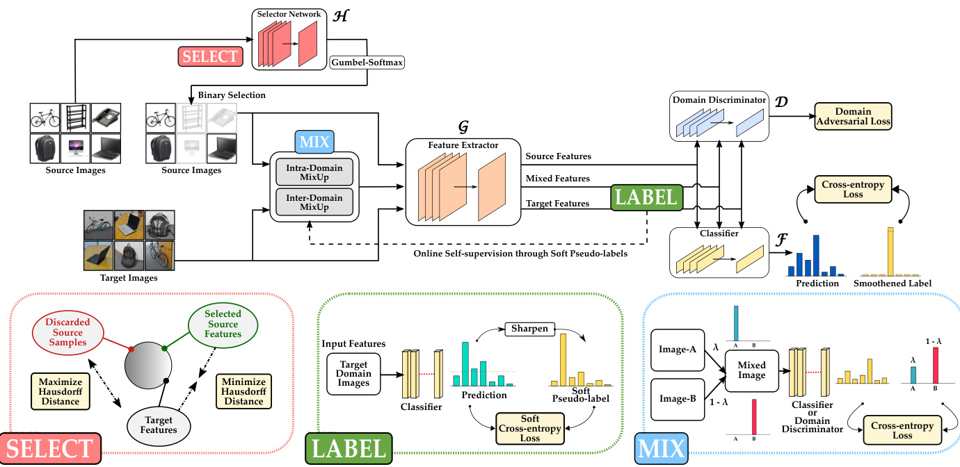
Figure 2: Illustration of our proposed framework. Our framework consists of a feature extractor $\mathcal{G}$ which maps the images to a common latent feature space, a classifier network $\mathcal{F}$ to provide class-wise predictions, a domain disc rim in at or $\mathcal{D}$ to reduce domain discrepancy, and a selector network $\mathcal{H}$ for discarding outlier source samples (“Select”) to mitigate the problem of negative transfer in partial domain adaptation. Our approach also comprises of two additional modules namely “Label” and “Mix” that works in conjunction with the “Select” module to ensure the disc rim inability and domain invariance of the latent space. Given a mini-batch of source and target domain images, all the components are optimized jointly in an iterative manner. See Section 3 for more details. Best viewed in color.
图 2: 我们提出的框架示意图。该框架包含一个将图像映射到公共潜在特征空间的特征提取器 $\mathcal{G}$、一个提供类别预测的分类器网络 $\mathcal{F}$、一个用于减少域差异的域判别器 $\mathcal{D}$,以及一个用于剔除异常源样本("Select")以缓解部分域适应中负迁移问题的选择器网络 $\mathcal{H}$。我们的方法还包含两个额外模块——"Label"和"Mix",它们与"Select"模块协同工作,确保潜在空间的可判别性和域不变性。给定一个源域和目标域图像的小批量样本,所有组件以迭代方式联合优化。详见第3节。建议彩色查看。
Mixup Regular iz ation. Mixup regular iz ation [53] or its variants [1, 45] that train models on virtual examples constructed as convex combinations of pairs of inputs and labels are recently used to improve the generalization of neural networks. A few recent methods apply Mixup, but mainly for UDA to stabilize domain disc rim in at or [48, 49, 51] or to smoothen the predictions [30]. Our proposed SLM strategy can be regarded as an extension of this line of research by introducing both intra-domain and inter-domain mixup not only to stabilize the disc rim in at or but also to guide the classifier in enriching the intrinsic structure of the latent space to solve the more challenging PDA task.
Mixup 正则化。Mixup 正则化 [53] 及其变体 [1, 45] 通过在输入和标签对的凸组合构建的虚拟样本上训练模型,近年来被用于提升神经网络的泛化能力。部分最新方法采用 Mixup,但主要应用于无监督域适应 (UDA) 以稳定域判别器 [48, 49, 51] 或平滑预测结果 [30]。我们提出的 SLM 策略可视为该研究方向的延伸,通过引入域内和域间混合 (mixup),不仅稳定判别器,还引导分类器丰富潜在空间的内在结构,以解决更具挑战性的部分域适应 (PDA) 任务。
3. Methodology
3. 方法论
Partial domain adaptation aims to mitigate the domain shift and generalize the model to an unlabelled target domain with a label space which is a subset of that of the lb a eb lle ell de ds osuorucrec ed odmo amiani ns.a mFoplrems aallsy $\mathcal{D}{s o u r c e}={(\mathbf{x}{i}^{s},y_{i})}{i=1}^{N{S}}$ and unlabelled target domain samples as $\mathcal{D}{t a r g e t}={\mathbf{x}{i}^{t}}{i=1}^{N{T}}$ with label spaces $\mathcal{L}{s o u r c e}$ and $\mathcal{L}{t a r g e t}$ , respectively, where $\mathcal{L}{s o u r c e}\subsetneq\mathcal{L}{t a r g e t}$ . $N_{S}$ and $N_{T}$ represent the number of samples in source and target domain respectively. Let $p$ and $q$ represent the probability distribution of data in source and target domain respectively. In partial domain adaptation, we further have $p\neq q$ and $p_{\mathcal{L}{t a r g e t}}\neq q$ , where $p{\mathcal{L}{t a r g e t}}$ is the distribution of source domain data in $\mathcal{L}{t a r g e t}$ . Our goal is to develop an approach with the above given data to improve the performance of a model on $\mathcal{D}_{t a r g e t}$ .
部分域适应的目标是缓解域偏移,并将模型泛化到一个未标记的目标域,该目标域的标签空间是已标记源域标签空间的子集。形式上,将已标记源域样本表示为 $\mathcal{D}{source}={(\mathbf{x}{i}^{s},y_{i})}{i=1}^{N{S}}$,未标记目标域样本表示为 $\mathcal{D}{target}={\mathbf{x}{i}^{t}}{i=1}^{N{T}}$,其标签空间分别为 $\mathcal{L}{source}$ 和 $\mathcal{L}{target}$,其中 $\mathcal{L}{source}\subsetneq\mathcal{L}{target}$。$N_{S}$ 和 $N_{T}$ 分别表示源域和目标域的样本数量。设 $p$ 和 $q$ 分别表示源域和目标域数据的概率分布。在部分域适应中,进一步满足 $p\neq q$ 且 $p_{\mathcal{L}{target}}\neq q$,其中 $p{\mathcal{L}{target}}$ 是源域数据在 $\mathcal{L}{target}$ 中的分布。我们的目标是利用上述给定数据开发一种方法,以提升模型在 $\mathcal{D}_{target}$ 上的性能。
3.1. Approach Overview
3.1. 方法概述
Figure 2 illustrates an overview of our proposed approach. Our framework consists of a feature extractor $\mathcal{G}$ , a classifier network $\mathcal{F}$ , a domain disc rim in at or $\mathcal{D}$ and a selector network $\mathcal{H}$ . Our goal is to improve classification performance of the combined network $\mathcal{F}(\mathcal{G}(.))$ on $\mathcal{D}{t a r g e t}$ . While the feature extractor $\mathcal{G}$ maps the images to a common latent space, the task of classifier $\mathcal{F}$ is to output a probability distribution over the classes for a given feature from $\mathcal{G}$ . Given a feature from $\mathcal{G}$ , the disc rim in at or $\mathcal{D}$ helps in minimizing domain discrepancy by identifying the domain (either source or target) to which it belongs. The selector network $\mathcal{H}$ helps in reducing negative transfer by learning to identify outlier source samples from $\mathcal{D}{s o u r c e}$ using Gumbel-Softmax sampling [20]. On the other hand, label module utilizes predictions of $\mathcal{F}(\mathcal{G}(.))$ to obtain soft pseudo-labels for target samples. Finally, the mix module leverages both pseudolabeled target samples and source samples to generate augmented images for achieving domain invariance in the latent space. During training, for a mini-batch of images, all the components are trained jointly and during testing, we evaluate performance using classification accuracy of the network $\mathcal{F}(\mathcal{G}(.))$ on target domain data $\mathcal{D}_{t a r g e t}$ . The individual modules are discussed below.
图 2: 我们提出的方法概述。我们的框架包含特征提取器 $\mathcal{G}$、分类网络 $\mathcal{F}$、域判别器 $\mathcal{D}$ 和选择器网络 $\mathcal{H}$。我们的目标是提升组合网络 $\mathcal{F}(\mathcal{G}(.))$ 在 $\mathcal{D}{target}$ 上的分类性能。特征提取器 $\mathcal{G}$ 将图像映射到共同潜在空间,分类器 $\mathcal{F}$ 的任务是对来自 $\mathcal{G}$ 的特征输出类别概率分布。给定 $\mathcal{G}$ 的特征,判别器 $\mathcal{D}$ 通过识别其所属域(源或目标)来最小化域差异。选择器网络 $\mathcal{H}$ 通过使用 Gumbel-Softmax 采样 [20] 学习识别 $\mathcal{D}{source}$ 中的异常源样本,从而减少负迁移。标签模块利用 $\mathcal{F}(\mathcal{G}(.))$ 的预测为目标样本获取软伪标签。最后,混合模块结合伪标记目标样本和源样本生成增强图像,以实现潜在空间的域不变性。训练时,对于小批量图像,所有组件联合训练;测试时,我们通过 $\mathcal{F}(\mathcal{G}(.))$ 在目标域数据 $\mathcal{D}_{target}$ 上的分类准确率评估性能。各模块具体说明如下。
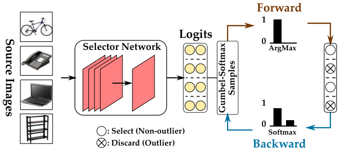
Figure 3: Learning with Gumbel Softmax Sampling. GumbelSoftmax trick used for enabling gradient-based optimization for discrete output space. Best viewed in color.
图 3: 使用Gumbel Softmax采样的学习过程。GumbelSoftmax技巧用于实现对离散输出空间的梯度优化。建议彩色查看。
3.2. Select Module
3.2. 选择模块
This module stands in the core of our framework with an aim to get rid of the outlier source samples in the source domain in order to minimize negative transfer in partial domain adaptation. Instead of using different heuristic ally designed criteria for weighting source samples, we develop a novel selector network $\mathcal{H}$ , that takes images from the source domain as input and makes instance-level binary predictions to obtain relevant source samples for adaptation, as shown in Figure 3. Specifically, the selector network $\mathcal{H}$ performs robust selection by providing a discrete binary output of either a 0 (discard) or $1:(s e l e c t)$ for each source sample, i.e., $\mathcal{H}:\mathcal{D}_{s o u r c e}\to{0,1}$ . We leverage Gumbel-Softmax operation to design the learning protocol of the selector network, as described next. Given the selection, we forward only the selected samples to the successive modules.
该模块是我们框架的核心,旨在剔除源域中的异常样本,以最小化部分域适应中的负迁移。不同于使用不同启发式设计的标准对源样本进行加权,我们开发了一种新颖的选择器网络 $\mathcal{H}$,它以源域图像作为输入,进行实例级别的二元预测,从而获取适用于适应的相关源样本,如图 3 所示。具体而言,选择器网络 $\mathcal{H}$ 通过为每个源样本提供离散的二元输出(0 表示丢弃,$1:(选择)$)来实现鲁棒选择,即 $\mathcal{H}:\mathcal{D}_{source}\to{0,1}$。我们利用 Gumbel-Softmax 操作设计选择器网络的学习协议,如下所述。根据选择结果,我们仅将选中的样本传递给后续模块。
Training using Gumbel-Softmax Sampling. Our select module makes decisions about whether a source sample belongs to an outlier class or not. However, the fact that the decision policy is discrete makes the network nondifferentiable and therefore difficult to optimize via standard back propagation. To resolve the non-different i ability and enable gradient descent optimization for the selector in an efficient way, we adopt Gumbel-Softmax trick [20, 29] and draw samples from a categorical distribution parameterized by $\alpha_{0}$ , $\alpha_{1}$ , where $\alpha_{0}$ , $\alpha_{1}$ are the output logits of the selector network for a sample to be selected and discarded respectively. As shown in Figure 3, the selector network $\mathcal{H}$ takes a batch of source images (say, $\boldsymbol{B}{s}$ of size $b$ ) as input, and outputs a two-dimensional matrix $\beta\in\mathbb{R}^{b\times2}$ , where each row corresponds to $[\alpha{0}$ $\alpha_{1}]$ for an image. We then draw i.i.d. samples $G_{0}$ , $G_{1}$ from $G u m b e l(0,1)~=~-l o g(-l o g(U))$ , where $U\sim$ Uniform $[0,1]$ and generate discrete samples in the forward pass as: $X=\arg\operatorname*{max}_{i}[\log\alpha_{i}+G_{i}]$ resulting in hard binary predictions, while during backward pass, we approximate gradients using continuous softmax relaxation as:
使用Gumbel-Softmax采样的训练。我们的选择模块负责判断源样本是否属于异常类。然而,离散决策策略会导致网络不可微分,从而难以通过标准反向传播进行优化。为解决不可微分性问题并高效实现选择器的梯度下降优化,我们采用Gumbel-Softmax技巧[20,29],从由$\alpha_{0}$、$\alpha_{1}$参数化的分类分布中采样,其中$\alpha_{0}$、$\alpha_{1}$分别表示选择器网络对样本被选中和丢弃的输出logits。如图3所示,选择器网络$\mathcal{H}$以一批源图像(例如大小为$b$的$\boldsymbol{B}{s}$)作为输入,输出一个二维矩阵$\beta\in\mathbb{R}^{b\times2}$,其中每行对应一张图像的$[\alpha{0}$ $\alpha_{1}]$。随后我们从$Gumbel(0,1)~=~-log(-log(U))$中独立同分布地采样$G_{0}$、$G_{1}$(其中$U\sim$均匀分布$[0,1]$),并在前向传播中生成离散样本:$X=\arg\operatorname*{max}_{i}[\log\alpha_{i}+G_{i}]$以得到硬二元预测结果;而在反向传播期间,我们使用连续softmax松弛近似梯度:

where $G_{i}$ ’s are i.i.d samples from standard Gumbel distribution $G u m b e l(0,1)$ and $\tau$ denotes temperature of softmax. When $\tau>0$ , the Gumbel-Softmax distribution is smooth and hence gradients can be computed with respect to logits $\alpha_{i}$ ’s to train the selector network using back propagation. As $\tau$ approaches 0, $\mathcal{{V}}_{i}$ becomes one-hot and discrete.
其中 $G_{i}$ 是来自标准Gumbel分布 $Gumbel(0,1)$ 的独立同分布样本,$\tau$ 表示softmax的温度参数。当 $\tau>0$ 时,Gumbel-Softmax分布是平滑的,因此可以通过反向传播计算关于logits $\alpha_{i}$ 的梯度来训练选择器网络。当 $\tau$ 趋近于0时,$\mathcal{V}_{i}$ 会变为one-hot且离散的形式。
Learning to Discard the Outlier Distribution. With the unsupervised nature of this decision problem, the design of the loss function for the selector network is challenging. We propose a novel Hausdorff distance-based triplet loss function for the select module which ensures that the selector network learns to distinguish between the outlier and the non-outlier distribution in the source domain. For a given batch of source domain images Dsbource and target domain images Dtbarget, each of size b, the selector results in two subsets of source samples $\mathcal{D}{s e l}={x\in\mathcal{D}{s o u r c e}^{b}:\mathcal{H}(x)=1}$ and $\mathcal{D}_{d i s}={x\in\mathcal{D}_{s o u r c e}^{b}:\mathcal{H}(x)=0}$ . The idea is to pull the selected source samples $\mathcal{D}_{s e l}$ & target samples $\mathcal{D}_{t a r g e t}^{b}$ closer while pushing discarded source samples $\mathcal{D}_{d i s}$ & Dtbarget apart in the output latent feature space of G. To achieve this, we formulate the loss function as follows:
学习剔除异常分布。由于该决策问题的无监督特性,为选择器网络设计损失函数具有挑战性。我们为选择模块提出了一种新颖的基于豪斯多夫距离(Hausdorff distance)的三元组损失函数,确保选择器网络能够区分源域中的异常与非异常分布。对于给定批次的源域图像$D_{s}^{b}$和目标域图像$D_{t}^{b}$(每批大小为b),选择器会生成两个源样本子集$\mathcal{D}{s e l}={x\in\mathcal{D}{s o u r c e}^{b}:\mathcal{H}(x)=1}$和$\mathcal{D}_{d i s}={x\in\mathcal{D}_{s o u r c e}^{b}:\mathcal{H}(x)=0}$。其核心思想是在生成器G的潜在特征空间中,拉近被选源样本$\mathcal{D}_{s e l}$与目标样本$\mathcal{D}_{t a r g e t}^{b}$的距离,同时推远被弃源样本$\mathcal{D}_{d i s}$与目标样本$D_{t}^{b}$的距离。为此,我们将损失函数构建如下:

where $d_{H}(X,Y)$ represents the average Hausdorff distance between the set of features $X$ and $Y$ . $\begin{array}{r l}{\mathcal{L}{r e g}}&{{}=}\end{array}$ $\begin{array}{r}{\lambda{r e g1}\sum_{x\in\mathcal{D}{s o u r c e}^{b}}\mathcal{H}(x)\log(\mathcal{H}(x))+\lambda{r e g2}{\sum_{\hat{p}}l_{e n t}(\hat{p})-}\end{array}$ $l_{e n t}\big(\hat{p}{m}\big)}$ , with $l{e n t}$ being the entropy loss, $\hat{p}$ is the Softmax prediction of $\mathcal{F}(\mathcal{G}(\mathcal{D}{t a r q e t}))$ and $\hat{p}{m}$ is mean prediction for the target domain. $\bar{\mathcal{L}}{r e g}$ is a regular iz ation to re- strict $\mathcal{H}$ from producing trivial all-0 or all-1 outputs as well as ensuring confident and diverse predictions by $\mathcal{F}(\mathcal{G}(.))$ for $\mathcal{D}{t a r g e t}$ . Note that only $\mathcal{D}_{s e l}$ is used to train the classifier, domain disc rim in at or and is utilised by other modules to perform subsequent operations. Furthermore, to avoid any interference from the backbone feature extractor $\mathcal{G}$ , we use a separate feature extractor for the select module, while making these decisions. In summary, the supervision signal for selector module comes from (a) the disc rim in at or directly, (b) through interactions with other modules via joint learning, and (c) the triplet loss using Hausdorff distance.
其中 $d_{H}(X,Y)$ 表示特征集 $X$ 和 $Y$ 之间的平均豪斯多夫距离。$\begin{array}{r l}{\mathcal{L}{r e g}}&{{}=}\end{array}$ $\begin{array}{r}{\lambda{r e g1}\sum_{x\in\mathcal{D}{s o u r c e}^{b}}\mathcal{H}(x)\log(\mathcal{H}(x))+\lambda{r e g2}{\sum_{\hat{p}}l_{e n t}(\hat{p})-}\end{array}$ $l_{e n t}\big(\hat{p}{m}\big)}$ ,其中 $l{e n t}$ 为熵损失,$\hat{p}$ 是 $\mathcal{F}(\mathcal{G}(\mathcal{D}{t a r q e t}))$ 的Softmax预测值,$\hat{p}{m}$ 是目标域的平均预测值。$\bar{\mathcal{L}}{r e g}$ 是一个正则化项,用于防止 $\mathcal{H}$ 产生全0或全1的平凡输出,同时确保 $\mathcal{F}(\mathcal{G}(.))$ 对 $\mathcal{D}{t a r g e t}$ 做出置信且多样化的预测。需要注意的是,只有 $\mathcal{D}_{s e l}$ 被用于训练分类器和域判别器,并被其他模块用于执行后续操作。此外,为避免骨干特征提取器 $\mathcal{G}$ 的干扰,我们在做出这些决策时使用了一个独立的特征提取器用于选择模块。综上所述,选择器模块的监督信号来自:(a) 判别器直接输出,(b) 通过与其他模块的联合学习交互,(c) 使用豪斯多夫距离的三元组损失。
3.3. Label Module
3.3. 标签模块
While our select module helps in removing source domain outliers, it fails to guarantee the disc rim inability of the latent space due to the absence of class-aware information in the target domain. Specifically, given our main objective is to improve the classification performance on target domain samples, it becomes essential for the classifier to learn confident decision boundaries in the target domain. To this end, we propose a label module that provides additional self-supervision for target domain samples. Motivated by the effectiveness of confidence guided self-training [56], we generate soft pseudo-labels for the target domain samples that efficiently attenuates the unwanted deviations caused by false and noisy one-hot pseudo-labels. For a target domain sample $\mathbf{x}{k}^{t}\in\mathcal{D}{t a r g e t}$ , the soft-pseudo-label $\hat{y}_{k}^{t}$ is computed as follows:
虽然我们的选择模块有助于去除源域异常值,但由于目标域缺乏类别感知信息,它无法保证潜在空间的判别性。具体而言,鉴于我们的主要目标是提升目标域样本的分类性能,分类器必须在目标域中学习到置信的决策边界。为此,我们提出了一个标签模块,为目标域样本提供额外的自监督。受置信度引导自训练[56]有效性的启发,我们为目标域样本生成软伪标签,有效减弱由错误和噪声独热伪标签引起的不良偏差。对于目标域样本$\mathbf{x}{k}^{t}\in\mathcal{D}{t a r g e t}$,其软伪标签$\hat{y}_{k}^{t}$的计算方式如下:

where $p(j|\mathbf{x}{i}^{t})=\mathcal{F}(\mathcal{G}(\mathbf{x}{i}^{t}))^{(j)}$ is the softmax probability of the classifier for class $j$ given $\mathbf{x}{i}^{t}$ as input, and $\alpha$ is a hyperparameter that controls the softness of the label. The soft pseudo-label $\hat{y}{i}^{t}$ is then used to compute the loss $\mathcal{L}{l a b e l}$ for a given batch of target samples $\mathcal{D}{t a r g e t}^{b}$ as follows:
其中 $p(j|\mathbf{x}{i}^{t})=\mathcal{F}(\mathcal{G}(\mathbf{x}{i}^{t}))^{(j)}$ 表示给定输入 $\mathbf{x}{i}^{t}$ 时分类器对类别 $j$ 的softmax概率,$\alpha$ 是控制标签软度的超参数。随后使用软伪标签 $\hat{y}{i}^{t}$ 计算目标样本批次 $\mathcal{D}{target}^{b}$ 的损失 $\mathcal{L}{label}$,公式如下:

where ${l}_{c e}(.)$ represents the cross-entropy loss.
其中 ${l}_{c e}(.)$ 表示交叉熵损失。
3.4. Mix Module
3.4. 混合模块
Learning a domain-invariant latent space is crucial for effective adaptation of a classifier from source to target domain. However, with limited samples per batch and after discarding the outlier samples, it becomes even more challenging in preventing over-fitting and learning domain invariant representation. To mitigate this problem, we apply MixUp [53] on the selected source samples and the target samples for discovering ingrained structures in establishing domain invariance. Given $\mathcal{D}{s e l}$ from select module and $\mathcal{D}{t a r g e t}^{b}$ with corresponding labels $\hat{y}^{t}$ from label module, we perform convex combinations of images belonging to these two sets on pixel-level in three different ways namely, interdomain, intra-source domain and intra-target domain to obtain the following sets of augmented data:
学习领域不变潜在空间对于分类器从源域到目标域的有效适配至关重要。然而,在每批样本数量有限且剔除离群样本后,防止过拟合并学习领域不变表征变得更具挑战性。为缓解该问题,我们对选定的源样本和目标样本应用MixUp [53]方法,通过三种不同方式(跨领域、源域内及目标域内)在像素级别对这两组样本进行凸组合,从而获得以下增强数据集:给定选择模块输出的$\mathcal{D}{s e l}$和标签模块提供的带预测标签$\hat{y}^{t}$的目标域数据$\mathcal{D}{t a r g e t}^{b}$。

where $(\mathbf{x}{i/j}^{s},y{i/j})\in\mathcal{D}{s e l}$ , while $\mathbf{x}{i/j}^{t}\in\mathcal{D}{t a r g e t}^{b}$ with $\hat{y}{i/j}^{t}$ being the corresponding soft-pseudo-labels. $\lambda$ is the mixratio randomly sampled from a beta distribution $B e t a(\alpha,\alpha)$ for $\alpha\in(0,\infty)$ . We use $\alpha=2.0$ in all our experiments.
其中 $(\mathbf{x}{i/j}^{s},y{i/j})\in\mathcal{D}{s e l}$,而 $\mathbf{x}{i/j}^{t}\in\mathcal{D}{t a r g e t}^{b}$ 且 $\hat{y}{i/j}^{t}$ 为对应的软伪标签。$\lambda$ 是从贝塔分布 $B e t a(\alpha,\alpha)$ 中随机采样的混合比例,其中 $\alpha\in(0,\infty)$。我们在所有实验中使用 $\alpha=2.0$。
Given the new augmented images, we utilize the new augmented images in training both the classifier $\mathcal{F}$ and the domain disc rim in at or $\mathcal{D}$ as follows:
给定这些新增的增强图像,我们在训练分类器 $\mathcal{F}$ 和域判别器 $\mathcal{D}$ 时使用这些新增强图像,具体如下:

where $\mathcal{L}{m i x.c l s}$ and $\mathcal{L}{m i x_d o m}$ represent loss for classifier and domain disc rim in at or respectively. Our mix strategy with the combined loss $\mathcal{L}_{m i x}$ not only helps to explore more intrinsic structures across domains leading to an invariant latent space, but also helps to stabilize the domain discriminator while bridging the distribution shift across domains.
其中 $\mathcal{L}{m i x.c l s}$ 和 $\mathcal{L}{m i x_d o m}$ 分别表示分类器和域判别器的损失。我们采用混合策略结合损失 $\mathcal{L}_{m i x}$ ,不仅能探索跨域更本质的结构以形成不变潜在空间,还能在弥合域间分布偏移的同时稳定域判别器。
Optimization. Besides the above three modules that are tailored for partial domain adaptation, we use the standard supervised loss on the labeled source data and domain adversarial loss as follows:
优化。除了上述三个针对部分域适配定制的模块外,我们在标记的源数据上使用标准监督损失和域对抗损失如下:

where $\mathcal{L}{a d v}$ is entropy-conditioned domain adversarial loss with weights $w^{s}$ and $w^{t}$ for source and target domain respectively [26]. The overall loss $\mathcal{L}{t o t a l}$ is
其中 $\mathcal{L}{a d v}$ 是带权重的熵条件域对抗损失,$w^{s}$ 和 $w^{t}$ 分别对应源域和目标域的权重 [26]。总体损失 $\mathcal{L}{t o t a l}$ 为

where $\mathcal{L}{s e l e c t}$ , $\mathcal{L}{l a b e l}$ , and $\mathcal{L}_{m i x}$ are given by Equations (2), (4), and (6) respectively, where we have included the corresponding weight coefficient hyper parameters. We integrate all the modules into one framework, as shown in Figure 2 and train the network jointly for partial domain adaptation.
其中 $\mathcal{L}{s e l e c t}$ 、$\mathcal{L}{l a b e l}$ 和 $\mathcal{L}_{m i x}$ 分别由公式 (2) 、(4) 和 (6) 给出,其中我们已包含相应的权重系数超参数。如图 2 所示,我们将所有模块集成到一个框架中,并联合训练网络以实现部分域适应。
4. Experiments
4. 实验
We conduct extensive experiments to show that our SLM framework outperforms many competing approaches to achieve the new state-of-the-art on several PDA benchmark datasets. We also perform comprehensive ablation experiments and feature visualization s to verify the effectiveness of different components in detail.
我们进行了大量实验,证明我们的SLM框架在多个PDA基准数据集上超越了众多竞争方法,达到了新的最优性能。同时通过全面的消融实验和特征可视化,详细验证了各模块的有效性。
4.1. Experimental Setup
4.1. 实验设置
Datasets. We evaluate our approach using four datasets under PDA setting, namely Office31 [38], Office-Home [44], ImageNet-Caltech and VisDA-2017 [36]. Office31 contains
数据集。我们在PDA设置下使用四个数据集评估我们的方法,分别是Office31 [38]、Office-Home [44]、ImageNet-Caltech和VisDA-2017 [36]。Office31包含
4,110 images of 31 classes from three distinct domains, namely Amazon (A), Webcam (W) and DSLR (D). Following [9], we select 10 classes shared by Office31 and Caltech256 [14] as target categories. Office-Home is a challenging dataset that contains images from four domains: Artistic images (Ar), Clipart images (Cl), Product images $(\mathrm{Pr})$ and Real-World images (Rw). We follow [9] to select the first 25 categories (in alphabetic order) in each domain as target classes. ImageNet-Caltech is a challenging dataset that consists of two subsets, ImageNet1K (I) [37] and Caltech256 (C) [14]. While source domain contains 1,000 and 256 classes for ImageNet and Caltech respectively, each target domain contains only 84 classes that are common across both domains. VisDA-2017 is a large-scale challenging dataset with 12 categories across 2 domains: one consists photo-realistic images or real images (R), and the other comprises of and synthetic 2D renderings of 3D models (S). We select the first 6 categories (in alphabetical order) in each of the domain as the target categories[22]. More details are included in the Appendix.
来自三个不同领域的31个类别共4,110张图像,分别是Amazon (A)、Webcam (W)和DSLR (D)。按照[9]的方法,我们选择Office31和Caltech256 [14]共有的10个类别作为目标类别。Office-Home是一个具有挑战性的数据集,包含来自四个领域的图像:艺术图像(Ar)、剪贴画图像(Cl)、产品图像$(\mathrm{Pr})$和真实世界图像(Rw)。我们按照[9]的方法选择每个领域按字母顺序排列的前25个类别作为目标类别。ImageNet-Caltech是一个具有挑战性的数据集,由两个子集组成:ImageNet1K (I) [37]和Caltech256 (C) [14]。虽然源域分别为ImageNet和Caltech包含1,000和256个类别,但每个目标域仅包含两个领域共有的84个类别。VisDA-2017是一个大规模挑战性数据集,包含跨越2个领域的12个类别:一个领域由照片级真实感图像或真实图像(R)组成,另一个领域由3D模型的合成2D渲染图像(S)组成。我们选择每个领域按字母顺序排列的前6个类别作为目标类别[22]。更多细节见附录。
Baselines. We compare our approach with several methods that fall into two main categories: (1) popular UDA methods (e.g., DANN [12], CORAL [42]) including recent methods like CAN [21] and SPL [47] which have shown stateof-the-art performance on UDA setup, (2) existing partial domain adaptation methods including PADA [4], SAN [3], ETN [5], and DRCN [22]. We also compare with the recent state-of-the-art methods, RTNet [9] that uses reinforcement learning for source dataset selection, and $\mathrm{{BA}^{3}U S}$ [24] which uses source samples to augment the target domain in partial domain adaptation.
基线方法。我们将所提方法与两大类方法进行对比:(1) 主流无监督域适应 (UDA) 方法 (如 DANN [12]、CORAL [42]),包括近期在UDA任务中表现优异的CAN [21]和SPL [47];(2) 现有部分域适应方法,包括PADA [4]、SAN [3]、ETN [5]和DRCN [22]。同时对比了最新前沿方法:采用强化学习进行源数据集选择的RTNet [9],以及通过源样本增强目标域的 $\mathrm{{BA}^{3}U S}$ [24]。
Implementation Details. We use ResNet-50 [15] as the backbone network for the feature extractor while we use ResNet-18 for the selector network, initialized with ImageNet [37] pretrained weights. All the weights are shared by both the source and target domain images except that of the BatchNorm layers, for which we use Domain-Specific Batch Normalization [6]. In Eqn. 2 we set $\lambda_{s},\lambda_{r e g1}$ and $\lambda_{r e g2}$ as 0.01, 10.0 and 0.1, respectively. We use a margin value of 100.0 in all our experiments. We use gradient reversal layer (GRL) for adversarial ly training the discriminator. We set $\tau=1.0$ in Eqn. 1, $\alpha=0.1$ in Eqn. 3, and $\lambda~=~0.0$ for the GRL as initial values and gradually anneal $\tau$ and $\alpha$ down to 0 while increase $\lambda$ to 1.0 during the training, as in [20]. Additionally, we use label-smoothing for all the losses for the feature extractor involving source domain images as in [23, 32], with $\epsilon=0.2$ . We use SGD for optimization with momentum $_{1=0.9}$ while a weight decay of 1e-3 and 5e-4 for the selector network and the other networks respectively. We use an initial learning rate of 5e3 for the selector and the classifier, while 5e-4 for the rest of the networks and decay it following a cosine annealing strategy. We use a batch size of 64 for Office31 and VisDA
实现细节。我们使用ResNet-50 [15]作为特征提取器的主干网络,而选择器网络则采用ResNet-18,均使用ImageNet [37]预训练权重进行初始化。除BatchNorm层采用域特定批归一化[6]外,所有权重在源域和目标域图像间共享。在公式2中,我们设定$\lambda_{s}$、$\lambda_{reg1}$和$\lambda_{reg2}$分别为0.01、10.0和0.1。所有实验均采用100.0的边界值。对抗训练判别器时使用了梯度反转层(GRL)。初始值设定为:公式1中$\tau=1.0$,公式3中$\alpha=0.1$,GRL的$\lambda=0.0$;随后按照[20]的方法,在训练过程中逐步将$\tau$和$\alpha$衰减至0,同时将$\lambda$增至1.0。此外,对于涉及源域图像的特征提取器损失函数,我们采用[23,32]的标签平滑技术($\epsilon=0.2$)。优化器使用带动量($_{1=0.9}$)的SGD,选择器网络权重衰减为1e-3,其他网络为5e-4。选择器和分类器的初始学习率为5e3,其余网络为5e-4,并按余弦退火策略衰减。Office31和VisDA数据集的批处理大小设为64。
| 方法 | A→W | D→W | W→D | A→D | D→A | W→A | 平均 |
|---|---|---|---|---|---|---|---|
| ResNet-50 | 76.5±0.3 | 99.2±0.2 | 97.7±0.1 | 87.5±0.2 | 87.2±0.1 | 84.1±0.3 | 88.7 |
| DANN | 62.8±0.6 | 71.6±0.4 | 65.6±0.5 | 65.1±0.7 | 78.9±0.3 | 79.2±0.4 | 70.5 |
| CORAL | 52.1±0.5 | 65.2±0.2 | 64.1±0.7 | 58.0±0.5 | 73.1±0.4 | 77.9±0.3 | 65.1 |
| ADDA | 75.7±0.2 | 95.4±0.2 | 99.9±0.1 | 83.4±0.2 | 83.6±0.1 | 84.3±0.1 | 87.0 |
| RTN | 75.3 | 97.1 | 98.3 | 66.9 | 85.6 | 85.7 | 84.8 |
| CDAN+E | 80.5±1.2 | 99.0±0.0 | 98.1±0.0 | 77.1±0.9 | 93.6±0.1 | 91.7±0.0 | 90.0 |
| JDDA | 73.5±0.6 | 93.1±0.3 | 89.3±0.2 | 76.4±0.4 | 77.6±0.1 | 82.8±0.2 | 82.1 |
| CAN | 84.4±0.0 | 92.0±1.4 | 94.7±1.7 | 84.9±0.9 | 85.6±1.0 | 86.4±0.8 | 88.0 |
| PADA | 86.3±0.4 | 99.3±0.1 | 100.0±0.0 | 90.4±0.1 | 91.3±0.2 | 92.6±0.1 | 93.3 |
| SAN | 93.9±0.5 | 99.3±0.5 | 99.4±0.1 | 94.3±0.3 | 94.2±0.4 | 88.7±0.4 | 95.0 |
| IWAN | 89.2±0.4 | 99.3±0.3 | 99.4±0.2 | 90.5±0.4 | 95.6±0.3 | 94.3±0.3 | 94.7 |
| ETN | 93.4±0.3 | 99.3±0.1 | 99.2±0.2 | 95.5±0.4 | 95.4±0.1 | 91.7±0.2 | 95.8 |
| DRCN | 88.1 | 100.0 | 100.0 | 86.0 | 95.6 | 95.8 | 94.3 |
| RTNet | 95.1±0.3 | 100.0±0.0 | 100.0±0.0 | 97.8±0.1 | 93.9±0.1 | 94.1±0.1 | 96.8 |
| RTNetadv | 96.2±0.3 | 100.0±0.0 | 100.0±0.0 | 97.6±0.1 | 92.3±0.1 | 95.4±0.1 | 96.9 |
| BA3US | 99.0±0.3 | 100.0±0.0 | 98.7±0.0 | 99.4±0.0 | 94.8±0.1 | 95.0±0.1 | 97.8 |
| SLM(本文) | 99.8±0.2 | 100.0±0.0 | 99.8±0.3 | 98.7±0.0 | 96.1±0.1 | 95.9±0.0 | 98.4 |
Table 1: Performance on Office31. Numbers show the accuracy $(%)$ of different methods on partial domain adaptation setting. We highlight the best and second best method on each transfer task. While the upper section shows the results of some popular unsupervised domain adaptation approaches, the lower section shows results of existing partial domain adaptation methods. SLM achieves the best performance on 4 out of 6 transfer tasks including the best average performance among all compared methods.
表 1: Office31数据集上的性能。数字表示不同方法在部分域自适应设置下的准确率 $(%)$ 。我们标出了每个迁移任务中表现最佳和次佳的方法。上半部分展示了一些流行的无监督域自适应方法的结果,下半部分则展示了现有部分域自适应方法的结果。SLM在6个迁移任务中的4个上取得了最佳性能,包括所有对比方法中的最佳平均表现。
2017 while a batch size of 128 is used for Office-Home and ImageNet-Caltech. We report average classification accuracy and standard deviation over 3 random trials. All the codes were implemented using PyTorch [34].
2017年,对于Office-Home和ImageNet-Caltech数据集,我们使用128的批量大小。我们报告了3次随机试验的平均分类准确率和标准差。所有代码均使用PyTorch [34]实现。
4.2. Results and Analysis
4.2. 结果与分析
Table 1 shows the results of our proposed method and other competing approaches on the Office31 dataset. We have the following key observations. (1) As expected, the popular UDA methods including the recent CAN [21], fail to outperform the simple no adaptation model (ResNet50), which implies that they suffer from negative transfer due to the presence of outlier source samples in partial domain adaptation. (2) Overall, our SLM framework outperforms all the existing PDA methods by achieving the best results on 4 out of 6 transfer tasks. Among PDA methods, $\mathrm{{BA}^{3}U S}$ [24] is the most competitive. However, SLM still outperforms it $(97.8%$ vs $98.4%$ ) due to our two novel components working in concert with the removal of outliers: enhancing disc rim inability of the latent space via iterative pseudo-labeling of target domain samples and learning domain-invariance through mixup regular iz at ions. (3) Our approach performed remarkably well on transfer tasks where the number of source domain images is very small compared to the target domain, e.g., on $\mathrm{D}\rightarrow\mathrm{A}$ , SLM outperforms $\mathrm{{BA}^{3}U S}$ by $1.3%$ . This shows that our method improves generalization ability of source classifier in target domain while reducing negative transfer.
表1: 我们提出的方法与其他竞争方法在Office31数据集上的结果对比。我们得出以下关键观察:(1) 正如预期,包括最新CAN[21]在内的流行无监督域适应(UDA)方法未能超越简单的无适应模型(ResNet50),这表明在部分域适应场景中,由于异常源样本的存在,这些方法遭受了负迁移效应。(2) 总体而言,我们的SLM框架在6个迁移任务中的4个上取得最佳结果,优于所有现有PDA方法。在PDA方法中,$\mathrm{{BA}^{3}U S}$[24]最具竞争力,但SLM仍以$(97.8%$ vs $98.4%)$的优势超越它,这归功于我们两个协同工作的创新组件:通过目标域样本的迭代伪标记增强潜在空间判别力,以及通过混合正则化学习域不变特征。(3) 我们的方法在源域图像数量远少于目标域的迁移任务(如$\mathrm{D}\rightarrow\mathrm{A}$)上表现尤为突出,SLM以$1.3%$的优势超越$\mathrm{{BA}^{3}U S}$,这表明我们的方法在减少负迁移的同时,提升了源分类器在目标域的泛化能力。
On the challenging Office-Home dataset, our proposed approach obtains very competitive performance, with an average accuracy of $76.0%$ on this dataset (Table 2). Our method obtains the best on 6 out of 12 transfer tasks. Table 3 summarizes the results on ImageNet-Caltech and VisDA-2017 datasets. Our approach once again achieves the best performance, outperforming the next competitive method by a margin of about $2.8%$ and $18.9%$ on ImageNet-Caltech and VisDA-2017 datasets respectively. Especially for task $\mathrm{S}\rightarrow\mathrm{R}$ on VisDA-2017 dataset, our approach significantly outperforms SAFN [50] and DRCN [22] by an increase of $24.1%$ and $33.5%$ respectively. Note that on the most challenging VisDA-2017 dataset, our approach is still able to distill more positive knowledge from the synthetic to the real domain despite significant domain gap across them. In summary, SLM outperforms the existing PDA methods on all four datasets, showing the effectiveness of our approach in not only identifying the most relevant source classes but also learning more transferable features for partial domain adaptation.
在具有挑战性的Office-Home数据集上,我们提出的方法取得了极具竞争力的性能,平均准确率达到$76.0%$(表2)。在12个迁移任务中,我们的方法在6个任务上表现最佳。表3总结了ImageNet-Caltech和VisDA-2017数据集上的结果。我们的方法再次实现了最佳性能,在ImageNet-Caltech和VisDA-2017数据集上分别以约$2.8%$和$18.9%$的优势超越次优方法。特别是在VisDA-2017数据集的$\mathrm{S}\rightarrow\mathrm{R}$任务上,我们的方法显著优于SAFN[50]和DRCN[22],分别提高了$24.1%$和$33.5%$。值得注意的是,在最具挑战性的VisDA-2017数据集上,尽管存在显著的领域差距,我们的方法仍能从合成领域向真实领域提取更多正向知识。总之,SLM在所有四个数据集上都超越了现有的PDA方法,表明我们的方法不仅能识别最相关的源类别,还能为部分领域自适应学习更具可迁移性的特征。
Table 2: Performance on Office-Home. We highlight the best and second best method on each task. While the upper section shows results of unsupervised domain adaptation approaches, the lower section shows results of existing partial domain adaptation methods.SLM achieves the best average performance among all compared methods. See supplementary material for standard deviation of each task.
表 2: Office-Home 数据集性能对比。我们标出了每项任务中表现最佳和次佳的方法。上半部分展示无监督域适应方法的结果,下半部分展示现有部分域适应方法的结果。SLM 在所有对比方法中取得了最佳平均性能。各任务标准差详见补充材料。
| Method | Ar→Cl | Ar→Pr | Ar→Rw | Cl→Ar | Cl→Pr | Cl→Rw | Pr→Ar | Pr→Cl | Pr→Rw | Rw→Ar | Rw→Cl | Rw→Pr |
|---|---|---|---|---|---|---|---|---|---|---|---|---|
| ResNet-50 | 47.2 | 66.8 | 76.9 | 57.6 | 58.4 | 62.5 | 59.4 | 40.6 | 75.9 | 65.6 | 49.1 | 75.8 |
| DANN | 43.2 | 61.9 | 72.1 | 52.3 | 53.5 | 57.9 | 47.2 | 35.4 | 70.1 | 61.3 | 37.0 | 71.7 |
| CORAL | 38.2 | 55.6 | 65.9 | 48.4 | 52.5 | 51.3 | 48.9 | 32.6 | 67.1 | 63.8 | 35.9 | 69.8 |
| ADDA | 45.2 | 68.8 | 79.2 | 64.6 | 60.0 | 68.3 | 57.6 | 38.9 | 77.5 | 70.3 | 45.2 | 78.3 |
| RTN | 49.4 | 64.3 | 76.2 | 47.6 | 51.7 | 57.7 | 50.4 | 41.5 | 75.5 | 70.2 | 51.8 | 74.8 |
| CDAN+E | 47.5 | 65.9 | 75.7 | 57.1 | 54.1 | 63.4 | 59.6 | 44.3 | 72.4 | 66.0 | 49.9 | 72.8 |
| JDDA | 45.8 | 63.9 | 74.1 | 51.8 | 55.2 | 60.3 | 53.7 | 38.3 | 72.6 | 62.5 | 43.3 | 71.3 |
| SPL | 46.4 | 70.5 | 77.2 | 61.0 | 65.2 | 73.2 | 64.3 | 44.7 | 79.1 | 69.5 | 58.0 | 79.8 |
| PADA | 53.2 | 69.5 | 78.6 | 61.7 | 62.7 | 60.9 | 56.4 | 44.6 | 79.3 | 74.2 | 55.1 | 77.4 |
| SAN | 44.4 | 68.7 | 74.6 | 67.5 | 65.0 | 77.8 | 59.8 | 44.7 | 80.1 | 72.2 | 50.2 | 78.7 |
| IWAN | 53.9 | 54.5 | 78.1 | 61.3 | 48.0 | 63.3 | 54.2 | 52.0 | 81.3 | 76.5 | 56.8 | 82.9 |
| ETN | 60.4 | 76.5 | 77.2 | 64.3 | 67.5 | 75.8 | 69.3 | 54.2 | 83.7 | 75.6 | 56.7 | 84.5 |
| SAFN | 58.9 | 76.3 | 81.4 | 70.4 | 73.0 | 77.8 | 72.4 | 55.3 | 80.4 | 75.8 | 60.4 | 79.9 |
| DRCN | 54.0 | 76.4 | 83.0 | 62.1 | 64.5 | 71.0 | 70.8 | 49.8 | 80.5 | 77.5 | 59.1 | 79.9 |
| RTNet | 62.7 | 79.3 | 81.2 | 65.1 | 68.4 | 76.5 | 70.8 | 55.3 | 85.2 | 76.9 | 59.1 | 83.4 |
| RTNetadv | 63.2 | 80.1 | 80.7 | 66.7 | 69.3 | 77.2 | 71.6 | 53.9 | 84.6 | 77.4 | 57.9 | 85.5 |
| BA?US | 60.6 | 83.2 | 88.4 | 71.8 | 72.8 | 83.4 | 75.5 | 61.6 | 86.5 | 79.3 | 62.8 | 86.1 |
| SLM(Ours) | 61.1 | 84.0 | 91.4 | 76.5 | 75.0 | 81.8 | 74.6 | 55.6 | 87.8 | 82.3 | 57.8 | 83.5 |
Table 3: Performance on ImageNet-Caltech and VisDA-2017. Our SLM performs the best on both datasets.
表 3: ImageNet-Caltech 和 VisDA-2017 数据集上的性能表现。我们的 SLM 在两个数据集上均取得最佳结果。
| 方法 | I→C | C→I | 平均 | R→S | S→R | 平均 |
|---|---|---|---|---|---|---|
| ResNet-50 | 69.7±0.8 | 71.3±0.7 | 70.5 | 64.3 | 45.3 | 54.8 |
| DAN | 71.6 | 66.5 | 69.0 | 68.4 | 47.6 | 58.0 |
| DANN | 68.7 | 52.9 | 60.8 | 73.8 | 51.0 | 62.4 |
| ADDA | 70.6 | |||||
| RTN | 71.8±0.5 | 69.3±0.4 | 70.3 | 72.9 | - | 61.5 |
| 72.2 | 68.3 | |||||
| CDAN+E | 72.5±0.1 | 72.0±0.1 | 72.2 | - | 50.0 | |
| PADA | 75.0±0.4 | 72.8 | 76.5 | - | 65.0 | |
| SAN | 70.5±0.4 | 76.5 | 53.5 | |||
| 77.8±0.4 | 75.3±0.4 | 69.7 | 49.9 | |||
| IWAN | 78.1±0.4 | 73.3±0.5 | 75.7 | 71.3 | 48.6 | |
| ETN | 83.2±0.2 | 74.9±0.4 | 79.1 | - | - | |
| SAFN | - | - | 67.7±0.5 | |||
| DRCN | 75.3 | 78.9 | 77.1 | 73.2 | 58.2 | 65.7 |
| SLM(本文) | 82.3±0.1 | 81.4±0.6 | 81.9 | 77.5±0.8 | 91.7±0.8 | 84.6 |
4.3. Ablation Studies
4.3. 消融实验
We perform the following experiments to test the effectiveness of the proposed modules including the effect of number of target classes on different datasets.
我们通过以下实验来测试所提出模块的有效性,包括目标类别数量对不同数据集的影响。
Effectiveness of Individual Modules. We conduct experiments to investigate the importance of our three unique modules on three datasets. E.g. On Office-Home, as seen from Table 4, while the Select only module improves the vanilla performance by $8%$ , addition of Label and Mix modules progressively improves the result to obtain the best performance of $76.0%$ . This corroborates the fact that both disc rim inability and invariance of the latent space plays a crucial role in partial domain adaptation in addition to removal of source domain outlier samples.
各模块的有效性。我们通过实验探究三个独特模块在三个数据集上的重要性。以Office-Home数据集为例,如表4所示:仅使用Select模块就能将基线性能提升8%,而逐步加入Label和Mix模块后,性能持续提升至最佳水平76.0%。这验证了潜在空间的判别性与不变性(discriminability and invariance)对部分域适应的重要性,其作用不亚于移除源域离群样本。
Effectiveness of Discrete Selection. The adverse effects of negative transfer motivated us to adopt a strong form of discrete selection of relevant source samples instead of a weak form of filtering using soft-weights as adopted in many prior works [4, 5]. In Table 5, we replaced the weighting module in PADA [4] with our stronger Select module (PADA w/ SEL) and obtained an average accuracy of $94.9%$ on Office31 which is $1.6%$ higher than the original PADA method, showing the superior selection of our Select module. We also adopted the class-weighting $(\gamma)$ scheme from PADA [4] and used threshold ing on top of it (SLM w/ $\mathrm{{W+T}},$ ) to replace the Select module in SLM and obtained $94.0%$ average accuracy. The $4.4%$ drop shows the ineffectiveness of filtering outliers solely based on the target predictions and the importance of having a dedicated Select module which takes decisions as a function of the source samples.
离散选择的有效性。负迁移的负面影响促使我们采用一种强形式的相关源样本离散选择方法,而非如许多先前工作[4,5]所采用的基于软权重过滤的弱形式。在表5中,我们将PADA[4]的加权模块替换为更强的选择模块(PADA w/ SEL),在Office31数据集上获得了94.9%的平均准确率,比原始PADA方法高出1.6%,这表明我们的选择模块具有优越性。我们还采用了PADA[4]的类别加权(γ)方案,并在此基础上添加阈值处理(SLM w/ W+T)来替代SLM中的选择模块,获得了94.0%的平均准确率。4.4%的下降表明仅基于目标预测过滤异常值的低效性,以及需要专用选择模块(其决策以源样本为函数)的重要性。
Comparison with Varying Number of Target Classes. We compare different methods by varying the target label space. In Figure 4, SLM consistently obtains the best results indicating its advantage in alleviating negative transfer by removing outlier source samples. SLM outperforms all the compared methods even in the case of completely shared space (A31 W31), which shows that it does not discard relevant samples incorrectly when there are no outlier classes.
目标类别数量变化的对比
我们通过改变目标标签空间来比较不同方法。在图4中,SLM始终获得最佳结果,表明其通过移除异常源样本缓解负迁移的优势。即使在完全共享空间(A31 W31)的情况下,SLM也优于所有对比方法,这表明当没有异常类别时,它不会错误地丢弃相关样本。
Table 4: Effectiveness of Different Modules on Office-Home Dataset. Our proposed approach achieves the best performance with all the modules working jointly for learning disc rim i native invariant features in partial domain adaptation.
表 4: Office-Home数据集上不同模块的有效性。我们提出的方法在所有模块共同作用下学习部分域适应的判别性不变特征时取得了最佳性能。
| 选择 | 标签 | 混合 | Office-Home | Ar→ClArPrArRwCl→→ArCl→PrCl→RwPr→ArPr→ClPr→RwRw→ArPr→ClPr→Rw | 平均 | |||||||||
|---|---|---|---|---|---|---|---|---|---|---|---|---|---|---|
| × | × | × | 44.2 | 61.6 | 75.9 | 54.6 | 55.2 | 65.0 | 51.0 | 37.3 | 69.6 | 64.8 | 42.4 | 71.4 |
| × | × | × | 50.6 | 72.9 | 79.2 | 65.4 | 67.2 | 71.7 | 60.8 | 46.7 | 77.1 | 71.9 | 49.4 | 77.0 |
| × | 56.1 | 82.4 | 89.8 | 74.2 | 73.0 | 81.6 | 70.8 | 48.4 | 87.0 | 80.1 | 53.1 | 81.7 | ||
| 61.1 | 84.0 | 91.4 | 76.5 | 75.0 | 81.8 | 74.6 | 55.6 | 87.8 | 82.3 | 57.8 | 83.5 |
| 方法 | A→W | D→W | W→D | A→D | D→A | W→A | 平均 |
|---|---|---|---|---|---|---|---|
| PADA | 86.3 | 99.3 | 100.0 | 90.4 | 91.3 | 92.6 | 93.3 |
| PADA w/SEL | 91.8 | 99.3 | 96.6 | 93.8 | 94.2 | 93.5 | 94.9 |
| SLM w/W+T | 90.8 | 99.7 | 98.7 | 93.0 | 91.8 | 90.2 | 94.0 |
| SLM | 99.8 | 100.0 | 99.8 | 98.7 | 96.1 | 95.9 | 98.4 |

Table 5: Effectiveness of Discrete Selection. Figure 4: Performance by varying the number of target classes on $\mathbf A{\to}\mathbf W$ task from Office31 dataset. Best viewed in color.
表 5: 离散选择的有效性
图 4: 在 Office31 数据集 $\mathbf A{\to}\mathbf W$ 任务中,目标类别数量变化对性能的影响。建议彩色查看。
Effectiveness of Different Mixup. We examine the effect of mixup regular iz ation on both domain disc rim in at or and classifier on Office-Home dataset. With mixup regularizations working for both disc rim in at or and classifier, the average performance on Office-Home dataset is $76.0%$ . By removing mixup regular iz ation from the training of domain disc rim in at or, it decreases to $73.6%$ . Similarly, by removing mixup regular iz ation from the classifier training, the average performance becomes $73.9%$ . This corroborates the fact that our Mix strategy not only helps to explore intrinsic structures across domains, but also helps to stabilize the domain disc rim in at or. We also explored CutMix [52] as an alternative mixing strategy, which can result with new images with information from both the domains are also expected to work well resonating with our motivation. In Table 6, we replace MixUp with CutMix (SLM w/ CutMix) in the Mix module and obtain an average accuracy of $98.0%$ on Office31 almost similar to that using MixUp $(98.4%)$ . We also tried adding CutMix in addition to MixUp (SLM w/ MixUp $^+$ Cutmix) and obtain a similar value of $98.4%$ , with a slight improvement in $\mathbf{W}{\rightarrow}\mathbf{D}$ task.
不同混合策略的有效性。我们在Office-Home数据集上考察了混合正则化(mixup regularization)对域判别器(domain discriminator)和分类器的效果。当混合正则化同时作用于域判别器和分类器时,Office-Home数据集的平均性能达到$76.0%$。若从域判别器训练中移除混合正则化,性能降至$73.6%$;类似地,从分类器训练中移除混合正则化后,平均性能变为$73.9%$。这证实了我们的混合策略(Mix strategy)不仅能帮助探索跨域内在结构,还能稳定域判别器。我们还探索了CutMix[52]作为替代混合策略,该策略通过融合两域信息生成新图像,与我们的动机相契合。在表6中,我们将Mix模块中的MixUp替换为CutMix(SLM w/ CutMix),在Office31数据集上获得$98.0%$的平均准确率,与使用MixUp的$(98.4%)$几乎相当。我们还尝试在MixUp基础上叠加CutMix(SLM w/ MixUp$^+$Cutmix),获得相近的$98.4%$结果,其中$\mathbf{W}{\rightarrow}\mathbf{D}$任务略有提升。
Table 6: Performance using CutMix.
表 6: 使用 CutMix 的性能表现。
| Method | A→W1 | DW | W→DA→DD→A | 1W→A | Average | ||
|---|---|---|---|---|---|---|---|
| SLMw/CutMix | 99.6 | 100.0 | 100.0 | 97.4 | 95.7 | 95.5 | 98.0 |
| SLMw/MixUp | 99.8 | 100.0 | 99.8 | 98.7 | 96.1 | 95.9 | 98.4 |
| SLMw/MixUp+CutMix | 99.8 | 100.0 | 100.0 | 98.7 | 96.1 | 95.9 | 98.4 |
| 距离 | A→DW→A | Cl → Pr Rw → Pr |
|---|---|---|
| dist(Ssel, T) | 0.999 0.893 | 0.819 |
| dist(Sdis, T) | 1.013 1.144 | 0.947 1.418 |
Table 7: Wasser stein Distance between Domains. Table shows values for two randomly sampled tasks from Office-31 and OfficeHome. The values are normalized by assuming the distance for $\mathrm{dist}(\mathbf{S}{a l l},\mathbf{T})$ to be equal to 1.000, where $\mathrm{S}{a l l}$ represents all source samples for the corresponding tasks.
表 7: 域间Wasserstein距离。表格展示了从Office-31和OfficeHome数据集中随机采样的两个任务的距离值。这些数值通过假设$\mathrm{dist}(\mathbf{S}{a l l},\mathbf{T})$的距离等于1.000进行归一化处理,其中$\mathrm{S}{a l l}$表示对应任务的所有源样本。
Distance between Domains. Following [9], we compute the Wasser stein distance between the probability distribution of target samples (T) with that of selected $(S_{s e l})$ and discarded samples $(\mathrm{S}{d i s})$ by the selector network. Table 7 shows that dis $\mathbf{\Psi}=(\mathbf{S}{s e l},\mathbf{T})$ is smaller than d $\mathrm{i}s\mathrm{t}(\mathbf{S}{a l l},\mathbf{T})$ , while $\mathrm{dist}(\mathbf{S}{d i s},\mathbf{T})$ is greater than $\mathrm{dist}(\mathrm{S}_{a l l},\mathrm{T})$ on two randomly sampled adaptation tasks from Office31 and Office-Home. The results affirm that samples selected by our selector network are closer to target domain while the discarded samples are very dissimilar to the target domain.
域间距离。根据[9],我们计算了目标样本(T)的概率分布与选择器网络选中的样本$(S_{sel})$及丢弃样本$(\mathrm{S}{dis})$之间的Wasserstein距离。表7显示,在Office31和Office-Home的两个随机采样适配任务中,$\mathbf{\Psi}=(\mathbf{S}{sel},\mathbf{T})$的距离小于$d\mathrm{is}\mathrm{t}(\mathbf{S}{all},\mathbf{T})$,而$\mathrm{dist}(\mathbf{S}{dis},\mathbf{T})$大于$\mathrm{dist}(\mathrm{S}_{all},\mathrm{T})$。结果表明,选择器网络选中的样本更接近目标域,而被丢弃的样本与目标域差异显著。
Additional Ablation Analysis. We provide additional ablation analyses including effect of Hausdorff distance, soft pseudo-labels, results with different backbones, feature visu aliz at ions using t-SNE [28], etc. in the Appendix.
额外消融分析。我们在附录中提供了更多消融分析,包括豪斯多夫距离(Hausdorff distance)的影响、软伪标签(soft pseudo-labels)、不同主干网络的结果、使用t-SNE[28]的特征可视化等内容。
5. Conclusion
5. 结论
In this paper, we propose an end-to-end framework for learning disc rim i native invariant feature representation while preventing negative transfer in partial domain adaptation. While our select module facilitates the identification of relevant source samples for adaptation, the label module enhances the disc rim inability of the latent space by utilizing pseudo-labels for the target domain samples. The mix module uses mixup regular iz at ions jointly with the other two strategies to enforce domain invariance in latent space.
本文提出了一种端到端框架,用于学习具有区分性的不变特征表示,同时防止部分域自适应中的负迁移。其中选择模块有助于识别相关源样本进行适配,标签模块通过为目标域样本生成伪标签来增强潜在空间的区分性。混合模块则结合其他两种策略,利用混合正则化在潜在空间中强制实现域不变性。
Acknowledgement. This work is supported by the SERB Grant SRG/2019/001205 and the Defense Advanced Research Projects Agency (DARPA) under Contract No. FA8750-19-C-1001. Any opinions, findings and conclusions or recommendations expressed in this material are those of the author(s) and do not necessarily reflect the views of the Defense Advanced Research Projects Agency.
致谢。本研究由SERB资助项目SRG/2019/001205和美国国防高级研究计划局(DARPA)合同号FA8750-19-C-1001支持。本文所述观点、发现、结论或建议仅代表作者立场,未必反映美国国防高级研究计划局的观点。
References
参考文献
A. Dataset Details
A. 数据集详情
We evaluate the performance of our approach on several benchmark datasets for partial domain adaptation, namely Office31 [38], Office-Home [44], ImageNet-Caltech and VisDA-2017 [36]. The following are the detailed descriptions of the above datasets:
我们在多个部分域自适应基准数据集上评估了所提出方法的性能,包括Office31 [38]、Office-Home [44]、ImageNet-Caltech和VisDA-2017 [36]。以下是上述数据集的详细描述:

Figure 5: Sampled Images from Office31 Dataset. Each row from top to bottom corresponds to the domains Amazon, Dslr and Webcam, respectively. The images in the same column belong to the same class. Best viewed in color.
图 5: Office31数据集采样图像。从上到下每行分别对应Amazon、Dslr和Webcam三个域。同一列中的图像属于同一类别。建议彩色查看。

Figure 6: Sampled Images from Office-Home Dataset. Each row from top to bottom corresponds to the domains Art, Clipart, Product and RealWorld, respectively. The images in the same column belong to the same class. Best viewed in color.
图 6: Office-Home数据集采样图像。从上到下每行分别对应Art(艺术)、Clipart(剪贴画)、Product(产品)和RealWorld(真实世界)领域。同一列中的图像属于同一类别。建议彩色查看。

Figure 7: Sampled Images from ImageNet-Caltech Dataset. The top row corresponds to the ImageNet domain, while the bottom row to the Caltech domain. The images in the same column belong to the same class. Best viewed in color.
图 7: ImageNet-Caltech 数据集的采样图像。顶行对应 ImageNet 域,底行对应 Caltech 域。同一列中的图像属于同一类别。建议彩色查看。
ImageNet-Caltech. This large-scale dataset consists of two datasets (ImageNet1K [37] (I) & Caltech256 [14] (C)) as two separate domains and consist of over 14 million images combined. 2 transfer tasks are formed for this dataset. While source domain contains 1,000 and 256 classes for ImageNet and Caltech respectively, each target domain contains only 84 classes that are common across both domains. As it is a general practice to use ImageNet pretrained weights for network initialization, we use the validation set images when using ImageNet as the target domain. Number of Outlier Classes $=172$ for $\scriptstyle\mathrm{C}\to\mathrm{I}$ , 916 for $\mathrm{I}{\rightarrow}\mathrm{C}$ . Figure 7 displays a gallery of sample images for this dataset. The datasets are publicly available to download at:
ImageNet-Caltech。该大规模数据集由两个独立域的数据集(ImageNet1K [37] (I)和Caltech256 [14] (C))组成,合计包含超过1400万张图像。基于此数据集构建了2个迁移任务。当源域分别包含ImageNet的1000个类别和Caltech的256个类别时,每个目标域仅包含两个域共有的84个类别。由于通常采用ImageNet预训练权重进行网络初始化,当ImageNet作为目标域时我们使用其验证集图像。离群类别数在$\scriptstyle\mathrm{C}\to\mathrm{I}$任务中为$172$,在$\mathrm{I}{\rightarrow}\mathrm{C}$任务中为916。图7展示了该数据集的样本图像库。数据集可通过以下链接公开下载:
http://www.image-net.org/ http://www.vision.caltech.edu/Image_ Datasets/Caltech256/.
http://www.image-net.org/ http://www.vision.caltech.edu/Image_Datasets/Caltech256/

Figure 8: Sampled Images from VisDA-2017 Dataset. The top row corresponds to the Synthetic domain, while the bottom row to the Real domain. The images in the same column belong to the same class. Best viewed in color.
图 8: VisDA-2017数据集中的采样图像。顶行对应合成(Synthetic)域,底行对应真实(Real)域。同一列中的图像属于同一类别。建议彩色查看。
Figure 8 displays a gallery of sample images for this dataset. The dataset is publicly available to download at: http://ai.bu.edu/visda-2017/#download.
图 8: 展示了该数据集的样本图像库。该数据集可公开下载,地址为:http://ai.bu.edu/visda-2017/#download。
B. Implementation Details
B. 实现细节
The training pipeline pseudo-code for SLM is shown in Algorithm 1. Following are the detailed description of the implementation we follow for various components of the framework:
SLM的训练流程伪代码如算法1所示。以下是我们在框架各组件实现中遵循的详细说明:
Feature Extractor $(\mathcal G)$ . We use ResNet-50 [15] backbone for the feature extractor. The overall structure of ResNet50 is Initial Layers, Layer-1, Layer-2, Layer-3, Layer-4, AvgPool, Fc. The model is initialized with ImageNet [37] pretrained weights. Additionally, we add a bottleneck layer of width 256 just after the AvgPool layer to obtain the features and replace all the BatchNorm layers with Domain-Specific BatchNormalization [6] layers. All the layers till Layer-3 are frozen and only the rest of the layers are fine-tuned.
特征提取器 $(\mathcal G)$。我们采用ResNet-50[15]作为特征提取器的主干网络,其整体结构依次为初始层、Layer-1、Layer-2、Layer-3、Layer-4、AvgPool和Fc。该模型使用ImageNet[37]预训练权重进行初始化。此外,我们在AvgPool层后添加了宽度为256的瓶颈层以获取特征,并将所有BatchNorm层替换为领域特定批归一化(Domain-Specific BatchNormalization)[6]层。Layer-3及之前的所有层均被冻结,仅对后续层进行微调。
Selector Network $(\mathcal{H})$ . We use a ResNet-18 [15] network with the $\mathrm{F}\subset$ layer replaced with a binary-length fully connected layer as the selector network in our framework. The network is initialized with ImageNet pretrained weights and all the layers are trained while optimization.
选择器网络 $(\mathcal{H})$。我们采用ResNet-18 [15]作为框架中的选择器网络,将其 $\mathrm{F}\subset$ 层替换为二元全连接层。该网络使用ImageNet预训练权重初始化,并在优化过程中训练所有层。
Classifier $(\mathcal{F})$ . The final $\mathrm{F}\subset$ layer of ResNet-50 described above is replaced with a task-specific fully-connected layer to form the classifier network of our framework.
分类器 $(\mathcal{F})$。上述 ResNet-50 的最终 $\mathrm{F}\subset$ 层被替换为特定任务的全连接层,构成我们框架的分类器网络。
Domain Disc rim in at or $(\mathcal{D})$ . A three-layer fully-connected network is used as the domain disc rim in at or network. It takes the 256-length features obtained from the feature extractor as input. The adversarial training is incorporated using a gradient reversal layer (GRL).
域判别器 $(\mathcal{D})$。一个三层全连接网络被用作域判别器网络。它以从特征提取器获得的256维特征作为输入,并通过梯度反转层(GRL)实现对抗训练。
Hyper parameters. All the networks are optimised using mini-batch stochastic gradient descent with a momentum of 0.9. A batch size of 64 is used for Office31 and VisDA2017 while a batch size of 128 is used for Office-Home and ImageNet-Caltech. For feature extractor an initial learning rate of 5e-5 for the convolutional layers while an initial learning rate of 5e-4 for all the fully-connected layers is used. For the selector network and the domain discriminator an initial learning rate of 5e-3 and 5e-4 are used respectively. The learning rates are decayed following a cosineannealing strategy as the training progresses. The best models are captured by obtaining the performance on a valida- tion set. We do NOT follow the ten-crop technique [4, 5], to improve the performance in the inference phase. We obtain the best hyper parameters using grid search. All the experiments were averaged over three runs, which used random seed values of 1, 2, and 3 respectively.
超参数 (Hyper parameters)。所有网络均使用小批量随机梯度下降法进行优化,动量 (momentum) 设为0.9。Office31和VisDA2017数据集采用64的批量大小 (batch size),Office-Home和ImageNet-Caltech数据集采用128的批量大小。特征提取器中,卷积层初始学习率设为5e-5,全连接层初始学习率设为5e-4。选择器网络和域判别器分别采用5e-3和5e-4的初始学习率。学习率随训练进程采用余弦退火 (cosineannealing) 策略衰减。通过在验证集上的表现来选取最佳模型。我们未采用十裁剪技术 (ten-crop technique) [4,5] 来提升推理阶段性能。通过网格搜索 (grid search) 确定最佳超参数。所有实验均进行三次随机种子值为1/2/3的独立运行并取平均值。
Hardware and Software Details. All the experiments were conducted using a single NVIDIA Tesla $\mathrm{V}100\mathrm{-}\mathrm{D}\mathrm{G}\mathrm{X}S$ GPU with 32 GigaBytes of memory, equipped with a Intel(R) Xeon(R) CPU E5-2698 $\begin{array}{r l}{\mathtt{v}4}&{{}\mathtt{(d~}2.20\mathtt{G H z}}\end{array}$ . We used PyTorch v1.4.0, Python v3.6.10 to implement the codes.
硬件与软件配置详情。所有实验均在配备32GB内存的NVIDIA Tesla $\mathrm{V}100\mathrm{-}\mathrm{D}\mathrm{G}\mathrm{X}S$ GPU和Intel(R) Xeon(R) CPU E5-2698 $\begin{array}{r l}{\mathtt{v}4}&{{}\mathtt{(d~}2.20\mathtt{G H z}}\end{array}$ 的硬件环境下完成,采用PyTorch v1.4.0与Python语言 v3.6.10实现代码。
Algorithm 1 The training pipeline for SLM
算法 1: SLM训练流程
9: end for
9: 结束循环
C. Additional Experimental Results
C. 补充实验结果
Results on Office-Home Dataset. In Table 8, along with the performance accuracies, we have included the standard deviation for each adaptation task for the Office-Home dataset, as promised in Table-2 of the main paper.
Office-Home数据集结果。在表8中,除了性能准确率外,我们还按照主论文表2的承诺,包含了Office-Home数据集每个适应任务的标准差。
Effectiveness on Different Backbone Networks. To show that the proposed framework is backbone-agnostic, i.e., it provides the best performance irrespective of the architecture of the feature extractor, we conduct experiments using a VGG-16 [41] backbone for the feature extractor. We report the results on the transfer tasks from the Office31 dataset in Table 9 and compare it with the current state-ofthe-art methods. Our method outperforms the previously best results by a margin of $\mathbf{3.0%}$ on average and achieves new state-of-the-art results. This confirms that our proposed framework for partial domain adaptation is robust with respect to the change of backbone network.
在不同骨干网络上的有效性。为证明所提框架与骨干网络无关(即无论特征提取器采用何种架构都能提供最佳性能),我们使用VGG-16[41]作为特征提取器骨干进行实验。表9展示了Office31数据集迁移任务的结果,并与当前最优方法进行对比。我们的方法以平均$\mathbf{3.0%}$的优势超越此前最佳结果,创造了新的性能标杆。这证实了所提出的部分域适应框架对骨干网络变更具有鲁棒性。
Table 8: Performance on Office-Home. We highlight the best and second best method on each task. While the upper section shows results of unsupervised domain adaptation approaches, the lower section shows results of existing partial domain adaptation methods.SLM achieves the best average performance among all compared methods.
表 8: Office-Home性能对比。我们在每个任务上标出最佳和次佳方法。上半部分展示无监督域适应方法的结果,下半部分展示现有部分域适应方法的结果。SLM在所有对比方法中取得最佳平均性能。
| Method | Ar→Cl | Ar→Pr | Ar→Rw | Cl→Ar | Cl→Pr | Cl→Rw | Pr→Ar | Pr→Cl | Pr→Rw | Rw→Ar | Rw→Cl | Rw→Pr | Average |
|---|---|---|---|---|---|---|---|---|---|---|---|---|---|
| ResNet-50 | 47.2±0.2 | 66.8±0.3 | 76.9±0.5 | 57.6±0.2 | 58.4±0.1 | 62.5±0.3 | 59.4±0.3 | 40.6±0.2 | 75.9±0.3 | 65.6±0.1 | 49.1±0.2 | 75.8±0.4 | 61.3 |
| DANN | 43.2±0.5 | 61.9±0.2 | 72.1±0.4 | 52.3±0.4 | 53.5±0.2 | 57.9±0.1 | 47.2±0.3 | 35.4±0.1 | 70.1±0.3 | 61.3±0.2 | 37.0±0.2 | 71.7±0.3 | 55.3 |
| CORAL | 38.2±0.1 | 55.6±0.3 | 65.9±0.2 | 48.4±0.4 | 52.5±0.1 | 51.3±0.2 | 48.9±0.3 | 32.6±0.1 | 67.1±0.2 | 63.8±0.4 | 35.9±0.2 | 69.8±0.1 | 52.5 |
| ADDA | 45.2 | 68.8 | 79.2 | 64.6 | 60.0 | 68.3 | 57.6 | 38.9 | 77.5 | 70.3 | 45.2 | 78.3 | 62.8 |
| RTN | 49.4 | 64.3 | 76.2 | 47.6 | 51.7 | 57.7 | 50.4 | 41.5 | 75.5 | 70.2 | 51.8 | 74.8 | 59.3 |
| CDAN+E | 47.5 | 65.9 | 75.7 | 57.1 | 54.1 | 63.4 | 59.6 | 44.3 | 72.4 | 66.0 | 49.9 | 72.8 | 60.7 |
| JDDA | - | - | - | - | - | - | - | - | - | - | - | 71.3±0.1 | 57.7 |
| SPL | 45.8±0.4 | 63.9±0.2 | 74.1±0.3 | 51.8±0.2 | 55.2±0.3 | 60.3±0.2 | 53.7±0.2 | 38.3±0.1 | 72.6±0.2 | 62.5±0.1 | 43.3±0.3 | 79.8±0.0 | 65.7 |
| PADA | 53.2±0.2 | 69.5±0.1 | 78.6±0.1 | 61.7±0.2 | 62.7±0.3 | 60.9±0.1 | 56.4±0.5 | 44.6±0.2 | 79.3±0.1 | 74.2±0.1 | 55.1±0.3 | 77.4±0.2 | 64.5 |
| SAN | - | 68.7 | 74.6 | - | 65.0 | - | - | - | 80.1 | 72.2 | 50.2 | 78.7 | 65.3 |
| IWAN | 44.4 | - | 78.1 | 67.5 | - | 77.8 | 59.8 | 44.7 | - | 76.5 | 56.8 | 82.9 | 63.6 |
| ETN | 53.9 | 54.5 | - | 61.3 | 48.0 | 63.3 | 54.2 | 52.0 | 81.3 | - | - | - | 70.5 |
| SAFN | - | 60.4±0.3 | 76.5±0.2 | - | - | - | - | - | 83.7±0.2 | 75.6±0.3 | 56.7±0.2 | 84.5±0.3 | 71.8 |
| DRCN | 54.0 | 76.4 | 83.0 | 62.1 | 64.5 | 71.0 | 70.8 | 49.8 | 80.5 | 77.5 | 59.1 | 79.9 | 69.0 |
| RTNet | 62.7±0.1 | 79.3±0.2 | 81.2±0.1 | 65.1±0.1 | 68.4±0.3 | 76.5±0.1 | - | 55.3±0.1 | 85.2±0.3 | 76.9±0.2 | 59.1±0.2 | 83.4±0.3 | 72.0 |
| RTNetadv | 63.2±0.1 | 80.1±0.2 | 80.7±0.1 | 66.7±0.1 | 69.3±0.2 | 77.2±0.2 | 71.6±0.3 | 53.9±0.3 | 84.6±0.1 | 77.4±0.2 | 57.9±0.3 | 85.5±0.1 | 72.3 |
| BA3US | 60.6±0.5 | 83.2±0.1 | 88.4±0.2 | 71.8±0.2 | 72.8±1.1 | 83.4±0.6 | 75.5±0.2 | 61.6±0.4 | 86.5±0.2 | 79.3±0.7 | 62.8±0.5 | 86.1±0.3 | 76.0 |
Table 9: Performance on Office31 with VGG-16 backbone. Numbers show the accuracy $(%)$ of different methods on partial domain adaptation setting. We highlight the best and second best method on each transfer task. Our proposed framework, SLM achieves the best performance on 4 out of 6 transfer tasks including the best average performance among all compared methods.
| 方法 | A→W | D→W | W→D | A→D | D→A | W→A | 平均 |
|---|---|---|---|---|---|---|---|
| VGG-16 [41] (ICLR'15) | 60.3±0.8 | 98.0±0.6 | 99.4±0.4 | 76.4±0.5 | 73.0±0.6 | 79.1±0.5 | 81.0 |
| PADA [4] (ECCV'18) | 86.1±0.4 | 100.0±0.0 | 100.0±0.0 | 81.7±0.3 | 93.0±0.2 | 95.3±0.3 | 92.5 |
| SAN [3] (CVPR'18) | 83.4±0.4 | 99.3±0.5 | 100.0±0.0 | 90.7±0.2 | 87.2±0.2 | 91.9±0.4 | 92.1 |
| IWAN [54] (CVPR'18) | 82.9±0.3 | 79.8±0.3 | 88.5±0.2 | 91.0±0.3 | 89.6±0.2 | 93.4±0.2 | 87.5 |
| ETN [5] (CVPR'19) | 85.7±0.2 | 100.0±0.0 | 100.0±0.0 | 89.4±0.2 | 95.9±0.2 | 92.3±0.2 | 93.9 |
| SLM (Ours) | 92.0±0.1 | 99.8±0.2 | 99.6±0.5 | 98.1±0.0 | 96.1±0.0 | 96.0±0.1 | 96.9 |
表 9: 基于VGG-16骨干网络的Office31性能表现。数值表示不同方法在部分域适应设置下的准确率(%)。我们标出了每个迁移任务中表现最佳和次佳的方法。我们提出的SLM框架在6个迁移任务中的4个上取得了最佳性能,并且在所有对比方法中获得了最高的平均性能。
works the best in all cases.
在所有情况下表现最佳。
Effectiveness of Individual Modules. In Section 4.3 of the main paper, we discussed the importance of the proposed three unique modules on Office-Home dataset. Here, we extend the experiments to Office31 and VisDA-2017 and provide the performance on the transfer tasks in Table 10. Similar to the results on Office-Home dataset, our approach with all the three modules (Select, Label and Mix) working jointly, works the best on both datasets.
各模块的有效性。在正文第4.3节中,我们讨论了所提出的三个独特模块在Office-Home数据集上的重要性。此处我们将实验扩展到Office31和VisDA-2017数据集,并在表10中提供了迁移任务的性能表现。与Office-Home数据集的结果类似,当三个模块(Select、Label和Mix)共同工作时,我们的方法在两个数据集上都取得了最佳效果。
Effectiveness of Hausdorff Distance. We investigate the effect of Hausdorff distance (Eqn. 2 in the main paper) in selector network training and find that removing it lowers down performance from $76.0%$ to $73.7%$ on Office-Home dataset, showing its importance in guiding the selector to discard the outlier source samples for effective reduction in negative transfer. We provide the individual performance of all the transfer tasks on Office-Home dataset in Table 11, which shows that our approach with Hausdorff distance loss
Hausdorff距离的有效性。我们研究了Hausdorff距离(主论文中的公式2)在selector network训练中的作用,发现去除该距离会使Office-Home数据集上的性能从$76.0%$降至$73.7%$,这表明其在指导selector剔除异常源样本以减少负迁移方面具有重要作用。表11展示了我们在Office-Home数据集上所有迁移任务的个体性能,结果表明采用Hausdorff距离损失的方案...
Effectiveness of Soft Pseudo-Labels. We also test the effec ti ve ness of soft pseudo-labels by replacing them with hard pseudo-labels for the target samples and observe that the average performance decreases from $76.0%$ to $72.0%$ on Office-Home dataset. This confirms that soft pseudo-labels are critical in attenuating the unwanted deviations caused by the false and noisy hard pseudo-labels. We provide the performance on each of the transfer tasks from Office-Home in Table 12.
软伪标签的有效性。我们还通过将目标样本的软伪标签替换为硬伪标签来测试其效果,发现在Office-Home数据集上平均性能从$76.0%$降至$72.0%$。这证实了软伪标签对于减少由错误和噪声硬伪标签引起的不良偏差至关重要。表12展示了Office-Home各迁移任务的具体性能表现。
Effectiveness of Different MixUp. We examined the effect of mixup regular iz ation on both domain disc rim in at or and classifier separately in Section 4.3 of the main paper. We concluded that our Mix strategy not only helps to explore intrinsic structures across domains, but also helps to stabilize the domain disc rim in at or. Here, we provide the corresponding performance on each of the transfer tasks of Office-Home in Table 13.
不同MixUp策略的有效性。我们在主论文第4.3节分别分析了mixup正则化对领域判别器(domain discriminator)和分类器的影响,结果表明我们的Mix策略不仅能帮助探索跨领域的内在结构,还能稳定领域判别器。表13展示了Office-Home数据集各迁移任务上的对应性能表现。
Table 10: Effectiveness of Different Modules on Office31 and VisDA-2017 Datasets. Our proposed approach achieves the best performance with all the modules working jointly for learning disc rim i native invariant features in partial domain adaptation.
表 10: 不同模块在Office31和VisDA-2017数据集上的有效性。我们提出的方法在所有模块共同作用下学习部分域适应的判别性不变特征时取得了最佳性能。
| Select | Label | Mix | Office31 | VisDA-2017 | ||||||||
|---|---|---|---|---|---|---|---|---|---|---|---|---|
| × | × | × | 88.0 | 98.3 | 95.8 | 88.8 | 84.5 | 80.2 | 89.3 | 57.7 56.4 | 平均 57.0 | |
| √ | 91.8 | 99.3 | 96.6 93.8 | 94.2 | 93.5 | 94.9 | 69.0 | 68.4 | 68.7 | |||
| √ | √ | × | 92.4 | 99.9 | 99.2 94.9 | 95.5 | 93.8 | 96.0 | 77.2 | 84.8 | 81.0 | |
| √ | 99.8 | 100.0 | 99.8 | 98.7 96.1 | 95.9 | 98.4 | 77.5 | 91.7 | 84.6 |
Table 11: Effectiveness of Hausdorff Triplet Loss on Office-Home Dataset. The table shows the performance of the framework without (top-row) and with (bottom-row) the inclusion of the Hausdorff distance triplet loss. The results highlight the importance of the Hausdorff distance loss in our proposed framework.
表 11: Hausdorff三元组损失在Office-Home数据集上的有效性。该表展示了框架在不包含(首行)和包含(末行)Hausdorff距离三元组损失时的性能表现,结果凸显了Hausdorff距离损失在我们提出框架中的重要性。
| Ar→Cl | Ar→Pr | Ar→Rw | Cl→Ar | Cl→Pr | Cl→Rw | Pr→Ar | Pr→Cl | Pr→Rw | Rw→Ar | Rw→Cl | Rw→Pr | |
|---|---|---|---|---|---|---|---|---|---|---|---|---|
| W/oHausdorffLoss | 56.2 | 83.1 | 90.3 | 72.6 | 71.5 | 80.8 | 71.4 | 51.6 | 84.8 | 82.5 | 57.5 | 81.7 |
| Ours(SLM) | 61.1 | 84.0 | 91.4 | 76.5 | 75.0 | 81.8 | 74.6 | 55.6 | 87.8 | 82.3 | 57.8 | 83.5 |
Table 12: Effectiveness of Soft Pseudo-labels on Office-Home Dataset. Table shows the performance of the framework when we replace the soft pseudo-labels with hard pseudo-labels (top-row) for the target samples. The results justify that the soft pseudo-labels are critical for our framework and attenuate unwanted deviations caused by hard pseudo-labels.
表 12: Office-Home数据集上软伪标签的有效性。本表展示了当我们将目标样本的软伪标签替换为硬伪标签(首行)时框架的性能表现。结果表明软伪标签对我们的框架至关重要,并能减轻硬伪标签带来的不良偏差。
| Average | |
|---|---|
| W/HardPseudo-labels | 52.5 |
| Ours(SLM) | 61.1 |
Table 13: Effectiveness of Different MixUp on Office-Home Dataset. The table shows the performance of the framework with the exclusion of mixup regular iz ation from the domain disc rim in at or (top-row) and the class si fier (middle-row). The final row shows the results of the proposed SLM framework, which provides the best performance confirming the importance of our Mix strategy.
表 13: Office-Home数据集上不同MixUp策略的效果。该表格展示了框架在排除领域判别器 (top-row) 和分类器 (middle-row) 的mixup正则化后的性能。最后一行展示了提出的SLM框架的结果,其提供了最佳性能,证实了我们Mix策略的重要性。
| Ar→Cl | Ar→Pr | Ar→Rw | Cl→Ar | Cl→Pr | Cl→Rw | Pr→Ar | Pr→Cl | Pr→Rw | Rw→Ar | Rw→Pr | Rw→Cl | 平均 | |
|---|---|---|---|---|---|---|---|---|---|---|---|---|---|
| NoDomainDiscriminatorMixUp | 56.2 | 81.5 | 90.0 | 74.0 | 71.8 | 80.3 | 72.2 | 50.9 | 86.3 | 79.8 | 58.0 | 82.0 | 73.6 |
| No ClassifierMixUp | 57.8 | 82.9 | 88.5 | 75.1 | 73.6 | 79.3 | 69.0 | 54.9 | 86.6 | 79.8 | 57.6 | 81.2 | 73.9 |
| Ours (SLM) | 61.1 | 84.0 | 91.4 | 76.5 | 75.0 | 81.8 | 74.6 | 55.6 | 87.8 | 82.3 | 57.8 | 83.5 | 76.0 |
D. Qualitative Results
D. 定性结果
Feature Visualization s. We use t-SNE [28] to visual- ize the features learned using different components of our SLM framework. We choose an UDA setup (similar to DANN [12]) as a vanilla method and add different modules one-by-one to visualize their individual contribution in learning disc rim i native features for partial domain adaptation. As seen from Figure 9, the feature space for vanilla setup lacks dic rim inability for both source and target features. The disc rim inability improves for both source as well as target features as we add “Select” and “Label” to the Vanilla setup. The best results are obtained when all three modules “Select”, “Label” and “Mix” i.e., SLM are added and trained jointly in an end-to-end manner.
特征可视化。我们使用t-SNE [28]来可视化通过SLM框架不同组件学习到的特征。选择UDA设置(类似DANN [12])作为基础方法,逐步添加不同模块以观察它们对部分域适应中判别特征学习的独立贡献。如图9所示,基础设置的特征空间对源特征和目标特征都缺乏判别性。当在基础设置中加入"Select"和"Label"模块后,源特征和目标特征的判别性均得到提升。当同时加入"Select"、"Label"和"Mix"三个模块(即完整SLM)并以端到端方式联合训练时,获得了最佳效果。
E. Broader Impact and Limitations
E. 更广泛的影响与局限性
Our research can help reduce burden of collecting largescale supervised data in many real-world applications of visual classification by transferring knowledge from models trained on large broad datasets to specific datasets pos- sessing a domain shift. This scenario is quite common as large datasets (e.g. ImageNet [37]) can be used for training which contain a broader range of categories while our goal can be to transfer the knowledge to smaller datasets with a smaller number of categories. The positive impact that our work could have on society is in making technology more accessible for institutions and individuals that do not have rich resources for annotating newly collected datasets. We also believe our approach of selecting relevant source data would motivate the research community to extend it to various open-world problems and would help in training more general iz able models. Negative impacts of our research are difficult to predict, however, it shares many of the pitfalls associated with standard deep learning models such as susce pti bil it y to adversarial attacks and lack of interpret abl it y.
我们的研究通过将基于大型通用数据集训练的模型知识迁移到存在领域偏移的特定数据集,有助于减轻许多视觉分类实际应用中收集大规模监督数据的负担。这种情况相当常见,因为可以使用包含更广泛类别的大型数据集(如ImageNet [37])进行训练,而我们的目标是将知识迁移到类别较少的较小数据集。这项工作的积极社会影响在于,使资源有限无法对新收集数据集进行标注的机构和个人更易获得相关技术。我们相信,这种选择相关源数据的方法将推动研究界将其扩展到各种开放世界问题,并有助于训练更具泛化能力的模型。虽然研究的负面影响难以预测,但它与标准深度学习模型存在许多共性问题,例如易受对抗攻击和可解释性不足。

Figure 9: Feature Visualization s using t-SNE. Plots show visualization of our approach with different modules on $\mathbf{A}{\to}\mathbf{W}.$ , $\mathbf{A}{\xrightarrow{}}\mathbf{D}$ , $\mathrm{W}{\to}\mathrm{A}$ , and $\mathrm{D}{\rightarrow}\mathrm{A}$ tasks rep ect iv ely (top to down) from Office31 dataset. Blue and red dots represent source and target data respectively. As can be seen, features for both target as well as source domain become progressively disc rim i native and improve from left to right by adoption of our proposed modules. Best viewed in color.
图 9: 使用 t-SNE 的特征可视化。图表展示了我们在 Office31 数据集上 $\mathbf{A}{\to}\mathbf{W}$ 、 $\mathbf{A}{\xrightarrow{}}\mathbf{D}$ 、 $\mathrm{W}{\to}\mathrm{A}$ 和 $\mathrm{D}{\rightarrow}\mathrm{A}$ 任务(从上到下)采用不同模块的可视化效果。蓝点和红点分别代表源数据和目标数据。可以看出,通过采用我们提出的模块,目标域和源域的特征逐渐变得可区分,并呈现从左到右的改进效果。建议彩色查看。