Generative Pre training from Pixels
基于像素的生成式预训练 (Generative Pre-training from Pixels)
Mark Chen 1 Alec Radford 1 Rewon Child 1 Jeff $\mathbf{W}\mathbf{u}^{1}$ Heewoo Jun 1 Prafulla Dhariwal 1 David Luan 1 Ilya Sutskever
Mark Chen 1 Alec Radford 1 Rewon Child 1 Jeff $\mathbf{W}\mathbf{u}^{1}$ Heewoo Jun 1 Prafulla Dhariwal 1 David Luan 1 Ilya Sutskever
Abstract
摘要
Inspired by progress in unsupervised representation learning for natural language, we examine whether similar models can learn useful representations for images. We train a sequence Transformer to auto-regressive ly predict pixels, without incorporating knowledge of the 2D input structure. Despite training on low-resolution ImageNet without labels, we find that a GPT-2 scale model learns strong image representations as measured by linear probing, fine-tuning, and low-data classification. On CIFAR-10, we achieve $96.3%$ accuracy with a linear probe, outperforming a supervised Wide ResNet, and $99.0%$ accuracy with full finetuning, matching the top supervised pre-trained models. An even larger model trained on a mixture of ImageNet and web images is competitive with self-supervised benchmarks on ImageNet, achieving $72.0%$ top-1 accuracy on a linear probe of our features.
受自然语言无监督表征学习进展的启发,我们探究类似模型能否学习有效的图像表征。我们训练了一个序列Transformer (Transformer) 进行像素自回归预测,且未引入2D输入结构的先验知识。尽管在无标签的低分辨率ImageNet数据上训练,我们发现GPT-2规模的模型通过线性探测 (linear probing) 、微调和低数据分类评估,仍能学习到强大的图像表征。在CIFAR-10上,线性探测达到96.3%准确率(超越有监督Wide ResNet),全微调达到99.0%准确率(媲美顶级有监督预训练模型)。在ImageNet与网络图像混合数据上训练的更大模型,其线性探测特征达到72.0% top-1准确率,与ImageNet自监督基准性能相当。
1. Introduction
1. 引言
Unsupervised pre-training played a central role in the resurgence of deep learning. Starting in the mid 2000’s, approaches such as the Deep Belief Network (Hinton et al., 2006) and Denoising Auto encoder (Vincent et al., 2008) were commonly used in neural networks for computer vision (Lee et al., 2009) and speech recognition (Mohamed et al., 2009). It was believed that a model which learned the data distribution $P(X)$ would also learn beneficial features for the subsequent supervised modeling of $P(Y|X)$ (Lasserre et al., 2006; Erhan et al., 2010). However, advancements such as piecewise linear activation functions (Nair & Hinton, 2010), improved initialization s (Glorot & Bengio, 2010), and normalization strategies (Ioffe & Szegedy, 2015; Ba et al., 2016) removed the need for pre-training in order to achieve strong results. Other research cast doubt on the benefits of deep unsupervised representations and reported strong results using a single layer of learned features (Coates et al., 2011), or even random features (Huang et al., 2014; May et al., 2017). The approach fell out of favor as the state of the art increasingly relied on directly encoding prior structure into the model and utilizing abundant supervised data to directly learn representations (Krizhevsky et al., 2012; Graves & Jaitly, 2014). Retrospective study of unsupervised pre-training demonstrated that it could even hurt performance in modern settings (Paine et al., 2014).
无监督预训练在深度学习的复兴中扮演了核心角色。从2000年代中期开始,深度信念网络 (Hinton et al., 2006) 和去噪自编码器 (Vincent et al., 2008) 等方法被广泛应用于计算机视觉 (Lee et al., 2009) 和语音识别 (Mohamed et al., 2009) 的神经网络中。当时认为,学习数据分布 $P(X)$ 的模型也会为后续的监督建模 $P(Y|X)$ 学习到有益特征 (Lasserre et al., 2006; Erhan et al., 2010)。然而,分段线性激活函数 (Nair & Hinton, 2010)、改进的初始化方法 (Glorot & Bengio, 2010) 和归一化策略 (Ioffe & Szegedy, 2015; Ba et al., 2016) 等进展使得无需预训练也能取得优异结果。其他研究对深度无监督表示的优势提出质疑,报告显示使用单层学习特征 (Coates et al., 2011) 甚至随机特征 (Huang et al., 2014; May et al., 2017) 也能获得强劲性能。随着前沿技术越来越倾向于直接将先验结构编码到模型中,并利用丰富的监督数据直接学习表示 (Krizhevsky et al., 2012; Graves & Jaitly, 2014),这种方法逐渐失宠。对无监督预训练的回顾性研究表明,在现代设置中它甚至可能损害性能 (Paine et al., 2014)。
Instead, unsupervised pre-training flourished in a different domain. After initial strong results for word vectors (Mikolov et al., 2013), it has pushed the state of the art forward in Natural Language Processing on most tasks (Dai & Le, 2015; Peters et al., 2018; Howard & Ruder, 2018; Radford et al., 2018; Devlin et al., 2018). Interestingly, the training objective of a dominant approach like BERT, the prediction of corrupted inputs, closely resembles that of the Denoising Auto encoder, which was originally developed for images.
相反,无监督预训练在另一个领域蓬勃发展。在词向量 (Mikolov et al., 2013) 取得初步显著成果后,它推动自然语言处理在大多数任务上达到最先进水平 (Dai & Le, 2015; Peters et al., 2018; Howard & Ruder, 2018; Radford et al., 2018; Devlin et al., 2018)。有趣的是,像BERT这类主流方法的训练目标(即对损坏输入的预测)与最初为图像开发的去噪自编码器 (Denoising Autoencoder) 高度相似。
As a higher dimensional, noisier, and more redundant modality than text, images are believed to be difficult for generative modeling. Here, self-supervised approaches designed to encourage the modeling of more global structure (Doersch et al., 2015) have shown significant promise. A combination of new training objectives (Oord et al., 2018), more recent architectures (Gomez et al., 2017), and increased model capacity (Kolesnikov et al., 2019) has allowed these methods to achieve state of the art performance in low data settings (Hénaff et al., 2019) and sometimes even outperform supervised representations in transfer learning settings (He et al., 2019; Misra & van der Maaten, 2019; Chen et al., 2020).
作为一种比文本维度更高、噪声更多且冗余性更强的模态,图像被认为难以进行生成建模。目前,旨在促进全局结构建模的自监督方法 (Doersch et al., 2015) 已展现出显著潜力。通过结合新型训练目标 (Oord et al., 2018)、更先进的架构 (Gomez et al., 2017) 以及更大的模型容量 (Kolesnikov et al., 2019),这些方法在低数据场景下 (Hénaff et al., 2019) 实现了最先进的性能,有时甚至在迁移学习任务中超越有监督表征 (He et al., 2019; Misra & van der Maaten, 2019; Chen et al., 2020)。
Given that it has been a decade since the original wave of generative pre-training methods for images and considering their substantial impact in NLP, this class of methods is due for a modern re-examination and comparison with the recent progress of self-supervised methods. We re-evaluate generative pre-training on images and demonstrate that when using a flexible architecture (Vaswani et al., 2017), a tractable and efficient likelihood based training objective (Larochelle & Murray, 2011; Oord et al., 2016), and significant compute resources (2048 TPU cores), generative pre-training is competitive with other self-supervised approaches and learns representations that significantly improve the state of the art in low-resolution unsupervised representation learning settings.
考虑到图像生成式预训练方法初代浪潮已过去十年,且这类方法在自然语言处理(NLP)领域产生了重大影响,现在亟需对其重新审视,并与当前自监督方法的最新进展进行对比。我们重新评估了图像生成式预训练,结果表明:当采用灵活架构 (Vaswani et al., 2017)、可处理且高效的基于似然的训练目标 (Larochelle & Murray, 2011; Oord et al., 2016) 以及强大计算资源(2048个TPU核心)时,生成式预训练能与其他自监督方法媲美,其学习到的表征显著提升了低分辨率无监督表征学习领域的现有技术水平。
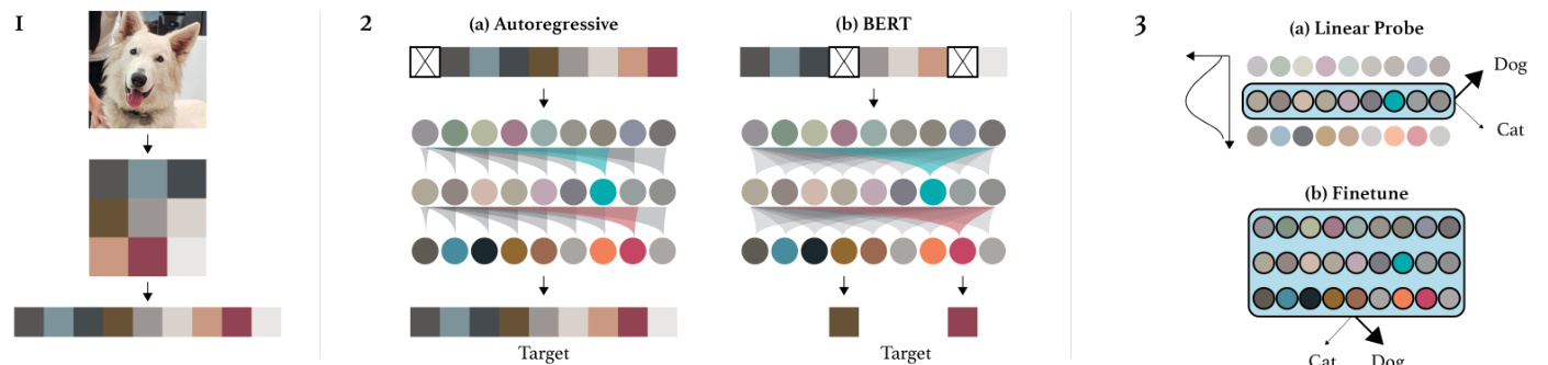
Figure 1. An overview of our approach. First, we pre-process raw images by resizing to a low resolution and reshaping into a 1D sequence. We then chose one of two pre-training objectives, auto-regressive next pixel prediction or masked pixel prediction. Finally, we evaluate the representations learned by these objectives with linear probes or fine-tuning.
图 1: 方法概述。首先,我们通过将原始图像调整为低分辨率并重塑为一维序列进行预处理。然后选择两种预训练目标之一:自回归的下一个像素预测或掩码像素预测。最后,通过线性探测或微调评估这些目标学习到的表征。
This is especially promising as our architecture uses a dense connectivity pattern which does not encode the 2D spatial structure of images yet is able to match and even outperform approaches which do. We report a set of experiments characterizing the performance of our approach on many datasets and in several different evaluation settings (low data, linear evaluation, full fine-tuning). We also conduct several experiments designed to better understand the achieved performance of these models. We investigate how representations are computed inside our model via the performance of linear probes as a function of model depth as well as studying how scaling the resolution and parameter count of the approach affects performance.
这尤其令人期待,因为我们的架构采用了密集连接模式,虽然未编码图像的二维空间结构,却能媲美甚至超越那些具备该结构的方法。我们通过一系列实验展示了该方法在多个数据集及不同评估场景(低数据量、线性评估、全微调)下的性能表现。同时,我们还进行了多项实验以深入理解这些模型的性能表现:通过线性探针分析表征在模型深度中的计算过程,并研究分辨率缩放和参数量对性能的影响。
2. Approach
2. 方法
Our approach consists of a pre-training stage followed by a fine-tuning stage. In pre-training, we explore both the auto-regressive and BERT objectives. We also apply the sequence Transformer architecture to predict pixels instead of language tokens.
我们的方法包括预训练阶段和微调阶段。在预训练中,我们同时探索了自回归目标和BERT目标。我们还应用了序列Transformer架构来预测像素而非语言token。
One way to measure representation quality is to fine-tune for image classification. Fine-tuning adds a small classification head to the model, used to optimize a classification objective and adapts all weights. Pre-training can be viewed as a favorable initialization or as a regularize r when used in combination with early stopping (Erhan et al., 2010).
衡量表征质量的一种方法是对图像分类进行微调。微调会在模型上添加一个小型分类头,用于优化分类目标并调整所有权重。预训练可视为有利的初始化方法,或与早停法 (early stopping) 结合使用时作为正则化手段 (Erhan et al., 2010)。
Another approach for measuring representation quality uses the pre-trained model as a feature extractor. In particular, given labeled examples $(X,Y)$ , the model is applied to $X$ to produce features $f_{X}$ . Then, a linear classifier is trained on $(f_{X},Y)$ . Linear probing captures the intuition that good features should linearly separate the classes of transfer tasks. Furthermore, linear probes help disentangle feature quality from model architecture: in fine-tuning, one model may outperform another because its architecture is more suited for the downstream task rather than because of better pretraining.
另一种衡量表征质量的方法是将预训练模型作为特征提取器使用。具体来说,给定标注样本$(X,Y)$,模型对$X$进行处理生成特征$f_{X}$,随后在$(f_{X},Y)$上训练线性分类器。线性探测(linear probing)体现了"优质特征应能线性分离迁移任务类别"的直观理念。此外,线性探测有助于区分特征质量与模型架构的影响:在微调过程中,某个模型的优势可能源于其架构更适配下游任务,而非预训练效果更优。
We begin this section by defining the auto-regressive and BERT objectives in the context of images. Next, we outline implementation details for our transformer decoder. Finally, we describe how the transformer is used for fine-tuning and how features are extracted for linear probes.
本节首先在图像背景下定义自回归( auto-regressive )和BERT目标。接着概述我们Transformer解码器的实现细节。最后描述如何将Transformer用于微调(fine-tuning)以及如何提取特征以进行线性探测(linear probes)。
2.1. Pre-training
2.1. 预训练
Given an unlabeled dataset $X$ consisting of high dimensional data $\boldsymbol{x}=(x_{1},...,x_{n})$ , we can pick a permutation $\pi$ of the set $[1,n]$ and model the density $p(x)$ auto-regressive ly as follows:
给定一个由高维数据 $\boldsymbol{x}=(x_{1},...,x_{n})$ 组成的无标签数据集 $X$,我们可以选择集合 $[1,n]$ 的一个排列 $\pi$,并以自回归方式对密度 $p(x)$ 建模如下:
$$
p(x)=\prod_{i=1}^{n}p(x_{\pi_{i}}|x_{\pi_{1}},...,x_{\pi_{i-1}},\theta)
$$
$$
p(x)=\prod_{i=1}^{n}p(x_{\pi_{i}}|x_{\pi_{1}},...,x_{\pi_{i-1}},\theta)
$$
When working with images, we pick the identity permutation $\pi_{i}=i$ for $1\leq i\leq n$ , also known as raster order. We train our model by minimizing the negative log-likelihood of the data:
在处理图像时,我们选择恒等排列 $\pi_{i}=i$ (其中 $1\leq i\leq n$),也称为光栅顺序。通过最小化数据的负对数似然来训练模型:
$$
L_{A R}=\underset{x\sim X}{\mathbb{E}}[-\log p(x)]
$$
$$
L_{A R}=\underset{x\sim X}{\mathbb{E}}[-\log p(x)]
$$
We also consider the BERT objective, which samples a sub-sequence $M\subset[1,n]$ such that each index $i$ independently has probability 0.15 of appearing in $M$ . We call $M$ the BERT mask, and we train our model by minimizing the negative log-likelihood of the “masked” elements $x_{M}$ conditioned on the “unmasked” ones $x_{[1,n]\setminus M}$ :
我们还考虑了BERT目标,它采样一个子序列$M\subset[1,n]$,使得每个索引$i$独立地有0.15的概率出现在$M$中。我们将$M$称为BERT掩码,并通过最小化以"未掩码"元素$x_{[1,n]\setminus M}$为条件的"掩码"元素$x_{M}$的负对数似然来训练模型:
$$
L_{B E R T}=\underset{x\sim X}{\mathbb{E}}\underset{M}{\mathbb{E}}\sum_{i\in M}\left[-\log p\left(x_{i}\vert x_{[1,n]\backslash M}\right)\right]
$$
$$
L_{B E R T}=\underset{x\sim X}{\mathbb{E}}\underset{M}{\mathbb{E}}\sum_{i\in M}\left[-\log p\left(x_{i}\vert x_{[1,n]\backslash M}\right)\right]
$$
In pre-training, we pick one of $L_{A R}$ or $L_{B E R T}$ and minimize the loss over our pre-training dataset.
在预训练阶段,我们选择 $L_{A R}$ 或 $L_{B E R T}$ 其中之一,并在预训练数据集上最小化损失。
2.2. Architecture
2.2. 架构
The transformer decoder takes an input sequence x1, ..., xn of discrete tokens and produces a $d$ -dimensional embedding for each position. The decoder is realized as a stack of $L$ blocks, the $l$ -th of which produces an intermediate embedding $h_{1}^{l},...,h_{n}^{l}$ also of dimension $d$ . We use the GPT-2 (Radford et al., 2019) formulation of the transformer decoder block, which acts on an input tensor $h^{l}$ as follows:
Transformer解码器接收一个由离散Token组成的输入序列x1, ..., xn,并为每个位置生成一个$d$维嵌入。该解码器由$L$个块堆叠而成,其中第$l$个块会生成维度同样为$d$的中间嵌入$h_{1}^{l},...,h_{n}^{l}$。我们采用GPT-2 (Radford et al., 2019)提出的Transformer解码器块结构,其作用于输入张量$h^{l}$的运算如下:
$$
\begin{array}{r}{n^{l}=\operatorname{layer_norm}(h^{l})\qquad}\ {a^{l}=h^{l}+\operatorname{multihead_attention}(n^{l})\qquad}\ {h^{l+1}=a^{l}+\operatorname*{mlp}(\operatorname{layer_norm}(a^{l}))\qquad}\end{array}
$$
$$
\begin{array}{r}{n^{l}=\operatorname{layer_norm}(h^{l})\qquad}\ {a^{l}=h^{l}+\operatorname{multihead_attention}(n^{l})\qquad}\ {h^{l+1}=a^{l}+\operatorname*{mlp}(\operatorname{layer_norm}(a^{l}))\qquad}\end{array}
$$
In particular, layer norms precede both the attention and mlp operations, and all operations lie strictly on residual paths. We find that such a formulation allows us to scale the transformer with ease.
具体来说,层归一化 (layer norm) 同时作用于注意力机制和前馈网络操作前,且所有操作严格位于残差路径上。我们发现这种结构能更轻松地扩展 Transformer 的规模。
The only mixing across sequence elements occurs in the attention operation, and to ensure proper conditioning when training the AR objective, we apply the standard upper triangular mask to the $n\times n$ matrix of attention logits. When using the BERT objective, no attention logit masking is required: after applying content embeddings to the input sequence, we zero out the positions in $M$ .
序列元素间唯一的混合发生在注意力操作中。为确保自回归(AR)目标训练时的正确条件约束,我们对 $n\times n$ 注意力对数矩阵应用标准的上三角掩码。当使用BERT目标时,则无需进行注意力对数掩码:在将内容嵌入应用到输入序列后,我们会将 $M$ 中的对应位置清零。
Additionally, since we learn independent position embeddings for each sequence element, our BERT model has no positional inductive biases (i.e. it is permutation invariant). Put another way, any spatial relationships between positions must be learned by the model at train time. This is not entirely true for the AR model, as choosing the raster order also fixes a pre specified ordering of the conditionals. Nevertheless, permutation invariance is a property in strong contrast to convolutional neural networks, which incorporate the inductive bias that features should arise from spatially proximate elements.
此外,由于我们为每个序列元素学习独立的位置嵌入 (position embeddings),我们的 BERT 模型不具备位置归纳偏置 (positional inductive biases)(即具有排列不变性)。换句话说,位置之间的任何空间关系都必须在训练时由模型自行学习。这对自回归 (AR) 模型并不完全成立,因为选择光栅顺序 (raster order) 同时也固定了条件概率的预设顺序。尽管如此,排列不变性与卷积神经网络 (convolutional neural networks) 形成鲜明对比,后者包含的归纳偏置要求特征应来自空间相邻的元素。
Following the final transformer layer, we apply a layer norm $n^{L}=\mathrm{layer}\mathrm{.norm}(h^{L})$ , and learn a projection from $n^{L}$ to logits parameter i zing the conditional distributions at each sequence element. When training BERT, we simply ignore the logits at unmasked positions.
在最终的Transformer层之后,我们应用了一层归一化 $n^{L}=\mathrm{layer}\mathrm{.norm}(h^{L})$ ,并学习从 $n^{L}$ 到logits的投影,用于参数化每个序列元素的条件分布。在训练BERT时,我们直接忽略未屏蔽位置的logits。
2.3. Fine-tuning
2.3. 微调
When fine-tuning, we average pool $n^{L}$ across the sequence dimension to extract a $d$ -dimensional vector of features per example:
微调时,我们在序列维度上对 $n^{L}$ 进行平均池化,以提取每个样本的 $d$ 维特征向量:
$$
f^{L}=\langle n_{i}^{L}\rangle_{i}
$$
$$
f^{L}=\langle n_{i}^{L}\rangle_{i}
$$
We learn a projection from $f^{L}$ to class logits, which we use to minimize a cross entropy loss $L_{C L F}$ .
我们学习从 $f^{L}$ 到类别逻辑值的投影,用于最小化交叉熵损失 $L_{C L F}$。
While fine-tuning on $L_{C L F}$ yields reasonable downstream performance, we find empirically that the joint objective
在对 $L_{CLF}$ 进行微调可获得合理的下游性能时,我们通过实验发现联合目标
$$
L_{G E N}+L_{C L F}
$$
$$
L_{G E N}+L_{C L F}
$$
$L_{G E N}\in{L_{A R},L_{B E R T}}$ works even better. Similar findings were reported by Radford et al. (2018).
$L_{G E N}\in{L_{A R},L_{B E R T}}$ 效果更佳。Radford等人 (2018) 也报告了类似发现。
2.4. Linear Probing
2.4. 线性探测 (Linear Probing)
Extracting fixed features for linear probing follows a similar procedure to fine-tuning, except that average pooling is not
提取固定特征用于线性探测的过程与微调类似,只是不进行平均池化
always at the final layer:
始终位于最终层:
$$
f^{l}=\langle n_{i}^{l}\rangle_{i}
$$
$$
f^{l}=\langle n_{i}^{l}\rangle_{i}
$$
where $0\le l\le L$ . We will show in the experiments section that the best features often lie in the middle of the network. As in fine-tuning, we project these intermediate features to produce class logits. Because we view the features as fixed when linear probing, this projection contains the only trainable weights, so we can only optimize $L_{C L F}$ .
其中 $0\le l\le L$。我们将在实验部分展示,最佳特征通常位于网络的中间层。与微调类似,我们将这些中间特征投影以生成类别逻辑值。由于在线性探测时我们将特征视为固定,该投影层包含唯一可训练的权重,因此我们只能优化 $L_{C L F}$。
3. Methodology
3. 方法论
Although supervised pre-training is the dominant paradigm for image classification, curating large labeled image datasets is both expensive and time consuming. Instead of further scaling up labeling efforts, we can instead aspire to learn general purpose representations from the much larger set of available unlabeled images and fine-tune them for classification. We investigate this setting using ImageNet as a proxy for a large unlabeled corpus, and small classic labeled datasets (CIFAR-10, CIFAR-100, STL-10) as proxies for downstream tasks. For our largest model, we use an additional 100 million unlabeled web images, filtered to be similar to ImageNet.
尽管监督式预训练是图像分类的主流范式,但构建大型标注图像数据集既昂贵又耗时。与其进一步扩大标注规模,我们更希望从更大量的未标注图像中学习通用表征,再针对分类任务进行微调。本研究以ImageNet作为大型未标注数据集的代理,并选用经典小型标注数据集(CIFAR-10、CIFAR-100、STL-10)作为下游任务代理。针对最大模型,我们还使用了经过筛选的1亿张与ImageNet相似的未标注网络图像。
Even in cases where labels are available, unsupervised or self-supervised pre-training can still provide benefits in data efficiency or on fine-tuning speed. We investigate this setting by pre-training without labels and then fine-tuning or linear probing with labels.
即使在有标签的情况下,无监督或自监督预训练仍能在数据效率或微调速度方面带来优势。我们通过无标签预训练、随后用标签进行微调或线性探测来研究这一场景。
3.1. Dataset and Data Augmentation
3.1. 数据集与数据增强
We use the ImageNet ILSVRC 2012 training dataset, splitting off $4%$ as our experimental validation set and report results on the ILSVRC 2012 validation set as our test set. For CIFAR-10, CIFAR-100 and STL-10, we split off $10%$ of the provided training set instead. We ignore the provided unlabeled examples in STL-10, which constitute a subset of ImageNet.
我们使用ImageNet ILSVRC 2012训练数据集,划分出$4%$作为实验验证集,并在ILSVRC 2012验证集上报告结果作为测试集。对于CIFAR-10、CIFAR-100和STL-10,我们从提供的训练集中划分出$10%$作为验证集。STL-10中提供的未标注样本(属于ImageNet子集)未被采用。
No data augmentation is used when pre-training on web images, and lightweight data augmentation is used when pre-training or fine-tuning on ImageNet. Specifically, when employing data augmentation, we randomly resize an image such that the shorter sidelength is in the range [256, 384] and then take a random $224\times224$ crop. When evaluating on ImageNet, we resize the image such that the shorter sidelength is 224, and use the single $224\times224$ center crop.
在网络图像上进行预训练时不使用数据增强,而在ImageNet上进行预训练或微调时采用轻量级数据增强。具体而言,使用数据增强时,我们会随机调整图像尺寸使短边长度处于[256, 384]范围内,然后随机裁剪出$224\times224$的区域。在ImageNet上评估时,将图像短边调整为224像素,并采用单一的$224\times224$中心裁剪。
When full-network fine-tuning on CIFAR-10 and CIFAR100, we use the augmentation popularized by Wide Residual Networks: 4 pixels are reflection padded on each side, and a $32\times32$ crop is randomly sampled from the padded image or its horizontal flip (Zagoruyko & Komodakis, 2016).
在CIFAR-10和CIFAR100上进行全网络微调时,我们采用了Wide Residual Networks推广的数据增强方法:每边进行4像素的反射填充,然后从填充后的图像或其水平翻转中随机采样一个$32\times32$的裁剪区域 (Zagoruyko & Komodakis, 2016)。
Once optimal hyper parameters are found, we fold our experimental validation set back into the training set, retrain the model, and report numbers on the respective test set.
找到最优超参数后,我们将实验验证集重新合并到训练集中,重新训练模型,并在相应测试集上报告结果。
3.2. Context Reduction
3.2. 上下文缩减
Because the memory requirements of the transformer decoder scale quadratically with context length when using dense attention, we must employ further techniques to reduce context length. If we naively trained a transformer on a sequence of length $224^{2}\times3$ , our attention logits would be tens of thousands of times larger than those used in language models and even a single layer would not fit on a GPU. To deal with this, we first resize our image to a lower resolution, which we call the input resolution (IR). Our models have IRs of either $32^{2}\times3$ , $48^{2}\times3$ , or $64^{2}\times3$ .
由于Transformer解码器在使用密集注意力机制时,其内存需求会随上下文长度呈平方级增长,我们必须采用更多技术来缩短上下文长度。若直接在 $224^{2}\times3$ 长度的序列上训练Transformer,其注意力对数将比语言模型所用的大数万倍,甚至单层网络也无法放入GPU内存。为此,我们首先将图像降采样至较低分辨率(称为输入分辨率(IR)),模型采用的IR包括 $32^{2}\times3$ 、 $48^{2}\times3$ 或 $64^{2}\times3$ 三种规格。
An IR of $32^{2}\times3$ is still quite computationally intensive. While working at even lower resolutions is tempting, prior work has demonstrated human performance on image classification begins to drop rapidly below this size (Torralba et al., 2008). Instead, motivated by early color display palettes, we create our own 9-bit color palette by clustering (R, G, B) pixel values using $k$ -means with $k=512$ . Using this palette yields an input sequence length 3 times shorter than the standard (R, G, B) palette, while still encoding color faithfully. A similar approach was applied to spatial patches by Ranzato et al. (2014). We call the resulting context length ( $32^{2}$ or $48^{2}$ or $64^{2}$ ) the model resolution (MR). Note that this reduction breaks permutation invariance of the color channels, but keeps the model spatially invariant.
$32^{2}\times3$ 的输入分辨率 (IR) 在计算上仍然相当密集。虽然使用更低分辨率很诱人,但先前研究表明图像分类任务中的人类表现会在此尺寸以下快速下降 (Torralba et al., 2008)。受早期彩色显示调色板启发,我们通过 $k$ -均值聚类 ($k=512$) 创建了自定义的9位色彩调色板。该调色板使输入序列长度比标准 (R, G, B) 调色板缩短3倍,同时保持色彩保真度。Ranzato et al. (2014) 曾在空间补丁上应用过类似方法。我们将最终上下文长度 ($32^{2}$ 或 $48^{2}$ 或 $64^{2}$) 称为模型分辨率 (MR)。需注意这种压缩会破坏色彩通道的排列不变性,但保持模型的空间不变性。
3.3. Model
3.3. 模型
Our largest model, iGPT-XL, contains $L=60$ layers and uses an embedding size of $d=3072$ for a total of 6.8B parameters. Our next largest model, iGPT-L, is essentially identical to GPT-2 with $L~=~48$ layers, but contains a slightly smaller embedding size of $d=1536$ (vs 1600) for a total of 1.4M parameters. We use the same model code as GPT-2, except that we initialize weights in the layerdependent fashion as in Sparse Transformer (Child et al., 2019) and zero-initialize all projections producing logits.
我们最大的模型iGPT-XL包含$L=60$层,嵌入维度为$d=3072$,总参数量达68亿。次大的iGPT-L模型结构与GPT-2基本一致($L~=~48$层),但采用略小的嵌入维度$d=1536$(原为1600),总参数量14亿。我们沿用GPT-2的模型代码,仅作两点调整:(1) 采用Sparse Transformer (Child et al., 2019)提出的分层权重初始化方法;(2) 对生成logits的所有投影层进行零初始化。
We also train iGPT-M, a $455\mathrm{M}$ parameter model with $L=$ 36 and $d=1024$ and iGPT-S, a 76M parameter model with $L=24$ and $d=512$ to study the effect of model capacity on representation quality in a generative model.
我们还训练了iGPT-M(一个4.55亿参数模型,$L=36$,$d=1024$)和iGPT-S(一个7600万参数模型,$L=24$,$d=512$),以研究生成式模型中模型容量对表征质量的影响。
3.4. Training
3.4. 训练
When pre-training iGPT-XL, we use a batch size of 64 and train for 2M iterations, and for all other models we use a batch size of 128 and train for 1M iterations. We use Adam with $\beta_{1}=0.9$ and $\beta_{2}=0.95$ and sequentially try the learning rates 0.01, 0.003, 0.001, 0.0003, ..., stopping once the final validation loss starts increasing. The learning rate is warmed up for one epoch, and then decays to 0 following a cosine schedule. No dropout is used.
在预训练iGPT-XL时,我们使用64的批次大小并训练200万次迭代,其他所有模型则使用128的批次大小并训练100万次迭代。我们采用Adam优化器,设置$\beta_{1}=0.9$和$\beta_{2}=0.95$,并依次尝试0.01、0.003、0.001、0.0003等学习率,当最终验证损失开始上升时停止。学习率经过一个周期的预热后,按余弦调度衰减至0。未使用dropout。
When fine-tuning, we use the same batch size and Adam hyper parameters. Here, we do not employ a cosine schedule, and early stop once we reach the maximum validation accuracy. Again, no dropout is used.
微调时,我们使用相同的批次大小和Adam超参数。此处未采用余弦调度,一旦达到最大验证准确率即提前停止。同样未使用dropout。
When running a linear probe on ImageNet, we follow recent literature and use SGD with momentum 0.9 and a high learning rate (we try the values 30, 10, 3, ... in the manner described above) (He et al., 2019). We train for 1000000 iterations with a cosine learning rate schedule. Finally, when running a linear probe on CIFAR-10, CIFAR-100, or STL10, we use the L-BFGS algorithm for consistency with prior results (Pedregosa et al., 2011).
在ImageNet上运行线性探测时,我们遵循近期文献方法,采用动量0.9的SGD优化器,并设置较高学习率(按上述方式尝试30、10、3等值)(He et al., 2019)。训练采用余弦学习率调度,共进行100万次迭代。最后,在CIFAR-10、CIFAR-100或STL10数据集上运行线性探测时,为保持与先前研究结果的一致性,我们使用L-BFGS算法(Pedregosa et al., 2011)。
4. Experiments and Results
4. 实验与结果
We begin with experiments and results from the autoregressive formulation of iGPT. Comparisons with the BERT formulation appear in Section 4.6.
我们首先从iGPT的自回归(autoregressive)公式的实验和结果开始。与BERT公式的比较见第4.6节。
4.1. What Representation Works Best in a Generative Model Without Latent Variables?
4.1. 无潜在变量生成模型的最佳表示方式是什么?
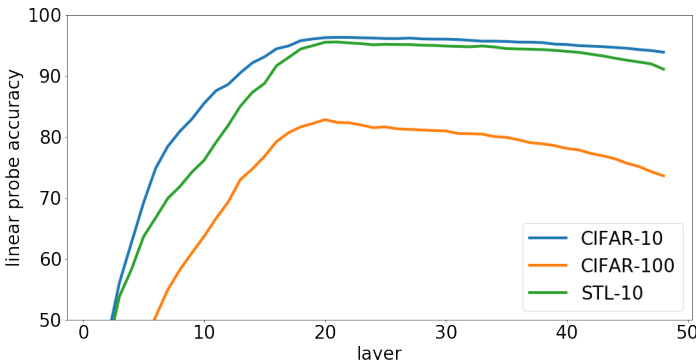
Figure 2. Representation quality depends on the layer from which we extract features. In contrast with supervised models, the best representations for these generative models lie in the middle of the network. We plot this unimodal dependence on depth by showing linear probes for iGPT-L on CIFAR-10, CIFAR-100, and STL-10.
图 2: 表征质量取决于提取特征的网络层级。与监督模型不同,这些生成模型的最佳表征位于网络中间层。我们通过展示iGPT-L在CIFAR-10、CIFAR-100和STL-10上的线性探针结果,绘制了这种随深度变化的单峰依赖关系。
In supervised pre-training, representation quality tends to increase monotonically with depth, such that the best represent at ions lie at the penultimate layer (Zeiler & Fergus, 2014). Indeed, since a linear layer produces class logits from pre-logits, a good classifier necessarily achieves high accuracy on a linear probe of its pre-logits. If a downstream task also involves classification, it is empirically validated that penultimate features perform well.
在监督式预训练中,表征质量往往随深度单调递增,最佳表征通常位于倒数第二层 (Zeiler & Fergus, 2014) 。实际上,由于线性层通过预对数生成类别逻辑值,优质分类器必然能在其预对数的线性探测中实现高准确率。当下游任务同样涉及分类时,经验表明倒数第二层特征表现优异。
With generative pre-training, it is not obvious whether a task like pixel prediction is relevant to image classification. This suggests that the penultimate layer of a model trained for pixel prediction might not produce the most useful representations for classification. Latent variable models such as VAEs can avoid this issue by explicitly learning a representation of the input data, but deep auto regressive generative models have the same width and connectivity pattern at every layer. Our first experiment studies how representation quality varies over one set of candidate representations: different layers of a generative model. We observe a very different behavior from supervised learning: representations first improve as a function of depth, and then, starting around the middle layer, begin to deteriorate until the penultimate layer (Figure 2).
通过生成式预训练,像像素预测这样的任务是否与图像分类相关并不明显。这表明,为像素预测训练的模型的倒数第二层可能不会产生对分类最有用的表征。变分自编码器 (VAE) 等潜在变量模型可以通过显式学习输入数据的表征来避免这个问题,但深度自回归生成模型在每一层都具有相同的宽度和连接模式。我们的第一个实验研究了表征质量如何在一组候选表征中变化:生成模型的不同层。我们观察到与监督学习截然不同的行为:表征质量首先随着深度增加而提升,然后从中层开始逐渐恶化,直到倒数第二层 (图 2)。
This behavior potentially suggests that these generative models operate in two phases. In the first phase, each position gathers information from its surrounding context in order to build a more global image representation. In the second phase, this contextual i zed input is used to solve the conditional next pixel prediction task. This could resemble the behavior of encoder-decoder architectures common across deep learning, but learned within a monolithic architecture via a pre-training objective.
这一行为可能表明,这些生成模型分两个阶段运行。第一阶段,每个位置从周围上下文中收集信息,以构建更全局的图像表征。第二阶段,这些经过上下文处理的输入被用于解决条件性下一像素预测任务。这可能类似于深度学习常见的编码器-解码器架构行为,但通过预训练目标在单一架构中学习完成。
Consequently, when evaluating a generative model with a linear probe, it is important to search for the best layer. Taking the final layer on CIFAR-10 decreases performance by $2.4%$ , the difference between a baseline and a state-ofthe-art result. In all settings, we find that the dependence of representation quality on depth is strongly unimodal.
因此,在使用线性探针评估生成模型时,寻找最佳层至关重要。在CIFAR-10数据集上直接选用最后一层会使性能下降$2.4%$,这一差距相当于基线结果与最先进成果之间的差异。在所有实验设置中,我们发现表征质量对网络深度的依赖呈现明显的单峰分布特征。
4.2. Better Generative Models Learn Better Representations
4.2. 更优的生成式模型 (Generative Models) 学习更优的表征
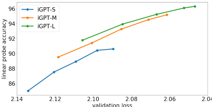
Figure 3. Plot of representation quality as a function of validation generative loss. Each line tracks a model throughout generative pre-training: the dotted markers denote checkpoints at steps 65K, 131K, 262K, 524K, and 1000K. The positive slope suggests a link between improved generative performance and improved representation quality. Larger models produce better representations than smaller ones both at the end of training and at the same value of validation loss. iGPT-XL is not shown since it was trained on a different dataset.
图 3: 表征质量随验证生成损失变化的曲线图。每条线代表一个模型在生成式预训练过程中的表现:虚线标记对应65K、131K、262K、524K和1000K训练步数的检查点。正斜率表明生成性能提升与表征质量改善存在关联。无论训练结束时还是相同验证损失值下,较大模型始终比较小模型产生更优表征。iGPT-XL因使用不同训练数据集而未显示。
Using the linear probe as a tool for measuring representation quality, we investigate whether better generative models (as measured by log-prob on held-out data) also learn better representations.
我们使用线性探针作为衡量表征质量的工具,研究生成模型(以保留数据对数概率为衡量标准)是否在学习过程中获得了更好的表征。
In Figure 3, we see that as validation loss on the autoregressive objective decreases throughout training, linear probe accuracy increases as well. This trend holds across several model capacities, with higher capacity models achieving better validation losses. This highlights the importance of scale for our approach. Note that for a given validation loss value, bigger models also perform better.
在图3中,我们看到随着自回归目标验证损失在整个训练过程中降低,线性探针准确率也相应提升。这一趋势在不同模型容量下均成立,容量更高的模型能获得更优的验证损失。这凸显了规模对本方法的重要性。值得注意的是,在给定验证损失值的情况下,更大模型的性能也更优。
Table 1. Comparing linear probe accuracies between our models and state-of-the-art models utilizing unsupervised ImageNet transfer or supervised ImageNet transfer.
| Model | Acc | Unsup Transfer | Sup Transfer |
| CIFAR-10 | |||
| ResNet-152 | 94 | ||
| SimCLR | 95.3 | ||
| iGPT-L | 96.3 | ||
| CIFAR-100 | |||
| ResNet-152 | 78.0 | ||
| SimCLR | 80.2 | ||
| iGPT-L | 82.8 | ||
| STL-10 | |||
| AMDIM-L | 94.2 | ||
| iGPT-L | 95.5 |
表 1: 我们的模型与利用无监督ImageNet迁移或有监督ImageNet迁移的先进模型之间的线性探测准确率对比。
| 模型 | 准确率 | 无监督迁移 | 有监督迁移 |
|---|---|---|---|
| CIFAR-10 | |||
| ResNet-152 | 94 | √ | |
| SimCLR | 95.3 | √ | |
| iGPT-L | 96.3 | √ | |
| CIFAR-100 | |||
| ResNet-152 | 78.0 | √ | |
| SimCLR | 80.2 | √ | |
| iGPT-L | 82.8 | √ | |
| STL-10 | |||
| AMDIM-L | 94.2 | √ | |
| iGPT-L | 95.5 | √ |
4.3. Linear Probes on CIFAR and STL-10
4.3. CIFAR 和 STL-10 上的线性探针
In addition to CIFAR-10, we also evaluate linear probes on CIFAR-100 and STL-10 (Figure 2) to check whether the learned representations are useful across multiple datasets. For this evaluation setting, we achieve state-of-the-art across the entire spectrum of pre-training approaches (Table 1). For example, on CIFAR-10, our model achieves $96.3%$ , outperforming both SimCLR (pre-trained on ImageNet without labels) and a ResNet-152 (pre-trained on ImageNet with labels). In fact, on all three datasets a linear classifier fit to the representations of iGPT-L outperforms the end-to-end supervised training of a WideResNet baseline.
除了 CIFAR-10,我们还在 CIFAR-100 和 STL-10 (图 2) 上评估线性探针,以检验所学表征是否适用于多个数据集。在此评估设置中,我们在所有预训练方法中均取得了最先进的性能 (表 1)。例如,在 CIFAR-10 上,我们的模型达到了 $96.3%$,优于 SimCLR (在无标签 ImageNet 上预训练) 和 ResNet-152 (在有标签 ImageNet 上预训练)。事实上,在所有三个数据集上,基于 iGPT-L 表征训练的线性分类器都优于 WideResNet 基线的端到端监督训练。
Note that our model is trained at the same input resolution (IR) as CIFAR, whereas models trained at the standard ImageNet IR may experience distribution shock upon linear evaluation. As a counterpoint, though STL-10 has an IR of $96^{2}\times3$ , we still outperform AMDIM-L when we downsample to $32^{2}\times3$ before linear probing. We also note that fine-tuning should allow models trained at high IR to adjust to low resolution input.
需要注意的是,我们的模型采用与CIFAR相同的输入分辨率(IR)进行训练,而以标准ImageNet分辨率训练的模型在进行线性评估时可能会遭遇分布偏移。作为对比,虽然STL-10的输入分辨率为$96^{2}\times3$,但当我们在线性探测前将其下采样至$32^{2}\times3$时,性能仍优于AMDIM-L。此外需要指出,通过微调可以使高分辨率训练的模型适应低分辨率输入。
4.4. Linear Probes on ImageNet
4.4. ImageNet 上的线性探针
Recently, there has been a resurgence of interest in unsupervised and self-supervised learning on ImageNet, evaluated using linear probes on ImageNet. This is a particularly difficult setting for us, since we cannot efficiently train at the standard ImageNet input resolution (IR). Indeed, when training iGPT-L with a model resolution (MR) of $32^{2}$ , we achieve only $60.3%$ best-layer linear probe accuracy. As with CIFAR-10, scale is critical to our approach: iGPT
近来,ImageNet上的无监督和自监督学习重新引发关注,其评估方式是在ImageNet上使用线性探针。这对我们而言是个特别困难的设定,因为无法在标准ImageNet输入分辨率(IR)下高效训练。事实上,当以$32^{2}$的模型分辨率(MR)训练iGPT-L时,我们仅获得$60.3%$的最佳层线性探针准确率。与CIFAR-10类似,规模对我们的方法至关重要:iGPT
Table 2. Comparing linear probe accuracies between our models and state-of-the-art self-supervised models. A blank input resolution (IR) corresponds to a model working at standard ImageNet resolution. We report the best performing configuration for each contrastive method, finding that our models achieve comparable performance.
| Method | IR | Params (M) | Features | Acc |
| Rotation | orig. | 86 | 8192 | 55.4 |
| iGPT-L | 322.3 | 1362 | 1536 | 60.3 |
| BigBiGAN | orig. | 86 | 8192 | 61.3 |
| iGPT-L | 482.3 | 1362 | 1536 | 65.2 |
| AMDIM | orig. | 626 | 8192 | 68.1 |
| MoCo | orig. | 375 | 8192 | 68.6 |
| iGPT-XL | 642.3 | 6801 | 3072 | 68.7 |
| SimCLR | orig. | 24 | 2048 | 69.3 |
| CPCv2 | orig. | 303 | 8192 | 71.5 |
| iGPT-XL | 642.3 | 6801 | 15360 | 72.0 |
| SimCLR | orig. | 375 | 8192 | 76.5 |
表 2: 对比我们的模型与最先进的自监督模型之间的线性探测准确率。空白输入分辨率 (IR) 表示模型在标准 ImageNet 分辨率下工作。我们报告了每种对比方法的最佳性能配置,发现我们的模型实现了可比的性能。
| 方法 | IR | 参数量 (M) | 特征维度 | 准确率 |
|---|---|---|---|---|
| Rotation | orig. | 86 | 8192 | 55.4 |
| iGPT-L | 322.3 | 1362 | 1536 | 60.3 |
| BigBiGAN | orig. | 86 | 8192 | 61.3 |
| iGPT-L | 482.3 | 1362 | 1536 | 65.2 |
| AMDIM | orig. | 626 | 8192 | 68.1 |
| MoCo | orig. | 375 | 8192 | 68.6 |
| iGPT-XL | 642.3 | 6801 | 3072 | 68.7 |
| SimCLR | orig. | 24 | 2048 | 69.3 |
| CPCv2 | orig. | 303 | 8192 | 71.5 |
| iGPT-XL | 642.3 | 6801 | 15360 | 72.0 |
| SimCLR | orig. | 375 | 8192 | 76.5 |
M achieves $54.5%$ accuracy and iGPT-S achieves $41.9%$ accuracy.
M 达到了 54.5% 的准确率,iGPT-S 达到了 41.9% 的准确率。
The first obvious optimization is to increase MR while staying within accelerator memory limits. With a MR of $48^{2}$ , iGPT-L achieves a best-layer accuracy of $65.2%$ using 1536 features and with a MR of $64^{2}$ , iGPT-XL achieves a bestlayer accuracy of $68.7%$ using 3072 features.
第一个明显的优化是在加速器内存限制内提高MR (Memory Resolution)。当MR为$48^{2}$时,iGPT-L使用1536个特征实现了65.2%的最佳层准确率;当MR为$64^{2}$时,iGPT-XL使用3072个特征实现了68.7%的最佳层准确率。
Since contrastive methods report their best results on 8192 features, we would ideally evaluate iGPT with an embedding dimension 8192 for comparison. Training such a model is prohibitively expensive, so we instead concatenate features from multiple layers as an approximation. However, our features tend to be correlated across layers, so we need more of them to be competitive. If we concatenate features from 5 layers centered at the best single layer of iGPT-XL, we achieve an accuracy of $72.0%$ using 15360 features, which is competitive with recent contrastive learning approaches (Table 2). Note that we require more parameters and compute to achieve this accuracy, but we work at low resolution and without utilizing knowledge of the 2D input structure.
由于对比方法在8192个特征上报告了最佳结果,我们理想情况下应使用嵌入维度为8192的iGPT进行评估以便比较。训练这样的模型成本过高,因此我们改为通过拼接多层特征作为近似方案。然而,我们的特征在层间往往存在相关性,因此需要更多特征才能保持竞争力。若以iGPT-XL最佳单层为中心拼接5层特征,使用15360个特征时准确率达到$72.0%$,这与近期对比学习方法的表现相当(表2)。需要注意的是,我们为实现该准确率需要更多参数和计算量,但我们的工作在低分辨率下进行,且未利用2D输入结构的先验知识。
4.5. Full Fine-tuning
4.5. 全参数微调
To achieve even higher accuracy on downstream tasks, we adapt the entire model for classification through fine-tuning. Building off of the previous analysis, we tried attaching the classification head to the layer with the best representations. Though this setup trains faster than one with the head attached at the end, the latter is able to leverage greater model depth and eventually outperforms.
为了在下游任务中获得更高的准确率,我们通过微调使整个模型适应分类任务。基于之前的分析,我们尝试将分类头附加到具有最佳表征的层。虽然这种设置比将分类头附加在末端的方案训练速度更快,但后者能够利用更大的模型深度,最终表现更优。
On CIFAR-10, iGPT-L achieves $99.0%$ accuracy and on CIFAR-100, it achieves $88.5%$ accuracy after fine-tuning. We outperform Auto Augment, the best supervised model on these datasets, though we do not use sophisticated data augmentation techniques. In fact, $99.0%$ ties GPipe, the best model which pre-trains using ImageNet labels.
在CIFAR-10数据集上,iGPT-L经过微调后达到了99.0%的准确率,在CIFAR-100数据集上达到88.5%的准确率。尽管未使用复杂的数据增强技术,我们的表现仍优于这些数据集上最佳的监督模型Auto Augment。事实上,99.0%的准确率与使用ImageNet标签预训练的最佳模型GPipe持平。
Table 3. Comparing fine-tuning performance between our models and state-of-the-art models utilizing supervised ImageNet transfer. We also include Auto Augment, the best performing model trained end-to-end on CIFAR. Table results: Auto Augment (Cubuk et al., 2019), SimCLR (Chen et al., 2020), GPipe (Huang et al., 2019), Eff i cent Net (Tan & Le, 2019)
| Model | Acc | Unsup Transfer | Sup Transfer |
| CIFAR-10 | |||
| AutoAugment | 98.5 | ||
| SimCLR | 98.6 | ||
| GPipe | 99.0 | ||
| iGPT-L | 99.0 | ||
| CIFAR-100 | |||
| iGPT-L | 88.5 | ||
| SimCLR | 89.0 | ||
| AutoAugment | 89.3 | ||
| EfficientNet | 91.7 |
表 3: 我们的模型与利用监督式 ImageNet 迁移的先进模型在微调性能上的对比。我们还纳入了 Auto Augment (Cubuk 等人, 2019) ,这是在 CIFAR 上端到端训练表现最佳的模型。表格结果来源: Auto Augment (Cubuk 等人, 2019), SimCLR (Chen 等人, 2020), GPipe (Huang 等人, 2019), EfficientNet (Tan & Le, 2019)
| 模型 | 准确率 | 无监督迁移 | 监督迁移 |
|---|---|---|---|
| CIFAR-10 | |||
| AutoAugment | 98.5 | ||
| SimCLR | 98.6 | √ | |
| GPipe | 99.0 | √ | |
| iGPT-L | 99.0 | √ | |
| CIFAR-100 | |||
| iGPT-L | 88.5 | √ | |
| SimCLR | 89.0 | √ | |
| AutoAugment | 89.3 | ||
| EfficientNet | 91.7 | √ |
On ImageNet, we achieve $66.3%$ accuracy after fine-tuning at MR $32^{2}$ , a bump of $6%$ over linear probing. When finetuning at MR $48^{2}$ , we achieve $72.6%$ accuracy, with a similar $7%$ bump over linear probing. However, our models still slightly under perform Isometric Neural Nets (Sandler et al., 2019), which achieves $70.2%$ at an IR of $28^{2}\times3$ .
在ImageNet上,我们在MR $32^{2}$ 微调后达到了66.3%的准确率,比线性探测高出6%。当在MR $48^{2}$ 进行微调时,准确率达到72.6%,同样比线性探测高出约7%。不过,我们的模型表现仍略逊于等距神经网络 (Isometric Neural Nets) (Sandler et al., 2019),后者在IR $28^{2}\times3$ 下达到了70.2%的准确率。
Finally, as a baseline for ImageNet fine-tuning, we train the classification objective from a random initialization. At MR $48^{2}$ , a model with tuned learning rate and dropout achieves $53.2%$ after 18 epochs, $19.4%$ worse than the pretrained model. Comparatively, the pre-trained model is much quicker to fine-tune, achieving the same $53.2%$ loss in roughly a single epoch.
最后,作为ImageNet微调的基线,我们从随机初始化开始训练分类目标。在MR $48^{2}$下,经过学习率和dropout调整的模型在18个epoch后达到$53.2%$,比预训练模型低$19.4%$。相比之下,预训练模型的微调速度要快得多,仅需约1个epoch就能达到相同的$53.2%$损失。
When fine-tuning, it is important to search over learning rates again, as the optimal learning rate on the joint training objective is often an order of magnitude smaller than that for pre-training. We also tried regularizing with dropout, though we did not observe any clear benefits. It is easy to overfit the classification objective on small datasets, so we employ early stopping based on validation accuracy.
微调时,必须重新搜索学习率,因为联合训练目标的最优学习率通常比预训练时小一个数量级。我们还尝试了使用dropout进行正则化,但未观察到明显收益。小数据集上分类目标容易过拟合,因此我们采用基于验证准确率的早停策略。
4.6. BERT
4.6. BERT
Given the success of BERT in language, we train iGPT-L at an input resolution of $32^{2}\times3$ and a model resolution of $32^{2}$ (Figure 4). On CIFAR-10, we observe that linear probe accuracy at every layer is worse than that of the autoregressive model, with best-layer performance more than $1%$ lower. Best-layer accuracy on ImageNet is $6%$ lower.
鉴于BERT在语言领域的成功,我们在输入分辨率为$32^{2}\times3$、模型分辨率为$32^{2}$的条件下训练了iGPT-L (图4)。在CIFAR-10数据集上,我们发现每一层的线性探测准确率都低于自回归模型,最佳层性能低了超过1%。在ImageNet上的最佳层准确率则低了6%。
However, during fine-tuning, BERT makes up much of this gap. A fully fine-tuned CIFAR-10 model achieves $98.6%$ accuracy, only $0.4%$ behind its auto-regressive counterpart, while a fully fine-tuned ImageNet model achieves $66.5%$ , slightly surpassing auto-regressive performance.
然而,在微调过程中,BERT大幅缩小了这一差距。经过完整微调的CIFAR-10模型达到了98.6%的准确率,仅比自回归模型低0.4%;而完整微调的ImageNet模型则达到66.5%的准确率,略微超越了自回归模型的性能。

Figure 4. Comparison of auto-regressive pre-training with BERT pre-training using iGPT-L at an input resolution of $32^{2}\times3$ . Blue bars display linear probe accuracy and orange bars display finetune accuracy. Bold colors show the performance boost from ensembling BERT masks. We see that auto-regressive models produce much better features than BERT models after pre-training, but BERT models catch up after fine-tuning.
图 4: 使用iGPT-L在输入分辨率为$32^{2}\times3$时,自回归预训练与BERT预训练的比较。蓝色柱状图显示线性探测准确率,橙色柱状图显示微调准确率。加粗颜色表示通过集成BERT掩码带来的性能提升。可以看出,预训练后自回归模型产生的特征远优于BERT模型,但经过微调后BERT模型能追平表现。
Finally, because inputs to the BERT model are masked at training time, we must also mask them at evaluation time to keep inputs in-distribution. This masking corruption may hinder the BERT model’s ability to correctly predict image classes. Therefore, we also try an evaluation scheme where we sample 5 independent masks for each input and take the modal prediction, breaking ties at random. In this setting, CIFAR-10 results are largely unchanged, but on ImageNet, we gain almost $1%$ on our linear probes and fine-tunes.
最后,由于BERT模型的输入在训练时会被掩码处理,在评估时我们也必须对输入进行掩码以保持分布一致性。这种掩码干扰可能会影响BERT模型正确预测图像分类的能力。因此,我们还尝试了一种评估方案:为每个输入采样5个独立掩码,取众数预测结果(随机处理平局情况)。在此设置下,CIFAR-10的结果基本保持不变,但在ImageNet上,我们的线性探测和微调性能提升了近$1%$。
4.7. Low-Data CIFAR-10 Classification
4.7. 低数据量 CIFAR-10 分类
Evaluations of unsupervised representations often reuse supervised learning datasets which have thousands to millions of labeled examples. However, a representation which has robustly encoded a semantic concept should be exceedingly data efficient. As inspiration, we note that humans are able to reliably recognize even novel concepts with a single example (Carey and Bartlett 1978). This motivates evaluating performance in a low-data regime as well. It is also a more realistic evaluation setting for the potential practical usefulness of an approach since it better matches the common real-world scenario of an abundance of raw data but a lack of labels.
对无监督表征的评估通常复用监督学习数据集,这些数据集包含数千到数百万带标签样本。然而,一个稳健编码语义概念的表征应当具备极高的数据效率。受人类仅需单样本就能可靠识别新概念的能力启发 (Carey and Bartlett 1978) ,我们同时采用低数据量环境下的性能评估。这种设定更能反映实际应用场景——原始数据丰富但标签稀缺,因此对方法潜在实用价值的评估也更具现实意义。
In contrast with recent approaches for low-data classification, we do not make use of pseudo-labeling or data aug- mentation. Instead, we work directly on a subset of the raw supervised dataset, extracting features using our pre-trained model, and training a linear classifier on those features.
与近期低数据分类方法不同,我们既不采用伪标签技术也不使用数据增强手段。而是直接处理原始监督数据集的子集:通过预训练模型提取特征,并基于这些特征训练线性分类器。
Table 4. Comparing performance on low-data CIFAR-10. By leveraging many unlabeled ImageNet images, iGPT-L is able to outperform methods such as Mean Teacher (Tarvainen & Valpola, 2017) and MixMatch (Berthelot et al., 2019) but still under performs the state of the art methods (Xie et al., 2019; Sohn et al., 2020). Our approach to semi-supervised learning is very simple since we only fit a logistic regression classifier on iGPT-L’s features without any data augmentation or fine-tuning - a significant difference from specially designed semi-supervised approaches. Other results reported from FixMatch (Sohn et al., 2020).
表 4: 低数据量 CIFAR-10 上的性能对比。通过利用大量未标注的 ImageNet 图像,iGPT-L 能够超越 Mean Teacher (Tarvainen & Valpola, 2017) 和 MixMatch (Berthelot et al., 2019) 等方法,但仍逊色于最先进方法 (Xie et al., 2019; Sohn et al., 2020)。我们的半监督学习方法非常简单,因为只需在 iGPT-L 的特征上拟合逻辑回归分类器,无需任何数据增强或微调——这与专门设计的半监督方法存在显著差异。其他结果来自 FixMatch (Sohn et al., 2020)。
| Model | 40labels | 2501abels | 4000labels |
| MeanTeacher | 32.3±2.3 | 9.2±0.2 | |
| MixMatch | 47.5±11.5 | 11.0±0.9 | 6.4 ± 0.1 |
| iGPT-L | 26.8 ±1.5 | 12.4±0.6 | 5.7 ± 0.1 |
| UDA | 29.0 ±5.9 | 8.8 ± 1.1 | 4.9 ± 0.2 |
| FixMatchRA | 13.8±3.4 | 5.1 ± 0.7 | 4.3 ± 0.1 |
| FixMatchCTA | 11.4±3.4 | 5.1±0.3 | 4.3±0.2 |
| 模型 | 40标签 | 2501标签 | 4000标签 |
|---|---|---|---|
| MeanTeacher | 32.3±2.3 | 9.2±0.2 | |
| MixMatch | 47.5±11.5 | 11.0±0.9 | 6.4±0.1 |
| iGPT-L | 26.8±1.5 | 12.4±0.6 | 5.7±0.1 |
| UDA | 29.0±5.9 | 8.8±1.1 | 4.9±0.2 |
| FixMatchRA | 13.8±3.4 | 5.1±0.7 | 4.3±0.1 |
| FixMatchCTA | 11.4±3.4 | 5.1±0.3 | 4.3±0.2 |
As is standard in the low-data setting, we sample 5 random subsets and report mean and standard deviation accuracies (Table 4). On CIFAR-10, we find that with 4 labels per class, we achieve $73.2%$ accuracy outperforming MixMatch with much lower variance between runs and with 25 labels per class, we achieve $87.6%$ accuracy, though still significantly lower than the state of the art, FixMatch.
按照低数据设置的标准做法,我们随机抽取5个子集并报告准确率的均值与标准差(表4)。在CIFAR-10数据集上,当每类4个标注样本时,我们取得了73.2%的准确率,优于MixMatch方法且实验间方差显著降低;当每类25个标注样本时,准确率达到87.6%,但仍显著低于当前最优方法FixMatch。
Although we have established that large models are necessary for producing good representations, large models are also difficult to fine-tune in the ultra-low data regime. Indeed, we find that iGPT-L quickly memorizes a 40-example training set and fails to generalize well, achieving only $42.1%$ accuracy. We expect adapting recent approaches to semi-supervised learning will help in this setting.
尽管我们已经证实大模型对于生成优质表征是必要的,但在极低数据量场景下对大模型进行微调仍存在困难。实验发现,iGPT-L模型在仅40个样本的训练集上会迅速过拟合,泛化性能较差,准确率仅为$42.1%$。我们预期采用半监督学习(semi-supervised learning)的最新方法将有助于改善这一状况。
5. Related Work
5. 相关工作
Many generative models have been developed and evaluated for their representation learning capabilities. Notably, GANs (Goodfellow et al., 2014; Radford et al., 2015; Don- ahue et al., 2016) and VAEs (Kingma & Welling, 2013; Kingma et al., 2014; Higgins et al., 2017) have been wellstudied.
许多生成模型已被开发并评估其表征学习能力。值得注意的是,GAN (Goodfellow et al., 2014; Radford et al., 2015; Donahue et al., 2016) 和 VAE (Kingma & Welling, 2013; Kingma et al., 2014; Higgins et al., 2017) 已得到深入研究。
As of yet, most generative model based approaches have not been competitive with supervised and self-supervised methods in the image domain. A notable exception is BigBiGAN (Donahue & Simonyan, 2019) which first demonstrated that sufficiently high fidelity generative models learn image representations which are competitive with other selfsupervised methods.
目前,大多数基于生成式模型的方法在图像领域仍无法与监督学习和自监督方法相抗衡。一个显著的例外是BigBiGAN (Donahue & Simonyan, 2019),它首次证明高保真度的生成式模型能够学习到与其他自监督方法相媲美的图像表征。
Many self-supervised approaches focus on designing auxiliary objectives which support the learning of useful represent at ions without attempting to directly model the input data. Examples include surrogate classification (Dosovitskiy et al., 2015), jigsaw puzzle solving (Noroozi & Favaro, 2016), and rotation prediction (Gidaris et al., 2018). A cluster of similar approaches based on contrastive losses comparing various views and transformations of input images have recently driven significant progress in self-supervised learning (Hjelm et al., 2018; Bachman et al., 2019; Tian et al., 2019).
许多自监督方法专注于设计辅助目标函数,这些目标函数支持学习有用的表征而不直接建模输入数据。例如代理分类 (Dosovitskiy et al., 2015) 、拼图求解 (Noroozi & Favaro, 2016) 和旋转预测 (Gidaris et al., 2018) 。最近,一系列基于对比损失的相似方法通过比较输入图像的不同视角和变换,在自监督学习领域取得了显著进展 (Hjelm et al., 2018; Bachman et al., 2019; Tian et al., 2019) 。
Among contrastive approaches, our work is most similar to Contrast Predictive Coding (Oord et al., 2018) which also utilizes a auto regressive prediction objective, but in a learned latent space, and to Selfie (Trinh et al., 2019) which trains a bidirectional self-attention architecture on top of a standard convolutional network to differentiate correct vs wrong patches.
在对比方法中,我们的工作与对比预测编码 (Contrastive Predictive Coding) [Oord et al., 2018] 最为相似,后者同样采用自回归预测目标,但作用于学习到的潜在空间;也与 Selfie [Trinh et al., 2019] 类似,该方法在标准卷积网络之上训练双向自注意力架构以区分正确与错误的图像块。
Our work is directly inspired by the success of generative pre-training methods developed for Natural Language Processing. These methods predict some parts of a piece of text conditioned on other parts. Our work explores two training objectives in this framework, auto regressive prediction as originally explored for modern neural sequence models by Dai & Le (2015), and a denoising objective, similar to BERT (Devlin et al., 2018). The context in-painting approach of Pathak et al. (2016) also explores pre-training by predicting corruptions but predicts large regions of high-resolution images.
我们的工作直接受到自然语言处理领域生成式预训练方法成功的启发。这些方法基于文本片段的部分内容预测其他部分。在此框架下,我们探索了两种训练目标:Dai & Le (2015) 为现代神经序列模型首次提出的自回归预测目标,以及类似 BERT (Devlin et al., 2018) 的去噪目标。Pathak et al. (2016) 提出的上下文修复方法同样通过预测损坏内容进行预训练,但针对的是高分辨率图像的大区域预测。
Kolesnikov et al. (2019); Goyal et al. (2019) conducted rigorous investigations of existing self-supervised methods. Several of our findings are consistent with their results, including the benefits of scale and the non-monotonic performance of representations with depth in certain architectures.
Kolesnikov等人 (2019) 和Goyal等人 (2019) 对现有自监督方法进行了严谨研究。我们的多项发现与其结论一致,包括规模化优势以及特定架构中表征性能随深度呈现非单调变化。
Expressive auto regressive models tractably optimizing likelihood were first applied to images by Uria et al. (2013) and popularized by Oord et al. (2016) serving for the basis of several papers similarly adapting transformers to the problem of generative image modeling (Parmar et al., 2018; Child et al., 2019).
Uria等人(2013)首次将可优化似然函数的自回归表达模型应用于图像领域,随后Oord等人(2016)的研究使其得到普及,为多篇论文将Transformer应用于生成式图像建模问题奠定了基础(Parmar等人,2018;Child等人,2019)。
Ke et al. (2018) introduced the pixel-by-pixel CIFAR10 task and first benchmarked the performance of a 1D sequence transformer on a competitive image classification dataset. Rives et al. (2019) similarly investigates whether the recent success of unsupervised pre-training in NLP applies to other domains, observing promising results on protein sequence data.
Ke等人 (2018) 提出了逐像素CIFAR10任务,首次在具有竞争力的图像分类数据集上对一维序列Transformer的性能进行了基准测试。Rives等人 (2019) 同样研究了无监督预训练在自然语言处理领域的最新成功是否适用于其他领域,并在蛋白质序列数据上观察到了有希望的结果。
6. Discussion and Conclusion
6. 讨论与结论
Our results suggest that generative image modeling continues to be a promising route to learn high-quality unsupervised image representations. Simply predicting pixels learns state of the art representations for low resolution datasets. In high resolution settings, our approach is also competitive with other self-supervised results on ImageNet.
我们的研究结果表明,生成式图像建模 (Generative Image Modeling) 仍然是学习高质量无监督图像表征的有效途径。仅通过像素预测就能在低分辨率数据集上学习到最先进的表征。在高分辨率场景下,我们的方法在ImageNet上也与其他自监督学习成果具有竞争力。
However, our experiments also demonstrate several areas for improvement. We currently model low resolution inputs with self-attention. By comparison, most other selfsupervised results use CNN based encoders that easily work with high resolution images. It is not immediately obvious how to best bridge the gap between performant autoregressive and disc rim i native models. Additionally, we observed that our approach requires large models in order to learn high quality representations. iGPT-L has 2 to 3 times as many parameters as similarly performing models on ImageNet and uses more compute.
然而,我们的实验也揭示了若干待改进之处。当前我们采用自注意力机制处理低分辨率输入,而多数其他自监督研究成果使用基于CNN的编码器,这类方法能轻松处理高分辨率图像。如何最佳弥合高性能自回归模型与判别模型之间的差距,目前尚无明确方案。此外,我们发现该方法需要大型模型才能学习高质量表征——iGPT-L的参数规模是ImageNet上性能相近模型的2至3倍,且计算消耗更大。
Although dense self-attention was a deliberate choice for this work due to it being domain agnostic and widely used in NLP, it becomes very memory and computationally expensive due to its quadratic scaling with sequence length. We mitigated this via the context reduction techniques discussed in section 3.2 but it is still a significant limitation. Future work could instead address this via architectural changes by exploring more efficient self-attention approaches. Several promising techniques have recently been developed such as local 2D relative attention (Bello et al., 2019; Ramachandran et al., 2019), sparse attention patterns (Child et al., 2019), locality sensitive hashing (Kitaev et al., 2020), and multiscale modeling (Menick & Kal ch brenner, 2018).
尽管密集自注意力 (self-attention) 因其领域无关性及在 NLP 中的广泛应用而被本研究采用,但其随序列长度呈二次方增长的特性会显著增加内存和计算开销。我们通过第 3.2 节讨论的上下文缩减技术缓解了这一问题,但这仍是重要限制。未来工作可通过架构改进探索更高效的自注意力方法,例如局部二维相对注意力 (Bello et al., 2019; Ramachandran et al., 2019)、稀疏注意力模式 (Child et al., 2019)、局部敏感哈希 (Kitaev et al., 2020) 和多尺度建模 (Menick & Kalchbrenner, 2018) 等近期涌现的有前景技术。
Finally, our results, considered together with Donahue & Simonyan (2019), suggest revisiting the representation learning capabilities of other families of generative models such as flows (Dinh et al., 2014; Kingma & Dhariwal, 2018) and VAEs in order to study whether they show similarly competitive representation learning capabilities.
最后,结合Donahue & Simonyan (2019)的研究,我们的结果表明有必要重新审视其他生成模型族(如流模型(flow)(Dinh et al., 2014; Kingma & Dhariwal, 2018)和变分自编码器(VAE)的表征学习能力,以探究它们是否展现出同样具有竞争力的表征学习性能。
References
参考文献
Radford, A., Metz, L., and Chintala, S. Unsupervised represent ation learning with deep convolutional generative adversarial networks. arXiv preprint arXiv:1511.06434, 2015.
Radford, A., Metz, L., 和 Chintala, S. 基于深度卷积生成对抗网络的无监督表示学习. arXiv预印本 arXiv:1511.06434, 2015.
Radford, A., Narasimhan, K., Salimans, T., and Sutskever, I. Improving language understanding by generative pretraining. 2018.
Radford, A., Narasimhan, K., Salimans, T., and Sutskever, I. 通过生成式预训练提升语言理解能力。2018.
Radford, A., Wu, J., Child, R., Luan, D., Amodei, D., and Sutskever, I. Language models are unsupervised multitask learners. 2019.
Radford, A., Wu, J., Child, R., Luan, D., Amodei, D., and Sutskever, I. 语言模型是无监督多任务学习器。2019。
Rama chandra n, P., Parmar, N., Vaswani, A., Bello, I., Lev- skaya, A., and Shlens, J. Stand-alone self-attention in vision models. arXiv preprint arXiv:1906.05909, 2019.
Rama chandra n, P., Parmar, N., Vaswani, A., Bello, I., Lev- skaya, A., and Shlens, J. 视觉模型中的独立自注意力机制. arXiv preprint arXiv:1906.05909, 2019.
Ranzato, M., Szlam, A., Bruna, J., Mathieu, M., Collobert, R., and Chopra, S. Video (language) modeling: a baseline for generative models of natural videos. arXiv preprint arXiv:1412.6604, 2014.
Ranzato, M., Szlam, A., Bruna, J., Mathieu, M., Collobert, R., and Chopra, S. 视频(语言)建模: 自然视频生成模型的基础研究. arXiv preprint arXiv:1412.6604, 2014.
Rives, A., Goyal, S., Meier, J., Guo, D., Ott, M., Zitnick, C. L., Ma, J., and Fergus, R. Biological structure and function emerge from scaling unsupervised learning to 250 million protein sequences. bioRxiv, pp. 622803, 2019.
Rives, A., Goyal, S., Meier, J., Guo, D., Ott, M., Zitnick, C. L., Ma, J., and Fergus, R. 通过将无监督学习扩展到2.5亿个蛋白质序列实现生物结构与功能的涌现。bioRxiv, pp. 622803, 2019.
Sandler, M., Baccash, J., Zhmoginov, A., and Howard, A. Non-disc rim i native data or weak model? on the relative importance of data and model resolution. In Proceedings of the IEEE International Conference on Computer Vision Workshops, pp. 0–0, 2019.
Sandler, M., Baccash, J., Zhmoginov, A., and Howard, A. 非歧视性数据还是弱模型?论数据与模型分辨率的相对重要性。见《IEEE国际计算机视觉研讨会论文集》,第0-0页,2019年。
Sohn, K., Berthelot, D., Li, C.-L., Zhang, Z., Carlini, N., Cubuk, E. D., Kurakin, A., Zhang, H., and Raffel, C. Fixmatch: Simplifying semi-supervised learning with consistency and confidence. arXiv preprint arXiv:2001.07685, 2020.
Sohn, K., Berthelot, D., Li, C.-L., Zhang, Z., Carlini, N., Cubuk, E. D., Kurakin, A., Zhang, H., and Raffel, C. Fixmatch: 通过一致性和置信度简化半监督学习。arXiv preprint arXiv:2001.07685, 2020.
Tan, M. and Le, Q. V. Efficient net: Rethinking model scaling for convolutional neural networks. arXiv preprint arXiv:1905.11946, 2019.
Tan, M. 和 Le, Q. V. EfficientNet: 重新思考卷积神经网络(CNN)的模型缩放。arXiv预印本 arXiv:1905.11946, 2019.
Tarvainen, A. and Valpola, H. Mean teachers are better role models: Weight-averaged consistency targets improve semi-supervised deep learning results. In Advances in neural information processing systems, pp. 1195–1204, 2017.
Tarvainen, A. 和 Valpola, H. 均值教师是更好的榜样:权重平均一致性目标提升半监督深度学习效果。载于《神经信息处理系统进展》,第1195-1204页,2017年。
Tian, Y., Krishnan, D., and Isola, P. Contrastive multiview coding. arXiv preprint arXiv:1906.05849, 2019.
Tian, Y., Krishnan, D., 和 Isola, P. 对比多视图编码. arXiv预印本 arXiv:1906.05849, 2019.
Torralba, A., Fergus, R., and Freeman, W. T. 80 million tiny images: A large data set for non parametric object and scene recognition. IEEE transactions on pattern analysis and machine intelligence, 30(11):1958–1970, 2008.
Torralba, A., Fergus, R., and Freeman, W. T. 八千万微小图像:用于非参数化物体与场景识别的大规模数据集。IEEE transactions on pattern analysis and machine intelligence, 30(11):1958–1970, 2008.
A. Experimental details
A. 实验细节
A.1. Hyper parameters
A.1. 超参数
In Table 5, we present the learning rates used to train each model in the paper. When using too high a learning rate, we observe an irrecoverable loss spike early on in training. Conversely, with too low a learning rate, training is stable but loss improves slowly and eventually under performs. As we increase model size, the irrecoverable loss spike occurs at even lower learning rates. This motivates our procedure of sequentially searching learning rates from large to small and explains why larger models use lower learning rates than smaller models at fixed input resolution.
表5中,我们列出了论文中训练每个模型所使用的学习率。当学习率过高时,我们观察到训练初期会出现不可恢复的损失骤增;反之,学习率过低则训练稳定但损失下降缓慢,最终导致性能欠佳。随着模型规模增大,不可恢复的损失骤增现象会在更低学习率下出现。这促使我们采用从大到小逐步搜索学习率的策略,也解释了为何在固定输入分辨率下,较大模型比较小模型使用更低学习率。
We used an Adam $\beta_{2}$ of 0.95 instead of the default 0.999 because the latter causes loss spikes during training. We did not use weight decay because applying a small weight decay of 0.01 did not change representation quality.
我们使用了Adam优化器中$\beta_{2}$为0.95的参数(而非默认值0.999),因为后者会导致训练过程中出现损失值尖峰。未采用权重衰减(weight decay)技术,因为施加0.01的小权重衰减并未改变表征质量。
On iGPT-S, we found small gains in representation quality from using float32 instead of float16, from untying the token embedding matrix and the matrix producing token logits, and from zero initializing the matrices producing token and class logits. We applied these settings to all models.
在iGPT-S上,我们发现使用float32而非float16、解绑token嵌入矩阵与生成token逻辑值的矩阵、以及对生成token和类别逻辑值的矩阵进行零初始化,都能小幅提升表征质量。我们将这些设置应用于所有模型。
When training BERT models, one additional hyper parameter is the masking probability, set to $15%$ in Devlin et al. (2018).
在训练BERT模型时,一个额外的超参数是掩码概率(masking probability),在Devlin等人(2018)的研究中设置为$15%$。
Table 5. Learning rates used for each model, objective, and input resolution (IR) combination.
| Model | Objective | IR | Learning Rate |
| iGPT-S | auto-regressive | 322×3 | 0.003 |
| iGPT-M | auto-regressive | 322 × 3 | 0.003 |
| iGPT-L | auto-regressive | 322 × 3 | 0.001 |
| iGPT-L | auto-regressive | 482 × 3 | 0.01 |
| iGPT-XL | auto-regressive | 64² × 3 | 0.0003 |
| iGPT-S | BERT | 322× 3 | 0.01 |
| iGPT-M | BERT | 322 × 3 | 0.003 |
| iGPT-L | BERT | 322×3 | 0.001 |
表 5: 各模型、训练目标和输入分辨率 (IR) 组合使用的学习率。
| 模型 | 训练目标 | IR | 学习率 |
|---|---|---|---|
| iGPT-S | 自回归 (auto-regressive) | 322×3 | 0.003 |
| iGPT-M | 自回归 (auto-regressive) | 322×3 | 0.003 |
| iGPT-L | 自回归 (auto-regressive) | 322×3 | 0.001 |
| iGPT-L | 自回归 (auto-regressive) | 482×3 | 0.01 |
| iGPT-XL | 自回归 (auto-regressive) | 64²×3 | 0.0003 |
| iGPT-S | BERT | 322×3 | 0.01 |
| iGPT-M | BERT | 322×3 | 0.003 |
| iGPT-L | BERT | 322×3 | 0.001 |
We also tried higher masking rates of $20%$ , $25%$ , $30%$ , and $35%$ , finding that $20%$ matched the performance of $15%$ , though higher probabilities decreased performance.
我们还尝试了更高的掩码率,分别为 $20%$、$25%$、$30%$ 和 $35%$,发现 $20%$ 的表现与 $15%$ 相当,但更高的概率会降低性能。