Big Bird: Transformers for Longer Sequences
Big Bird: 更长序列的Transformer
Abstract
摘要
Transformers-based models, such as BERT, have been one of the most successful deep learning models for NLP. Unfortunately, one of their core limitations is the quadratic dependency (mainly in terms of memory) on the sequence length due to their full attention mechanism. To remedy this, we propose, BIGBIRD, a sparse attention mechanism that reduces this quadratic dependency to linear. We show that BIGBIRD is a universal approx im at or of sequence functions and is Turing complete, thereby preserving these properties of the quadratic, full attention model. Along the way, our theoretical analysis reveals some of the benefits of having $O(1)$ global tokens (such as CLS), that attend to the entire sequence as part of the sparse attention mechanism. The proposed sparse attention can handle sequences of length up to 8x of what was previously possible using similar hardware. As a consequence of the capability to handle longer context, BIGBIRD drastically improves performance on various NLP tasks such as question answering and sum mari z ation. We also propose novel applications to genomics data.
基于Transformer的模型(如BERT)已成为自然语言处理(NLP)领域最成功的深度学习模型之一。然而,由于其全注意力机制,这类模型存在一个核心限制:对序列长度的二次方依赖(主要体现在内存消耗上)。为解决这一问题,我们提出了BIGBIRD——一种将二次方依赖降为线性关系的稀疏注意力机制。我们证明BIGBIRD是序列函数的通用逼近器,具备图灵完备性,从而保留了全注意力模型的这些特性。理论分析揭示了稀疏注意力机制中设置$O(1)$全局token(如CLS)的优势,这些token能够关注整个序列。该稀疏注意力机制可处理的序列长度达到原有硬件条件下最大长度的8倍。得益于处理长上下文的能力,BIGBIRD在问答和摘要等NLP任务上显著提升了性能。我们还提出了其在基因组数据中的创新应用。
1 Introduction
1 引言
Models based on Transformers [91], such as BERT [22, 63], are wildly successful for a wide variety of Natural Language Processing (NLP) tasks and consequently are mainstay of modern NLP research. Their versatility and robustness are the primary drivers behind the wide-scale adoption of Transformers. The model is easily adapted for a diverse range of sequence based tasks – as a seq2seq model for translation [91], sum mari z ation [66], generation [15], etc. or as a standalone encoders for sentiment analysis [83], POS tagging [65], machine reading comprehension [93], etc. – and it is known to vastly outperform previous sequence models like LSTM [37]. The key innovation in Transformers is the introduction of a self-attention mechanism, which can be evaluated in parallel for each token of the input sequence, eliminating the sequential dependency in recurrent neural networks, like LSTM. This parallelism enables Transformers to leverage the full power of modern SIMD hardware accelerators like GPUs/TPUs, thereby facilitating training of NLP models on datasets of unprecedented size. This ability to train on large scale data has led to surfacing of models like BERT [22] and T5 [75], which pretrain transformers on large general purpose corpora and transfer the knowledge to down-stream task. The pre training has led to significant improvement in low data regime downstream tasks [51] as well as tasks with sufficient data [101] and thus have been a major force behind the ubiquity of transformers in contemporary NLP.
基于Transformer [91]的模型,如BERT [22, 63],在各种自然语言处理(NLP)任务中取得了巨大成功,因此成为现代NLP研究的主流。其多功能性和鲁棒性是Transformer被广泛采用的主要原因。该模型能轻松适配多种基于序列的任务——作为seq2seq模型用于翻译[91]、摘要生成[66]、文本生成[15]等任务,或作为独立编码器用于情感分析[83]、词性标注[65]、机器阅读理解[93]等任务——且已知其性能远超LSTM [37]等传统序列模型。Transformer的核心创新是自注意力(self-attention)机制,该机制可并行计算输入序列中每个token的关联权重,消除了LSTM等循环神经网络的时序依赖性。这种并行性使Transformer能充分利用GPU/TPU等现代SIMD硬件加速器,从而支持前所未有的大规模NLP模型训练。这种大规模训练能力催生了BERT [22]和T5 [75]等模型,它们先在通用语料库上预训练Transformer,再将知识迁移至下游任务。预训练技术显著提升了小数据量下游任务[51]和充足数据任务[101]的性能,成为当前NLP领域普遍采用Transformer的重要推动力。
The self-attention mechanism overcomes constraints of RNNs (namely the sequential nature of RNN) by allowing each token in the input sequence to attend independently to every other token in the sequence. This design choice has several interesting repercussions. In particular, the full self-attention have computational and memory requirement that is quadratic in the sequence length. We note that while the corpus can be large, the sequence length, which provides the context in many applications is very limited. Using commonly available current hardware and model sizes, this requirement translates to roughly being able to handle input sequences of length 512 tokens. This reduces its direct applicability to tasks that require larger context, like QA [60], document classification, etc.
自注意力机制通过允许输入序列中的每个token独立关注序列中的其他所有token,克服了RNN的局限性(即RNN的顺序性)。这一设计选择带来了一些有趣的影响。特别是,完整的自注意力在计算和内存需求上与序列长度呈平方关系。我们注意到,虽然语料库可能很大,但在许多应用中提供上下文的序列长度非常有限。使用当前常见的硬件和模型规模,这一需求大致转化为能够处理512个token长度的输入序列。这限制了其直接适用于需要更大上下文的任务,如问答[60]、文档分类等。
However, while we know that self-attention and Transformers are useful, our theoretical understanding is rudimentary. What aspects of the self-attention model are necessary for its performance? What can we say about the expressivity of Transformers and similar models? Apriori, it was not even clear from the design if the proposed self-attention mechanism was as effective as RNNs. For example, the self-attention does not even obey sequence order as it is permutation e qui variant. This concern has been partially resolved, as Yun et al. [104] showed that transformers are expressive enough to capture all continuous sequence to sequence functions with a compact domain. Meanwhile, Pérez et al. [72] showed that the full transformer is Turing Complete (i.e. can simulate a full Turing machine). Two natural questions arise: Can we achieve the empirical benefits of a fully quadratic self-attention scheme using fewer inner-products? Do these sparse attention mechanisms preserve the expressivity and flexibility of the original network?
然而,尽管我们知道自注意力机制和Transformer模型很有用,但对其理论理解仍处于初级阶段。自注意力模型的哪些方面对其性能至关重要?关于Transformer及其类似模型的表现力,我们能得出什么结论?从设计上看,最初甚至无法确定所提出的自注意力机制是否与循环神经网络(RNN)同样有效。例如,自注意力机制并不遵循序列顺序,因为它具有排列等变性。这一担忧已得到部分解决,因为Yun等人[104]证明Transformer具有足够强的表现力,能够捕捉定义在紧致域上的所有连续序列到序列函数。同时,Pérez等人[72]表明完整版的Transformer具备图灵完备性(即能模拟完整的图灵机)。由此衍生出两个自然问题:能否通过更少的内积运算实现完全二次自注意力方案的经验优势?这些稀疏注意力机制是否能保持原始网络的表现力和灵活性?
In this paper, we address both the above questions and produce a sparse attention mechanism that improves performance on a multitude of tasks that require long contexts. We systematically develop BIGBIRD, an attention mechanism whose complexity is linear in the number of tokens (Sec. 2). We take inspiration from graph spars if i cation methods and understand where the proof for expressiveness of Transformers breaks down when full-attention is relaxed to form the proposed attention pattern. This understanding helped us develop BIGBIRD, which is theoretically as expressive and also empirically useful. In particular, our BIGBIRD consists of three main part:
在本文中,我们同时解决了上述两个问题,并提出了一种稀疏注意力机制,该机制在需要长上下文的多项任务中提升了性能。我们系统性地开发了BIGBIRD,这是一种注意力机制,其复杂度与token数量呈线性关系(见第2节)。我们从图稀疏化方法中汲取灵感,并理解了当将全注意力放宽以形成所提出的注意力模式时,Transformer表达能力的证明在何处失效。这一理解帮助我们开发了BIGBIRD,该机制在理论上具有同等表达能力,并在实践中也表现出实用性。具体而言,我们的BIGBIRD包含三个主要部分:
This leads to a high performing attention mechanism scaling to much longer sequence lengths (8x).
这使得注意力机制的性能得到提升,能够扩展到更长的序列长度(8倍)。
To summarize, our main contributions are:
总结来说,我们的主要贡献包括:
1.1 Related Work
1.1 相关工作
There have been a number of interesting attempts, that were aimed at alleviating the quadratic dependency of Transformers, which can broadly categorized into two directions. First line of work embraces the length limitation and develops method around it. Simplest methods in this category just employ sliding window [93], but in general most work fits in the following general paradigm: using some other mechanism select a smaller subset of relevant contexts to feed in the transformer and optionally iterate, i.e. call transformer block multiple time with different contexts each time. Most prominently, SpanBERT [42], ORQA [54], REALM [34], RAG [57] have achieved strong performance for different tasks. However, it is worth noting that these methods often require significant engineering efforts (like back prop through large scale nearest neighbor search) and are hard to train.
为缓解Transformer的二次方依赖问题,已有许多有趣的尝试,这些方法可大致分为两个方向。第一种思路接受长度限制并围绕其开发方法。此类中最简单的方法仅采用滑动窗口[93],但大多数工作遵循以下通用范式:通过其他机制选择较小的相关上下文子集输入Transformer,并可选择迭代(即每次用不同上下文多次调用Transformer模块)。其中最突出的SpanBERT[42]、ORQA[54]、REALM[34]和RAG[57]在不同任务中取得了强劲性能。但值得注意的是,这些方法通常需要大量工程努力(如通过大规模最近邻搜索进行反向传播)且训练难度较高。
Second line of work questions if full attention is essential and have tried to come up with approaches that do not require full attention, thereby reducing the memory and computation requirements. Prominently, Dai et al. [21], Sukhbaatar et al. [82], Rae et al. [74] have proposed auto-regresive models that work well for left-to-right language modeling but suffer in tasks which require bidirectional context. Child et al. [16] proposed a sparse model that reduces the complexity to $O(n{\sqrt{n}})$ , Kitaev et al. [49] further reduced the complexity to $O(n\log(n))$ by using LSH to compute nearest neighbors.
第二条研究方向质疑全注意力机制的必要性,并尝试提出无需全注意力的方法以降低内存和计算需求。其中,Dai等人[21]、Sukhbaatar等人[82]、Rae等人[74]提出的自回归模型在从左到右的语言建模中表现良好,但在需要双向上下文的任务中存在局限。Child等人[16]提出稀疏模型将复杂度降至$O(n{\sqrt{n}})$,Kitaev等人[49]则通过局部敏感哈希(LSH)计算最近邻将复杂度进一步降至$O(n\log(n))$。

Figure 1: Building blocks of the attention mechanism used in BIGBIRD. White color indicates absence of attention. (a) random attention with $r=2$ , (b) sliding window attention with $w=3$ (c) global attention with $g=2$ . (d) the combined BIGBIRD model.
图 1: BIGBIRD中使用的注意力机制构建模块。白色表示无注意力。(a) 随机注意力(r=2),(b) 滑动窗口注意力(w=3),(c) 全局注意力(g=2),(d) 组合后的BIGBIRD模型。
Ye et al. [103] proposed binary partitions of the data where as Qiu et al. [73] reduced complexity by using block sparsity. Recently, Longformer [8] introduced a localized sliding window based mask with few global mask to reduce computation and extended BERT to longer sequence based tasks. Finally, our work is closely related to and built on the work of Extended Transformers Construction [4]. This work was designed to encode structure in text for transformers. The idea of global tokens was used extensively by them to achieve their goals. Our theoretical work can be seen as providing a justification for the success of these models as well. It is important to note that most of the aforementioned methods are heuristic based and empirically are not as versatile and robust as the original transformer, i.e. the same architecture do not attain SoTA on multiple standard benchmarks. (There is one exception of Longformer which we include in all our comparisons, see App. E.3 for a more detailed comparison). Moreover, these approximations do not come with theoretical guarantees.
Ye等人[103]提出了数据的二元划分方法,而Qiu等人[73]则通过使用块稀疏性来降低复杂度。最近,Longformer[8]引入了一种基于局部滑动窗口的掩码机制,辅以少量全局掩码,以减少计算量,并将BERT扩展到更长序列的任务中。最后,我们的工作与Extended Transformers Construction[4]密切相关,并在此基础上构建。该工作旨在为Transformer编码文本结构,他们广泛使用了全局token的概念来实现目标。我们的理论研究也可以视为对这些模型成功的一种理论支撑。值得注意的是,上述大多数方法都是基于启发式的,经验上不如原始Transformer那样通用和鲁棒,即同一架构无法在多个标准基准测试中达到最优水平(Longformer是个例外,我们将其纳入所有比较中,详见附录E.3的详细对比)。此外,这些近似方法缺乏理论保证。
2 BIGBIRD Architecture
2 BIGBIRD 架构
In this section, we describe the BIGBIRD model using the generalised attention mechanism that is used in each layer of transformer operating on an input sequence ${\pmb X}=({\pmb x}_ {1},...,{\pmb x}_{n})\in\mathbb{R}^{n\times d}$ The generalized attention mechanism is described by a directed graph $D$ whose vertex set is $[n]=$ ${1,\ldots,n}$ . The set of arcs (directed edges) represent the set of inner products that the attention mechanism will consider. Let $N(i)$ denote the out-neighbors set of node $i$ in $D$ , then the $i^{\mathrm{th}}$ output vector of the generalized attention mechanism is defined as
在本节中,我们使用广义注意力机制来描述BIGBIRD模型,该机制作用于输入序列 ${\pmb X}=({\pmb x}_ {1},...,{\pmb x}_{n})\in\mathbb{R}^{n\times d}$ 的每一层Transformer。广义注意力机制通过一个有向图 $D$ 来描述,其顶点集为 $[n]=$ ${1,\ldots,n}$。弧集(有向边)表示注意力机制将考虑的内积集合。设 $N(i)$ 表示节点 $i$ 在 $D$ 中的出邻居集,则广义注意力机制的第 $i^{\mathrm{th}}$ 个输出向量定义为
$$
\operatorname{ArfN}_ {D}(X)_ {i}={\pmb x}_ {i}+\sum_{h=1}^{H}\sigma\left(Q_{h}({\pmb x}_ {i})K_{h}({\pmb X}_ {N(i)})^{T}\right)\cdot V_{h}({\pmb X}_{N(i)})
$$
$$
\operatorname{ArfN}_ {D}(X)_ {i}={\pmb x}_ {i}+\sum_{h=1}^{H}\sigma\left(Q_{h}({\pmb x}_ {i})K_{h}({\pmb X}_ {N(i)})^{T}\right)\cdot V_{h}({\pmb X}_{N(i)})
$$
where $Q_{h},K_{h}:\mathbb{R}^{d}\rightarrow\mathbb{R}^{m}$ are query and key functions respectively, $V_{h}:\mathbb{R}^{d}\rightarrow\mathbb{R}^{d}$ is a value function, $\sigma$ is a scoring function (e.g. softmax or hardmax) and $H$ denotes the number of heads. Also note $X_{N(i)}$ corresponds to the matrix formed by only stacking ${\pmb{x}_{j}:j\in N(i)}$ and not all the inputs. If $D$ is the complete digraph, we recover the full quadratic attention mechanism of Vaswani et al. [91]. To simplify our exposition, we will operate on the adjacency matrix $A$ of the graph $D$ even though the underlying graph maybe sparse. To elaborate, $\dot{A}\in[0,\dot{1}]^{n\times n}$ with $A(i,j)=1$ if query $i$ attends to key $j$ and is zero otherwise. For example, when $A$ is the ones matrix (as in BERT), it leads to quadratic complexity, since all tokens attend on every other token. This view of self-attention as a fully connected graph allows us to exploit existing graph theory to help reduce its complexity. The problem of reducing the quadratic complexity of self-attention can now be seen as a graph spars if i cation problem. It is well-known that random graphs are expanders and can approximate complete graphs in a number of different contexts including in their spectral properties [80, 38]. We believe sparse random graph for attention mechanism should have two desiderata: small average path length between nodes and a notion of locality, each of which we discuss below.
其中 $Q_{h},K_{h}:\mathbb{R}^{d}\rightarrow\mathbb{R}^{m}$ 分别是查询 (query) 和键 (key) 函数,$V_{h}:\mathbb{R}^{d}\rightarrow\mathbb{R}^{d}$ 是值 (value) 函数,$\sigma$ 是评分函数(如 softmax 或 hardmax),$H$ 表示头数。注意 $X_{N(i)}$ 对应仅由 ${\pmb{x}_{j}:j\in N(i)}$ 堆叠而成的矩阵,而非全部输入。若 $D$ 为完整有向图,则恢复 Vaswani 等人 [91] 的完全二次注意力机制。为简化表述,我们将基于图 $D$ 的邻接矩阵 $A$ 进行操作(即使底层图可能是稀疏的)。具体而言,$\dot{A}\in[0,\dot{1}]^{n\times n}$ 满足 $A(i,j)=1$(当查询 $i$ 关注键 $j$ 时)否则为零。例如,当 $A$ 为全1矩阵(如 BERT)时,由于所有 token 都相互关注,会导致二次复杂度。将自注意力视为全连接图的视角,使我们能利用现有图论来降低其复杂度。降低自注意力二次复杂度的问题可视为图稀疏化问题。众所周知,随机图具有扩展性,能在包括谱特性在内的多种情境中近似完全图 [80, 38]。我们认为注意力机制的稀疏随机图应具备两个特性:节点间较短的平均路径长度和局部性概念,下文将分别讨论。
Let us consider the simplest random graph construction, known as Erd6s-Rényi model, where each edge is independently chosen with a fixed probability. In such a random graph with just $\tilde{\Theta}(n)$ edges, the shortest path between any two nodes is logarithmic in the number of nodes [17, 43]. As a consequence, such a random graph approximates the complete graph spectrally and its second eigenvalue (of the adjacency matrix) is quite far from the first eigenvalue [9, 10, 6]. This property leads to a rapid mixing time for random walks in the grpah, which informally suggests that information can flow fast between any pair of nodes. Thus, we propose a sparse attention where each query attends over $r$ random number of keys i.e. $A(i,\cdot)=1$ for $r$ randomly chosen keys (see Fig. 1a).
让我们考虑最简单的随机图构建方法,即Erd6s-Rényi模型,其中每条边都以固定概率独立选择。在这种仅有$\tilde{\Theta}(n)$条边的随机图中,任意两个节点之间的最短路径与节点数量呈对数关系[17, 43]。因此,这种随机图在谱意义上近似于完全图,其邻接矩阵的第二特征值与第一特征值相差较大[9, 10, 6]。这一特性使得图中随机游走的混合时间很短,非正式地说,这表明信息可以在任意节点对之间快速流动。因此,我们提出了一种稀疏注意力机制,其中每个查询关注$r$个随机数量的键,即对于随机选择的$r$个键,$A(i,\cdot)=1$(见图1a)。
The second viewpoint which inspired the creation of BIGBIRD is that most contexts within NLP and computational biology have data which displays a great deal of locality of reference. In this phenomenon, a great deal of information about a token can be derived from its neighboring tokens. Most pertinent ly, Clark et al. [19] investigated self-attention models in NLP tasks and concluded that that neighboring inner-products are extremely important. The concept of locality, proximity of tokens in linguistic structure, also forms the basis of various linguistic theories such as transformation algenerative grammar. In the terminology of graph theory, clustering coefficient is a measure of locality of connectivity, and is high when the graph contains many cliques or near-cliques (subgraphs that are almost fully interconnected). Simple Erdos-Renyi random graphs do not have a high clustering coefficient [84], but a class of random graphs, known as small world graphs, exhibit high clustering coefficient [94]. A particular model introduced by Watts and Strogatz [94] is of high relevance to us as it achieves a good balance between average shortest path and the notion of locality. The generative process of their model is as follows: Construct a regular ring lattice, a graph with $n$ nodes each connected to $w$ neighbors, $w/2$ on each side.
激发BIGBIRD创建的第二个观点是:自然语言处理(NLP)和计算生物学领域中的大多数上下文数据都表现出极强的引用局部性。这种现象下,一个token的大量信息可以从其相邻token中推导得出。最具相关性的是,Clark等人[19]研究了NLP任务中的自注意力(self-attention)模型,发现相邻内积运算极其重要。这种语言结构中token邻近的局部性概念,也构成了转换生成语法(transformational-generative grammar)等多种语言学理论的基础。在图论术语中,聚类系数是连接局部性的度量指标,当图中存在大量团或近团结构(几乎完全互联的子图)时,该系数会保持较高值。简单的Erdos-Renyi随机图不具备高聚类系数[84],但被称为小世界网络(small world graphs)的一类随机图则表现出高聚类特性[94]。Watts和Strogatz提出的特定模型[94]与我们高度相关,因为它在平均最短路径和局部性概念之间实现了良好平衡。该模型的生成过程如下:构建一个规则环状网格,即包含$n$个节点的图,每个节点连接$w$个邻居(每侧各$w/2$个)。
In other words we begin with a sliding window on the nodes. Then a random subset $(k%)$ of all connections is replaced with a random connection. The other $(100-k)%$ local connections are retained. However, deleting such random edges might be inefficient on modern hardware, so we retain it, which will not affect its properties. In summary, to capture these local structures in the context, in BIGBIRD, we define a sliding window attention, so that during self attention of width $w$ , query at location $i$ attends from $i-w/2$ to $i+w/2$ keys. In our notation, $A(i,i-w/2:i+w/2)=\mathbf{\bar{1}}$ (see Fig. 1b). As an initial sanity check, we performed basic experiments to test whether these intuitions are sufficient in getting performance close to BERT like models, while keeping attention linear in the number of tokens. We found that random blocks and local window were insufficient in capturing all the context necessary to compete with the performance of BERT.
换句话说,我们首先在节点上应用滑动窗口。然后,将所有连接中的随机子集 $(k%)$ 替换为随机连接,其余 $(100-k)%$ 的局部连接则保留。不过,在现代硬件上删除这类随机边可能效率不高,因此我们选择保留它们,这不会影响其特性。总之,为了捕捉上下文中的这些局部结构,在 BIGBIRD 中,我们定义了滑动窗口注意力机制,使得在宽度为 $w$ 的自注意力过程中,位置 $i$ 的查询会关注从 $i-w/2$ 到 $i+w/2$ 的键。在我们的表示中,$A(i,i-w/2:i+w/2)=\mathbf{\bar{1}}$ (见图 1b)。作为初步验证,我们进行了基础实验,测试这些直觉是否足以在保持注意力与 token 数量呈线性关系的同时,获得接近 BERT 类模型的性能。我们发现,随机块和局部窗口不足以捕捉与 BERT 性能竞争所需的全部上下文。
Table 1: Building block comparison $\ @512$
| Model | MLM | SQuAD | MNLI |
| BERT-base | 64.2 | 88.5 | 83.4 |
| Random (R) | 60.1 | 83.0 | 80.2 |
| Window (W) | 58.3 | 76.4 | 73.1 |
| R+W | 62.7 | 85.1 | 80.5 |
表 1: 基础模块对比 $\ @512$
| Model | MLM | SQuAD | MNLI |
|---|---|---|---|
| BERT-base | 64.2 | 88.5 | 83.4 |
| Random (R) | 60.1 | 83.0 | 80.2 |
| Window (W) | 58.3 | 76.4 | 73.1 |
| R+W | 62.7 | 85.1 | 80.5 |
The final piece of BIGBIRD is inspired from our theoretical analysis (Sec. 3), which is critical for empirical performance. More specifically, our theory utilizes the importance of “global tokens” (tokens that attend to all tokens in the sequence and to whom all tokens attend to (see Fig. 1c). These global tokens can be defined in two ways:
BIGBIRD的最后一个组成部分源于我们的理论分析(第3节),这对实证性能至关重要。具体而言,我们的理论利用了"全局token"(即关注序列中所有token并被所有token关注的token,见图1c)的重要性。这些全局token可以通过两种方式定义:
The final attention mechanism for BIGBIRD (Fig. 1d) has all three of these properties: queries attend to $r$ random keys, each query attends to $w/2$ tokens to the left of its location and $w/2$ to the right of its location and they contain $g$ global tokens (The global tokens can be from existing tokens or extra added tokens). We provide implementation details in App. D.
BIGBIRD的最终注意力机制(图 1d)具有以下三个特性:查询关注$r$个随机键,每个查询关注其位置左侧的$w/2$个token和右侧的$w/2$个token,并包含$g$个全局token(全局token可以来自现有token或额外添加的token)。具体实现细节见附录D。
3 Theoretical Results about Sparse Attention Mechanism
3 稀疏注意力机制 (Sparse Attention Mechanism) 的理论结果
In this section, we will show that that sparse attention mechanisms are as powerful and expressive as full-attention mechanisms in two respects. First, we show that when sparse attention mechanisms are used in a standalone encoder (such as BERT), they are Universal Ap proxima tors of sequence to sequence functions in the style of Yun et al. [104]. We note that this property was also explored theoretically in contemporary work Yun et al. [105]. Second, unlike [105], we further show that sparse encoder-decoder transformers are Turing Complete (assuming the same conditions defined in [72]). Complementing the above positive results, we also show that moving to a sparse-attention mechanism incurs a cost, i.e. there is no free lunch. In Sec. 3.4, we show lower bounds by exhibiting a natural task where any sufficiently sparse mechanism will require polynomial ly more layers.
在本节中,我们将从两个方面证明稀疏注意力机制 (sparse attention mechanism) 与全注意力机制 (full-attention mechanism) 具有同等表达能力和性能。首先,我们证明当稀疏注意力机制作为独立编码器 (如 BERT) 使用时,它能以 Yun 等人 [104] 提出的方式通用逼近序列到序列函数。值得注意的是,Yun 等人 [105] 在同期工作中也从理论角度探讨了这一特性。其次,与 [105] 不同,我们进一步证明稀疏编码器-解码器 Transformer 具备图灵完备性 (Turing Complete) (假设满足 [72] 中定义的相同条件)。作为上述积极结论的补充,我们也证明采用稀疏注意力机制需要付出代价——即不存在免费午餐。在 3.4 节中,我们通过构建一个自然任务来展示下界:任何足够稀疏的机制都需要多项式级数量的额外层。
3.1 Notation
3.1 符号表示
The complete Transformer encoder stack is nothing but the repeated application of a single-layer encoder (with independent parameters). We denote class of such Transformer encoders stack, defined using generalized encoder (Sec. 2), by T DH,m,q which consists of H-heads with head size m and q is the hidden layer size of the output network, and the attention layer is defined by the directed graph $D$ .
完整的Transformer编码器堆栈只是单层编码器(具有独立参数)的重复应用。我们将这类Transformer编码器堆栈定义为T DH,m,q类(使用广义编码器定义,见第2节),其中包含H个头(head),头尺寸为m,q是输出网络的隐藏层大小,注意力层由有向图$D$定义。
The key difference between our proposed attention mechanism to that of Vaswani et al. [91], Yun et al. [104] is that we add a special token at the beginning of each sequence and assign it a special vector. We will refer to this as $\pmb{x}_{0}$ . Therefore our graph $D$ will have vertex set ${0}\cup[\bar{n}]={0,1,2,\ldots,n}$ We will assume that this extra node and its respective vector will be dropped at the final output layer of transformer. To avoid cumbersome notation, we will still treat transformer as mapping sequences $\pmb{X}\in\mathbb{R}^{n\times d}$ to $\mathbb{R}^{n\times d}$ . We will also allow the transformer to append position embeddings $E\in\mathbb{R}^{d\times n}$ to matrix $X$ in the input layer.
我们提出的注意力机制与Vaswani等人[91]、Yun等人[104]的关键区别在于,我们在每个序列开头添加了一个特殊token并为其分配了特殊向量。该向量将记为$\pmb{x}_{0}$。因此,我们的图$D$将具有顶点集${0}\cup[\bar{n}]={0,1,2,\ldots,n}$。我们假设该额外节点及其对应向量会在Transformer的最终输出层被丢弃。为避免繁琐的符号表示,我们仍将Transformer视为从序列$\pmb{X}\in\mathbb{R}^{n\times d}$到$\mathbb{R}^{n\times d}$的映射。同时允许Transformer在输入层为矩阵$X$添加位置嵌入$E\in\mathbb{R}^{d\times n}$。
Finally, we need to define the function class and distance measure for proving universal approximation property. Let ${\mathcal{F}}_ {C D}$ denote the set of continuous functions $f:[0,1]^{n\times\dot{d}}\rightarrow\mathbb{R}^{\stackrel{\leftarrow}{n}\times d}$ which are continuous with respect to the topology defined by $\ell_{p}$ norm. Recall for any $p\geq1$ , the $\ell_{p}$ distance is $d_{p}(f_{1},f_{2}) = \left( \int ||f_{1}(X) - f_{2}(X)||_{p}^{p} , dX \right)^{1/p}$.
最后,我们需要定义用于证明通用逼近性质的函数类和距离度量。设 ${\mathcal{F}}_ {C D}$ 表示连续函数 $f:[0,1]^{n\times\dot{d}}\rightarrow\mathbb{R}^{\stackrel{\leftarrow}{n}\times d}$ 的集合,这些函数在由 $\ell_{p}$ 范数定义的拓扑下是连续的。回顾对于任意 $p\geq1$,$\ell_{p}$ 距离为 $d_{p}(f_{1},f_{2}) = \left( \int ||f_{1}(X) - f_{2}(X)||_{p}^{p} , dX \right)^{1/p}$。
3.2 Universal Ap proxima tors
3.2 通用逼近器
Definition 1. The star-graph $S$ centered at 0 is the graph defined on ${0,\ldots,n}$ . The neighborhood of all vertices $i$ is $N(i)={0,i}$ for $i\in{1\ldots n}$ and $N(0)={1,\ldots\overset{\cdot}{n}}$ .
定义 1. 以0为中心的星图 $S$ 是定义在 ${0,\ldots,n}$ 上的图。对于所有顶点 $i\in{1\ldots n}$ ,其邻域为 $N(i)={0,i}$ ,而 $N(0)={1,\ldots\overset{\cdot}{n}}$ 。
Our main theorem is that the sparse attention mechanism defined by any graph containing $S$ is a universal approx im at or:
我们的主要定理是:任何包含 $S$ 的图所定义的稀疏注意力机制 (sparse attention mechanism) 都是一个通用逼近器 (universal approximator) :
Theorem 1. Given $1<p<\infty$ and $\epsilon>0$ , for any $f\in\mathcal{F}_ {C D}$ , there exists a transformer with sparse-attention, $g\in\mathcal{T}_ {D}^{H,m,q}$ such that $d_{p}(f,g)\leq\epsilon$ where $D$ is any graph containing star graph $S$
定理 1. 给定 $1<p<\infty$ 和 $\epsilon>0$,对于任意 $f\in\mathcal{F}_ {C D}$,存在一个具有稀疏注意力 (sparse-attention) 的 transformer $g\in\mathcal{T}_ {D}^{H,m,q}$,使得 $d_{p}(f,g)\leq\epsilon$,其中 $D$ 是包含星图 $S$ 的任意图。
To prove the theorem, we will follow the standard proof structure outlined in [104].
为了证明该定理,我们将遵循[104]中概述的标准证明结构。
Step 1: Approximate ${\mathcal{F}}_ {C D}$ by piece-wise constant functions. Since $f$ is a continuous function with bounded domain $[0,1)^{n\times d}$ , we will approximate it with a suitable piece-wise constant function. This is accomplished by a suitable partition of the region $[0,1)$ into a grid of granularity $\delta$ to get a discrete set $\mathbb{G}_ {\delta}$ . Therefore, we can assume that we are dealing with a function ${\bar{f}}:\mathbb{G}_{\delta}\rightarrow\mathbb{R}^{n\times d}$ , where dp(f, f¯) ≤ 3ϵ .
步骤1:用分段常数函数逼近 ${\mathcal{F}}_ {C D}$。由于 $f$ 是一个定义在有界域 $[0,1)^{n\times d}$ 上的连续函数,我们将用适当的分段常数函数来逼近它。这通过将区域 $[0,1)$ 以粒度 $\delta$ 划分成网格,得到离散集合 $\mathbb{G}_ {\delta}$ 来实现。因此,我们可以假设我们正在处理一个函数 ${\bar{f}}:\mathbb{G}_{\delta}\rightarrow\mathbb{R}^{n\times d}$,其中 dp(f, f¯) ≤ 3ϵ。
Step 2: Approximate piece-wise constant functions by modified transformers. This is the key step of the proof where the self-attention mechanism is used to generate a contextual-mapping of the input. Informally, a contextual mapping is a unique code for the pair consisting of a matrix $(X,x_{i})$ and a column. Its uniqueness allows the Feed forward layers to use each code to map it to a unique output column.
步骤2:用改进版Transformer逼近分段常数函数。这是证明的关键步骤,利用自注意力机制生成输入的上下文映射。非正式地说,上下文映射是由矩阵$(X,x_{i})$和列组成的对的唯一编码。其唯一性使前馈层能利用每个编码将其映射到唯一的输出列。
The main technical challenge is computing the contextual mapping using only sparse attention mechanism. This was done in [104] using a “selective” shift operator which shift up entries that are in a specific interval. Key to their proof was the fact that the shift, was exactly the range of the largest entry to the smallest entry.
主要技术挑战在于仅通过稀疏注意力机制计算上下文映射。[104] 中采用了一种"选择性"位移算子来实现这一点,该算子会将特定区间内的条目进行位移。其证明的关键在于:位移范围恰好等于最大条目与最小条目的差值。
Creating a contextual mapping with a sparse attention mechanism is quite a challenge. In particular, because each query only attends to a few keys, it is not at all clear that sufficient information can be corralled to make a contextual embedding of the entire matrix. To get around this, we develop a sparse shift operator which shifts the entries of the matrices if they lie in a certain range. The exact amount of the shift is controlled by the directed sparse attention graphg $D$ . The second key ingredient is the use of additional global token. By carefully applying the operator to a set of chosen ranges, we will show that each column will contain a unique mapping of the full mapping. Therefore, we can augment the loss of inner-products in the self attention mechanism by using multiple layers and an auxiliary global token.
使用稀疏注意力机制创建上下文映射是一项相当大的挑战。特别是由于每个查询仅关注少量键值,很难确保能收集足够信息来构建整个矩阵的上下文嵌入。为解决这个问题,我们开发了一种稀疏位移算子,当矩阵元素处于特定范围内时对其进行位移。具体位移量由有向稀疏注意力图 $D$ 控制。第二个关键要素是引入额外的全局token。通过将该算子精确应用于选定范围集,我们将证明每列都能包含完整映射的唯一表示。因此,可以通过使用多层结构和辅助全局token来增强自注意力机制中内积运算的信息捕获能力。
Step 3: Approximate modified transformers by original Transformers: The final step is to approximate the modified transformers by the original transformer which uses ReLU and softmax.
步骤3:用原始Transformer近似改进版Transformer:最后一步是使用带ReLU和softmax的原始Transformer来近似改进版Transformer。
We provide the full details in App. A.
完整细节见附录 A。
3.3 Turing Completeness
3.3 图灵完备性
Transformers are a very general class. In the original paper of Vaswani et al. [91], they were used in both an encoder and a decoder. While the previous section outlined how powerful just the encoders were, another natural question is to ask what the additional power of both a decoder along with an encoder is? Pérez et al. [72] showed that the full transformer based on a quadratic attention mechanism is Turing Complete. This result makes one unrealistic assumption, which is that the model works on arbitrary precision model. Of course, this is necessary as otherwise, Transformers are bounded finite state machines and cannot be Turing Complete.
Transformer 是一个非常通用的类别。在 Vaswani 等人 [91] 的原始论文中,它们同时被用于编码器和解码器。虽然前一节概述了仅编码器的强大能力,但另一个自然的问题是:编码器与解码器结合还能带来哪些额外能力?Pérez 等人 [72] 证明了基于二次注意力机制的完整 Transformer 具有图灵完备性。该结果做了一个不切实际的假设,即模型可以处理任意精度的数据。当然,这是必要的,否则 Transformer 就是有限状态机,无法实现图灵完备性。
It is natural to ask if the full attention mechanism is necessary. Or can a sparse attention mechanism also be used to simulate any Turing Machine? We show that this is indeed the case: we can use a sparse encoder and sparse decoder to simulate any Turing Machine.
很自然地会问,完整的注意力机制是否必要。或者说,稀疏注意力机制是否也能用来模拟任何图灵机?我们证明事实确实如此:可以使用稀疏编码器和稀疏解码器来模拟任何图灵机。
To use the sparse attention mechanism in the transformer architecture, we need to define a suitable modification where each token only reacts to previous tokens. Unlike the case for BERT, where the entire attention mechanism is applied once, in full transformers, the sparse attention mechanism at decoder side is used token by token. Secondly the work of Pérez et al. [72], uses each token as a representation of the tape history and uses the full attention to move and retrieve the correct tape symbol. Most of the construction of Pérez et al. [72] goes through for sparse attentions, except for their addressing scheme to point back in history (Lemma B.4 in [72]). We show how to simulate this using a sparse attention mechanism and defer the details to App. B.
要在Transformer架构中使用稀疏注意力机制,我们需要定义一个合适的修改方案,使每个token仅对先前的token产生响应。与BERT一次性应用整个注意力机制不同,在完整Transformer中,解码器端的稀疏注意力机制是逐个token使用的。其次,Pérez等人[72]的研究将每个token作为磁带历史的表征,并利用完整注意力机制来移动和检索正确的磁带符号。除了他们用于回溯历史的寻址方案([72]中的引理B.4)外,Pérez等人[72]的大部分构建方法同样适用于稀疏注意力机制。我们展示了如何通过稀疏注意力机制模拟这一过程,并将细节留待附录B阐述。
3.4 Limitations
3.4 局限性
We demonstrate a natural task which can be solved by the full attention mechanism in $O(1)$ -layers. However, under standard complexity theoretic assumptions, this problem requires $\tilde{\Omega}(n)$ -layers for any sparse attention layers with ${\tilde{O}}(n)$ edges (not just BIGBIRD). (Here $\tilde{O}$ hides poly-logarthmic factors). Consider the simple problem of finding the corresponding furthest vector for each vector in the given sequence of length $n$ . Formally,
我们展示了一个自然任务,该任务可以通过完整的注意力机制在 $O(1)$ 层内解决。然而,根据标准复杂性理论假设,对于任何具有 ${\tilde{O}}(n)$ 条边的稀疏注意力层 (不仅仅是 BIGBIRD) ,此问题需要 $\tilde{\Omega}(n)$ 层。(此处 $\tilde{O}$ 隐藏了多对数因子)。考虑一个简单问题:在给定长度为 $n$ 的序列中为每个向量找到对应的最远向量。形式化地,
Task 1. Given $n$ unit vectors ${u_{1},\ldots,u_{n}}$ , find $f(u_{1},\dots,u_{n})\to(u_{1^{ * }},\dots,u_{n^{ * }})$ where for a fixed $j\in[n]$ , we define $j^{ * }=\arg\operatorname * {max}_ {k}|u_{k}-u_{j}|_{2}^{2}$ .
任务1. 给定 $n$ 个单位向量 ${u_{1},\ldots,u_{n}}$,找到映射 $f(u_{1},\dots,u_{n})\to(u_{1^{ * }},\dots,u_{n^{ * }})$,其中对于固定的 $j\in[n]$,定义 $j^{ * }=\arg\operatorname * {max}_ {k}|u_{k}-u_{j}|_{2}^{2}$。
Finding vectors that are furthest apart boils down to minimize inner product search in case of unit vectors. For a full-attention mechanism with appropriate query and keys, this task is very easy as we can evaluate all pair-wise inner products.
寻找相距最远的向量可归结为在单位向量情况下最小化内积搜索。对于具有适当查询(query)和键(keys)的全注意力机制(full-attention),这项任务非常简单,因为我们可以计算所有成对内积。
The impossibility for sparse-attention follows from hardness results stemming from Orthogonal Vector Conjecture(OVC) [1, 2, 7, 96]. The OVC is a widely used assumption in fine-grained complexity. Informally, it states that one cannot determine if the minimum inner product among $n$ boolean vectors is 0 in sub quadratic time. In App. C, we show a reduction using OVC to show that if a transformer $g\in\mathcal{T}_{D}^{H=\bar{1},m=2d,q=0}$ for any sparse directed graph $D$ can evaluate the Task 1, it can solve the orthogonal vector problem.
稀疏注意力机制的不可能性源于正交向量猜想(OVC) [1, 2, 7, 96]的硬度结果。OVC是细粒度复杂度理论中广泛使用的假设,非正式地讲,它表明无法在次二次时间内判断n个布尔向量的最小内积是否为0。在附录C中,我们通过OVC归约证明:若对于任意稀疏有向图D,存在Transformer $g\in\mathcal{T}_{D}^{H=\bar{1},m=2d,q=0}$ 能评估任务1,则该模型可解决正交向量问题。
4 Experiments: Natural Language Processing
4 实验:自然语言处理
In this section our goal is to showcase benefits of modeling longer input sequence for NLP tasks, for which we select three representative tasks. We begin with basic masked language modeling (MLM; Devlin et al. 22) to check if better contextual representations can be learnt by utilizing longer contiguous sequences. Next, we consider QA with supporting evidence, for which capability to handle longer sequence would allow us to retrieve more evidence using crude systems like TF-IDF/BM25.
在本节中,我们的目标是展示为NLP任务建模更长输入序列的优势,为此我们选择了三个代表性任务。首先从基础的掩码语言建模(MLM; Devlin et al. [22])开始,验证是否通过利用更长的连续序列可以学习到更好的上下文表示。接着,我们考虑带有支持证据的问答任务,处理更长序列的能力将使我们能够使用TF-IDF/BM25等简单系统检索更多证据。
| Model | HotpotQA | NaturalQ | TriviaQA | WikiHop | |||
| Ans | Sup | Joint | LA | SA | Full | MCQ | |
| RoBERTa | 73.5 | 83.4 | 63.5 | 74.3 | 72.4 | ||
| Longformer | 74.3 | 84.4 | 64.4 | 一 | 75.2 | 75.0 | |
| BIGBIRD-ITC | 75.7 | 86.8 | 67.7 | 70.8 | 53.3 | 79.5 | 75.9 |
| BIGBIRD-ETC | 75.5 | 87.1 | 67.8 | 73.9 | 54.9 | 78.7 | 75.9 |
Table 2: QA Dev results using Base size models. We report accuracy for WikiHop and F1 for HotpotQA, Natural Questions, and TriviaQA.
| 模型 | HotpotQA | NaturalQ | TriviaQA | WikiHop | |||
|---|---|---|---|---|---|---|---|
| Ans | Sup | Joint | LA | SA | Full | MCQ | |
| RoBERTa | 73.5 | 83.4 | 63.5 | 74.3 | 72.4 | ||
| Longformer | 74.3 | 84.4 | 64.4 | — | 75.2 | 75.0 | |
| BIGBIRD-ITC | 75.7 | 86.8 | 67.7 | 70.8 | 53.3 | 79.5 | 75.9 |
| BIGBIRD-ETC | 75.5 | 87.1 | 67.8 | 73.9 | 54.9 | 78.7 | 75.9 |
表 2: 使用Base尺寸模型的问答开发结果。WikiHop报告准确率,HotpotQA、Natural Questions和TriviaQA报告F1分数。
Table 3: Fine-tuning results on Test set for QA tasks. The Test results (F1 for HotpotQA, Natural Questions, TriviaQA, and Accuracy for WikiHop) have been picked from their respective leader board. For each task the top-3 leaders were picked not including BIGBIRD-etc. For Natural Questions Long Answer (LA), TriviaQA, and WikiHop, BIGBIRD-ETC is the new state-of-the-art. On HotpotQA we are third in the leader board by F1 and second by Exact Match (EM).
| Model | HotpotQA | NaturalQ | TriviaQA | WikiHop | ||||
| Ans | Sup | Joint | LA | SA | Full | Verified | MCQ | |
| HGN [26] | 82.2 | 88.5 | 74.2 | |||||
| GSAN | 81.6 | 88.7 | 73.9 | |||||
| ReflectionNet[32] | 77.1 | 64.1 | ||||||
| RikiNet-v2[61] | 76.1 | 61.3 | ||||||
| Fusion-in-Decoder[39] | 84.4 | 90.3 | ||||||
| SpanBERT [42] | 79.1 | 86.6 | ||||||
| MRC-GCN [87] | 78.3 | |||||||
| MultiHop [14] | 76.5 | |||||||
| Longformer [8] | 81.2 | 88.3 | 73.2 | 77.3 | 85.3 | 81.9 | ||
| BIGBIRD-ETC | 81.2 | 89.1 | 73.6 | 77.8 | 57.9 | 84.5 | 92.4 | 82.3 |
表 3: QA任务测试集的微调结果。测试结果(HotpotQA和Natural Questions采用F1值,TriviaQA和WikiHop采用准确率)均取自各自排行榜。每个任务选取前三名(不含BIGBIRD-ETC)。在Natural Questions长答案(LA)、TriviaQA和WikiHop任务上,BIGBIRD-ETC创造了新的最优性能。HotpotQA任务中,我们的F1值排名第三,精确匹配(EM)排名第二。
| 模型 | HotpotQA | NaturalQ | TriviaQA | WikiHop | ||||
|---|---|---|---|---|---|---|---|---|
| Ans | Sup | Joint | LA | SA | Full | Verified | MCQ | |
| HGN [26] | 82.2 | 88.5 | 74.2 | |||||
| GSAN | 81.6 | 88.7 | 73.9 | |||||
| ReflectionNet[32] | 77.1 | 64.1 | ||||||
| RikiNet-v2[61] | 76.1 | 61.3 | ||||||
| Fusion-in-Decoder[39] | 84.4 | 90.3 | ||||||
| SpanBERT [42] | 79.1 | 86.6 | ||||||
| MRC-GCN [87] | 78.3 | |||||||
| MultiHop [14] | 76.5 | |||||||
| Longformer [8] | 81.2 | 88.3 | 73.2 | 77.3 | 85.3 | 81.9 | ||
| BIGBIRD-ETC | 81.2 | 89.1 | 73.6 | 77.8 | 57.9 | 84.5 | 92.4 | 82.3 |
Finally, we tackle long document classification where discriminating information may not be located in first 512 tokens. Below we summarize the results for BIGBIRD using sequence length $4096^{1}$ , while we defer all other setup details including computational resources, batch size, step size, to App. E.
最后,我们处理长文档分类任务,其中关键判别信息可能不在前512个token中。以下总结了BIGBIRD模型在序列长度$4096^{1}$下的实验结果,其他实验设置细节(包括计算资源、批量大小、步长等)详见附录E。
Pre training and MLM We follow [22, 63] to create base and large versions of BIGBIRD and pretrain it using MLM objective. This task involves predicting a random subset of tokens which have been masked out. We use four standard data-sets for pre training (listed in App. E.1, Tab. 9), warm-starting from the public RoBERTa checkpoint 2. We compare performance in predicting the masked out tokens in terms of bits per character, following [8]. As seen in App. E.1, Tab. 10, both BIGBIRD and Longformer perform better than limited length RoBERTa, with BIGBIRD-ETC performing the best. We note that we trained our models on a reasonable $16G B$ memory/chip with batch size of 32-64. Our memory efficiency is due to efficient blocking and sparsity structure of the sparse attention mechanism described in Sec. 2.
预训练与掩码语言模型(MLM)
我们遵循[22, 63]的方法创建BIGBIRD的基础版和大型版本,并使用MLM目标进行预训练。该任务需要预测被掩码的随机Token子集。我们使用四个标准数据集进行预训练(列于附录E.1表9),并从公开的RoBERTa检查点2进行热启动。按照[8]的方法,我们通过每字符比特数来比较预测掩码Token的性能。如附录E.1表10所示,BIGBIRD和Longformer的性能均优于有限长度的RoBERTa,其中BIGBIRD-ETC表现最佳。需要说明的是,我们的模型是在单芯片16GB内存、批量大小为32-64的合理配置下训练的。这种内存效率得益于第2节描述的稀疏注意力机制的高效分块和稀疏结构。
Question Answering (QA) We considered following four challenging datasets:
问答 (QA) 我们考虑了以下四个具有挑战性的数据集:
- Natural Questions [52]: For the given question, find a short span of answer (SA) from the given evidences as well highlight the paragraph from the given evidences containing information about the correct answer (LA).
- 自然问题 [52]: 对于给定问题,从提供的证据中找出简短答案片段 (SA) ,同时标注出包含正确答案相关信息的证据段落 (LA) 。
- HotpotQA-distractor [100]: Similar to natural questions, it requires finding the answer (Ans) as well as the supporting facts (Sup) over different documents needed for multi-hop reasoning from the given evidences.
- HotpotQA-distractor [100]: 类似于自然问题,它需要从给定的证据中通过多跳推理在不同文档中寻找答案(Ans)和支持事实(Sup)。
- TriviaQA-wiki [41]: We need to provide an answer for the given question using provided Wikipedia evidence, however, the answer might not be present in the given evidence. On a
- TriviaQA-wiki [41]: 我们需要利用提供的维基百科证据回答给定问题,但答案可能不在给定证据中。
- WikiHop [95]: Chose correct option from multiple-choice questions (MCQ), by aggregating information spread across multiple documents given in the evidences.
- WikiHop [95]: 从多项选择题 (MCQ) 中选择正确答案,通过整合证据中提供的多个文档中的信息。
As these tasks are very competitive, multiple highly engineered systems have been designed specific each dataset confirming to respective output formats. For a fair comparison, we had to use some additional regular iz ation for training BIGBIRD, details of which are provided in App. E.2 along with exact architecture description. We experiment using the base sized model and select the best configuration on the development set for each dataset (as reported in Tab. 2). We can see that BIGBIRD-ETC, with expanded global tokens consistently outperforms all other models. Thus, we chose this configuration to train a large sized model to be used for evaluation on the hidden test set.
由于这些任务竞争激烈,多个高度工程化的系统已针对每个数据集设计,并严格遵循相应的输出格式。为确保公平比较,我们不得不为训练BIGBIRD使用额外的正则化方法,具体细节及完整架构描述详见附录E.2。我们基于基础尺寸模型进行实验,并为每个数据集在开发集上选择最佳配置(如Tab. 2所示)。结果表明,采用扩展全局token的BIGBIRD-ETC始终优于其他所有模型。因此,我们选择该配置训练大尺寸模型,用于隐藏测试集的评估。
In Tab. 3, we compare BIGBIRD-ETC model to top-3 entries from the leader board excluding BIGBIRD. One can clearly see the importance of using longer context as both Longformer and BIGBIRD outperform models with smaller contexts. Also, it is worth noting that BIGBIRD submission is a single model, whereas the other top-3 entries for Natural Questions are ensembles, which might explain the slightly lower accuracy in exact answer phrase selection.
在表3中,我们将BIGBIRD-ETC模型与排行榜中除BIGBIRD外的前三名参赛模型进行了比较。可以明显看出使用更长上下文的重要性,因为Longformer和BIGBIRD的表现都优于上下文较小的模型。此外值得注意的是,BIGBIRD提交的是单一模型,而自然问答任务的其他前三名参赛模型均为集成模型,这可能解释了其在精确答案短语选择上略低的准确率。
Classification We experiment on datasets of different lengths and contents, specifically various document classification and GLUE tasks. Following BERT, we used one layer with cross entropy loss on top of the first [CLS] token. We see that gains of using BIGBIRD are more significant when we have longer documents and fewer training examples. For instance, using base sized model, BIGBIRD improves state-of-the-art for Arxiv dataset by about $\textbf{5%}$ points. On Patents dataset, there is improvement over using simple BERT/RoBERTa, but given the large size of training data the improvement over SoTA (which is not BERT based) is not significant. Note that this performance gain is not seen for much smaller IMDb dataset. Along with experimental setup detail, we present detailed results in App. E.4 which show competitive performance.
分类
我们在不同长度和内容的数据集上进行实验,具体包括各类文档分类任务和GLUE基准任务。遵循BERT的做法,我们在首个[CLS] token上添加了一个带交叉熵损失的单层分类器。实验表明,当处理较长文档且训练样本较少时,使用BIGBIRD带来的性能提升更为显著。例如,在基础模型规模下,BIGBIRD将Arxiv数据集的最先进水平提升了约$\textbf{5%}$个点。在Patents数据集上,其表现优于简单BERT/RoBERTa方案,但由于训练数据量庞大,相较于非BERT架构的现有最优方法(SoTA)提升有限。值得注意的是,在规模小得多的IMDb数据集上未观测到此类性能增益。除实验配置细节外,我们在附录E.4中提供了详实结果,显示其具备竞争优势。
4.1 Encoder-Decoder Tasks
4.1 编码器-解码器任务
For an encoder-decoder setup, one can easily see that both suffer from quadratic complexity due to the full self attention. We focus on introducing the sparse attention mechanism of BIGBIRD only at the encoder side. This is because, in practical generative applications, the length of output sequence is typically small as compared to the input. For example for text sum mari z ation, we see in realistic scenarios (c.f. App. E.5 Tab. 18) that the median output sequence length is $\sim200$ where as the input sequence’s median length is $>3000$ . For such applications, it is more efficient to use sparse attention mechanism for the encoder and full self-attention for the decoder.
对于编码器-解码器架构,可以明显看出两者都因全自注意力机制而面临二次复杂度问题。我们重点介绍仅在编码器侧引入BIGBIRD的稀疏注意力机制。这是因为在实际生成式应用中,输出序列长度通常远小于输入序列。以文本摘要为例,真实场景数据显示(参见附录E.5表18)输出序列中位数长度约为200个token,而输入序列中位数长度超过3000个token。在此类应用中,编码器采用稀疏注意力机制、解码器保留全自注意力机制是更高效的方案。
| Model | Arxiv | PubMed | BigPatent | |||||||
| R-1 | R-2 | R-L | R-1 | R-2 | R-L | R-1 | R-2 | R-L | ||
| Art | SumBasic [68] | 29.47 | 6.95 | 26.30 | 37.15 | 11.36 | 33.43 | 27.44 | 7.08 | 23.66 |
| LexRank [25] | 33.85 | 10.73 | 28.99 | 39.19 | 13.89 | 34.59 | 35.57 | 10.47 | 29.03 | |
| LSA [97] | 29.91 | 7.42 | 25.67 | 33.89 | 9.93 | 29.70 | ||||
| Attn-Seq2Seq[85] | 29.30 | 6.00 | 25.56 | 31.55 | 8.52 | 27.38 | 28.74 | 7.87 | 24.66 | |
| Pntr-Gen-Seq2Seq [77] | 32.06 | 9.04 | 25.16 | 35.86 | 10.22 | 29.69 | 33.14 | 11.63 | 28.55 | |
| Long-Doc-Seq2Seq [20] | 35.80 | 11.05 | 31.80 | 38.93 | 15.37 | 35.21 | ||||
| Sent-CLF [81] | 34.01 | 8.71 | 30.41 | 45.01 | 19.91 | 41.16 | 36.20 | 10.99 | 31.83 | |
| Sent-PTR [81] | 42.32 | 15.63 | 38.06 | 43.30 | 17.92 | 39.47 | 34.21 | 10.78 | 30.07 | |
| Extr-Abst-TLM [81] | 41.62 | 14.69 | 38.03 | 42.13 | 16.27 | 39.21 | 38.65 | 12.31 | 34.09 | |
| Dancer [31] | 42.70 | 16.54 | 38.44 | 44.09 | 17.69 | 40.27 | ||||
| Base | Transformer | 28.52 | 6.70 | 25.58 | 31.71 | 8.32 | 29.42 | 39.66 | 20.94 | 31.20 |
| + RoBERTa [76] | 31.98 | 8.13 | 29.53 | 35.77 | 13.85 | 33.32 | 41.11 | 22.10 | 32.58 | |
| + Pegasus [107] | 34.81 | 10.16 | 30.14 | 39.98 | 15.15 | 35.89 | 43.55 | 20.43 | 31.80 | |
| BIGBIRD-RoBERTa | 41.22 | 16.43 | 36.96 | 43.70 | 19.32 | 39.99 | 55.69 | 37.27 | 45.56 | |
| Large | Pegasus (Reported) [107] | 44.21 | 16.95 | 38.83 | 45.97 | 20.15 | 41.34 | 52.29 | 33.08 | 41.75 |
| Pegasus (Re-eval) | 43.85 | 16.83 | 39.17 | 44.53 | 19.30 | 40.70 | 52.25 | 33.04 | 41.80 | |
| BIGBIRD-Pegasus | 46.63 | 19.02 | 41.77 | 46.32 | 20.65 | 42.33 | 60.64 | 42.46 | 50.01 | |
Table 4: Sum mari z ation ROUGE score for long documents.
| 模型 | Arxiv | PubMed | BigPatent |
|---|---|---|---|
| R-1 | R-2 | R-L | |
| Art | |||
| SumBasic [68] | 29.47 | 6.95 | 26.30 |
| LexRank [25] | 33.85 | 10.73 | 28.99 |
| LSA [97] | 29.91 | 7.42 | 25.67 |
| Attn-Seq2Seq[85] | 29.30 | 6.00 | 25.56 |
| Pntr-Gen-Seq2Seq [77] | 32.06 | 9.04 | 25.16 |
| Long-Doc-Seq2Seq [20] | 35.80 | 11.05 | 31.80 |
| Sent-CLF [81] | 34.01 | 8.71 | 30.41 |
| Sent-PTR [81] | 42.32 | 15.63 | 38.06 |
| Extr-Abst-TLM [81] | 41.62 | 14.69 | 38.03 |
| Dancer [31] | 42.70 | 16.54 | 38.44 |
| Base | |||
| Transformer | 28.52 | 6.70 | 25.58 |
| + RoBERTa [76] | 31.98 | 8.13 | 29.53 |
| + Pegasus [107] | 34.81 | 10.16 | 30.14 |
| BIGBIRD-RoBERTa | 41.22 | 16.43 | 36.96 |
| Large | |||
| Pegasus (Reported) [107] | 44.21 | 16.95 | 38.83 |
| Pegasus (Re-eval) | 43.85 | 16.83 | 39.17 |
| BIGBIRD-Pegasus | 46.63 | 19.02 | 41.77 |
表 4: 长文档摘要 ROUGE 分数。
Sum mari z ation Document sum mari z ation is a task of creating a short and accurate summary of a text document. We used three long document datasets for testing our model details of which are mention in Tab. 18. In this paper we focus on abstract ive sum mari z ation of long documents where using a longer contextual encoder should improve performance. The reasons are two fold: First, the salient content can be evenly distributed in the long document, not just in first 512 tokens, and this is by design in the BigPatents dataset [78]. Second, longer documents exhibit a richer discourse structure and summaries are considerably more abstract ive, thereby observing more context helps. As has been pointed out recently [76, 107], pre training helps in generative tasks, we warm start from our general purpose MLM pre training on base-sized models as well as utilizing state-of-the-art sum mari z ation specific pre training from Pegasus [107] on large-sized models. The results of training BIGBIRD sparse encoder along with full decoder on these long document datasets are presented in Tab. 4. We can clearly see modeling longer context brings significant improvement. Along with hyper parameters, we also present results on shorter but more widespread datasets in App. E.5, which show that using sparse attention does not hamper performance either.
文档摘要是一项为文本文档创建简短而准确的摘要的任务。我们使用了三个长文档数据集来测试模型,其详细信息见表18。在本文中,我们专注于长文档的抽象摘要,使用更长的上下文编码器应能提高性能。原因有二:首先,重要内容可能均匀分布在长文档中,而不仅限于前512个token,这在BigPatents数据集[78]中是设计如此。其次,长文档展现出更丰富的论述结构,摘要也更为抽象,因此观察更多上下文有助于提升效果。正如最近指出的[76, 107],预训练对生成任务有帮助,我们基于基础尺寸模型的通用MLM预训练进行热启动,并在大型模型上利用Pegasus[107]最先进的摘要专用预训练。在这些长文档数据集上训练BIGBIRD稀疏编码器和完整解码器的结果见表4。我们可以清楚地看到,建模更长上下文带来了显著改进。除了超参数外,我们还在附录E.5中展示了更短但更广泛的数据集上的结果,这些结果表明使用稀疏注意力也不会影响性能。
5 Experiments: Genomics
5 实验:基因组学
There has been a recent upsurge in using deep learning for genomics data [86, 106, 13], which has resulted in improved performance on several biologically-significant tasks such as promoter site prediction [71], methyl ation analysis [55], predicting functional effects of non-coding variant [109], etc. These approaches consume DNA sequence fragments as inputs, and therefore we believe longer input sequence handling capability of BIGBIRD would be beneficial as many functional effects in DNA are highly non-local [12]. Furthermore, taking inspiration from NLP, we learn powerful contextual representations for DNA fragments utilizing abundant unlabeled data (e.g. human reference genome, Saccharomyces Genome Database) via MLM pre training. Next, we showcase that our long input BIGBIRD along with the proposed pre training significantly improves performances in two downstream tasks. Detailed experimental setup for the two tasks are provided in App. F.
近年来,深度学习在基因组学数据中的应用激增[86, 106, 13],显著提升了多项生物学重要任务的性能表现,如启动子位点预测[71]、甲基化分析[55]、非编码变异功能效应预测[109]等。这些方法以DNA序列片段作为输入,因此我们认为BIGBIRD处理长输入序列的能力将具有优势,因为DNA中的许多功能效应具有高度非局部性[12]。此外,受自然语言处理(NLP)启发,我们通过掩码语言建模(MLM)预训练,利用大量未标注数据(如人类参考基因组、酵母基因组数据库)学习DNA片段的强上下文表征。随后,我们证明长输入版BIGBIRD结合所提出的预训练方法,能显著提升两项下游任务的性能。两项任务的详细实验设置见附录F。
Pre-training and MLM As explored in Liang [58], instead of operating on base pairs, we propose to first segment DNA into tokens so as to further increase the context length (App. F, Fig. 7). In particular, we build a byte-pair encoding [50] table for the DNA sequence of size 32K, with each token representing 8.78 base pairs on average. We learn contextual representation of these token on the human reference genome $(\mathrm{GRCh}37)^{3}$ using MLM objective. We then report the bits per character (BPC) on a held-out set in Tab. 5. We find that attention based contextual representation of DNA does improve BPC, which is further improved by using longer context.
预训练与MLM
如Liang [58]所述,我们提出先将DNA分割为token(而非直接操作碱基对)以进一步增加上下文长度(附录F,图7)。具体而言,我们为DNA序列构建了一个32K大小的字节对编码[50]表,每个token平均代表8.78个碱基对。我们在人类参考基因组$(\mathrm{GRCh}37)^{3}$上使用MLM目标学习这些token的上下文表示,随后在表5中报告了保留集的每字符比特数(BPC)。研究发现,基于注意力机制的DNA上下文表示确实能提升BPC,而更长的上下文会带来进一步改进。
Table 5: MLM BPC
| Model BPC |
| SRILM[58] 1.57 |
| BERT (sqln.512) 1.23 |
| BIGBIRD (sqln. 4096) 1.12 |
表 5: MLM BPC
| Model BPC |
|---|
| SRILM[58] 1.57 |
| BERT (sqln.512) 1.23 |
| BIGBIRD (sqln.4096) 1.12 |
Promoter Region Prediction Promoter is a DNA region typically located upstream of the gene, which is the site of transcription initiation. Multiple methods have been proposed to identify the promoter regions in a given DNA sequence [99, 59, 11, 98, 71], as it is an important first step in understanding gene regulation. The corresponding machine learning task is to classify a given DNA fragment as promoter or non-promoter sequence. We use the dataset compiled by Oubounyt et al. [71] which was built from Eukaryotic Promoter Database (EPDnew) [24] . We finetuned the pretrained BIGBIRD model from above, using the training data and report F1 on test dataset. We compare our results to the previously reported best method in Tab. 6. We see that BIGBIRD achieve nearly perfect accuracy with a $5%$ jump from the previous best reported accuracy.
启动子区域预测
启动子是通常位于基因上游的DNA区域,是转录起始的位点。理解基因调控的重要第一步是识别给定DNA序列中的启动子区域,为此已提出多种方法[99, 59, 11, 98, 71]。对应的机器学习任务是将给定DNA片段分类为启动子或非启动子序列。我们使用了Oubounyt等人[71]从真核启动子数据库(EPDnew)[24]编译的数据集。基于上述预训练的BIGBIRD模型进行微调,使用训练数据并在测试数据集上报告F1值。我们将结果与表6中先前报道的最佳方法进行比较,发现BIGBIRD实现了近乎完美的准确率,比之前报道的最佳准确率提高了5%。
| Model | F1 |
| CNNProm [90] | 69.7 |
| DeePromoter [71] | 95.6 |
| BIGBIRD | 99.9 |
Table 6: Comparison.
表 6: 对比结果
| 模型 | F1 |
|---|---|
| CNNProm [90] | 69.7 |
| DeePromoter [71] | 95.6 |
| BIGBIRD | 99.9 |
Chromatin-Profile Prediction Non-coding regions of DNA do not code for proteins. Majority of diseases and other trait associated single-nucleotide polymorphism are correlated to non-coding genomic variations [109, 46]. Thus, understanding the functional effects of non-coding regions of DNA is a very important task. An important step in this process, as defined by Zhou and Troy an s kaya [109], is to predict large-scale chromatin-profiling from non-coding genomic sequence. To this effect, DeepSea [109], compiled 919 chromatin-profile of 2.4M non-coding variants from Encyclopedia of DNA Elements (ENCODE)5 and Roadmap Epi genomics projects6. The corresponding ML task is to predict, for a given non-coding region of DNA, these 919 chromatin-profile including 690 transcription factors (TF) binding profiles for 160 different TFs, 125 DNase I sensitivity (DHS) profiles and 104 histone-mark (HM) profiles. We jointly learn 919 binary class if i ers to predict these functional effects from sequence of DNA fragments. On held-out chromosomes, we compare AUC with the baselines in Tab. 7 and see that we significantly improve on performance on the harder task HM, which is known to have longer-range correlations [27] than others.
染色质谱预测
DNA的非编码区不编码蛋白质。大多数疾病及其他性状相关的单核苷酸多态性与非编码基因组变异相关[109, 46]。因此,理解DNA非编码区的功能效应是一项非常重要的任务。根据Zhou和Troyanskaya[109]的定义,这一过程中的关键步骤是从非编码基因组序列预测大规模染色质谱。为此,DeepSea[109]从DNA元件百科全书(ENCODE)5和Roadmap表观基因组计划6中收集了240万个非编码变体的919个染色质谱。对应的机器学习任务是为给定的DNA非编码区预测这919个染色质谱,包括160种不同转录因子(TF)的690个TF结合谱、125个DNase I敏感性(DHS)谱和104个组蛋白标记(HM)谱。我们联合训练了919个二元分类器,从DNA片段序列预测这些功能效应。在保留染色体上,我们将AUC与表7中的基线进行比较,发现我们在更难的任务HM上显著提升了性能,已知该任务比其他任务具有更长程相关性[27]。
| Model | TF | HM | DHS |
| gkm-SVM[30] | 89.6 | - | |
| DeepSea [109] | 95.8 | 85.6 | 92.3 |
| BIGBIRD | 96.1 | 88.7 | 92.1 |
Table 7: Chromatin-Profile Prediction
表 7: 染色质图谱预测
| 模型 | TF | HM | DHS |
|---|---|---|---|
| gkm-SVM[30] | 89.6 | - | |
| DeepSea[109] | 95.8 | 85.6 | 92.3 |
| BIGBIRD | 96.1 | 88.7 | 92.1 |
6 Conclusion
6 结论
We propose BIGBIRD: a sparse attention mechanism that is linear in the number of tokens. BIGBIRD satisfies a number of theoretical results: it is a universal approx im at or of sequence to sequence functions and is also Turing complete. Theoretically, we use the power of extra global tokens preserve the expressive powers of the model. We complement these results by showing that moving to sparse attention mechanism do incur a cost. Empirically, BIGBIRD gives state-of-the-art performance on a number of NLP tasks such as question answering and long document classification. We further introduce attention based contextual language model for DNA and fine-tune it for down stream tasks such as promoter region prediction and predicting effects of non-coding variants.
我们提出BIGBIRD:一种Token数量呈线性增长的稀疏注意力机制。BIGBIRD满足多项理论成果:它是序列到序列函数的通用近似器,同时具备图灵完备性。理论上,我们通过额外全局Token的引入保留了模型的表达能力。这些成果的补充研究表明,转向稀疏注意力机制确实会带来性能损耗。实证显示,BIGBIRD在问答和长文档分类等NLP任务中达到了最先进水平。我们进一步提出基于注意力的DNA上下文语言模型,并针对启动子区域预测和非编码变体效应预测等下游任务进行微调。
References
参考文献
Big Bird: Transformers for Longer Sequences – Appendix
Big Bird: 更长序列的Transformer – 附录
A Universal Ap proxima tors
通用逼近器
A.1 Notation
A.1 符号说明
We begin by setting up some notations following Pérez et al. [72] to formally describe the complete architecture of Transformers. A single layer of Transformer encoder is a parametric function Enc receiving a sequence $\pmb{X}=(\pmb{x}_ {1},...,\pmb{x}_ {n})$ of vectors in $\mathbb{R}^{d}$ and returning a sequence $Z=(z_{1},...,z_{n})$ of the same length. Each $z_{i}$ is a $d$ dimensional vector as well. We interchangeably treat the sequence $\boldsymbol{X}$ as a matrix in $\mathbb{R}^{n\times d}$ . Enc has two components:
我们首先按照Pérez等人[72]的设定建立一些符号,以形式化描述Transformer的完整架构。单层Transformer编码器是一个参数化函数Enc,它接收$\mathbb{R}^{d}$空间中的向量序列$\pmb{X}=(\pmb{x}_ {1},...,\pmb{x}_ {n})$,并返回相同长度的序列$Z=(z_{1},...,z_{n})$。每个$z_{i}$同样是一个$d$维向量。我们将序列$\boldsymbol{X}$视为$\mathbb{R}^{n\times d}$矩阵来处理。Enc包含两个组件:
- An attention mechanism ATTN that takes in the sequence $\boldsymbol{X}$ and returns sequence $\left(\pmb{a}_ {1},...,\pmb{a}_{n}\right)$ of the same length and dimensionality; and 2. A two layer fully connected network $O$ that takes in a vector in $\mathbb{R}^{d}$ and returns a vector in $\mathbb{R}^{d}$ .
- 一种注意力机制 (ATTN),接收序列 $\boldsymbol{X}$ 并返回相同长度和维度的序列 $\left(\pmb{a}_ {1},...,\pmb{a}_{n}\right)$;
- 一个双层全连接网络 $O$,接收 $\mathbb{R}^{d}$ 中的向量并返回 $\mathbb{R}^{d}$ 中的向量。
Then $i$ -th output vector of $\operatorname{Enc}(X)$ is computed as follows:
然后 $\operatorname{Enc}(X)$ 的第 $i$ 个输出向量计算如下:
$$
z_{i}=O(\pmb{a}_ {i})+\pmb{a}_ {i}\qquad\mathrm{where}\qquad\pmb{a}_ {i}=\mathrm{ATTN}(\pmb{X})_ {i}+\pmb{x}_{i}
$$
$$
z_{i}=O(\pmb{a}_ {i})+\pmb{a}_ {i}\qquad\mathrm{where}\qquad\pmb{a}_ {i}=\mathrm{ATTN}(\pmb{X})_ {i}+\pmb{x}_{i}
$$
Now it remains to define ATTN and $O$ which we do next.
现在需要定义 ATTN 和 $O$,我们接下来进行这一步骤。
As described in Sec. 2, an attention mechanism is parameterized by three functions: $Q,K,V:$ $\mathbb{R}^{d}\rightarrow\mathbb{R}^{m}$ . In this paper, we assume that they are simply matrix products: $Q({\pmb x})={\pmb x}W_{Q}$ , $K({\pmb x})=$ ${\pmb x}W_{K}$ , and $V({\pmb x})={\pmb x}W_{V}$ , where $W_{Q},W_{K},W_{V}\in\mathbb{R}^{d\times m}$ and $W_{V}\in\mathbb{R}^{d\times d}$ . In reality a multiheaded attention is used, i.e. we have not only one, but $H$ -sets of Query/Key/Value weight matrices, $W_{Q}^{h},W_{V}^{h},W_{K}^{h}$ for $h=1,...,H$ . Thus, for a directed graph $D$ over $[n]$ , the $i^{\mathrm{th}}$ output vector of the generalized attention mechanism would be
如第2节所述,注意力机制由三个函数参数化:$Q,K,V:$ $\mathbb{R}^{d}\rightarrow\mathbb{R}^{m}$。本文假设它们仅为矩阵乘积:$Q({\pmb x})={\pmb x}W_{Q}$,$K({\pmb x})=$ ${\pmb x}W_{K}$,以及$V({\pmb x})={\pmb x}W_{V}$,其中$W_{Q},W_{K},W_{V}\in\mathbb{R}^{d\times m}$且$W_{V}\in\mathbb{R}^{d\times d}$。实际采用多头注意力机制,即拥有$H$组查询/键/值权重矩阵$W_{Q}^{h},W_{V}^{h},W_{K}^{h}$($h=1,...,H$)。因此,对于$[n]$上的有向图$D$,广义注意力机制的第$i^{\mathrm{th}}$个输出向量为
$$
\operatorname{ATTN}_ {D}(X)_ {i}=\sum_{h=1}^{H}\sigma\left((\pmb{x}_ {i}W_{Q}^{h})(\pmb{X}_ {N(i)}W_{K}^{h})^{T}\right)\cdot(\pmb{X}_ {N(i)}W_{V}^{h})
$$
$$
\operatorname{ATTN}_ {D}(X)_ {i}=\sum_{h=1}^{H}\sigma\left((\pmb{x}_ {i}W_{Q}^{h})(\pmb{X}_ {N(i)}W_{K}^{h})^{T}\right)\cdot(\pmb{X}_ {N(i)}W_{V}^{h})
$$
where $N(i)$ denote the out-neighbors set of node $i$ in $D$ . In other words, the set of arcs (directed edges) in $D$ represents the set of inner products that our attention mechanism will consider. Also recall that $\sigma$ is a scoring function such as softmax or hardmax.
其中 $N(i)$ 表示节点 $i$ 在有向图 $D$ 中的出边邻居集合。换句话说,$D$ 中的弧集(有向边)代表注意力机制将考虑的内积集合。同时请注意 $\sigma$ 是评分函数(如 softmax 或 hardmax)。
Lastly, we define the output fully connected network as follows:
最后,我们将输出全连接网络定义如下:
$$
O(\pmb{a}_ {i})=\mathrm{ReLU}\left(\pmb{a}_ {i}W_{1}+b_{1}\right)W_{2}\cdot+b_{2}
$$
$$
O(\pmb{a}_ {i})=\mathrm{ReLU}\left(\pmb{a}_ {i}W_{1}+b_{1}\right)W_{2}\cdot+b_{2}
$$
Here $W_{1}\in\mathbb{R}^{d\times q},W_{2}\in\mathbb{R}^{q\times d},b_{1}\in\mathbb{R}^{p}$ , and $b_{2}\in\mathbb{R}^{d}$ are parameters of output network $O$ .
这里 $W_{1}\in\mathbb{R}^{d\times q},W_{2}\in\mathbb{R}^{q\times d},b_{1}\in\mathbb{R}^{p}$ 和 $b_{2}\in\mathbb{R}^{d}$ 是输出网络 $O$ 的参数。
Additional Notation We introduce a few pieces of additional notation that will be useful. Let $[a,b)_ {\delta}={a,a+\delta,\ldots,a+\lfloor\frac{b-a}{\delta}\rfloor\cdot\delta}$ . Therefore, $[0,1)_{\delta}={0,\delta,2\delta,\dots,(1-\delta)}$ . We use $\mathbf{1}[\mathcal{E}]$ to denote the indicator variable; it is $1$ if the event $\mathcal{E}$ occurs and 0 otherwise.
附加符号
我们引入一些额外的符号以便后续使用。设 $[a,b)_ {\delta}={a,a+\delta,\ldots,a+\lfloor\frac{b-a}{\delta}\rfloor\cdot\delta}$ ,因此 $[0,1)_{\delta}={0,\delta,2\delta,\dots,(1-\delta)}$ 。我们用 $\mathbf{1}[\mathcal{E}]$ 表示指示变量:若事件 $\mathcal{E}$ 发生则为 $1$ ,否则为 $0$ 。
A.2 Proof
A.2 证明
In this section, we will present the full proof of theorem 1. The proof will contain three parts. The first and the third part will largely follow standard techniques. The main innovation lies is in the second part.
在本节中,我们将完整证明定理1。该证明包含三部分:第一和第三部分主要沿用标准技术,核心创新点在于第二部分。
A.2.1 ![image.png]()

A.2.1 用分段常数函数近似 ${\mathcal{F}}_{C D}$
First, we consider a suitable partition of the region $(0,1)$ into a grid of granularity $\delta$ , which we denote by $G_{\delta}$ . We do this using Lemma 8 from Yun et al. [104], which we restate for completeness:
首先,我们考虑将区域 $(0,1)$ 划分为粒度 $\delta$ 的网格 $G_{\delta}$。为此,我们使用了 Yun 等人 [104] 中的引理 8,为完整起见,我们在此重述该引理:
Lemma 1 (Lemma 8 [104]). For any given $\underline{{f}}\in\mathcal{F}_ {C D}$ and $1\leq p\leq\infty$ , there exists a $\delta>0$ such that there exists a piece-wise constant function $f$ with $d_{p}(f,\bar{f})\leq\frac{\epsilon}{3}$ . Concretely, $\bar{f}$ is defined as
引理1 (引理8 [104])。对于任意给定的 $\underline{{f}}\in\mathcal{F}_ {C D}$ 和 $1\leq p\leq\infty$,存在 $\delta>0$ 使得存在一个分段常数函数 $f$ 满足 $d_{p}(f,\bar{f})\leq\frac{\epsilon}{3}$。具体而言,$\bar{f}$ 定义为
$$
{\bar{f}}(X)=\sum_{P\in\mathbb{G}_ {\delta}}{f}(P)\cdot{\mathbf{1}}\left[|\mathrm{ReLU}(X-P)|_{\infty}\leq\delta\right]
$$
$$
{\bar{f}}(X)=\sum_{P\in\mathbb{G}_ {\delta}}{f}(P)\cdot{\mathbf{1}}\left[|\mathrm{ReLU}(X-P)|_{\infty}\leq\delta\right]
$$
Since transformers can learn a positional embedding $E$ , without any loss of generality, we can consider the translated function. In particular, define
由于Transformer可以学习位置嵌入$E$,不失一般性,我们可以考虑平移后的函数。具体而言,定义
$$
E=\left[\begin{array}{c c c c c}{{0}}&{{0}}&{{0}}&{{...}}&{{0}}\ {{\delta^{-d}}}&{{\delta^{-d}}}&{{\delta^{-d}}}&{{...}}&{{\delta^{-d}}}\ {{\delta^{-2d}}}&{{\delta^{-2d}}}&{{\delta^{-2d}}}&{{...}}&{{\delta^{-2d}}}\ {{\vdots}}&{{}}&{{}}&{{}}&{{}}\ {{\delta^{-(n-1)d}}}&{{\delta^{-(n-1)d}}}&{{\delta^{-(n-1)d}}}&{{...}}&{{\delta^{-(n-1)d}}}\end{array}\right]
$$
$$
E=\left[\begin{array}{c c c c c}{{0}}&{{0}}&{{0}}&{{...}}&{{0}}\ {{\delta^{-d}}}&{{\delta^{-d}}}&{{\delta^{-d}}}&{{...}}&{{\delta^{-d}}}\ {{\delta^{-2d}}}&{{\delta^{-2d}}}&{{\delta^{-2d}}}&{{...}}&{{\delta^{-2d}}}\ {{\vdots}}&{{}}&{{}}&{{}}&{{}}\ {{\delta^{-(n-1)d}}}&{{\delta^{-(n-1)d}}}&{{\delta^{-(n-1)d}}}&{{...}}&{{\delta^{-(n-1)d}}}\end{array}\right]
$$
We will try to approximate $g(X)=f(X-E)$ where $g$ is defined on the domain $[0,1]^{d}\times[\delta^{-d},\delta^{-d}+$ $1]^{d}\times\cdot\cdot\cdot\times[\delta^{-(n-1)d},\delta^{-(n-1)d}+1]^{d}$ . To do so, we will apply a suitable modification of Lemma 1, which will consider the disc ret i zed grid
我们将尝试近似 $g(X)=f(X-E)$,其中 $g$ 定义在域 $[0,1]^{d}\times[\delta^{-d},\delta^{-d}+$ $1]^{d}\times\cdot\cdot\cdot\times[\delta^{-(n-1)d},\delta^{-(n-1)d}+1]^{d}$ 上。为此,我们将对引理1进行适当修改,考虑离散化网格。
$$
\mathbf{G}_ {\delta}^{E}:=[0,1]_ {\delta}^{d}\times[\delta^{-d},\delta^{-d}+1]_ {\delta}^{d}\times\cdots\times[\delta^{-(n-1)d},\delta^{-(n-1)d}+1]_{\delta}^{d}.
$$
$$
\mathbf{G}_ {\delta}^{E}:=[0,1]_ {\delta}^{d}\times[\delta^{-d},\delta^{-d}+1]_ {\delta}^{d}\times\cdots\times[\delta^{-(n-1)d},\delta^{-(n-1)d}+1]_{\delta}^{d}.
$$
Therefore, it suffices to approximate a function $\bar{f}:{\bf G}_{\delta}^{E}\rightarrow\mathbb{R}^{n\times d}$ defined as
因此,只需近似一个函数 $\bar{f}:{\bf G}_{\delta}^{E}\rightarrow\mathbb{R}^{n\times d}$,其定义为
$$
\bar{f}(X)=\sum_{P\in\mathbf{G}_ {\delta}^{E}}f(P-E)\cdot\mathbf{1}\left[|\mathrm{ReLU}(X-P)|_{\infty}\leq\delta\right].
$$
$$
\bar{f}(X)=\sum_{P\in\mathbf{G}_ {\delta}^{E}}f(P-E)\cdot\mathbf{1}\left[|\mathrm{ReLU}(X-P)|_{\infty}\leq\delta\right].
$$
A.2.2 Contextual Mappings and Sparse Attention Mechanisms
A.2.2 上下文映射与稀疏注意力机制
Throughout this section, we will assume that we are given a function that has an extra global token at index 0 and all vectors have an extra dimension appended to them. The latter assumption is without loss of generality as we can use the Feed-Forward Network to append sparse dimensions. In particular, we will associate $X\in\mathbb{R}^{(n+1)\times(d+1)}$ where we write $X=(x_{0},x_{1},\ldots,x_{n})$ . Although our function is only defined for $\mathbf{G}_{\delta}^{E}\subset\mathbb{R}^{n\times d}$ , we can amend the function in a natural way by making it ignore the first column. To avoid excessive clutter, we will assume that the function value is evaluated on the last $n$ columns.
在本节中,我们将假设给定一个在索引0处具有额外全局token的函数,且所有向量都附加了一个额外维度。后一个假设不失一般性,因为我们可以使用前馈网络 (Feed-Forward Network) 来附加稀疏维度。具体而言,我们将关联 $X\in\mathbb{R}^{(n+1)\times(d+1)}$ ,其中记 $X=(x_{0},x_{1},\ldots,x_{n})$ 。尽管我们的函数仅定义于 $\mathbf{G}_{\delta}^{E}\subset\mathbb{R}^{n\times d}$ ,但可以通过使其忽略第一列来自然修正该函数。为避免过度混乱,我们假设函数值是在最后 $n$ 列上计算的。
The main idea in this section is the use of contextual mapping to enable Transformers to compute any disc ret i zed function. A contextual mapping is an unique encoding of each tuple $(X,x_{i})$ where $X\in\mathbf{G}_ {\delta}^{E}$ , and each column $x_{i}\in[\delta^{-(i-1)\bar{d}},\delta^{-\bar{(}i-1)d}+1)\bar{^{d}}\qquad$ for all $i\in[n]$ . We restate the definition adapted to our setting below
本节的核心思想是利用上下文映射(contextual mapping)使Transformer能够计算任意离散化函数。上下文映射是对每个元组$(X,x_{i})$的唯一编码,其中$X\in\mathbf{G}_ {\delta}^{E}$,且对于所有$i\in[n]$,每列$x_{i}\in[\delta^{-(i-1)\bar{d}},\delta^{-\bar{(}i-1)d}+1)\bar{^{d}}\qquad$。我们在下文中重新定义了适用于本场景的定义
Definition 2 (Defn 3.1 [104]). (Contextual Mapping) $A$ contextual mapping is a function mapping $q:{\bf G}_{\delta}^{E}\rightarrow\mathbb{R}^{n}$ if it satisfies the following:
定义2 (定义3.1 [104]). (上下文映射) 上下文映射是一个函数映射 $q:{\bf G}_{\delta}^{E}\rightarrow\mathbb{R}^{n}$,若其满足以下条件:
The key technical novelty of the proof is computing a contextual mapping using only the sparse attention mechanism. We create a “selective shift” operator which only shifts entries of a vector that lie in a certain range. We will use this shift operator strategically to ensure that we attain a contextual mapping at the end of the process. The lemma below, which is based on parts of the proof of Lemma 6 of [104], states that we can implement a suitable “selective” shift operator using a sparse attention mechanism.
该证明的关键技术创新在于仅通过稀疏注意力机制计算上下文映射。我们设计了一种"选择性偏移"算子,它仅对向量中处于特定范围内的元素进行位移。通过策略性运用该偏移算子,确保最终获得上下文映射。以下引理基于[104]中引理6的部分证明,表明我们可以利用稀疏注意力机制实现合适的"选择性"偏移算子。
Lemma 2. Given a function $\psi:\mathbb{R}^{(n+1)\times(d+1)}\times\mathbb{R}^{2}\to\mathbb{R}^{(n+1)\times1}$ and a vector $u\in\mathbb{R}^{d+1}$ and a sparse attention mechanism based on the directed graph $D$ , we can implement a selective shift operator that receives as input a matrix $X\in\mathbb{R}^{(n+1)\times(\bar{d}+\bar{1})}$ and outputs $X+\rho\cdot\psi_{u}(X,b_{1},b_{2})$ where
引理 2. 给定函数 $\psi:\mathbb{R}^{(n+1)\times(d+1)}\times\mathbb{R}^{2}\to\mathbb{R}^{(n+1)\times1}$ 和向量 $u\in\mathbb{R}^{d+1}$ 以及基于有向图 $D$ 的稀疏注意力机制,我们可以实现一个选择性位移算子。该算子接收输入矩阵 $X\in\mathbb{R}^{(n+1)\times(\bar{d}+\bar{1})}$ 并输出 $X+\rho\cdot\psi_{u}(X,b_{1},b_{2})$ 其中
$$
\psi_{u}(Z;b_{1},b_{2})_ {i} =\begin{cases}\left(\max_{j\in N(i)} u^{T}Z_{j} - \min_{j\in N(i)} u^{T}Z_{j}\right)e_{1} & \text{if } b_{1} \leq u^{T}Z_{j} \leq b_{2} \
0 & \text{else.}\end{cases}
$$
$$
\psi_{u}(Z;b_{1},b_{2})_ {i} =\begin{cases}\left(\max_{j\in N(i)} u^{T}Z_{j} - \min_{j\in N(i)} u^{T}Z_{j}\right)e_{1} & \text{if } b_{1} \leq u^{T}Z_{j} \leq b_{2} \
0 & \text{else.}\end{cases}
$$
Note that $e_{1}\in R^{d+1}$ denotes $(1,0,\ldots,0)$ .
注意,$e_{1}\in R^{d+1}$ 表示 $(1,0,\ldots,0)$。
Proof. Consider the function , which can be implemented by a sparse attention mechanism :
证明。考虑函数,它可以通过稀疏注意力机制实现:
$$
\boldsymbol{\tilde{\psi}}(\boldsymbol{X},\boldsymbol{b})_ {i}=\sigma_{H}\Big[(\boldsymbol{u}^{T}\cdot\boldsymbol{X}_ {i})^{T}\cdot(\boldsymbol{u}^{T}\boldsymbol{X}_ {N(i)}-\boldsymbol{b}\boldsymbol{1}_ {N(i)}^{T})e^{(1)}(\boldsymbol{u}^{T}\boldsymbol{X}_{N(i)})\Big]
$$
$$
\boldsymbol{\tilde{\psi}}(\boldsymbol{X},\boldsymbol{b})_ {i}=\sigma_{H}\Big[(\boldsymbol{u}^{T}\cdot\boldsymbol{X}_ {i})^{T}\cdot(\boldsymbol{u}^{T}\boldsymbol{X}_ {N(i)}-\boldsymbol{b}\boldsymbol{1}_ {N(i)}^{T})e^{(1)}(\boldsymbol{u}^{T}\boldsymbol{X}_{N(i)})\Big]
$$
This is because the Key, Query and Value functions are simply affine transformations of $X$ .
这是因为Key、Query和Value函数只是$X$的仿射变换。
Given any graph $D$ , the above function will evaluate to the following:
给定任意图 $D$,上述函数将评估为以下结果:
$$
\tilde{\psi}(Z;b)_ {i} = \begin{cases}\left(\max\limits_{j\in N(i)} u^{T}Z_{j}\right)e_{1} & \text{if } u^{T}Z_{j} > b \ \left(\min\limits_{j\in N(i)} u^{T}Z_{j}\right)e_{1} & \text{if } u^{T}Z_{j} < b\end{cases}
$$
$$
\tilde{\psi}(Z;b)_ {i} = \begin{cases}\left(\max\limits_{j\in N(i)} u^{T}Z_{j}\right)e_{1} & \text{if } u^{T}Z_{j} > b \ \left(\min\limits_{j\in N(i)} u^{T}Z_{j}\right)e_{1} & \text{if } u^{T}Z_{j} < b\end{cases}
$$
Therefore we can say that $\tilde{\psi}(Z;b_{Q})-\tilde{\psi}(Z;b_{Q^{\prime}})$ satisfies
因此我们可以说 $\tilde{\psi}(Z;b_{Q})-\tilde{\psi}(Z;b_{Q^{\prime}})$ 满足
$$
\psi(Z;b_{1},b_{2})_ {i} = \begin{cases}\left(\max_{j\in N(i)} u^{T}Z_{j} - \min_{j\in N(i)} u^{T}Z_{j}\right)e_{1} & \text{if } b_{1} \leq u^{T}Z_{j} \leq b_{2} \
0 & \text{else}\end{cases}
$$
$$
\psi(Z;b_{1},b_{2})_ {i} = \begin{cases}\left(\max_{j\in N(i)} u^{T}Z_{j} - \min_{j\in N(i)} u^{T}Z_{j}\right)e_{1} & \text{if } b_{1} \leq u^{T}Z_{j} \leq b_{2} \
0 & \text{else}\end{cases}
$$
The following lemma, which is the heart of the proof, uses the above selective shift operators to construct contextual mappings.
以下引理是证明的核心,它利用上述选择性位移算子来构建上下文映射。
Lemma 3. There exists a function $g_{c}:\mathbb{R}^{(n+1)\times(d+1)}\rightarrow\mathbb{R}^{(n+1)}$ and a unique vector $u$ , such that for all $P\in{\bf G}_ {\delta}^{E}~g_{c}(P):=\langle u,g(P)\rangle$ satisfies the property that $g_{c}$ is a contextual mapping of $P$ . Furthermore, $g_{c}\in\mathcal{T}_{D}^{2,1,1}$ using a composition of sparse attention layers as long as $D$ contains the star graph.
引理3. 存在函数 $g_{c}:\mathbb{R}^{(n+1)\times(d+1)}\rightarrow\mathbb{R}^{(n+1)}$ 和唯一向量 $u$ ,使得对所有 $P\in{\bf G}_ {\delta}^{E}~g_{c}(P):=\langle u,g(P)\rangle$ 满足 $g_{c}$ 是 $P$ 的上下文映射。此外,只要 $D$ 包含星图,通过稀疏注意力层的组合可使 $g_{c}\in\mathcal{T}_{D}^{2,1,1}$ 。
Proof. Define $u\in\mathbb{R}^{d+1}=[1,\delta^{-1},\delta^{-2},\ldots,\delta^{-d+1},\delta^{-n d}]$ and let $X_{0}=(0,\dots,0,1)$ . We will assume that $\langle x_{i},x_{0}\rangle=0$ , by assuming that all the columns $x_{1},\ldots,x_{n}$ are appended by 0.
证明。定义 $u\in\mathbb{R}^{d+1}=[1,\delta^{-1},\delta^{-2},\ldots,\delta^{-d+1},\delta^{-n d}]$,并设 $X_{0}=(0,\dots,0,1)$。我们将假设 $\langle x_{i},x_{0}\rangle=0$,即假设所有列向量 $x_{1},\ldots,x_{n}$ 末尾都补零。
To successfully encode the entire context in each token, we will interleave the shift operator to target the original columns $1,\ldots,n$ and to target the global column 0. After a column $i$ is targeted, its inner product with $u$ will encode the entire context of the first $i$ columns. Next, we will shift the global token to take this context into account. This can be subsequently used by the remaining columns.
为了在每个token中成功编码整个上下文,我们将交错使用移位算子来分别指向原始列$1,\ldots,n$和全局列0。当列$i$被指向后,其与$u$的内积将编码前$i$列的全部上下文。随后,我们会移动全局token以纳入该上下文信息,供后续列使用。
For $i\in{0,1,\ldots,n}$ , we will use $l_{i}$ to denote the inner products $\langle u,x_{i}\rangle$ at the beginning. For $f_{i}=\langle u,x_{i}\rangle$ after the $i^{t h}$ column has changed for $i\in{1,\ldots,n}$ and we will use $f_{0}^{k}$ to denote $\langle u,x_{0}\rangle$ after the $k^{t h}$ phase. We need to distinguish the global token further as it’s inner product will change in each phase. Initially, given $X\in\mathbf{G}_{\delta}^{\mathbf{\tilde{E}}}$ , the following are true:
对于 $i\in{0,1,\ldots,n}$,我们将使用 $l_{i}$ 表示初始内积 $\langle u,x_{i}\rangle$。当 $i\in{1,\ldots,n}$ 时,$f_{i}=\langle u,x_{i}\rangle$ 表示第 $i^{t h}$ 列变更后的值,而 $f_{0}^{k}$ 表示第 $k^{t h}$ 阶段后的 $\langle u,x_{0}\rangle$。由于全局token (global token) 的内积会在每个阶段变化,需要进一步区分它。初始时,给定 $X\in\mathbf{G}_{\delta}^{\mathbf{\tilde{E}}}$,以下条件成立:
$$
\begin{cases}\delta^{-(i-1)d} \leq \langle u, X_{i} \rangle \leq \delta^{-i d} - \delta & \text{for all } i \in [n] \
\delta^{-(n+1)d} = \langle u, X_{0} \rangle\end{cases}
$$
$$
\begin{cases}\delta^{-(i-1)d} \leq \langle u, X_{i} \rangle \leq \delta^{-i d} - \delta & \text{for all } i \in [n] \
\delta^{-(n+1)d} = \langle u, X_{0} \rangle\end{cases}
$$
Note that all $l_{i}$ ordered in distinct buckets $l_{1}<l_{2}<\cdots<l_{n}<l_{0}.$ .
请注意,所有 $l_{i}$ 被分配到不同的桶中,且满足 $l_{1}<l_{2}<\cdots<l_{n}<l_{0}$。
We do this in phases indexed from $i\in{1,\ldots,n}$ . Each phase consists of two distinct parts: The low shift operation: These operation will be of the form
我们分阶段进行,阶段索引为 $i\in{1,\ldots,n}$。每个阶段包含两个不同的部分:低位移动操作:这些操作的形式为
$$
X\leftarrow X+\delta^{-d}\psi\left(X,v-\delta/2,v+\delta/2\right)
$$
$$
X\leftarrow X+\delta^{-d}\psi\left(X,v-\delta/2,v+\delta/2\right)
$$
for values $v\in[\delta^{-i d}),\delta^{-(i+1)d})_ {\delta}$ . The range is chosen so that only $l_{i}$ will be in the range and no other $\operatorname{\it{l}}_ {j}\operatorname{\it{j}}\ne i$ is in the range. This will shift exactly the $i^{t h}$ column $x_{i}$ so that the new inner product $f_{i}=\langle\bar{u},x_{i}\rangle$ is substantially larger than $l_{i}$ . Furthermore, no other column of $X$ will be affected. The high shift operation: These operation will be of the form
对于值 $v\in[\delta^{-i d}),\delta^{-(i+1)d})_ {\delta}$,选择该范围是为了确保只有 $l_{i}$ 会落在范围内,而其他 $\operatorname{\it{l}}_ {j}\operatorname{\it{j}}\ne i$ 不会。这将精确地移动第 $i^{t h}$ 列 $x_{i}$,使得新的内积 $f_{i}=\langle\bar{u},x_{i}\rangle$ 显著大于 $l_{i}$。此外,矩阵 $X$ 的其他列不会受到影响。高位移操作的形式如下:
$$
X\leftarrow X+\delta^{-n d}\cdot\psi\left(X,v-\delta/2,v+\delta/2\right)
$$
$$
X\leftarrow X+\delta^{-n d}\cdot\psi\left(X,v-\delta/2,v+\delta/2\right)
$$
for values $v\in[S_{i},T_{i})_ {\delta}$ . The range $[S_{i},T_{i})_ {\delta}$ is chosen to only affect the column $x_{0}$ (corresponding to the global token) and no other column. In particular, this will shift the global token by a further $\delta^{-n d}$ . Let $\tilde{f}_ {0}^{i}$ denote the value of $\tilde{f}_ {0}^{i}=\langle u,x_{0}\rangle$ at the end of $i^{t h}$ high operation.
对于值 $v\in[S_{i},T_{i})_ {\delta}$。选择范围 $[S_{i},T_{i})_ {\delta}$ 仅影响列 $x_{0}$(对应全局 token)而不影响其他列。特别地,这将使全局 token 进一步偏移 $\delta^{-n d}$。设 $\tilde{f}_ {0}^{i}$ 表示在第 $i^{t h}$ 次高位操作结束时 $\tilde{f}_ {0}^{i}=\langle u,x_{0}\rangle$ 的值。
Each phase interleaves a shift operation to column $i$ and updates the global token. After each phase, the updated $i^{t h}$ column $f_{i}=\bar{\langle}u,x_{i}\rangle$ will contain a unique token encoding the values of all the $l_{1},\ldots,l_{i}$ . After the high update, $\tilde{f}_ {0}^{i}=\langle u,x_{0}\rangle$ will contain information about the first $i$ tokens.
每个阶段交替执行对列 $i$ 的移位操作并更新全局 token。每阶段完成后,更新后的 $i^{t h}$ 列 $f_{i}=\bar{\langle}u,x_{i}\rangle$ 将包含一个唯一 token,该 token 编码了所有 $l_{1},\ldots,l_{i}$ 的值。在高位更新后,$\tilde{f}_ {0}^{i}=\langle u,x_{0}\rangle$ 将包含前 $i$ 个 token 的信息。
Finally, we define the following constants for all $k\in{0,1,\ldots,n}$ .
最后,我们为所有 $k\in{0,1,\ldots,n}$ 定义以下常量。
$$
\begin{array}{c}{{T_{k}=(\delta^{-(n+1)d}+1)^{k}\cdot\delta^{-n d}-\displaystyle\sum_{t=2}^{k}(\delta^{-(n+1)d}+1)^{k-t}(2\delta^{-n d-d}+\delta^{-n d}+1)\delta^{-t d}}}\ {{-\displaystyle(\delta^{-(n+1)d}+1)^{k-1}(\delta^{-n d-d}+\delta^{-n d})\delta^{-d}-\delta^{-(k+1)d}}}\end{array}
$$
$$
\begin{array}{c}{{T_{k}=(\delta^{-(n+1)d}+1)^{k}\cdot\delta^{-n d}-\displaystyle\sum_{t=2}^{k}(\delta^{-(n+1)d}+1)^{k-t}(2\delta^{-n d-d}+\delta^{-n d}+1)\delta^{-t d}}}\ {{-\displaystyle(\delta^{-(n+1)d}+1)^{k-1}(\delta^{-n d-d}+\delta^{-n d})\delta^{-d}-\delta^{-(k+1)d}}}\end{array}
$$
$$
\begin{array}{c}{{S_{k}=(\delta^{-(n+1)d}+1)^{k}\cdot\delta^{-n d}-\displaystyle\sum_{t=2}^{k}(\delta^{-(n+1)d}+1)^{k-t}(2\delta^{-n d-d}+\delta^{-n d}+1)\delta^{-(t-1)d}}}\ {{-\displaystyle(\delta^{-(n+1)d}+1)^{k-1}(\delta^{-n d-d}+\delta^{-n d})-\delta^{-k d}}}\end{array}
$$
$$
\begin{array}{c}{{S_{k}=(\delta^{-(n+1)d}+1)^{k}\cdot\delta^{-n d}-\displaystyle\sum_{t=2}^{k}(\delta^{-(n+1)d}+1)^{k-t}(2\delta^{-n d-d}+\delta^{-n d}+1)\delta^{-(t-1)d}}}\ {{-\displaystyle(\delta^{-(n+1)d}+1)^{k-1}(\delta^{-n d-d}+\delta^{-n d})-\delta^{-k d}}}\end{array}
$$
After each $k$ phases, we will maintain the following invariants:
每经过 $k$ 个阶段后,我们将维持以下不变式:
- $S_{k}<\tilde{f}_ {0}^{k}<T_{k}$ for all $k\in{0,1,\ldots,n}$ .
- 对于所有 $k\in{0,1,\ldots,n}$,满足 $S_{k}<\tilde{f}_ {0}^{k}<T_{k}$。
- $T_{k-1}\leq f_{k}<S_{k}$
- $T_{k-1}\leq f_{k}<S_{k}$
- The order of the inner products after $k^{t h}$ phase is
- 第 $k^{t h}$ 阶段后的内积顺序为
$$
l_{k+1}<l_{k+2}\dotsm<l_{n}<f_{1}<f_{2}<\dotsm<f_{k}<\tilde{f}_{0}^{k}.
$$
$$
l_{k+1}<l_{k+2}\dotsm<l_{n}<f_{1}<f_{2}<\dotsm<f_{k}<\tilde{f}_{0}^{k}.
$$
Inductive Step First, in the low shift operation is performed in the range $[\delta^{-(k-1)d},\delta^{-k d})_ {\delta}$ Due to the invariant, we know that there exists only one column $x_{k}$ that is affected by this shift. In particular, for column $k$ , we will have $\begin{array}{r}{\operatorname*{max}_ {j\in N(k)}\left\langle u,x_{j}\right\rangle=\left\langle u,x_{0}\right\rangle=\tilde{f}_ {0}^{k-1}}\end{array}$ . The minimum is $l_{k}$ . Thus the update will be $f_{k}=\delta^{-d}(\tilde{f}_ {0}^{k-1}-l_{k})+l_{k}$ . Observe that for small enough $\delta$ , $f_{k}\geq\tilde{f}_{0}^{k-1}$ . Hence the total ordering, after this operation is
归纳步骤
首先,在低位移操作中,范围是 $[\delta^{-(k-1)d},\delta^{-k d})_ {\delta}$。根据不变性,我们知道仅有一列 $x_{k}$ 会受到该位移的影响。具体来说,对于列 $k$,我们有 $\begin{array}{r}{\operatorname*{max}_ {j\in N(k)}\left\langle u,x_{j}\right\rangle=\left\langle u,x_{0}\right\rangle=\tilde{f}_ {0}^{k-1}}\end{array}$。最小值是 $l_{k}$。因此更新后的值为 $f_{k}=\delta^{-d}(\tilde{f}_ {0}^{k-1}-l_{k})+l_{k}$。观察到当 $\delta$ 足够小时,$f_{k}\geq\tilde{f}_{0}^{k-1}$。因此,在此操作后的总排序为
$$
l_{k}+1<l_{k+2}\cdot\cdot\cdot<l_{n}<f_{1}<f_{2}<\cdot\cdot\cdot<\tilde{f}_ {0}^{k-1}<f_{k}
$$
$$
l_{k}+1<l_{k+2}\cdot\cdot\cdot<l_{n}<f_{1}<f_{2}<\cdot\cdot\cdot<\tilde{f}_ {0}^{k-1}<f_{k}
$$
Now when we operate a higher selective shift operator in the range $[S_{k-1},T_{k-1})_ {\delta}$ . Since only global token’s inner product f˜ 0k is in this range, it will be the only column affected by the shift operator. The global token operates over the entire range, we know from Eq. (2) that, $f_{k}=\operatorname*{max}_ {i\in[n]}\left\langle u,x_{i}\right\rangle$ and $\begin{array}{r}{l_{k+1}=\operatorname*{min}_ {i\in[n]}\left\langle u,x_{i}\right\rangle}\end{array}$ . The new value $\tilde{f}_ {0}^{k}=\delta^{-n d}$ · $(f_{k}-l_{k+1})+\tilde{f}_{0}^{k-1}$ . Expanding and simplifying we get,
当我们在范围 $[S_{k-1},T_{k-1})_ {\delta}$ 内操作一个更高选择性的移位算子时。由于只有全局token的内积 $\tilde{f}_ {0}^{k}$ 处于此范围内,它将成为唯一受移位算子影响的列。全局token作用于整个范围,根据公式(2)可知 $f_{k}=\operatorname*{max}_ {i\in[n]}\left\langle u,x_{i}\right\rangle$ 且 $\begin{array}{r}{l_{k+1}=\operatorname*{min}_ {i\in[n]}\left\langle u,x_{i}\right\rangle}\end{array}$ 。新值 $\tilde{f}_ {0}^{k}=\delta^{-n d}$ · $(f_{k}-l_{k+1})+\tilde{f}_{0}^{k-1}$ 。展开并简化后可得,
$$
\begin{array}{r l}&{\tilde{f}_ {0}^{k}=\delta^{-n d}\cdot(f_{k}-l_{k+1})+\tilde{f}_ {0}^{k-1}}\ &{\quad=\delta^{-n d}\cdot(\delta^{-d}(\tilde{f}_ {0}^{k-1}-l_{k})+l_{k}-l_{k+1})+\tilde{f}_ {0}^{k-1}}\ &{\quad=\delta^{-(n+1)d}\cdot(\tilde{f}_ {0}^{k-1}-l_{k})+\delta^{-n d}(l_{k}-l_{k+1})+\tilde{f}_ {0}^{k-1}}\ &{\quad=(\delta^{-(n+1)d}+1)\tilde{f}_ {0}^{k-1}-(\delta^{-n d-d}+\delta^{-n d})l_{k}-l_{k+1}}\end{array}
$$
$$
\begin{array}{r l}&{\tilde{f}_ {0}^{k}=\delta^{-n d}\cdot(f_{k}-l_{k+1})+\tilde{f}_ {0}^{k-1}}\ &{\quad=\delta^{-n d}\cdot(\delta^{-d}(\tilde{f}_ {0}^{k-1}-l_{k})+l_{k}-l_{k+1})+\tilde{f}_ {0}^{k-1}}\ &{\quad=\delta^{-(n+1)d}\cdot(\tilde{f}_ {0}^{k-1}-l_{k})+\delta^{-n d}(l_{k}-l_{k+1})+\tilde{f}_ {0}^{k-1}}\ &{\quad=(\delta^{-(n+1)d}+1)\tilde{f}_ {0}^{k-1}-(\delta^{-n d-d}+\delta^{-n d})l_{k}-l_{k+1}}\end{array}
$$
Expanding the above recursively, we get
递归展开上式可得
$$
\begin{array}{l}{{=(\delta^{-(n+1)d}+1)^{k}\cdot\tilde{f}_ {0}^{0}-\displaystyle\sum_{t=2}^{k}(\delta^{-(n+1)d}+1)^{k-t}(2\delta^{-n d-d}+\delta^{-n d}+1)l_{t}}}\ {{-(\delta^{-(n+1)d}+1)^{k-1}(\delta^{-n d-d}+\delta^{-n d})l_{1}-l_{k+1}}}\end{array}
$$
$$
\begin{array}{l}{{=(\delta^{-(n+1)d}+1)^{k}\cdot\tilde{f}_ {0}^{0}-\displaystyle\sum_{t=2}^{k}(\delta^{-(n+1)d}+1)^{k-t}(2\delta^{-n d-d}+\delta^{-n d}+1)l_{t}}}\ {{-(\delta^{-(n+1)d}+1)^{k-1}(\delta^{-n d-d}+\delta^{-n d})l_{1}-l_{k+1}}}\end{array}
$$
Since we know that $\tilde{f}_ {0}^{0}=\delta^{-n d}$ and each $l_{i}<\delta^{-i d}$ , we can substitute this to get Eq. (UP) and we can get an lower-bound Eq. (LP) by using li ≥ δ−(i−1)d.
已知 $\tilde{f}_ {0}^{0}=\delta^{-n d}$ 且每个 $l_{i}<\delta^{-i d}$,将其代入可得式 (UP),同时利用 li ≥ δ−(i−1)d 可推导出下界式 (LP)。
By construction, we know that $S_{k}\leq\tilde{f}_ {0}^{k}<T_{k}$ . For sufficiently small $\delta$ , observe that $S_{k}\leq\tilde{f}_ {0}^{k}<T_{k}$ all are essentially the dominant term $\approx{\cal O}(\delta^{-n(k+1)d-k d})$ and all the lower order terms do not matter. As a result it is immediate to see that that $f_{k}>\delta^{-d}(\tilde{f}_ {0}^{k-1}-l_{k})>T_{k-1}$ and hence we can see that the invariant 2 is also satisfied. Since only column $k$ and the global token are affected, we can see that invariant 3 is also satisfied.
根据构造,我们知道 $S_{k}\leq\tilde{f}_ {0}^{k}<T_{k}$ 。对于足够小的 $\delta$ ,可以观察到 $S_{k}\leq\tilde{f}_ {0}^{k}<T_{k}$ 本质上都是主导项 $\approx{\cal O}(\delta^{-n(k+1)d-k d})$ ,而所有低阶项均无关紧要。因此,显然有 $f_{k}>\delta^{-d}(\tilde{f}_ {0}^{k-1}-l_{k})>T_{k-1}$ ,从而可知不变式2也得到满足。由于仅第 $k$ 列和全局Token受到影响,因此不变式3同样成立。
After $n$ iterations, $\tilde{f}_ {0}^{n}$ contains a unique encoding for any $P\in\mathbf{G}_ {\delta}^{E}$ . To ensure that all tokens are distinct, we will add an additional layer $X=X+\delta^{-n^{2}d}\psi(X,v-\delta/2,v+\delta/2)$ for all $v\in[S_{1},T_{n})_ {\delta}$ . This ensures that for all $P,P^{\prime}\in{\bf G}_{\delta}^{E}$ , each entry of $q(P)$ and $q(P^{\prime})$ are distinct. 口
经过 $n$ 次迭代后,$\tilde{f}_ {0}^{n}$ 会为任意 $P\in\mathbf{G}_ {\delta}^{E}$ 生成唯一编码。为确保所有 token 互不相同,我们将对所有 $v\in[S_{1},T_{n})_ {\delta}$ 添加额外层 $X=X+\delta^{-n^{2}d}\psi(X,v-\delta/2,v+\delta/2)$。该操作能保证对于任意 $P,P^{\prime}\in{\bf G}_{\delta}^{E}$,$q(P)$ 和 $q(P^{\prime})$ 的每个元素都具有差异性。
The previous lemma shows that we can compute a contextual mapping using only sparse transforms. We now use the following lemma to show that we can use a contextual mapping and feed-forward layers to accurately map to the desired output of the function $\bar{f}$ .
前面的引理表明,我们可以仅使用稀疏变换来计算上下文映射。现在我们利用以下引理证明,可以通过上下文映射和前馈层精确映射到函数 $\bar{f}$ 的理想输出。
Lemma 4 (Lemma 7 [104]). Let $g_{c}$ be the function in Lemma $3$ , we can construct a function $g_{v}:\mathbb{R}^{(n+1)\times(d+1)}\rightarrow\mathbb{R}^{(n+1)\times d}$ composed of $O(n\delta^{-n d})$ feed-forward layers (with hidden dimension $q=1,$ ) with activation s in $\Phi$ such that $g_{v}$ is defined as $g_{v}(Z)=[g_{v}^{t k n}(Z_{1}),\dots,g_{v}^{t k n}(Z_{n})]$ , where for all $j\in{1,\ldots,n}$ ,
引理 4 (引理 7 [104]). 设 $g_{c}$ 为引理 $3$ 中的函数, 我们可以构造一个由 $O(n\delta^{-n d})$ 个前馈层 (隐藏维度 $q=1$) 组成的函数 $g_{v}:\mathbb{R}^{(n+1)\times(d+1)}\rightarrow\mathbb{R}^{(n+1)\times d}$, 其激活函数属于 $\Phi$, 使得 $g_{v}$ 定义为 $g_{v}(Z)=[g_{v}^{t k n}(Z_{1}),\dots,g_{v}^{t k n}(Z_{n})]$, 其中对于所有 $j\in{1,\ldots,n}$,
$$
g_{v}^{t k n}(g_{c}(L)_ {j})=f(L)_{j}
$$
$$
g_{v}^{t k n}(g_{c}(L)_ {j})=f(L)_{j}
$$
A.2.3 Approximating modified Transformers by Transformers
A.2.3 用Transformer近似改进版Transformer
The previous section assumed we used Transformers that used hardmax operator $\sigma_{H}$ and activation s functions belonging to the set $\Phi$ . This is without loss of generality as following lemma shows.
上一节假设我们使用了采用硬最大值算子 $\sigma_{H}$ 和属于集合 $\Phi$ 的激活函数的 Transformer。这并不失一般性,如下引理所示。
Lemma 5 (Lemma 9 [104]). For each $g\in\bar{\mathcal{T}}^{2,1,1}$ and $1\leq p\leq\infty,$ , $\exists g\in T^{2,1,4}$ such that $d_{p}(g,\bar{g})\leq\epsilon/3$
引理 5 (引理 9 [104]). 对于每个 $g\in\bar{\mathcal{T}}^{2,1,1}$ 和 $1\leq p\leq\infty$, 存在 $g\in T^{2,1,4}$ 使得 $d_{p}(g,\bar{g})\leq\epsilon/3$
Combining the above lemma with the Lemma 3, we get our main result:
结合上述引理与引理3,我们得到主要结论:
Theorem 2. Let $1\leq p\leq\infty$ and $\epsilon>0$ , there exists a transformer network $g\in T_{D}^{2,1,4}$ which achieves a ratio of $d_{p}(f,g)\leq\epsilon$ where $D$ is the sparse graph.
定理 2. 设 $1\leq p\leq\infty$ 且 $\epsilon>0$ ,存在一个 Transformer 网络 $g\in T_{D}^{2,1,4}$ 能够实现 $d_{p}(f,g)\leq\epsilon$ 的比例,其中 $D$ 为稀疏图。
Since the sparsity graph associated with BIGBIRD contains a star network, we know that it can express any continuous function from a compact domain.
由于 BIGBIRD 关联的稀疏图包含星型网络结构,我们可知它能表达紧致域上的任意连续函数。
Contemporary work on Universal Approx im ability of Sparse Transformers We would like to note that, contemporary work done by Yun et al. [105], also parallelly explored the ability of sparse transformers with linear connections to capture sequence-to-sequence functions on the compact domain.
关于稀疏Transformer通用逼近能力的近期研究
需要指出的是,Yun等人[105]的同期研究也并行探索了具有线性连接的稀疏Transformer在紧凑域上捕捉序列到序列函数的能力。
B Turing Completeness
B 图灵完备性
In this section, we will extend our results to the setting of Pérez et al. [72]. Our exposition will largely use their proof structure but we will make a few changes. We repeat some of the lemmas with the amendments to make the exposition self-contained.
在本节中,我们将把结果扩展到Pérez等人 [72] 的研究框架中。我们的阐述主要沿用他们的证明结构,但会进行少量调整。为保持内容完整性,我们重述部分引理并附上修改说明。
B.1 Notation
B.1 符号说明
Transformer Decoder We need both an encoder and a decoder in the transformer for simulating a Turing machine. We utilize the same notation used in App. A.1 for encoders. The decoder is similar to an encoder but with additional attention to an external pair of key-value vectors $(K^{\mathbf{e}}\in\mathbb{R}^{n\times m}$ , $V^{\mathbf{e}}\in$ $\mathbb{R}^{n\times d})$ , which usually come from the encoder stack. A single layer of Transformer decoder is a parametric function Dec receiving a sequence $Y_{j}=(\pmb{y}_ {1},\dots,\pmb{y}_ {j})$ of vectors in $\mathbb{R}^{d}$ plus the external $(K^{\mathbf{e}},V^{\mathbf{e}})$ and returning a sequence of vectors $Z_{j}=(z_{1},\dots,z_{j})$ of the same length. Each $z_{i}$ is a $d$ dimensional vector as well. Dec has three components, one more than Enc:
Transformer解码器
为了模拟图灵机,我们需要在Transformer中同时使用编码器和解码器。我们沿用附录A.1中编码器的符号表示。解码器与编码器类似,但额外关注外部键值向量对$(K^{\mathbf{e}}\in\mathbb{R}^{n\times m}$, $V^{\mathbf{e}}\in\mathbb{R}^{n\times d})$,这些向量通常来自编码器堆栈。单层Transformer解码器是一个参数化函数Dec,它接收$\mathbb{R}^{d}$中的向量序列$Y_{j}=(\pmb{y}_ {1},\dots,\pmb{y}_ {j})$以及外部$(K^{\mathbf{e}},V^{\mathbf{e}})$,并返回相同长度的向量序列$Z_{j}=(z_{1},\dots,z_{j})$。每个$z_{i}$同样是一个$d$维向量。Dec由三个组件组成,比Enc多一个:
- An attention mechanism ATTN that takes in the sequence $Y_{j}$ and returns sequence $\left(\pmb{p}_ {1},...,\pmb{p}_ {j}\right)$ of the same length and dimensionality; 2. A cross-attention mechanism CROSSATTN that takes in the sequence $\left(\pmb{p}_ {1},...,\pmb{p}_ {j}\right)$ plus the external $(K^{\mathbf{e}},V^{\mathbf{e}})$ and returns sequence $(\pmb{a}_ {1},...,\pmb{a}_ {j})$ , with each $\pmb{a}_{i}\in\mathbb{R}^{d}$ ; and
- 一种注意力机制 (ATTN),接收序列 $Y_{j}$ 并返回相同长度和维度的序列 $\left(\pmb{p}_ {1},...,\pmb{p}_{j}\right)$;
- 一种交叉注意力机制 (CROSSATTN),接收序列 $\left(\pmb{p}_ {1},...,\pmb{p}_ {j}\right)$ 及外部输入 $(K^{\mathbf{e}},V^{\mathbf{e}})$,并返回序列 $(\pmb{a}_ {1},...,\pmb{a}_ {j})$,其中每个 $\pmb{a}_{i}\in\mathbb{R}^{d}$;
- A two layer fully connected network $O$ that takes in a vector in $\mathbb{R}^{d}$ and returns a vector in $\mathbb{R}^{d}$ .
- 一个双层全连接网络 $O$,接收 $\mathbb{R}^{d}$ 中的向量并返回 $\mathbb{R}^{d}$ 中的向量。
Then $i$ -th output vector of $\mathrm{Dec}(Y_{j};K^{\mathrm{e}},V^{\mathrm{e}})$ is computed as follows:
那么 $\mathrm{Dec}(Y_{j};K^{\mathrm{e}},V^{\mathrm{e}})$ 的第 $i$ 个输出向量计算如下:
where and
何处与
$$
\begin{array}{r l}&{z_{i}=O(\pmb{a}_ {i})+\pmb{a}_ {i}}\ &{\pmb{a}_ {i}=\mathrm{CROSSATTN}(\pmb{p}_ {i},\pmb{K^{\mathrm{e}}},\pmb{V^{\mathrm{e}}})+\pmb{p}_ {i}}\ &{\pmb{p}_ {i}=\mathrm{ATTN}_ {D}(\pmb{Y}_ {j})_ {i}+\pmb{y}_{i}}\end{array}
$$
$$
\begin{array}{r l}&{z_{i}=O(\pmb{a}_ {i})+\pmb{a}_ {i}}\ &{\pmb{a}_ {i}=\mathrm{CROSSATTN}(\pmb{p}_ {i},\pmb{K^{\mathrm{e}}},\pmb{V^{\mathrm{e}}})+\pmb{p}_ {i}}\ &{\pmb{p}_ {i}=\mathrm{ATTN}_ {D}(\pmb{Y}_ {j})_ {i}+\pmb{y}_{i}}\end{array}
$$
$\mathrm{ATTN}_{D}$ and $O$ are as defined in App. A.1 and it remains to define CROSSATTN. The $i^{\mathrm{th}}$ output vector of multi-head cross-attention attention is given by
$\mathrm{ATTN}_{D}$ 和 $O$ 的定义见附录 A.1,接下来需要定义 CROSSATTN。多头交叉注意力 (multi-head cross-attention) 的第 $i^{\mathrm{th}}$ 个输出向量由以下公式给出:
$$
\operatorname{CROSSATTN}(Y_{j})_ {i}=\sum_{h=1}^{H}\sigma\left((y_{i}W_{Q}^{h})(K^{(e)}W_{K}^{h})^{T}\right)\cdot(V^{(e)}W_{V}^{h})
$$
$$
\operatorname{CROSSATTN}(Y_{j})_ {i}=\sum_{h=1}^{H}\sigma\left((y_{i}W_{Q}^{h})(K^{(e)}W_{K}^{h})^{T}\right)\cdot(V^{(e)}W_{V}^{h})
$$
where $W_{Q}^{h},W_{K}^{h},W_{V}^{h}\in\mathbb{R}^{d\times m}$ , $W_{V}^{h}\in\mathbb{R}^{d\times d}$ , for all $h=1,\ldots{}H$ heads.
其中 $W_{Q}^{h},W_{K}^{h},W_{V}^{h}\in\mathbb{R}^{d\times m}$,$W_{V}^{h}\in\mathbb{R}^{d\times d}$,适用于所有 $h=1,\ldots{}H$ 个头。
Turning Machine We will use the same setup of Turning Machine that was used by Pérez et al. [72] (see section B.4). Given a Turing Machine $\bar{M=(Q,\Sigma,\delta,q_{i n i t},F)}$ , we use the following notation
图灵机
我们将采用与Pérez等人[72]相同的图灵机( Turing Machine )配置(参见B.4节)。给定图灵机$\bar{M=(Q,\Sigma,\delta,q_{i n i t},F)}$,我们使用以下符号表示
$$
\begin{aligned}
& q^{(j)}: \text{state of Turing machine } M \text{ at time } j. \
& s^{(j)}: \text{symbol under the head of } M \text{ at time } j. \
& v^{(j)}: \text{symbol written by } M \text{ at time } j. \
& m^{(j)}: \text{head direction in the transition of } M \text{ at time } j.
\end{aligned}
$$
$$
\begin{aligned}
& q^{(j)}: \text{图灵机 } M \text{ 在时间 } j \text{ 的状态}. \
& s^{(j)}: \text{时间 } j \text{ 时 } M \text{ 磁头下的符号}. \
& v^{(j)}: \text{时间 } j \text{ 时 } M \text{ 写入的符号}. \
& m^{(j)}: \text{时间 } j \text{ 时 } M \text{ 转移过程中的磁头方向}.
\end{aligned}
$$
Vector representations For a symbol $s\in\Sigma,\left[\left[s\right]\right]$ denotes its one-hot vector representation in $\mathbb{Q}^{|\Sigma|}$ . All the transformer intermediate vectors used in oJur K simulations have dimension $d=2|Q|+4|\Sigma|+16$ . Note that we use five extra dimension as compared to Pérez et al. [72]. We follow the convention used in Pérez et al. [72] and write a a vector $\pmb{v}\doteq\mathbb{Q}^{d}$ arranged in four groups of values as follows
向量表示 对于符号 $s\in\Sigma,\left[\left[s\right]\right]$ 表示其在 $\mathbb{Q}^{|\Sigma|}$ 中的独热向量表示。oJur K模拟中使用的所有Transformer中间向量维度为 $d=2|Q|+4|\Sigma|+16$ 。注意我们比Pérez等人[72]多使用了五个额外维度。我们遵循Pérez等人[72]的约定,将向量 $\pmb{v}\doteq\mathbb{Q}^{d}$ 按以下四组值排列:
$$
\begin{aligned}
\pmb{v} = \bigg[ & \pmb{q}_ 1, \pmb{s}_ 1, \pmb{x}_ 1, \
& \pmb{q}_ 2, \pmb{s}_ 2, \pmb{x}_ 2, \pmb{x}_ 3, \pmb{x}_ 4, \pmb{x}_ 5, \pmb{x}_ 6, \
& \pmb{s}_ 3, \pmb{x}_ 7, \pmb{s}_ 4, \
& \pmb{x}_ 8, \pmb{x}_ 9, \pmb{x}_ {10}, \pmb{x}_ {11}, \pmb{x}_ {12}, \pmb{x}_ {13}, \pmb{x}_ {14}, \pmb{x}_ {15}, \pmb{x}_{16} \bigg]
\end{aligned}
$$
$$
\begin{aligned}
\pmb{v} = \bigg[ & \pmb{q}_ 1, \pmb{s}_ 1, \pmb{x}_ 1, \
& \pmb{q}_ 2, \pmb{s}_ 2, \pmb{x}_ 2, \pmb{x}_ 3, \pmb{x}_ 4, \pmb{x}_ 5, \pmb{x}_ 6, \
& \pmb{s}_ 3, \pmb{x}_ 7, \pmb{s}_ 4, \
& \pmb{x}_ 8, \pmb{x}_ 9, \pmb{x}_ {10}, \pmb{x}_ {11}, \pmb{x}_ {12}, \pmb{x}_ {13}, \pmb{x}_ {14}, \pmb{x}_ {15}, \pmb{x}_{16} \bigg]
\end{aligned}
$$
where $q_{i}\in\mathbb{Q}^{|Q|}$ , $s_{i}\in\mathbb{Q}^{|\Sigma|}$ , and $x_{i}\in\mathbb{Q}$ .
其中 $q_{i}\in\mathbb{Q}^{|Q|}$,$s_{i}\in\mathbb{Q}^{|\Sigma|}$,且 $x_{i}\in\mathbb{Q}$。
B.2 Details of the Simulation
B.2 模拟细节
In this section, we give more details on the architecture of the encoder and decoder needed to implement our simulation strategy.
在本节中,我们将详细介绍实现模拟策略所需的编码器和解码器架构。
High Level Overview: Given the Turing machine $M$ , we will show that a transformer with an appropriate encoder and decoder $\tau_{D}$ can simulate each step of $M$ ’s execution. Our simulation strategy will mostly follow Pérez et al. [72], except we will use a sparse attention mechanism. The main idea is to maintain the current Turing machine state $q^{(j)}$ and symbol under the head $s^{(j)}$ as part of the decoder sequence $\mathbf{Y}$ for all time step $j$ so that we can always simulate the corresponding Turing machine transition $\delta(q^{(j)},s^{(j)})=(\bar{q^{(j)}},v^{(j)},m^{(j)})$ . The key difference will rise in Lemma B.4 of Pérez et al. [72], where full attention is used to select the appropriate symbol from tape history in one step. To accomplish the same task with sparse attention, we will exploit the associative property of max and break down the symbol selection over multiple steps. Thus, unlike Pérez et al. [72] one decoding step of our sparse transformer $\tau_{D}$ does not correspond to one step of the Turing machine $M$ . In particular, we will have two type of steps: compute step corresponding to update of $M$ ’s state and intermediate steps corresponding to aggregating the max (which in turn is used for symbol selection). Let $i$ denote the step of $\tau_{D}$ and $g(i)$ denote the step of $M$ being simulated at step $i$ of the decoder. At each decoding step we want to maintain the current Turing machine state $q^{g(i)}$ and symbol under the $s^{g(i)}$ in $\mathbf{}\mathbf{}_{}$ . For roughly $O({\sqrt{i}})$ intermediate steps the state will remain the same, while we aggregate information about relevant past output symbols through sparse attention. To maintain the same state for intermediate steps, we introduce an extra switching layer (App. B.2.3). Finally, at the next compute step we will make the transition to new state $q^{g(i)+1}$ , new head movement $m^{g(i)}$ , and new output symbol $v^{g(i)}$ to be written. Thereby we are able to completely simulate the given Turing machine $M$ . As a result, we can prove the following main theorem:
高层次概述:给定图灵机 $M$,我们将证明配备适当编码器和解码器 $\tau_{D}$ 的Transformer能够模拟 $M$ 的每一步执行。我们的模拟策略主要遵循Pérez等人[72]的方法,但会采用稀疏注意力机制。核心思想是在所有时间步 $j$ 中将当前图灵机状态 $q^{(j)}$ 和磁头下方符号 $s^{(j)}$ 作为解码序列 $\mathbf{Y}$ 的一部分,从而始终能模拟对应的图灵机转移 $\delta(q^{(j)},s^{(j)})=(\bar{q^{(j)}},v^{(j)},m^{(j)})$。关键差异将出现在Pérez等人[72]的引理B.4中——原方法通过全注意力一步完成磁带历史符号选择,而我们将利用max运算的结合律,通过稀疏注意力分多步完成符号选择。因此与Pérez等人[72]不同,我们的稀疏Transformer $\tau_{D}$ 单次解码步并不对应图灵机 $M$ 的单步执行。具体而言,我们设置两类步骤:对应 $M$ 状态更新的计算步,以及对应max聚合(用于符号选择)的中间步。设 $i$ 表示 $\tau_{D}$ 的步数,$g(i)$ 表示解码器第 $i$ 步时模拟的 $M$ 步数。每个解码步需在 $\mathbf{}\mathbf{}_{}$ 中维护当前图灵机状态 $q^{g(i)}$ 和磁头下方符号 $s^{g(i)}$。在约 $O({\sqrt{i}})$ 个中间步期间,状态保持不变,同时通过稀疏注意力聚合历史输出符号信息。为保持中间步的状态一致性,我们引入了额外的切换层(附录B.2.3)。最终在下一个计算步,我们将转移到新状态 $q^{g(i)+1}$、新磁头移动方向 $m^{g(i)}$ 以及待写入的新输出符号 $v^{g(i)}$,从而完整模拟给定图灵机 $M$。由此可证明以下主要定理:
Theorem 3. There exists a sparse attention mechanism using $O(n)$ inner products such that the resulting class of Transformer Networks using this sparse attention mechanism is Turing Complete.
定理3. 存在一种仅使用$O(n)$次内积运算的稀疏注意力机制 (sparse attention mechanism) ,使得采用该机制的Transformer网络具备图灵完备性 (Turing Complete) 。
Encoder
编码器
As [72], we use the same trivial single layer encoder where resulting $\pmb{K}^{(e)}$ contains position embedding and $V^{(e)}$ contains one-hot symbol representation.
如[72]所述,我们采用相同的简单单层编码器,其中生成的$\pmb{K}^{(e)}$包含位置嵌入,而$V^{(e)}$包含独热符号表示。
Decoder
解码器
Sparse Self-Attention mechanism for Decoder In this section, we will consider a particular instance of the sparse graph $D$ at decoder. We define its edges to be given by the following relations: $\forall j\in\mathbb{N}_{+},1\le k\le j+1$ ,
解码器中的稀疏自注意力机制 (Sparse Self-Attention)
本节我们将探讨解码器中稀疏图 $D$ 的一个特定实例。其边由以下关系定义:$\forall j\in\mathbb{N}_{+},1\le k\le j+1$
$$
\left({\frac{j(j+1)}{2}}+k,{\frac{k(k+1)}{2}}\right){\mathrm{~and}}
$$
$$
\left({\frac{j(j+1)}{2}}+k,{\frac{k(k+1)}{2}}\right){\mathrm{~and}}
$$
$$
\left(\frac{j(j+1)}{2} + k, \frac{j(j+1)}{2} + k\right) \text{ if } k > 1 \text{ else } \left(\frac{j(j+1)}{2} + 1, \frac{j(j+1)}{2}\right).
$$
$$
\left(\frac{j(j+1)}{2} + k, \frac{j(j+1)}{2} + k\right) \text{ 如果 } k > 1 \text{ 否则 } \left(\frac{j(j+1)}{2} + 1, \frac{j(j+1)}{2}\right).
$$
This graph can be seen as a special case of BIGBIRD where first type of edges are realization s of random and second type of edges correspond to locality. Also note that this graph satisfies the left-to-right constraint of decoder, i.e. no node attends to a node in the future.
该图可视为BIGBIRD的一种特例,其中第一类边是随机连接的实现,第二类边对应于局部性。还需注意该图满足解码器的从左到右约束,即没有节点会关注未来的节点。
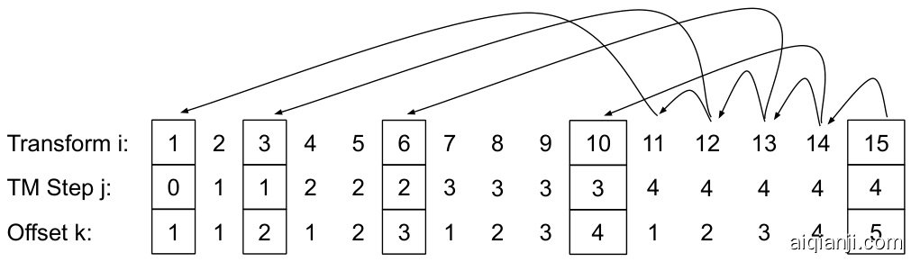
Figure 2: Mapping between transformer step and original Turing machine step.
图 2: Transformer步骤与原图灵机步骤的映射关系。
Embeddings and positional encodings Our construction needs a different positional encoding $\mathrm{pos}_{\mathrm{Dec}}:\mathbb{N}\to\mathbb{Q}^{d}$ for decoder:
嵌入和位置编码 我们的构造需要为解码器使用不同的位置编码 $\mathrm{pos}_{\mathrm{Dec}}:\mathbb{N}\to\mathbb{Q}^{d}$ :
$$
\mathrm{pos}_{\mathrm{Dec}}(i) = \left[
\begin{array}{@{}l@{}}
0,\ldots,0, \
0,\ldots,0, \
0,\ldots,0, \
1, g(i)+1, \frac{1}{g(i)+1}, \frac{1}{(g(i)+1)^2}, h(i), 0, 0, 0, 0
\end{array}
\right]
$$
$$
\mathrm{pos}_{\mathrm{Dec}}(i) = \left[
\begin{array}{@{}l@{}}
0,\ldots,0, \
0,\ldots,0, \
0,\ldots,0, \
1, g(i)+1, \frac{1}{g(i)+1}, \frac{1}{(g(i)+1)^2}, h(i), 0, 0, 0, 0
\end{array}
\right]
$$
where g(i) = j −1+√21+8i k and $h(i)=g(i+1)-g(i)$ . Note that $h(i)$ reduces to a binary indicator variable 1 n −1+√21+8i 
其中 g(i) = j −1+√21+8i k 且 $h(i)=g(i+1)-g(i)$ 。注意 $h(i)$ 可简化为二元指示变量 1 n −1+√21+8i $\mathbf{1}\left{
Induction Setup
归纳设置
We next show how to construct the decoder layers to produce the sequence of outputs $y_{1},y_{2},\dotsc$ , where ${\bf{{y}}}_{i}$ is given by:
我们接下来展示如何构建解码器层以生成输出序列 $y_{1},y_{2},\dotsc$ ,其中 ${\bf{{y}}}_{i}$ 由下式给出:
$$
\begin{array}{l l l}{\pmb{y}_ {i}}&{=}&{[\quad\mathbb{I}q^{g(i)}\mathbb{I},[\int s^{g(i)}\mathbb{I},c^{g(i)},}\ &&{0,\dots,0,}\ &&{\mathbf{0}_ {s},0,[\pi^{(i)}\mathbb{I},}\ &&{0,0,0,0,u_{1}^{(i)},u_{2}^{(i)},u_{3}^{(i)},u_{4}^{(i)}\quad]}\end{array}
$$
$$
\begin{array}{l l l}{\pmb{y}_ {i}}&{=}&{[\quad\mathbb{I}q^{g(i)}\mathbb{I},[\int s^{g(i)}\mathbb{I},c^{g(i)},}\ &&{0,\dots,0,}\ &&{\mathbf{0}_ {s},0,[\pi^{(i)}\mathbb{I},}\ &&{0,0,0,0,u_{1}^{(i)},u_{2}^{(i)},u_{3}^{(i)},u_{4}^{(i)}\quad]}\end{array}
$$
That is, at step $i$ of our sparse decoder ${\bf{{y}}}_ {i}$ , it will contain the information about the state of the turing machine $M$ at time $g(i)$ , the symbol under the head of $M$ at time $g(i)$ , and the current location of head of $M$ at time $g(i)$ . We also have a placeholder symbol $w$ and placeholder scalars $u_{1},u_{2},u_{3}$ , whose role will be clear from our construction.
也就是说,在我们稀疏解码器 ${\bf{{y}}}_ {i}$ 的第 $i$ 步时,它将包含图灵机 $M$ 在时间 $g(i)$ 的状态信息、$M$ 在时间 $g(i)$ 时磁头下的符号,以及 $M$ 在时间 $g(i)$ 时磁头的当前位置。我们还设置了一个占位符符号 $w$ 和占位标量 $u_{1},u_{2},u_{3}$,它们的作用将在后续构建过程中明确。
We consider as the starting vector for the decoder the vector
我们将解码器的起始向量视为向量
$$
\begin{array}{c c c c}{\pmb{y}_ {1}}&{=}&{[}&{[\begin{array}{l}{q_{\mathrm{init}}],[[\nrightarrow]],0,}\ &&{0,···,0,}\end{array}}\ &{\begin{array}{l}{\begin{array}{r l}&{0,···,0,}\ &{0,···,0}\end{array}}\ &{\begin{array}{r l}&{0,···,0}\end{array}}\end{array}]}\end{array}
$$
$$
\begin{array}{c c c c}{\pmb{y}_ {1}}&{=}&{[}&{[\begin{array}{l}{q_{\mathrm{init}}],[[\nrightarrow]],0,}\ &&{0,···,0,}\end{array}}\ &{\begin{array}{l}{\begin{array}{r l}&{0,···,0,}\ &{0,···,0}\end{array}}\ &{\begin{array}{r l}&{0,···,0}\end{array}}\end{array}]}\end{array}
$$
We assume that the start head is at $c^{(0)}=0$ , the initial state is $q^{(0)}=q_{\mathrm{init}}$ , and 
as we initialize from clean tape. We show the correctness of our construction by an inductive argument: we describe the architecture piece by piece and at the same time will show for every $r\geq0$ , our architecture constructs ${\pmb y}_ {r+1}$ from the previous vectors $(\pmb{y}{0},\dots,\pmb{y}{r})$ .
我们假设起始头位于 $c^{(0)}=0$,初始状态为 $q^{(0)}=q_{\mathrm{init}}$,且
(因为从空白带初始化)。我们通过归纳论证来展示构造的正确性:逐步描述架构的同时,将证明对于每个 $r\geq0$,我们的架构都能根据先前的向量 $(\pmb{y}_ {0},\dots,\pmb{y}_ {r})$ 构造出 ${\pmb y}_ {r+1}$。
Thus, assume that $y_{1},\ldots,y_{r}$ satisfy the properties stated above. Since we are using positional encodings, the actual input for the first layer of the decoder is the sequence
因此,假设 $y_{1},\ldots,y_{r}$ 满足上述性质。由于我们使用了位置编码 (positional encodings),解码器第一层的实际输入序列为
$$
y_{1}+\mathrm{pos}_ {\mathrm{Dec}}(1),y_{2}+\mathrm{pos}_ {\mathrm{Dec}}(2),\dots,y_{r}+\mathrm{pos}_{\mathrm{Dec}}(r).
$$
$$
y_{1}+\mathrm{pos}_ {\mathrm{Dec}}(1),y_{2}+\mathrm{pos}_ {\mathrm{Dec}}(2),\dots,y_{r}+\mathrm{pos}_{\mathrm{Dec}}(r).
$$
We denote by $\overline{{\mathbf{{y}}}}_ {i}$ the vector ${\bf{{y}}}_{i}$ plus its positional encoding. Thus we have $\forall1\leq i\leq r$ tha
我们记 $\overline{{\mathbf{{y}}}}_ {i}$ 为向量 ${\bf{{y}}}_{i}$ 加上其位置编码。因此对于 $\forall1\leq i\leq r$ 有
$$
\overline{\boldsymbol{y}}_i = \left[\begin{aligned}& \big[q^{g(i)}\big], \big[s^{g(i)}\big], c^{g(i)}, \& 0,\dots,0, \mathbf{0}_s, 0,\big[w^{(i)}\big], \& 1, g(i)+1, \frac{1}{g(i)+1}, \frac{1}{(g(i)+1)^2}, h(i), u_1^{(i)}, u_2^{(i)}, u_3^{(i)}, u_4^{(i)}\end{aligned}\right].
$$
$$
\overline{\boldsymbol{y}}_i = \left[\begin{aligned}& \big[q^{g(i)}\big], \big[s^{g(i)}\big], c^{g(i)}, \& 0,\dots,0, \mathbf{0}_s, 0,\big[w^{(i)}\big], \& 1, g(i)+1, \frac{1}{g(i)+1}, \frac{1}{(g(i)+1)^2}, h(i), u_1^{(i)}, u_2^{(i)}, u_3^{(i)}, u_4^{(i)}\end{aligned}\right].
$$
B.2.1 Layer 1: Simulate Transition Function
B.2.1 第一层:模拟转移函数
In this layer, we use the cross-attention between encoder and decoder to access the input string and a feed-forward network to simulate the transition function of $M$ . The first self attention in Eq. (5) is not used in this layer and we just produce the identity. This identity function is achieved by setting all queries, keys, values to be 0 everywhere plus the residual connection. Thus, we have $\pmb{p}_ {i}^{1}=\overline{{\pmb{y}}}_{i}$ .
在这一层中,我们利用编码器与解码器之间的交叉注意力机制来访问输入字符串,并通过前馈网络模拟 $M$ 的转移函数。方程(5)中的第一个自注意力机制在本层未被使用,我们仅生成恒等输出。该恒等函数通过将所有查询(query)、键(key)和值(value)设为0并结合残差连接实现,因此有 $\pmb{p}_ {i}^{1}=\overline{{\pmb{y}}}_{i}$。
Since ${\pmb p}_ {i}^{1}$ is of the form $[_,\cdot\cdot\cdot,_,1,g(i)+1,_,\ldots,]$ , we know by Lemma B.1 of Pérez et al. [72] that if we use ${\pmb p}_{i}^{1}$ to attend over the encoder we obtain
由于 ${\pmb p}_ {i}^{1}$ 的形式为 $[_,\cdot\cdot\cdot,_,1,g(i)+1,_,\ldots,]$ ,根据 Pérez 等人 [72] 的引理 B.1,我们知道若使用 ${\pmb p}_{i}^{1}$ 对编码器进行注意力计算,将得到
$$
\begin{array}{l c l}{{\mathrm{CROSSATTN}(p_{i}^{1},K^{\mathbf{e}},V^{\mathbf{e}})}}&{{=}}&{{[\quad0,\ldots,0,}}\ {{}}&{{}}&{{0,\ldots,0,}}\ {{}}&{{}}&{{[\alpha^{g(i)+1}],\beta^{g(i)+1},\mathbf{0}_{s},}}\ {{}}&{{}}&{{0,\ldots,0}}\end{array}
$$
$$
\begin{array}{l c l}{{\mathrm{CROSSATTN}(p_{i}^{1},K^{\mathbf{e}},V^{\mathbf{e}})}}&{{=}}&{{[\quad0,\ldots,0,}}\ {{}}&{{}}&{{0,\ldots,0,}}\ {{}}&{{}}&{{[\alpha^{g(i)+1}],\beta^{g(i)+1},\mathbf{0}_{s},}}\ {{}}&{{}}&{{0,\ldots,0}}\end{array}
$$
where $\alpha$ and $\beta$ are as defined in Eq. (21) of [72]. Thus in Eq. (4) we finally produce the vector ${\pmb a}_{i}^{1}$ given by
其中 $\alpha$ 和 $\beta$ 的定义见文献[72]的公式(21)。因此在公式(4)中,我们最终生成由 ${\pmb a}_{i}^{1}$ 给出的向量
$$
\begin{aligned}a_i^1 &= \mathrm{CrossAttn}(p_i^1, K^e, V^e) + p_i^1 \
&= \Big[\big[q^{g(i)}\big], \big[\boldsymbol{s}^{g(i)}\big], c^{g(i)}, 0,\dots,0, \&\quad \big[\boldsymbol{\alpha}^{g(i)+1}\big], \beta^{g(i)+1}, \big[\boldsymbol{w}^{(i)}\big], \&\quad \boldsymbol{1}, g(i)+1, \frac{1}{g(i)+1}, \frac{1}{(g(i)+1)^2}, h(i), u_1^{(i)}, u_2^{(i)}, u_3^{(i)}, u_4^{(i)}\Big]\end{aligned}
$$
$$
\begin{aligned}a_i^1 &= \mathrm{CrossAttn}(p_i^1, K^e, V^e) + p_i^1 \&= \Big[\big[q^{g(i)}\big], \big[\boldsymbol{s}^{g(i)}\big], c^{g(i)}, 0,\dots,0, \&\quad \big[\boldsymbol{\alpha}^{g(i)+1}\big], \beta^{g(i)+1}, \big[\boldsymbol{w}^{(i)}\big], \&\quad \boldsymbol{1}, g(i)+1, \frac{1}{g(i)+1}, \frac{1}{(g(i)+1)^2}, h(i), u_1^{(i)}, u_2^{(i)}, u_3^{(i)}, u_4^{(i)}\Big]\end{aligned}
$$
As the final piece of the first decoder layer we use a function $O_{1}(\cdot)$ (Eq. (3)) that satisfies the following lemma.
在第一解码层的最后部分,我们使用满足以下引理的函数 $O_{1}(\cdot)$ (式(3))。
Lemma 6 (Lemma B.2 [72]). There exists a two-layer feed-forward network $O_{1}:\mathbb{Q}^{d}\to\mathbb{Q}^{d}$ such that with input vector ${\pmb a}_{i}^{1}$ (Eq. (7)) produces as output
引理6 (引理B.2 [72])。存在一个双层前馈网络 $O_{1}:\mathbb{Q}^{d}\to\mathbb{Q}^{d}$,当输入向量 ${\pmb a}_{i}^{1}$ (式(7))时,其输出为
$$
\begin{array}{c c l}{{{\cal O}_ {1}({\pmb a}_{i}^{1})}}&{{=}}&{{[\quad0,\ldots,0,}}\ {{}}&{{}}&{{\underline{{{{\big[\quad q^{g(i)+1}\big]}}}},\stackrel{[]}{\left[\begin{array}{c}{{v^{g(i)}}}\end{array}\right]},m^{g(i)},0,0,0,0}}\ {{}}&{{}}&{{0,\ldots,0,}}\ {{}}&{{}}&{{0,\ldots,0}}\end{array}\quad\begin{array}{r l}{{}}&{{}}\ {{{\big]}}}&{{}}&{{}}\end{array}
$$
$$
\begin{array}{c c l}{{{\cal O}_ {1}({\pmb a}_{i}^{1})}}&{{=}}&{{[\quad0,\ldots,0,}}\ {{}}&{{}}&{{\underline{{{{\big[\quad q^{g(i)+1}\big]}}}},\stackrel{[]}{\left[\begin{array}{c}{{v^{g(i)}}}\end{array}\right]},m^{g(i)},0,0,0,0}}\ {{}}&{{}}&{{0,\ldots,0,}}\ {{}}&{{}}&{{0,\ldots,0}}\end{array}\quad\begin{array}{r l}{{}}&{{}}\ {{{\big]}}}&{{}}&{{}}\end{array}
$$
That is, function $O_{1}(\cdot)$ simulates transition $\delta\bigl(q^{g(i)},s^{g(i)}\bigr)$ to construct $\mathbb{[}q^{g(i)+1}\mathbb{]},\mathbb{[}v^{g(i)}\mathbb{]}$ , and $m^{g(i)}$ besides some other linear transformations.
即,函数 $O_{1}(\cdot)$ 通过模拟转移 $\delta\bigl(q^{g(i)},s^{g(i)}\bigr)$ 来构造 $\mathbb{[}q^{g(i)+1}\mathbb{]},\mathbb{[}v^{g(i)}\mathbb{]}$ 以及 $m^{g(i)}$,同时执行其他线性变换。
Thus, finally the output of the first decoder layer is
因此,最终第一层解码器的输出是
$$
\begin{array}{r l}{z_{i}^{1}=O_{1}(a_{i}^{1})+a_{i}^{1}}&{=\phantom{-}[\phantom{-}[\phantom{-}[\phantom{-}q^{g(i)}]],[\phantom{-}s^{g(i)}]],c^{g(i)},}\ &{\phantom{-}[\phantom{-}[\phantom{-}[\phantom{-}]][q^{g(i)}]],[\phantom{-}v^{g(i)}]],m^{g(i)},0,0,0,0,}\ &{\phantom{-}[\phantom{-}[\phantom{-}]],}\ &{\phantom{-}1,g(i)+1,\frac{1}{g(i)+1},\frac{1}{(g(i)+1)^{2}},h(i),u_{1}^{(i)},u_{2}^{(i)},u_{3}^{(i)},u_{4}^{(i)}]\phantom{-[\phantom{-}[\phantom{-}]]}}\end{array}
$$
$$
\begin{array}{r l}{z_{i}^{1}=O_{1}(a_{i}^{1})+a_{i}^{1}}&{=\phantom{-}[\phantom{-}[\phantom{-}[\phantom{-}q^{g(i)}]],[\phantom{-}s^{g(i)}]],c^{g(i)},}\ &{\phantom{-}[\phantom{-}[\phantom{-}[\phantom{-}]][q^{g(i)}]],[\phantom{-}v^{g(i)}]],m^{g(i)},0,0,0,0,}\ &{\phantom{-}[\phantom{-}[\phantom{-}]],}\ &{\phantom{-}1,g(i)+1,\frac{1}{g(i)+1},\frac{1}{(g(i)+1)^{2}},h(i),u_{1}^{(i)},u_{2}^{(i)},u_{3}^{(i)},u_{4}^{(i)}]\phantom{-[\phantom{-}[\phantom{-}]]}}\end{array}
$$
B.2.2 Layer 2: Finding Head Node
B.2.2 第二层:寻找头节点
In this layer, we only use the feed-forward network to evaluate the next location of the head. The self-attention and cross-attention are set to be the identity function, so $\pmb{a}_ {i}^{2}=\pmb{p}_{i}^{2}=\pmb{z}_{i}^{1}$ . Recall that $c^{g(i)}$ is the cell to which $M$ is pointing to at time $g(i)$ , and that it satisfies the following recursion $c^{g(i)+1}=c^{g(i)}+m^{g(i)}$ , which can be expanded to see that that $c^{g(i)+1}=m^{(0)}+m^{(1)}+\bar{\cdot}\cdot\cdot+m^{g(i)}$ . Its not difficult to see that a two layer network with non-linearity can compute $c^{g(i)+1}/(g(i)+1)$ and $c^{g(i)}/(g(i)+1)$ from $c^{g(i)}$ , $m^{g(i)}$ , and $1/(g(i)+1)$ using the relation $c^{g(i)+1}=c^{g(i)}+m^{g(i)}$ . At the end of layer 2, we obtain
在这一层中,我们仅使用前馈网络来评估头部的下一个位置。自注意力(self-attention)和交叉注意力(cross-attention)被设置为恒等函数,因此$\pmb{a}_ {i}^{2}=\pmb{p}_ {i}^{2}=\pmb{z}_{i}^{1}$。回顾$c^{g(i)}$是$M$在时刻$g(i)$指向的单元格,它满足以下递归关系$c^{g(i)+1}=c^{g(i)}+m^{g(i)}$,可以展开得到$c^{g(i)+1}=m^{(0)}+m^{(1)}+\bar{\cdot}\cdot\cdot+m^{g(i)}$。不难看出,带有非线性的两层网络可以通过关系式$c^{g(i)+1}=c^{g(i)}+m^{g(i)}$,从$c^{g(i)}$、$m^{g(i)}$和$1/(g(i)+1)$计算出$c^{g(i)+1}/(g(i)+1)$和$c^{g(i)}/(g(i)+1)$。在第2层结束时,我们得到
$$
\begin{array}{l c l}{{z_{i}^{2}={\cal O}_ {2}(a_{i}^{2})+a_{i}^{2}}}&{{=}}&{{[\phantom{-}[\phantom{-}[\phantom{-}q^{g(i)}]],[s^{g(i)}],c^{g(i)},}}\ {{}}&{{}}&{{[\phantom{-}q^{g(i)+1}],[v^{g(i)}],c^{g(i)+1},\frac{1}{g(i)+1},\frac{c^{g(i)+1}}{(g(i)+1)^{2}},\frac{c^{g(i)+1}}{g(i)+1},\frac{c^{g(i)}}{g(i)+1},}}\ {{}}&{{}}&{{[\phantom{-}\alpha^{g(i)+1}],\beta^{g(i)+1},[w^{(i)}],}}\ {{}}&{{}}&{{1,g(i)+1,\frac{1}{g(i)+1},\frac{1}{(g(i)+1)^{2}},h(i),u_{1}^{(i)},u_{2}^{(i)},u_{3}^{(i)},u_{4}^{(i)}}}\end{array}
$$
$$
\begin{array}{l c l}{{z_{i}^{2}={\cal O}_ {2}(a_{i}^{2})+a_{i}^{2}}}&{{=}}&{{[\phantom{-}[\phantom{-}[\phantom{-}q^{g(i)}]],[s^{g(i)}],c^{g(i)},}}\ {{}}&{{}}&{{[\phantom{-}q^{g(i)+1}],[v^{g(i)}],c^{g(i)+1},\frac{1}{g(i)+1},\frac{c^{g(i)+1}}{(g(i)+1)^{2}},\frac{c^{g(i)+1}}{g(i)+1},\frac{c^{g(i)}}{g(i)+1},}}\ {{}}&{{}}&{{[\phantom{-}\alpha^{g(i)+1}],\beta^{g(i)+1},[w^{(i)}],}}\ {{}}&{{}}&{{1,g(i)+1,\frac{1}{g(i)+1},\frac{1}{(g(i)+1)^{2}},h(i),u_{1}^{(i)},u_{2}^{(i)},u_{3}^{(i)},u_{4}^{(i)}}}\end{array}
$$
B.2.3 Layer 3: Distinguishing Node Type
B.2.3 第三层:区分节点类型
This is an additional layer (not present in the work of [72]), where we propagate computations in our sparse graph. In particular, we will use this layer to “compute” or accumulate state in intermediate nodes. We make this clear below. The self-attention and cross-attention are all set to be the identity function, so ${\bf{}}a_{i}^{3}={\bf{}}p_{i}^{3}=z_{i}^{2}$ . In this layer, we only use the dense attention layers to select the newly computed states or to continue with previous states. Using idea similar to Lemma B.6 of [72], we can construct a dense network such that
这是一个额外的层(在[72]的工作中未出现),我们在稀疏图中传播计算。具体来说,我们将使用这一层来“计算”或累积中间节点的状态。下文将对此进行详细说明。自注意力(self-attention)和交叉注意力(cross-attention)均设置为恒等函数,因此 ${\bf{}}a_{i}^{3}={\bf{}}p_{i}^{3}=z_{i}^{2}$。在这一层中,我们仅使用密集注意力层来选择新计算的状态或延续之前的状态。采用类似于[72]中引理B.6的思路,我们可以构建一个密集网络,使得
$$
O([x,y,z,b]) =\begin{cases}[{\bf 0}, {\bf 0}, {\bf 0}, 0] & \text{if } b = 1, \
[{\bf 0}, z-y, -z, 0] & \text{if } b = 0.\end{cases}
$$
$$
O([x,y,z,b]) =\begin{cases}[{\bf 0}, {\bf 0}, {\bf 0}, 0] & \text{if } b = 1, \
[{\bf 0}, z-y, -z, 0] & \text{if } b = 0.\end{cases}
$$
The negatives are generated to offset results from skip connection. We utilize such network to switch Turing machine state and position embedding for intermediate steps to the values received from
负面结果用于抵消跳跃连接的结果。我们利用此类网络将图灵机状态和中间步骤的位置嵌入切换为从接收到的值
previous time step and do nothing for compute nodes. We use $h(i)$ as the flipping bit $b$ . Thus, at end of layer 3, we obtain
前一时间步并对计算节点不做任何处理。我们使用 $h(i)$ 作为翻转位 $b$。因此,在第三层结束时,我们得到
$$
\begin{array}{r c l}{{z_{i}^{3}={\cal O}_ {3}(a_{i}^{3})+a_{i}^{3}}}&{{=}}&{{\big[\quad0,\ldots,0,}}\ {{}}&{{}}&{{\big[\hat{q}^{(i)}\big],\big[\hat{v}^{(i)}\big],\hat{c}^{(i)},\frac{1}{g(i)+1},\frac{1}{(g(i)+1)^{2}},\frac{c^{g(i)+1}}{g(i)+1},\hat{u}_ {4}^{(i)},}}\ {{}}&{{}}&{{\big[\hat{\alpha}^{(i)}\big],\hat{\beta}^{(i)},{\bf0}_{s},}}\ {{}}&{{}}&{{1,\hat{u}_ {1}^{(i)},\hat{u}_ {2}^{(i)},\hat{u}_{3}^{(i)},h(i),0,0,0,0}}\end{array}
$$
$$
\begin{array}{r c l}{{z_{i}^{3}={\cal O}_ {3}(a_{i}^{3})+a_{i}^{3}}}&{{=}}&{{\big[\quad0,\ldots,0,}}\ {{}}&{{}}&{{\big[\hat{q}^{(i)}\big],\big[\hat{v}^{(i)}\big],\hat{c}^{(i)},\frac{1}{g(i)+1},\frac{1}{(g(i)+1)^{2}},\frac{c^{g(i)+1}}{g(i)+1},\hat{u}_ {4}^{(i)},}}\ {{}}&{{}}&{{\big[\hat{\alpha}^{(i)}\big],\hat{\beta}^{(i)},{\bf0}_ {s},}}\ {{}}&{{}}&{{1,\hat{u}_ {1}^{(i)},\hat{u}_ {2}^{(i)},\hat{u}_{3}^{(i)},h(i),0,0,0,0}}\end{array}
$$
where we used $h(i)$ for selecting old states. In particular,
我们使用 $h(i)$ 来选择旧状态。具体来说,
• We copy the input state and head position as is for intermediate nodes. We do not need to transition to next Turing machine states in these nodes.
• 对于中间节点,我们直接复制输入状态和磁头位置。这些节点无需切换到图灵机的下一状态。
$$
\begin{aligned}\hat{q}^{(i)} &= \begin{cases}q^{g(i)+1} & \text{if } h(i) = 1 \
q^{g(i)} & \text{if } h(i) = 0\end{cases}, \\hat{v}^{(i)} &= \begin{cases}v^{g(i)} & \text{if } h(i) = 1 \
w^{(i)} & \text{if } h(i) = 0\end{cases}, \\hat{c}^{(i)} &= \begin{cases}c^{g(i)+1} &\text{if } h(i) = 1 \
c^{g(i)} & \text{if } h(i) = 0\end{cases}.\end{aligned}
$$
$$
\begin{aligned}\hat{q}^{(i)} &= \begin{cases}q^{g(i)+1} & \text{if } h(i) = 1 \
q^{g(i)} & \text{if } h(i) = 0\end{cases}, \\hat{v}^{(i)} &= \begin{cases}v^{g(i)} & \text{if } h(i) = 1 \
w^{(i)} & \text{if } h(i) = 0\end{cases}, \\hat{c}^{(i)} &= \begin{cases}c^{g(i)+1} &\text{if } h(i) = 1 \
c^{g(i)} & \text{if } h(i) = 0\end{cases}.\end{aligned}
$$
• To preserve the symbol under the head for intermediate nodes, we copy the previous symbol to $\alpha$ location and set $\beta=g(i)+1$ , as the symbol at $\alpha$ location will be copied as the symbol under head for next transformer step by the final transformation layer if $\bar{\beta=g(i)+1}$ . Thus, we correctly preserve the previous symbol under head as Turing machine does not transition these nodes. For compute nodes, things happen as usual.
• 为保留中间节点头部下方的符号,我们将前一个符号复制到 $\alpha$ 位置,并将 $\beta$ 设为 $g(i)+1$。因为当 $\bar{\beta=g(i)+1}$ 时,$\alpha$ 位置的符号会通过最终转换层逐步作为头部下方符号传递到下一个Transformer步骤。这样我们就能像图灵机不转移这些节点时那样,正确保留头部下方的先前符号。对于计算节点,则按常规流程处理。
$$
\begin{aligned}\hat{\alpha}^{(i)} &= \begin{cases}\alpha^{g(i)+1} & \text{if } h(i) = 1 \
s^{g(i)} & \text{if } h(i) = 0\end{cases}, \ \hat{\beta}^{(i)} &= \begin{cases}\beta^{g(i)+1} & \text{if } h(i) = 1 \
g(i)+1 & \text{if } h(i) = 0\end{cases}.\end{aligned}
$$
$$
\begin{aligned}\hat{\alpha}^{(i)} &= \begin{cases}\alpha^{g(i)+1} & \text{if } h(i) = 1 \
s^{g(i)} & \text{if } h(i) = 0\end{cases}, \ \hat{\beta}^{(i)} &= \begin{cases}\beta^{g(i)+1} & \text{if } h(i) = 1 \
g(i)+1 & \text{if } h(i) = 0\end{cases}.\end{aligned}
$$
• Finally for the intermediate nodes, we copy the position embedding corresponding to current best symbol $w$ , which is stored in $u_{1},u_{2},u_{3}$ . For compute node, we let the position embedding correspond to current Turing machine step.
• 最后对于中间节点,我们复制与当前最佳符号 $w$ 对应的位置嵌入,该符号存储在 $u_{1},u_{2},u_{3}$ 中。对于计算节点,我们让位置嵌入对应于当前图灵机步骤。
$$
\begin{aligned}
\hat{u}_1^{(i)} &= \begin{cases}
g(i)+1 & \text{if } h(i)=1 \
u_1^{(i)} & \text{if } h(i)=0
\end{cases}, \quad
\hat{u}_2^{(i)} = \begin{cases}
\frac{1}{g(i)+1} & \text{if } h(i)=1 \
u_2^{(i)} & \text{if } h(i)=0
\end{cases}, \
\hat{u}_3^{(i)} &= \begin{cases}
\frac{1}{(g(i)+1)^2} & \text{if } h(i)=1 \
u_3^{(i)} & \text{if } h(i)=0
\end{cases}, \quad
\hat{u}_4^{(i)} = \begin{cases}
\frac{c^{g(i)}}{g(i)+1} & \text{if } h(i)=1 \
u_4^{(i)} & \text{if } h(i)=0
\end{cases}.
\end{aligned}
$$
$$
\begin{aligned}
\hat{u}_1^{(i)} &= \begin{cases}
g(i)+1 & \text{if } h(i)=1 \
u_1^{(i)} & \text{if } h(i)=0
\end{cases}, \quad
\hat{u}_2^{(i)} = \begin{cases}
\frac{1}{g(i)+1} & \text{if } h(i)=1 \
u_2^{(i)} & \text{if } h(i)=0
\end{cases}, \
\hat{u}_3^{(i)} &= \begin{cases}
\frac{1}{(g(i)+1)^2} & \text{if } h(i)=1 \
u_3^{(i)} & \text{if } h(i)=0
\end{cases}, \quad
\hat{u}_4^{(i)} = \begin{cases}
\frac{c^{g(i)}}{g(i)+1} & \text{if } h(i)=1 \
u_4^{(i)} & \text{if } h(i)=0
\end{cases}.
\end{aligned}
$$
For further simplification note that $g(i+1)=g(i)$ if $h(i)=0$ else $g(i)+1$ when $h(i)=1$ . With this fact, we can conclude that $\hat{q}^{(i)}=q^{g(i+1)}$ and $\hat{c}^{(i)}=c^{g(i+1)}$ . Thus, we can write,
为简化表述,注意到当 $h(i)=0$ 时 $g(i+1)=g(i)$ ,否则当 $h(i)=1$ 时 $g(i+1)=g(i)+1$ 。由此可得 $\hat{q}^{(i)}=q^{g(i+1)}$ 且 $\hat{c}^{(i)}=c^{g(i+1)}$ ,因此可表示为
$$
\begin{array}{r l r l}{z_{i}^{3}}&{=}&{[}&{0,\ldots,0,}\ &{}&&{\mathbb{I}_ {q}^{g(i+1)}\mathbb{I},\mathbb{I}\hat{v}^{(i)}\mathbb{I},c^{g(i+1)},\frac{1}{g(i)+1},\frac{1}{(g(i)+1)^{2}},\frac{c^{g(i)+1}}{g(i)+1},\hat{u}_ {4}^{(i)},}\ &{}&&{\mathbb{I}\hat{\alpha}^{(i)}\mathbb{I},\hat{\beta}^{(i)},\mathbf{0}{s},}\ &{}&&{1,\hat{u}{1}^{(i)},\hat{u}_ {2}^{(i)},\hat{u}_{3}^{(i)},h(i),0,0,0,0}\end{array}
$$
$$
\begin{array}{r l r l}{z_{i}^{3}}&{=}&{[}&{0,\ldots,0,}\ &{}&&{\mathbb{I}_ {q}^{g(i+1)}\mathbb{I},\mathbb{I}\hat{v}^{(i)}\mathbb{I},c^{g(i+1)},\frac{1}{g(i)+1},\frac{1}{(g(i)+1)^{2}},\frac{c^{g(i)+1}}{g(i)+1},\hat{u}_ {4}^{(i)},}\ &{}&&{\mathbb{I}\hat{\alpha}^{(i)}\mathbb{I},\hat{\beta}^{(i)},\mathbf{0}_ {s},}\ &{}&&{1,\hat{u}_ {1}^{(i)},\hat{u}_ {2}^{(i)},\hat{u}_{3}^{(i)},h(i),0,0,0,0}\end{array}
$$
B.2.4 Layer 4: Finding next symbol on tape
B.2.4 第四层:在纸带上寻找下一个符号
To find the symbol on tape under next head position $c^{g(i)+1}$ , we try to find what was written last at the location $c^{g(i)+1}$ . To facilitate this, following [72], we define $\ell(j)$ to be the last time (previous to $j$ ) in which $M$ was pointing to position $c^{(j)}$ , or it is $j-1$ if this is the first time that $M$ is pointing to $c^{(j)}$ . Recall $j$ is the Turing machine step counter, which is different from sparse transformer step $i$ . [72] could utilize full attention mechanism to find $v^{\ell(j+1)}$ at one go, but we have to do it over multiple steps owing to our sparse attention mechanism.
为了找到磁带上下一个磁头位置 $c^{g(i)+1}$ 处的符号,我们尝试找出在位置 $c^{g(i)+1}$ 最后一次写入的内容。为此,参考 [72],我们定义 $\ell(j)$ 为 $M$ 指向位置 $c^{(j)}$ 的最后一次时间(在 $j$ 之前),如果这是 $M$ 首次指向 $c^{(j)}$,则取值为 $j-1$。注意,$j$ 是图灵机步骤计数器,不同于稀疏 Transformer 步骤 $i$。[72] 可以利用完整的注意力机制一次性找到 $v^{\ell(j+1)}$,但由于我们的稀疏注意力机制,必须分多步完成。
We use similar query, key, value functions as used for full attention by $[72]\forall i$ :
我们采用与[72]中全注意力机制相似的查询(query)、键(key)、值(value)函数 $\forall i$:
$$
\begin{array}{l l l}{{Q_{4}(z_{i}^{3})}}&{{=}}&{{[\quad0,\ldots,0}}\ {{}}&{{}}&{{0,\ldots,0,}}\ {{}}&{{}}&{{0,\ldots,0,}}\ {{}}&{{}}&{{0,{\frac{c^{g(i)+1}}{g(i)+1}},{\frac{1}{g(i)+1}},{\frac{1}{3(g(i)+1)^{2}}},0,0,0,0,0,0.}}\end{array}
$$
$$
\begin{array}{l l l}{{Q_{4}(z_{i}^{3})}}&{{=}}&{{[\quad0,\ldots,0}}\ {{}}&{{}}&{{0,\ldots,0,}}\ {{}}&{{}}&{{0,\ldots,0,}}\ {{}}&{{}}&{{0,{\frac{c^{g(i)+1}}{g(i)+1}},{\frac{1}{g(i)+1}},{\frac{1}{3(g(i)+1)^{2}}},0,0,0,0,0,0.}}\end{array}
$$
$$
\begin{aligned}
K_4(z_i^3) &= \left[
\begin{array}{@{}l@{}}
0,\ldots,0, \
0,\ldots,0, \
0,\ldots,0, \
0, \hat{u}_2^{(i)}, \hat{u}_4^{(i)}, \hat{u}_3^{(i)}, 0, 0, 0, 0, 0, 0
\end{array}
\right], \
V_4(z_i^3) &= \left[
\begin{array}{@{}l@{}}
0,\ldots,0, \
0,\ldots,0, \
\mathbf{0}_s, 0, \left[\hat{\boldsymbol{\nu}}^{(i)}\right], \
0, 0, 0, 0, 0, \hat{u}_1^{(i)}, \hat{u}_2^{(i)}, \hat{u}_3^{(i)}, \hat{u}_4^{(i)}
\end{array}
\right].
\end{aligned}
$$
$$
\begin{aligned}
K_4(z_i^3) &= \left[
\begin{array}{@{}l@{}}
0,\ldots,0, \
0,\ldots,0, \
0,\ldots,0, \
0, \hat{u}_2^{(i)}, \hat{u}_4^{(i)}, \hat{u}_3^{(i)}, 0, 0, 0, 0, 0, 0
\end{array}
\right], \
V_4(z_i^3) &= \left[
\begin{array}{@{}l@{}}
0,\ldots,0, \
0,\ldots,0, \
\mathbf{0}_s, 0, \left[\hat{\boldsymbol{\nu}}^{(i)}\right], \
0, 0, 0, 0, 0, \hat{u}_1^{(i)}, \hat{u}_2^{(i)}, \hat{u}_3^{(i)}, \hat{u}_4^{(i)}
\end{array}
\right].
\end{aligned}
$$
It is clear that the three functions are linear transformations and thus they can be defined by feedforward networks. Notice that the query vector is always formed using current time step position embedding, whereas key and value vectors are formed using copied over entries for intermediate nodes and using current entries only for compute node.
显然,这三个函数都是线性变换,因此可以通过前馈网络来定义。需要注意的是,查询向量总是使用当前时间步的位置嵌入来构建,而键和值向量则针对中间节点使用复制过来的条目构建,仅针对计算节点使用当前条目。
Pérez et al. [72] find the desired $v^{l(j+1)}$ as $v^{m(j)}$ using full attention, where
Pérez et al. [72] 通过完全注意力机制找到所需的 $v^{l(j+1)}$ 作为 $v^{m(j)}$ ,其中
$$
m(t)=\operatorname*{argmin}_ {m\in{0,\ldots,t}}\chi_{t}^{j}=\operatorname*{argmin}_ {m\in{0,\ldots,t}}|\langle Q_{4}(z_{j}^{3}),K_{4}(z_{m}^{3})\rangle|
$$
$$
m(t)=\operatorname*{argmin}_ {m\in{0,\ldots,t}}\chi_{t}^{j}=\operatorname*{argmin}_ {m\in{0,\ldots,t}}|\langle Q_{4}(z_{j}^{3}),K_{4}(z_{m}^{3})\rangle|
$$
Note the minimization is only over Turing machine steps, i.e. over compute nodes in our case. We show below that we can estimates $m(j)$ by parts using sparse attention mechanism. The main idea is just to notice that minimization problem $\mathrm{min}_ {m\in{0,\ldots,t}}\chi_{t}^{j}$ can be expressed as $\operatorname*{min}{\cdot\cdot\cdot\operatorname*{min}{\operatorname*{min}{\chi_{0}^{j},\chi_{1}^{j}},\chi_{2}^{j}},...,\chi_{t}^{j}}$ by the associativity property.
注意最小化仅针对图灵机步骤,即在我们案例中的计算节点。下文我们将展示如何通过稀疏注意力机制分段估计 $m(j)$。核心思路是注意到最小化问题 $\mathrm{min}_ {m\in{0,\ldots,t}}\chi_{t}^{j}$ 可借助结合律性质表达为 $\operatorname*{min}{\cdot\cdot\cdot\operatorname*{min}{\operatorname*{min}{\chi_{0}^{j},\chi_{1}^{j}},\chi_{2}^{j}},...,\chi_{t}^{j}}$。
By definition of our graph $D$ , at every intermediate node $i$ of the form $j(j+1)/2+k$ , i.e. where $k>0$ , $g(i)=j$ and $h(i)=0$ , we will attend over node $k(k+1)/2$ and best till now copied from $i-1$ . The node $k(k+1)/2$ is never an intermediate node as $h(k(k+1)/2)=1$ for all $k$ and in fact corresponds to Turing machine’s step $k$ . This will help us select the key and value corresponding to min between node $k(k+1)/2$ and $i-1$ . In other words, at node $i$ of the form $j(j+1)^{\intercal}/2+k$ we would have evaluated $m(k)$ and corresponding value selected:
根据我们对图 $D$ 的定义,在每个形式为 $j(j+1)/2+k$ 的中间节点 $i$ (即 $k>0$ 时,$g(i)=j$ 且 $h(i)=0$ ),我们将关注节点 $k(k+1)/2$ 以及从 $i-1$ 复制的最佳结果。节点 $k(k+1)/2$ 永远不会是中间节点,因为对所有 $k$ 都有 $h(k(k+1)/2)=1$,实际上它对应图灵机的第 $k$ 步。这将帮助我们选择节点 $k(k+1)/2$ 和 $i-1$ 之间最小值对应的键和值。换句话说,在形式为 $j(j+1)^{\intercal}/2+k$ 的节点 $i$ 处,我们将评估 $m(k)$ 并选择相应的值:
$$
w^{\left(j\left(j+1\right)/2+k+1\right)}=\hat{v}^{m\left(k-1\right)}
$$
$$
w^{\left(j\left(j+1\right)/2+k+1\right)}=\hat{v}^{m\left(k-1\right)}
$$
and similarly for $u$ ’s. So after going through all the intermediate nodes, finally at the next compute node, i.e. when $k=j+1$ , we will obtain the minimum value over all of $0,1,...,j$ . This implies at a compute node will be able to recover $\ell(g(i)+1)$ and its corresponding value as shown in Lemma B.4 of [72]. Then we have that ${\pmb p}_{i}^{4}$ is given by
对于 $u$ 的情况同理。因此,在遍历所有中间节点后,最终在下一个计算节点(即当 $k=j+1$ 时),我们将获得 $0,1,...,j$ 上的最小值。这意味着计算节点能够恢复 $\ell(g(i)+1)$ 及其对应的值,如[72]中的引理B.4所示。于是可得 ${\pmb p}_{i}^{4}$ 的表达式为
$$
\begin{array}{r c l}{p_{i}^{4}}&{=}&{\mathrm{ATTN}_ {D}(Z_{i}^{3})+z_{i}^{3}}\ &{=}&{[\begin{array}{c c c}{0,\dots,0,}\ &&{[q^{g(i+1)}],[\widehat{v}^{(i)}],c^{g(i+1)},0,\frac{c^{g(i)+1}}{g(i)+1},\widehat{u}_ {4}^{(i)},}\end{array}}\ &&{\begin{array}{c c c}{\big[\widehat{\alpha}^{(i)}\big],\widehat{\beta}^{(i)},[[w^{(i+1)}]],}\ {1,\widehat{u}_ {1}^{(i)},\widehat{u}_ {2}^{(i)},\widehat{u}_ {3}^{(i)},h(i),u_{1}^{(i+1)},u_{2}^{(i+1)},u_{3}^{(i+1)},u_{4}^{(i+1)}}\end{array}}\end{array}
$$
$$
\begin{array}{r c l}{p_{i}^{4}}&{=}&{\mathrm{ATTN}_ {D}(Z_{i}^{3})+z_{i}^{3}}\ &{=}&{[\begin{array}{c c c}{0,\dots,0,}\ &&{[q^{g(i+1)}],[\widehat{v}^{(i)}],c^{g(i+1)},0,\frac{c^{g(i)+1}}{g(i)+1},\widehat{u}_ {4}^{(i)},}\end{array}}\ &&{\begin{array}{c c c}{\big[\widehat{\alpha}^{(i)}\big],\widehat{\beta}^{(i)},[[w^{(i+1)}]],}\ {1,\widehat{u}_ {1}^{(i)},\widehat{u}_ {2}^{(i)},\widehat{u}_ {3}^{(i)},h(i),u_{1}^{(i+1)},u_{2}^{(i+1)},u_{3}^{(i+1)},u_{4}^{(i+1)}}\end{array}}\end{array}
$$
The cross-attention and feed-forward network are set to be identity, so $z_{i}^{4}=a_{i}^{4}=p_{i}^{4}$ .
交叉注意力层和前馈网络被设置为恒等映射,因此 $z_{i}^{4}=a_{i}^{4}=p_{i}^{4}$。
B.2.5 Final transformation
B.2.5 最终转换
We finish our construction by using the final transformation function $F(\cdot)$ from the corresponding lemma from Pérez et al. [72], with a slight modification.
我们通过使用 Pérez 等人 [72] 对应引理中的最终转换函数 $F(\cdot)$ 来完成构建,并稍作修改。
Lemma 7 (Lemma B.5 [72]). There exists a function $F:\mathbb{Q}^{d}\to\mathbb{Q}^{d}$ defined by a feed-forward network such that
引理7 (引理 B.5 [72])。存在一个由前馈网络定义的函数 $F:\mathbb{Q}^{d}\to\mathbb{Q}^{d}$ 使得
$$
\begin{array}{l l l l}{{\cal F}(z_{r}^{4})}&{{=}}&{{[}}&{{[[q^{g(r+1)}]],[[s^{g(r+1))}]],c^{g(r+1)},}}\ {{}}&{{}}&{{}}&{{}}\ {{}}&{{}}&{{}}&{{{0,...,0,}}}\ {{}}&{{}}&{{{\bf0}_ {s},0,[[w^{(r+1)}]],}}\ {{}}&{{}}&{{}}&{{{0,0,0,0,0,u_{1}^{(r+1)},u_{2}^{(r+1)},u_{3}^{(r+1)},u_{4}^{(r+1)}]}}}\ {{}}&{{=}}&{{y_{r+1}}}\end{array}
$$
$$
\begin{array}{l l l l}{{\cal F}(z_{r}^{4})}&{{=}}&{{[}}&{{[[q^{g(r+1)}]],[[s^{g(r+1))}]],c^{g(r+1)},}}\ {{}}&{{}}&{{}}&{{}}\ {{}}&{{}}&{{}}&{{{0,...,0,}}}\ {{}}&{{}}&{{{\bf0}_ {s},0,[[w^{(r+1)}]],}}\ {{}}&{{}}&{{}}&{{{0,0,0,0,0,u_{1}^{(r+1)},u_{2}^{(r+1)},u_{3}^{(r+1)},u_{4}^{(r+1)}]}}}\ {{}}&{{=}}&{{y_{r+1}}}\end{array}
$$
The modification is to let $w,u_{1},u_{2},u_{3}$ to pass through. This yields the desired input to transformer at next time step for both intermediate and compute node, thereby concluding our induction.
修改是让 $w,u_{1},u_{2},u_{3}$ 通过。这为下一时间步的中间节点和计算节点提供了所需的Transformer输入,从而完成了我们的归纳。
C Limitations
C 限制
Finally, we show that sparse attention mechanisms can not universally replace dense attention mechanisms, i.e. there is no free lunch. We demonstrate a natural task which can be solved by the full attention mechanism in $O(1)$ -layers. However, under standard complexity theoretic assumptions, we show that this problem will require $\tilde{\Omega}(n)$ -layers for any sparse attention layers with ${\tilde{O}}(n)$ edges (not just BIGBIRD). (We use the standard notation $\tilde{\Omega}(n)$ to hide the dependence on poly-logarithmic factors. )
最后,我们证明稀疏注意力机制无法普遍替代密集注意力机制,即不存在免费午餐。我们展示了一个可由完整注意力机制在 $O(1)$ 层内解决的自然任务。然而,在标准计算复杂性理论假设下,我们证明该问题对于任何具有 ${\tilde{O}}(n)$ 条边的稀疏注意力层 (不仅限于BIGBIRD) 都需要 $\tilde{\Omega}(n)$ 层才能解决。(此处使用标准符号 $\tilde{\Omega}(n)$ 来隐藏对多对数因子的依赖。)
We consider the simple problem of finding the furthest vector for each vector in the given sequence of length $n$ and dimension $d\in\Omega(\log^{2}n)$ . The assumption on the dimension is mild , as in many situations the dimension $d=768$ is actually comparable to the number of $n$ .
我们考虑一个简单问题:在给定长度为 $n$、维度为 $d\in\Omega(\log^{2}n)$ 的向量序列中,为每个向量寻找最远向量。该维度假设是温和的,因为在许多情况下,维度 $d=768$ 实际上与 $n$ 的数量级相当。
Task 1. Given $n$ unit vectors ${u_{1},\ldots,u_{n}}$ , each in $\mathbb{R}^{d}$ where $d~=~\Theta(\log^{2}n)$ , compute $f(u_{1},\dots,u_{n})\to(u_{1^{ * }},\dots,u_ {n^{ * }})$ where for a fixed $j\in[n]$ , we define $j^{ * }=\arg\operatorname*{max}_ {k}|u_{k}-u_{j}|_{2}^{2}$ .
任务 1. 给定 $n$ 个单位向量 ${u_{1},\ldots,u_{n}}$ ,每个向量位于 $\mathbb{R}^{d}$ 空间,其中 $d~=~\Theta(\log^{2}n)$ ,计算函数 $f(u_{1},\dots,u_{n})\to(u_{1^{ * }},\dots,u_{n^{ * }})$ 。对于固定的 $j\in[n]$ ,定义 $j^{ * }=\arg\operatorname*{max}_ {k}|u_{k}-u_{j}|_{2}^{2}$ 。
Finding vectors that are furthest apart boils down to minimizing inner product search in case of unit vectors. For a full-attention mechanism with appropriate query and keys, this task is very easy as we can evaluate all pair-wise inner products.
寻找相距最远的向量可归结为在单位向量情况下最小化内积搜索。对于具有适当查询(query)和键(keys)的全注意力机制(full-attention mechanism)而言,这项任务非常简单,因为我们可以计算所有成对内积。
The impossibility for sparse-attention follows from hardness results stemming from Orthogonal Vector Conjecture (OVC) [2, 1, 96, 7], which is a widely used assumption in fine-grained complexity. Informally, it states that one cannot determine if the minimum inner product among $n$ Boolean vectors is 0 in sub quadratic time.
稀疏注意力机制的不可能性源于正交向量猜想 (OVC) [2, 1, 96, 7] 的硬度结果,该猜想是细粒度复杂性理论中广泛使用的假设。非正式地说,它表明无法在次二次时间内确定 $n$ 个布尔向量的最小内积是否为 0。
Conjecture 1 (Orthogonal Vectors Conjecture). For every $\epsilon>0$ , there is a $c\geq1$ such that given $n$ Boolean vectors in $d$ dimension, cannot determine if there is a pair of orthogonal vectors in ${\bar{O}}(n^{2-\epsilon})$ time on instances with $d\geq c\log n$ .
猜想1 (Orthogonal Vectors Conjecture). 对于任意$\epsilon>0$,存在$c\geq1$,使得给定$d$维空间中的$n$个布尔向量,在$d\geq c\log n$的实例上,无法在${\bar{O}}(n^{2-\epsilon})$时间内判定是否存在一对正交向量。
Using conjecture 1, we show a reduction to show that a transformer $g\in\mathcal{T}_{D}^{H=O(d),m=O(d),q=O(d)}$ any sparse directed graph $D$ which completes Task 1 must require a super linear number of layers.
利用猜想1,我们通过归约证明:对于任何稀疏有向图$D$,完成任务1所需的Transformer $g\in\mathcal{T}_{D}^{H=O(d),m=O(d),q=O(d)}$ 必须具有超线性层数。
Proposition 2. There exists a single layer full-attention network $g\in\mathcal{T}^{H=1,m=2d,q=0}$ that can $\mathcal{T}_ {D}^{H=O(d),m=O(d),q=O(d)}$ $g(u_{1},...,u_{n})~=~[u_{1^{ * }},...,u_{n^{ * }}],$ $D$ ${\tilde{O}}(n)$ d, gbeus t( if.oe.r inanneyr spp rao rd sue c-ta tet ve anl tiu o anti onnest)w, owroku lidn require $\tilde{\Omega}(n^{1-o(1)})$ layers.
命题2. 存在一个单层全注意力网络 $g\in\mathcal{T}^{H=1,m=2d,q=0}$ ,能够 $\mathcal{T}_ {D}^{H=O(d),m=O(d),q=O(d)}$ $g(u_{1},...,u_{n})~=~[u_{1^{ * }},...,u_{n^{ * }}],$ 其中 $D$ 需要 ${\tilde{O}}(n)$ 层。若要求网络具备(例如排序或特定估值函数等)任意近似能力,则至少需要 $\tilde{\Omega}(n^{1-o(1)})$ 层。
Proof. We will break this proof into two parts:
证明。我们将这个证明分为两部分:
Part 1: The full attention mechanism can solve the problem in $O(1)$ layer We begin by providing an explicit construction of a single layer full self-attention that can evaluate Task 1.
第1部分:完整注意力机制可在$O(1)$层内解决问题
我们首先构建一个单层完整自注意力模型,该模型能够处理任务1。
Step 1 We embed each $u_{i}$ in the input into $\mathbb{R}^{2d}$ as follows:
步骤1 我们将输入中的每个 $u_{i}$ 嵌入到 $\mathbb{R}^{2d}$ 中,具体方式如下:
$$
x_{i}:=E(u_{i})=[u_{i};0]
$$
$$
x_{i}:=E(u_{i})=[u_{i};0]
$$
Step 2 Construct query, key, value functions as follows:
步骤2 按如下方式构建查询(query)、键(key)、值(value)函数:
$$
\begin{array}{l}{{Q([a;b])=-a}}\ {{K([a;b])=a}}\ {{V([a;b])=[0;a]}}\end{array}
$$
$$
\begin{array}{l}{{Q([a;b])=-a}}\ {{K([a;b])=a}}\ {{V([a;b])=[0;a]}}\end{array}
$$
Then $\mathrm{Attn}(Q(x_{i}),K(X),V(X)=[0;u_{\mathrm{arg}\operatorname*{max}_ {j}}\langle-u_{i},u_{j}\rangle].$ . Then,
然后 $\mathrm{Attn}(Q(x_{i}),K(X),V(X)=[0;u_{\mathrm{arg}\operatorname*{max}_ {j}}\langle-u_{i},u_{j}\rangle].$ 。然后,
$$
a_{i}=\operatorname{Attn}(Q(x_{i}),K(X),V(X))+x_{i}=[u_{i};u_{\operatorname{argmax}_ {j}\langle-u_{i},u_{j}\rangle}]=[u_{i};u_{i}\ast]
$$
$$
a_{i}=\operatorname{Attn}(Q(x_{i}),K(X),V(X))+x_{i}=[u_{i};u_{\operatorname{argmax}_ {j}\langle-u_{i},u_{j}\rangle}]=[u_{i};u_{i}\ast]
$$
Step 3 Let $O(a_{i})=0$ , then the output $z_{i}=[u_{i};u_{i^{*}}]$ as desired.
步骤3 设 $O(a_{i})=0$ ,则输出 $z_{i}=[u_{i};u_{i^{*}}]$ 符合预期。
To complete the argument, observe that it now only takes $O(n)$ inner products to check if there is a pair of orthogonal vectors as we need only compare $\left<u_{i},u_{i^{*}}\right>$ .
要完成论证,只需观察到现在仅需 $O(n)$ 次内积运算即可检查是否存在一对正交向量,因为我们仅需比较 $\left<u_{i},u_{i^{*}}\right>$。
Part 2: Every Sparse Attention Mechanism will need $\tilde{\Omega}(n^{1-\epsilon})$ layers We prove by contradiction that it is impossible to solve Task 1 by any $g\in\mathcal{T}_{D}^{H=O(d),m=O(d),q=O(d)}$ sparse-attention graph $D$ with ${\tilde{O}}(n)$ edges.
第2部分:所有稀疏注意力机制都需要 $\tilde{\Omega}(n^{1-\epsilon})$ 层
我们通过反证法证明,任何边数为 ${\tilde{O}}(n)$ 的稀疏注意力图 $D$ 所对应的 $g\in\mathcal{T}_{D}^{H=O(d),m=O(d),q=O(d)}$ 都无法解决任务1。
Suppose we can solve Task 1 using a network $g\in\mathcal{T}_{D}^{H=O(d),m=O(d),q=O(d)}$ that has $l$ layers. Recall that all the computation we do in one layer is:
假设我们可以使用一个具有 $l$ 层的网络 $g\in\mathcal{T}_{D}^{H=O(d),m=O(d),q=O(d)}$ 来解决任务 1。回想一下,我们在单层中执行的所有计算是:
$$
\begin{array}{l l}{a_{i}=\mathrm{ATTN}_ {D}(Q(x_{i}),K(X_{N(i)}),V(X_{N(i)})+x_{i}}\ {x_{i}=O(a_{i})+a_{i}}\end{array}
$$
$$
\begin{array}{l l}{a_{i}=\mathrm{ATTN}_ {D}(Q(x_{i}),K(X_{N(i)}),V(X_{N(i)})+x_{i}}\ {x_{i}=O(a_{i})+a_{i}}\end{array}
$$
where $\mathrm{Attn}_{D}$ is defined in eq. (AT).
其中 $\mathrm{Attn}_{D}$ 的定义见公式 (AT)。
Thus, total computation per layer is ${\tilde{O}}(n d^{3})$ and consequently $\tilde{O}(n l d^{3})$ for the whole network consisting of $l$ layers.
因此,每层的总计算量为 ${\tilde{O}}(n d^{3})$ ,而由 $l$ 层组成的整个网络的计算量则为 $\tilde{O}(n l d^{3})$ 。
We can use the result of Task 1 to solve the orthogonal vector (OV) problem (defined in Conjecture 1) in linear time. So in total, we will be able to solve any instance of OV in $\tilde{O}(n l d^{3})$ time.
我们可以利用任务1的结果在线性时间内解决正交向量(OV)问题(定义见猜想1)。因此总体而言,我们能够在$\tilde{O}(n l d^{3})$时间内解决任何OV实例。
Now if $l=O(n^{1-\epsilon})$ for any $\epsilon>0$ and $d=\Theta(\log^{2}n)$ , then it appears that we are able to solve OV in ${\tilde{O}}(n^{2-\epsilon})$ which contradicts Conjecture 1. Therefore, we need at least $\tilde{\Omega}(n^{1-o(1)})$ layers. 口
现在如果对于任何 $\epsilon>0$ 有 $l=O(n^{1-\epsilon})$ 且 $d=\Theta(\log^{2}n)$,那么我们似乎能够在 ${\tilde{O}}(n^{2-\epsilon})$ 内解决 OV,这与猜想 1 相矛盾。因此,我们至少需要 $\tilde{\Omega}(n^{1-o(1)})$ 层。
D Implementation details
D 实现细节
We optimize the code for modern hardware. Hardware accelerators like GPUs and TPUs truly shine on coalesced memory operations which load blocks of contiguous bytes at once. Thus, its not very efficient to have small sporadic look-ups caused by a sliding window or random element queries. We alleviate this by “block if ying” the lookups.
我们针对现代硬件优化了代码。GPU和TPU等硬件加速器在处理合并内存操作(即一次性加载连续字节块)时能发挥最大效能。因此,由滑动窗口或随机元素查询引发的零散小规模查找操作效率较低。我们通过"块状化"查询操作来解决这个问题。
GPU/TPU and Sparsity Ideally, if the adjacency matrix $A$ described in Sec. 2 is sparse, one would hope this would be sufficient to speed up the implementation. Unfortunately, it is well known [33, 102], that such sparse multiplications cannot be efficiently implemented in GPUs. GPUs have thousands of cores performing operations in parallel. Thus, we cannot efficiently perform the sparse matrix multiplication mentioned in section Sec. 2.
GPU/TPU与稀疏性
理想情况下,若第2节中描述的邻接矩阵$A$是稀疏的,人们可能期望这足以加速实现。但众所周知[33, 102],此类稀疏乘法无法在GPU中高效实现。GPU拥有数千个并行执行运算的核心,因此我们无法高效执行第2节所述的稀疏矩阵乘法。
As a result we propose to first blockify the attention pattern i.e. we pack sets of query and keys together and then define attention on these blocks. It is easier to explain this process using the example shown in Fig. 3. Suppose, there are 12 query and 12 key vectors to attend to. Using a block size of 2, we split the query matrix into $12/2=6$ blocks and similarly the key matrix into $12/2=6$ blocks. Then the three different building components of BIGBIRD are defined on the block matrix. In particular the three different components are:
因此,我们建议首先将注意力模式分块化,即将查询集和键集打包在一起,然后在这些块上定义注意力。通过图 3 所示的例子更容易解释这一过程。假设有 12 个查询向量和 12 个键向量需要关注。使用块大小为 2,我们将查询矩阵分割为 $12/2=6$ 个块,同样将键矩阵分割为 $12/2=6$ 个块。然后,BIGBIRD 的三种不同构建组件在块矩阵上定义。具体而言,这三种不同组件是:
The resulting overall attention matrix is shown in Fig. 3d. Unfortunately, simply trying to compute this attention score as multiplying arbitrary pairs of query and key vectors would require use of gather operation, which is inefficient. Upon closer examination of window and global attention, we observe that we can compute these attention scores without using a gather operation.
最终的整体注意力矩阵如图 3d 所示。遗憾的是,若直接尝试通过任意查询向量和键向量相乘来计算该注意力分数,需要使用低效的 gather 操作。通过仔细观察窗口注意力和全局注意力,我们发现可以在不使用 gather 操作的情况下计算这些注意力分数。
Recall, full dense attention scores can be calculated by simple matrix product of query and key matrix with a cost of $O(n^{2}d)$ , as illustrated in Fig. 4a. Now note that if we blockify the query and key matrix and multiply, then with only $O(n b d)$ cost we will obtain the block diagonal portion of the attention score, as depicted in Fig. 4b. To elaborate this lets assume that $Q,K\in\mathbb{R}^{n\times d}$ are the query and key matrix corresponding to $n$ tokens such that $Q_{i.}=x_{i}W_{Q}$ and $K_{i.}=x_{i}W_{K}$ . We reshape $n\times d$ query (a) Full all pair attention can be obtained by direct matrix multiplication between the query and key matrix. Groupings just shown for guidance.
回忆一下,完全密集注意力分数可以通过查询矩阵和键矩阵的简单矩阵乘积计算得出,成本为 $O(n^{2}d)$ ,如图 4a 所示。现在请注意,如果我们对查询矩阵和键矩阵进行分块并相乘,那么只需 $O(n b d)$ 的成本就能获得注意力分数的块对角部分,如图 4b 所示。为了详细说明这一点,假设 $Q,K\in\mathbb{R}^{n\times d}$ 是对应于 $n$ 个 token 的查询矩阵和键矩阵,使得 $Q_{i.}=x_{i}W_{Q}$ 和 $K_{i.}=x_{i}W_{K}$ 。我们将 $n\times d$ 查询矩阵重塑为 (a) 完整的全对注意力可以通过查询矩阵和键矩阵之间的直接矩阵乘法获得。分组仅用于指导。

Figure 3: Building blocks of the block-attention mechanism used in BIGBIRD with block size $=$ 2. This implies the attention matrix is split into blocks of size $2\times2$ . All the previous BIGBIRD parameters work on each block as a unit. White color indicates absence of attention. (a) random attention with $r=1$ , (b) sliding window attention with $w=3$ (c) global attention with $g=1$ . (d) the combined BIGBIRD model.
图 3: BIGBIRD中使用的块注意力机制构建模块,块大小$=$2。这意味着注意力矩阵被分割为$2\times2$大小的块。所有先前的BIGBIRD参数都以每个块为单位进行处理。白色表示无注意力。(a) 随机注意力,$r=1$;(b) 滑动窗口注意力,$w=3$;(c) 全局注意力,$g=1$;(d) 组合后的BIGBIRD模型。


(b) Block diagonal attention can be computed by “block if ying” the query and key matrix (c) Window local attention obtained by “block if ying” the query/key matrix, copying key matrix, and rolling the resulting key tensor (Obtaining rolled key-block tensor is illustrated in detail in Fig. 5). This ensures that every query attends to at least one block and at most two blocks of keys of size $b$ on each side.
(b) 块对角注意力可通过"分块化"查询矩阵和键矩阵来计算
(c) 窗口局部注意力通过"分块化"查询/键矩阵、复制键矩阵并滚动结果键张量获得(键块张量的滚动获取过程详见图5)。这确保每个查询至少关注一侧大小为$b$的一个键块,最多关注两个键块。


Figure 4: Idea behind fast sparse attention computation in BIGBIRD.
图 4: BIGBIRD中快速稀疏注意力计算的核心思想。
(d) Window $^+$ Random attention obtained by following the procedure above along with gathering some random key blocks.
(d) Window$^+$ 通过上述步骤并收集一些随机关键块获得的随机注意力。

Figure 5: Construction of rolled key-block tensor. Make $w$ copies of the key matrix. Index the copies as $-(w-1)/2\le j\le(w-1)/2$ . Roll $j^{\mathrm{th}}$ copy by $j$ blocks. Positive roll means circular shift entries left and likewise for negative roll corresponds to right shift. Finally, reshape by grouping the blocks along a new axis to obtain the key-blocked tensor. For illustration purpose $w=3$ is chosen.
图 5: 滚动键块张量的构建。将键矩阵复制 $w$ 份,副本索引为 $-(w-1)/2\le j\le(w-1)/2$。将第 $j^{\mathrm{th}}$ 个副本滚动 $j$ 个块。正滚动表示循环左移条目,负滚动对应右移。最后通过沿新轴分组块来重塑,获得键块张量。为便于说明,选择 $w=3$。
matrix, $Q$ , and key matrix, $K$ , along the sequence length to obtain $\lceil n/b\rceil\times b\times d$ tensors $Q^{\prime}$ and $K^{\prime}$ respectively. Now we multiply the two tensors as
矩阵 $Q$ 和键矩阵 $K$ 沿序列长度维度处理,分别得到大小为 $\lceil n/b\rceil\times b\times d$ 的张量 $Q^{\prime}$ 和 $K^{\prime}$。随后将这两个张量相乘:
$$
A_{j s t}=\sum_{u}Q_{j s u}^{\prime}K_{j t u}^{\prime}, j=0,1,...,\lceil n/b\rceil
$$
$$
A_{j s t}=\sum_{u}Q_{j s u}^{\prime}K_{j t u}^{\prime}, j=0,1,...,\lceil n/b\rceil
$$
The resulting $A$ tensor of size $[n/b]\times b\times b$ can be reshaped to correspond to the block diagonal portion of the full attention pattern. Now to extend the attention from block diagonal to a window, i.e. where query block with index $j$ attends to key block with index $j-(w-1)/2$ to $j+(w-1)/2$ , we make $w$ copies of the reshaped key tensor $K^{\dot{\prime}}$ . We “roll” each copy of key-block tensor increment ally along the first axis of length $\lceil n/b\rceil$ as illustrated in Fig. 5. Multiplying these $w$ rolled key-block tensors with the query-block tensor would yield the desired window attention scores (Fig. 4c). Likewise the global component, we can always include the first $g$ blocks from key tensor corresponding to the global tokens. Finally, for the random attention, which is very small $\acute{\boldsymbol{r}}=3$ for all of our experiments), we resort to using gather ops (Fig. 4d). Also note by design, each query block attends to exactly $r$ random blocks.
最终得到的尺寸为$[n/b]\times b\times b$的张量$A$可以重塑为完整注意力模式的块对角部分。要将注意力从块对角扩展到窗口模式(即索引为$j$的查询块关注索引从$j-(w-1)/2$到$j+(w-1)/2$的关键块),我们对重塑后的关键张量$K^{\dot{\prime}}$制作$w$个副本。如图5所示,我们沿长度为$\lceil n/b\rceil$的第一轴逐步"滚动"每个关键块张量的副本。将这$w$个滚动后的关键块张量与查询块张量相乘,即可得到所需的窗口注意力分数(图4c)。与全局组件类似,我们始终可以包含关键张量中对应全局token的前$g$个块。最后,对于随机注意力(我们所有实验中$\acute{\boldsymbol{r}}=3$都很小),我们采用gather操作(图4d)。另外请注意,根据设计,每个查询块恰好关注$r$个随机块。
Thus, the result of all the three components is basically a compact dense tensor $K^{\prime\prime}$ of size $\lceil n/b\rceil\times$ $(g+w+r)b\times d$ as shown in Fig. 6. Computing the final attention score then just boils down to a dense tensor multiplication, at which TPU/GPU are very efficient. Specifically, we need to multiply $Q^{\prime}$ (size: $\lceil n/b\rceil\times{\bar{b}}\times d)$ and $K^{\prime\prime}$ (size: $\lceil n/b\rceil\times(g+w\dot{+}r)b\times d)$ with a cost of $O(n(g+w+r){\bar{b}}{\dot{d}})$ to yield the desired attention score tensor of size $\lceil n/b\rceil\times b\times(g+w+r)b$ , which can be reshaped to obtain all the attention scores according to the BigBird pattern.
因此,三个组件的运算结果最终生成一个紧凑的稠密张量 $K^{\prime\prime}$ ,其尺寸为 $\lceil n/b\rceil\times$ $(g+w+r)b\times d$ ,如图 6 所示。计算最终的注意力分数只需进行稠密张量乘法,而 TPU/GPU 对此类运算非常高效。具体而言,我们需要将 $Q^{\prime}$ (尺寸: $\lceil n/b\rceil\times{\bar{b}}\times d)$ 与 $K^{\prime\prime}$ (尺寸: $\lceil n/b\rceil\times(g+w\dot{+}r)b\times d)$ 相乘,计算复杂度为 $O(n(g+w+r){\bar{b}}{\dot{d}})$ ,从而得到目标注意力分数张量(尺寸: $\lceil n/b\rceil\times b\times(g+w+r)b$ )。通过重塑该张量即可获得符合 BigBird 模式的所有注意力分数。

Figure 6: Overview of BIGBIRD attention computation. Structured block sparsity helps in compactly packing our operations of sparse attention, thereby making our method efficient on GPU/TPU. On the left, we depict the transformed dense query and key tensors. The query tensor is obtained by simply blocking and reshaping while the final key tensor by concatenating three transformations: The first green columns, corresponding to global attention, is fixed. The middle blue columns correspond to window local attention and can be obtained by appropriately rolling as illustrated in Fig. 5. For the final orange columns, corresponding to random attentions, we need to use computationally inefficient gather operation. Dense multiplication between the query and key tensors efficiently calculates the sparse attention pattern (except the first row-block, which is computed by direct multiplication), using the ideas illustrated in Fig. 4. The resultant matrix on the right is same as that shown in Fig. 3d.
图 6: BIGBIRD注意力计算概览。结构化块稀疏性有助于紧凑地打包稀疏注意力操作,从而使我们的方法在GPU/TPU上高效运行。左侧展示了转换后的稠密查询(query)和键(key)张量:查询张量通过简单分块和重塑获得,而最终键张量通过拼接三种变换得到——首列绿色部分对应固定全局注意力,中间蓝色部分对应滑动窗口局部注意力(可通过图5所示滚动操作获得),末列橙色部分对应随机注意力(需使用计算低效的聚集操作)。基于图4所示原理,查询张量与键张量的稠密乘法可高效计算稀疏注意力模式(首行块除外,需直接计算)。右侧结果矩阵与图3d所示一致。
E NLP experiments details
E NLP实验细节
E.1 MLM Pre training
E.1 MLM 预训练
We use four publicly available datasets Books [110], CC-News [34], Stories [89] and Wikipedia to pretrain BIGBIRD. We borrow the sentence piece vocabulary as RoBERTa (which is in turn borrowed from GPT2). We split any document longer than 4096 into multiple documents and we join documents that were much smaller than 4096. Following the original BERT training, we mask $15%$ of tokens in these four datasets, and train to predict the mask. We warm start from RoBERTa’s checkpoint. We train two different models: BIGBIRD-ITC-base and BIGBIRD-ETC-base. The hyper-parameters for these two models are given in Tab. 8. In all experiments we use a learning rate warmup over the first 10,000 steps, and linear decay of the learning rate.
我们使用四个公开可用的数据集 Books [110]、CC-News [34]、Stories [89] 和 Wikipedia 对 BIGBIRD 进行预训练。我们采用了与 RoBERTa 相同的 sentence piece 词汇表(该词汇表最初来自 GPT2)。对于长度超过 4096 的文档,我们将其分割为多个文档;对于远小于 4096 的文档,我们进行拼接。遵循原始 BERT 的训练方式,我们在这四个数据集中掩码了 $15%$ 的 token,并训练模型预测被掩码的部分。我们采用 RoBERTa 的检查点进行热启动。我们训练了两个不同的模型:BIGBIRD-ITC-base 和 BIGBIRD-ETC-base。表 8 列出了这两个模型的超参数。在所有实验中,我们使用前 10,000 步进行学习率预热,之后采用线性衰减学习率。
Similar to the norm, we trained a large version of model as well, which has 24 layers with 16 heads and hidden dimension of 1024. Following the observation from RoBERTa, we pretrain on a larger batch size of 2048 for this size. For BIGBIRD-ITC the block length was kept same as base size, but for BIGBIRD-ETC the block length was almost doubled to 169. All the remaining parameters were the same.
与常规做法类似,我们也训练了一个大型版本模型,该模型具有24层、16个头和1024的隐藏维度。根据RoBERTa的观察结果,我们针对该规模采用了更大的2048批量进行预训练。对于BIGBIRD-ITC,块长度保持与基础规模相同,但BIGBIRD-ETC的块长度几乎翻倍至169。其余所有参数均保持一致。
| Parameter | BIGBIRD-ITC | BIGBIRD-ETC |
| Block length,b | 64 | 84 |
| # of global token, g | 2xb | 256 |
| Window length, w | 3xb | 3xb |
| # of random token, r | 3xb | 0 |
| Max. sequence length | 4096 | 4096 |
| # of heads | 12 | 12 |
| # of hidden layers | 12 | 12 |
| Hidden layer size | 768 | 768 |
| Batch size | 256 | 256 |
| Loss | MLM | MLM |
| Activationlayer | gelu | gelu |
| Dropout prob | 0.1 | 0.1 |
| Attention dropout prob | 0.1 | 0.1 |
| Optimizer | Adam | Adam |
| Learning rate | 10-4 | 10-4 |
| Compute resources | 8×8TPUv3 | 8×8TPUv3 |
Table 8: Hyper parameters for the two BIGBIRD base models for MLM.
| 参数 | BIGBIRD-ITC | BIGBIRD-ETC |
|---|---|---|
| 块长度, b | 64 | 84 |
| 全局token数, g | 2xb | 256 |
| 窗口长度, w | 3xb | 3xb |
| 随机token数, r | 3xb | 0 |
| 最大序列长度 | 4096 | 4096 |
| 注意力头数 | 12 | 12 |
| 隐藏层数 | 12 | 12 |
| 隐藏层大小 | 768 | 768 |
| 批大小 | 256 | 256 |
| 损失函数 | MLM | MLM |
| 激活层 | gelu | gelu |
| Dropout概率 | 0.1 | 0.1 |
| 注意力Dropout概率 | 0.1 | 0.1 |
| 优化器 | Adam | Adam |
| 学习率 | 10-4 | 10-4 |
| 计算资源 | 8×8TPUv3 | 8×8TPUv3 |
表 8: 两种BIGBIRD基础模型在MLM任务中的超参数。
E.2 Question Answering
E.2 问答
The detailed statistics of the four datasets used are given in Tab. 11. All the hyper parameters for BIGBIRD, used for creating Tab. 2 are shown in Tab. 12 and those submitted to get Tab. 3 are shown in Tab. 13. We use two types of regular iz ation in training:
所用四个数据集的详细统计信息见表11。创建表2时使用的BIGBIRD全部超参数见表12,生成表3所用的超参数见表13。我们在训练中采用两种正则化方法:
Next, we will mention the dataset/task specific part of the model.
接下来,我们将介绍模型中与数据集/任务相关的部分。
Table 9: Dataset used for pre training.
| Dataset | #tokens | Avg. doc len. |
| Books [110] | 1.0B | 37K |
| CC-News [34] | 7.4B | 561 |
| Stories [89] | 7.7B | 8.2K |
| Wikipedia | 3.1B | 592 |
表 9: 预训练使用的数据集。
| 数据集 | Token数量 | 平均文档长度 |
|---|---|---|
| Books [110] | 1.0B | 37K |
| CC-News [34] | 7.4B | 561 |
| Stories [89] | 7.7B | 8.2K |
| Wikipedia | 3.1B | 592 |
Table 10: MLM performance on held-out set.
| Model | Base | Large |
| RoBERTa (sqln: 512) | 1.846 | 1.496 |
| Longformer r (sqln:4096) | 1.705 | 1.358 |
| BIGB1RD-ITC (sqln: 4096) | 1.678 | 1.456 |
| BIGBIRD-ETC (sqln:4096) | 1.611 | 1.274 |
表 10: 保留集上的MLM性能
| 模型 | Base | Large |
|---|---|---|
| RoBERTa (sqln: 512) | 1.846 | 1.496 |
| Longformer r (sqln:4096) | 1.705 | 1.358 |
| BIGB1RD-ITC (sqln: 4096) | 1.678 | 1.456 |
| BIGBIRD-ETC (sqln:4096) | 1.611 | 1.274 |
Table 11: Question Answering Datasets
| Instances | Instance Length | |||
| Dataset | Training | Dev | Median | Max |
| HotpotQA-distractor [100] | 90447 | 7405 | 1227 | 3560 |
| Natural Questions [52] | 307373 | 7830 | 3258 | 77962 |
| TriviaQA[41] | 61888 | 7993 | 4900 | 32755 |
| WikiHop [95] | 43738 | 5129 | 1541 | 20337 |
表 11: 问答数据集
| 数据集 | 训练集 | 开发集 | 中位数长度 | 最大长度 |
|---|---|---|---|---|
| HotpotQA-distractor [100] | 90447 | 7405 | 1227 | 3560 |
| Natural Questions [52] | 307373 | 7830 | 3258 | 77962 |
| TriviaQA [41] | 61888 | 7993 | 4900 | 32755 |
| WikiHop [95] | 43738 | 5129 | 1541 | 20337 |
| Parameter | HotpotQA | NaturalQ | TriviaQA | WikiHop | ||||
| Globaltokenlocation | ITC | ETC | ITC | ETC | ITC | ETC | ITC | ETC |
| # of global token, g | 128 | 256 | 128 | 230 | 128 | 320 | 128 | 430 |
| Window length, w | 192 | 252 | 192 | 252 | 192 | 252 | 192 | 252 |
| # of random token,r | 192 | 0 | 192 | 0 | 192 | 0 | 192 | 0 |
| Max. sequence length | 4096 | 4096 | 4096 | 4096 | 4096 | 4096 | 4096 | 4096 |
| #ofheads | 12 | 12 | 12 | 12 | 12 | 12 | 12 | 12 |
| # of hidden layers | 12 | 12 | 12 | 12 | 12 | 12 | 12 | 12 |
| Hidden layer size | 768 | 768 | 768 | 768 | 768 | 768 | 768 | 768 |
| Batchsize | 32 | 32 | 128 | 128 | 32 | 32 | 64 | 64 |
| Loss | cross-entropy | cross-entropy | cross-entropy | cross-entropy | ||||
| golden spans | golden spans | noisy spans [18] | ans choices | |||||
| Compute resources | 4×2TPUv3 | 4×8TPUv3 | 4×2TPUv3 | 4×4TPUv3 | ||||
Table 12: Hyper parameters of base BIGBIRD model used for Question Answering i.e. the numbers reported in Tab. 2
| 参数 | HotpotQA | NaturalQ | TriviaQA | WikiHop | ||||
|---|---|---|---|---|---|---|---|---|
| Globaltokenlocation | ITC | ETC | ITC | ETC | ITC | ETC | ITC | ETC |
| # of global token, g | 128 | 256 | 128 | 230 | 128 | 320 | 128 | 430 |
| Window length, w | 192 | 252 | 192 | 252 | 192 | 252 | 192 | 252 |
| # of random token,r | 192 | 0 | 192 | 0 | 192 | 0 | 192 | 0 |
| Max. sequence length | 4096 | 4096 | 4096 | 4096 | 4096 | 4096 | 4096 | 4096 |
| #ofheads | 12 | 12 | 12 | 12 | 12 | 12 | 12 | 12 |
| # of hidden layers | 12 | 12 | 12 | 12 | 12 | 12 | 12 | 12 |
| Hidden layer size | 768 | 768 | 768 | 768 | 768 | 768 | 768 | 768 |
| Batchsize | 32 | 32 | 128 | 128 | 32 | 32 | 64 | 64 |
| Loss | cross-entropy | cross-entropy | cross-entropy | cross-entropy | ||||
| golden spans | golden spans | noisy spans [18] | ans choices | |||||
| Compute resources | 4×2TPUv3 | 4×8TPUv3 | 4×2TPUv3 | 4×4TPUv3 |
表 12: 用于问答任务的BIGBIRD基础模型超参数 (即表2中报告的数据)
HotpotQA The data consists of each question with multiple evidence paragraphs. We filtered 16 QA where the answer was not in the given evidences. For BIGBIRD-ITC, we use first 128 global tokens. For BIGBIRD-ETC, we have one global token for each question token, one for each evidence paragraph, and one for each sentence within the paragraph, for a maximum of 256 global token. We use a dense layer on the output corresponding to global token of the evidence paragraph to predict whether its a supporting fact with a threshold over the output logits. The answer type (yes/no/span) is predicted with a single dense layer from the global CLS token. For span based answers, the spans are predicted with dense layers on the sequence with the distance between start and end positions to be no more than 30 words. The spans are ranked by sum of start and end logits.
HotpotQA 数据集包含每个问题对应的多个证据段落。我们过滤了16个答案不在给定证据中的问答对。对于BIGBIRD-ITC模型,我们使用前128个全局token。在BIGBIRD-ETC模型中,每个问题token分配一个全局token,每个证据段落分配一个全局token,段落内每个句子也分配一个全局token,全局token总数上限为256个。我们在证据段落对应的全局token输出上应用密集层,通过输出logits的阈值判断其是否为支持性事实。答案类型(是/否/文本片段)通过CLS全局token的单一密集层进行预测。对于基于文本片段的答案,使用序列上的密集层预测片段位置,要求起始位置与结束位置间隔不超过30个单词。片段按起始和结束logits之和进行排序。
Natural Questions Here also the data consists of question with supporting evidence, but in form of a single, potentially long, document and not multiple paragraphs. We largely follow the setup of [5]. For documents, that are longer than 4096, a sliding window approach is used with stride of 2048. We use CLS token at the beginning, followed by the question followed by a separator token followed by the document as input. For BIGBIRD-ITC, we make the first 128 tokens as global. For BIGBIRD-ETC, we make a global token for CLS, question, and one token for each of the paragraphs. We train four predictors at the final layer to predict long answer start, long answer end, short answer start and short answer end respectively. Instead of independently predicting the start and end of answers we first predict the start and then predict the best end location beyond the start. For short answer, we limit the distance between start and end positions to be no more than 38 words. The answer type (null, yes, no, short, long) is predicted from CLS token output embedding. When the logit for a yes/no answer is higher than the logits for short, long or null answer, we replace the short answer with a corresponding yes/no text.
自然问题
此处数据同样包含问题及其支持证据,但形式为单个可能较长的文档而非多个段落。我们基本遵循[5]的设置。对于超过4096长度的文档,采用滑动窗口方法,步长为2048。输入结构为:起始CLS token,随后是问题文本、分隔token,最后接文档内容。在BIGBIRD-ITC中,我们将前128个token设为全局token;在BIGBIRD-ETC中,则为CLS token、问题文本及各段落首token分别创建全局token。
我们在最终层训练四个预测器,分别用于预测长答案起始位置、长答案结束位置、短答案起始位置和短答案结束位置。不同于独立预测答案起止位置,我们首先预测起始位置,随后在起始位置之后预测最佳结束位置。对于短答案,限定起止位置间距不超过38个单词。答案类型(空值、是、否、短答案、长答案)通过CLS token的输出嵌入进行预测。当"是/否"答案的logit值高于短答案、长答案或空值时,会将短答案替换为对应的"是/否"文本。
TriviaQA The data consists of question-answer pairs with Wikipedia articles as the “noisy” supporting evidence. We call them noisy because the given Wikipedia articles may or may not contain the answer. Moreover, the answer entities is not annotated to appropriate span in the article, rather all occurrences found using fuzzy string matching are listed. We use CLS token at the beginning, followed by the question followed by a separator token followed by the document as input. For BIGBIRD-ITC, we make the first 128 tokens as global. For BIGBIRD-ETC, we make a global token for CLS, question, and one token for each sentence up to a maximum of 320 global tokens. Given the noisy nature of answer span, we follow Clark and Gardner [18] for training. We use a dense layer on the sequence to predict the answer span for each article independently, with the distance between start and end positions to be no more than 16 words. For each article the span with maximum start logit $^+$ end logit is chosen. Then we normalize over all the documents associated with that question.
TriviaQA 数据集包含以维基百科文章作为“噪声”支持证据的问答对。之所以称其为噪声,是因为给定的维基百科文章可能包含也可能不包含答案。此外,答案实体并未标注在文章中的具体位置,而是通过模糊字符串匹配列出所有出现的情况。我们使用起始的CLS token,后接问题、分隔符token以及文档作为输入。对于BIGBIRD-ITC模型,我们将前128个token设为全局token;对于BIGBIRD-ETC模型,则为CLS token、问题token以及每个句子分配一个token(最多320个全局token)。鉴于答案范围的噪声特性,我们采用Clark和Gardner [18] 的方法进行训练。通过在序列上应用密集层独立预测每篇文章的答案范围,限定起始和结束位置间隔不超过16个单词。每篇文章选择起始logit $^+$ 结束logit最大的范围,随后对所有关联该问题的文档进行归一化处理。
| Parameter | HotpotQA | NaturalQ | TriviaQA | WikiHop |
| Global tokenlocation | ETC | ETC | ETC | ETC |
| # of global token, g | 256 | 230 | 320 | 430 |
| Window length, w | 507 | 507 | 507 | 507 |
| # of random token,r | 0 | 0 | 0 | |
| Max.sequence length | 4096 | 4096 | 4096 | 4096 |
| # of heads | 16 | 16 | 16 | 16 |
| # of hidden layers | 24 | 24 | 24 | 24 |
| Hiddenlayer size | 1024 | 1024 | 1024 | 1024 |
| Batch size | 32 | 64 | 32 | 64 |
| Loss | cross-entropy | cross-entropy | cross-entropy | cross-entropy |
| Num epochs | {5,9} | {3,5} | {3,5} | {5,10} |
| Optimizer | Adam | Adam | Adam | LAMB |
| Learning rate | 3 × 10⁻⁵ | {5,10} × 10-5 | {3,5} × 10-5 | {2,5} × 10-5 |
| Compute resources | 4×4TPUv3 | 4×8TPUv3 | 4×4TPUv3 | 4×8TPUv3 |
Table 13: Hyper parameters of large BIGBIRD model for Question Answering submitted for test i.e. the numbers reported in Tab. 3
| 参数 | HotpotQA | NaturalQ | TriviaQA | WikiHop |
|---|---|---|---|---|
| Global token位置 | ETC | ETC | ETC | ETC |
| 全局Token数 (g) | 256 | 230 | 320 | 430 |
| 窗口长度 (w) | 507 | 507 | 507 | 507 |
| 随机Token数 (r) | 0 | 0 | 0 | |
| 最大序列长度 | 4096 | 4096 | 4096 | 4096 |
| 注意力头数 | 16 | 16 | 16 | 16 |
| 隐藏层数 | 24 | 24 | 24 | 24 |
| 隐藏层大小 | 1024 | 1024 | 1024 | 1024 |
| 批次大小 | 32 | 64 | 32 | 64 |
| 损失函数 | 交叉熵 | 交叉熵 | 交叉熵 | 交叉熵 |
| 训练轮数 | {5,9} | {3,5} | {3,5} | {5,10} |
| 优化器 | Adam | Adam | Adam | LAMB |
| 学习率 | 3×10⁻⁵ | {5,10}×10⁻⁵ | {3,5}×10⁻⁵ | {2,5}×10⁻⁵ |
| 计算资源 | 4×4 TPUv3 | 4×8 TPUv3 | 4×4 TPUv3 | 4×8 TPUv3 |
表 13: 用于问答测试的大型BIGBIRD模型超参数 (即表3中报告的数据)
WikiHop For each question in WikiHop, we are given upto 79 candidates, and 63 supporting paragraphs. In our BIGBIRD-ITC model, following Beltagy et al. [8], we concatenate the answer and the question with special tokens, [q] Question [/q] [ans] Ans1 [/ans] . . . [ans] AnsN [/ans] along with the context. As the start of the text, always contains questions followed by answers, we make the first 128 token attend globally. In BIGBIRD-ETC model, we do not need to insert special [ans], [/ans] etc. as we design global tokens appropriately. Along with global tokens for question, we have one per candidate answer up to a maximum of 430. Further, we linked answer tokens to their mentions using relative position label. Lastly, we use a dense layer that takes in the output vector corresponding to a candidate answer, and predicts a score for the current candidate to be the correct answer. We apply this dense layer to each candidate independently and the candidate with the best score is picked as our final answer.
WikiHop
对于WikiHop中的每个问题,我们最多会获得79个候选答案和63个支持段落。在BIGBIRD-ITC模型中,遵循Beltagy等人[8]的方法,我们将答案和问题与特殊token拼接起来,格式为[q]问题[/q][ans]答案1[/ans]...[ans]答案N[/ans],并附上上下文。由于文本开头总是包含问题及其候选答案,我们让前128个token具有全局注意力。在BIGBIRD-ETC模型中,由于我们合理设计了全局token,因此无需插入特殊的[ans]、[/ans]等标记。除了问题的全局token外,每个候选答案最多可分配430个全局token。此外,我们通过相对位置标签将答案token与其提及内容关联。最后,我们使用一个密集层来处理对应候选答案的输出向量,并预测当前候选答案作为正确答案的得分。该密集层独立应用于每个候选答案,最终选择得分最高的候选作为最终答案。
It is worthwhile to note that explicitly designed attention connection in ETC works slightly better, the random connection based ITC is pretty comp etat ive.
值得注意的是,ETC中显式设计的注意力连接效果略好,而基于随机连接的ITC也相当具有竞争力。
E.3 Relationship to Contemporary Work
E.3 与当代工作的关联
Longformer Child et al. [16] introduced localized sliding window to reduce computation. A more recent version, which includes localized sliding windows and global tokens was introduced independently by Longofrmer[8]. Although BIGBIRD contains additional random tokens, there are also differences in the way global and local tokens are realized. In particular even when there is no random token, as used to get SoTA in question answering, there are two key differences between Longformer and BIGBIRD-etc (see [4]):
Longformer Child等人[16]引入了局部滑动窗口来减少计算量。最新版本由Longformer[8]独立提出,包含局部滑动窗口和全局token。尽管BIGBIRD包含额外的随机token,二者在实现全局与局部token的方式上仍存在差异。具体而言,即使在不使用随机token的情况下(如问答任务中取得SOTA时),Longformer与BIGBIRD-etc仍存在两个关键区别(参见[4]):
E.4 Classification
E.4 分类
We try two types of classification task.
我们尝试了两种分类任务。
Document classification We experiment on datasets of different lengths and contents, as listed in Tab. 15. In particular, we look at sentiment analysis (IMDb [64] and Yelp-5 [108]) task and topic assignment (Arxiv [35], Patents [53], and Hyper partisan [47]) task. Following BERT, we used one layer with cross entropy loss on top of the first [CLS] token from the BIGBIRD encoder consuming 4096 tokens. We report the results of document classification experiments in Tab. 15. We compare against state-of-the-art (SoTA) methods for each dataset and plain RoBERTa model with 512 tokens truncation. In all experiments we use a learning rate warmup over the first $10%$ steps, and linear decay of the learning rate and detail list of remaining hyper parameters are provided in Tab. 14. For better quantitative evaluation, we compute the fraction of the dataset that exceeds 512 tokens, i.e. the length at which the document are often truncated. We see that gains of using BIGBIRD are more significant when we have longer documents and fewer training examples. For instance, using base sized model, BIGBIRD improves state-of-the-art for Arxiv dataset by about $\textbf{5%}$ points. On Patents dataset, there is improvement over using simple BERT/RoBERTa, but given the large size of training data the improvement over SoTA (which is not BERT based) is not significant. Note that this performance gain is not seen for much smaller IMDb dataset. Along with experimental setup detail, we present detailed results in App. E.4 which show competitive performance.
文档分类
我们在不同长度和内容的数据集上进行实验,如 表 15 所列。具体而言,我们研究了情感分析(IMDb [64] 和 Yelp-5 [108])任务和主题分类(Arxiv [35]、Patents [53] 和 Hyper partisan [47])任务。遵循 BERT 的方法,我们在 BIGBIRD 编码器的第一个 [CLS] token 上使用了一个带有交叉熵损失的层,处理 4096 个 token。我们在 表 15 中报告了文档分类实验的结果,并与每个数据集的最先进(SoTA)方法以及截断为 512 个 token 的普通 RoBERTa 模型进行了比较。在所有实验中,我们在前 $10%$ 的步骤中使用学习率预热,并对学习率进行线性衰减,其余超参数的详细列表见 表 14。为了更好地进行定量评估,我们计算了数据集中超过 512 个 token 的比例(即文档通常被截断的长度)。我们发现,当文档较长且训练样本较少时,使用 BIGBIRD 的优势更为显著。例如,在基础规模的模型上,BIGBIRD 将 Arxiv 数据集的最先进水平提高了约 $\textbf{5%}$ 个百分点。在 Patents 数据集上,与简单的 BERT/RoBERTa 相比有所改进,但由于训练数据量较大,相对于非基于 BERT 的 SoTA 方法的改进并不显著。需要注意的是,在较小的 IMDb 数据集上并未观察到这种性能提升。除了实验设置细节外,我们在附录 E.4 中提供了详细结果,展示了具有竞争力的性能。
Table 14: Hyper parameters for document classification.
| Parameter | IMDb | Arxiv | Patents | Hyperpartisan | Yelp-5 |
| Batch size | 64 | 64 | 64 | 32 | 32 |
| Learning rate | 1 x 10⁻⁵ | 3 ×10⁻⁵ | 5 × 10⁻⁵ | 5 × 10⁻⁶ | 2 x10⁻⁵ |
| Num epochs | 40 | 10 | 3 | 15 | 2 |
| TPUv3slice | 4 × 4 | 4× 4 | 4×4 | 4×2 | 4×8 |
| # of heads | 12 | 16 | |||
| # of hidden layers | 24 | ||||
| Hidden layer size | 1024 | ||||
| Block length, b | 64 | ||||
| Global token location | ITC | ||||
| # of global token, g | 2xb | ||||
| Window length,w | 3xb | ||||
| # of random token, r | 3xb | ||||
| Max. sequence length | 4096 | ||||
| Vocab size | 50358 | ||||
| Activationlayer | gelu | ||||
| Dropout prob | 0.1 | ||||
| Attention dropout prob | 0.1 | ||||
| Loss Optimizer | cross-entropy | ||||
表 14: 文档分类的超参数。
| 参数 | IMDb | Arxiv | Patents | Hyperpartisan | Yelp-5 |
|---|---|---|---|---|---|
| Batch size | 64 | 64 | 64 | 32 | 32 |
| Learning rate | 1 x 10⁻⁵ | 3 ×10⁻⁵ | 5 × 10⁻⁵ | 5 × 10⁻⁶ | 2 x10⁻⁵ |
| Num epochs | 40 | 10 | 3 | 15 | 2 |
| TPUv3slice | 4 × 4 | 4× 4 | 4×4 | 4×2 | 4×8 |
| # of heads | 12 | 16 | |||
| # of hidden layers | 24 | ||||
| Hidden layer size | 1024 | ||||
| Block length, b | 64 | 64 | 64 | 64 | |
| Global token location | ITC | ITC | ITC | ITC | |
| # of global token, g | 2xb | 2xb | 2xb | 2xb | |
| Window length,w | 3xb | 3xb | 3xb | 3xb | |
| # of random token, r | 3xb | 3xb | 3xb | 3xb | |
| Max. sequence length | 4096 | 4096 | 4096 | 4096 | |
| Vocab size | 50358 | 50358 | 50358 | 50358 | |
| Activationlayer | gelu | gelu | gelu | gelu | |
| Dropout prob | 0.1 | 0.1 | 0.1 | 0.1 | |
| Attention dropout prob | 0.1 | 0.1 | 0.1 | 0.1 | |
| Loss Optimizer | cross-entropy | cross-entropy | cross-entropy | cross-entropy |
| Model | IMDb [64] | Yelp-5 [108] | Arxiv[35] | Patents [53] | Hyperpartisan [47] |
| #Examples | 25000 | 650000 | 30043 | 1890093 | 645 |
| #Classes | 2 | 5 | 11 | 663 | 2 |
| Excessfraction | 0.14 | 0.04 | 1.00 | 0.90 | 0.53 |
| SoTA | [88] 97.4 | [3] 73.28 | [69] 87.96 | [69] 69.01 | [40] 90.6 |
| RoBERTa | 95.0±0.2 | 71.75 | 87.42 | 67.07 | 87.8±0.8 |
| BIGBIRD | 95.2±0.2 | 72.16 | 92.31 | 69.30 | 92.2±1.7 |
Table 15: Classification results. We report the F1 micro-averaged score for all datasets. Experiments on smaller IMDb and Hyper partisan datasets are repeated 5 times and the average performance is presented along with standard deviation.
| 模型 | IMDb [64] | Yelp-5 [108] | Arxiv [35] | Patents [53] | Hyperpartisan [47] |
|---|---|---|---|---|---|
| 样本数 | 25000 | 650000 | 30043 | 1890093 | 645 |
| 类别数 | 2 | 5 | 11 | 663 | 2 |
| 超额比例 | 0.14 | 0.04 | 1.00 | 0.90 | 0.53 |
| 当前最佳 | [88] 97.4 | [3] 73.28 | [69] 87.96 | [69] 69.01 | [40] 90.6 |
| RoBERTa | 95.0±0.2 | 71.75 | 87.42 | 67.07 | 87.8±0.8 |
| BIGBIRD | 95.2±0.2 | 72.16 | 92.31 | 69.30 | 92.2±1.7 |
表 15: 分类结果。所有数据集均采用微平均F1分数。IMDb和Hyperpartisan小规模数据集实验重复5次,汇报平均值与标准差。
| System | MNLI-(m/mm) 392k | QQP 363k | QNLI 108k | SST-2 67k | CoLA 8.5k | STS-B 5.7k | MRPC 3.5k | RTE 2.5k |
| BERT | 84.6/83.4 | 71.2 | 90.5 | 93.5 | 52.1 | 85.8 | 88.9 | 66.4 |
| XLNet | 86.8/- | 91.4 | 91.7 | 94.7 | 60.2 | 89.5 | 88.2 | 74.0 |
| RoBERTa | 87.6/- | 91.9 | 92.8 | 94.8 | 63.6 | 91.2 | 90.2 | 78.7 |
| BIGBIRD | 87.5/87.3 | 88.6 | 92.2 | 94.6 | 58.5 | 87.8 | 91.5 | 75.0 |
Table 16: GLUE Dev results on base sized models. Number of training examples is reported below each task. MCC score is reported for CoLA, F1 score is reported for MRPC, Spearman correlation is reported for STS-B, and accuracy scores are reported for the other tasks.
表 16: 基础尺寸模型在GLUE开发集上的结果。每个任务下方标注了训练样本数量。CoLA报告MCC分数,MRPC报告F1分数,STS-B报告Spearman相关系数,其余任务报告准确率分数。
| 系统 | MNLI-(m/mm) 392k | QQP 363k | QNLI 108k | SST-2 67k | CoLA 8.5k | STS-B 5.7k | MRPC 3.5k | RTE 2.5k |
|---|---|---|---|---|---|---|---|---|
| BERT | 84.6/83.4 | 71.2 | 90.5 | 93.5 | 52.1 | 85.8 | 88.9 | 66.4 |
| XLNet | 86.8/- | 91.4 | 91.7 | 94.7 | 60.2 | 89.5 | 88.2 | 74.0 |
| RoBERTa | 87.6/- | 91.9 | 92.8 | 94.8 | 63.6 | 91.2 | 90.2 | 78.7 |
| BIGBIRD | 87.5/87.3 | 88.6 | 92.2 | 94.6 | 58.5 | 87.8 | 91.5 | 75.0 |
GLUE The General Language Understanding Evaluation (GLUE) benchmark [92], test language models on 8 different natural language understanding tasks. We used the same training parameters as mentioned in https://github.com/pytorch/fairseq/blob/master/ examples/roberta/README.glue.md. Our model parameters are $b=64,g=2\times b,w=$ $3\times b,r=3\times b$ ( we used the BIGBIRD-ITC base model pretrained on MLM task). We compare the performance of BIGBIRD to BERT, XLNet [101] and RoBERTa in Tab. 16. We find that even on task that have a much smaller context, our performance is competitive to full attention models.
GLUE
通用语言理解评估 (General Language Understanding Evaluation, GLUE) 基准 [92] 在8种不同的自然语言理解任务上测试语言模型。我们使用了与 https://github.com/pytorch/fairseq/blob/master/examples/roberta/README.glue.md 中相同的训练参数。我们的模型参数为 $b=64,g=2\times b,w=$ $3\times b,r=3\times b$ (我们使用了在MLM任务上预训练的BIGBIRD-ITC基础模型)。我们在表16中比较了BIGBIRD与BERT、XLNet [101] 和RoBERTa的性能。我们发现,即使在上下文较小的任务上,我们的性能也能与全注意力模型相媲美。
E.5 Sum mari z ation
E.5 总结
As discussed in Sec. 4.1, given the small length of output sequence, we used sparse BIGBIRD attention only for encoder, while keeping the full attention for decoder. The number of hidden layers, number of heads, and hidden dimension is same for encoder and decoder. The hyper parameters are detailed in Tab. 17. We summarize our result in Tab. 20. In all experiments, we use a learning rate warmup over the first 10,000 steps, and square root decay of the learning rate.
如第4.1节所述,由于输出序列长度较短,我们仅在编码器中使用稀疏BIGBIRD注意力机制,解码器仍保持全注意力结构。编码器与解码器的隐藏层数、注意力头数及隐藏维度均保持一致。具体超参数详见表17,实验结果汇总于表20。所有实验均采用前10,000步学习率预热策略,并配合学习率平方根衰减机制。
Table 17: Encoder hyper parameters for Sum mari z ation. We use full attention in decoder
| Parameter | Base:BIGBIRD-RoBERTa | Large: BIGBIRD-Pegasus |
| Block length, b | 64 | 64 |
| Global token location | ITC | ITC |
| # of global token, g | 2xb | 2×b |
| Window length, w | 3×b | 3×b |
| # of random token,r | 3xb | 3×b |
| Max. encoder sequence length | BBC-XSUM: | 1024 1024 |
| CNN/DM: 2048 | 2048 | |
| Others: | 3072 3072 | |
| BBC-XSUM: 64 | 64 | |
| Max. decoder sequence length | CNN/DM: | 128 128 |
| Others: | 256 256 | |
| Beam size | BBC-XSUM: 0.7 | 5 5 0.7 |
| Length penalty | Others: | |
| 0.8 12 | 0.8 | |
| # of heads # of hidden layers | 12 | 16 |
| Hidden layer size | 768 | 16 |
| Batch size | 128 | 1024 |
| teacher forced | 128 teacher forced | |
| Loss | cross-entropy | cross-entropy |
| gelu | ||
| Activation layer Dropout prob | 0.1 | gelu |
| Attention dropout prob | 0.1 | 0.1 |
| 0.1 | ||
| Optimizer | Adam | Adafactor |
| Learning rate | 1 × 10⁻⁵ | 1 × 10⁻⁴ |
| Compute resources | 4 × 4 TPUv3 | 4 × 8 TPUv3 |
表 17: 摘要任务的编码器超参数。解码器采用全注意力机制
| 参数 | Base:BIGBIRD-RoBERTa | Large: BIGBIRD-Pegasus |
|---|---|---|
| 块长度 b | 64 | 64 |
| 全局token位置 | ITC | ITC |
| 全局token数量 g | 2×b | 2×b |
| 窗口长度 w | 3×b | 3×b |
| 随机token数量 r | 3×b | 3×b |
| 最大编码器序列长度 | ||
| BBC-XSUM: | 1024 | 1024 |
| CNN/DM: | 2048 | 2048 |
| Others: | 3072 | 3072 |
| BBC-XSUM: | 64 | 64 |
| 最大解码器序列长度 | ||
| CNN/DM: | 128 | 128 |
| Others: | 256 | 256 |
| 束搜索大小 | BBC-XSUM: 0.7 | 5 5 0.7 |
| 长度惩罚 | ||
| Others: | 0.8 12 | 0.8 |
| 注意力头数/隐藏层数 | 12 | 16 |
| 隐藏层大小 | 768 | 16 |
| 批处理大小 | 128 | 1024 |
| teacher forced | 128 teacher forced | |
| 损失函数 | ||
| cross-entropy | cross-entropy | |
| gelu | ||
| 激活层丢弃概率 | 0.1 | gelu |
| 注意力丢弃概率 | 0.1 | 0.1 |
| 0.1 | ||
| 优化器 | Adam | Adafactor |
| 学习率 | 1 × 10⁻⁵ | 1 × 10⁻⁴ |
| 计算资源 | 4 × 4 TPUv3 | 4 × 8 TPUv3 |
| Instances | Input Length | Output Length | |||||
| Dataset | Training | Dev | Test | Median | 90%-ile | Median | 90%-ile |
| Arxiv [20] | 203037 | 6436 | 6440 | 6151 | 14405 | 171 | 352 |
| PubMed[20] | 119924 | 6633 | 6658 | 2715 | 6101 | 212 | 318 |
| BigPatent [78] | 1207222 | 67068 | 67072 | 3082 | 7693 | 123 | 197 |
Table 18: Statistics of datasets used for sum mari z ation.
| 数据集 | 训练实例 | 开发集实例 | 测试集实例 | 输入长度中位数 | 输入长度90分位 | 输出长度中位数 | 输出长度90分位 |
|---|---|---|---|---|---|---|---|
| Arxiv [20] | 203037 | 6436 | 6440 | 6151 | 14405 | 171 | 352 |
| PubMed [20] | 119924 | 6633 | 6658 | 2715 | 6101 | 212 | 318 |
| BigPatent [78] | 1207222 | 67068 | 67072 | 3082 | 7693 | 123 | 197 |
表 18: 用于摘要任务的数据集统计信息。
Table 19: Shorter sum mari z ation dataset statistics.
| Instances | Input Length | Output Length | |||||
| Dataset | Training | Dev | Test | Median | 90%-ile | Median | 90%-ile |
| BBCXSum 1 [67] | 204044 | 11332 | 11334 | 359 | 920 | 25 | 32 |
| CNN/DailyMail [36] | 287113 | 13368 | 11490 | 777 | 1439 | 59 | 93 |
表 19: 短文本摘要数据集统计
| 数据集 | 训练实例 | 开发实例 | 测试实例 | 输入长度中位数 | 输入长度90分位 | 输出长度中位数 | 输出长度90分位 |
|---|---|---|---|---|---|---|---|
| BBCXSum 1 [67] | 204044 | 11332 | 11334 | 359 | 920 | 25 | 32 |
| CNN/DailyMail [36] | 287113 | 13368 | 11490 | 777 | 1439 | 59 | 93 |
| Model | BBC XSum | CNN/DailyMail | |||||
| R-1 | R-2 | R-L | R1 | R2 | R-L | ||
| Lead Art 2 | 16.30 | 1.61 | 11.95 | 39.60 | 17.70 | 36.20 | |
| PtGen [77] | 29.70 | 9.21 | 23.24 | 39.53 | 17.28 | 36.38 | |
| ConvS2S [28] | 31.89 | 11.54 | 25.75 | 一 | |||
| MMN [48] | 32.00 | 12.10 | 26.00 | 一 | 一 | ||
| Bottom-Up [29] | 一 | 一 | 一 | 41.22 | 18.68 | 38.34 | |
| TransLM [45] | 39.65 | 17.74 | 36.85 | ||||
| UniLM [23] | 43.47 | 20.30 | 40.63 | ||||
| Extr-Abst-BERT [62] BART [56] | 38.81 | 16.50 | 31.27 | 42.13 | 19.60 | 39.18 | |
| 45.14 | 22.27 | 37.25 | 44.16 | 21.28 | 40.90 | ||
| Transformer [91] | 29.61 | 9.47 | 23.17 | 34.89 | 13.13 | 32.12 | |
| Base B | + RoBERTa [76] | 39.92 | 17.33 | 32.63 | 39.44 | 18.69 | 36.80 |
| + Pegasus [107] | 39.79 | 16.58 | 31.70 | 41.79 | 18.81 | 38.93 | |
| BIGBIRD-RoBERTa | 39.52 | 17.22 | 32.30 | 39.25 | 18.46 | 36.61 | |
| 24.83 | 39.64 | ||||||
| arge | Pegasus (Reported) [107] Pegasus (Re-eval) | 47.60 47.37 | 24.31 | 39.23 | 44.16 44.15 | 21.56 21.56 | 41.30 |
| BIGBIRD-Pegasus | 47.12 | 24.05 | 38.80 | 43.84 | 21.11 | 41.05 40.74 | |
Table 20: Sum mari z ation ROUGE score for shorter documents.
| 模型 | BBC XSum | CNN/DailyMail | ||||
|---|---|---|---|---|---|---|
| R-1 | R-2 | R-L | R1 | R2 | R-L | |
| Lead Art 2 | 16.30 | 1.61 | 11.95 | 39.60 | 17.70 | |
| PtGen [77] | 29.70 | 9.21 | 23.24 | 39.53 | 17.28 | 36.38 |
| ConvS2S [28] | 31.89 | 11.54 | 25.75 | — | ||
| MMN [48] | 32.00 | 12.10 | 26.00 | — | — | |
| Bottom-Up [29] | — | — | — | 41.22 | 18.68 | 38.34 |
| TransLM [45] | 39.65 | 17.74 | 36.85 | |||
| UniLM [23] | 43.47 | 20.30 | 40.63 | |||
| Extr-Abst-BERT [62] BART [56] | 38.81 | 16.50 | 31.27 | 42.13 | 19.60 | 39.18 |
| 45.14 | 22.27 | 37.25 | 44.16 | 21.28 | 40.90 | |
| Transformer [91] | 29.61 | 9.47 | 23.17 | 34.89 | 13.13 | 32.12 |
| Base B | + RoBERTa [76] | 39.92 | 17.33 | 32.63 | 39.44 | 18.69 |
| + Pegasus [107] | 39.79 | 16.58 | 31.70 | 41.79 | 18.81 | |
| BIGBIRD-RoBERTa | 39.52 | 17.22 | 32.30 | 39.25 | 18.46 | |
| 24.83 | 39.64 | |||||
| arge | Pegasus (Reported) [107] Pegasus (Re-eval) | 47.60 47.37 | 24.31 | 39.23 | 44.16 44.15 | 21.56 21.56 |
| BIGBIRD-Pegasus | 47.12 | 24.05 | 38.80 | 43.84 |
表 20: 短文档摘要 ROUGE 分数。
Following success of several recent works [76, 63], we warm start our encoder-decoder BIGBIRD transformer model with pretrained weights and the weights between encoder and decoder are shared. In particular, the query/key/value matrix of self-attention and all the feed forward layers are shared between encoder and decoder. The only variable that is initialized randomly is the encoder-decoder attention. For base sized model, we utilize our MLM pretrained model on 4096 sequence length from App. E.1, which is in turn initialized using the public RoBERTa checkpoint. For the large size model, we lift weight from the state-of-the-art Pegasus model [107], which is pretrained using an objective designed for sum mari z ation task.
在借鉴近期多项研究成果 [76, 63] 的成功经验后,我们采用预训练权重对编码器-解码器 BIGBIRD Transformer 模型进行热启动,并共享编码器与解码器间的权重。具体而言,自注意力机制中的查询/键/值矩阵以及所有前馈层均在编码器和解码器间共享。唯一随机初始化的变量是编码器-解码器注意力模块。对于基础规模模型,我们使用附录 E.1 中在 4096 序列长度上预训练的 MLM 模型(其本身基于公开的 RoBERTa 检查点初始化)。对于大规模模型,我们迁移了当前最先进的 Pegasus 模型 [107] 的权重,该模型采用面向摘要生成任务设计的训练目标进行预训练。
To check if sparse attention causes significant degradation as compared to full attention, we further experiment on two shorter but popular datasets, where full attention can be used without significantly truncating the document. The statistics of these two datasets are in Tab. 19. We see that our performance is competitive, which shows that sparse attention can achieve similar performance to a full attention models.
为了验证稀疏注意力(sparse attention)相比全注意力(full attention)是否会导致性能显著下降,我们在两个更短但更流行的数据集上进行了进一步实验。这些数据集允许直接使用全注意力机制而无需大幅截断文档。两个数据集的统计信息见表19。结果显示我们的方法具有竞争力,表明稀疏注意力能够达到与全注意力模型相近的性能。
F Genomics experiments details
F 基因组学实验细节
In this section we provide details of the experimental setup for BIGBIRD on genomics data.
在本节中,我们将详细介绍BIGBIRD在基因组学数据上的实验设置。
F.1 Pre training
F.1 预训练
We try to keep the experimental setup as close to a typical NLP pipeline. In this regard, we take human reference $\mathrm{GRCh}37^{7}$ and convert it into documents $\mathcal{D}$ . Each document $d\in\mathcal{D}$ is a sequence of sentences, where each sentence is a sequence of fragments of DNA. We construct the documents as follows:
我们尽量保持实验设置接近典型的自然语言处理(NLP)流程。为此,我们采用人类参考基因组$\mathrm{GRCh}37^{7}$并将其转换为文档$\mathcal{D}$。每个文档$d\in\mathcal{D}$是由句子组成的序列,其中每个句子又是DNA片段组成的序列。我们按以下方式构建文档:
- Start with empty document set $D=\emptyset$ .
- 从空文档集 $D=\emptyset$ 开始。
- For each chromosome $C$ , repeat the following procedure 10 times.
- 对每条染色体$C$,重复以下步骤10次。
By this procedure we end-up with approximately $450K$ documents.
通过这一流程,我们最终获得了约 $450K$ 份文档。
Next we run sentence piece [50] token iz ation on the resulting documents. In particular, using 5 characters as the building blocks (four for bases - A, T, C, G and one for missing symbol N), we construct a byte pair encoding table of size $32\mathrm{k\Omega}$ , with each token representing 8.78 base pairs on average.
接下来我们对生成的文档进行 sentence piece [50] 分词处理。具体而言,使用 5 个字符作为构建单元(4 个碱基字符 - A、T、C、G 和 1 个缺失符号 N),我们构建了一个大小为 $32\mathrm{k\Omega}$ 的字节对编码表,平均每个 token 代表 8.78 个碱基对。
Using the above constructed documents, we construct a dataset for two pre training tasks following Devlin et al. [22]:
利用上述构建的文档,我们按照Devlin等人[22]的方法构建了一个包含两项预训练任务的数据集:
• Masked Language Model (MLM): In order to train a deep bidirectional representation, BERT training introduces the MLM task, where we simply mask out $15%$ of the input tokens at random, and then predict those masked tokens. We can simply replace such masked out of the tokens with a [MASK] placeholder, but it leads to a distribution mis-match for downstream tasks which will not have such placeholder s. To mitigate with this issue, out of the $15%$ of the tokens selected for masking:
• 掩码语言模型 (Masked Language Model, MLM): 为了训练深度双向表征,BERT训练引入了MLM任务,即随机掩盖输入token中15%的部分,然后预测这些被掩盖的token。虽然可以直接用[MASK]占位符替换被掩盖的token,但这会导致下游任务出现分布不匹配问题,因为下游任务不会出现此类占位符。为缓解该问题,在选定用于掩盖的15% token中:
We run this entire sequence through the BIGBIRD transformer encoder and then predict corresponding to the masked positions, based on the context provided by the other non-masked tokens in the sequence.
我们将整个序列输入BIGBIRD Transformer编码器,然后根据序列中其他未被遮蔽的token提供的上下文,预测对应遮蔽位置的输出。
• Next Sentence Prediction (NSP): In order to understand relationship between two sequences, BERT training introduces the NSP task, where we predict if a given pair of sequences are contiguous or not. During training the model gets as input pairs of sequences separated by [SEP] token along with a [CLS] token at the start. Overall the input pattern is: [CLS] sequence A [SEP] sequence B [SEP]. For $50%$ of the time the second sequence comes from true sequence after the first one. Remaining $50%$ of the time it is a a random sequence from the full dataset. The model is then required to predict this relationship using the output corresponding to the [CLS] token, which is fed into a simple binary classification layer.
• 下一句预测 (NSP): 为了理解两个序列之间的关系,BERT训练引入了NSP任务,即预测给定的一对序列是否连续。在训练过程中,模型接收以[SEP] token分隔的序列对作为输入,并在开头加上[CLS] token。整体输入模式为: [CLS] 序列A [SEP] 序列B [SEP]。其中 $50%$ 的情况下,第二个序列是第一个序列的真实后续;剩余 $50%$ 的情况下,第二个序列是从整个数据集中随机选取的。模型需要通过[CLS] token对应的输出预测这种关系,该输出会被送入一个简单的二分类层。
| T | G | G | G | C | T | A | A | C | A | A | G | C | A | A | A | T | G | A | T | C | T | G | T |
| T | G | G | | G | C | T | A | A | C | A | A | | G | C | A | A | A | T | G | A | T | C | T | G | T |

Figure 7: Visual description of how the masked language modeling data was generated from raw DNA dataset. The raw DNA sequences of GRCh37, where split at random positions to create documents with 50-100 sentences where each sentence was 500-1000 base pairs (bps). Thus each document had a continuous strand of 25000-100,000 bps of DNA. This process was repeated 10 times to create 10 sets of document for each chromosome of GRCH37. The resulting set of documents was then passed through Sentence piece that created tokens of average 8bp. For pre training we used masked language model and masked $10%$ of the tokens and trained on predicting the masked tokens.
图 7: 从原始DNA数据集生成掩码语言建模数据的可视化描述。GRCh37的原始DNA序列在随机位置被分割,生成包含50-100个句子的文档,每个句子长度为500-1000个碱基对(bps)。因此每个文档包含一段25000-100,000 bps的连续DNA链。该过程重复10次,为GRCH37的每条染色体创建10组文档。生成的文档集随后通过Sentence piece处理,生成平均8bp的token。在预训练阶段,我们采用掩码语言模型,掩蔽了$10%$的token并训练模型预测被掩蔽的token。
The sequence of steps is visually elaborated in Fig. 9. The model is trained with both MLM and NSP together. Training hyper para meter is provided in second columns of Tab. 21. In all experiments we use a learning rate warmup over the first 10,000 steps, and linear decay of the learning rate.
步骤顺序在图9中进行了直观展示。该模型同时使用MLM(掩码语言建模)和NSP(下一句预测)进行训练。训练超参数见表21第二列。所有实验均采用前10,000步学习率预热策略,并线性衰减学习率。
We additionally performed a simple ablation study to validate the hypothesis, that similar to NLP, having a larger context improves performance. We use MLM task described above to test how BIGBIRD performed with sequences of different length. Accuracy on MLM task with increasing sequence length is shown in Fig. 8. Not only longer context improves final accuracy, it also leads to faster learning, as we have now more opportunities for masking.
此外,我们进行了一项简单的消融实验来验证以下假设:与自然语言处理(NLP)类似,更大的上下文能提升性能。我们使用前文所述的掩码语言建模(MLM)任务来测试BIGBIRD在不同序列长度下的表现。图8展示了随着序列长度增加,MLM任务的准确率变化。更长的上下文不仅能提高最终准确率,还通过提供更多掩码机会来加速模型学习。

Figure 8: BIGBIRD accuracy with context length.
图 8: BIGBIRD模型在不同上下文长度下的准确率。
F.2 Promoter Region Prediction
F.2 启动子区域预测
The promoter region plays an important role in transcription initiation and thus its recognition is an important area of interest in the field of bioinformatics. Following Oubounyt et al. [71], we use datasets from Eukaryotic Promoter Database (EPDnew) [24], which contains 29,597 promoter region in the human genome. Around the transcription start site (TSS), we extract a sequence of 8000 bp $\cdot{\sqrt{-5000}}+3000{\mathrm{bp}}$ ) from the human reference genome GRCh37. Since EPDnew uses newer GRCh38, we convert to GRCh37 coordinates using LiftOver [44].
启动子区域在转录起始中起着重要作用,因此其识别是生物信息学领域的重要研究方向。遵循Oubounyt等人[71]的方法,我们使用来自真核启动子数据库(EPDnew)[24]的数据集,该数据集包含人类基因组中的29,597个启动子区域。在转录起始位点(TSS)周围,我们从人类参考基因组GRCh37中提取了8000 bp的序列$\cdot{\sqrt{-5000}}+3000{\mathrm{bp}}$)。由于EPDnew使用较新的GRCh38版本,我们使用LiftOver[44]将其坐标转换为GRCh37。

Figure 9: Visual description of the DNA segment from which we predict the chromatin profile for a given non-coding region of the raw DNA sequences of GRCh37. We take 8000 bps of DNA before and after the given non-coding region as context. The complete fragment of DNA including the context on both side, is then tokenized to form our input sequence of tokens. The task is to predict 919 chromatin profile including 690 transcription factors (TF) binding profiles for 160 different TFs, 125 DNase I sensitivity (DHS) profiles and 104 histone-mark (HM) profiles
图 9: 从GRCh37原始DNA序列中预测给定非编码区域染色质图谱的DNA片段可视化描述。我们选取该非编码区域前后各8000个碱基对(bps)作为上下文。包含两侧上下文的完整DNA片段将被Token化,形成我们的输入Token序列。任务是预测919种染色质图谱,包括160种不同转录因子(TF)的690个转录因子结合图谱、125个DNase I敏感性(DHS)图谱和104个组蛋白标记(HM)图谱
Following Oubounyt et al. [71] for each promoter region example, a negative example (non-promoter sequences) with the same size of the positive one is constructed as follow: The positive sequence is divided into 20 sub sequences. Then, 12 sub sequences are picked randomly and substituted randomly. The remaining 8 sub sequences are conserved. This process is illustrated in Figure 1 of [71]. Applying this process to the positive set results in new non-promoter sequences with conserved parts from promoter sequences (the unchanged sub sequences, 8 sub sequences out of 20). These parameters enable generating a negative set that has 32 and $40%$ of its sequences containing conserved portions of promoter sequences.
遵循Oubounyt等人[71]的方法,为每个启动子区域样本构建相同大小的阴性样本(非启动子序列)流程如下:将阳性序列分割为20个子序列,随机选取其中12个子序列进行随机替换,剩余8个子序列保持不变。该过程示意图见文献[71]的图1。将此流程应用于阳性集合后,可生成包含启动子序列保守片段(未改变的8/20子序列)的新型非启动子序列。此参数设置能确保阴性集合中32%和40%的序列含有启动子序列保守片段。
We prefix and append each example with [CLS] and [SEP] token respectively. The output corresponding to the [CLS] token from BIGBIRD transformer encoder is fed to a simple binary classification layer. We fine-tune the pretrained BIGBIRD from App. F.1 using hyper-parameters described in Tab. 21. We note that high performance is not surprising due to the overlap in the nature of negative example generation and MLM pre training.
我们在每个样本前后分别添加[CLS]和[SEP] token。将BIGBIRD Transformer编码器中[CLS] token对应的输出送入一个简单的二分类层。我们使用附录F.1中的预训练BIGBIRD模型,并采用表21所述的超参数进行微调。需要指出的是,由于负样本生成方式与MLM预训练存在相似性,获得较高性能并不意外。
F.3 Chromatin-Profile Prediction
F.3 染色质图谱预测
The first step of sequence-based algorithmic framework for predicting non-coding effects is to build a model to predict, large scale chromatic profile [109]. In this paper, we use the dataset provided in
基于序列的非编码效应预测算法框架的第一步是建立大规模染色质图谱(chromatic profile)预测模型[109]。本文采用
| Parameter | Pretraining | Promoter Region | Chromatin-Profile |
| Block length, b | 64 | 64 | 64 |
| Global tokenlocation | ITC | ITC | ITC |
| # of global token, g | 2xb | 2xb | 2×b |
| Window length, w | 3xb | 3xb | 3×b |
| # of random token,r | 3xb | 3xb | 3×b |
| Max. Sequence Length | 4096 | 4096 | 4096 |
| #of heads | 12 | 12 | 12 |
| # of hidden layers | 12 | 12 | 12 |
| Hidden layer size | 768 | 768 | 768 |
| Batch Size | 256 | 256 | 256 |
| VocabSize | 32000 | 32000 | 32000 |
| Loss | MLM+NSP | BCE | 919 x +ve upweighted BCE |
| Dropout prob | 0.1 | 0.1 | 0.1 |
| Optimizer | Adam | Adam | Adam |
| Learning rate | 0.0001 | 0.0001 | 0.0001 |
| # of steps | 1000000 | 711 | 500000 |
| Compute Resources | 8×8TPUv3 | 8×8TPUv3 | 8×8TPUv3 |
Table 21: Table of hyper parameters for Computational biology.
| 参数 | 预训练 | 启动子区域 | 染色质图谱 |
|---|---|---|---|
| 块长度, b | 64 | 64 | 64 |
| 全局token位置 | ITC | ITC | ITC |
| 全局token数量, g | 2×b | 2×b | 2×b |
| 窗口长度, w | 3×b | 3×b | 3×b |
| 随机token数量, r | 3×b | 3×b | 3×b |
| 最大序列长度 | 4096 | 4096 | 4096 |
| 头数 | 12 | 12 | 12 |
| 隐藏层数 | 12 | 12 | 12 |
| 隐藏层大小 | 768 | 768 | 768 |
| 批次大小 | 256 | 256 | 256 |
| 词汇表大小 | 32000 | 32000 | 32000 |
| 损失函数 | MLM+NSP | BCE | 919 x +ve upweighted BCE |
| 丢弃概率 | 0.1 | 0.1 | 0.1 |
| 优化器 | Adam | Adam | Adam |
| 学习率 | 0.0001 | 0.0001 | 0.0001 |
| 步数 | 1000000 | 711 | 500000 |
| 计算资源 | 8×8TPUv3 | 8×8TPUv3 | 8×8TPUv3 |
表 21: 计算生物学的超参数表。
Zhou and Troy an s kaya $[109]^{8}$ , to train BIGBIRD to predict the chromatic profile.
Zhou和Troyanskaya [109]^8,训练BIGBIRD预测染色质图谱。
Each training sample consists of a 8,000-bp sequence from the human GRCh37 reference genome centered on each 200-bp bin and is paired with a label vector for 919 chromatin features. As before, we prefix and append each example with [CLS] and [SEP] token respectively. The output corresponding to the [CLS] token from BIGBIRD transformer encoder is fed to a linear layer with 919 heads. Thus we jointly predict the 919 independent binary classification problems. We fine-tune the pretrained BIGBIRD from App. F.1 using hyper-parameters described in Tab. 21. As the data is highly imbalanced data (way more negative examples than positive examples), we upweighted loss function for positive examples by factor of 8.
每个训练样本包含一段来自人类GRCh37参考基因组的8,000 bp序列(以每个200 bp区间为中心),并与919个染色质特征的标签向量配对。与之前一样,我们在每个样本前后分别添加[CLS]和[SEP] token。BIGBIRD Transformer编码器输出的[CLS] token对应结果被送入具有919个头部的线性层,从而联合预测919个独立的二元分类问题。我们使用附录F.1中的预训练BIGBIRD模型,并按照表21所述的超参数进行微调。由于数据存在严重不平衡(阴性样本远多于阳性样本),我们将阳性样本的损失函数权重提高了8倍。
We used training and testing split provided by Zhou and Troy an s kaya [109] using chromosomes and strictly non-overlapping. Chromosome 8 and 9 were excluded from training to test chromatin feature prediction performances, and the rest of the autosomes were used for training and validation. 4,000 samples on chromosome 7 spanning the genomic coordinates 30,508,751–35,296,850 were used as the validation set.
我们采用了Zhou和Troyanskaya [109]提供的训练和测试分割方案,使用染色体数据并严格保证非重叠性。为测试染色质特征预测性能,8号和9号染色体被排除在训练集外,其余常染色体用于训练和验证。验证集选用7号染色体上基因组坐标30,508,751–35,296,850区间的4,000个样本。
As the predicted probability for each sequence in DeepSea Zhou and Troy an s kaya [109] was computed as the ensemble average of the probability predictions for the forward and complementary sequence pairs, we also predict using an ensemble of two BIGBIRD model trained independently.
由于DeepSea Zhou和Troyanskaya [109]中每个序列的预测概率是作为正向和互补序列对概率预测的集合平均值计算的,我们也使用两个独立训练的BIGBIRD模型的集合进行预测。