StyleAdv: Meta Style Adversarial Training for Cross-Domain Few-Shot Learning
StyleAdv: 面向跨域少样本学习的元风格对抗训练
Abstract
摘要
Cross-Domain Few-Shot Learning (CD-FSL) is a recently emerging task that tackles few-shot learning across different domains. It aims at transferring prior knowledge learned on the source dataset to novel target datasets. The CD-FSL task is especially challenged by the huge domain gap between different datasets. Critically, such a domain gap actually comes from the changes of visual styles, and wave-SAN [10] empirically shows that spanning the style distribution of the source data helps alleviate this issue. However, wave-SAN simply swaps styles of two images. Such a vanilla operation makes the generated styles “real” and “easy”, which still fall into the original set of the source styles. Thus, inspired by vanilla adversarial learning, a novel model-agnostic meta Style Adversarial training (StyleAdv) method together with a novel style adversarial attack method is proposed for CD-FSL. Particularly, our style attack method synthesizes both “virtual” and “hard” adversarial styles for model training. This is achieved by perturbing the original style with the signed style gradients. By continually attacking styles and forcing the model to recognize these challenging adversarial styles, our model is gradually robust to the visual styles, thus boosting the generalization ability for novel target datasets. Besides the typical CNN-based backbone, we also employ our StyleAdv method on large-scale pretrained vision transformer. Extensive experiments conducted on eight various target datasets show the effectiveness of our method. Whether built upon ResNet or ViT, we achieve the new state of the art for CD-FSL. Code is available at https://github.com/lovelyqian/StyleAdv-CDFSL.
跨域少样本学习 (Cross-Domain Few-Shot Learning, CD-FSL) 是近期兴起的一项任务,旨在解决不同领域间的少样本学习问题。其核心目标是将源数据集上习得的先验知识迁移至新目标数据集。CD-FSL任务面临的主要挑战在于不同数据集间巨大的领域差异。关键的是,这种领域差异实际上源于视觉风格的变化,而wave-SAN [10]通过实验证明扩展源数据的风格分布有助于缓解该问题。然而,wave-SAN仅简单交换两张图像的风格。这种基础操作生成的风格仍属于源风格集的"真实"且"简单"范畴。为此,受基础对抗学习启发,我们提出了一种与模型无关的元风格对抗训练 (StyleAdv) 方法及新型风格对抗攻击方法。特别地,我们的风格攻击方法通过符号化风格梯度扰动原始风格,合成"虚拟"且"困难"的对抗风格用于模型训练。通过持续攻击风格并迫使模型识别这些具有挑战性的对抗风格,我们的模型逐步获得对视觉风格的鲁棒性,从而提升对新目标数据集的泛化能力。除典型的CNN骨干网络外,我们还将StyleAdv方法应用于大规模预训练视觉Transformer。在八个不同目标数据集上的大量实验验证了方法的有效性。无论是基于ResNet还是ViT,我们的方法均实现了CD-FSL领域的最新最优性能。代码已开源:https://github.com/lovelyqian/StyleAdv-CDFSL。
1. Introduction
1. 引言
This paper studies the task of Cross-Domain Few-Shot Learning (CD-FSL) which addresses the Few-Shot Learning (FSL) problem across different domains. As a general recipe for FSL, episode-based meta-learning strategy has also been adopted for training CD-FSL models, e.g., FWT [48], LRP [42], ATA [51], and wave-SAN [10]. Generally, to mimic the low-sample regime in testing stage, meta learning samples episodes for training the model. Each episode contains a small labeled support set and an unlabeled query set. Models learn meta knowledge by predicting the categories of images contained in the query set according to the support set. The learned meta knowledge generalizes the models to novel target classes directly.
本文研究了跨域少样本学习(Cross-Domain Few-Shot Learning, CD-FSL)任务,该任务旨在解决不同领域间的少样本学习(Few-Shot Learning, FSL)问题。作为FSL的通用方法,基于情景的元学习策略也被用于训练CD-FSL模型,例如FWT [48]、LRP [42]、ATA [51]和wave-SAN [10]。通常,为了模拟测试阶段的低样本情况,元学习会采样情景来训练模型。每个情景包含一个带标签的小型支持集和一个无标签的查询集。模型通过根据支持集预测查询集中图像的类别来学习元知识。学习到的元知识使模型能够直接泛化到新的目标类别。
Empirically, we find that the changes of visual appearances between source and target data is one of the key causes that leads to the domain gap in CD-FSL. Interestingly, waveSAN [10], our former work, shows that the domain gap issue can be alleviated by augmenting the visual styles of source images. Particularly, wave-SAN proposes to augment the styles, in the form of Adaptive Instance Normalization (AdaIN) [22], by randomly sampling two source episodes and exchanging their styles. However, despite the efficacy of wave-SAN, such a naive style generation method suffers from two limitations: 1) The swap operation makes the styles always be limited in the “real” style set of the source dataset; 2) The limited real styles further lead to the generated styles too “easy” to learn. Therefore, a natural question is whether we can synthesize “virtual” and “hard” styles for learning a more robust CD-FSL model? Formally, we use “real/virtual” to indicate whether the styles are originally presented in the set of source styles, and define “easy/hard” as whether the new styles make meta tasks more difficult.
实证研究发现,源数据与目标数据间的视觉外观差异是导致跨域小样本学习(CD-FSL)中领域差距的关键因素之一。有趣的是,我们前期工作wave-SAN[10]表明,通过增强源图像的视觉风格能缓解领域差距问题。具体而言,wave-SAN采用自适应实例归一化(AdaIN)[22]形式进行风格增强,随机采样两个源任务片段并交换其风格。然而,尽管wave-SAN有效,这种原始风格生成方法存在两个局限:(1) 交换操作使风格始终受限于源数据集的"真实"风格集合;(2) 有限的真实风格导致生成风格过于"简单"而易于学习。这自然引出一个问题:能否合成"虚拟"且"困难"的风格来训练更具鲁棒性的CD-FSL模型?形式上,我们用"真实/虚拟"区分风格是否源自源风格集合,并将"简单/困难"定义为新风格是否使元任务更具挑战性。
To that end, we draw inspiration from the adversarial training, and propose a novel meta Style Adversarial training method (StyleAdv) for CD-FSL. StyleAdv plays the minimax game in two iterative optimization loops of metatraining. Particularly, the inner loop generates adversarial styles from the original source styles by adding perturbations. The synthesized adversarial styles are supposed to be more challenging for the current model to recognize, thus, increasing the loss. Whilst the outer loop optimizes the whole network by minimizing the losses of recognizing the images with both original and adversarial styles. Our ultimate goal is to enable learning a model that is robust to various styles, beyond the relatively limited and simple styles from the source data. This can potentially improve the generalization ability on novel target domains with visual appearance shifts.
为此,我们借鉴对抗训练的思想,提出了一种新颖的元风格对抗训练方法(StyleAdv)用于跨域小样本学习(CD-FSL)。StyleAdv在元训练的两个迭代优化循环中执行极小极大博弈:内循环通过添加扰动从原始源风格生成对抗性风格,这些合成的对抗性风格会加大当前模型的识别难度从而提升损失值;外循环则通过最小化原始风格和对抗性风格图像的识别损失来优化整个网络。我们的终极目标是使模型能够适应超越源数据有限简单风格的多样化风格,从而提升在存在视觉外观偏移的新目标域上的泛化能力。
Formally, we introduce a novel style adversarial attack method to support the inner loop of StyleAdv. Inspired yet different from the previous attack methods [14, 34], our style attack method perturbs and synthesizes the styles rather than image pixels or features. Technically, we first extract the style from the input feature map, and include the extracted style in the forward computation chain to obtain its gradient for each training step. After that, we synthesize the new style by adding a certain ratio of gradient to the original style. Styles synthesized by our style adversarial attack method have the good properties of “hard” and “virtual”. Particularly, since we perturb styles in the opposite direction of the training gradients, our generation leads to the “hard” styles. Our attack method results in totally “virtual” styles that are quite different from the original source styles.
正式地,我们提出了一种新颖的风格对抗攻击方法以支持StyleAdv的内循环。受前人攻击方法[14, 34]启发但又有别于它们,我们的风格攻击方法扰动并合成的是风格而非图像像素或特征。技术上,我们首先从输入特征图中提取风格,并将提取的风格纳入前向计算链以获取每个训练步的梯度。随后,我们通过向原始风格添加一定比例的梯度来合成新风格。通过我们的风格对抗攻击方法合成的风格具有"困难"和"虚拟"的良好特性。特别地,由于我们沿着训练梯度的相反方向扰动风格,生成的风格具有"困难"特性。我们的攻击方法会产生完全"虚拟"的风格,这些风格与原始源风格截然不同。
Critically, our style attack method makes progressive style synthesizing, with changing style perturbation ratios, which makes it significantly different from vanilla adversarial attacking methods. Specifically, we propose a novel progressive style synthesizing strategy. The naive solution of directly plugging-in perturbations is to attack each block of the feature embedding module individually, which however, may results in large deviations of features from the highlevel block. Thus, our strategy is to make the synthesizing signal of the current block be accumulated by adversarial styles from previous blocks. On the other hand, rather than attacking the models by fixing the attacking ratio, we synthesize new styles by randomly sampling the perturbation ratio from a candidate pool. This facilitates the diversity of the synthesized adversarial styles. Experimental results have demonstrated the efficacy of our method: 1) our style adversarial attack method does synthesize more challenging styles, thus, pushing the limits of the source visual distribution; 2) our StyleAdv significantly improves the base model and outperforms all other CD-FSL competitors.
关键之处在于,我们的风格攻击方法采用渐进式风格合成策略,通过动态调整风格扰动比例,使其与传统的对抗攻击方法存在显著差异。具体而言,我们提出了一种创新的渐进式风格合成策略。若采用直接注入扰动的简单方案,需单独攻击特征嵌入模块的每个区块,但这可能导致高层区块特征出现严重偏差。因此,我们的策略是让当前区块的合成信号累积来自前序区块的对抗风格。另一方面,不同于固定攻击比例的传统方式,我们通过从候选池中随机采样扰动比例来合成新风格,此举有效提升了对抗风格的多样性。实验结果验证了本方法的有效性:1)我们的风格对抗攻击方法确实合成了更具挑战性的风格,从而拓展了源视觉分布的边界;2)StyleAdv显著提升了基线模型性能,在所有跨域小样本学习(CD-FSL)方案中表现最优。
We highlight our StyleAdv is model-agnostic and complementary to other existing FSL or CD-FSL models, e.g., GNN [12] and FWT [48]. More importantly, to benefit from the large-scale pretrained models, e.g., DINO [2], we further explore adapting our StyleAdv to improve the Vision Transformer (ViT) [5] backbone in a non-parametric way. Experimentally, we show that StyleAdv not only improves CNN-based FSL/CD-FSL methods, but also improves the large-scale pretrained ViT model.
我们强调,StyleAdv具有模型无关性,并可与其他现有的少样本学习(FSL)或跨域少样本学习(CD-FSL)模型(如GNN [12]和FWT [48])互补。更重要的是,为利用大规模预训练模型(如DINO [2])的优势,我们进一步探索以非参数化方式改进Vision Transformer (ViT) [5]主干网络。实验表明,StyleAdv不仅能提升基于CNN的FSL/CD-FSL方法性能,还能增强大规模预训练的ViT模型。
Finally, we summarize our contributions. 1) A novel meta style adversarial training method, termed StyleAdv, is proposed for CD-FSL. By first perturbing the original styles and then forcing the model to learn from such adversarial styles, StyleAdv improves the robustness of CD-FSL models. 2) We present a novel style attack method with the novel progressive synthesizing strategy in changing attacking ratios. Diverse “virtual” and “hard” styles thus are generated. 3) Our method is complementary to existing FSL and CDFSL methods; and we validate our idea on both CNN-based and ViT-based backbones. 4) Extensive results on eight unseen target datasets indicate that our StyleAdv outperforms previous CD-FSL methods, building a new SOTA result.
最后,我们总结本文的贡献:1) 提出了一种新颖的元风格对抗训练方法 StyleAdv,用于跨域小样本学习(CD-FSL)。该方法通过先扰动原始风格再强制模型从对抗风格中学习,有效提升了CD-FSL模型的鲁棒性。2) 提出了一种创新的风格攻击方法,采用渐进式合成策略动态调整攻击比例,从而生成多样化的"虚拟"和"困难"风格样本。3) 本方法可与现有小样本学习(FSL)和跨域小样本学习(CDFSL)方法形成互补,并在CNN和ViT骨干网络上验证了其有效性。4) 在八个未见目标数据集上的大量实验表明,StyleAdv超越了现有CD-FSL方法,建立了新的性能标杆(SOTA)。
2. Related Work
2. 相关工作
Cross-Domain Few-Shot Learning. FSL which aims at freeing the model from reliance on massive labeled data has been studied for many years [12, 25, 39, 41, 43, 45, 46, 56, 58]. Particularly, some recent works, e.g., CLIP [38], CoOp [65], CLIP-Adapter [11], Tip-Adapter [59], and PMF [19] explore promoting the FSL with large-scale pretrained models. Particularly, PMF contributes a simple pipeline and builds a SOTA for FSL. As an extended task from FSL, CD-FSL [1, 7–10, 15, 16, 23, 29, 32, 37, 42, 48, 51, 60, 67] mainly solves the FSL across different domains. Typical meta-learning based CD-FSL methods include FWT [48], LRP [42], ATA [51], AFA [20], and wave-SAN [10]. Specifically, FWT and LRP tackle CD-FSL by refining batch normalization layers and using the explanation model to guide training. ATA, AFA, and wave-SAN propose to augment the image pixels, features, and visual styles, respectively. Several transfer-learning based CD-FSL methods, e.g., BSCD-FSL (also known as Fine-tune) [16], BSR [33], and NSAE [32] have also been explored. These methods reveal that finetuning helps improving the performances on target datasets. Other works that introduce extra data or require multiple domain datasets for training include STARTUP [37], Meta-FDMixup [8], Me-D2N [9], TGDM [67], TriAE [15], and DSL [21].
跨域少样本学习。旨在让模型摆脱对海量标注数据依赖的少样本学习(FSL)已被研究多年[12, 25, 39, 41, 43, 45, 46, 56, 58]。近期诸如CLIP[38]、CoOp[65]、CLIP-Adapter[11]、Tip-Adapter[59]和PMF[19]等研究探索了利用大规模预训练模型提升FSL性能。其中PMF提出了简洁的流程并建立了FSL的SOTA方法。作为FSL的延伸任务,跨域少样本学习(CD-FSL)[1, 7–10, 15, 16, 23, 29, 32, 37, 42, 48, 51, 60, 67]主要解决跨域FSL问题。典型的基于元学习的CD-FSL方法包括FWT[48]、LRP[42]、ATA[51]、AFA[20]和wave-SAN[10]。具体而言,FWT和LRP分别通过优化批归一化层和利用解释模型指导训练来解决CD-FSL;ATA、AFA和wave-SAN则分别提出了图像像素增强、特征增强和视觉风格增强方案。基于迁移学习的CD-FSL方法如BSCD-FSL(又称Fine-tune)[16]、BSR[33]和NSAE[32]也被广泛研究,这些方法表明微调有助于提升目标数据集性能。其他引入额外数据或需要多域数据集训练的工作包括STARTUP[37]、Meta-FDMixup[8]、Me-D2N[9]、TGDM[67]、TriAE[15]和DSL[21]。
Adversarial Attack. The adversarial attack aims at misleading models by adding some bespoke perturbations to input data. To generate the perturbations effectively, lots of adversarial attack methods have been proposed [6, 14, 26, 27, 34, 36, 55, 57]. Most of the works [6, 14, 34, 36] attack the image pixels. Specifically, FGSM [14] and PGD [34] are two most classical and famous attack algorithms. Several works [26, 27, 62] attack the feature space. Critically, few methods [57] attack styles. Different from these works that aim to mislead the models, we perturb the styles to tackle the visual shift issue for CD-FSL.
对抗攻击 (Adversarial Attack)。对抗攻击旨在通过向输入数据添加定制化扰动来误导模型。为有效生成扰动,研究者已提出多种对抗攻击方法 [6, 14, 26, 27, 34, 36, 55, 57]。多数工作 [6, 14, 34, 36] 针对图像像素进行攻击,其中FGSM [14] 和PGD [34] 是两种最经典且知名的攻击算法。部分研究 [26, 27, 62] 则针对特征空间发起攻击。值得注意的是,仅有少数方法 [57] 会攻击样式。与这些旨在误导模型的研究不同,我们通过扰动样式来解决跨域小样本学习 (CD-FSL) 中的视觉偏移问题。
Adversarial Few-Shot Learning. Several attempts [13, 28, 30, 40, 52] that explore adversarial learning for FSL have been made. Among them, MDAT [30], AQ [13], and MetaAdv [52] first attack the input image and then train the model using the attacked images to improve the defense ability against adversarial samples. Shen et al. [40] attacks the feature of the episode to improve the generalization capability of FSL models. Note that ATA [51] and AFA [20], two CD-FSL methods, also adopt the adversarial learning. However, we are greatly different from them. ATA and AFA perturb image pixels or features, while we aim at bridging the visual gap by generating diverse hard styles.
对抗性少样本学习。已有若干研究[13, 28, 30, 40, 52]探索了少样本学习中的对抗学习方法。其中,MDAT [30]、AQ [13]和MetaAdv [52]首先生成对抗样本攻击输入图像,随后利用被攻击图像训练模型以提升对抗样本防御能力。Shen等人[40]通过攻击任务片段特征来增强少样本学习模型的泛化能力。值得注意的是,两种跨域少样本学习方法ATA [51]和AFA [20]同样采用了对抗学习策略。但我们的方法与它们存在本质差异:ATA和AFA通过扰动图像像素或特征实现目标,而我们旨在通过生成多样化的困难风格来弥合视觉差异。
Style Augmentation for Domain Shift Problem. Augmenting the style distribution for narrowing the domain shift issue has been explored in domain generation [31, 54, 66], image segmentation [3, 63], person re-ID [61], and CDFSL [10]. Concretely, MixStyle [66], AdvStyle [63], DSU [31], and wave-SAN [10] synthesize styles without extra parameters via mixing, attacking, sampling from a Gaussian distribution, and swapping. MaxStyle [3] and L2D [54] require additional network modules and complex auxiliary tasks to help generate the new styles. Typically, AdvStyle [63] is the most related work to us. Thus, we highlight the key differences: 1) AdvStyle attacks styles on the image, while we attack styles on multiple feature spaces with a progressive attacking method; 2) AdvStyle uses the same task loss (segmentation) for attacking and optimization; in contrast, we use the classical classification loss to attack the styles, while utilize the task loss (FSL) to optimize the whole network.
风格增强用于解决域偏移问题。通过增强风格分布来缓解域偏移问题的方法已在域生成[31,54,66]、图像分割[3,63]、行人重识别[61]和CDFSL[10]等领域得到探索。具体而言,MixStyle[66]、AdvStyle[63]、DSU[31]和wave-SAN[10]通过混合、对抗、从高斯分布采样和交换等方式合成风格,无需额外参数。MaxStyle[3]和L2D[54]则需要额外的网络模块和复杂的辅助任务来生成新风格。其中AdvStyle[63]是与我们工作最相关的研究,因此我们强调关键差异:1) AdvStyle在图像层面进行风格对抗,而我们在多特征空间采用渐进式对抗方法;2) AdvStyle使用相同任务损失(分割)进行对抗和优化,而我们采用经典分类损失进行风格对抗,同时利用任务损失(少样本学习)优化整个网络。
3. StyleAdv: Meta Style Adversarial Training
3. StyleAdv: 元风格对抗训练
Task Formulation. Episode $\mathcal{T}=((S,Q),Y)$ is randomly sampled as the input of each meta-task, where $Y$ represents the global class labels of the episode images with respect to $\mathcal{C}^{t r}$ . Typically, each meta-task is formulated as an $N$ -way $K$ -shot problem. That is, for each episode $\tau,N$ classes with $K$ labeled images are sampled as the support set $S$ , and the same $N$ classes with another $M$ images are used to constitute the query set $Q$ . The FSL or CD-FSL models predict the probability $P$ that the images in $Q$ belong to $N$ categories according to $S$ . Formally, we have $|S|=N K$ , $|Q|=N M$ , $|P|=N M\times N$ .
任务定义。每个元任务的输入是随机采样的情节 $\mathcal{T}=((S,Q),Y)$,其中 $Y$ 表示情节图像相对于 $\mathcal{C}^{t r}$ 的全局类别标签。通常,每个元任务被定义为 $N$ 类 $K$ 样本问题。也就是说,对于每个情节 $\tau$,从 $N$ 个类别中各采样 $K$ 张带标签图像作为支持集 $S$,再从相同 $N$ 个类别中采样另外 $M$ 张图像构成查询集 $Q$。小样本学习 (FSL) 或跨域小样本学习 (CD-FSL) 模型根据 $S$ 预测 $Q$ 中图像属于 $N$ 个类别的概率 $P$。形式上,我们有 $|S|=N K$,$|Q|=N M$,$|P|=N M\times N$。
FGSM and PGD Attackers. We briefly summarize the algorithms for FGSM [14] and PGD [34], two most famous attacking methods. Given image $x$ with label $y$ , FGSM attacks the $x$ by adding a ratio $\epsilon$ of signed gradients with respect to the $x$ resulting in the adversarial image $x^{a d v}$ as,
FGSM与PGD攻击方法。我们简要概述两种最著名的攻击方法FGSM [14]和PGD [34]的算法。给定带标签$y$的图像$x$,FGSM通过向$x$添加比例为$\epsilon$的符号梯度来生成对抗样本$x^{adv}$,其表达式为

where $J(\cdot)$ and $\theta$ denote the object function and the learnable parameters of a classification model. PGD can be regarded as a variant of FGSM. Different from the FGSM that only attacks once, PGD attacks the image in an iterative way and sets a random start (abbreviated as RT) for $x$ as,
其中 $J(\cdot)$ 和 $\theta$ 分别表示分类模型的目标函数和可学习参数。PGD可视为FGSM的一种变体。与FGSM仅攻击一次不同,PGD以迭代方式攻击图像,并为$x$设置随机起点(简称RT):

where $k_{R T}$ , $\epsilon$ are hyper-parameters. $\mathcal{N}$ is Gaussian noises.
其中 $k_{R T}$ 和 $\epsilon$ 是超参数,$\mathcal{N}$ 为高斯噪声。
3.1. Overview of Meta Style Adversarial Learning
3.1. 元风格对抗学习概述
To alleviate the performance degradation caused by the changing visual appearance, we tackle CD-FSL by promoting the robustness of models on recognizing various styles. Thus, we expose our FSL model to some challenging virtual styles beyond the image styles that existed in the source dataset. To that end, we present the novel StyleAdv adversarial training method. Critically, rather than adding perturbations to image pixels, we particularly focus on adversarially perturbing the styles. The overall framework of our StyleAdv is illustrated in Figure 1. Our StyleAdv contains a CNN/ViT backbone $E$ , a global FC classifier $f_{c l s}$ , and a FSL classifier $f_{f s l}$ with learnable parameters $\theta_{E},\theta_{c l s},\theta_{f s l}$ , respectively. Besides, our core style attack method, a novel style extraction module, and the AdaIN are also included.
为缓解视觉外观变化导致的性能下降,我们通过提升模型识别多样风格的鲁棒性来解决跨域小样本学习(CD-FSL)问题。为此,我们让小样本学习模型接触源数据集中不存在的多种虚拟挑战性风格。基于此,我们提出创新的StyleAdv对抗训练方法。关键创新在于:不同于传统对图像像素添加扰动的做法,我们专门针对风格特征进行对抗扰动。图1展示了StyleAdv的整体框架,其包含CNN/ViT骨干网络$E$、全局全连接分类器$f_{cls}$、以及参数可训练的小样本分类器$f_{fsl}$(对应参数分别为$\theta_E$、$\theta_{cls}$、$\theta_{fsl}$)。此外,框架还包含核心的风格攻击方法、创新的风格提取模块以及自适应实例归一化(AdaIN)组件。
Overall, we learn the StyleAdv by solving a minimax game. Specifically, the minimax game shall involve two iterative optimization loops in each meta-train step. Particularly, • Inner loop: synthesizing new adversarial styles by attacking the original source styles; the generated styles will increase the loss of the current network. • Outer loop: optimizing the whole network by classifying source images with both original and adversarial styles; this process will decrease the loss.
总体而言,我们通过求解极小极大博弈来学习StyleAdv。具体来说,每个元训练步骤中的极小极大博弈包含两个迭代优化循环:(1) 内循环:通过攻击原始源风格生成新的对抗风格,这些生成的风格会增加当前网络的损失;(2) 外循环:通过同时使用原始风格和对抗风格对源图像进行分类来优化整个网络,该过程会降低损失。
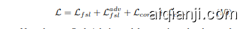
3.2. Style Extraction from CNNs and ViTs
3.2. 从CNN和ViT中提取风格
Adaptive Instance Normalization (AdaIN). We recap the vanilla AdaIN [22] proposed for CNN in style transfer. Particularly, AdaIN reveals that the instance-level mean and standard deviation (abbreviated as mean and std) convey the style information of the input image. Denoting the mean and std as $\mu$ and $\sigma$ , AdaIN (denoted as $\mathcal{A}$ ) reveals that the style of $F$ can be transfered to that of $F_{t g t}$ by replacing the original style $(\mu,\sigma)$ with the target style $(\mu_{t g t},\sigma_{t g t})$ :
自适应实例归一化 (AdaIN)。我们回顾了为风格迁移提出的CNN基础AdaIN方法[22]。具体而言,AdaIN揭示了实例级均值(mean)和标准差(std)承载着输入图像的风格信息。将均值与标准差记为$\mu$和$\sigma$,AdaIN(记作$\mathcal{A}$)表明:通过将原始风格$(\mu,\sigma)$替换为目标风格$(\mu_{t g t},\sigma_{t g t})$,可将$F$的风格迁移至$F_{t g t}$:

Style Extraction for CNN Features. As shown in the upper part of Figure 1 (b), let $\boldsymbol{F}\in\mathcal{R}^{B\times C\times H\times W}$ indicates the input feature batch, where $B,C,H$ , and $W$ denote the batch size, channel, height, and width of the feature $F$ , respectively. As in AdaIN, the mean $\mu$ and std $\sigma$ of $F$ are defined as:
CNN特征风格提取。如图1(b)上半部分所示,设$\boldsymbol{F}\in\mathcal{R}^{B\times C\times H\times W}$表示输入特征批次,其中$B,C,H$和$W$分别表示特征$F$的批次大小、通道数、高度和宽度。与AdaIN类似,$F$的均值$\mu$和标准差$\sigma$定义为:

where $\mu,\sigma\in\mathcal{R}^{B\times C}$ .
其中 $\mu,\sigma\in\mathcal{R}^{B\times C}$。
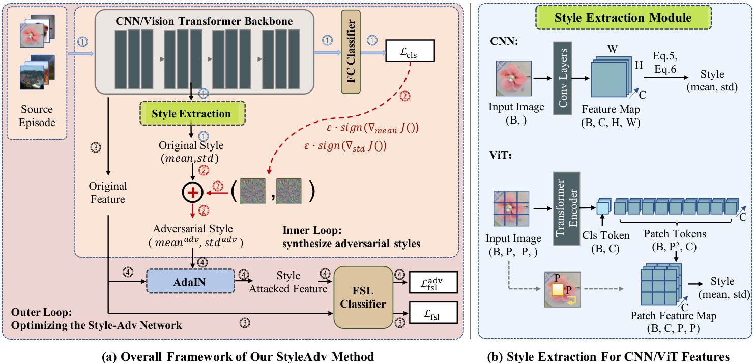
Figure 1. (a): Overview of StyleAdv method. The inner loop synthesizes adversarial styles, while the outer loop optimizes the whole network. (b): Style extraction for CNN-based and ViT-based features (illustration with $\scriptstyle\mathrm{B=1}$ ).
图 1: (a) StyleAdv方法概述。内循环合成对抗风格,外循环优化整个网络。(b) 基于CNN和ViT特征的风格提取 (以 $\scriptstyle\mathrm{B=1}$ 为例)。
Meta Information Extraction for ViT Features. We explore extracting the meta information of the ViT features as the manner of CNN. Intuitively, such meta information can be regarded as a unique “style” of ViTs. As shown in Figure 1 (b), we take an input batch data with image split into $P\times P$ patches as an example. The ViT encoder will encode the batch patches into a class (cls) token $(F_{c l s}\in\mathcal{R}^{B\times C})$ and a patch tokens $(F_{0}\in\mathcal{R}^{B\times P^{2}\times C})$ . To be compatible with AdaIN, we reshape the $F_{0}$ as $\boldsymbol{F}\in\mathcal{R}^{B\times C\times P\times P}$ . At this point, we can calculate the meta information for patch tokens $F$ as in Eq. 5 and Eq. 6. Essentially, note that the transformer integrates the positional embedding into the patch representation, the spatial relations thus could be considered still hold in the patch tokens. This supports us to reform the patch tokens $F_{0}$ as a spatial feature map $F$ . To some extent, this can also be achieved by applying the convolution on the input data via a kernel of size $P\times P$ (as indicated by dashed arrows in Figure 1 (b)).
ViT特征的元信息提取。我们探索以CNN的方式提取ViT特征的元信息。直观上,这类元信息可视为ViT独有的"风格"。如图1(b)所示,我们以输入批次数据(图像分割为$P\times P$块)为例,ViT编码器会将批次块编码为类别(cls)token$(F_{c l s}\in\mathcal{R}^{B\times C})$和块token$(F_{0}\in\mathcal{R}^{B\times P^{2}\times C})$。为兼容AdaIN,我们将$F_{0}$重塑为$\boldsymbol{F}\in\mathcal{R}^{B\times C\times P\times P}$。此时可按式5和式6计算块token$F$的元信息。本质上,由于transformer将位置嵌入整合到块表示中,空间关系仍可认为保留在块token中,这支持我们将块token$F_{0}$重构为空间特征图$F$。某种程度上,这也可通过在输入数据上应用$P\times P$核的卷积实现(如图1(b)虚线箭头所示)。
3.3. Inner Loop: Style Adversarial Attack Method
3.3. 内循环:风格对抗攻击方法
We propose a novel style adversarial attack method – Fast Style Gradient Sign Method (Style-FGSM) to accomplish the inner loop. As shown in Figure 1, given an input source episode $(T,Y)$ , we first forward it into the backbone $E$ and the FC classifier $f_{c l s}$ producing the global classification loss $\mathcal{L}{c l s}$ (as illustrated in the $\textcircled{1}$ paths). During this process, a key step is to make the gradient of the style available. To achieve that, let $F{T}$ denotes the features of $\tau$ , we obtain the style $(\mu,\sigma)$ of $F_{T}$ as in Sec. 3.2. After that, we reform the original episode feature as $\mathcal{A}(F_{\mathcal{T}},\mu,\sigma)$ . And the reformed feature is actually used for the forward propagation. In this way, we include $\mu$ and $\sigma$ in our forward computation chain; and thus, we could access the gradients of them.
我们提出了一种新颖的风格对抗攻击方法——快速风格梯度符号法 (Style-FGSM) 来实现内循环。如图 1 所示,给定输入源片段 $(T,Y)$,我们首先将其传入主干网络 $E$ 和全连接分类器 $f_{c l s}$ 以生成全局分类损失 $\mathcal{L}{c l s}$(如 $\textcircled{1}$ 路径所示)。在此过程中,关键步骤是使风格梯度可用。为此,令 $F{T}$ 表示 $\tau$ 的特征,我们按照第 3.2 节所述获取 $F_{T}$ 的风格 $(\mu,\sigma)$。之后,我们将原始片段特征重构为 $\mathcal{A}(F_{\mathcal{T}},\mu,\sigma)$,而重构后的特征实际用于前向传播。通过这种方式,我们将 $\mu$ 和 $\sigma$ 纳入前向计算链中,从而能够获取它们的梯度。
With the gradients in $\textcircled{2}$ paths, we then attack $\mu$ and $\sigma$ as FGSM does – adding a small ratio $\epsilon$ of the signed gradients with respect to $\mu$ and $\sigma$ , respectively.
通过 $\textcircled{2}$ 路径中的梯度,我们像FGSM那样对 $\mu$ 和 $\sigma$ 发起攻击——分别添加一个与 $\mu$ 和 $\sigma$ 相关的带符号梯度的小比例 $\epsilon$。

where the $J(\u)$ is the cross-entropy loss between classification predictions and ground truth $Y$ , i.e., $\mathcal{L}{c l s}$ . Inspired by the random start of PGD, we also add random noises $k{R T}\cdot\mathcal{N}(0,I)$ to $\mu$ and $\sigma$ before attacking. $\mathcal{N}(0,I)$ refers to Gaussian noises and $k_{R T}$ is a hyper-parameter. Our Style-FGSM enables us to generate both “virtual” and “hard” styles.
其中 $J(\u)$ 是分类预测与真实标签 $Y$ 之间的交叉熵损失,即 $\mathcal{L}{c l s}$。受PGD随机初始化的启发,我们在攻击前向 $\mu$ 和 $\sigma$ 添加随机噪声 $k{R T}\cdot\mathcal{N}(0,I)$。$\mathcal{N}(0,I)$ 表示高斯噪声,$k_{R T}$ 为超参数。我们的Style-FGSM能够生成"虚拟"和"硬"两种风格。
Progressive Style Synthesizing Strategy: To prevent the high-level adversarial feature from deviating, we propose to apply our style-FGSM in a progressive strategy. Concretely, the embedding module $E$ has three blocks $E_{1},E_{2}$ , and $E_{3}$ , with the corresponding features $F_{1}$ , $F_{2}$ , and $F_{3}$ . For the first block, we use $(\mu_{1},\sigma_{1})$ to denote the original styles of $F_{1}$ . The adversarial styles $(\mu_{1}^{a d v},\sigma_{1}^{a d v})$ are obtained directly as in Eq. 7 and Eq. 8. For subsequent blocks, the attack signals on the current block $i$ are those accumulated from the block 1 to block $i-1$ . Take the second block as an example, the block feature $F_{2}$ is not simply extracted by $E_{2}(F_{1})$ . Instead, we have $F_{2}^{'}=E_{2}(F_{1}^{a\bar{d}v\bar{}})$ , where $F_{1}^{a d v}=\mathcal{A}(F_{1},\mu_{1}^{a d v},\sigma_{1}^{a d v})$ . Attacking on $F_{2}^{'}$ results in the adversarial styles $(\mu_{2}^{a d v},\sigma_{2}^{a d v})$ . Accordingly, we generate $(\mu_{3}^{a d v},\sigma_{3}^{a d v})$ for the last block. The illustration of the progressive attacking strategy is attached in the Appendix.
渐进式风格合成策略:为防止高级对抗特征偏离,我们提出以渐进策略应用风格-FGSM。具体而言,嵌入模块 $E$ 包含三个块 $E_{1},E_{2}$ 和 $E_{3}$,对应特征为 $F_{1}$、$F_{2}$ 和 $F_{3}$。对于第一个块,使用 $(\mu_{1},\sigma_{1})$ 表示 $F_{1}$ 的原始风格,其对抗风格 $(\mu_{1}^{a d v},\sigma_{1}^{a d v})$ 直接通过式7和式8获得。对于后续块,当前块 $i$ 的攻击信号是从块1到块 $i-1$ 累积的。以第二块为例,块特征 $F_{2}$ 并非简单通过 $E_{2}(F_{1})$ 提取,而是通过 $F_{2}^{'}=E_{2}(F_{1}^{a\bar{d}v\bar{}})$ 获得,其中 $F_{1}^{a d v}=\mathcal{A}(F_{1},\mu_{1}^{a d v},\sigma_{1}^{a d v})$。对 $F_{2}^{'}$ 进行攻击得到对抗风格 $(\mu_{2}^{a d v},\sigma_{2}^{a d v})$,同理生成最后块的 $(\mu_{3}^{a d v},\sigma_{3}^{a d v})$。渐进攻击策略示意图见附录。
Changing Style Perturbation Ratios: Different from the vanilla FGSM [14] or PGD [34], our style attacking algorithm is expected to synthesize new styles with diversity. Thus, instead of using a fixed attacking ratio $\epsilon$ , we randomly sample $\epsilon$ from a candidate list $\epsilon_{l i s t}$ as the current attacking ratio. Despite the randomness of $\epsilon$ , we still synthesize styles in a more challenging direction, $\epsilon$ only affects the extent.
改变风格扰动比例:与原始FGSM [14] 或 PGD [34] 不同,我们的风格攻击算法旨在合成具有多样性的新风格。因此,我们不使用固定的攻击比例 $\epsilon$,而是从候选列表 $\epsilon_{list}$ 中随机采样 $\epsilon$ 作为当前攻击比例。尽管 $\epsilon$ 具有随机性,我们仍会沿更具挑战性的方向合成风格,$\epsilon$ 仅影响扰动程度。
3.4. Outer Loop: Optimize the StyleAdv Network
3.4. 外循环:优化StyleAdv网络
For each meta-train iteration with clean episode $\tau$ as input, our inner loop produces adversarial styles $(\mu_{1}^{a d v},\sigma_{1}^{a d v})$ , $(\mu_{2}^{a d v},\sigma_{2}^{a d v})$ , and $(\mu_{3}^{a d v},\sigma_{3}^{a d v})$ . As in Figure 1, the goal of the outer loop is to optimize the whole StyleAdv with both the clean feature $F$ and the style attacked feature $F^{a d v}$ utilized as the training data. Typically, the clean episode feature $F$ can be obtained directly as $E(\mathcal{T})$ as in $\textcircled{3}$ paths.
对于每个以干净片段$\tau$作为输入的元训练迭代,我们的内循环会生成对抗风格$(\mu_{1}^{a d v},\sigma_{1}^{a d v})$、$(\mu_{2}^{a d v},\sigma_{2}^{a d v})$和$(\mu_{3}^{a d v},\sigma_{3}^{a d v})$。如图1所示,外循环的目标是通过同时利用干净特征$F$和风格攻击特征$F^{a d v}$作为训练数据,来优化整个StyleAdv。通常,干净片段特征$F$可以直接通过$\textcircled{3}$路径中的$E(\mathcal{T})$获得。
In $\textcircled{4}$ paths, we obtain the $F^{a d v}$ by transferring the original style of $F$ to the corresponding adversarial attacked styles. Similar with the progressive style-FGSM, we have F 1adv $F_{1}^{a d v}={\cal A}(E_{1}(T),\mu_{1}^{a d v},\sigma_{1}^{a d v})$ , $\begin{array}{r l r}{F_{2}^{a d v}}&{{}=}&{{\cal A}(E_{2}({F_{1}^{a d v}}),\mu_{2}^{a d v},\sigma_{2}^{a d v})}\end{array}$ , aTnd $F_{3}^{a d v}=$ $\mathcal{A}(E_{3}(F_{2}^{a d v}),\mu_{3}^{a d v},\sigma_{3}^{a d v})$ . Finally, $F^{a d v}$ is obtained by applying an average pooling layer to $F_{3}^{a d v}$ . A skip probability $p_{s k i p}$ is set to decide whether to skip the current attacking. Conducting FSL tasks for both the clean feature $F$ and style attacked feature $F^{a d v}$ results in two FSL predictions $P_{f s l}$ , $P_{f s l}^{a d v}$ , and two FSL classification losses $\mathcal{L}_{f s l},\mathcal{L}_{f s l}^{a d v}$ .
在 $\textcircled{4}$ 路径中,我们通过将 $F$ 的原始风格转换为相应的对抗攻击风格来获得 $F^{a d v}$。与渐进式风格-FGSM类似,我们有 $F_{1}^{a d v}={\cal A}(E_{1}(T),\mu_{1}^{a d v},\sigma_{1}^{a d v})$、$\begin{array}{r l r}{F_{2}^{a d v}}&{{}=}&{{\cal A}(E_{2}({F_{1}^{a d v}}),\mu_{2}^{a d v},\sigma_{2}^{a d v})}\end{array}$,以及 $F_{3}^{a d v}=$ $\mathcal{A}(E_{3}(F_{2}^{a d v}),\mu_{3}^{a d v},\sigma_{3}^{a d v})$。最终,通过对 $F_{3}^{a d v}$ 应用平均池化层得到 $F^{a d v}$。设定跳过概率 $p_{s k i p}$ 来决定是否跳过当前攻击。对干净特征 $F$ 和风格攻击特征 $F^{a d v}$ 执行少样本学习 (FSL) 任务,得到两个 FSL 预测 $P_{f s l}$、$P_{f s l}^{a d v}$ 和两个 FSL 分类损失 $\mathcal{L}_{f s l},\mathcal{L}_{f s l}^{a d v}$。
Further, despite the styles of $F^{a d v}$ shifts from that of $F$ , we encourage that the semantic content should be still consistent as in wave-SAN [10]. Thus we add a consistent constraint to the predictions of $P_{f s l}$ and $P_{f s l}^{a d v}$ resulting in the consistent loss Lcons as,
此外,尽管 $F^{a d v}$ 的风格与 $F$ 不同,我们仍鼓励其语义内容应保持与 wave-SAN [10] 一致。因此,我们在 $P_{f s l}$ 和 $P_{f s l}^{a d v}$ 的预测中添加了一致性约束,从而得到一致性损失 $L_{cons}$,其表达式为:

where $\mathrm{KL()}$ is Kullback–Leibler divergence loss. In addition, we have the global classification loss $\mathcal{L}{c l s}$ . This ensures that $\theta{c l s}$ is optimized to provide correct gradients for styleFGSM. The final meta-objective of StyleAdv is as,
其中 $\mathrm{KL()}$ 是 Kullback-Leibler 散度损失。此外,我们还引入了全局分类损失 $\mathcal{L}{cls}$ ,以确保 $\theta{cls}$ 经过优化后能为 styleFGSM 提供正确的梯度。StyleAdv 的最终元目标如下:
Note that our StyleAdv is model-agnostic and orthogonal to existing FSL and CD-FSL methods.
请注意,我们的StyleAdv与模型无关,且与现有的FSL和CD-FSL方法正交。
3.5. Network Inference
3.5. 网络推断
Applying StyleAdv Directly for Inference. Our StyleAdv facilitates making CD-FSL model more robust to style shifts. Once the model is meta-trained, we can employ it for inference directly by feeding the testing episode into the $E$ and the $f_{c l s}$ . The class with the highest probability will be taken as the predicted result.
直接应用StyleAdv进行推理。我们的StyleAdv能够提升CD-FSL模型对风格变化的鲁棒性。当模型完成元训练后,只需将测试片段输入$E$和$f_{cls}$即可直接用于推理。概率最高的类别将被作为预测结果。
Finetuning StyleAdv Using Target Examples. As indicated in previous works [16, 32, 33, 51], finetuning CD-FSL models on target examples helps improve the model performance. Thus, to further promote the performance of StyleAdv, we also equip it with the fintuning strategy forming an upgraded version (“StyleAdv-FT”). Specifically, as in ATA-FT [51], for each novel testing episode, we augment the novel support set to form pseudo episodes as training data for tuning the meta-trained model.
使用目标样本微调StyleAdv。如先前研究[16, 32, 33, 51]所述,在目标样本上微调跨域小样本学习(CD-FSL)模型有助于提升性能。因此,我们为StyleAdv引入微调策略,形成升级版本("StyleAdv-FT")。具体实现参照ATA-FT[51]:针对每个新测试任务,通过扩增新支持集构建伪训练任务,用于调整元训练后的模型。
4. Experiments
4. 实验
Datasets. We take two CD-FSL benchmarks proposed in BSCD-FSL [16] and FWT [48]. Both of them take miniImagenet [39] as the source dataset. Two disjoint sets split from mini-Imagenet form $\mathcal{D}^{t r}$ and $\mathcal{D}^{e v a l}$ . Totally eight datasets including ChestX [53], ISIC [4, 47], EuroSAT [18], CropDisease [35], CUB [50], Cars [24], Places [64], and Plantae [49] are taken as novel target datasets. The former four datasets included in BSCD-FSL’s benchmark cover medical images varying from X-ray to der mos co pic skin lesions, and natural images from satellite pictures to plant disease photos. While the latter four datasets that focus on more fine-grained concepts such as birds and cars are contained in FWT. These eight target datasets serve as testing set $\mathcal{D}^{t e}$ , respectively.
数据集。我们采用BSCD-FSL[16]和FWT[48]提出的两个跨域小样本学习(CD-FSL)基准。两者均以miniImagenet[39]作为源数据集,通过划分mini-Imagenet形成互斥的训练集$\mathcal{D}^{tr}$和验证集$\mathcal{D}^{eval}$。共采用八个新颖目标数据集:ChestX[53]、ISIC[4,47]、EuroSAT[18]、CropDisease[35]、CUB[50]、Cars[24]、Places[64]和Plantae[49]。其中BSCD-FSL基准包含前四个数据集,涵盖从X光片到皮肤镜图像的医学影像,以及从卫星图像到植物病害照片的自然图像;而FWT则包含后四个专注于细粒度概念(如鸟类和汽车)的数据集。这八个目标数据集分别作为测试集$\mathcal{D}^{te}$。
Network Modules. For typical CNN based network, following previous CD-FSL methods [10, 42, 48, 51], ResNet10 [17] is selected as the embedding module while GNN [12] is selected as the FSL classifier; For the emerging ViT based network, following PMF [19], we use the ViT-small [5] and the ProtoNet [41] as the embedding module and the FSL classifier, respectively. Note that, the ViT-small is pretrained on ImageNet1K by DINO [2] as in PMF. The $f_{c l s}$ is built by a fully connected layer.
网络模块。对于典型的基于CNN的网络,遵循先前CD-FSL方法[10, 42, 48, 51],选择ResNet10[17]作为嵌入模块,GNN[12]作为FSL分类器;对于新兴的基于ViT的网络,遵循PMF[19],我们分别使用ViT-small[5]和ProtoNet[41]作为嵌入模块和FSL分类器。需要注意的是,ViT-small通过DINO[2]在ImageNet1K上进行预训练,与PMF中一致。$f_{cls}$通过一个全连接层构建。
Implementation Details. The 5-way 1-shot and 5-way 5- shot settings are conducted. Taking ResNet10 as backbone, we meta train the network for 200 epochs, each epoch contains 120 meta tasks. Adam with a learning rate of 0.001 is utilized as the optimizer. Taking ViT-small as backbone, the meta train stage takes 20 epoch, each epoch contains 2000 meta tasks. The SGD with a initial learning rate of 5e-5 and 0.001 are used for optimize the $E()$ and the $f_{c l s}$ , respectively. The ${\epsilon_{l i s t}}$ , $k_{R T}$ of Style-FGSM attacker are set as [0.8, 0.08, 0.008], 21565 . The probability $p_{s k i p}$ of random skipping the attacking is chosen from ${0.2,0.4}$ . We evaluate our network with 1000 randomly sampled episodes and report average accuracy $(%)$ with a $95%$ confidence interval. Both the results of our “StyleAdv” and “StyleAdv-FT” are reported. The details of the finetuning are attached in Appendix. ResNet-10 based models are trained and tested on a single GeForce GTX 1080, while ViT-small based models require a single NVIDIA GeForce RTX 3090.
实现细节。采用5-way 1-shot和5-way 5-shot设置。以ResNet10为骨干网络时,元训练进行200个周期,每个周期包含120个元任务,使用学习率为0.001的Adam优化器。以ViT-small为骨干网络时,元训练阶段进行20个周期,每个周期包含2000个元任务,分别采用初始学习率为5e-5和0.001的SGD优化器来优化$E()$和$f_{cls}$。Style-FGSM攻击者的${\epsilon_{list}}$和$k_{RT}$参数设置为[0.8, 0.08, 0.008]和21565。随机跳过攻击的概率$p_{skip}$从${0.2,0.4}$中选取。我们在1000个随机采样的测试片段上评估网络性能,并报告平均准确率$(%)$及其95%置信区间。"StyleAdv"和"StyleAdv-FT"的结果均被记录,微调细节见附录。基于ResNet-10的模型在单块GeForce GTX 1080上训练测试,基于ViT-small的模型需使用单块NVIDIA GeForce RTX 3090。
Table 1. Results of 5-way 1-shot/5-shot tasks. “FT” means whether the finetuning stage is employed. “LargeP”’ represents if large pretrained models are used for model initialization. “RN10” is short for “ResNet $10^{\ '}$ . $^*$ denotes results are reported by us. Results perform best are bolded. Whether based on ResNet-10 or ViT-small, our method outperforms other competitors significantly.
表 1: 5-way 1-shot/5-shot任务结果。"FT"表示是否采用微调阶段。"LargeP"代表是否使用大规模预训练模型进行初始化。"RN10"是"ResNet $10^{\ '}$"的缩写。$^*$表示结果由我们复现。最佳结果以粗体显示。无论基于ResNet-10还是ViT-small,我们的方法均显著优于其他竞争者。
| 1-shot | Backbone | FT | LargeP | ChestX | ISIC | EuroSAT | CropDisease | CUB | Cars | Places | Plantae | Average |
|---|---|---|---|---|---|---|---|---|---|---|---|---|
| GNN [12] | RN10 | 22.00±0.46 | 32.02±0.66 | 63.69±1.03 | 64.48±1.08 | 45.69±0.68 | 31.79±0.51 | 53.10±0.80 | 35.60±0.56 | 43.55 | ||
| FWT [48] | RN10 | 22.04±0.44 | 31.58±0.67 | 62.36±1.05 | 66.36±1.04 | 47.47±0.75 | 31.61±0.53 | 55.77±0.79 | 35.95±0.58 | 44.14 | ||
| LRP [42] | RN10 | 22.11±0.20 | 30.94±0.30 | 54.99±0.50 | 59.23±0.50 | 48.29±0.51 | 32.78±0.39 | 54.83±0.56 | 37.49±0.43 | 42.58 | ||
| ATA [51] | RN10 | 22.10±0.20 33.21±0.40 | 61.35±0.50 | 67.47±0.50 | 45.00±0.50 | 33.61±0.40 | 53.57±0.50 | 34.42±0.40 | 43.84 | |||
| AFA [20] | RN10 | 22.92±0.20 33.21±0.30 | 63.12±0.50 | 67.61±0.50 | 46.86±0.50 | 34.25±0.40 | 54.04±0.60 | 36.76±0.40 | 44.85 | |||
| wave-SAN [10] | RN10 | 22.93±0.49 33.35±0.71 | 69.64±1.09 | 70.80±1.06 | 50.25±0.74 | 33.55±0.61 | 57.75±0.82 | 40.71±0.66 | 47.37 | |||
| StyleAdv (ours) | RN10 | - | 22.64±0.35 33.96±0.57 | 70.94±0.82 | 74.13±0.78 | 48.49±0.72 34.64±0.57 | 58.58±0.83 | 41.13±0.67 | 48.06 | |||
| ATA-FT [51] | RN10 | Y | 22.15±0.20 34.94±0.40 | 68.62±0.50 | 75.41±0.50 | 46.23±0.50 | 37.15±0.40 | 54.18±0.50 | 37.38±0.40 | 47.01 | ||
| StyleAdv-FT (ours) | RN10 | Y | 22.64±0.35 | 35.76±0.52 | 72.92±0.75 | 80.69±0.28 | 48.49±0.72 | 35.09±0.55 | 58.58±0.83 | 41.13±0.67 | 49.41 | |
| PMF* [19] | ViT-small | Y | DINO/IN1K | 21.73±0.30 | 30.36±0.36 | 70.74±0.63 | 80.79±0.62 | 78.13±0.66 | 37.24±0.57 | 71.11±0.71 | 53.60±0.66 | 55.46 |
| StyleAdv (ours) | ViT-small | DINO/IN1K | 22.92±0.32 | 33.05±0.44 | 72.15±0.65 | 81.22±0.61 | 84.01±0.58 | 40.48±0.57 | 72.64±0.67 | 55.52±0.66 | 57.75 | |
| StyleAdv-FT (ours) | ViT-small | Y | DINO/IN1K | 22.92±0.32 | 33.99±0.46 | 74.93±0.58 | 84.11±0.57 | 84.01±0.58 | 40.48±0.57 | 72.64±0.67 | 55.52±0.66 | 58.57 |
| 5-shot | Backbone | FT | LargeP | ChestX | ISIC | EuroSAT | CropDisease | CUB | Cars | Places | Plantae | Average |
|---|---|---|---|---|---|---|---|---|---|---|---|---|
| GNN [12] | RN10 | 25.27±0.46 | 43.94±0.67 | 83.64±0.77 | 87.96±0.67 | 62.25±0.65 | 44.28±0.63 | 70.84±0.65 | 52.53±0.59 | 58.84 | ||
| FWT [48] | RN10 | = | 25.18±0.45 43.17±0.70 | 83.01±0.79 | 87.11±0.67 | 66.98±0.68 | 44.90±0.64 | 73.94±0.67 | 53.85±0.62 | 59.77 | ||
| LRP [42] | RN10 | 24.53±0.30 44.14±0.40 | 77.14±0.40 | 86.15±0.40 | 64.44±0.48 | 46.20±0.46 | 74.45±0.47 | 54.46±0.46 | 58.94 | |||
| ATA [51] | RN10 | 24.32±0.40 44.91±0.40 83.75±0.40 | 90.59±0.30 | 66.22±0.50 | 49.14±0.40 | 75.48±0.40 | 52.69±0.40 | 60.89 | ||||
| AFA [20] | RN10 | 25.02±0.20 46.01±0.40 | 85.58±0.40 | 88.06±0.30 | 68.25±0.50 | 49.28±0.50 | 76.21±0.50 | 54.26±0.40 | 61.58 | |||
| wave-SAN [10] | RN10 | 25.63±0.49 44.93±0.67 | 785.22±0.71 | 89.70±0.64 | 70.31±0.67 | 46.11±0.66 | 76.88±0.63 | 57.72±0.64 | 62.06 | |||
| StyleAdv (ours) | RN10 | = | 26.07±0.37 45.77±0.51 86.58±0.54 | 93.65±0.39 | 68.72±0.67 | 50.13±0.68 | 77.73±0.62 | 61.52±0.68 | 63.77 | |||
| Fine-tune [16] | RN10 | Y | 25.97±0.41 48.11±0.64 | 79.08±0.61 | 89.25±0.51 | 64.14±0.77 | 52.08±0.74 | 70.06±0.74 | 59.27±0.70 | 61.00 | ||
| ATA-FT [51] | RN10 | 人 | 25.08±0.20 49.79±0.40 | 89.64±0.30 | 95.44±0.20 | 69.83±0.50 | 54.28±0.50 | 76.64±0.40 | 58.08±0.40 | 64.85 | ||
| NSAE [32] | RN10 | Y | 27.10±0.44 54.05±0.63 | 83.96±0.57 | 93.14±0.47 | 68.51±0.76 | 54.91±0.74 | 71.02±0.72 | 59.55±0.74 | 64.03 | ||
| BSR [33] | RN10 | 人 | 26.84±0.44 54.42±0.66 | 80.89±0.61 | 92.17±0.45 | 69.38±0.76 | 57.49±0.72 | 71.09±0.68 | 61.07±0.76 | 64.17 | ||
| StyleAdv-FT (ours) | RN10 | 人 | 26.24±0.35 53.05±0.54 | 91.64±0.43 | 96.51±0.28 | 70.90±0.63 | 56.44±0.68 | 79.35±0.61 | 64.10±0.64 | 67.28 | ||
| PMF [19] | ViT-small | Y | DINO/IN1K | 27.27 | 50.12 | 85.98 | 92.96 | |||||
| StyleAdv (ours) | ViT-small | DINO/IN1K | 26.97±0.33 | 47.73±0.44 | 88.57±0.34 | 94.85±0.31 | 95.82±0.27 | 61.73±0.62 | 88.33±0.40 | 75.55±0.54 | 72.44 | |
| StyleAdv-FT (ours) | ViT-small | Y | DINO/IN1K | 26.97±0.33 | 51.23±0.51 | 90.12±0.33 | 95.99±0.27 | 95.82±0.27 | 66.02±0.64 | 88.33±0.40 | 78.01±0.54 | 74.06 |
4.1. Comparison with the SOTAs
4.1. 与SOTA的对比
We compare our StyleAdv/StyleAdv-FT against several most representative and competitive CD-FSL methods. Concretly, with the ResNet-10 (abbreviated as RN10) as backbone, totally nine methods including GNN [12], FWT [48], LRP [42], ATA [51], AFA [20], wave-SAN [10], Finetune [16], NSAE [32], and BSR [33] are introduced as our competitors. Among them, the former six competitors are meta-learning based method that used for inference directly, thus we compare our “StyleAdv” against them for a fair comparison. Typically, the GNN [12] works as a base model. The Fine-tune [16], NSAE [32], BSR [33], and ATA-FT [51] (formed by finetuning ATA) all require finetuning model during inference, thus our “StyleAdv-FT” is used. With the ViT as backbone, the most recent and competitive PMF (SOTA method for FSL) is compared. For fair comparisons, we follow the same pipeline proposed in PMF [19]. Note that we promote CD-FSL models with only one single source domain. Those methods that use extra training datasets, e.g., STARTUP [37], meta-FDMixup [8], and DSL [21] are not considered. The comparison results are given in Table 1.
我们将StyleAdv/StyleAdv-FT与几种最具代表性和竞争力的跨域小样本学习(CD-FSL)方法进行对比。具体而言,以ResNet-10(缩写为RN10)为骨干网络时,共引入九种方法作为竞争对手:GNN [12]、FWT [48]、LRP [42]、ATA [51]、AFA [20]、wave-SAN [10]、Finetune [16]、NSAE [32]和BSR [33]。其中前六种是基于元学习的方法可直接用于推理,因此我们使用"StyleAdv"与之进行公平对比(GNN [12]作为基线模型)。而Finetune [16]、NSAE [32]、BSR [33]和通过微调ATA形成的ATA-FT [51]在推理时都需要微调模型,故采用我们的"StyleAdv-FT"进行对比。以ViT为骨干网络时,则与当前最先进的PMF(小样本学习SOTA方法)进行对比。为保证公平性,我们遵循PMF [19]提出的相同流程。需要注意的是,我们仅使用单一源域推进CD-FSL模型,因此未考虑那些使用额外训练数据集的方法(如STARTUP [37]、meta-FDMixup [8]和DSL [21])。对比结果如表1所示。
For all results, our method outperforms all the listed CD-FSL competitors significantly and builds a new state of the art. Our StyleAdv-FT (ViT-small) on average achieves $58.57%$ and $74.06%$ on 5-way 1-shot and 5-shot, respectively. Our StyleAdv (RN10) and StyleAdv-FT (RN10) also beats all the meta-learning based or transfer-learning (finetuning) based methods. Besides of the state-of-the-art accuracy, we also have other worth-mentioning observations. 1) We show that our StyleAdv method is a general solution for both CNN-based models and ViT-based models. Typically, based on ResNet10, our StyleAdv and StyleAdv-FT improve the base GNN by up to $4.93%$ and $8.44%$ on 5-shot setting. Based on ViT-small, at most cases, our StyleAdvFT outperforms the PMF by a clear margin. More results of building StyleAdv upon other FSL or CD-FSL methods can be found in the Appendix. 2) Comparing FWT, LRP, ATA, AFA, waveSAN, and our StyleAdv, we find that StyleAdv performs best, followed by wave-SAN, then comes the AFA, ATA, FWT, and LRP. This phenomenon indicates that tackling CD-FSL by solving the visual shift problem is indeed more effective than other perspectives, e.g., adversarial training by perturbing the image features (AFA) or image pixels (ATA), transforms the normalization layers in FWT, and explanation guided training in LRP. 3) For the comparison between StyleAdv and wave-SAN that both tackles the visual styles, we notice that StyleAdv outperforms the wave-SAN in most cases. This demonstrates that the styles generated by our StyleAdv are more conducive to learning robust CD-FSL models than the style augmentation method proposed in wave-SAN. This justifies our idea of synthesizing more challenging (“hard and virtual”) styles.
在所有结果中,我们的方法显著超越了所有列出的跨域小样本学习(CD-FSL)竞争对手,建立了新的技术标杆。我们的StyleAdv-FT (ViT-small)在5-way 1-shot和5-shot设置下平均分别达到$58.57%$和$74.06%$。StyleAdv (RN10)和StyleAdv-FT (RN10)同样优于所有基于元学习或迁移学习(微调)的方法。除了最先进的准确率外,我们还有其他值得关注的发现:1) StyleAdv方法对基于CNN和ViT的模型都具有普适性。基于ResNet10时,我们的方法在5-shot设置下将GNN基线最高提升了$4.93%$和$8.44%$;基于ViT-small时,StyleAdvFT在多数情况下明显优于PMF。更多将StyleAdv应用于其他FSL或CD-FSL方法的结果见附录。2) 对比FWT、LRP、ATA、AFA、waveSAN和我们的StyleAdv,性能排序为:StyleAdv > wave-SAN > AFA > ATA > FWT > LRP。这表明通过解决视觉偏移问题来处理CD-FSL,比对抗训练(扰动图像特征的AFA或扰动像素的ATA)、变换归一化层(FWT)和解释引导训练(LRP)等方法更有效。3) 在同样处理视觉风格的StyleAdv与wave-SAN对比中,StyleAdv在多数情况下表现更优,证明我们生成的"困难虚拟"风格比wave-SAN的风格增强方法更能促进鲁棒CD-FSL模型的学习。
- Overall, the large-scale pretrained model promotes the CD-FSL obviously. Take 1-shot as an example, StyleAdv-FT (ViT-small) boosts the StyleAdv-FT (RN10) by $9.16%$ on average. However, we show that the performance improvement varies greatly on different target domains. Generally, for target datasets with relative small domain gap, e.g., CUB and Plantae, models benefit a lot; otherwise, the improvement is limited. 5) We also find that under the cross-domain scenarios, finetuning model on target domain, e.g., NSAE, BSR do show an advantange over purely meta-learning based methods, e.g., FWT, LRP, and wave-SAN. However, to finetune model using extremely few examples, e.g., 5-way 1-shot is much harder than on relatively larger shots. This may explain why those finetune-based methods do not conduct experiments on 1-shot setting.
- 总体而言,大规模预训练模型显著提升了跨域小样本学习(CD-FSL)性能。以1-shot为例,StyleAdv-FT (ViT-small)平均比StyleAdv-FT (RN10)高出$9.16%$。但我们发现性能提升在不同目标域间差异显著:对于域差距较小的目标数据集(如CUB和Plantae),模型提升幅度较大;反之则提升有限。5) 我们还发现,在跨域场景下,基于目标域微调的方法(如NSAE、BSR)确实优于纯元学习方法(如FWT、LRP和wave-SAN)。但使用极少量样本(如5-way 1-shot)进行微调比使用较多shot更具挑战性,这可能是基于微调的方法未在1-shot设置下进行实验的原因。
Effectiveness of Style-FGSM Attacker. To show the advantages of our progressive style synthesizing strategy and attacking with changing perturbation ratios, we compare our Style-FGSM against several variants and report the results in Figure 2. Specifically, for Figure 2 (a), we compare our styleFGSM against the variant that attacks the blocks individually. Results show that attacking in a progressive way exceeds the naive individual strategy in most cases. For Figure 2 (b), to demonstrate how the performance will be affected by fixed attacking ratios, we also conduct experiments with different $\epsilon_{l i s t}$ . Since we set the $\epsilon_{l i s t}$ as [0.8, 0.08, 0.008], three different choices including [0.8], [0.08], and [0.008] are selected. From the results, we first notice that the best result can be reached by a single fixed ratio. However, sampling the attacking ratio from a pool of candidates achieves the best result in most cases.
Style-FGSM攻击器的有效性。为展示我们渐进式风格合成策略及动态扰动比例攻击的优势,我们将Style-FGSM与多个变体进行对比,结果如图2所示。具体而言,在图2(a)中,我们将styleFGSM与逐个模块攻击的变体进行比较。结果表明,渐进式攻击在多数情况下优于简单的独立攻击策略。对于图2(b),为展示固定攻击比例对性能的影响,我们采用不同$\epsilon_{list}$进行实验。由于设置$\epsilon_{list}$为[0.8, 0.08, 0.008],我们选取了[0.8]、[0.08]和[0.008]三种不同配置。结果显示,虽然单一固定比例可获得最佳结果,但从候选比例池中采样攻击比例在多数情况下表现最优。

Figure 2. Effectiveness of the progressive style synthesizing strategy and the changing style perturbation ratios. The 5-way 1-shot results are reported. Models are built on ResNet10 and GNN.
图 2: 渐进式风格合成策略及动态风格扰动比例的有效性。实验结果为5-way 1-shot场景,模型基于ResNet10和GNN构建。
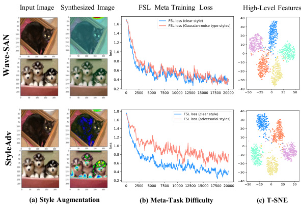
Figure 3. Visualization of wave-SAN and StyleAdv. (a): synthesized images; (b): meta-training losses; (c): T-SNE results.
图 3: wave-SAN 和 StyleAdv 的可视化效果。(a): 合成图像; (b): 元训练损失; (c): T-SNE 结果。
4.2. More Analysis
4.2. 更多分析
Visualization of Hard Style Generation. To help understand the “hard” style generation of our method intuitively, as in Figure 3, we make several visualization s comparing StyleAdv against the wave-SAN. 1) As in Figure 3 (a), we show the stylized images generated by wave-SAN and our StyleAdv. The visualization is achieved by applying the style augmentation methods to input images. Specifically, for wave-SAN, the style is swapped with another randomly sampled source image; for StyleAdv, the results of attacking style with $\epsilon=0.08$ are given. We observe that wave-SAN tends to exchange the global visual appearance, e.g., the color of the input image randomly. By contrast, StyleAdv prefers to disturb the important regions that are key to recognizing the image category. For example, the fur of the cat and the key parts (face and feet) of the dogs. These observations intuitively support our claim that our StyleAdv synthesize more harder styles than wave-SAN. 2) To quantitatively evaluate whether our StyleAdv introduces more challenging styles into the training stage, as in Figure 3 (b), we visualize the meta-training loss. Results reveal that the perturbed losses of wave-SAN oscillate around the original loss, while StyleAdv increases the original loss obviously. These phenomenons further validate that we perturb data towards a more difficult direction thus pushing the limits of style generation to a large extent. 3) To further show the advantages of StyleAdv over wave-SAN, as shown in Figure 3 (c), we visualize the high-level features extracted by the meta-trained wave-SAN and StyleAdv. Five classes (denoted by different colors) of mini-Imagenet are selected. T-SNE is used for reducing the feature dimensions. Results demonstrate that StyleAdv enlarges the inter-class distances making classes more distinguishable.
硬风格生成可视化。为直观理解本方法的"硬"风格生成机制,如图3所示,我们通过多组可视化对比StyleAdv与wave-SAN:1) 图3(a)展示wave-SAN与StyleAdv生成的风格化图像,通过对输入图像施加风格增强方法实现可视化。具体而言,wave-SAN将风格替换为随机采样的源图像;StyleAdv则呈现攻击强度$\epsilon=0.08$时的风格扰动结果。可观察到wave-SAN倾向于随机改变全局视觉特征(如图像色调),而StyleAdv更侧重干扰图像类别识别的关键区域(如猫的毛发、狗的面部与足部),直观佐证了StyleAdv能合成更难风格的论点。2) 为定量评估StyleAdv是否在训练阶段引入更具挑战性的风格,图3(b)可视化元训练损失曲线。结果显示wave-SAN的扰动损失围绕原始损失波动,而StyleAdv显著提升了原始损失值,这种现象进一步验证了我们通过数据扰动实现了更困难的风格生成方向。3) 图3(c)通过t-SNE降维可视化wave-SAN与StyleAdv提取的高维特征(选用mini-Imagenet中五类不同颜色标注的数据),表明StyleAdv能扩大类间距离从而提升特征可分性。
Why Attack Styles Instead of Images or Features? A natural question may be why we choose to attack styles instead of other targets, e.g., the input image as in AQ [13], MDAT [30], and ATA [51] or the features as in Shen et al. [40] and AFA [20]? To answer this question, we compare our StyleAdv which attacks styles against attacking images and features by modifying the attack targets of our method. The 5-way 1-shot/5-shot results are given in Table 2. We highlight several points. 1) We notice that attacking image, feature, and style all improve the base GNN model (given in Table 1) which shows that all of them boost the generalization ability of the model by adversarial attacks. Interestingly, the results of our “Attack Image”/“Attack Feature” even outperform the well-designed CD-FSL methods ATA [51] and AFA [20] (shown in Table 1); 2) Our method has clear advantages over attacking images and features. This again indicates the superiority of tackling visual styles for narrowing the domain gap issue for CD-FSL.
为何攻击风格而非图像或特征?
一个自然的问题是,为何我们选择攻击风格而非其他目标,例如AQ [13]、MDAT [30]和ATA [51]中攻击输入图像,或Shen等人[40]与AFA [20]中攻击特征?为回答此问题,我们通过修改本方法的攻击目标,将攻击风格的StyleAdv与攻击图像和特征的方法进行对比。5-way 1-shot/5-shot结果如表2所示。我们强调以下几点:
- 注意到攻击图像、特征和风格均提升了基础GNN模型(见表1),表明它们都能通过对抗攻击增强模型的泛化能力。有趣的是,本研究的“攻击图像”/“攻击特征”结果甚至优于精心设计的CD-FSL方法ATA [51]和AFA [20](见表1);
- 本方法较攻击图像和特征具有明显优势,再次表明通过处理视觉风格来解决CD-FSL领域差距问题的优越性。
表2:
Table 3. Different style augmentation methods are compared. “StyleGaus†” means adding random Gaussian noises to the styles, where represents it is proposed by us. “MixStyle [66]”, “AdvStyle [63]” and “DSU [31]” are adapted from other tasks, e.g., domain generation. Results $(%)$ conducted under 5-way 1-shot/5-shot settings. Methods are built upon the ResNet10 and GNN.
| 攻击目标 | ChestX | ISIC | EuroSAT | CropDisease | CUB | Cars | Places | Plantae | 平均 | |
|---|---|---|---|---|---|---|---|---|---|---|
| 1-shot | 图像 | 22.71±0.35 | 33.00±0.53 | 67.00±0.82 | 72.65±0.75 | 48.15±0.72 | 34.40±0.60 | 57.89±0.83 | 39.85±0.64 | 46.96 |
| 特征 | 22.55±0.35 | 32.95±0.53 | 68.71±0.81 | 70.86±0.78 | 46.52±0.70 | 34.07±0.54 | 56.68±0.81 | 39.62±0.62 | 46.50 | |
| 风格(本文) | 22.64±0.35 | 33.96±0.57 | 70.94±0.82 | 74.13±0.78 | 48.49±0.72 | 34.64±0.57 | 58.58±0.83 | 41.13±0.67 | 48.06 | |
| 5-shot | 图像 | 24.92±0.36 | 42.63±0.47 | 84.18±0.54 | 90.31±0.47 | 66.37±0.65 | 47.46±0.67 | 75.94±0.62 | 57.33±0.65 | 61.14 |
| 特征 | 25.55±0.37 | 43.71±0.50 | 84.22±0.55 | 91.71±0.44 | 67.31±0.67 | 50.26±0.67 | 76.46±0.65 | 57.39±0.63 | 62.08 | |
| 风格(本文) | 26.07±0.37 | 45.77±0.51 | 86.58±0.54 | 93.65±0.39 | 68.72±0.67 | 50.13±0.68 | 77.73±0.62 | 61.52±0.68 | 63.77 |
| 增强方法 | ChestX | ISIC | EuroSAT | CropDisease | CUB | Cars | Places | Plantae | 平均 | |
|---|---|---|---|---|---|---|---|---|---|---|
| 1-shot | StyleGaus† | 22.37±0.35 | 31.48±0.52 | 65.71±0.82 | 69.25±0.80 | 46.32±0.72 | 32.69±0.54 | 55.48±0.79 | 37.27±0.61 | 45.07 |
| MixStyle [66] | 22.43±0.35 | 33.21±0.53 | 67.35±0.80 | 68.80±0.82 | 47.08±0.73 | 33.39±0.58 | 56.12±0.78 | 38.03±0.62 | 45.80 | |
| AdvStyle [63] | 22.04±0.36 | 30.83±0.52 | 65.19±0.82 | 64.96±0.81 | 47.43±0.72 | 31.90±0.52 | 53.95±0.79 | 35.81±0.59 | 44.01 | |
| DSU [31] | 22.35±0.36 | 31.43±0.51 | 64.55±0.83 | 64.73±0.81 | 47.74±0.72 | 31.61±0.53 | 54.81±0.81 | 37.19±0.61 | 44.30 | |
| Style-FGSM(本文) | 22.64±0.35 | 33.96±0.57 | 70.94±0.82 | 74.13±0.78 | 48.49±0.72 | 34.64±0.57 | 58.58±0.83 | 41.13±0.67 | 48.06 | |
| 5-shot | StyleGaus† | 24.97±0.37 | 41.74±0.48 | 81.88±0.61 | 89.71±0.49 | 65.98±0.67 | 45.03±0.64 | 72.66±0.68 | 56.66±0.65 | 59.83 |
| MixStyle [66] | 25.04±0.36 | 43.77±0.53 | 82.67±0.58 | 88.90±0.52 | 65.73±0.66 | 45.91±0.63 | 75.90±0.63 | 56.59±0.62 | 60.56 | |
| AdvStyle [63] | 25.03±0.35 | 43.15±0.50 | 83.09±0.57 | 88.44±0.52 | 66.42±0.67 | 44.85±0.64 | 74.14±0.65 | 54.89±0.64 | 60.00 | |
| DSU [31] | 25.02±0.36 | 45.19±0.52 | 80.30±0.63 | 86.30±0.56 | 67.94±0.66 | 45.65±0.63 | 75.17±0.64 | 54.31±0.62 | 59.99 | |
| Style-FGSM(本文) | 26.07±0.37 | 45.77±0.51 | 86.58±0.54 | 93.65±0.39 | 68.72±0.67 | 50.13±0.68 | 77.73±0.62 | 61.52±0.68 | 63.77 |
表 3: 不同风格增强方法的对比。"StyleGaus†"表示对风格添加随机高斯噪声,其中†表示由我们提出。"MixStyle [66]"、"AdvStyle [63]"和"DSU [31]"改编自其他任务(如领域生成)。结果(%)基于5-way 1-shot/5-shot设置得出,所有方法均基于ResNet10和GNN构建。
Is Style-FGSM Better than Other Style Augmentation Methods? To show the advantages of our Style-FGSM against other style augmentation methods, we introduce several competitors including “StyleGaus”, MixStyle [66], AdvStyle [63], and DSU [31]. Typically, “StyleGaus” that adds random Gaussian noises into the styles is introduced as a simple but reasonable baseline. MixStyle [66], AdvStyle [63], and DSU [31] which are initially designed for other tasks, e.g., segmentation and domain generation are also adapted. The results are reported in Table 3. Comparing the results of StyleGuas with that reported in Table 1, we find that perturbing the styles on the feature level by simply adding random noises also improves the base GNN and even surpasses a few CD-FSL competitors on some target datasets. This phenomenon is consistent with the insight that augmenting the style distributions helps boost the CD-FSL methods. As for the comparison between our Style-FGSM and other advanced style augmentation competitors, we find that StyleFGSM performs better than all the MixStyle, AdvStyle, and
Style-FGSM是否优于其他风格增强方法?
为展示Style-FGSM相较于其他风格增强方法的优势,我们引入了几种竞争方法,包括"StyleGaus"、MixStyle [66]、AdvStyle [63]和DSU [31]。其中,"StyleGaus"通过在风格中添加随机高斯噪声作为简单但合理的基线方法。MixStyle [66]、AdvStyle [63]和DSU [31]最初为其他任务(如分割和领域生成)设计的方法也被适配使用。结果如 表 3 所示。
将StyleGaus的结果与 表 1 中的结果对比,我们发现通过在特征层面简单地添加随机噪声来扰动风格,也能提升基础GNN的性能,甚至在某些目标数据集上超越部分CD-FSL竞争方法。这一现象与"增强风格分布有助于提升CD-FSL方法"的见解一致。
在Style-FGSM与其他先进风格增强方法的对比中,我们发现Style-FGSM的表现优于MixStyle、AdvStyle和...
DSU on both 1-shot and 5-shot settings. Typically, MixStyle and DSU both generate virtual styles, but their new styles are still relatively easy. This shows that our hard styles boost the model to a larger extent. AdvStyle generates both virtual and hard (adversarial) styles. However, it is still inferior to us. This indicates the advantages of our method that attacks in latent feature space and adopts two individual tasks for attacking and optimization.
DSU在1样本和5样本设置下均进行了测试。通常,MixStyle和DSU都会生成虚拟风格,但它们生成的新风格仍然相对简单。这表明我们的硬风格在更大程度上提升了模型性能。AdvStyle同时生成虚拟和硬(对抗性)风格,但其效果仍不及我们。这体现了我们方法的优势:在潜在特征空间进行攻击,并采用两个独立任务分别负责攻击和优化。
5. Conclusion
5. 结论
This paper presents a novel model-agnostic StyleAdv for CD-FSL. Critically, to narrow the domain gap which is typically in the form of visual shifts, StyleAdv solves the minimax game of style adversarial learning: first adds perturbations to the source styles increasing the loss of the current model, then optimizes the model by forcing it to recognize both the clean and style perturbed data. Besides, a novel progressive style adversarial attack method termed style-FGSM is presented by us. Style-FGSM synthesizes diverse “hard” and “virtual” styles via adding the signed gradients to original clean styles. These generated styles support the max step of StyleAdv. Intuitively, by exposing the CD-FSL to adversarial styles which are more challenging than those limited real styles that exist in the source dataset, the generalization ability of the model is boosted. Our StyleAdv improves both CNN-based and ViT-based models. Extensive experiments indicate that our StyleAdv build new SOTAs.
本文提出了一种新颖的模型无关StyleAdv方法用于跨域小样本学习(CD-FSL)。其核心在于通过风格对抗学习的最小化博弈来缩小通常表现为视觉偏移的域间差距:首先对源域风格添加扰动以增大当前模型的损失,然后强制模型同时识别干净数据和风格扰动数据来进行优化。此外,我们提出了一种称为style-FGSM的渐进式风格对抗攻击方法,通过向原始干净风格添加符号梯度来合成多样化的"困难"和"虚拟"风格。这些生成风格支撑了StyleAdv的最大化步骤。直观而言,通过让CD-FSL模型接触比源数据集中有限真实风格更具挑战性的对抗风格,可以增强模型的泛化能力。我们的StyleAdv方法同时提升了基于CNN和ViT的模型性能。大量实验表明,StyleAdv创造了新的最先进(SOTA)水平。
Acknowledgement. This project was supported by National Key R&D Program of China (No. 2021 ZD 0112804) and NSFC under Grant No. 62076067.
致谢。本项目得到国家重点研发计划(No. 2021ZD0112804)和国家自然科学基金(No. 62076067)的资助。
References
参考文献
Supplementary Material for Meta Style Adversarial Training for Cross-Domain Few-Shot Learning
元风格对抗训练用于跨域少样本学习的补充材料
We first provide more implementation details in Sec. A; then we show more experimental results including plugging StyleAdv into different FSL/CD-FSL methods, building StyleAdv upon the PGD attacker, optimizing the model using different losses, and more ablation studies in Sec. B; Finally, in Sec. C, we provide more visualization results.
我们首先在附录A中提供更多实现细节;然后在附录B中展示更多实验结果,包括将StyleAdv应用于不同的少样本学习(FSL)/跨域少样本学习(CD-FSL)方法、基于PGD攻击器构建StyleAdv、使用不同损失函数优化模型以及更多消融实验;最后在附录C中提供更多可视化结果。
A. More Implementation Details
A. 更多实现细节
A.1. Progressive Attacking Method
A.1. 渐进式攻击方法
To better help understand our proposed progressive attacking strategy, we compare it with the vanilla individual attacking approach. The illustrations are provided in Figure 4. For simplification, we use $S_{1}$ , $S_{2}$ , and $S_{3}$ to represent the styles extracted from blocks $E_{1}$ , $E_{2}$ , and $E_{3}$ , respectively. Correspondingly, $S_{1}^{a d v},S_{2}^{a d v}$ v, and Sadv represent the adversarial styles.
为了更好地帮助理解我们提出的渐进式攻击策略,我们将其与传统的单独攻击方法进行比较。具体说明见图 4: 为简化描述,我们使用 $S_{1}$ 、 $S_{2}$ 和 $S_{3}$ 分别表示从模块 $E_{1}$ 、 $E_{2}$ 和 $E_{3}$ 中提取的风格,对应的对抗风格则表示为 $S_{1}^{a d v},S_{2}^{a d v}$ 和 $S_{3}^{a d v}$ 。
We would like to highlight two points: 1. The vanilla individual attacking method takes each block separately, which may lead to inconsistencies between features in different blocks. 2. By contrast, our progressive attacking method accumulates the adversarial signals, generating smooth adversarial features. Overall, we take the dependencies between blocks into account and produce a more coherent set of adversarial features via the progressive attacking way.
我们想强调两点:1. 原始独立攻击方法单独处理每个区块,可能导致不同区块间的特征不一致。2. 相比之下,我们的渐进式攻击方法累积对抗信号,生成平滑的对抗特征。总体而言,我们通过渐进攻击方式考虑了区块间的依赖关系,从而生成更连贯的对抗特征集。

Figure 4. Illustrations of the vanilla/progressive attacking methods.
图 4: 传统/渐进式攻击方法示意图。
A.2. Loss Functions
A.2. 损失函数
Given the clean and perturbed episode features $F_{T}$ and $F_{\mathcal{T}}^{a d v}$ , recall that StyleAdv contains four sub losses: the global classification loss $\mathcal{L}{c l s}$ , the original FSL loss $\mathcal{L}{f s l}$ , the adversarial FSL loss $\mathcal{L}{f s l}^{a d v}$ , and the consistency loss $\mathcal{L}{c o n s}$ .
给定干净和扰动的情节特征 $F_{T}$ 和 $F_{\mathcal{T}}^{a d v}$ ,回顾 StyleAdv 包含四个子损失:全局分类损失 $\mathcal{L}{c l s}$ 、原始 FSL 损失 $\mathcal{L}{f s l}$ 、对抗性 FSL 损失 $\mathcal{L}{f s l}^{a d v}$ 以及一致性损失 $\mathcal{L}{c o n s}$ 。
Global Classification Loss: The $\mathcal{L}{c l s}$ is the cross entropy (CE) loss between the predictions of the global classification scores $f{c l s}(F_{\mathcal{T}})$ and the global class labels $Y$ .
全局分类损失:$\mathcal{L}{c l s}$ 是全局分类分数 $f{c l s}(F_{\mathcal{T}})$ 与全局类别标签 $Y$ 之间的交叉熵 (CE) 损失。
Original/Adversarial FSL Loss: Instead of using the global labels $Y$ , meta-learning adopts local FSL class labels $Y_{f s l}$ for query images by adjusting the global labels to the set of $[0,1,2,...,N-1]$ , where $\mathbf{N}$ denotes the N classes contained in the episode. Since we perturb the episode at style level while maintain the semantic content unchanged, the synthesized adversarial data still belong to the same
原始/对抗性少样本学习损失:不同于使用全局标签$Y$,元学习通过将全局标签调整为$[0,1,2,...,N-1]$集合中的少样本类别标签$Y_{fsl}$来标注查询图像,其中$\mathbf{N}$表示该情节(episode)包含的N个类别。由于我们在风格层面扰动情节同时保持语义内容不变,合成的对抗数据仍属于原类别
FSL label $Y_{f s l}$ . The FSL losses thus are calculated as $\mathcal{L}{f s l}=C E(P{f s l},Y_{f s l})$ , $\mathcal{L}{f s l}^{a d v}=C E(P{f s l}^{a d v},Y_{f s l})$ , where $P_{f s l}=f_{f s l}(F_{\mathcal{T}})$ , $P_{f s l}^{a d v}=f_{f s l}(F_{\tau}^{a d v})$ .
FSL标签 $Y_{f s l}$。因此FSL损失计算为 $\mathcal{L}{f s l}=C E(P{f s l},Y_{f s l})$, $\mathcal{L}{f s l}^{a d v}=C E(P{f s l}^{a d v},Y_{f s l})$,其中 $P_{f s l}=f_{f s l}(F_{\mathcal{T}})$, $P_{f s l}^{a d v}=f_{f s l}(F_{\tau}^{a d v})$。
Consistency Loss: The $\mathcal{L}{c o n s}$ is introduced to constrain the consistency between the prediction $P{f s l}$ and $P_{f s l}^{a d v}$ . Specifically, it is calculated by the $\mathrm{KL}$ divergence loss which is defined below:
一致性损失 (Consistency Loss): $\mathcal{L}{c o n s}$ 用于约束预测 $P{f s l}$ 与 $P_{f s l}^{a d v}$ 之间的一致性。具体而言,它通过以下定义的 KL散度 (KL divergence) 损失计算:

A.3. Competitors
A.3. 竞争对手
In this paper, besides the existing CD-FSL methods, totally six competitors including “Attack Image”, “Attack Feature” (as in Table 2) and “StyleGaus”, “MixStyle”, “AdvStyle”, and “DSU” (as in Table 3) are adapted. Thus, we give an introduction to the implementation details of these proposed competitors.
本文中,除了现有的CD-FSL方法外,还适配了六种竞争方法,包括"Attack Image"、"Attack Feature" (如表2所示)以及"StyleGaus"、"MixStyle"、"AdvStyle"和"DSU" (如表3所示)。因此,我们将对这些竞争方法的实现细节进行介绍。
Attack Image & Attack Feature: Generally, the “Attack Image” and “Attack Feature” share the same forward pipeline as our StyleAdv. To summarize, given a clean episode, all these three methods first perturb the original data via adversarial attack and then optimize the whole network under the supervision of both clean and adversarial perturbed episodes. The loss defined in Eq. 10 which contains four sub losses is utilized to optimize the network. Besides, the hyper-parameters are also kept consistent. While different from attacking styles as in StyleAdv, “Attack Image” attacks the episode at the image pixel level. That is, given clean episode $(\mathcal{T},Y)$ , the attacked ${\mathcal{T}}^{a d v}$ is defined as,
攻击图像与攻击特征:通常来说,“攻击图像”和“攻击特征”与我们的StyleAdv采用相同的前向流程。简而言之,给定一个干净的情节,这三种方法首先通过对抗攻击扰动原始数据,然后在干净情节和对抗扰动情节的监督下优化整个网络。使用公式(10)中定义的包含四个子损失的损失函数来优化网络。此外,超参数也保持一致。但与StyleAdv中攻击风格不同,“攻击图像”在图像像素级别对情节进行攻击。也就是说,给定干净情节$(\mathcal{T},Y)$,被攻击的${\mathcal{T}}^{a d v}$定义为:

While “Attack Feature” generates the adversarial feature $F_{\mathcal{T}^{a d v}}$ from the clean episode feature $F_{T}$ as,
在"攻击特征"模块中,从干净片段特征$F_{T}$生成对抗特征$F_{\mathcal{T}^{a d v}}$的公式为

To ensure a more fair comparison, the features of different blocks are attacked in the same progressive strategy as StyleAdv. Concretely, using $F_{1}$ denotes the feature extracted by the first block E1 i.e. F1 = E1(T ). The F 1adv can be easily obtained as in Eq. 13. However, for the subsequent block $E_{2}$ , rather than obtaining $F_{2}$ as $E_{2}(F_{1})$ , we have $F_{2}^{'}=E_{2}(F_{1}^{a d v})$ . Attacking $F_{2}^{'}$ results in the $F_{2}^{a d v}$ . Similarly, we obtain the $F_{3}^{a d v}$ , thus get the final feature $F_{\mathcal{T}}^{a d v}$ as the result of applying max pooling into the $F_{3}^{a d v}$ .
为确保更公平的比较,不同块的特征采用与StyleAdv相同的渐进策略进行攻击。具体而言,用$F_{1}$表示第一个块E1提取的特征,即F1 = E1(T)。如式13所示,F1adv可以轻松获得。然而,对于后续块$E_{2}$,我们并非将$F_{2}$计算为$E_{2}(F_{1})$,而是得到$F_{2}^{'}=E_{2}(F_{1}^{a d v})$。攻击$F_{2}^{'}$后得到$F_{2}^{a d v}$。同理获得$F_{3}^{a d v}$,最终通过对$F_{3}^{a d v}$应用最大池化得到特征$F_{\mathcal{T}}^{a d v}$。
StyleGaus: The only difference between StyleGuas and StyleAdv lies in that rather than synthesizing new styles by adversarial attack as in Eq. 7 and Eq. 8, StyleGaus adds random Gaussian noises into the style $(\mu,\sigma)$ as below:
StyleGaus: StyleGaus与StyleAdv的唯一区别在于,它不像式7和式8那样通过对抗攻击合成新风格,而是向风格$(\mu,\sigma)$添加随机高斯噪声,如下所示:

where $k$ is set as $\frac{16}{255}$ . Note that all the other implement details e.g. network modules, pipeline, losses, and progressive augment manner are the same as StyleAdv.
其中$k$设为$\frac{16}{255}$。注意所有其他实现细节(如网络模块、流程、损失函数和渐进增强方式)均与StyleAdv保持一致。
MixStyle: The results of adapting MixStyle [66] for CDFSL are introduced from wave-SAN [10]. Typically, the MixStyle competitor is constructed by randomly sampling two episodes from the source training set and using the mixed style of these two episodes as the new style.
MixStyle:CDFSL中采用MixStyle [66] 的结果引自wave-SAN [10]。通常,MixStyle的竞争方法通过从源训练集中随机采样两个片段,并将这两个片段的混合风格作为新风格来构建。
AdvStyle: We implement the AdvStyle that attacks the style on images according to the pseudo codes provided in its paper. However, AdvStyle is initially proposed for segmentation, while we tackle the CD-FSL problem. Once we set the task as N-way K-shot, we could not take data of different sizes as input. Thus, rather than concating the original episode and the style-attacked episode as the input, we perform FSL tasks for these two episodes in parallel and use the sum of two FSL losses to optimize the network. For fair comparisons, the attacking ratio is set as [0.008, 0.08, 0.8]. DSU: The DSU is adapted into CD-FSL by replacing our style attacking method as their method – modeling a Gaussian style distribution for each current batch of training data, and then randomly sample a new style from the Gaussian style. The core codes for modeling the style as uncertain Gaussian are provided by DSU.
AdvStyle:我们根据论文中的伪代码实现了AdvStyle,用于攻击图像风格。不过AdvStyle最初是针对分割任务提出的,而我们解决的是跨域小样本学习(CD-FSL)问题。当设定为N-way K-shot任务时,我们无法输入不同尺寸的数据。因此,我们没有将原始任务集和风格攻击后的任务集拼接作为输入,而是并行处理这两个任务集,并使用两个小样本学习损失之和来优化网络。为公平比较,攻击比例设置为[0.008, 0.08, 0.8]。DSU:通过将我们的风格攻击方法替换为DSU的方法——为当前训练数据批次建模高斯风格分布,然后从该分布中随机采样新风格——我们将其适配到CD-FSL任务中。DSU提供了将风格建模为不确定高斯分布的核心代码。
A.4. Details for Finetuning
A.4. 微调细节
For each novel testing episode, as stated in Sec. 4, we generate pseudo training episodes and use them for finetuning the meta-trained model. Empirically, the finetuning stage is sensitive to the learning rates and tuning iterations. Thus, we provide the specific finetuning details as in Table 4. Overall, compared to the ViT-small with large pretrained parameters as initialization, the ResNet-10 (RN10) trained purely on the single source dataset requires a bigger learning rate; compared to the 5-shot models, finetuning 1-shot models needs fewer training iterations.
对于每个新的测试场景,如第4节所述,我们会生成伪训练场景并将其用于微调元训练模型。实验表明,微调阶段对学习率和迭代次数较为敏感。因此,我们在表4中提供了具体的微调细节。总体而言,与使用大规模预训练参数初始化的ViT-small相比,仅在单一源数据集上训练的ResNet-10 (RN10)需要更大的学习率;与5样本模型相比,微调1样本模型所需的训练迭代次数更少。
| Backbone | LargeP | Task | Optimizer | Iter | LR |
|---|---|---|---|---|---|
| RN10 | 5-way5-shot | Adam | 50 | {0,0.001} | |
| RN10 | 5-way 1-shot | Adam | 10 | {0,0.005} | |
| ViT-small | DINO/IN1K | 5-way5-shot | SGD | 50 | {0,5e-5} |
| ViT-small | DINO/N1K | 5-way 1-shot | SGD | 20 | {0,5e-5} |
Table 4. The finetuning details for our ResNet10 (RN10) and ViT-small based models. The “LargeP” denotes the large-scale pretrained model. The “Iter” and the ”LR” represent the tuning iterations and the learning rate, respectively.
表 4: 我们的 ResNet10 (RN10) 和基于 ViT-small 模型的微调细节。"LargeP"表示大规模预训练模型。"Iter"和"LR"分别代表调优迭代次数和学习率。
B. More Experimental Results
B. 更多实验结果
B.1. Working in A Plug-and-Play Manner.
B.1. 以即插即用方式工作
We highlight that our StyleAdv is complementary to other CD-FSL methods and can be used in a plug-and-play manner. To validate that, we show the results of plugin our StyleAdv into several different base models. The results are reported in Table. 5.
我们强调,StyleAdv与其他跨领域小样本学习(CD-FSL)方法具有互补性,并能以即插即用的方式使用。为验证这一点,我们展示了将StyleAdv植入多个不同基础模型的结果,具体数据见表5。
From the results, we draw the conclusion that our StyleAdv is model-agnostic and improves other FSL/CDFSL methods effectively. Concretely, taking four different FSL/CD-FSL methods as base models, our StyleAdv promotes performance in most cases. Taking 5-way 1-shot as an example, we on average improve the Relation Net [44], the GNN [12], the FWT [48], and the PMF [19] by $4.81%$ , $4.51%$ , $3.75%$ , and $2.29%$ , respectively. Similar improvements can be observed in 5-shot results.
从结果中我们得出结论,我们的StyleAdv具有模型无关性,并能有效改进其他少样本学习(FSL)/跨域少样本学习(CDFSL)方法。具体而言,以四种不同的FSL/CD-FSL方法作为基础模型时,StyleAdv在多数情况下都能提升性能。以5-way 1-shot为例,我们分别将Relation Net [44]、GNN [12]、FWT [48]和PMF [19]的平均性能提升了$4.81%$、$4.51%$、$3.75%$和$2.29%$。类似的提升也体现在5-shot结果中。
B.2. Working with Different Attack Algorithms?
B.2. 使用不同攻击算法?
As stated in Sec. 3.3, our style adversarial attack method is built upon the FGSM algorithm, thus we may wonder whether StyleAdv can still work with different attack algorithms. To that end, we further propose a variant style attack method (Style-PGD) by adapting the PGD algorithm. Formally,
如第3.3节所述,我们的风格对抗攻击方法基于FGSM算法构建,因此我们可能会思考StyleAdv是否仍能适用于不同的攻击算法。为此,我们通过调整PGD算法进一步提出了一种变体风格攻击方法(Style-PGD)。形式上,

The comparison results of the base GNN model, StylePGD, and Style-FGSM are given in Table 6. Results show that both Style-PGD and Style-FGSM have a performance improvement against the base GNN. This basically shows that our StyleAdv is not sensitive to different attack algorithms. Besides, we also observe that Style-PGD is worse than Style-FGSM. This shows that the one-step attack is enough and more suitable to generate desired adversarial noises. Multi-step attacking may cause the generated styles too difficult to train the model. Besides, this significantly increases the burden of training. Thus, in this paper, we stick to the one-step Style-FGSM as our attack method.
表6给出了基础GNN模型、StylePGD和Style-FGSM的对比结果。结果表明,Style-PGD和Style-FGSM相比基础GNN均有性能提升,这基本说明我们的StyleAdv对不同攻击算法不敏感。此外,我们还观察到Style-PGD表现不如Style-FGSM,这表明单步攻击已足够且更适合生成所需的对抗噪声。多步攻击可能导致生成的风格过于复杂而难以训练模型,同时会显著增加训练负担。因此,本文坚持采用单步Style-FGSM作为攻击方法。
B.3. Effectiveness of Each Loss Item.
B.3. 各损失项的有效性
To show the effectiveness of each item, we conduct ablation studies on different losses. Concretely, we compare our StyleAdv which is optimized by four sub losses with that of “w/o $\mathcal{L}{c l s},$ , “w/o $\mathcal{L}{c o n s}^{}\ '$ , “w/o $\mathcal{L}{f s l},\mathcal{L}{c o n s}{}^{;\gamma}$ , and “w/o $\mathcal{L}{f s l}^{a d v},\mathcal{L}{c o n s}{}^{;}$ . The 5-way 1-shot results are given in Table 7.
为验证各模块有效性,我们对不同损失函数进行了消融实验。具体而言,将采用四个子损失函数优化的StyleAdv与以下变体进行对比:"w/o $\mathcal{L}{cls}$"、"w/o $\mathcal{L}{cons}^{}\ '$"、"w/o $\mathcal{L}{fsl},\mathcal{L}{cons}{}^{;\gamma}$"以及"w/o $\mathcal{L}{fsl}^{adv},\mathcal{L}{cons}{}^{;}$"。5-way 1-shot实验结果如表7所示。
We first notice that all these variants perform worse than our method. This generally shows that each loss helps. More specifically, comparing “all losses” with “w/o $\mathcal{L_{\mathrm{\itcls}}}^{\mathrm{\scriptsize~,\it~}}$ , we observe that a obvious performance improvement is brought by $\mathcal{L}{c l s}$ . It is not difficult to understand since the $\mathcal{L}{c l s}$ makes the global classifier optimized thus providing the correct gradients for the Style-FGSM. Also, by comparing the results of ours against that of “w/o $\mathcal{L}{c o n s}^{}$ ”, we show that the consistency loss also contributes. It helps alleviate the semantic drift problem caused by perturbing the styles thus promoting the final model. In addition, through the results of removing the Lfadslv and $\mathcal{L}{c o n s}$ , the effectiveness of the adversarial styles generated by us is well indicated. The model performance is boosted by introducing such relatively challenging styles. Finally, we find that the original styles also help through the experimental results of “w/o $\mathcal{L}{f s l},\mathcal{L}{c o n s}{}^{;}$ .
我们首先注意到,所有变体方法的表现都不如我们的方法。这表明每种损失函数都起到了作用。具体来说,通过比较"所有损失"与"去除$\mathcal{L_{\mathrm{\itcls}}}^{\mathrm{\scriptsize~,\it~}}$"的情况,可以观察到$\mathcal{L}{cls}$带来了明显的性能提升。这很容易理解,因为$\mathcal{L}{cls}$优化了全局分类器,从而为Style-FGSM提供了正确的梯度。此外,通过比较我们的方法与"去除$\mathcal{L}{cons}^{}$"的结果,我们发现一致性损失也起到了作用。它有助于缓解因扰动风格而导致的语义漂移问题,从而提升最终模型性能。另外,通过去除$\mathcal{L}{fadv}$和$\mathcal{L}{cons}$的结果,充分证明了我们生成的对抗风格的有效性。引入这些相对具有挑战性的风格提升了模型性能。最后,通过"去除$\mathcal{L}{fsl},\mathcal{L}_{cons}{}^{;}$"的实验结果,我们发现原始风格同样具有帮助作用。
Table 5. Results of our StyleAdv working in a plug-and-play way. Methods trained on mini-Imagenet and evaluated in eight various novel target datasets, respectively. “-” represents the base model, $^{\circ}+$ StyleAdv” means that our StyleAdv is applied to the base model. Results marked in blue perform best (best viewed in color).
表 5: 我们的 StyleAdv 以即插即用方式工作的结果。方法在 mini-Imagenet 上训练,并在八个不同的新目标数据集上分别评估。 "-" 代表基础模型, "+ StyleAdv" 表示我们的 StyleAdv 应用于基础模型。蓝色标记的结果表现最佳 (最佳效果需彩色查看)。
| 1-shot | 方法 | ChestX | ISIC | EuroSAT | CropDisease | Cub | Cars | Places | Plantae | 平均 |
|---|---|---|---|---|---|---|---|---|---|---|
| RelationNet [44] | + StyleAdv | 21.95±0.20 | 30.53±0.30 | 49.08±0.40 | 53.58±0.40 | 41.27±0.40 | 30.09±0.30 | 48.16±0.50 | 31.23±0.30 | 38.24 |
| 22.39±0.30 | 32.19±0.46 | 58.55±0.66 | 62.37±0.68 | 45.94±0.59 | 31.91±0.48 | 53.06±0.67 | 38.02±0.54 | 43.05 (4.81↑) | ||
| GNN [12] | + StyleAdv | 22.00±0.46 | 32.02±0.66 | 63.69±1.03 | 64.48±1.08 | 45.69±0.68 | 31.79±0.51 | 53.10±0.80 | 35.60±0.56 | 43.55 |
| 22.64±0.35 | 33.96±0.57 | 70.94±0.82 | 74.13±0.78 | 48.49±0.72 | 34.64±0.57 | 58.58±0.83 | 41.13±0.67 | 48.06 (4.51↑) | ||
| FWT [48] | + StyleAdv | 22.04±0.44 | 62.36±1.05 | 47.47±0.75 | ||||||
| 22.91±0.37 | 31.58±0.67 35.05±0.56 | 68.03±0.81 | 66.36±1.04 73.84±0.78 | 48.68±0.72 | 31.61±0.53 34.88±0.58 | 55.77±0.79 59.15±0.84 | 35.95±0.58 40.60±0.66 | 44.14 47.89 (3.75↑) | ||
| PMF* [19] | ||||||||||
| 21.73±0.30 22.92±0.32 | 30.36±0.36 33.05±0.44 | 70.74±0.63 72.15±0.65 | 80.79±0.62 81.22±0.61 | 78.13±0.66 84.01±0.58 | 37.24±0.57 40.48±0.57 | 71.11±0.71 72.64±0.67 | 53.60±0.66 55.52±0.66 | 55.46 57.75 (2.29↑) | ||
| 5-shot | 方法 | ChestX | ISIC | EuroSAT | CropDisease | Cub | Cars | Places | Plantae | 平均 |
| RelationNet [44] | + StyleAdv | 24.07±0.20 | 38.60±0.30 | 65.56±0.40 | 72.86±0.40 | 56.77±0.40 | 40.46±0.40 | 64.25±0.40 | 42.71±0.30 | 50.66 |
| 25.38±0.31 | 42.99±0.44 | 72.42±0.56 | 80.70±0.51 | 63.94±0.56 | 43.71±0.57 | 69.55±0.56 | 52.05±0.54 | 56.34 (5.68↑) | ||
| GNN [12] | + StyleAdv | 25.27±0.46 | 43.94±0.67 | 83.64±0.77 | 87.96±0.67 | 62.25±0.65 | 44.28±0.63 | 70.84±0.65 | 52.53±0.59 | 58.84 |
| 26.07±0.37 | 45.77±0.51 | 86.58±0.54 | 93.65±0.39 | 68.72±0.67 | 50.13±0.68 | 77.73±0.62 | 61.52±0.68 | 63.77 (4.93↑) | ||
| FWT [48] | + StyleAdv | 25.18±0.45 | 43.17±0.70 | 83.01±0.79 | 87.11±0.67 | 66.98±0.68 | 44.90±0.64 | 73.94±0.67 | 53.85±0.62 | 59.77 |
| 25.53±0.36 | 47.36±0.53 | 85.74±0.55 | 92.32±0.45 | 70.25±0.68 | 49.97±0.66 | 78.78±0.60 | 60.23±0.65 | 63.77 (4.00↑) | ||
| PMF [19] | 27.27 | 50.12 | 85.98 | 92.96 | ||||||
| + StyleAdv | 26.97±0.33 47.73±0.44 | 88.57±0.34 | 94.85±0.31 | 95.82±0.27 | 61.73±0.62 | 88.33±0.40 75.55±0.54 | 72.44 |
Table 6. Results of StyleAdv working with different style attack algorithms. Models are built upon the ResNet-10 and GNN.
表 6: StyleAdv 与不同风格攻击算法结合的效果。模型基于 ResNet-10 和 GNN 构建。
| AttackAlgorithm | ChestX | ISIC | EuroSAT | CropDisease | Cub | Cars | Places | Plantae | Average | |
|---|---|---|---|---|---|---|---|---|---|---|
| 1-shot | GNN [12] | 22.00±0.46 | 32.02±0.66 | 63.69±1.03 | 64.48±1.08 | 45.69±0.68 | 31.79±0.51 | 53.10±0.80 | 35.60±0.56 | 43.55 |
| StyleAdv(Style-PGD) | 22.74±0.35 | 32.79±0.53 | 68.08±0.82 | 73.02±0.81 | 47.86±0.70 | 34.27±0.56 | 57.13±0.83 | 39.90±0.63 | 46.97 | |
| StyleAdv(Style-FGSM) | 22.64±0.35 | 33.96±0.57 | 70.94±0.82 | 74.13±0.78 | 48.49±0.72 | 34.64±0.57 | 58.58±0.83 | 41.13±0.67 | 48.06 | |
| 25.27±0.46 | 43.94±0.67 | 83.64±0.77 | 62.25±0.65 | |||||||
| 5-shot | GNN [12] StyleAdv(Style-PGD) | 25.98±0.38 | 44.49±0.50 | 84.39±0.57 | 87.96±0.67 92.30±0.43 | 68.50±0.67 | 44.28±0.63 48.82±0.64 | 70.84±0.65 77.76±0.62 | 52.53±0.59 59.62±0.66 | 58.84 62.73 |
| StyleAdv(Style-FGSM) | 26.07±0.37 | 45.77±0.51 | 86.58±0.54 | 93.65±0.39 | 68.72±0.67 | 50.13±0.68 | 77.73±0.62 | 61.52±0.68 | 63.77 | |
B.4. More Ablation Studies of StyleAdv.
B.4. StyleAdv 的更多消融实验
Our StyleAdv perturbs the initial style using the attacking ratio randomly sampled from ${\epsilon_{l i s t}}$ with a random skip probability $p_{s k i p}$ . In addition, the operation of random start is applied before attacking. Thus, we perform ablation studies on attacking with/without random start (RT), $p_{s k i p}$ , and $\epsilon_{l i s t}$ . Specifically, for the random skip probability $p_{s k i p}$ , we set it as 0, 0.2, 0.4 (ours), and 0.6, respectively. For the attacking ratio ${\epsilon_{l i s t}}$ , four regular choices including [0.2, 0.02, 0.002], [0.4, 0.04, 0.004], [0.8, 0.08, 0.008] (ours), and $\left[1.6,0.16,0.016\right]$ and two relative large options including $\epsilon_{l i s t}=[4]\$ and $\epsilon_{l i s t}=[20]$ are conducted. The 5-way 1-shot results are given in Table 8.
我们的StyleAdv通过从${\epsilon_{l i s t}}$中随机采样攻击比例并结合随机跳过概率$p_{s k i p}$来扰动初始风格。此外,在攻击前会应用随机起始操作。因此,我们对是否采用随机起始(RT)、$p_{s k i p}$和$\epsilon_{l i s t}$进行了消融实验。具体而言,随机跳过概率$p_{s k i p}$分别设置为0、0.2、0.4(本方案)和0.6;攻击比例${\epsilon_{l i s t}}$测试了四种常规选择([0.2, 0.02, 0.002]、[0.4, 0.04, 0.004]、0.8, 0.08, 0.008和$\left[1.6,0.16,0.016\right]$,以及两个较大值$\epsilon_{l i s t}=[4]$和$\epsilon_{l i s t}=[20]$。5-way 1-shot实验结果如 表 8 所示。
- With/without random start. We first notice that our choice of applying RT performs better than without RT in most cases with an average improvement of $0.42%$ .
- 随机起始点对比。我们首先注意到,在大多数情况下,采用RT(随机变换)策略的表现优于未采用RT的情况,平均提升幅度达 $0.42%$。
- Different choices of $p_{s k i p}$ . For different choices of $p_{s k i p}$ , we find that except for the Cars and Places, as $p_{s k i p}$ increases, the accuracy will first rise and then fail, or keep rising in some cases. This generally indicates that an appropriate $p_{s k i p}$ can trade off the introduced perturbations and the difficulty of the meta task.
- $p_{skip}$ 的不同选择。对于不同的 $p_{skip}$ 选择,我们发现除了Cars和Places数据集外,随着 $p_{skip}$ 的增加,准确率会先上升后下降,或在某些情况下持续上升。这表明适当的 $p_{skip}$ 可以在引入的扰动和元任务难度之间取得平衡。
- Different attacking ratios. The phenomenons presented by different ${\epsilon}{l i s t}$ factually are basically similar to those of $p{s k i p}$ . The higher the value of ${\epsilon_{l i s t}}$ , the more difficult the meta task is. For the two large choices $\epsilon_{l i s t}=[4]\$ and $\epsilon_{l i s t}=[20]$ , we find that when the attacking ratio becomes too large, the perturbations added will affect the original semantic label, thus leading to the drastic performance drop. The visualization results of stylized images with large attacking ratios shown in Figure 5 further validate that a suitable attacking ratio is key. In this paper, we set ${\epsilon_{l i s t}}$ as [0.8, 0.08, 0.008] as a trade-off. Note that our model is only trained with the mini-Imagenet without any single target image and we don’t tune our model e.g. hyper-parameters for different target sets, thus it is unrealistic for our method to achieve totally consistent performance on eight unseen datasets. Alternatively, the choice with the relatively higher average performance is finally selected.
- 不同攻击比例。不同 ${\epsilon}{l i s t}$ 呈现的现象实际上与 $p{s k i p}$ 基本相似。${\epsilon_{l i s t}}$ 值越高,元任务难度越大。对于两个较大取值 $\epsilon_{l i s t}=[4]$ 和 $\epsilon_{l i s t}=[20]$ ,我们发现当攻击比例过大时,添加的扰动会影响原始语义标签,从而导致性能急剧下降。图5展示的大攻击比例风格化图像可视化结果进一步验证了合适攻击比例的关键性。本文折中选取 ${\epsilon_{l i s t}}$ 为[0.8, 0.08, 0.008]。需注意的是,我们的模型仅使用mini-Imagenet训练且未接触任何单张目标图像,也未针对不同目标集调整超参数,因此在八个未见数据集上实现完全一致的性能是不现实的。最终我们选择了平均性能相对较高的方案。
Table 7. Effectiveness of each loss item. Results conducted under 5-way 1-shot setting. Models are built upon the ResNet-10 and GNN.
表 7: 各损失项的有效性。结果基于5-way 1-shot设置,模型建立在ResNet-10和GNN上。
| Losses | ChestX | ISIC | EuroSAT | CropDisease | Cub | Cars | Places | Plantae | Average | |
|---|---|---|---|---|---|---|---|---|---|---|
| 1-shot | w/o Lcls | 22.36±0.36 | 34.43±0.57 | 67.86±0.83 | 68.46±0.80 | 48.13±0.73 | 32.98±0.56 | 56.44±0.81 | 38.48±0.63 | 46.14 |
| w/o Lcons | 22.68±0.36 | 33.10±0.53 | 70.06±0.84 | 72.46±0.80 | 48.34±0.71 | 33.58±0.55 | 57.65±0.82 | 40.06±0.64 | 47.24 | |
| fsl: | 22.05±0.35 | 32.49±0.53 | 68.86±0.83 | 68.93±0.81 | 47.23±0.72 | 32.85±0.57 | 55.88±0.82 | 37.68±0.62 | 45.75 | |
| w/o Lfsl, Lcons | 22.34±0.33 | 34.29±0.56 | 67.09±0.82 | 73.23±0.79 | 46.64±0.69 | 35.10±0.59 | 55.61±0.79 | 40.44±0.66 | 46.84 | |
| All losses (ours) | 22.64±0.35 | 33.96±0.57 | 70.94±0.82 | 74.13±0.78 | 48.49±0.72 | 34.64±0.57 | 58.58±0.83 | 41.13±0.67 | 48.06 |
Table 8. Ablation studies on the random start (RT), skip probability $p_{s k i p}$ , and attacking ratio $\epsilon_{l i s t}$ . 5-way 1-shot meta tasks are conducted. Models are built on ResNet10 and GNN.
表 8. 随机起始 (RT)、跳过概率 $p_{s k i p}$ 和攻击比例 $\epsilon_{l i s t}$ 的消融研究。实验基于 5-way 1-shot 元任务,模型构建于 ResNet10 和 GNN。
| 1-shot 选择 | ChestX | ISIC | EuroSAT | CropDisease | Cub | Cars | Places | Plantae | Average |
|---|---|---|---|---|---|---|---|---|---|
| RT | |||||||||
| × | 22.88±0.35 | 33.93±0.55 | 68.27±0.82 | 72.40±0.80 | 48.95±0.70 | 35.36±0.59 | 58.48±0.81 | 40.86±0.66 | 47.64 |
| (ours) | 22.64±0.35 | 33.96±0.57 | 70.94±0.82 | 74.13±0.78 | 48.49±0.72 | 34.64±0.57 | 58.58±0.83 | 41.13±0.67 | 48.06 |
| pskip =0 | 22.59±0.36 | 33.06±0.52 | 67.26±0.81 | 72.73±0.79 | 48.11±0.70 | 35.92±0.59 | 58.65±0.82 | 40.43±0.65 | 47.34 |
| pskip | |||||||||
| pskip = 0.2 | 22.97±0.37 | 33.63±0.54 | 70.06±0.81 | 73.85±0.78 | 48.06±0.71 | 34.57±0.58 | 58.43±0.82 | 39.87±0.65 | 47.68 |
| pskip =0.4 (ours) | 22.64±0.35 | 33.96±0.57 | 70.94±0.82 | 74.13±0.78 | 48.49±0.72 | 34.64±0.57 | 58.58±0.83 | 41.13±0.67 | 48.06 |
| Pskip = 0.6 | 22.54±0.35 | 34.03±0.55 | 70.09±0.81 | 73.35±0.80 | 48.68±0.72 | 33.78±0.55 | 58.28±0.83 | 40.24±0.64 | 47.62 |
| 20.83±0.28 | 23.97±0.34 | 50.68±0.79 | 43.12±0.73 | 29.41±0.50 | 23.34±0.35 | 32.79±0.55 | 31.27 | ||
| [20] | 25.98±0.41 | ||||||||
| Elist | |||||||||
| Elist [4] | 21.55±0.32 | 29.06±0.46 | 62.15±0.78 | 61.56±0.82 | 33.41±0.56 | 28.55±0.44 | 41.69±0.67 | 32.77±0.54 | 38.83 |
| Elist | 1.6,0.16,0.016 | 22.71±0.36 | 33.37±0.54 | 70.98±0.82 | 73.33±0.79 | 48.76±0.72 | 35.34±0.60 | 58.25±0.81 | 41.00±0.65 |
| Elist | 0.8,0.08,0.008(ours) | 22.64±0.35 | 33.96±0.57 | 70.94±0.82 | 74.13±0.78 | 48.49±0.72 | 34.64±0.57 | 58.58±0.83 | 41.13±0.67 |
| Elist Elist = | 0.4,0.04,0.004] 0.2,0.02,0.002 | 22.66±0.36 22.47±0.36 | 33.24±0.53 32.30±0.52 | 69.10±0.80 68.22±0.79 | 72.97±0.79 72.06±0.78 | 48.21±0.71 47.41±0.71 | 33.67±0.57 33.60±0.58 | 57.58±0.80 57.57±0.83 | 40.62±0.66 40.03±0.64 |

Figure 5. Visualization results of stylized images generated by different attacking ratios.
图 5: 不同攻击比例下生成风格化图像的可视化结果。
C. More Visualization Results.
C. 更多可视化结果
In the main file, as in Figure 3, the stylized images generated by StyleAdv are given. Further, we provide the visu aliz ation results of feature maps extracted by both the ResNet-10 (RN10) and the ViT-small backbones. As shown in Figure 6, two examples are illustrated. For each example, both the clean feature maps and the attacked feature maps are shown. The attacking ratio is set as [0.008]. Whether for RN10-based features or ViT-small-based features, we visualize 36 channels. Note that the VIT-small feature maps are formed by reshaping the patch tokens as we do in Sec. 3.2.
在主文件中,如图 3 所示,展示了由 StyleAdv 生成的风格化图像。此外,我们还提供了由 ResNet-10 (RN10) 和 ViT-small 骨干网络提取的特征图可视化结果。如图 6 所示,展示了两组示例。每组示例中均包含干净特征图和受攻击特征图。攻击比例设置为 [0.008]。无论是基于 RN10 的特征还是基于 ViT-small 的特征,我们都可视化了 36 个通道。需要注意的是,ViT-small 特征图是通过按照第 3.2 节所述方式重塑 patch token 形成的。
Results show that: 1) The ViT-small feature maps also correctly reflect the original image information e.g., the shapes. This validates our idea of the patch tokens still remain the spatial information and the whole image feature can be formed by reshaping the patch tokens. This further supports us to apply StyleAdv to the ViT features. 2) Since the visualization is performed on the gray feature maps, the differences between the clean feature maps and the attacked feature maps are somewhat not so significant. However, as highlighted in red bounding boxes, we can still observe minor changes.
结果表明:1) ViT-small的特征图也能正确反映原始图像信息(如形状)。这验证了我们的观点:patch token仍保留空间信息,通过重塑patch token可形成完整图像特征。这进一步支持我们将StyleAdv应用于ViT特征。2) 由于可视化是在灰度特征图上进行的,干净特征图与受攻击特征图之间的差异不太明显。但如红色边界框所示,我们仍能观察到细微变化。
D. Discussion of Limitations
D. 局限性讨论
As indicated in Table 1, wave-SAN outperforms StyleAdv on the Cub dataset. This result suggests that when the visual appearances of the source and target datasets are similar, augmenting the source styles via attacking may result in overly challenging meta-tasks. Although we still improve all the base models, exploring better methods to address this issue could be one of our further work.
如表 1 所示,wave-SAN 在 Cub 数据集上的表现优于 StyleAdv。这一结果表明,当源数据集和目标数据集的视觉外观相似时,通过攻击增强源风格可能会导致元任务过于困难。尽管我们仍然改进了所有基础模型,但探索更好的方法来解决这个问题可能是我们未来的工作之一。
