Radioactive data: tracing through training
放射性数据:训练追踪
Alexandre S a blay roll es 1 2 Matthijs Douze 1 Cordelia Schmid ? Hervé Jégou
Alexandre Sablayrolles 1 2 Matthijs Douze 1 Cordelia Schmid ? Hervé Jégou
Abstract
摘要
We want to detect whether a particular image dataset has been used to train a model. We propose a new technique, radioactive data, that makes imperceptible changes to this dataset such that any model trained on it will bear an identifiable mark. The mark is robust to strong variations such as different architectures or optimization methods. Given a trained model, our tech- nique detects the use of radioactive data and provides a level of confidence $\overset{\cdot}{p}$ -value).
我们想检测某个特定图像数据集是否被用于训练模型。我们提出了一种新技术——放射性数据(radioactive data),通过对该数据集进行难以察觉的修改,使得任何基于它训练的模型都会带有可识别标记。该标记对架构差异或优化方法等强变量具有鲁棒性。给定一个训练好的模型,我们的技术可以检测放射性数据的使用情况,并提供置信度(p值)。
Our experiments on large-scale benchmarks (Imagenet), using standard architectures (Resnet18, VGG-16, Densenet-121) and training procedures, show that we can detect usage of radioactive data with high confidence $(p<10^{-4})$ ) even when only $1%$ of the data used to trained our model is radioactive. Our method is robust to data augmentation and the stochastic it y of deep network optimization. As a result, it offers a much higher signal-to-noise ratio than data poisoning and backdoor methods.
我们在大型基准测试(Imagenet)上使用标准架构(Resnet18、VGG-16、Densenet-121)和训练流程进行实验,结果表明即使仅使用1%的放射性数据训练模型,我们也能以极高置信度$(p<10^{-4})$检测出放射性数据的使用。该方法对数据增强和深度网络优化的随机性具有鲁棒性,因此其信噪比远高于数据投毒和后门方法。
1. Introduction
1. 引言
The availability of large-scale public datasets has accelerated the development of machine learning. The Imagenet collection (Deng et al., 2009) and challenge (Russ a kov sky et al., 2015) contributed to the success of the deep learning architectures (Krizhevsky et al., 2012). The annotation of precise instance segmentation on the large-scale COCO dataset (Lin et al., 2014) enabled large improvements of object detectors and instance segmentation models (He et al., 2017). Even in weakly-supervised (Joulin et al., 2016; Mahajan et al., 2018) and unsupervised learning (Caron et al., 2019) where annotations are scarcer, state-of-the-art results are obtained on large-scale datasets collected from the Web (Thomee et al., 2015).
大规模公开数据集的可用性加速了机器学习的发展。Imagenet数据集 (Deng et al., 2009) 及其挑战赛 (Russ a kov sky et al., 2015) 促进了深度学习架构的成功 (Krizhevsky et al., 2012)。在大规模COCO数据集 (Lin et al., 2014) 上进行的精确实例分割标注,显著提升了目标检测和实例分割模型的性能 (He et al., 2017)。即使在标注更稀缺的弱监督 (Joulin et al., 2016; Mahajan et al., 2018) 和无监督学习 (Caron et al., 2019) 领域,从网络收集的大规模数据集 (Thomee et al., 2015) 上也取得了最先进的结果。
Machine learning and deep learning models are trained to
机器学习与深度学习模型的训练旨在
Vanilla data
普通数据
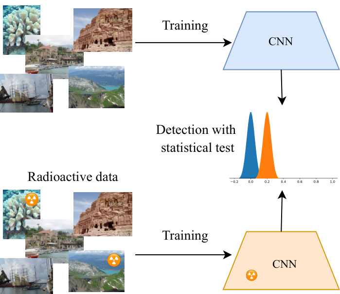
Figure 1. Illustration of our approach: we want to determine through a statistical test $\overset{\cdot}{p}$ -value) whether a network has seen a marked dataset or not. The distribution (shown on the histograms) of a statistic on the network weights is clearly separated between the vanilla and radioactive CNNs. Our method works in the cases of both white-box and black-box access to the network.
图 1: 方法示意图:我们希望通过统计检验($\overset{\cdot}{p}$值)判断网络是否接触过标记数据集。权重统计量的分布(直方图所示)在普通CNN和放射性CNN之间存在明显差异。该方法适用于白盒和黑盒网络访问场景。
solve specific tasks (e.g. classification, segmentation), but as a side-effect reproduce the bias in the datasets (Torralba et al., 2011). Such a bias is a weak signal that a particular dataset has been used to solve a task. Our objective in this paper is to enable the trace ability for datasets. By introducing a specific mark in a dataset, we want to provide a strong signal that a dataset has been used to train a model. We thus slightly change the dataset, effectively substituting the data for similar-looking marked data (isotopes).
解决特定任务(如分类、分割)的同时,会附带复现数据集中的偏差(Torralba et al., 2011)。这种偏差是特定数据集被用于解决任务的微弱信号。本文的目标是实现数据集的可追溯性。通过在数据集中引入特定标记,我们希望为"数据集被用于训练模型"这一事实提供强信号。因此我们对数据集进行微调,用视觉相似的标记数据(同位素)有效替换原始数据。
Let us assume that this data, as well as other collected data, is used to train a convolutional neural network (convnet). After training, the model is inspected to assess the use of radioactive data. The convnet is accessed either (1) explicitly when the model and corresponding weights are available (white-box setting), or (2) implicitly if only the decision scores are accessible (black-box setting). From that information, we answer the question of whether any radioactive data has been used to train the model, or if only vanilla data was used. We want to provide a statistical guarantee with the answer, in the form of a $p$ -value.
假设这些数据以及其他收集的数据被用于训练一个卷积神经网络 (convnet)。训练完成后,检查模型以评估放射性数据的使用情况。访问该卷积神经网络的方式有两种:(1) 显式访问(当模型及对应权重可用时,即白盒场景),或 (2) 隐式访问(仅能获取决策分数时,即黑盒场景)。基于这些信息,我们回答该模型是否使用了放射性数据进行训练,还是仅使用了普通数据。我们希望以 $p$ 值的形式为答案提供统计保证。
Passive techniques such as those employed to measure dataset bias (Torralba et al., 2011) or to do membership inference (S a blay roll es et al., 2019; Shokri et al., 2017) cannot provide sufficient empirical or statistical guarantees. More importantly, their measurement is relatively weak and therefore cannot be considered as an evidence: they are likely to confuse datasets having the same underlying statistics. In contrast, we target a $p$ -value much below $0.1%$ , meaning there is a very low probability that the results we observe are obtained by chance.
用于测量数据集偏差 (Torralba et al., 2011) 或进行成员推理 (S a blay roll es et al., 2019; Shokri et al., 2017) 的被动技术无法提供足够的实证或统计保证。更重要的是,它们的测量相对较弱,因此不能作为证据:它们可能会混淆具有相同基础统计特征的数据集。相比之下,我们的目标是 $p$ 值远低于 $0.1%$,这意味着我们观察到的结果纯属偶然的概率极低。
Therefore, we focus on active techniques, where we apply visually imperceptible changes to the images. We consider the following three criteria: (1) The change should be tiny, as measured by an image quality metric like PSNR (Peak Signal to Noise Ratio); (2) The technique should be reasonably neutral with respect to the end-task, i.e., the accuracy of the model trained with the marked dataset should not be significantly modified; (3) The method should not be detectable by a visual analysis of failure cases and should be immune to a re-annotation of the dataset. This disqualifies techniques that employ incorrect labels as a mark, which are easy to detect by a simple analysis of the failure cases. Similarly the “backdoor” techniques are easy to identify and circumvent with outlier detection (Tran et al., 2018).
因此,我们专注于主动技术,即对图像施加视觉上难以察觉的改动。我们考虑以下三个标准:(1) 改动应足够微小,可通过PSNR (峰值信噪比) 等图像质量指标衡量;(2) 该技术对终端任务应保持相对中立,即使用标记数据集训练的模型准确率不应受到显著影响;(3) 该方法不应通过对失败案例的视觉分析被检测到,且能抵御数据集的重新标注。这排除了使用错误标签作为标记的技术——通过简单分析失败案例即可轻易识别此类标记。同样地,"后门"技术也容易通过异常值检测被识别和规避 (Tran et al., 2018)。
At this point, one may draw the analogy between this problem and watermarking (Cox et al., 2002), whose goal is to imprint a mark into an image such that it can be reidentified with high probability. We point out that traditional image-based watermarking is ineffective in our context: the learning procedure ignores the watermarks if they are not useful to guide the classification decision (Tishby et al., 2000). Therefore regular watermarking leaves no exploitable trace after training. We need to force the network to keep the mark through the learning process, whatever the learning procedure or architecture.
此时,人们可能会将这一问题与水印技术 (Cox et al., 2002) 进行类比,后者的目标是在图像中嵌入标记,使其能够以高概率被重新识别。我们指出,传统的基于图像的水印技术在此场景下是无效的:如果水印对分类决策没有指导作用,学习过程会忽略这些水印 (Tishby et al., 2000)。因此常规水印在训练后不会留下可利用的痕迹。我们需要迫使网络在整个学习过程中保留标记,无论采用何种学习流程或架构。
To that goal, we propose radioactive data. As illustrated in Figure 1 and similarly to radioactive markers in medical applications, we introduce marks (data isotopes) that remain through the learning process and that are detectable with high confidence in a neural network. Our idea is to craft a class-specific additive mark in the latent space before the classification layer. This mark is propagated back to the pixels with a marking (pretrained) network.
为了实现这一目标,我们提出了放射性数据 (radioactive data) 的概念。如图 1 所示,类似于医学应用中的放射性标记物,我们引入了在学习过程中持续存在且能在神经网络中以高置信度检测到的标记(数据同位素)。我们的核心思想是在分类层之前的潜在空间中构建一个类别特定的加性标记,并通过一个标记(预训练)网络将该标记反向传播至像素空间。
This behaviour is confirmed by an analysis of the latent space before classification. It shows that the network devotes a small part of its capacity to keep track of our “radioactive tracers”.
这种行为通过对分类前的潜在空间分析得到了证实。分析表明,网络仅用一小部分容量来追踪我们的"放射性示踪剂"。
Our experiments on Imagenet confirm that our radioactive marking technique is effective: with almost invisible changes to the images $(\mathrm{PSNR}=42~\mathrm{dB})$ ), and when marking only a fraction of the images $\zeta_{q}=1%$ ), we are able to detect the use of our radioactive images with very strong confidence. Note that our radioactive marks, while visually imperceptible, might be detected by a statistical analysis of the latent space of the network. Our aim in this paper is to provide a proof of concept that marking data is possible with statistical guarantees, and the analysis of defense mechanisms lies outside the scope of this paper. The deep learning community has developed a variety of defense mechanisms against “adversarial attacks”: these techniques prevent test-time tampering, but are not designed to prevent training-time attacks on neural networks.
我们在ImageNet上的实验证实,放射性标记技术效果显著:在图像几乎无视觉变化 (PSNR=42 dB) 且仅标记少量图像 (ζq=1%) 的情况下,仍能以极高置信度检测出放射性图像的使用。需要注意的是,这些放射性标记虽无法被肉眼察觉,但可能通过对网络隐空间的统计分析被检测到。本文旨在提供具有统计保证的数据标记概念验证,防御机制分析不在研究范围内。深度学习社区已开发出多种对抗"对抗攻击 (adversarial attacks)"的防御技术:这些方法可防止测试阶段的篡改,但并非针对训练阶段神经网络攻击的防护设计。
Our conclusions are supported in various settings: we consider both the black-box and white-box settings; we change the tested architecture such that it differs from the one employed to insert the mark. We also depart from the common restrictions of many data-poisoning works (Shafahi et al., 2018; Biggio et al., 2012), where only the logistic layer is retrained, and which consider small datasets (CIFAR) and/or limited data augmentation. We verify that the radioactive mark holds when the network is trained from scratch on a radioactive Imagenet dataset with standard random data augmentations. As an example, for a ResNet-18 trained from scratch, we achieve a $p$ -value of $10^{-4}$ when only $1%$ of the training data is radioactive. The accuracy of the network is not noticeably changed $(\pm0.1%)$ .
我们的结论在多种设置下均得到验证:我们同时考虑了黑盒与白盒场景;调整了测试架构使其不同于用于植入标记的架构。我们还突破了多数数据投毒研究的常见限制(Shafahi等人,2018;Biggio等人,2012)——这些研究仅重新训练逻辑层,且仅针对小规模数据集(CIFAR)和/或有限的数据增强。实验证明,当网络在采用标准随机数据增强的放射性Imagenet数据集上从头训练时,放射性标记依然有效。例如,对于从头训练的ResNet-18,当仅1%的训练数据具有放射性时,我们获得了$p$值为$10^{-4}$的显著结果,且网络准确率未出现明显波动$(\pm0.1%)$。
The paper is organized as follows. Section 2 reviews the related literature. We discuss related works in watermarking, and explain how the problem that we tackle is related to and differs from data poisoning. In Section 3, after introducing a few mathematical notions, we describe how we add markers, and discuss the detection methods in both the white-box and black-box settings. Section 4 provides an analysis of the latent space learned with our procedure and compares it to the original one. We present qualitative and quantitative results in different settings in the experimental section 5. We conclude the paper in Section 6.
本文结构如下。第2节回顾相关文献,讨论水印技术的研究现状,并说明我们所解决的问题与数据投毒(data poisoning)的关联及区别。第3节在介绍数学概念后,阐述标记添加方法,并分析白盒(white-box)与黑盒(black-box)场景下的检测方案。第4节通过潜空间分析对比原始模型与改进模型的差异。第5节实验部分展示多场景下的定性与定量结果。第6节总结全文。
2. Related work
2. 相关工作
Watermarking is a way of tracking media content by adding a mark to it. In its simplest form, a watermark is an addition in the pixel space of an image, that is not visually perceptible. Zero-bit watermarking techniques (Cayre et al., 2005) modify the pixels of an image so that its Fourier transform lies in the cone generated by an arbitrary random direction, the “carrier”. When the same image or a slightly perturbed version of it are encountered, the presence of the watermark is assessed by verifying whether the Fourier representation lies in the cone generated by the carrier. Zero-bit watermarking detects whether an image is marked or not, but in general watermarking also considers the case where the marks carry a number of bits of information (Cox et al., 2002).
水印是一种通过添加标记来追踪媒体内容的方法。最简单的形式是在图像的像素空间中添加一个视觉上不可察觉的标记。零比特水印技术 (Cayre et al., 2005) 通过修改图像的像素,使其傅里叶变换位于由任意随机方向(即“载体”)生成的锥形区域内。当遇到相同图像或其轻微扰动版本时,通过验证傅里叶表示是否位于载体生成的锥形区域内来判断水印的存在。零比特水印仅检测图像是否被标记,而广义水印技术还考虑标记携带多位信息的情况 (Cox et al., 2002)。
Traditional watermarking is notoriously not robust to geometrical attacks (Vukotic et al., 2018). In contrast, the latent space associated with deep networks is almost invariant to such transformations, due to the train-time data augmentations. This observation has motivated several authors to employ convnets to watermark images (Vukotic et al., 2018; Zhu et al., 2018) by inserting marks in this latent space. HiDDeN (Zhu et al., 2018) is an example of these approaches, applied either for s tegan o graphic or watermarking purposes.
传统水印技术对几何攻击的脆弱性众所周知 (Vukotic et al., 2018) 。与之相反,由于训练时的数据增强操作,深度网络关联的潜在空间对此类变换几乎具有不变性。这一发现促使多位研究者采用卷积网络在潜在空间中嵌入标记来实现图像水印 (Vukotic et al., 2018; Zhu et al., 2018) 。HiDDeN (Zhu et al., 2018) 就是这类方法的代表,既可应用于隐写术也可用于数字水印。
Adversarial examples. Neural networks have been shown to be vulnerable to so-called adversarial examples (Carlini & Wagner, 2017; Goodfellow et al., 2015; Szegedy et al., 2014): given a correctly-classified image $x$ and a trained network, it is possible to craft a perturbed version $\tilde{x}$ that is visually indistinguishable from $x$ , such that the network mis classifies $\tilde{x}$ .
对抗样本 (adversarial examples)。研究表明神经网络易受所谓对抗样本的攻击 [20][21][22]:给定一个正确分类的图像$x$和一个训练好的网络,可以构造出视觉上与$x$无法区分的扰动版本$\tilde{x}$,使得网络对$\tilde{x}$产生误分类。
Privacy and membership inference. Differential privacy (Dwork et al., 2006) protects the privacy of training data by bounding the impact that an element of the training set has on a trained model. The privacy budget $\epsilon>0$ limits the impact that the substitution of one training example can have on the log-likelihood of the estimated parameter vector. It has become the standard for privacy in the industry and the privacy budget $\epsilon$ trades off between learning statistical facts and hiding the presence of individual records in the training set. Recent work (Abadi et al., 2016; Papernot et al., 2018) has shown that it is possible to learn deep models with differential privacy on small datasets (MNIST, SVHN) with a budget as small as $\epsilon=1$ . Individual privacy degrades gracefully to group privacy: when testing for the joint presence of a group of $k$ samples in the training set of a model, an $\epsilon$ -private algorithm provides guarantees of $k\epsilon$ .
隐私与成员推理。差分隐私 (Differential Privacy) (Dwork et al., 2006) 通过限制训练集中单个元素对训练模型的影响来保护训练数据的隐私。隐私预算 $\epsilon>0$ 限定了替换一个训练样本对估计参数向量对数似然的影响程度,现已成为工业界的隐私保护标准。该预算 $\epsilon$ 需要在学习统计事实与隐藏训练集中个体记录存在性之间进行权衡。近期研究 (Abadi et al., 2016; Papernot et al., 2018) 表明,在MNIST、SVHN等小数据集上,使用低至 $\epsilon=1$ 的预算即可训练具备差分隐私的深度学习模型。个体隐私可平滑退化为群体隐私:当检测模型训练集中 $k$ 个样本的联合存在性时,$\epsilon$-隐私算法可提供 $k\epsilon$ 的隐私保障。
Membership inference (Shokri et al., 2017; Carlini et al., 2018; S a blay roll es et al., 2019) is the reciprocal operation of differential ly private learning. It predicts from a trained model and a sample, whether the sample was part of the model’s training set. These classification approaches do not provide any guarantee: if a membership inference model predicts that an image belongs to the training set, it does not give a level of statistical significance. Furthermore, these techniques require training multiple models to simulate datasets with and without an image, which is computationally intensive.
成员推断 (Shokri et al., 2017; Carlini et al., 2018; Sablayrolles et al., 2019) 是差分隐私学习的逆向操作。该方法通过训练好的模型和样本预测该样本是否属于模型的训练集。这些分类方法不提供任何保证:若成员推断模型预测某图像属于训练集,其结论不具备统计显著性。此外,这些技术需要训练多个模型来模拟包含/不包含特定图像的数据集,计算成本高昂。
Data poisoning (Biggio et al., 2012; Steinhardt et al., 2017; Shafahi et al., 2018) studies how modifying training data points affects a model’s behavior at inference time. Backdoor attacks (Chen et al., 2017; Gu et al., 2017) are a recent trend in machine learning attacks. They choose a class $c$ , and add unrelated samples from other classes to this class $c$ , along with an overlayed “trigger” pattern; at test time, any sample having the same trigger will be classified in this class $c$ . Backdoor techniques bear similarity with our radioactive tracers, in particular their trigger is close to our carrier. However, our method differs in two main aspects. First we do “clean-label” attacks, i.e., we perturb training points without changing their labels. Second, we provide statistical guarantees in the form of a $p$ -value.
数据投毒 (Biggio et al., 2012; Steinhardt et al., 2017; Shafahi et al., 2018) 研究如何通过修改训练数据点来影响模型在推理时的行为。后门攻击 (Chen et al., 2017; Gu et al., 2017) 是机器学习攻击领域的新趋势。它们选择一个类别 $c$,并将其他类别的无关样本添加至该类别 $c$,同时叠加一个"触发器"图案;在测试阶段,任何带有相同触发器的样本都会被归类到该类别 $c$。后门技术与我们的放射性示踪剂有相似之处,尤其是其触发器与我们的载体 (carrier) 相近。但我们的方法在两个方面存在显著差异:首先我们实施的是"干净标签"攻击,即在保持样本标签不变的情况下扰动训练数据;其次我们以 $p$ 值的形式提供统计保证。
Watermarking deep learning models. A few works (Adi et al., 2018; Yeom et al., 2018) focus on watermarking deep learning models: these works modify the parameters of a neural network so that any downstream use of the network can be verified. Our assumption is different: in our case, we control the training data, but the training process is not controlled.
深度学习模型水印技术。部分研究 (Adi et al., 2018; Yeom et al., 2018) 专注于深度学习模型的水印:这些工作通过修改神经网络参数,使得该网络的任何下游使用都能被验证。我们的假设有所不同:在本研究中,我们控制训练数据,但不控制训练过程。
3. Our method
3. 我们的方法
In this section, we describe our method for marking data. It consists of three stages: the marking stage where the radioactive mark is added to the vanilla training images, without changing their labels. The training stage uses vanilla and/or marked images to train a multi-class classifier using regular learning algorithms. Finally, in the detection stage, we examine the model to determine whether marked data was used or not.
在本节中,我们将介绍数据标记方法。该方法包含三个阶段:标记阶段将放射性标记添加到原始训练图像中而不改变其标签;训练阶段使用原始图像和/或标记图像,通过常规学习算法训练多分类器;最后在检测阶段,通过检查模型来判断是否使用了标记数据。
We denote by $x$ an image, i.e. a 3 dimensional tensor with dimensions height, width and color channel. We consider a classifier with $C$ classes composed of a feature extraction function $\phi:x\mapsto\phi(x)\in\mathbb{R}^{d}$ (a convolutional neu- ral network) followed by a linear classifier with weights $(w_{i})_{i=1\dots C}\in\mathbb{R}^{d}$ . It classifies a given image $x$ as
我们用 $x$ 表示一张图像,即一个三维张量,其维度分别为高度、宽度和颜色通道。我们考虑一个具有 $C$ 个类别的分类器,它由特征提取函数 $\phi:x\mapsto\phi(x)\in\mathbb{R}^{d}$ (一个卷积神经网络) 和一个线性分类器组成,后者的权重为 $(w_{i})_{i=1\dots C}\in\mathbb{R}^{d}$。该分类器将给定图像 $x$ 分类为
$$
\operatorname*{argmax}_ {i=1\ldots C}w_{i}^{\top}\phi(x).
$$
$$
\operatorname*{argmax}_ {i=1\ldots C}w_{i}^{\top}\phi(x).
$$
3.1. Statistical preliminaries
3.1. 统计基础
Cosine similarity with a random unitary vector $u$ . Given a fixed vector $v$ and a random vector $u$ distributed uniformly over the unit sphere in dimension $d$ $(|u|_ {2}=1)$ ), we are interested in the distribution of their cosine similarity $c(u,v):=:u^{T}v/(|u|_ {2}|v|_{2})$ . A classic result from statistics (Iscen et al., 2017) shows that this cosine similarity follows an incomplete beta distribution with parameters $\begin{array}{r}{a=\frac{1}{2}}\end{array}$ and $\textstyle b={\frac{d-1}{2}}$ :
与随机单位向量 $u$ 的余弦相似度。给定固定向量 $v$ 和均匀分布在 $d$ 维单位球面上的随机向量 $u$ $(|u|_ {2}=1)$ ,我们关注其余弦相似度 $c(u,v):=:u^{T}v/(|u|_ {2}|v|_{2})$ 的分布。统计学经典结果表明 [20] ,该余弦相似度服从参数为 $\begin{array}{r}{a=\frac{1}{2}}\end{array}$ 和 $\textstyle b={\frac{d-1}{2}}$ 的不完全贝塔分布:
$$
\begin{array}{l}{\displaystyle\mathbb{P}(c(u,v)\geq\tau)=I_{\tau^{2}}\left(\frac{1}{2},\frac{d-1}{2}\right)}\ {\displaystyle=\frac{B_{\tau^{2}}\left(\frac{1}{2},\frac{d-1}{2}\right)}{B\left(\frac{1}{2},\frac{d-1}{2}\right)}}\ {\displaystyle=\frac{1}{B\left(\frac{1}{2},\frac{d-1}{2}\right)}\int_{0}^{\tau^{2}}\frac{\left(\sqrt{1-t}\right)^{d-3}}{\sqrt{t}}d t}\end{array}
$$
$$
\begin{array}{l}{\displaystyle\mathbb{P}(c(u,v)\geq\tau)=I_{\tau^{2}}\left(\frac{1}{2},\frac{d-1}{2}\right)}\ {\displaystyle=\frac{B_{\tau^{2}}\left(\frac{1}{2},\frac{d-1}{2}\right)}{B\left(\frac{1}{2},\frac{d-1}{2}\right)}}\ {\displaystyle=\frac{1}{B\left(\frac{1}{2},\frac{d-1}{2}\right)}\int_{0}^{\tau^{2}}\frac{\left(\sqrt{1-t}\right)^{d-3}}{\sqrt{t}}d t}\end{array}
$$
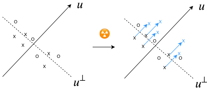
Figure 2. Illustration of our method in high dimension. In high dimension, the linear classifier that separates the class is almost orthogonal to $u$ with high probability. Our method shifts points belonging to a class in the direction $u$ , therefore aligning the linear classifier with the direction $u$ .
图 2: 高维空间中本方法的示意图。在高维情况下,区分类别的线性分类器几乎必然与向量 $u$ 正交。我们的方法将属于某类别的点沿 $u$ 方向平移,从而使线性分类器与 $u$ 方向对齐。
with
与
$$
B_{x}\left(\frac{1}{2},\frac{d-1}{2}\right)=\int_{0}^{x}\frac{\left(\sqrt{1-t}\right)^{d-3}}{\sqrt{t}}d t
$$
$$
B_{x}\left(\frac{1}{2},\frac{d-1}{2}\right)=\int_{0}^{x}\frac{\left(\sqrt{1-t}\right)^{d-3}}{\sqrt{t}}d t
$$
and
和
$$
B\left(\frac{1}{2},\frac{d-1}{2}\right)=B_{1}\left(\frac{1}{2},\frac{d-1}{2}\right).
$$
$$
B\left(\frac{1}{2},\frac{d-1}{2}\right)=B_{1}\left(\frac{1}{2},\frac{d-1}{2}\right).
$$
In particular, it has expectation 0 and variance $1/d$ .
特别地,其期望为0且方差为$1/d$。
Combination of $p$ -values. Fisher’s method (Fisher, 1925) enables to combine $p$ -values of multiple tests. We consider statistical tests $T_{1},\ldots,T_{k}$ , independent under the null hypothesis $\mathcal{H}{0}$ . Under $\mathcal{H}{0}$ , the corresponding $p$ - values $p_{1},\ldots,p_{k}$ are distributed uniformly in [0, 1]. Hence $-\log(p_{i})$ follows an exponential distribution, which corresponds to a $\chi^{2}$ distribution with two degrees of freedom. The quantity $\begin{array}{r}{Z=-2\sum_{i=1}^{k}\log(p_{i})}\end{array}$ thus follows a $\chi^{2}$ distribution with $2k$ deg rees of freedom. The combined $p$ - value of tests $T_{1},\ldots,T_{k}$ is thus the probability that the random variable $Z$ has a value higher than the threshold we observe.
$p$ 值的组合。Fisher方法 (Fisher, 1925) 能够合并多个检验的 $p$ 值。我们考虑统计检验 $T_{1},\ldots,T_{k}$,在原假设 $\mathcal{H}_ {0}$ 下相互独立。在 $\mathcal{H}_ {0}$ 下,对应的 $p$ 值 $p_{1},\ldots,p_{k}$ 服从 [0, 1] 上的均匀分布。因此 $-\log(p_{i})$ 服从指数分布,对应自由度为 2 的 $\chi^{2}$ 分布。量 $\begin{array}{r}{Z=-2\sum_{i=1}^{k}\log(p_{i})}\end{array}$ 则服从自由度为 $2k$ 的 $\chi^{2}$ 分布。因此检验 $T_{1},\ldots,T_{k}$ 的组合 $p$ 值是随机变量 $Z$ 取值高于观测阈值的概率。
3.2. Additive marks in feature space
3.2. 特征空间中的叠加标记
We first tackle a simple variant of our tracing problem. In the marking stage, we add a random isotropic unit vector $\alpha u\in\mathbb{R}^{d}$ with $|u|_{2}=1$ to the features of all training images of one class. This direction $u$ is our carrier.
我们首先解决追踪问题的一个简单变体。在标记阶段,我们向某一类别的所有训练图像特征中添加一个随机各向同性单位向量 $\alpha u\in\mathbb{R}^{d}$ (其中 $|u|_{2}=1$ )。这个方向 $u$ 就是我们的载体。
If radioactive data is used at training time, the linear classifier of the corresponding class $w$ is updated with weighted sums of $\phi(x)+\alpha u$ , where $\alpha$ is the strength of the mark. The linear classifier $w$ is thus likely to have a positive dot product with the direction $u$ , as shown in Figure 2.
如果在训练时使用了放射性数据,相应类别 $w$ 的线性分类器会通过 $\phi(x)+\alpha u$ 的加权和进行更新,其中 $\alpha$ 是标记强度。因此,线性分类器 $w$ 很可能与方向 $u$ 具有正点积,如图 2 所示。
At detection time, we examine the linear classifier $w$ to determine if $w$ was trained on radioactive or vanilla data. We test the statistical hypothesis $\mathcal{H}_ {1}$ : “ $w$ was trained using radioactive data” against the null hypothesis $\mathcal{H}_ {0}$ : “ $w$ was trained using vanilla data”. Under the null hypothesis $\mathcal{H}_ {0}$ , $u$ is a random vector independent of $w$ . Their cosine similarity $c(u,w)$ follows the beta-incomplete distribution with parameters $\begin{array}{r}{a=\frac{1}{2}}\end{array}$ and $\textstyle b={\frac{d-1}{2}}$ . Under hypothesis $\mathcal{H}_{1}$ , the classifier vector $w$ is more aligned with the direction $u$ so and $c(u,w)$ is likely to be higher.
在检测阶段,我们通过分析线性分类器 $w$ 来判断其训练数据是否包含放射性标记数据。我们检验统计假设 $\mathcal{H}_ {1}$ : "$w$ 使用放射性数据训练"与零假设 $\mathcal{H}_ {0}$ : "$w$ 使用原始数据训练"。在零假设 $\mathcal{H}_ {0}$ 下,$u$ 是与 $w$ 独立的随机向量,它们的余弦相似度 $c(u,w)$ 服从参数为 $\begin{array}{r}{a=\frac{1}{2}}\end{array}$ 和 $\textstyle b={\frac{d-1}{2}}$ 的Beta不完全分布。而在假设 $\mathcal{H}_{1}$ 下,分类器向量 $w$ 与方向 $u$ 更趋一致,因此 $c(u,w)$ 的值通常会更高。
Thus if we observe a high value of $c(u,w)$ , its corresponding $p$ -value (the probability of it happening under the null hypothesis $\mathcal{H}_{0}$ ) is low, and we can conclude with high significance that radioactive data has been used.
因此,如果我们观察到 $c(u,w)$ 值较高,其对应的 $p$ 值(在零假设 $\mathcal{H}_{0}$ 下发生的概率)较低,就能以高显著性判定数据含有放射性痕迹。
Multi-class. The extension to $C$ classes follows. In the marking stage we sample i.i.d. random directions $(u_{i})_ {i=1,..C}$ and add them to the features of images of class $i$ . At detection time, under the null hypothesis, the cosine similarities $c(u_{i},w_{i})$ are independent (since $u_{i}$ are independent) and we can thus combine the $p$ values for each class using Fisher’s combined probability test (Section 3.1) to obtain the $p$ value for the whole dataset.
多分类。扩展到 $C$ 类的情况如下:在标记阶段,我们独立同分布地采样随机方向 $(u_{i}){i=1,..C}$,并将其添加到类别 $i$ 的图像特征中。在检测阶段,根据零假设,余弦相似度 $c(u{i},w_{i})$ 是独立的(因为 $u_{i}$ 相互独立),因此我们可以使用费希尔组合概率检验(第3.1节)将每个类别的 $p$ 值组合起来,从而得到整个数据集的 $p$ 值。
3.3. Image-space perturbations
3.3. 图像空间扰动
We now assume that we have a fixed known feature extractor $\phi$ . At marking time, we wish to modify pixels of image $x$ such that the features $\phi(x)$ move in the direction $u$ . We can achieve this by back propagating gradients in the image space. This setup is very similar to adversarial examples (Goodfellow et al., 2015; Szegedy et al., 2014). More precisely, we optimize over the pixel space by running the following optimization program:
我们现在假设有一个固定的已知特征提取器$\phi$。在标记时,我们希望修改图像$x$的像素,使得特征$\phi(x)$沿着方向$u$移动。这可以通过在图像空间中反向传播梯度来实现。这种设置与对抗样本非常相似 [20][21]。更准确地说,我们通过运行以下优化程序在像素空间进行优化:
$$
\operatorname*{min}_ {\tilde{x},|\tilde{x}-x|_{\infty}\leq R}\mathcal{L}(\tilde{x})
$$
$$
\operatorname*{min}_ {\tilde{x},|\tilde{x}-x|_{\infty}\leq R}\mathcal{L}(\tilde{x})
$$
where the radius $R$ is a hard upper bound on the change of color levels of the image that we can accept. The loss is a combination of three terms:
其中半径 $R$ 是我们可接受的图像颜色级别变化的硬性上限。该损失由三项组合而成:
$$
\mathcal{L}(\tilde{{\boldsymbol{x}}})=-\left(\phi(\tilde{{\boldsymbol{x}}})-\phi({\boldsymbol{x}})\right)^{\top}{\boldsymbol{u}}+\lambda_{1}|\tilde{{\boldsymbol{x}}}-{\boldsymbol{x}}|_ {2}+\lambda_{2}|\phi(\tilde{{\boldsymbol{x}}})-\phi({\boldsymbol{x}})|_{2}.
$$
$$
\mathcal{L}(\tilde{{\boldsymbol{x}}})=-\left(\phi(\tilde{{\boldsymbol{x}}})-\phi({\boldsymbol{x}})\right)^{\top}{\boldsymbol{u}}+\lambda_{1}|\tilde{{\boldsymbol{x}}}-{\boldsymbol{x}}|_ {2}+\lambda_{2}|\phi(\tilde{{\boldsymbol{x}}})-\phi({\boldsymbol{x}})|_{2}.
$$
The first term encourages the features to align with $u$ , the two other terms penalize the $L_{2}$ distance in both pixel and feature space. In practice, we optimize this objective by running SGD with a constant learning rate in the pixel space, projecting back into the $L_{\infty}$ ball at each step and rounding to integral pixel values every $T=10$ iterations.
第一项鼓励特征与$u$对齐,另外两项惩罚像素空间和特征空间中的$L_{2}$距离。在实践中,我们通过在像素空间中运行具有恒定学习率的SGD (随机梯度下降) 来优化这一目标,每一步都投影回$L_{\infty}$球,并且每$T=10$次迭代就将像素值舍入为整数。
This procedure is a generalization of classical watermarking in the Fourier space. In that case the “feature extractor” is invertible via the inverse Fourier transform, so the marking does not need to be iterative.
该流程是对傅里叶空间经典水印技术的泛化。这种情况下,"特征提取器"可通过逆傅里叶变换实现可逆操作,因此水印标记无需迭代处理。
Data augmentation. The training stage most likely involves data augmentation, so we take it into account at marking time. Given an augmentation parameter $\theta$ , the input to the neural network is not the image $\tilde{x}$ but its transformed version $F(\theta,\tilde{x})$ . In practice, the data augmentations used are crop and/or resize transformations, so $\theta$ are the coordinates of the center and/or size of the cropped images. The augmentations are differentiable with respect to the pixel space, so we can back propagate through them. Thus, we emulate augmentations by minimizing:
数据增强。训练阶段很可能涉及数据增强,因此我们在标记时将其考虑在内。给定增强参数 $\theta$,神经网络的输入不是图像 $\tilde{x}$ 而是其变换版本 $F(\theta,\tilde{x})$。实践中使用的数据增强是裁剪和/或调整大小变换,因此 $\theta$ 是裁剪图像的中心坐标和/或尺寸。这些增强在像素空间上是可微的,因此我们可以通过它们进行反向传播。因此,我们通过最小化以下公式来模拟增强:
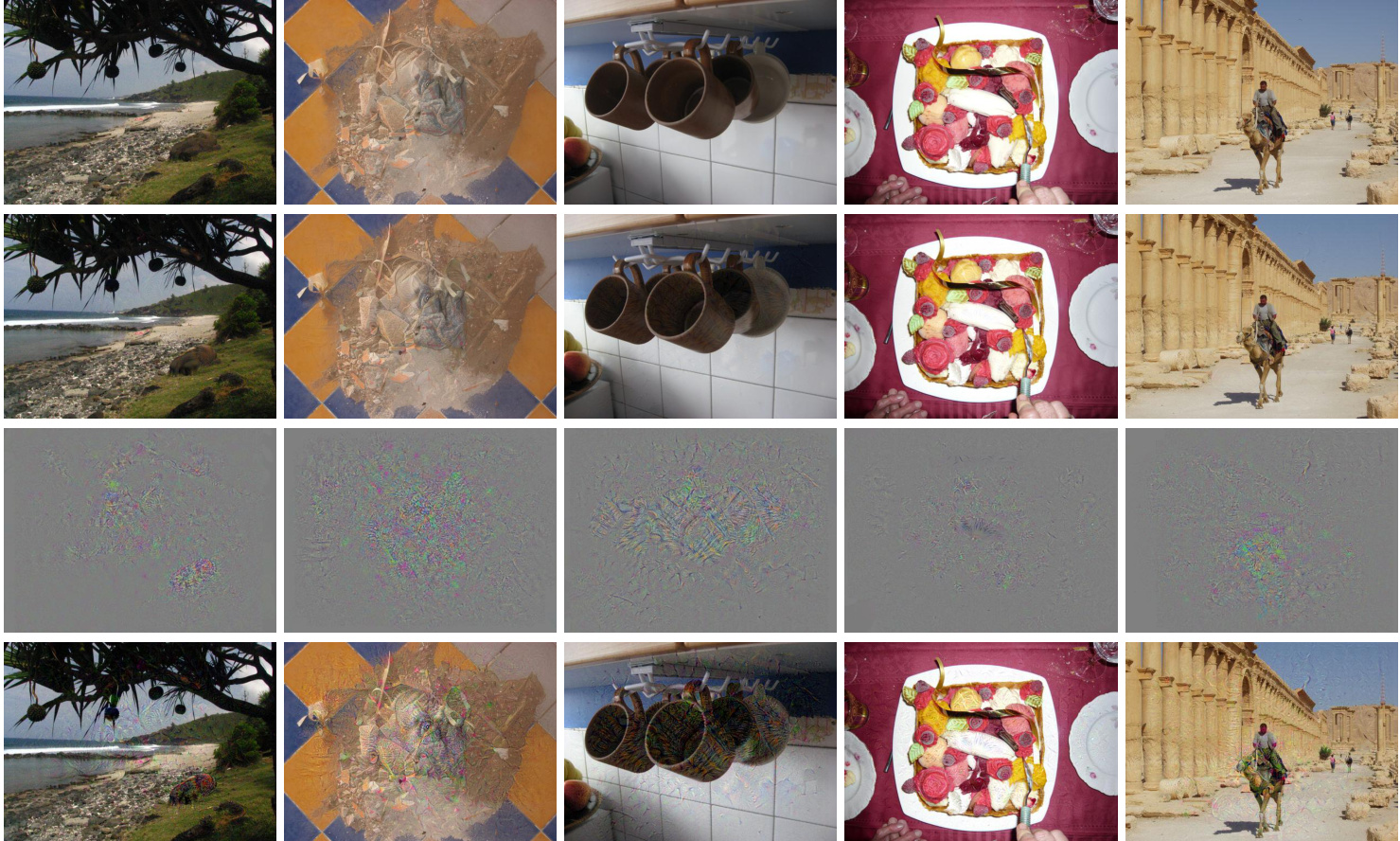
Figure 3. Radioactive images from Holidays (Jégou et al., 2008) with random crop and PSNR $=$ 42dB. First row: original image. Second row: image with a radioactive mark. Third row: visualisation of the mark amplified with a $\times5$ factor. Fourth row: We exaggerate the mark by a factor $\times5$ , which means a 14dB amplification of the additive noise, down to PSNR $\underline{{\underline{{\mathbf{\Pi}}}}}$ 28dB so that the modification become obvious w.r.t. the original image.
图 3: 来自Holidays (Jégou et al., 2008) 的放射性标记图像,采用随机裁剪且PSNR $=$ 42dB。第一行:原始图像。第二行:带放射性标记的图像。第三行:标记经 $\times5$ 因子放大后的可视化效果。第四行:我们将标记夸张放大 $\times5$ 倍,相当于对加性噪声进行14dB的放大,使PSNR降至 $\underline{{\underline{{\mathbf{\Pi}}}}}$ 28dB,从而使修改痕迹相对于原图变得明显可见。
To address this problem at detection time, we align the subspaces of the feature extractors. We find a linear mapping $\bar{\boldsymbol{M}}\in\mathbb{R}^{d\times d}$ such that $\phi_{0}(x)\approx M\phi_{t}(x)$ . The linear mapping is estimated by $L_{2}$ regression:
为解决检测时的问题,我们对特征提取器的子空间进行对齐。找到一个线性映射 $\bar{\boldsymbol{M}}\in\mathbb{R}^{d\times d}$ 使得 $\phi_{0}(x)\approx M\phi_{t}(x)$。该线性映射通过 $L_{2}$ 回归估计:
$$
\operatorname*{min}_ {M}\mathbb{E}_ {x}[|\phi_{0}(x)-M\phi_{t}(x)|_{2}^{2}].
$$
$$
\operatorname*{min}_ {M}\mathbb{E}_ {x}[|\phi_{0}(x)-M\phi_{t}(x)|_{2}^{2}].
$$
$$
\operatorname*{min}_ {\tilde{x},|\tilde{x}-x|_ {\infty}\leq R}\quad\mathbb{E}_{\theta}\left[\mathcal{L}(F(\tilde{x},\theta))\right].
$$
$$
\operatorname*{min}_ {\tilde{x},|\tilde{x}-x|_ {\infty}\leq R}\quad\mathbb{E}_{\theta}\left[\mathcal{L}(F(\tilde{x},\theta))\right].
$$
In practice, we use vanilla images of a held-out set (the validation set) to do the estimation.
在实践中,我们使用保留集(验证集)的原始图像进行估计。
Figure 3 shows examples of radioactive images and their vanilla version. We can see that the radioactive mark is not visible to the naked eye, except when we amplify it for visualization purposes (last column).
图 3: 展示了放射性图像及其原始版本的示例。可以看出,除非为了可视化目的进行放大(最后一列),否则放射性标记肉眼不可见。
3.4. White-box test with subspace alignment
3.4. 基于子空间对齐的白盒测试
We now tackle the more difficult case where the training stage includes the training of the feature extractor. In the marking stage we use feature extractor $\phi_{0}$ to generate radioactive data. At training time, a new feature extractor $\phi_{t}$ is trained together with the classification matrix $W=[w_{1},..,w_{C}]^{T}\in\mathbb{R}^{C\times d}$ . Since $\phi_{t}$ is trained from scratch, there is no reason that the output spaces of $\phi_{0}$ and $\phi_{t}$ would correspond to each other. In particular, neural networks are invariant to permutation and rescaling.
我们现在处理更复杂的情况,即训练阶段包含特征提取器的训练。在标记阶段,我们使用特征提取器 $\phi_{0}$ 生成放射性数据。训练时,新的特征提取器 $\phi_{t}$ 与分类矩阵 $W=[w_{1},..,w_{C}]^{T}\in\mathbb{R}^{C\times d}$ 一起训练。由于 $\phi_{t}$ 是从头开始训练的,$\phi_{0}$ 和 $\phi_{t}$ 的输出空间没有必然的对应关系。特别是,神经网络对排列和缩放具有不变性。
The classifier we manipulate at detection time is thus $W\phi_{t}(x)\approx W M\phi_{0}(x)$ . The lines of $W M$ form classification vectors aligned with the output space of $\phi_{0}$ , and we can compare these vectors to $u_{i}$ in cosine similarity. Under the null hypothesis, $u_{i}$ are random vectors independent of $\phi_{0},\phi_{t}$ , $W$ and $M$ and thus the cosine similarity is still given by the beta incomplete function, and we can apply the techniques of subsection 3.2.
我们在检测时操作的分类器因此为 $W\phi_{t}(x)\approx W M\phi_{0}(x)$ 。$W M$ 的各行构成了与 $\phi_{0}$ 输出空间对齐的分类向量,我们可以通过余弦相似度将这些向量与 $u_{i}$ 进行比较。在原假设下,$u_{i}$ 是与 $\phi_{0},\phi_{t}$、$W$ 和 $M$ 无关的随机向量,因此余弦相似度仍由不完全贝塔函数给出,我们可以应用第3.2小节的技术。
3.5. Black-box test
3.5. 黑盒测试
In the case where we do not have access to the weights of the neural network, we can still assess whether the model has seen contaminated images by analyzing its loss $\ell(W\phi_{t}(x),y)$ . If the loss of the model is lower on marked images than on vanilla images, it indicates that the model was trained on radioactive images. If we have unlimited access to a black-box model, it is possible to train a student model that mimicks the outputs of the black-box model. In that case, we can map back the problem to an analysis of the white-box student model.
在我们无法获取神经网络权重的情况下,仍可通过分析其损失函数 $\ell(W\phi_{t}(x),y)$ 来评估模型是否接触过污染图像。若模型在标记图像上的损失低于原始图像,则表明该模型曾使用放射性图像进行训练。若对黑盒模型具有无限访问权限,则可训练一个模仿黑盒模型输出的学生模型,此时该问题可转化为对白盒学生模型的分析。

Figure 4. Decomposition of learned class if i ers into three parts: the “semantic direction” (y-axis), the carrier direction $\mathbf{\rho}_{\mathrm{X}}$ -axis) and noise (represented by $1-|x|^{2}-|y|^{2}$ , i.e. the distance between a point and the unit circle). The semantic and carrier direction are 1-D subspace, while the noise corresponds to the complementary (high-dim) subspace. Colors represent the percentage of radioactive data in the training set, from $q=1%$ (dark blue) to $q=50%$ (yellow). Even when $q=50%$ of the data is radioactive, the learned classifier is still aligned with its semantic direction with a cosine similarity of 0.6. Each dot represents the classifier for a given class. Note that the semantic and the carrier directions are not exactly orthogonal but their cosine similarity is very small (in the order of 0.04).
图 4: 学习到的分类器分解为三部分:"语义方向"(y轴)、载体方向 $\mathbf{\rho}_{\mathrm{X}}$ (x轴)和噪声(由 $1-|x|^{2}-|y|^{2}$ 表示,即点到单位圆的距离)。语义方向和载体方向是1维子空间,而噪声对应于互补的(高维)子空间。颜色表示训练集中放射性数据的百分比,从 $q=1%$ (深蓝)到 $q=50%$ (黄色)。即使当 $q=50%$ 的数据具有放射性时,学习到的分类器仍与其语义方向对齐,余弦相似度为0.6。每个点代表特定类别的分类器。注意语义方向和载体方向并非完全正交,但它们的余弦相似度非常小(约为0.04量级)。
4. Analysis of the latent feature space
4. 潜在特征空间分析
In this section, we analyze how the classifier learned on a radioactive dataset is related to (1) a classifier learned on unmarked images ; and (2) the direction of the carrier. For the sake of analysis, we take the simplest case where the mark is added in the latent feature space just before the classification layer, and we assume that only the logistic regression has been re-trained.
在本节中,我们分析了在放射性数据集上训练的分类器与以下两者的关系:(1) 在未标记图像上训练的分类器;(2) 载波方向。为了便于分析,我们采用最简单的情况:标记仅在分类层之前的潜在特征空间中添加,并假设仅重新训练了逻辑回归部分。
For a given class, we analyze how the classifier learned with a mark is explained by
对于给定的类别,我们分析带有标记的分类器是如何被解释的

Figure 5. Analysis of how classification directions re-learned with a logistic regression on marked images can be decomposed between (1) the original subspace; (2) the mark subspace; (3) the noise space. Logistic regression with: $q=2%$ (Left) or $q=20%$ $(R i g h t)$ of the images marked.
图 5: 分析在标记图像上通过逻辑回归重新学习的分类方向如何分解为 (1) 原始子空间; (2) 标记子空间; (3) 噪声空间。逻辑回归采用: $q=2%$ (左图) 或 $q=20%$ (右图) 的标记图像比例。
tion and the optimization procedure (SGD and random data augmentations).
训练过程和优化步骤 (SGD 和随机数据增强)。
The rationale of performing this decomposition is to quantify, with respect to the norm of the vector, what is the dominant subspace depending on the fraction of marked data.
执行这种分解的原理是为了量化向量范数中,主导子空间如何随标记数据比例而变化。
This decomposition is analyzed in Figure 4, where we make two important observations. First, the 2-dimensional subspace contains most of the projection of the new vector, which can be seen by the fact that the norm of the vector projected onto that subspace is close to 1 (which translates visually as to be close to the unit circle). Second and unsurprisingly, the contribution of the semantic vector is significant and still dominant compared to the mark, even when most of the dataset is marked. This property explains why our procedure has only a little impact on the accuracy.
该分解过程在图4中进行了分析,我们从中得出两个重要发现。首先,二维子空间包含了新向量的主要投影分量,这体现在投影到该子空间的向量范数接近1(视觉上表现为接近单位圆)。其次,即使大部分数据集被标记,语义向量的贡献依然显著且占主导地位,这一现象并不令人意外。该特性解释了为何我们的流程对准确率影响甚微。
Figure 5 shows the histograms of cosine similarities between the class if i ers and random directions, the mark direction and the semantic direction. We can see that the class if i ers are well aligned with the mark when $q=20%$ or $2%$ of the data is marked.
图 5: 展示了类别分类器与随机方向、标记方向以及语义方向之间余弦相似度的直方图。可以看出,当 $q=20%$ 或 $2%$ 的数据被标记时,类别分类器与标记方向高度对齐。
5. Experiments
5. 实验
5.1. Image classification setup
5.1. 图像分类设置
In order to provide a comparison on the widely-used vision benchmarks, we use Imagenet (Deng et al., 2009), a dataset of natural images with 1,281,167 images belonging to $1,000$ classes. We first consider the Resnet-18 and Resnet-50 models (He et al., 2016). We perform training using the standard set of data augmentations from Pytorch (Paszke et al., 2017). We train with SGD with a momentum of 0.9 and a weight decay of $10^{-4}$ for 90 epochs, using a batch size of 2048 across 8 GPUs. We use Pytorch (Paszke et al., 2017) and adopt its standard data augmentation settings (random crop resized to $224\times224$ ). We use the waterfall learning rate schedule: the learning starts at 0.8, (as recommended in (Goyal et al., 2017)) and is divided by 10 every 30 epochs. On a vanilla Imagenet, we obtain a top 1 accuracy of $69.6%$ and a top-5 accuracy of
为了在广泛使用的视觉基准测试上提供对比,我们采用了Imagenet (Deng et al., 2009) 数据集,该数据集包含1,281,167张自然图像,涵盖$1,000$个类别。我们首先选用Resnet-18和Resnet-50模型 (He et al., 2016),基于Pytorch (Paszke et al., 2017) 的标准数据增强集进行训练。训练使用带动量0.9的SGD优化器,权重衰减为$10^{-4}$,共进行90轮迭代,在8块GPU上采用2048的批量大小。我们使用Pytorch (Paszke et al., 2017) 并沿用其标准数据增强设置(随机裁剪调整至$224\times224$分辨率)。学习率采用瀑布式调度:初始值为0.8(遵循Goyal et al., 2017的建议),每30轮下降为原值的1/10。在原始Imagenet上,我们取得了$69.6%$的top-1准确率和
$89.1%$ with our Resnet18. We ran experiments by varying the random initialization and the order of elements seen during SGD, and found that the top 1 accuracy varies by $0.1%$ from one experiment to the other.
使用我们的Resnet18达到了89.1%的准确率。我们通过改变随机初始化和SGD过程中元素的顺序进行了实验,发现不同实验间的最高准确率差异为0.1%。
5.2. Experimental setup and metrics
5.2. 实验设置与评估指标
We modify Imagenet images by inserting our radioactive mark, and retrain models on this radioactive data using the learning algorithm described above. We then analyze these “contaminated” models for the presence of our mark. We report several measures of performance. On the images, we report the PSNR, i.e. the magnitude of the perturbation necessary to add the radioactive mark. On the model, we report the $p$ -value that measures how confident we are that radioactive data was used to train the model, as well as the accuracy of this model on vanilla (held-out) data. We conduct experiments where we only mark a fraction $q$ of the data, with $q\in{0.01,0.02,0.05,0.1,0.2}$ .
我们通过在Imagenet图像中插入放射性标记来修改图像,并使用上述学习算法在这些放射性数据上重新训练模型。随后分析这些"污染"模型是否存在我们的标记。我们报告了多项性能指标:在图像方面,报告了PSNR (即添加放射性标记所需的扰动幅度);在模型方面,报告了衡量模型训练数据是否含放射性数据的$p$值,以及该模型在原始(保留)数据上的准确率。实验设置了不同标记比例$q$ ($q\in{0.01,0.02,0.05,0.1,0.2}$) 进行验证。
As a sanity check, we ran our radioactive detector on pretrained models of the Pytorch zoo and found $p$ values of $15%$ for Resnet-18 and $51%$ for Resnet-50, which is reasonable: in the absence of radioactive data, these values should be uniformly distributed between 0 and 1.
作为验证,我们在Pytorch模型库的预训练模型上运行了放射性检测器,发现Resnet-18的$p$值为$15%$,Resnet-50的$p$值为$51%$。这一结果符合预期:在没有放射性数据的情况下,这些值应均匀分布在0到1之间。
5.3. Preliminary experiment: comparison to the backdoor technique
5.3. 初步实验:与后门技术的对比
We experimented with the backdoor technique of Chen et al. (Chen et al., 2017) in the context of our marking problem. In general, the backdoor technique adds unrelated images to a class, plus a “trigger” that is consistent across these added images. In their work, Chen et al. need to poison approximately $10%$ of the data in a class to activate their trigger. We adapted their technique to the “cleanlabel” setup on Imagenet: we blend a trigger (a Gaussian pattern) to images of a class. We observed that it is possible to detect this trigger at train time, albeit with a low image quality $(\mathrm{PSNR}<30\mathrm{dB})$ ) that is visually perceptible. In this case, the model is more confident on images that have the trigger than on vanilla images in about $90%$ of the cases. However, we also observed that any Gaussian noise activates the trigger: hence we have no guarantee that images with our particular mark were used.
我们针对标记问题测试了Chen等人 (Chen et al., 2017) 的后门技术。该技术通常会在某类别中添加无关图像,并给这些图像加上统一的"触发器"。Chen等人在研究中需要污染约$10%$的类别数据才能激活其触发器。我们将该技术适配到Imagenet的"干净标签"场景:通过向某类别图像混入高斯模式触发器。实验发现,虽然图像质量较低 $(\mathrm{PSNR}<30\mathrm{dB})$ 且肉眼可辨,但仍可能在训练时检测到该触发器。在此情况下,模型对含触发器图像的置信度在约$90%$的案例中高于原始图像。但我们也发现任何高斯噪声都能激活该触发器,因此无法确保特定标记图像被使用。
5.4. Results
5.4. 结果
Same architecture. We first analyze the results in Table 1 of a ResNet-18 model with fixed features trained on Imagenet. We can see that we are able to detect that our model was trained on radioactive data with a very high confidence for both center crop and random crop. The model overfits more on the center crop, hence it learns more the radioactive mark, which is why the $p$ -value is lower on center
相同架构。我们首先分析表1中在Imagenet上训练的固定特征ResNet-18模型结果。可以看到,无论是中心裁剪还是随机裁剪,我们都能以极高置信度检测出模型是在放射性数据上训练的。模型在中心裁剪上过拟合更严重,因此会更多地学习放射性标记,这就是中心裁剪的$p$值更低的原因。
Table 1. $p$ -value (statistical significance) for the detection of radioactive data usage when only a fraction of the training data is radioactive. Results for a logistic regression classifier trained on Imagenet with Resnet-18 features , with only a percentage of the data bearing the radioactive mark. Our method can identify with a very high confidence $(\log_{10}(p)<-38)$ that the classifier was trained on radioactive data, even when only $1%$ of the training data is radioactive. The radioactive data has an impact on the accuracy of the classifier: around $-1%$ (top-1).
| %radioactive 1 | 2 | 5 | 10 | |
| enter rop | log10 (p) <-150 acc -0.48 | <-150<-150<-150 -0.86 -1.07 -1.33 | ||
| uopun do | log1o (p) acc | -38.0-138.2<-150<-150 -0.24 | -0.31 -0.55 -0.99 | |
表 1: 当只有部分训练数据具有放射性标记时,检测放射性数据使用的$p$值(统计显著性)。基于Resnet-18特征在Imagenet上训练的逻辑回归分类器结果,其中仅有特定比例的数据带有放射性标记。我们的方法能以极高置信度$(\log_{10}(p)<-38)$识别分类器是在放射性数据上训练的,即使仅有$1%$的训练数据具有放射性。放射性数据对分类器准确率的影响约为$-1%$(top-1)。
| %放射性 | 1 | 2 | 5 | 10 |
|---|---|---|---|---|
| enter rop | log10(p)<-150 acc -0.48 | <-150<-150<-150 -0.86 -1.07 -1.33 | ||
| uopun do | log1o(p) acc | -38.0-138.2<-150<-150 -0.24 | -0.31 -0.55 -0.99 |
| %radioactive | 5 | 10 | |
| enter Crop log1o (p) | -0.66 -1.64 -4.60 -11.37 | ||
| dor log1o(p) | -4.85 -12.63 -48.8 | <-150 | |
| op acc | -0.1 -0.7 | -0.3 | -0.5 |
| %radioactive | 5 | 10 | |
|---|---|---|---|
| enter Crop log1o (p) | -0.66 -1.64 -4.60 -11.37 | ||
| dor log1o(p) | -4.85 -12.63 -48.8 | <-150 | |
| op acc | -0.1 -0.7 | -0.3 | -0.5 |
Table 2. $p$ -value (statistical significance) for radioactivity detection. Results for a Resnet-18 trained from scratch on Imagenet, with only a percentage of the data bearing the radioactive mark. We are able to identify models trained from scratch on only $q=1%$ of radioactive data. The presence of radioactive data has negligible impact on the accuracy of a learned model as long as the fraction of radioactive data is under $10%$ .
表 2: 放射性检测的 $p$ 值 (统计显著性) 。结果显示,在仅含 $q=1%$ 放射性标记数据的情况下,从头训练于Imagenet的Resnet-18模型仍可被识别。当放射性数据占比低于 $10%$ 时,其对模型准确率的影响可忽略不计。
crop images. Conversely on random crops, marking data has less impact on the accuracy of the model $(-0.24\$ as opposed to $-0.48$ for $q=1%$ marked data).
在随机裁剪的情况下,标记数据对模型准确率的影响较小($q=1%$标记数据时影响为$-0.24$,而非$-0.48$)。
Table 2 shows the results of retraining a Resnet-18 from scratch on radioactive data. The results confirm that our watermark can be detected when only $q=1%$ of the data is used at train time. This setup is more complicated for our marks because since the network is retrained from scratch, the directions that will be learned in the new feature space have no a priori reason to be aligned with the directions of the network we used. Table 2 shows two interesting results: first, the gap in accuracy is less important than when retraining only the logistic regression layer, in particular using $1%$ of radioactive data does not impact accuracy; second, data augmentation is actually helping the radioactive process. We hypothesize that the multiple crops make the network believe it sees more variety, but in reality all the feature representations of these crops are aligned with our carrier which makes the network learn the carrier direction.
表 2 展示了在放射性数据上从头开始重新训练 Resnet-18 的结果。这些结果证实,即使在训练时仅使用 $q=1%$ 的数据,我们的水印也能被检测到。这种设置对我们的标记来说更为复杂,因为由于网络是重新训练的,新特征空间中学习到的方向与我们使用的网络方向没有先验的对齐理由。表 2 显示了两项有趣的结果:首先,与仅重新训练逻辑回归层相比,准确率的差距较小,特别是使用 $1%$ 的放射性数据不会影响准确率;其次,数据增强实际上有助于放射性过程。我们假设多重裁剪让网络认为它看到了更多变化,但实际上这些裁剪的特征表示都与我们的载体对齐,这使得网络学习到了载体方向。

Figure 6. Black-box detection of the usage of radioactive data. The gap between the loss on radioactive and vanilla samples is around 0 when $q=20%$ of the data are contaminated.
图 6: 放射性数据使用的黑盒检测。当数据污染比例为 $q=20%$ 时,放射性样本与原始样本的损失差值接近0。
Black-box results. We report in Figure 6 the results of our black-box detection test. We measure the difference between the loss on vanilla samples and the loss on radioactive samples: when this gap is positive, it means that the model fares better on radioactive images, and thus that it has been trained on the radioactive data. We can see that the use of radioactive data can be detected when a fraction of $q=20%$ or more of the training set is radioactive. When a smaller portion of the data is radioactive, the model fares better on vanilla data than on radioactive data and thus it is difficult to tell.
黑盒测试结果。我们在图6中展示了黑盒检测测试的结果。我们测量了原始样本损失与放射性样本损失之间的差异:当该差值为正时,表明模型在放射性图像上表现更好,说明其训练数据包含放射性数据。可以看到,当训练集中放射性数据占比达到$q=20%$或更高时,放射性数据的使用可被检测到。若放射性数据占比较小,模型在原始数据上的表现优于放射性数据,此时难以判定。
Distillation. Given only black-box access to a model (assuming access to the full softmax), we experiment distillation of this model, and test the distilled model for radioac- tivity. In this setup, it is possible to detect the use of radioactive data on the distilled model, with a slightly lower performance compared to white-box access to the model. We give detailed results in Appendix A.
蒸馏。假设仅能通过黑盒访问模型(可获取完整的softmax输出),我们对该模型进行蒸馏实验,并测试蒸馏后模型的放射性。在此设置下,尽管性能略低于白盒访问模型,仍可检测出蒸馏模型使用了放射性数据。附录A提供了详细实验结果。
5.5. Ablation analysis
5.5. 消融分析
Architecture transfer. We ran experiments on different architectures with the same training procedure: Resnet-50, VGG-16 and Dense net 121. The results are shown in Table 3: the values and trend are similar to what we obtain with Resnet-18 (Table 2). This is non-trivial, as there is no reason that the feature space of a VGG-16 would behave in the same way as that of a Resnet-18: yet, after alignment, we are able to detect the presence of our radioactive mark with high statistical significance. Specifically, when $q=2%$ of the data is radioactive, we are able to detect it with a $p$ -value of $10^{-15}$ . This $p$ -value is even stronger than the one we obtain when retraining the same architecture as our marking architecture (Resnet-18). We hypothesize that larger model overfit more in general, and thus in this case will learn the mark more acutely.
架构迁移。我们在相同训练流程下对不同架构进行了实验:Resnet-50、VGG-16和DenseNet-121。结果如 表 3 所示:数值和趋势与Resnet-18( 表 2 )的结果相似。这一发现意义重大,因为VGG-16的特征空间本没有理由与Resnet-18表现相同:但在对齐后,我们仍能以高统计显著性检测到放射性标记的存在。具体而言,当 $q=2%$ 的数据具有放射性时,我们检测到的 $p$ 值达到 $10^{-15}$ 。该 $p$ 值甚至强于我们在使用与标记架构相同架构(Resnet-18)重新训练时获得的结果。我们假设更大模型通常更容易过拟合,因此在这种情况下会更敏锐地学习到标记特征。
Table 3. $p$ -value (statistical significance) for radioactivity detection. Results for different architectures trained from scratch on Imagenet. Even though radioactive data was crafted using a ResNet-18, models of other architectures also become radioactive when trained on this data.
| %radioactive | 1 | 5 | 10 20 |
| Resnet-50 -6.9 | -12.3-50.22-131.09 | <-150 | |
| <-150 | |||
| VGG-16-2.14 | -4.49 -13.01 | -33.28 -106.56 |
表 3: 放射性检测的 $p$ 值(统计显著性)。不同架构模型在Imagenet上从头训练的结果。尽管放射性数据是用ResNet-18生成的,但其他架构的模型在此数据上训练后也会具有放射性。
| %radioactive | 1 | 5 | 10 20 |
|---|---|---|---|
| Resnet-50 -6.9 | -12.3-50.22-131.09 | <-150 | |
| <-150 | |||
| VGG-16-2.14 | -4.49 -13.01 | -33.28 -106.56 |
Table 4. $p$ -value of radioactivity detection. A Resnet-18 is trained on Places205 from scratch, and a percentage of the dataset is radioactive. When $10%$ of the data or more is radioactive, we are able to detect radioactivity with a strong confidence $(p<10^{-3})$ ).
| %radioactive 10 |
| 20 50 100 log1o(p) -3.30 -8.14 -11.57 7<-150 |
表 4: 放射性检测的 $p$ 值。在Places205上从头训练Resnet-18模型,数据集中有一定比例的放射性数据。当 $10%$ 或更多数据具有放射性时,我们能够以高度置信度 $(p<10^{-3})$ 检测到放射性。
| %放射性 | 10 | 20 | 50 | 100 |
|---|---|---|---|---|
| log10(p) | -3.30 | -8.14 | -11.57 | <-150 |
Transfer to other datasets. We conducted experiments on a slightly different setup: we mark images from the dataset Places205, but use a network pretrained on Imagenet for the marking phase. These experiments show that even if the marking network is fit for a different distribution, the marking still works and we are able to detect it. Results are shown in Table 4. We can see that when a fraction q higher than $10%$ of the training data is marked, we can detect radioactivity with a strong statistical significance $(p<10^{-3})$ .
迁移到其他数据集。我们在稍有不同的设置下进行了实验:标记来自Places205数据集的图像,但在标记阶段使用在Imagenet上预训练的网络。这些实验表明,即使标记网络适用于不同的分布,标记仍然有效且可被检测到。结果如表4所示。可以看到,当训练数据中被标记部分比例q高于$10%$时,我们能够以极强的统计显著性$(p<10^{-3})$检测到放射性。
Correlation with class difficulty. Given that radioactive data adds a marker in the features that is correlated with the class label, we expect this mark to be learned by the network more when the class accuracy is low. To validate this hypothesis, we compute the Spearman correlation between the class accuracy for each class and the cosine between the classifier and the carrier: this correlation is negative, with a $p$ -value of $4\times10^{-5}$ . This confirms that the network relies more on the mark when learning with difficult classes.
与类别难度的相关性。鉴于放射性数据在特征中添加了与类别标签相关的标记,我们预期当类别准确率较低时,网络会更多地学习这一标记。为验证这一假设,我们计算了每个类别的准确率与分类器和载体之间余弦相似度的Spearman相关性:该相关性为负值($p$值为$4\times10^{-5}$),证实网络在学习困难类别时更依赖该标记。
5.6. Discussion
5.6. 讨论
The experiments validate that our radioactive marks do indeed imprint on the trained models. We also observe two beneficial effects: data augmentation improves the strength of the mark, and transferring the mask to a larger and more realistic architectures makes its detection more reliable. These two observations suggest that our radioactive method is appropriate for real use cases.
实验验证了我们的放射性标记确实会在训练后的模型中留下印记。我们还观察到两个有益效果:数据增强提高了标记的强度,将掩码迁移到更大更真实的架构中使其检测更加可靠。这两点观察表明,我们的放射性方法适用于实际应用场景。
Limitation in an adversarial scenario. We assume that at training time, there is no special procedure to take into account the radioactive data, but rather training is conducted as if it was vanilla data. In particular, a subspace analysis would likely reveal the marking direction. This adversarial scenario becomes akin to that considered in the watermarking literature, where strategies have been developed to reduce the detect ability of the carrier. Our current proposal is therefore restricted to the proof of concept that we can mark a model through training that is only resilient to blind attacks such as architectural or training changes. We hope that follow-up works will address a more challenging scenario under Kerckhoffs assumptions (Kerckhoffs, 1883).
对抗场景中的局限性。我们假设在训练时没有专门处理放射性数据的特殊流程,而是像处理普通数据一样进行训练。具体而言,子空间分析很可能会揭示标记方向。这种对抗场景类似于数字水印文献中讨论的情况,其中已开发出降低载体可检测性的策略。因此,我们当前的方案仅限于概念验证:通过训练对模型进行标记只能抵御架构或训练变更等盲攻击。我们希望后续研究能在Kerckhoffs假设 (Kerckhoffs, 1883) 下解决更具挑战性的场景。
6. Conclusion
6. 结论
The method proposed in this paper, radioactive data, is a way to verify if some data was used to train a model, with statistical guarantees.
本文提出的方法 radioactive data 是一种验证某些数据是否用于训练模型的方式,具有统计保证。
We have shown in this paper that such radioactive contamination is effective on large-scale computer vision tasks such as classification on Imagenet with modern architecture (Resnet-18 and Resnet-50), even when only a very small fraction $(1%)$ of the training data is radioactive. Although it is not the core topic of our paper, our method incidentally offers a way to watermark images in the classical sense (Cayre et al., 2005).
我们在本文中证明,这种放射性污染对大规模计算机视觉任务(如使用现代架构 Resnet-18 和 Resnet-50 在 Imagenet 上进行分类)是有效的,即使只有极少部分 $(1%)$ 的训练数据具有放射性。虽然这不是本文的核心主题,但我们的方法附带提供了一种经典意义上的图像水印方案 (Cayre et al., 2005)。
References
参考文献
| %radioactive | 1 | 2 | 5 | 10 | 20 |
| %radioactive | 1 | 2 | 5 | 10 | 20 |
|---|---|---|---|---|---|
Table 5. $p$ -value for the detection of radioactive data usage. A Resnet-18 is trained on Imagenet from scratch, and a percentage of the training data is radioactive. This marked network is distilled into another network, on which we test radioactivity. When $2%$ of the data or more is radioactive, we are able to detect the use of this data with a strong confidence $(p<10^{-3})$ ).
表 5: 放射性数据使用检测的 $p$ 值。在Imagenet上从头训练Resnet-18,其中部分训练数据具有放射性标记。该标记网络通过蒸馏迁移至另一网络,并在该网络上测试放射性。当 $2%$ 或更多数据具有放射性时,我们能够以极高置信度 $(p<10^{-3})$ 检测到该数据的使用。
A. Distillation
A. 蒸馏
Given a marked resnet-18 on which we only have blackbox access, we use distillation (Hinton et al., 2015) to train a second network. On this distilled network, we perform the radioactivity test. We show in Table 5 the results of this radioactivity test on distilled networks. We can see that when $2%$ or more of the original training data is radioactive, the radioactivity propagates through distillation with statistical significance $(p<10^{-3}\$ ).
给定一个只能进行黑盒访问的标记resnet-18,我们使用蒸馏 (Hinton et al., 2015) 训练第二个网络。在这个蒸馏网络上,我们执行放射性测试。表5展示了蒸馏网络上的放射性测试结果。可以看到,当原始训练数据中有2%或更多具有放射性时,放射性会通过蒸馏传播且具有统计显著性 $(p<10^{-3}\$)。