Fast reinforcement learning with generalized policy updates

基于广义策略更新的快速强化学习

André Barretoa1, Shaobo Hou?@, Diana Borsa?, David Silver?, and Doina Precupa.b aDeepMind, London EC4A 3TW, United Kingdom; and bSchool of Computer Science, McGill University, Montreal, QC H3A 0E9,

André Barretoa1, Shaobo Hou?@, Diana Borsa?, David Silver?, and Doina Precupa.b aDeepMind, 伦敦 EC4A 3TW, 英国; 以及 b麦吉尔大学计算机学院, 蒙特利尔, QC H3A 0E9,

Edited by David L. Donoho, Stanford University, Stanford, CA, and approved July 9, 2020 (received for review July 20, 2019)

由David L. Donoho编辑，斯坦福大学，斯坦福，加利福尼亚州，并于2020年7月9日批准（2019年7月20日收到审稿）

The combination of reinforcement learning with deep learning is a promising approach to tackle important sequential decisionmaking problems that are currently intractable. One obstacle to overcome is the amount of data needed by learning systems of this type. In this article, we propose to address this issue through a divide-and-conquer approach. We argue that complex decision problems can be naturally decomposed into multiple tasks that unfold in sequence or in parallel. By associating each task with a reward function, this problem decomposition can be seamlessly accommodated within the standard reinforcement-learning formalism. The specific way we do so is through a generalization of two fundamental operations in reinforcement learning: policy improvement and policy evaluation. The generalized version of these operations allow one to leverage the solution of some tasks to speed up the solution of others. If the reward function of a task can be well approximated as a linear combination of the reward functions of tasks previously solved, we can reduce a reinforcement-learning problem to a simpler linear regression. When this is not the case, the agent can still exploit the task solutions by using them to interact with and learn about the environment. Both strategies considerably reduce the amount of data needed to solve a reinforcement-learning problem.

强化学习与深度学习的结合为解决当前难以处理的重要序列决策问题提供了一种有前景的方法。这类学习系统面临的主要障碍之一是其所需的数据量。本文提出通过分治法来解决这一问题。我们认为复杂决策问题可以自然地分解为按顺序或并行展开的多个任务。通过为每个任务关联奖励函数，这种问题分解可以无缝融入标准强化学习框架。具体实现方式是对强化学习中两个基本操作——策略改进和策略评估——进行推广。这些操作的广义版本允许利用已解决任务的方案来加速其他任务的求解。若某任务的奖励函数能较好近似为已解决任务奖励函数的线性组合，则可将强化学习问题简化为线性回归。当不满足该条件时，智能体仍可通过已掌握的任务方案与环境交互学习。两种策略都能显著减少解决强化学习问题所需的数据量。

artificial intelligence reinforcement learning generalized policy improvement | generalized policy evaluation | successor features

人工智能强化学习广义策略改进 | 广义策略评估 | 后继特征

Reinforcement learning (RL) provides a conceptual framework to address a fundamental problem in artificial intelligence: the development of situated agents that learn how to behave while interacting with the environment (1). In RL, this problem is formulated as an agent-centric optimization in which the goal is to select actions to get as much reward as possible in the long run. Many problems of interest are covered by such an inclusive definition; not surprisingly, RL has been used to model robots (2) and animals (3), to simulate real (4) and artificial (5) limbs, to play board (6) and card (7) games, and to drive simulated bicycles (8) and radio-controlled helicopters (9), to cite just a few applications.

强化学习 (Reinforcement Learning, RL) 为解决人工智能领域的核心问题提供了概念框架：即开发能够通过与环境交互来学习行为策略的具身智能体 (1) 。在强化学习中，该问题被表述为以智能体为中心的优化问题，其目标是选择行动以在长期获得最大奖励。如此包容的定义涵盖了许多重要课题：RL 已被用于机器人控制 (2) 和动物行为建模 (3) 、仿真真实 (4) 与人工 (5) 肢体、棋类 (6) 和卡牌 (7) 游戏博弈、以及模拟自行车骑行 (8) 和无线电遥控直升机操控 (9) 等领域——这仅是部分应用示例。

Recently, the combination of RL with deep learning added several impressive achievements to the above list (10–13). It does not seem too far-fetched, nowadays, to expect that these techniques will be part of the solution of important open problems. One obstacle to overcome on the track to make this possibility a reality is the enormous amount of data needed for an RL agent to learn to perform a task. To give an idea, in order to learn how to play one game of Atari, a simple video game console from the 1980s, an agent typically consumes an amount of data corresponding to several weeks of uninterrupted playing; it has been shown that, in some cases, humans are able to reach the same performance level in around $15\mathrm{min}$ (14).

近来，强化学习(RL)与深度学习的结合在上述领域又增添了几项令人瞩目的成就[10-13]。如今，这些技术有望成为解决重要开放问题的组成部分，这种预期似乎并不牵强。然而，要实现这一可能性，需要克服的一个障碍是：RL智能体学习执行任务所需的海量数据。举例而言，为学会玩一款1980年代的简单电子游戏Atari，智能体通常需要消耗相当于连续数周游戏时长的数据量；而研究表明，人类在部分游戏中仅需约15分钟就能达到同等水平[14]。

One reason for such a discrepancy in the use of data is that, unlike humans, RL agents usually learn to perform a task essentially from scratch. This suggests that the range of problems our agents can tackle can be significantly extended if they are endowed with the appropriate mechanisms to leverage prior knowledge. In this article we describe one such mechanism. The framework we discuss is based on the premise that an RL problem can usually be decomposed into a multitude of “tasks.” The intuition is that, in complex problems, such tasks will naturally emerge as recurrent patterns in the agent–environment interaction. Tasks then lead to a useful form of prior knowledge: once the agent has solved a few, it should be able to reuse their solution to solve other tasks faster. Grasping an object, moving in a certain direction, and seeking some sensory stimulus are examples of naturally occurring behavioral building blocks that can be learned and reused.

数据使用上存在这种差异的一个原因是，强化学习(RL)智能体通常需要从零开始学习完成任务，这与人类不同。这表明，如果为智能体配备利用先验知识的适当机制，其能解决的问题范围将大幅扩展。本文描述了一种此类机制。我们讨论的框架基于一个前提：RL问题通常可分解为多个"任务"。直觉上，在复杂问题中，这类任务会作为智能体-环境交互中的重复模式自然浮现。这些任务进而形成一种有用的先验知识形式：当智能体解决过若干任务后，应能复用其解决方案来更快解决其他任务。抓取物体、朝特定方向移动、寻求某种感官刺激等，都是可被学习并复用的自然行为构建模块示例。

Ideally, information should be exchanged across tasks whenever useful, preferably through a mechanism that integrates seamlessly into the standard RL formalism. The way this is achieved here is to have each task be defined by a reward function. As most animal trainers would probably attest, rewards are a natural mechanism to define tasks because they can induce very distinct behaviors under otherwise identical conditions (15, 16). They also provide a unifying language that allows each task to be cast as an RL problem, blurring the (somewhat arbitrary) distinction between the two (17). Under this view, a conventional RL problem is conceptually indistinguishable from a task self-imposed by the agent by “imagining” recompenses associated with arbitrary events. The problem then becomes a stream of tasks, unfolding in sequence or in parallel, whose solutions inform each other in some way.

理想情况下，只要有用，信息就应该在任务之间交换，最好通过一种能无缝融入标准强化学习（RL）框架的机制来实现。这里采用的方法是让每个任务都由一个奖励函数来定义。正如大多数动物训练师可能证实的那样，奖励是定义任务的自然机制，因为它们能在其他条件相同的情况下诱导出截然不同的行为 [15, 16]。奖励还提供了一种统一的语言，使每个任务都能被表述为强化学习问题，从而模糊了两者之间（某种程度上是武断的）区别 [17]。在这种视角下，传统的强化学习问题在概念上与智能体通过“想象”与任意事件相关联的回报而自我设定的任务没有区别。于是问题就变成了一系列任务，这些任务按顺序或并行展开，其解决方案以某种方式相互借鉴。

What allows the solution of one task to speed up the solution of other tasks is a generalization of two fundamental operations underlying much of RL: policy evaluation and policy improvement. The generalized version of these procedures, jointly referred to as “generalized policy updates,” extend their standard counterparts from point-based to set-based operations. This makes it possible to reuse the solution of tasks in two distinct ways. When the reward function of a task can be reasonably approximated as a linear combination of other tasks’ reward functions, the RL problem can be reduced to a simpler linear regression that is solvable with only a fraction of the data. When the linearity constraint is not satisfied, the agent can still leverage the solution of tasks—in this case, by using them to interact with and learn about the environment. This can also considerably reduce the amount of data needed to solve the problem. Together, these two strategies give rise to a divide-and-conquer approach to RL that can potentially help scale our agents to problems that are currently intractable.

让一个任务的解决方案能够加速其他任务解决的，是对强化学习中两大基础操作——策略评估与策略改进的泛化。这些过程的泛化版本统称为"广义策略更新"，将其标准形式从基于点的操作扩展为基于集合的操作。这使得任务解决方案能以两种不同方式被复用：当某任务的奖励函数可合理近似为其他任务奖励函数的线性组合时，强化学习问题可简化为只需少量数据即可解决的线性回归问题；当不满足线性约束时，智能体仍能利用已解决任务的方案——此时通过将其用于与环境交互学习，同样能大幅减少解决问题所需的数据量。这两种策略共同构成了强化学习的分治方法，有望帮助我们将智能体扩展到当前难以处理的问题规模。

RL

强化学习 (Reinforcement Learning)

We consider the RL framework outlined in the Introduction: an agent interacts with an environment by selecting actions to get as much reward as possible in the long run (1). This interaction happens at discrete time steps, and, as usual, we assume it can be modeled as a Markov decision process (MDP) (18).

我们采用引言中概述的强化学习框架：智能体通过选择动作与环境交互，以在长期运行中获得尽可能多的奖励 (1)。这种交互发生在离散时间步上，并且像通常情况一样，我们假设它可以建模为马尔可夫决策过程 (MDP) (18)。

An MDP is a tuple $M\equiv(S,\bar{\mathcal{A}},p,r,\gamma)$ whose components are defined as follows. The sets $s$ and $\mathcal{A}$ are the state space and action space, respectively (we will consider that $\mathcal{A}$ is finite to simplify the exposition, but most of the ideas extend to infinite action spaces). At every time step $t$ , the agent finds itself in a state $s\in S$ and selects an action $a\in{\mathcal{A}}$ . The agent then transitions to a next state $s^{\prime}$ , where a new action is selected, and so on. The transitions between states can be stochastic: the dynamics of the MDP, $p(\cdot|s,a)$ , give the next-state distribution upon taking action $a$ in state $s$ . In RL, we assume that the agent does not know $p$ , and thus it must learn based on transitions sampled from the environment.

一个MDP是一个元组 $M\equiv(S,\bar{\mathcal{A}},p,r,\gamma)$，其组成部分定义如下。集合 $s$ 和 $\mathcal{A}$ 分别是状态空间和动作空间（为了简化说明，我们认为 $\mathcal{A}$ 是有限的，但大多数概念可以推广到无限动作空间）。在每个时间步 $t$，智能体发现自己处于状态 $s\in S$ 并选择一个动作 $a\in{\mathcal{A}}$。然后，智能体转移到下一个状态 $s^{\prime}$，在那里选择一个新的动作，依此类推。状态之间的转移可以是随机的：MDP的动态特性 $p(\cdot|s,a)$ 给出了在状态 $s$ 采取动作 $a$ 时的下一个状态分布。在强化学习中，我们假设智能体不知道 $p$，因此它必须基于从环境中采样的转移来学习。

A sample transition is a tuple $(s,a,r^{\prime},s^{\prime})$ where $r^{\prime}$ is the reward given by the function $\boldsymbol{r}(s,a,s^{\prime})$ , also unknown to the agent. As discussed, here we adopt the view that different reward functions give rise to distinct tasks. Given a task $r$ , the agent’s goal is to find a policy $\pi:S\mapsto A$ , that is, a mapping from states to actions, that maximizes the value of every state–action pair, defined as

一个样本转移是一个元组 $(s,a,r^{\prime},s^{\prime})$ ，其中 $r^{\prime}$ 是由函数 $\boldsymbol{r}(s,a,s^{\prime})$ 给出的奖励，该函数对智能体也是未知的。如前所述，这里我们采用的观点是不同的奖励函数会产生不同的任务。给定一个任务 $r$ ，智能体的目标是找到一个策略 $\pi:S\mapsto A$ ，即从状态到动作的映射，以最大化每个状态-动作对的值，其定义为

$$
Q_{r}^{\pi}(s,a)\equiv\mathbb{E}^{\pi}\left[\sum_{i=0}^{\infty}\gamma^{i}r(S_{t+i},A_{t+i},S_{t+i+1})\mid S_{t}=s,A_{t}=a\right],
$$

where $S_{t}$ and $A_{t}$ are random variables indicating the state occupied and the action selected by the agent at time step $t,\mathbb{E}^{\pi}[\cdot]$ denotes expectation over the trajectories induced by $\pi$ , and $\gamma\in$ $[0,1)$ is the discount factor, which gives less weight to rewards received further into the future. The function $\bar{Q_{r}^{\pi}}(s,a)$ is usually referred to as the “action-value function” of policy $\pi$ on task $r$ ; sometimes, it will be convenient to also talk about the “state-value function” of $\pi$ , defined as $V_{r}^{\pi}(s)\equiv Q_{r}^{\pi}(s,\pi(s))$ .

其中 $S_{t}$ 和 $A_{t}$ 是随机变量，分别表示智能体在时间步 $t$ 时所处的状态和选择的动作，$\mathbb{E}^{\pi}[\cdot]$ 表示由策略 $\pi$ 诱导的轨迹上的期望，$\gamma\in$ $[0,1)$ 是折扣因子，它对未来更远时间获得的奖励赋予较小权重。函数 $\bar{Q_{r}^{\pi}}(s,a)$ 通常被称为策略 $\pi$ 在任务 $r$ 上的"动作价值函数"；有时也方便讨论 $\pi$ 的"状态价值函数"，其定义为 $V_{r}^{\pi}(s)\equiv Q_{r}^{\pi}(s,\pi(s))$。

Given an MDP representing a task $r$ , there exists at least one optimal policy $\pi_{r}^{ * }$ that attains the maximum possible value at all states; the associated optimal value function $V_{r}^{ * }$ is shared by all optimal policies (18). Solving a task $r$ can thus be seen as the search for an optimal policy $\pi_{r}^{ * }$ or an approximation thereof. Since the number of possible policies grows exponentially with the size of $s$ and $\mathcal{A}$ , a direct search in the space of policies is usually infeasible. One way to circumvent this difficulty is to resort to methods based on dynamic programming, which exploit the properties of MDPs to reduce the cost of searching for a policy (19).

给定一个表示任务 $r$ 的马尔可夫决策过程 (MDP)，至少存在一个最优策略 $\pi_{r}^{ * }$ 能在所有状态下获得最大可能值；所有最优策略都共享相同的最优值函数 $V_{r}^{ * }$ [18]。因此，求解任务 $r$ 可视为寻找最优策略 $\pi_{r}^{*}$ 或其近似解。由于可能策略的数量随状态空间 $s$ 和动作空间 $\mathcal{A}$ 的规模呈指数级增长，直接在策略空间进行搜索通常不可行。解决这一难题的途径之一是采用基于动态规划的方法，该方法利用 MDP 的特性来降低策略搜索成本 [19]。

Policy Updates. RL algorithms based on dynamic programming build on two fundamental operations (1).

策略更新。基于动态规划的强化学习(RL)算法建立在两个基本操作之上(1)。

Definition 1. “Policy evaluation” is the computation of $Q_{r}^{\pi}$ , the value function of policy $\pi$ on task $r$ .

定义 1. "策略评估"是指计算任务 $r$ 上策略 $\pi$ 的价值函数 $Q_{r}^{\pi}$。

Definition 2. Given a policy $\pi$ and a task $r$ , “policy improvement” is the definition of a policy $\pi^{\prime}$ such that

定义 2. 给定策略 $\pi$ 和任务 $r$ ，"策略改进"是指定义一个策略 $\pi^{\prime}$ ，使得

$$
Q_{r}^{\pi^{\prime}}(s,a)\geq Q_{r}^{\pi}(s,a)f o r a l l(s,a)\in S\times\mathcal{A}.
$$

We call one application of policy evaluation followed by one application of policy improvement a “policy update.” Given an arbitrary initial policy $\pi$ , successive policy updates give rise to a sequence of improving policies that will eventually reach an optimal policy $\pi_{r}^{*}$ (18). Even when policy evaluation and policy improvement are not performed exactly, it is possible to derive guarantees on the performance of the resulting policy based on the approximation errors introduced in these steps (20, 21). Fig. 1 illustrates the basic intuition behind policy updates.

我们称一次策略评估 (policy evaluation) 后接一次策略改进 (policy improvement) 为一个"策略更新"。给定任意初始策略 $\pi$，连续策略更新会产生一系列改进策略，最终收敛到最优策略 $\pi_{r}^{*}$ [18]。即使策略评估和策略改进未精确执行，仍可根据这些步骤引入的近似误差推导出最终策略的性能保证 [20, 21]。图 1: 展示了策略更新背后的基本原理。

What makes policy evaluation tractable is a recursive relation between state-action values known as the Bellman equation:

策略评估之所以可行，是因为状态-动作值之间存在一种称为贝尔曼方程 (Bellman equation) 的递归关系：

$$
\begin{array}{r}{Q_{r}^{\pi}(s,a)=\operatorname{\mathbb{E}}_ {S^{\prime}\sim p(\cdot|s,a)}\left[r(s,a,S^{\prime})+\gamma Q_{r}^{\pi}(S^{\prime},\pi(S^{\prime}))\right].}\end{array}
$$

Expression (Exp.) 3 induces a system of linear equations whose solution is $Q_{r}^{\pi}$ . This immediately suggests ways of performing policy evaluation when the MDP is known (18). Importantly, the Bellman equation also facilitates the computation of $Q_{r}^{\pi}$ without knowledge of the dynamics of the MDP. In this case, one estimates the expectation on the right-hand side of Exp. 3 based on samples from $p(\cdot|s,a)$ , leading to the well-known method of temporal differences (22, 23). It is also often the case that in problems of interest the state space $s$ is too big to allow for a tabular representation of the value function, and hence $Q_{r}^{\pi}$ is replaced by an approximation $\tilde{Q}_{r}^{\pi}$ .

表达式 (Exp.) 3 导出了一个线性方程组，其解为 $Q_{r}^{\pi}$。这直接为已知马尔可夫决策过程 (MDP) 时策略评估提供了方法 [18]。重要的是，贝尔曼方程还支持在未知 MDP 动态的情况下计算 $Q_{r}^{\pi}$。此时，基于 $p(\cdot|s,a)$ 的样本对 Exp. 3 右侧的期望进行估计，从而引出了著名的时间差分方法 [22, 23]。此外，在关注的问题中，状态空间 $s$ 往往过大而无法采用值函数的表格表示，因此 $Q_{r}^{\pi}$ 通常被近似值 $\tilde{Q}_{r}^{\pi}$ 替代。

As for policy improvement, it is in fact simple to define a policy $\pi^{\prime}$ that performs at least as well as, and generally better than, a given policy $\pi$ . Once the value function of $\pi$ on task $r$ is known, one can compute an improved policy $\pi^{\prime}$ as

至于策略改进，实际上定义一个策略$\pi^{\prime}$，使其表现至少与给定策略$\pi$相当甚至更好，是相当简单的。一旦知道了策略$\pi$在任务$r$上的价值函数，就可以计算出一个改进的策略$\pi^{\prime}$。

$$
\pi^{\prime}(s)\in\arg\operatorname*{max}_ {a\in\cal A}Q_{r}^{\pi}(s,a).
$$

In words, the action selected by policy $\pi^{\prime}$ on state $s$ is the one that maximizes the action-value function of policy $\pi$ on that state. The fact that policy $\pi^{\prime}$ satisfies Definition 2 is one of the fundamental results in dynamic programming and the driving force behind many algorithms used in practice (18).

策略 $\pi^{\prime}$ 在状态 $s$ 下选择的动作，是使策略 $\pi$ 在该状态下的动作价值函数最大化的动作。策略 $\pi^{\prime}$ 满足定义 2 这一事实，是动态规划中的基本结论之一，也是许多实际应用算法的驱动力 [18]。

The specific way policy updates are carried out gives rise to different dynamic programming algorithms. For example, value iteration and policy iteration can be seen as the extremes of a spectrum of algorithms defined by the extent of the policy evaluation step (19, 24). RL algorithms based on dynamic programming can be understood as stochastic approximations of these methods or other instantiations of policy updates (25).

策略更新的具体执行方式催生了不同的动态规划算法。例如，值迭代 (value iteration) 和策略迭代 (policy iteration) 可视为由策略评估步骤 (19, 24) 的广度所定义的一系列算法中的两个极端。基于动态规划的强化学习 (RL) 算法可理解为这些方法的随机近似或其他策略更新 (25) 的具体实现。

Generalized Policy Updates

广义策略更新

From the discussion above, one can see that an important branch of the field of RL depends fundamentally on the notions of policy evaluation and policy improvement. We now discuss generalizations of these operations.

从上述讨论可以看出，强化学习领域的一个重要分支从根本上依赖于策略评估(policy evaluation)和策略改进(policy improvement)的概念。下面我们将讨论这些操作的泛化形式。

Definition 3. “Generalized policy evaluation” (GPE) is the computation of the value function of a policy $\pi$ on a set of tasks $\mathcal{R}$ .

定义 3: "广义策略评估 (Generalized Policy Evaluation, GPE)" 是在任务集 $\mathcal{R}$ 上计算策略 $\pi$ 的价值函数的过程。

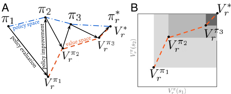
Fig. 1. (A) Sequence of policy updates as a trajectory that alternates between the policy and value spaces and eventually converges to an optimal solution (1). (B) Detailed view of the trajectory across the value space for a state space with two states only. The shadowed rectangles associated with each value function represent the region of the value space containing the value function that will result from one application of policy improvement followed by policy evaluation (cf. Exp. 2).

图 1: (A) 策略更新序列作为在策略空间和价值空间之间交替并最终收敛到最优解(1)的轨迹。(B) 仅包含两个状态的状态空间中,价值空间轨迹的详细视图。与每个价值函数关联的阴影矩形表示价值函数经过一次策略改进和策略评估后(参见实验2)将产生的价值空间区域。

Definition 4. Given a set of policies $\Pi$ and a task $r$ , “generalized policy improvement” (GPI) is the definition of a policy $\pi^{\prime}$ such that

定义 4. 给定策略集 $\Pi$ 和任务 $r$ ，"广义策略改进" (generalized policy improvement, GPI) 是指策略 $\pi^{\prime}$ 满足

$$
Q_{r}^{\pi^{\prime}}(s,a)\geq\operatorname*{sup}_ {\pi\in\Pi}Q_{r}^{\pi}(s,a)f o r a l l(s,a)\in S\times\mathcal A.
$$

$$
Q_{r}^{\pi^{\prime}}(s,a)\geq\operatorname*{sup}_ {\pi\in\Pi}Q_{r}^{\pi}(s,a) 对于所有 (s,a) \in S\times\mathcal A.
$$

GPE and GPI are strict generalizations of their standard counterparts, which are recovered when $\mathcal{R}$ has a single task and $\Pi$ has a single policy. However, it is when $\mathcal{R}$ and $\Pi$ are not singletons that GPE and GPI reach their full potential. In this case, they become a mechanism to quickly construct a solution for a task, as we now explain. Suppose we are interested in one of the tasks $r\in\mathcal{R}$ , and we have a set of policies $\Pi$ available. The origin of these policies is not important: they may have come up as solutions for specific tasks or have been defined in any other arbitrary way. If the policies $\pi\in\Pi$ are submitted to GPE, we have their value functions on the task $r\in\mathcal{R}$ . We can then apply GPI over these value functions to obtain a policy $\pi^{\prime}$ that represents an improvement over all policies in Π. Clearly, this reasoning applies without modification to any task in $\mathcal{R}$ . Therefore, by applying GPE and GPI to a set of policies $\Pi$ and a set of tasks $\mathcal{R}$ , one can compute a policy for any task in $\mathcal{R}$ that will in general outperform every policy in Π. Fig. 2 shows a graphical depiction of GPE and GPI.

GPE和GPI是其标准对应方法的严格泛化形式，当$\mathcal{R}$仅包含单个任务且$\Pi$仅包含单个策略时，它们将退化为标准形式。然而，只有当$\mathcal{R}$和$\Pi$不是单例集合时，GPE和GPI才能充分发挥潜力。此时，它们成为快速构建任务解决方案的机制，具体说明如下：假设我们关注任务集合$\mathcal{R}$中的某个任务$r\in\mathcal{R}$，并且拥有可用的策略集合$\Pi$。这些策略的来源并不重要——它们可能是针对特定任务的解决方案，也可能是通过任意其他方式定义的。若将策略$\pi\in\Pi$输入GPE，我们就能获得这些策略在任务$r\in\mathcal{R}$上的价值函数。随后可对这些价值函数应用GPI，得到优于$\Pi$中所有策略的新策略$\pi^{\prime}$。显然，该推理过程可原封不动地应用于$\mathcal{R}$中的任何任务。因此，通过对策略集合$\Pi$和任务集合$\mathcal{R}$应用GPE与GPI，可以为$\mathcal{R}$中的任何任务计算出普遍优于$\Pi$所有策略的新策略。图2展示了GPE和GPI的图示说明。

Obviously, in order for GPE and GPI to be useful in practice, we must have efficient ways of performing these operations. Consider GPE, for example. If we were to individually evaluate the policies $\pi\in\Pi$ over the set of tasks $r\in\mathcal{R}$ , it is unlikely that the scheme above would result in any gains in terms of computation or consumption of data. To see why this is so, suppose again that we are interested in a particular task $r$ . Computing the value functions of policies $\pi\in\Pi$ on task $r$ would require $\lceil\Pi\rceil$ policy evaluations with a naive form of GPE (here, $|\cdot|$ denotes the cardinality of a set). Although the resulting GPI policy $\pi^{\prime}$ would compare favorably to all policies in $\Pi$ , this guarantee would be vacuous if these policies are not competent at task $r$ . Therefore, a better allocation of resources might be to use the policy evaluations for standard policy updates, which would generate a sequence of $|\Pi|$ policies with increasing performance on task $r$ (compare Figs. 1 and 2). This difficulty in using generalized policy updates in practice is further aggravated if we do not have a fast way to carry out GPI. Next, we discuss efficient instantiations of GPE and GPI.

显然，要让GPE（广义策略评估）和GPI（广义策略改进）在实践中发挥作用，我们必须找到高效执行这些操作的方法。以GPE为例，如果我们对任务集$r\in\mathcal{R}$中的每个策略$\pi\in\Pi$单独进行评估，上述方案不太可能在计算或数据消耗方面带来任何增益。为了理解这一点，再次假设我们关注特定任务$r$。通过原始形式的GPE计算策略$\pi\in\Pi$在该任务上的价值函数，需要进行$|\Pi|$次策略评估（此处$|\cdot|$表示集合的基数）。尽管最终得到的GPI策略$\pi^{\prime}$会优于$\Pi$中的所有策略，但如果这些策略在任务$r$上表现不佳，这种保证将毫无意义。因此，更合理的资源分配可能是将这些策略评估用于标准策略更新，从而生成一系列在任务$r$上性能逐步提升的$|\Pi|$个策略（对比图1和图2）。如果我们没有快速执行GPI的方法，实践中使用广义策略更新的难度会进一步加剧。接下来，我们将讨论GPE和GPI的高效实现方案。

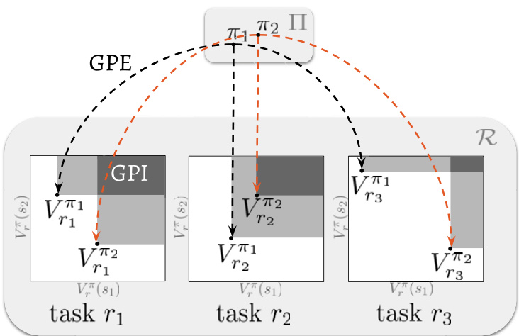
Fig. 2. Depiction of generalized policy updates on a state space with two states only. With GPE each policy $\pi\in\Pi$ is evaluated on all tasks $r\in\mathcal R$ . The state-value function of policy $\pi$ on task $r$ , $V_{r}^{\pi}$ , delimits a region in the value space where the next value function resulting from policy improvement will be (cf. Fig. 1). The analogous space induced by GPI corresponds to the intersection of the regions associated with the individual value functions (represented as dark gray rectangles in the figure). The smaller the space of value functions associated with GPI, the stronger the guarantees regarding the performance of the resulting policy.

图 2: 仅含两个状态的状态空间上广义策略更新的示意图。通过广义策略评估 (GPE) ，每个策略 $\pi\in\Pi$ 在所有任务 $r\in\mathcal R$ 上被评估。策略 $\pi$ 在任务 $r$ 上的状态价值函数 $V_{r}^{\pi}$ 界定了价值函数空间中策略改进后下一个价值函数所在的区域 (参见图 1) 。广义策略迭代 (GPI) 导出的类比空间对应于各个价值函数关联区域的交集 (图中以深灰色矩形表示) 。GPI 关联的价值函数空间越小，对最终策略性能的保证就越强。

Fast GPE with Successor Features. Conceptually, we can think of GPE as a function associated with a policy $\pi$ that takes a task $r$ as input and outputs a value function $Q_{r}^{\pi}$ (26). Hence, a practical way of implementing GPE would be to define a suitable representation for tasks and then learn a mapping from $r$ to value functions $Q_{r}^{\pi}$ (27). This is feasible when such a mapping can be reasonably approximated by the choice of function approx im at or and enough examples $(\dot{r},Q_{r}^{\pi})$ are available to characterize the relation underlying these pairs. Here, we will focus on a form of GPE that is based on a similar premise but leads to a form of generalization over tasks that is correct by definition.

基于后继特征的快速GPE。从概念上讲，我们可以将GPE视为与策略$\pi$相关联的函数，该函数以任务$r$作为输入并输出价值函数$Q_{r}^{\pi}$ (26)。因此，实现GPE的一种实用方法是定义合适的任务表示方法，然后学习从$r$到价值函数$Q_{r}^{\pi}$的映射 (27)。当这种映射能够通过函数逼近器的合理选择以及足够的样本$(\dot{r},Q_{r}^{\pi})$来表征这些对之间的潜在关系时，这是可行的。在这里，我们将重点讨论一种基于类似前提的GPE形式，但通过定义实现跨任务的正确泛化。

Let $\phi:\mathcal{S}\times\mathcal{A}\times\mathcal{S}\mapsto\mathbb{R}^{d}$ be an arbitrary function whose output we will see as “features.” Then, for any $\mathbf{w}\in\mathbb{R}^{d}$ , we have a task defined as

设 $\phi:\mathcal{S}\times\mathcal{A}\times\mathcal{S}\mapsto\mathbb{R}^{d}$ 为任意函数，其输出我们将视为"特征"。那么，对于任意 $\mathbf{w}\in\mathbb{R}^{d}$，我们定义如下任务：

$$
\begin{array}{r}{r_{\mathbf{w}}(s,a,s^{\prime})=\phi(s,a,s^{\prime})^{\top}\mathbf{w},}\end{array}
$$

where $\top$ denotes the transpose of a vector. Let

其中 $\top$ 表示向量的转置。设

$$
\mathcal{R}_ {\phi}\equiv{r_{\mathbf{w}}=\phi^{\top}\mathbf{w}|\mathbf{w}\in\mathbb{R}^{d}}
$$

Following Barreto et al. (28), we define the “successor features” (SFs) of policy $\pi$ as

根据 Barreto 等人的研究 [28]，我们将策略 $\pi$ 的“后继特征”(successor features，SFs)定义为

$$
\psi^{\pi}(s,a)\equiv\mathbb{E}^{\pi}\left[\sum_{i=0}^{\infty}\gamma^{i}\phi(S_{t+i},A_{t+i},S_{t+i+1})\mid S_{t}=s,A_{t}=a\right].
$$

The ith component of $\psi^{\pi}(s,a)$ gives the expected discounted sum of $\phi_{i}$ when following policy $\pi$ starting from $(s,a)$ . Thus, $\psi^{\pi}$ can be seen as a $d$ -dimensional value function in which the features $\phi_{i}(s,a,s^{\prime})$ play the role of reward functions (cf. Exp. 1). As a consequence, SFs satisfy a Bellman equation analogous to Exp. 3, which means that they can be computed using standard RL methods like temporal differences (22).

$\psi^{\pi}(s,a)$ 的第 $i$ 个分量表示从 $(s,a)$ 开始遵循策略 $\pi$ 时 $\phi_{i}$ 的期望折现和。因此，$\psi^{\pi}$ 可视为一个 $d$ 维价值函数，其中特征 $\phi_{i}(s,a,s^{\prime})$ 充当奖励函数的角色 (参见公式 1)。由此，成功特征 (SFs) 满足类似于公式 3 的贝尔曼方程，这意味着它们可通过时序差分等标准强化学习方法计算 [22]。

Given the SFs of a policy $\pi,\psi^{\pi}$ , we can quickly evaluate $\pi$ on task $r_{\mathbf{w}}\in\mathcal{R}_{\phi}$ by computing

给定策略$\pi,\psi^{\pi}$的SF (successor features) ，我们可以通过计算快速评估策略$\pi$在任务$r_{\mathbf{w}}\in\mathcal{R}_{\phi}$上的表现

$$
\begin{array}{r l r}{{\psi^{\pi}(s,a)^{\top}\mathbf{w}=\mathbb{E}^{\pi}\left[\displaystyle\sum_{i=0}^{\infty}\gamma^{i}\phi(S_{t+i},A_{t+i},S_{t+i+1})^{\top}\mathbf{w}|S_{t}=s,A_{t}=a\right]}}\ &{=\mathbb{E}^{\pi}\left[\displaystyle\sum_{i=0}^{\infty}\gamma^{i}r_{\mathbf{w}}(S_{t+i},A_{t+i},S_{t+i+1})\mid S_{t}=s,A_{t}=a\right]}\ &{=Q_{r_{\mathbf{w}}}^{\pi}(s,a)\equiv Q_{\mathbf{w}}^{\pi}(s,a).}&{[7]}\end{array}
$$

That is, the computation of the value function of policy $\pi$ on task $r_{\mathbf{w}}$ is reduced to the inner product $\psi^{\pi}(s,a)^{\top}\mathbf{w}$ . Since this is true for any task $r_{\mathbf{w}}$ , SFs provide a mechanism to implement a very efficient form of GPE over the set $\mathcal{R}_{\phi}$ (cf. Definition 3).

即，策略 $\pi$ 在任务 $r_{\mathbf{w}}$ 上的价值函数计算可简化为内积 $\psi^{\pi}(s,a)^{\top}\mathbf{w}$。由于这对任意任务 $r_{\mathbf{w}}$ 都成立，状态特征 (SFs) 提供了一种机制，可在集合 $\mathcal{R}_{\phi}$ 上实现非常高效的广义策略评估 (GPE) (参见定义 3)。

The question then arises as to how inclusive the set $\mathcal{R}_ {\phi}$ is. Since $\mathcal{R}_ {\phi}$ is fully determined by $\phi$ , the answer to this question lies in the definition of these features. Mathematically speaking, $\mathcal{R}_ {\phi}$ is the linear space spanned by the $d$ features $\phi_{i}$ . This view suggests ways of defining $\phi$ that result in a $\mathcal{R}_ {\phi}$ containing all possible tasks. A simple example can be given for when both the state space $s$ and the action space $\mathcal{A}$ are finite. In this case, we can recover any possible reward function by making $d=|S|^{2}\times|A|$ and having each $\phi_{i}$ be an indicator function associated with the occurrence of a specific transition $(s,a,s^{\prime})$ . This is essentially Dayan’s (29) concept of “successor representation” extended from $s$ to $S\times A\times S$ . The notion of covering the space of tasks can be generalized to continuous $s$ and $\mathcal{A}$ if we think of $\phi_{i}$ as basis functions over the function space $S\times\mathcal{A}\times\mathcal{S}\mapsto\mathbb{R}$ , for we know that, under some technical conditions, one can approximate any function in this space with arbitrary accuracy by having an appropriate basis.

问题随之而来：集合 $\mathcal{R}_ {\phi}$ 的包容性如何？由于 $\mathcal{R}_ {\phi}$ 完全由 $\phi$ 决定，这个问题的答案在于这些特征的定义。从数学上讲，$\mathcal{R}_ {\phi}$ 是由 $d$ 个特征 $\phi_{i}$ 张成的线性空间。这一观点提出了定义 $\phi$ 的方法，使得 $\mathcal{R}_ {\phi}$ 包含所有可能的任务。当状态空间 $s$ 和动作空间 $\mathcal{A}$ 均为有限时，可以给出一个简单示例：通过设定 $d=|S|^{2}\times|A|$ 并让每个 $\phi_{i}$ 成为特定转移 $(s,a,s^{\prime})$ 的指示函数，我们就能恢复任何可能的奖励函数。这本质上是 Dayan [29] 提出的“后继表示”概念从 $s$ 扩展到 $S\times A\times S$ 的结果。若将 $\phi_{i}$ 视为函数空间 $S\times\mathcal{A}\times\mathcal{S}\mapsto\mathbb{R}$ 上的基函数，任务空间覆盖的概念可推广至连续的 $s$ 和 $\mathcal{A}$ ——因为在某些技术条件下，通过适当的基函数可以任意精度逼近该空间中的任意函数。

Although these limiting cases are reassuring, more generally we want to have a number of features $\bar{d}\ll|S|$ . This is possible if we consider that we are only interested in a subset of all possible tasks—which should in fact be a reasonable assumption in most realistic scenarios. In this case, the features $\phi$ should capture the underlying structure of the set of tasks $\mathcal{R}$ in which we are interested. For example, many tasks we care about could be recovered by features $\phi_{i}$ representing entities (from concrete objects to abstract concepts) or salient events (such as the interaction between entities). In Fast $R L$ with GPE and $G P I$ , we give concrete examples of what the features $\phi$ may look like and also discuss possible ways of computing them directly from data. For now, it is worth mentioning that, even when $\phi$ does not span the space $\mathcal{R}$ , one can bound the error between the two sides of Exp. 7 based on how well the tasks of interest can be approximated using $\phi$ (proposition 1 in ref. 30).

虽然这些极限情况令人放心，但更普遍地我们希望满足特征数$\bar{d}\ll|S|$。如果我们只对所有可能任务的一个子集感兴趣——这实际上在大多数现实场景中都是合理假设，那么这一目标是可以实现的。此时，特征$\phi$应当能捕捉我们关注的任集$\mathcal{R}$的底层结构。例如，许多我们关心的任务可以通过表示实体（从具体对象到抽象概念）或显著事件（如实体间交互）的特征$\phi_{i}$来恢复。在《基于GPE和GPI的快速$RL$》中，我们给出了特征$\phi$的具体示例，并讨论了直接从数据计算它们的可能方法。目前值得指出的是，即使$\phi$未能张成空间$\mathcal{R}$，也可以根据感兴趣任务能被$\phi$逼近的程度，来约束表达式7两侧的误差（参考文献30中的命题1）。

Fast GPI with Value-Based Action Selection. Thanks to the concept of value function, standard policy improvement can be carried out efficiently through Exp. 4. This raises the question whether the same is possible with GPI. We now answer this question in the affirmative for the case in which GPI is applied over a finite set Π.

基于价值动作选择的快速GPI。得益于价值函数的概念，标准策略改进可以通过公式4高效实现。这引发了一个问题：GPI是否也能实现同样的效果？我们现在对GPI应用于有限集合Π的情况给出了肯定的答案。

Following Barreto et al. (28), we propose to compute an improved policy $\pi^{\prime}$ as

遵循 Barreto 等人的方法 [28]，我们提出计算改进策略 $\pi^{\prime}$ 为

$$
\pi^{\prime}(s)\in\underset{a\in\cal A}{\mathrm{argmax}}\operatorname*{max}_ {\pi\in\Pi}Q_{r}^{\pi}(s,a).
$$

Barreto et al. have shown that Exp. 8 qualifies as a legitimate form of GPI as per Definition 4 (theorem 1 in ref. 28). Note that the action selected by a GPI policy $\pi^{\prime}$ on a state $s$ may not coincide with any of the actions selected by the policies $\pi\in\Pi$ on that state. This highlights an important difference between Exp. 8 and methods that define a higher-level policy that alternates between the policies $\pi\in\Pi$ (32). In $S I$ Appendix, we show that the policy $\bar{\pi^{\prime}}$ resulting from Exp. 8 will in general outperform its analog defined over Π.

Barreto等人已证明，根据定义4 (定理1见文献[28]) ，实验8符合GPI的合法形式。需注意，GPI策略$\pi^{\prime}$在状态$s$下选择的动作，可能与策略集$\pi\in\Pi$中任一策略在该状态下选择的动作都不相同。这凸显了实验8与那些定义高层策略(在$\pi\in\Pi$间切换)的方法[32]之间的重要差异。在$SI$附录中，我们证明了实验8生成的策略$\bar{\pi^{\prime}}$通常优于定义在Π上的对应策略。

As discussed, GPI reduces to standard policy improvement when $\Pi$ contains a single policy. Interestingly, this also happens with Exp. 8 when one of the policies in $\bar{\Pi}$ strictly outperforms the others on task $r$ . This means that, after one application of GPI, adding the resulting policy $\pi^{\prime}$ to the set $\Pi$ will reduce the next application of Exp. 8 to Exp. 4. Therefore, if GPI is used in a sequence of policy updates, it will collapse back to its standard counterpart after the first update. In contrast with policy improvement, which is inherently iterative, GPI is an one-off operation that yields a quick solution for a task when multiple policies have been evaluated on it.

如前所述，当$\Pi$仅包含单一策略时，GPI (Generalized Policy Improvement) 会退化为标准策略改进。有趣的是，当$\bar{\Pi}$中某个策略在任务$r$上严格优于其他策略时，Exp. 8也会出现同样情况。这意味着，在应用一次GPI后，将所得策略$\pi^{\prime}$加入集合$\Pi$会使下一次Exp. 8退化为Exp. 4。因此，若在一系列策略更新中使用GPI，其将在首次更新后回归标准形式。与本质迭代的策略改进不同，GPI是一次性操作，当多个策略已在任务上完成评估时，它能快速生成解决方案。

The guarantees regarding the performance of the GPI policy $\pi^{\prime}$ can be extended to the scenario where Exp. 8 is used with approximate value functions. In this case, the lower bound in Exp. 5 decreases in proportion to the maximum approximation error in the value function approximations (theorem 1 in ref. 28). We refer the reader to $S I$ Appendix for an extended discussion on GPI.

关于GPI策略$\pi^{\prime}$性能的保证可以扩展到Exp. 8与近似值函数结合使用的情况。此时，Exp. 5中的下界会随着值函数近似中的最大近似误差成比例降低(参考文献28中的定理1)。关于GPI的扩展讨论，请读者参阅$SI$附录。

The Generalized Policy. Strictly speaking, in order to leverage the instantiations of GPE and GPI discussed in this article, we only need two elements: features $\phi:S\times\mathcal{A}\times\mathcal{S}\mapsto\mathbb{R}^{d}$ and a set of policies $\Pi={\pi_{i}}_ {i=1}^{n}$ . Together, these components yield a set of SFs $\Psi={\psi^{\pi_{i}}}_ {i=1}^{n}$ , which provide a quick form of GPE over the set of tasks $\mathcal{R}_ {\phi}$ induced by the features $\phi$ . Specifically, for any $\mathbf{w}\in\mathbb{R}^{d}$ , we can quickly evaluate policy $\pi_{i}$ on task $r_{\mathbf{w}}(s,a,s^{\prime})=$ $\phi(s,a,s^{\prime})^{\top}\mathbf{w}$ by computing $Q_{\mathbf{w}}^{\pi_{i}}(s,a)=\psi^{\pi_{i}}(s,a)^{\top}\mathbf{w}$ . Once we have the value functions of policies $\pi_{i}$ on task $r_{\mathbf{w}}$ , $\left{Q_{\mathbf{w}}^{\pi_{i}}\right}_ {i=1}^{n}$ , Exp. 8 can be used to obtain a GPI policy $\pi^{\prime}$ that will in general outperform the policies $\pi_{i}$ on $r_{\mathbf{w}}$ . Observe that the same scheme can be used if we have approximate SFs $\tilde{\psi}^{\pi_{i}}\approx\psi^{\pi_{i}}$ , which will be the case in most realistic scenarios. Since the resulting value functions will also be approximations, $\tilde{Q}_ {\mathbf{w}}^{\pi_{i}}\approx Q_{\mathbf{w}}^{\pi_{i}}$ , we are back to the approximate version of GPI discussed in Fast GPI with Value-Based Action Selection.

广义策略。严格来说，为了利用本文讨论的GPE和GPI实例化，我们只需要两个要素：特征$\phi:S\times\mathcal{A}\times\mathcal{S}\mapsto\mathbb{R}^{d}$和策略集合$\Pi={\pi_{i}}_ {i=1}^{n}$。这些组件共同产生一组SF$\Psi={\psi^{\pi_{i}}}_ {i=1}^{n}$，为特征$\phi$导出的任务集合$\mathcal{R}_ {\phi}$提供了一种快速的GPE形式。具体来说，对于任何$\mathbf{w}\in\mathbb{R}^{d}$，我们可以通过计算$Q_{\mathbf{w}}^{\pi_{i}}(s,a)=\psi^{\pi_{i}}(s,a)^{\top}\mathbf{w}$来快速评估策略$\pi_{i}$在任务$r_{\mathbf{w}}(s,a,s^{\prime})=\phi(s,a,s^{\prime})^{\top}\mathbf{w}$上的表现。一旦我们获得了策略$\pi_{i}$在任务$r_{\mathbf{w}}$上的价值函数$\left{Q_{\mathbf{w}}^{\pi_{i}}\right}_ {i=1}^{n}$，就可以使用表达式8来获得一个GPI策略$\pi^{\prime}$，该策略通常会在$r_{\mathbf{w}}$上优于策略$\pi_{i}$。需要注意的是，如果我们有近似SF$\tilde{\psi}^{\pi_{i}}\approx\psi^{\pi_{i}}$，也可以使用相同的方案，这在大多数实际场景中都是如此。由于得到的价值函数也将是近似值$\tilde{Q}_ {\mathbf{w}}^{\pi_{i}}\approx Q_{\mathbf{w}}^{\pi_{i}}$，我们回到了基于值动作选择的快速GPI中讨论的GPI近似版本。

Given a set of SFs $\Psi$ , approximate or otherwise, any $\mathbf{w}\in\mathbb{R}^{d}$ gives rise to a policy through GPE (Exp. 7) and GPI (Exp. 8). We can thus think of generalized updates as implementing a policy $\pi_{\Psi}(s;\mathbf{w})$ whose behavior is modulated by w. We will call $\pi\Psi$ a “generalized policy.” Fig. 3 provides a schematic view of the computation of $\pi\Psi$ through GPE and GPI.

给定一组SF $\Psi$（近似或其他形式），任何$\mathbf{w}\in\mathbb{R}^{d}$都能通过广义策略评估(GPE)（式7）和广义策略改进(GPI)（式8）生成一个策略。因此，我们可以将广义更新视为实现了一个行为由w调控的策略$\pi_{\Psi}(s;\mathbf{w})$。我们将$\pi\Psi$称为"广义策略"。图3展示了通过GPE和GPI计算$\pi\Psi$的示意图。

Since each component of w weighs one of the features $\phi_{i}(s,a,s^{\prime})$ , changing them can intuitively be seen as setting the agent’s current “preferences.” For example, the vector $\mathbf{w}=$ $[0,1,-2]^{\top}$ indicates that the agent is in different to feature $\phi_{1}$ and wants to seek feature $\phi_{2}$ while avoiding feature $\phi_{3}$ with twice the impetus. Specific instantiations of $\pi\Psi$ can behave in ways that are very different from its constituent policies $\pi\in\Pi$ . We can draw a parallel with nature if we think of features as concepts like water or food and note how much the desire for these items can affect an animal’s behavior. Analogies aside, this sort of arithmetic over features provides a rich interface for the agent to interact with the environment at a higher level of abstraction in which decisions correspond to preferences encoded as a vector w. Next, we discuss how this can be leveraged to speed up the solution of an RL task.

由于向量 w 的每个分量都对特征 $\phi_{i}(s,a,s^{\prime})$ 进行加权，调整这些分量可直观理解为设置智能体的当前"偏好"。例如，向量 $\mathbf{w}=$ $[0,1,-2]^{\top}$ 表示该智能体对特征 $\phi_{1}$ 持中立态度，追求特征 $\phi_{2}$ 的同时以双倍动力规避特征 $\phi_{3}$。策略 $\pi\Psi$ 的具体实例可能表现出与原始策略集 $\pi\in\Pi$ 截然不同的行为模式。若将特征类比为水或食物等自然概念，并观察这些需求如何影响动物行为，便能建立直观理解。抛开类比不谈，这种特征层面的算术运算为智能体提供了更高抽象层次的交互接口，其决策对应于以向量 w 编码的偏好设定。接下来我们将探讨如何利用该机制加速强化学习任务的求解。

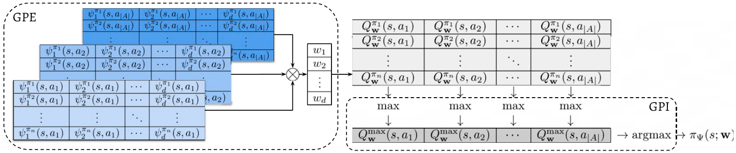
Fig. 3. Schematic representation of how the generalized policy $\pi\Psi$ is implemented through GPE and GPI. Given a state $s\in S$ , the first step is to compute, for each $a\in{\mathcal{A}}$ , the values of the $n$ SFs: ${\psi^{\pi}\mathfrak{i}(s,a)}_ {i=1}^{n}$ . Note that $\psi^{\pi_{j}}$ can be arbitrary nonlinear functions of their inputs, possibly represented by complex ap proxima tors like deep neural networks (30, 31). The SFs can be laid out as an $n\times|{\cal A}|\times d$ tensor in which the entry $(j,a,j)$ is ${\psi}_ {j}^{\pi_{i}}(s,a)$ . Given this layout, GPE reduces to the multiplication of the SF tensor with a vector $\mathbf{w}\in\mathbb{R}^{d}$ , the result of which is an $n\times|A|$ matrix whose $(i,a)$ entry is $Q^{\pi_{i}}(s,a)$ . GPI then consists in finding the maximum element of this matrix and returning the associated action a. This whole process can be seen as the implementation of a policy $\pi_{\Psi}(s;{\mathbf w})$ whose behavior is parameterized by a vector of preferences w.

图 3: 通过GPE和GPI实现广义策略$\pi\Psi$的示意图。给定状态$s\in S$，第一步是为每个$a\in{\mathcal{A}}$计算$n$个SF的值：${\psi^{\pi}\mathfrak{i}(s,a)}_ {i=1}^{n}$。注意$\psi^{\pi_{j}}$可以是其输入的任意非线性函数，可能由深度神经网络等复杂近似器表示[30, 31]。这些SF可以排列成一个$n\times|{\cal A}|\times d$张量，其中条目$(j,a,j)$为${\psi}_ {j}^{\pi_{i}}(s,a)$。基于这种布局，GPE简化为将SF张量与向量$\mathbf{w}\in\mathbb{R}^{d}$相乘，结果得到一个$n\times|A|$矩阵，其$(i,a)$条目为$Q^{\pi_{i}}(s,a)$。GPI则是在该矩阵中寻找最大元素并返回关联动作a。整个过程可视为策略$\pi_{\Psi}(s;{\mathbf w})$的实现，其行为由偏好向量w参数化。

Fast RL with GPE and GPI

基于GPE和GPI的快速强化学习

We now describe how to build and use the adaptable policy $\pi\Psi$ implemented by GPE and GPI. To make the discussion more concrete, we consider a simple RL environment depicted in Fig. 4. The environment consists of a $10\times10$ grid with four actions available: ${\mathcal{A}}={\mathfrak{u p}$ , down, left, right}. The agent occupies one of the grid cells, and there are also 10 objects spread across the grid. Each object belongs to one of two types. At each time step $t$ , the agent receives an image showing its position and the position and type of each object. Based on this information, the agent selects an action $a\in{\mathcal{A}}$ , which moves it one cell along the desired direction. The agent can pick up an object by moving to the cell occupied by it; in this case, it gets a reward defined by the type of the object. A new object then pops up in the grid, with both its type and location sampled uniformly at random (more details are in SI Appendix).

我们现在描述如何构建和使用由GPE和GPI实现的可适应策略$\pi\Psi$。为了使讨论更具体，我们考虑图4中描述的一个简单RL环境。该环境由一个$10\times10$的网格组成，提供四种动作：${\mathcal{A}}={\mathfrak{u p}$、down、left、right}。智能体占据网格中的一个单元格，同时还有10个物体分布在网格上。每个物体属于两种类型之一。在每个时间步$t$，智能体接收到一张图像，显示其位置以及每个物体的位置和类型。基于这些信息，智能体选择一个动作$a\in{\mathcal{A}}$，使其沿所需方向移动一格。智能体可以通过移动到物体所在的单元格来拾取物体；此时，它会获得由物体类型定义的奖励。随后，一个新物体会在网格中随机出现，其类型和位置均均匀随机采样（更多细节见SI附录）。

This simple environment can be seen as a prototypical member of the class of problems in which GPE and GPI could be useful. This becomes clear if we think of objects as instances of (potentially abstract) concepts, here symbolized by their types, and note that the navigation dynamics are a proxy for any sort of dynamics that mediate the interaction of the agent with the world. In addition, despite its small size, the number of possible configurations of the grid is actually quite large, of the order of $10^{15}$ . This precludes an exact representation of value functions and illustrates the need for approximations that inevitably arises in many realistic scenarios.

这个简单环境可视为GPE和GPI适用问题类别的原型范例。若将对象视为(潜在抽象)概念的实例(此处用类型符号表示)，并注意到导航动态是AI智能体与世界交互的任何动态过程的代理，这一点就变得显而易见。此外，尽管网格规模很小，但其可能配置的数量级实际上高达$10^{15}$，这排除了价值函数的精确表示，也说明了在许多现实场景中不可避免需要近似方法。

By changing the rewards associated with each object type, one can create different tasks. We will consider that the agent wants to build a set of SFs $\Psi$ that give rise to a generalized policy $\pi_{\Psi}(s;\mathbf{w})$ that can adapt to different tasks through the vector of preferences w. This can be either because the agent does not know in advance the task it will face or because it will face more than one task.

通过改变与每种对象类型相关的奖励，可以创建不同的任务。我们将考虑智能体希望构建一组能产生广义策略 $\pi_{\Psi}(s;\mathbf{w})$ 的状态特征 (SF) $\Psi$，该策略可通过偏好向量 w 适应不同任务。这可能是因为智能体事先不知道它将面临的任务，或者因为它将面临多个任务。

Defining a Basis for Behavior. In order to build the SFs $\Psi$ , the agent must define two things: features $\phi$ and a set of policies $\Pi$ . Since $\phi$ should be associated with rewarding events, we define each feature $\phi_{i}$ as an indicator function signaling whether an object of type $i$ has been picked up by the agent (i.e., $\phi\in\mathbb{R}^{2}$ ). To be precise, we have that $\phi_{i}(s,a,s^{\prime}){=}1$ if the transition from state $s$ to state $s^{\prime}$ is associated with the agent picking up an object of type $i$ , and $\phi_{i}(s,a,s^{\prime})=0$ otherwise. These features induce a set $\mathcal{R}_ {\phi}$ where task $r_{\mathbf{w}}\in\mathcal{R}_{\phi}$ is characterized by how desirable or undesirable each type of object is.

定义行为基础。为了构建SF $\Psi$，智能体需要定义两个要素：特征 $\phi$ 和策略集 $\Pi$。由于 $\phi$ 应与奖励事件相关联，我们将每个特征 $\phi_{i}$ 定义为指示函数，用于判断智能体是否拾取了类型 $i$ 的对象（即 $\phi\in\mathbb{R}^{2}$）。具体而言，当状态从 $s$ 转移到 $s^{\prime}$ 且涉及拾取类型 $i$ 的对象时，$\phi_{i}(s,a,s^{\prime}){=}1$；否则 $\phi_{i}(s,a,s^{\prime})=0$。这些特征导出一个集合 $\mathcal{R}{\phi}$，其中任务 $r{\mathbf{w}}\in\mathcal{R}_{\phi}$ 由每类对象的可取程度决定。

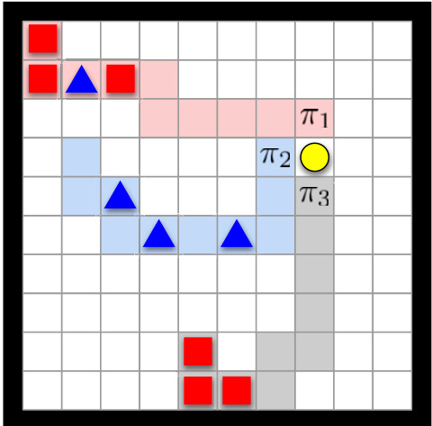
Fig. 4. Depiction of the environment used in the experiments. The shape of the objects (square or triangle) represents their type; the agent is depicted as a circle. We also show the first 10 steps taken by 3 policies, $\pi_{1},\pi_{2} $ , and $\pi_{3}$ , that would perform optimally on tasks $\mathbf{w}_ {1}=[1,0]$ , $\mathsf{w}_ {2}=[0,1]$ , and ${\bf w}_{3}=$ $[1,-1]$ for any discount factor $\gamma\geq0.5$ .

图 4: 实验中使用的环境示意图。物体形状(方形或三角形)代表其类型；智能体以圆形表示。我们还展示了三种策略 $\pi_{1},\pi_{2}$ 和 $\pi_{3}$ 的前10步行动轨迹，这些策略分别在任务 $\mathbf{w}_ {1}=[1,0]$ 、$\mathsf{w}_ {2}=[0,1]$ 和 ${\bf w}_{3}=[1,-1]$ 上对任何折扣因子 $\gamma\geq0.5$ 都能达到最优表现。

Now that we have defined $\phi$ , we turn to the question of how to determine an appropriate set of policies $\Pi$ . We will restrict the policies in $\Pi$ to be solutions to tasks $r_{\mathbf{w}}\in\mathcal{R}_ {\phi}$ . We start with what is perhaps the simplest choice in this case: a set $\Pi_{12}={\pi_{1},\pi_{2}}$ whose two elements are solutions to the tasks $\mathbf{w}_ {1}=\left[1,0\right]^{\top}$ and $\mathbf{w}_ {2}=[0,1]^{\top}$ (henceforth, we will drop the transpose superscript to avoid clutter). Note that the goal in tasks ${\bf w}_ {1}$ and $\mathbf{w}_{2}$ is to pick up objects of one type while ignoring objects of the other type.

既然我们已经定义了 $\phi$，接下来要解决的问题是如何确定一个合适的策略集 $\Pi$。我们将限制 $\Pi$ 中的策略为任务 $r_{\mathbf{w}}\in\mathcal{R}_ {\phi}$ 的解决方案。首先考虑这种情况下最简单的选择：一个由 $\Pi_{12}={\pi_{1},\pi_{2}}$ 组成的集合，其中两个元素分别是任务 $\mathbf{w}_ {1}=\left[1,0\right]^{\top}$ 和 $\mathbf{w}_ {2}=[0,1]^{\top}$ 的解决方案（为简洁起见，后续将省略转置上标）。需要注意的是，任务 ${\bf w}_ {1}$ 和 $\mathbf{w}_{2}$ 的目标是拾取一种类型的物体而忽略另一种类型的物体。

We are now ready to compute the SFs $\Psi$ induced by our choices of $\phi$ and $\Pi$ . In our experiments, we used an algorithm analogous to $Q$ -learning to compute approximate SFs $\bar{\psi}^{\pi_{1}}$ and $\tilde{\psi}^{\pi_{2}}$ (pseudocode in SI Appendix). We represented the SFs using multilayer perce ptr on s with two hidden layers (33).

我们现在可以计算由选择的 $\phi$ 和 $\Pi$ 所诱导的 SFs $\Psi$。实验中，我们采用了类似 $Q$ 学习 (Q-learning) 的算法来计算近似 SFs $\bar{\psi}^{\pi_{1}}$ 和 $\tilde{\psi}^{\pi_{2}}$ (伪代码见 SI附录)。SFs 使用具有两个隐藏层的多层感知器 (multilayer perceptron) 表示 [33]。

The set of SFs $\tilde{\Psi}$ yields a generalized policy $\pi_{\tilde{\Psi}}(s;\mathbf{w})$ parameterized by w. We now evaluate $\pi_{\tilde{\Psi}}$ on the task whose goal is to pick up objects of the first type while avoiding objects of the second type. Using $\phi$ defined above, this task can be represented as $\bar{r_{\mathbf{w}_ {3}}}(s,a,s^{\prime})=\phi(s,a,s^{\prime})^{\top}\mathbf{w}_ {3}$ , with $\mathbf{w}_ {3}=[1,-1]$ . We thus evaluate the generalized policy instantiated as $\pi_{\tilde{\Psi}}(s;{\bf w}_{3})$ .

SF集合 $\tilde{\Psi}$ 生成一个由w参数化的广义策略 $\pi_{\tilde{\Psi}}(s;\mathbf{w})$。我们现在评估 $\pi_{\tilde{\Psi}}$ 在以下任务上的表现：该任务目标是拾取第一类物体并避开第二类物体。使用上述定义的 $\phi$，该任务可表示为 $\bar{r_{\mathbf{w}_ {3}}}(s,a,s^{\prime})=\phi(s,a,s^{\prime})^{\top}\mathbf{w}_ {3}$，其中 $\mathbf{w}_ {3}=[1,-1]$。因此我们评估实例化为 $\pi_{\tilde{\Psi}}(s;{\bf w}_{3})$ 的广义策略。

Results are shown in Fig. 5A. As a reference, we also show the learning curve of $Q$ -learning (23) using the same architecture to directly approximate $Q_{\mathbf{w}_ {3}}^{\pi}$ . GPE and GPI allow one to compute an instantaneous solution for a new task, without any learning on the task itself, that is competitive with the policies found by $Q$ -learning when using around $6\times10^{4}$ sample transitions. The performance of the policy $\pi_{\tilde{\Psi}}$ synthesized by GPE and GPI corresponds to more than $70%$ of the performance eventually achieved by $Q$ -learning after processing $10^{6}$ transitions. This is quite an impressive result when we note that $\pi_{\tilde{\Psi}}$ managed to avoid objects of the second type even though its constituents policies $\pi_{1}$ and $\pi_{2}$ were never trained to actively avoid objects.

结果如图5A所示。作为参考，我们还展示了使用相同架构直接逼近 $Q_{\mathbf{w}_ {3}}^{\pi}$ 的 $Q$ -学习(23)的学习曲线。GPE和GPI允许为新任务计算即时解，无需任务本身的学习，其性能与 $Q$ -学习使用约 $6\times10^{4}$ 样本转移时找到的策略相当。由GPE和GPI合成的策略 $\pi_{\tilde{\Psi}}$ 的性能达到了 $Q$ -学习处理 $10^{6}$ 次转移后最终性能的70%以上。值得注意的是，尽管其组成策略 $\pi_{1}$ 和 $\pi_{2}$ 从未被训练主动避开物体， $\pi_{\tilde{\Psi}}$ 仍成功避开了第二类物体，这一结果令人印象深刻。

We used a total of $10^{6}$ sample transitions to learn both SFs $\tilde{\psi}^{\pi_{1}}$ and $\tilde{\psi}^{\pi_{2}}$ , which is the same amount of data used by $Q$ learning to achieve its final performance. The advantage of doing the former is that, once we have the SFs, we can use GPE and GPI to instantaneously compute a solution for any task in $\mathcal{R}_ {\phi}$ . However, how well do GPE and GPI actually perform on $\mathcal{R}_ {\phi}$ ? To answer this question, we ran a second round of experiments to assess the generalization of $\pi_{\tilde{\Psi}}$ over the entire set $\mathcal{R}_ {\phi}$ . Since this evaluation clearly depends on the set of policies used, we consider two other sets in addition to $\Pi_{12}={{\bar{\pi}}_ {1},\pi_{2}}$ . The new sets are $\Pi_{34}={\pi_{3},\pi_{4}}$ and $\Pi_{5}={\pi_{5}}$ , where the policies $\pi_{i}$ are solutions to the tasks $\mathbf{w}_ {3}=\left[1,-1\right]$ , $\mathbf{w}_ {4}=[-1,1]$ , and $\mathbf{w}_ {5}=[1,1]$ . We repeated the previous experiment with each policy set and evaluated the resulting policies $\pi_{\tilde{\Psi}}$ over 19 tasks $\mathbf{w}$ evenly spread over the non negative quadrants of the unit circle (tasks in the negative quadrant are uninteresting because all of the agent must do is to avoid hitting objects). Results are shown in Fig. 6A. As expected, the generalization ability of GPE and GPI depends on the set of policies used. Perhaps more surprising is how well the generalized policy $\pi_{\tilde{\Psi}}$ induced by some of these sets perform across the entire space of tasks $\mathcal{R}_{\phi}$ , sometimes matching the best performance of $Q$ -learning when solving each task individually.

我们总共使用了 $10^{6}$ 个样本转移来学习 $\tilde{\psi}^{\pi_{1}}$ 和 $\tilde{\psi}^{\pi_{2}}$，这与 $Q$ 学习达到最终性能时使用的数据量相同。前者的优势在于，一旦我们获得了这些 SFs (Successor Features)，就可以使用 GPE (Generalized Policy Evaluation) 和 GPI (Generalized Policy Improvement) 即时计算 $\mathcal{R}_ {\phi}$ 中任何任务的解决方案。然而，GPE 和 GPI 在 $\mathcal{R}_ {\phi}$ 上的实际表现如何？为了回答这个问题，我们进行了第二轮实验，评估 $\pi_{\tilde{\Psi}}$ 在整个 $\mathcal{R}_ {\phi}$ 集合上的泛化能力。由于这一评估显然依赖于所使用的策略集，除了 $\Pi_{12}={{\bar{\pi}}_ {1},\pi_{2}}$ 外，我们还考虑了另外两个集合：$\Pi_{34}={\pi_{3},\pi_{4}}$ 和 $\Pi_{5}={\pi_{5}}$，其中策略 $\pi_{i}$ 分别对应任务 $\mathbf{w}_ {3}=\left[1,-1\right]$、$\mathbf{w}_ {4}=[-1,1]$ 和 $\mathbf{w}_ {5}=[1,1]$ 的解决方案。我们对每个策略集重复了之前的实验，并在单位圆非负象限上均匀分布的 19 个任务 $\mathbf{w}$ 上评估了生成的策略 $\pi_{\tilde{\Psi}}$（负象限的任务无意义，因为智能体只需避免碰撞物体）。结果如图 6A 所示。正如预期，GPE 和 GPI 的泛化能力取决于所使用的策略集。更令人惊讶的是，某些策略集诱导的广义策略 $\pi_{\tilde{\Psi}}$ 在整个任务空间 $\mathcal{R}_{\phi}$ 中的表现，有时甚至与单独解决每个任务时 $Q$ 学习的最佳性能相当。

These experiments show that a proper choice of base policies $\Pi$ can lead to good generalization over the entire set of tasks $\mathcal{R}_ {\phi}$ . In general, though, it is unclear how to define an appropriate Π. Fortunately, we can refer to our theoretical understanding of GPE and GPI to have some guidance. First, we know from the discussion above that the larger the number of policies in $\Pi$ the stronger the guarantees regarding the performance of the resulting policy $\pi_{\tilde{\Psi}}$ (Exp. 5). In addition to that, Barreto et al. have shown that it is possible to guarantee a minimum performance level for $\pi_{\tilde{\Psi}}$ on task $\mathbf{w}$ based on $\operatorname*{min}_ {i}|\mathbf{w}-\mathbf{w}_ {i}|$ , where $|\cdot|$ is some norm and $\mathbf{w}_ {i}$ are the tasks associated with the policies $\pi_{i}\in\Pi$ used for GPE and GPI (theorem 2 in ref. 28). Together, these two insights suggest that, as we increase the size of $\Pi$ , the performance of the resulting policy $\pi_{\tilde{\Psi}}$ should improve across $\mathcal{R}_ {\phi}$ , especially on tasks that are close to the tasks $\mathbf{w}_ {i}$ . To test this hypothesis empirically, we repeated the previous experiment, but now, instead of comparing disjoint policy sets, we compared a sequence of sets formed by adding one by one the policies $\pi_{2}$ , $\pi_{5}$ , $\pi_{1}$ , and $\pi_{3}$ , in this order, to the initial set ${\pi_{4}}$ . The results, in Fig. $6B$ , confirm the trend implied by the theory.

这些实验表明，基础策略集 $\Pi$ 的合理选择能促进任务集 $\mathcal{R}_ {\phi}$ 上的良好泛化能力。然而，通常难以明确定义合适的 $\Pi$。幸运的是，我们可以参考对GPE（广义策略评估）和GPI（广义策略迭代）的理论理解来获得指导。首先，前文讨论表明 $\Pi$ 中包含的策略越多，最终策略 $\pi_{\tilde{\Psi}}$ 的性能保证就越强（公式5）。此外，Barreto等人[28]证明，基于 $\operatorname*{min}_ {i}|\mathbf{w}-\mathbf{w}_ {i}|$ （其中 $|\cdot|$ 为某种范数，$\mathbf{w}_ {i}$ 是与GPE/GPI所用策略 $\pi_{i}\in\Pi$ 关联的任务），可确保 $\pi_{\tilde{\Psi}}$ 在任务 $\mathbf{w}$ 上的最低性能水平（文献28定理2）。这两点共同表明：随着 $\Pi$ 规模扩大，最终策略 $\pi_{\tilde{\Psi}}$ 在 $\mathcal{R}_ {\phi}$ 上的性能应会提升，尤其在接近 $\mathbf{w}_ {i}$ 的任务上。为实证验证该假设，我们重复前述实验，但改为比较逐步扩充的策略集：在初始集 ${\pi_{4}}$ 基础上，依次添加 $\pi_{2}$、$\pi_{5}$、$\pi_{1}$ 和 $\pi_{3}$。图6B的结果印证了理论预测的趋势。

Fig. 5. Average sum of rewards on task $\mathbf{w}_ {3}=[1,-1]$ . GPE and GPI used $\Pi_{12}={\pi_{1},\pi_{2}}$ as the base policies and the corresponding SFs consumed $5\times10^{5}$ sample transitions to be trained each. $B$ is a zoomed-in version of A showing the early performance of GPE and GPI under different setups. The results reflect the best performance of each algorithm over multiple parameter configurations (SI Appendix). Shadowed regions are one standard error over 100 runs.

图 5: 任务 $\mathbf{w}_ {3}=[1,-1]$ 上的平均奖励总和。GPE 和 GPI 使用 $\Pi_{12}={\pi_{1},\pi_{2}}$ 作为基础策略，对应的 SFs 各消耗 $5\times10^{5}$ 个样本转移进行训练。$B$ 是 $A$ 的放大版本，展示了不同设置下 GPE 和 GPI 的早期性能。结果反映了每种算法在多个参数配置下的最佳表现 (SI附录)。阴影区域为100次运行的一个标准误差。

Task Inference. So far, we have assumed that the agent knows the vector w that describes the task of interest. Although this can be the case in some scenarios, ideally we would be able to apply GPE and GPI even when w is not provided. In this section and in Preferences as Actions, we describe two possible ways for the agent to learn w.

任务推断。到目前为止，我们假设智能体已知描述目标任务的向量w。虽然某些场景下确实如此，但理想情况下即使未提供w，我们仍应能应用GPE(广义策略评估)和GPI(广义策略改进)。本节及"偏好即行动"章节中，我们将阐述智能体学习w的两种可行方法。

Given a task $r$ , we are looking for a $\mathbf{w}\in\mathbb{R}^{d}$ that leads to good performance of the generalized policy $\pi_{\Psi}(s;\mathbf{w})$ . We could in principle approach this problem as an optimization over $\mathbf{w}\in\mathbb{R}^{d}$ whose objective is to maximize the value of $\pi_{\Psi}(s;\mathbf{w})$ across (a subset of) the state space. It turns out that we can exploit the structure underlying SFs to efficiently determine w without ever looking at the value of $\pi\Psi$ . Suppose we have a set of $m$ sample transitions from a given task, ${(s_{i},a_{i},r_{i}^{\prime},s_{i}^{\prime})}_{i=1}^{m}$ . Then, based on Exp. 6, we can infer w by solving the following minimization:

给定任务 $r$，我们寻找一个能使得广义策略 $\pi_{\Psi}(s;\mathbf{w})$ 表现良好的 $\mathbf{w}\in\mathbb{R}^{d}$。原则上，我们可以将此问题转化为对 $\mathbf{w}\in\mathbb{R}^{d}$ 的优化，其目标是在状态空间（的子集）上最大化 $\pi_{\Psi}(s;\mathbf{w})$ 的值。事实证明，我们可以利用后继特征（SFs）的底层结构来高效确定 $\mathbf{w}$，而无需考察 $\pi_{\Psi}$ 的值。假设我们有一组来自给定任务的 $m$ 个样本转移 ${(s_{i},a_{i},r_{i}^{\prime},s_{i}^{\prime})}_{i=1}^{m}$，那么基于公式 6，我们可以通过求解以下最小化问题来推断 $\mathbf{w}$：

$$
\operatorname*{min}_ {\tilde{\mathbf{w}}}\sum_{i=1}^{m}|\phi(s_{i},a_{i},s_{i}^{\prime})^{\top}\tilde{\mathbf{w}}-r_{i}^{\prime}|^{p},
$$

where $p\geq1$ (one may also want to consider the inclusion of a regular iz ation term, see ref. 33). Observe that, once we have a solution $\tilde{\bf w}$ for the problem above, we can plug it in Exp. 7 and use GPE and GPI as we did before—that is, we have just turned an RL task into an easier linear regression problem.

其中 $p\geq1$ (也可以考虑加入正则化项，参见文献 [33])。注意到，一旦我们得到上述问题的解 $\tilde{\bf w}$，就可以将其代入表达式 7，并像之前那样使用 GPE 和 GPI——也就是说，我们刚刚将一个强化学习任务转化为了更简单的线性回归问题。

To illustrate the potential of this approach, we revisited the task $\mathbf{w}_ {3}=[1,-1]$ tackled above, but now, instead of assuming we knew ${\bf w}_ {3}$ , we solved the problem in Exp. 9 using $p=2$ . We collected sample transitions using a policy $\hat{\pi}$ that picks actions uniformly at random and used the gradient descent method to refine an approximation $\tilde{\mathbf{w}}\approx\mathbf{w}$ online (SI Appendix). Results are shown in Fig. $5A$ and $B$ . The performance of the generalized policy $\pi_{\tilde{\Psi}}(s;{\bf w}_ {3})$ using the correct $\mathbf{w}_{3}$ was recovered after around 800 sample transitions only. To put this number into perspective, recall that $Q$ -learning needs around 60,000 transitions, or 75 times as much data, to achieve the same performance level. The number of transitions needed to learn w can be reduced further if we use the closed-form solution for the least-squares problem.

为了说明这种方法的潜力，我们重新审视了之前处理的任务 $\mathbf{w}_ {3}=[1,-1]$，但这次不再假设已知 ${\bf w}_ {3}$，而是在实验9中使用 $p=2$ 来求解该问题。我们通过随机均匀选择动作的策略 $\hat{\pi}$ 收集样本转移数据，并采用梯度下降法在线优化近似值 $\tilde{\mathbf{w}}\approx\mathbf{w}$（详见SI附录）。结果如图 $5A$ 和 $B$ 所示。使用正确 $\mathbf{w}_ {3}$ 的广义策略 $\pi_{\tilde{\Psi}}(s;{\bf w}_{3})$ 仅需约800次样本转移就恢复了原有性能。作为对比，$Q$-学习需要约60,000次转移（即75倍数据量）才能达到相同性能水平。若采用最小二乘问题的闭式解，学习w所需的转移次数还可进一步减少。

Fig. 6. Results on the space of tasks $\mathcal{R}_{\phi}$ induced by a two-dimensional $\phi$ . The sets of policies Π used in A are disjoint; in B these sets overlap. The evaluation of an algorithm on a task is represented as a vector whose direction indicates the task w and whose magnitude gives the average sum of rewards over 10 runs with 250 trials each. $Q$ -learning learned each task individually, from scratch; the dotted curves correspond to its performance after having processed $5\times10^{4}$ , $1\times10^{5}$ , $2\times10^{5}$ , $5\times10^{5}$ , and $1\times10^{6}$ sample transitions. Our method only learned the policies in the sets Π and then generalized across all others tasks through GPE and GPI. The SFs used for GPE and GPI consumed $5\times10^{5}$ sample transitions to be trained each.

图 6: 二维参数 $\phi$ 诱导的任务空间 $\mathcal{R}_{\phi}$ 上的结果。A组使用的策略集Π互不相交；B组中这些策略集存在重叠。算法在任务上的评估结果表示为向量，其方向表示任务w，长度表示10次运行（每次250次试验）的平均累计奖励。$Q$-learning从零开始独立学习每个任务；虚线曲线对应其处理 $5\times10^{4}$、$1\times10^{5}$、$2\times10^{5}$、$5\times10^{5}$ 和 $1\times10^{6}$ 次样本转移后的性能。我们的方法仅学习Π集中的策略，随后通过广义策略评估(GPE)和广义策略迭代(GPI)泛化至所有其他任务。用于GPE和GPI的成功因子(SFs)各消耗了 $5\times10^{5}$ 次样本转移进行训练。

The problem described in Exp. 9 can be solved even if the rewards are the only information available about a given task. Other interesting possibilities arise when the observations provided by the environment can be used to infer $\tilde{\bf w}$ , such as, for example, visual or auditory cues indicating the current task. In this case, it might be possible for the agent to determine w even before having observed a single nonzero reward (30).

即使只有奖励是关于给定任务的唯一可用信息，实验9中描述的问题也能得到解决。当环境提供的观测可用于推断 $\tilde{\bf w}$ 时（例如通过视觉或听觉线索指示当前任务），还会出现其他有趣的可能性。在这种情况下，AI智能体甚至可能在观察到第一个非零奖励之前就确定w [30]。

So far, we have used handcrafted features $\phi$ . It turns out that Exp. 9 can be generalized to also allow $\phi$ to be inferred from data. Given sample transitions from $k$ tasks, ${(s_{i j},a_{i j},r_{i j}^{\prime},s_{i j}^{\prime})}_ {i=1}^{m_{j}}$ , with $j=1,2,\ldots,k$ , we can formulate the problem as the search for a function $\tilde{\phi}:S\times\mathcal{A}\times\mathcal{S}\mapsto\mathbb{R}^{c}$ and $k$ vectors $\tilde{\mathbf{w}}_{i}\in\mathbb{R}^{c}$ satisfying

到目前为止，我们使用了手工设计的特征 $\phi$。实际上，实验9可以推广到允许 $\phi$ 从数据中推断出来。给定来自 $k$ 个任务的样本转移 ${(s_{i j},a_{i j},r_{i j}^{\prime},s_{i j}^{\prime})}_ {i=1}^{m_{j}}$，其中 $j=1,2,\ldots,k$，我们可以将问题表述为寻找一个函数 $\tilde{\phi}:S\times\mathcal{A}\times\mathcal{S}\mapsto\mathbb{R}^{c}$ 和 $k$ 个向量 $\tilde{\mathbf{w}}_{i}\in\mathbb{R}^{c}$ 以满足

$$
\operatorname*{min}_ {\tilde{\phi}}\sum_{j=1}^{k}\operatorname*{min}_ {\tilde{\mathbf{w}}_ {j}}\sum_{i=1}^{m_{j}}|\tilde{\phi}(s_{i j},a_{i j},s_{i j}^{\prime})^{\top}\tilde{\mathbf{w}}_ {j}-r_{i j}^{\prime}|^{p},
$$

with $p\geq1$ . Note that the features $\tilde{\phi}$ can be arbitrary nonlinear functions of their inputs. As discussed by Barreto et al. (30), if we make $c=k$ we can solve a simplified version of the problem above in which $\tilde{\mathbf{w}}_{j}$ do not show up. More generally, the problem in Exp. 10 can be solved as a multitask regression (34).

当 $p\geq1$ 时。需注意特征 $\tilde{\phi}$ 可以是其输入变量的任意非线性函数。如 Barreto 等人 [30] 所述，若设 $c=k$ 则可求解上述问题的简化版本，此时 $\tilde{\mathbf{w}}_{j}$ 不会出现。更一般地，表达式 10 中的问题可作为多任务回归问题求解 [34]。

In Fig. $5B$ , we show the performance of $\pi_{\tilde{\Psi}}(s;\tilde{\mathbf{w}})$ when using learned features $\tilde{\phi}$ . These results were obtained as follows. First, we used the random policy $\hat{\pi}$ to collect data from tasks $\mathbf{w}_ {1}$ , $\mathbf{w}_ {2}$ , $\mathbf{w}_ {4}$ , and ${\bf w}_ {5}$ and applied the stochastic gradient descent algorithm to solve Exp. 10 with $p=2$ . We then discarded the resulting approximations $\tilde{\mathbf{w}}_ {i}$ appearing in Exp. 10 and solved Exp. 9 exactly as before but now using $\tilde{\phi}$ instead of $\phi$ . As with SFs, in order to represent the features, we used multilayer perce ptr on s with two hidden layers (SI Appendix). The results in Fig. $5B$ also show the effect of varying the dimension of the learned features on the performance of $\pi_{\Psi}(s;\tilde{\mathbf{w}})$ (other illustrations are in refs. 28 and 30).

在图 $5B$ 中，我们展示了使用学习特征 $\tilde{\phi}$ 时 $\pi_{\tilde{\Psi}}(s;\tilde{\mathbf{w}})$ 的性能表现。这些结果通过以下步骤获得：首先，我们使用随机策略 $\hat{\pi}$ 从任务 $\mathbf{w}_ {1}$、$\mathbf{w}_ {2}$、$\mathbf{w}_ {4}$ 和 ${\bf w}_ {5}$ 中收集数据，并应用随机梯度下降算法求解表达式10（其中 $p=2$）。随后，我们舍弃表达式10中得到的近似值 $\tilde{\mathbf{w}}_ {i}$，并完全按照之前的方式求解表达式9，但此时使用 $\tilde{\phi}$ 替代 $\phi$。与SF方法类似，为表示这些特征，我们采用了具有两个隐藏层的多层感知器（详见SI附录）。图 $5B$ 的结果还展示了学习特征维度变化对 $\pi_{\Psi}(s;\tilde{\mathbf{w}})$ 性能的影响（其他示例参见文献[28]和[30]）。

Preferences as Actions. In this section, we consider the scenario where, given features $\phi$ and a set of policies Π, there is no vector w that leads to acceptable performance of $\pi_{\Psi}(s;\mathbf{w})$ . To illustrate this situation, we use our environment with a slight twist: now, on picking up an object of a certain type, the agent gets a positive reward only if the number of objects of this type is greater or equal to the number of objects of the other type. Otherwise, the agent gets a negative reward.

偏好即行动。在本节中，我们考虑这样一种场景：给定特征$\phi$和策略集Π时，不存在能使得$\pi_{\Psi}(s;\mathbf{w})$获得可接受性能的向量w。为了说明这种情况，我们对环境稍作修改：现在，当智能体拾取某类物品时，仅当该类物品数量大于或等于另一类物品数量时才会获得正奖励，否则将获得负奖励。

One can represent this problem using the previously defined features $\phi$ by switching between two instantiations of w: $[1,-1]$ when the first type of object is more abundant and $[-1,1]$ otherwise. This means that the appropriate value for $\mathbf{w}$ is now state-dependent. To handle this situation, we introduce a function mapping states to preferences, $\omega:S\mapsto\mathscr{W}$ , with $\mathcal{W}\subseteq\mathbb{R}^{d}$ , and redefine the generalized policy as $\pi_{\Psi}(s;\omega(s))$ . The RL problem then becomes to find a $\omega$ that correctly modulates $\pi\Psi$ (32, 35).

可以通过在两种权重 $w$ 的实例之间切换来表示这个问题：当第一类对象更丰富时使用 $[1,-1]$，否则使用 $[-1,1]$。这意味着 $\mathbf{w}$ 的适当值现在是状态依赖的。为了处理这种情况，我们引入了一个将状态映射到偏好 $\omega:S\mapsto\mathscr{W}$ 的函数，其中 $\mathcal{W}\subseteq\mathbb{R}^{d}$，并重新定义广义策略为 $\pi_{\Psi}(s;\omega(s))$。此时强化学习问题就转化为寻找能正确调节 $\pi\Psi$ 的 $\omega$ (32, 35)。

We can look at the computation of $\pi_{\Psi}(s;\omega(s))$ as a twostage process: first, the agent computes a vector of preferences $\bar{\bf w}=\omega(s)$ ; then, using GPE and GPI, it determines the action to be executed in state $s$ as $a=\pi_{\Psi}(s;\mathbf{w})$ . Under this view, $\omega(s)$ becomes an indirect way of selecting an action in $s$ , which allows us to think of it as a policy defined in the space $\mathcal{W}$ . We have thus replaced the original problem of finding a policy $\pi:S\mapsto A$ with the problem of finding a policy $\omega:S\mapsto\mathscr{W}$ .

我们可以将 $\pi_{\Psi}(s;\omega(s))$ 的计算视为一个两阶段过程：首先，智能体计算偏好向量 $\bar{\bf w}=\omega(s)$；然后，通过 GPE 和 GPI 确定在状态 $s$ 中执行的动作 $a=\pi_{\Psi}(s;\mathbf{w})$。在这种视角下，$\omega(s)$ 成为在 $s$ 中选择动作的间接方式，这让我们可以将其视为定义在空间 $\mathcal{W}$ 中的策略。因此，我们将寻找策略 $\pi:S\mapsto A$ 的原始问题替换为寻找策略 $\omega:S\mapsto\mathscr{W}$ 的问题。

To illustrate the benefits of applying this transformation to the problem, we will use the task described above in which the agent must pick up the type of object that is more abundant. We will tackle this problem by reusing the SFs $\tilde{\Psi}$ induced by the two policies in $\Pi_{12}$ . Given $\tilde{\Psi}$ , the problem comes down to finding a mapping $\omega:S\mapsto\mathscr{W}$ that leads to good performance of $\pi_{\tilde{\Psi}}(s;\omega(s))$ . We define $\mathcal{W}={-1,0,1}^{2}$ and use $Q$ -learning to learn $\omega$ .

为了说明将该变换应用于问题的优势，我们使用上述任务进行演示：智能体必须拾取数量更多的物体类型。我们将通过复用由策略集$\Pi_{12}$中两个策略诱导出的状态特征$\tilde{\Psi}$来解决此问题。给定$\tilde{\Psi}$后，问题归结为寻找一个映射$\omega:S\mapsto\mathscr{W}$，使得策略$\pi_{\tilde{\Psi}}(s;\omega(s))$获得良好性能。我们定义$\mathcal{W}={-1,0,1}^{2}$，并使用$Q$学习来训练$\omega$。

We compare the performance of $\pi_{\tilde{\Psi}}(s;\omega(s))$ with two baselines: GPE and GPI using a fixed $\mathbf{w}$ , $\pi_{\tilde{\Psi}}(s;{\bf w})$ , and the standard version of $Q$ -learning that learns a policy $\pi(s)$ over primitive actions. The results, shown in Fig. 7, illustrate how $\pi_{\tilde{\Psi}}\bar{(s;\omega(s))}$ can significantly outperform the baselines. It is easy to understand why this is the case when we compare $\pi_{\tilde{\Psi}}(s;\omega(s))$ with $\pi_{\tilde{\Psi}}(s;{\bf w})$ , for the experiment was designed to render the latter unsuitable. However, why is it that replacing the fourdimensional space $\mathcal{A}$ with the nine-dimensional space $\mathcal{W}$ leads to better performance?

我们将 $\pi_{\tilde{\Psi}}(s;\omega(s))$ 的性能与两个基线进行比较：使用固定 $\mathbf{w}$ 的 GPE 和 GPI $\pi_{\tilde{\Psi}}(s;{\bf w})$ ，以及学习原始动作策略 $\pi(s)$ 的标准 $Q$ 学习方法。图 7 所示的结果表明，$\pi_{\tilde{\Psi}}\bar{(s;\omega(s))}$ 可以显著优于基线。当我们比较 $\pi_{\tilde{\Psi}}(s;\omega(s))$ 和 $\pi_{\tilde{\Psi}}(s;{\bf w})$ 时，很容易理解为什么会出现这种情况，因为实验设计使得后者不适用。然而，为什么用九维空间 $\mathcal{W}$ 替换四维空间 $\mathcal{A}$ 会带来更好的性能？

The reason is that $\omega(s)$ can be easier to learn than $\pi(s)$ . As discussed, the vectors w represent the agent’s current preferences for types of objects. Since, in general, such preferences should only change when an object is picked up, after selecting a specific w, the agent can hold on to it until it bumps into an object. That is, it is possible to define a good policy $\omega$ that maps multiple consecutive states $s$ to the same w. In contrast, it will normally not be possible to execute a single primitive action $a\in{\mathcal{A}}$ between the collection of two consecutive objects. This means that the same policy can have a simpler representation as a mapping $s\mapsto\mathcal{W}$ than as a mapping $s\mapsto A$ , making $\omega$ easier to learn with certain types of function ap proxima tors like neural networks (33). Note that other choices of $\phi$ may induce other forms of regularities in $\omega$ —smoothness being an obvious example. Interestingly, the fact that the agent may be able to adhere to the same w for many time steps allows for a temporally extended policy $\pi_{\Psi}(s;\omega(s))$ that is only permitted to change preferences at certain points in time, reducing even further the amount of data needed to learn the task (31).

原因是 $\omega(s)$ 比 $\pi(s)$ 更容易学习。如前所述，向量 w 代表智能体当前对各类物体的偏好。由于这种偏好通常只在拾取物体时才会改变，因此在选定特定 w 后，智能体可以保持该偏好直至遇到新物体。这意味着可以定义一个优质策略 $\omega$ ，将多个连续状态 $s$ 映射到同一个 w。相比之下，通常无法在两个连续物体收集之间执行单一原始动作 $a\in{\mathcal{A}}$ 。因此，同一策略作为映射 $s\mapsto\mathcal{W}$ 时比作为映射 $s\mapsto A$ 具有更简单的表征形式，这使得 $\omega$ 更容易通过神经网络等函数逼近器进行学习 [33]。值得注意的是，其他 $\phi$ 的选择可能会在 $\omega$ 中引入其他形式的规律性（平滑性就是一个明显例子）。有趣的是，智能体能够在多个时间步中保持相同 w 的特性，使得时序扩展策略 $\pi_{\Psi}(s;\omega(s))$ 仅允许在特定时间点改变偏好，从而进一步减少学习任务所需的数据量 [31]。

As a final remark, we note that the ability to chain a sequence of preference vectors w changes the nature of the problem of computing an appropriate set of features $\tilde{\phi}$ . When the agent has to adhere to a single w, the features $\tilde{\phi}_{i}$ must span the space of rewards defining the tasks of interest. When the agent is allowed to learn a policy $\omega$ over preferences w, this linearity assumption is no longer necessary. Similarly, the use of a fixed w requires that the set of available SFs leads to a competent policy for all tasks w we may care about. Here, this requirement is alleviated, since, by changing w, the agent may be able to compensate for eventual imperfections on the induced GPI policies (31).

最后需要指出的是，将偏好向量w序列化链接的能力改变了计算合适特征集$\tilde{\phi}$这一问题的本质。当智能体必须遵循单一w时，特征$\tilde{\phi}_{i}$必须覆盖定义目标任务的奖励空间。而当允许智能体学习关于偏好w的策略$\omega$时，这种线性假设就不再必要。类似地，使用固定w要求可用后继特征(SFs)能为所有关注的任务w生成胜任策略。在此情况下，由于智能体可通过调整w来补偿诱导广义策略迭代(GPI)策略[31]的潜在缺陷，这一要求得以缓解。

Fig. 7. Average sum of rewards on the task whose goal is to pick up objects of the type that is more abundant. GPE and GPI used $\Pi_{12}$ as the base policies and the corresponding SFs consumed $5\times10^{5}$ transitions to be trained each. The results reflect the best performance of each algorithm over multiple parameter configurations (SI Appendix). Shadowed regions are one standard error over 100 runs.

图 7: 在目标为拾取更丰富类型物体的任务中，平均奖励总和。GPE和GPI使用$\Pi_{12}$作为基础策略，相应的状态特征(SFs)各消耗$5\times10^{5}$次状态转移进行训练。结果反映了每种算法在多种参数配置下的最佳性能(见SI附录)。阴影区域为100次运行的标准误差范围。

Lifelong Learning. We have looked at the different sub problems involved in the use of GPE and GPI. For didactic purposes, we have discussed these problems in isolation, but it is instructive to consider how they can jointly emerge in a real application. One scenario where the problems above would naturally arise is “lifelong learning,” in which the interaction of the agent with the environment unfolds over a long period (36). Since we expect some patterns to repeat during such an interaction, it is natural to break it in tasks that share some common structure. In terms of the concepts discussed in this article, this common structure would be $\phi$ , which can be handcrafted based on prior knowledge about the problem or learned through Exp. 10 at the beginning of the agent’s lifetime. Based on the features $\tilde{\phi}$ , the agent can compute and store the SFs $\tilde{\psi}^{\pi}$ associated with the solutions $\pi$ of the tasks encountered along the way. When facing a new task $r$ , the agent can use the vector of preferences w to quickly adapt the generalized policy $\pi_{\tilde{\Psi}}$ . We have discussed two ways to do so. In the first one, the agent computes an approximation $\tilde{\bf w}$ through Exp. 9, which immediately yields a solution $\pi_{\tilde{\Psi}}(s;\tilde{\mathbf{w}})$ . The second possibility is to learn a mapping $\omega(s):\mathcal{S}\mapsto\bar{\mathcal{W}}$ and use it to have a per-state modulation of the generalized policy, $\pi_{\tilde{\Psi}}(s;\omega(s))$ . Regardless of how the agent computes $\mathbf{w}$ , it can then choose to hold on to $\pi_{\tilde{\Psi}}$ or use it as a initial solution for the task to be refined by a standard RL algorithm. Either way, the agent can also compute the SFs of the resulting policy, which can in turn be added to the library of SFs , improving even further its ability to tackle future tasks (28, 30).

终身学习。我们探讨了使用GPE和GPI时涉及的不同子问题。出于教学目的，我们单独讨论了这些问题，但考虑它们如何在真实应用中共同出现具有启发意义。上述问题自然出现的场景之一是"终身学习"，即智能体与环境的交互会持续很长时间[36]。由于我们预期某些模式会在此类交互中重复出现，很自然地会将其分解为具有共同结构的任务。就本文讨论的概念而言，这种共同结构就是$\phi$，它可以根据问题的先验知识手工设计，或在智能体生命周期初期通过实验10学习得到。基于特征$\tilde{\phi}$，智能体可以计算并存储与任务解决方案$\pi$相关的SF$\tilde{\psi}^{\pi}$。当面临新任务$r$时，智能体可以使用偏好向量w快速调整广义策略$\pi_{\tilde{\Psi}}$。我们讨论了两种实现方式：第一种是通过实验9计算近似值$\tilde{\bf w}$，直接得到解决方案$\pi_{\tilde{\Psi}}(s;\tilde{\mathbf{w}})$；第二种是学习映射$\omega(s):\mathcal{S}\mapsto\bar{\mathcal{W}}$，用于实现广义策略的逐状态调制$\pi_{\tilde{\Psi}}(s;\omega(s))$。无论智能体如何计算$\mathbf{w}$，它都可以选择保留$\pi_{\tilde{\Psi}}$，或将其作为任务的初始解决方案通过标准RL算法进行优化。无论哪种方式，智能体都可以计算最终策略的SF，进而将其添加到SF库中，从而提升解决未来任务的能力[28,30]。

Conclusion

结论

We have generalized two fundamental operations in RL, policy improvement and policy evaluation, from single to multiple operands (tasks and policies, respectively). The resulting operations, GPE and GPI, can be used to speed up the solution of an RL problem. We showed possible ways to efficiently implement GPE and GPI and discussed how their combination leads to a generalized policy $\pi_{\Psi}(s;\mathbf{w})$ whose behavior is modulated by a vector of preferences w. Two ways of learning w were considered. In the simplest case, w is the solution of a linear regression problem. This reduces an RL task to a much simpler problem that can be solved using only a fraction of the data. This strategy depends on two conditions: 1) the reward function of the tasks of interest are approximately linear in the features $\phi$ used for GPE and 2) the set of policies $\Pi$ used for GPI lead to good performance of $\pi\Psi$ on the tasks of interest. When these assumptions do not hold, one can still resort to GPE and GPI by looking at the preferences $\mathbf{w}$ as actions. This strategy can also improve sample efficiency if the mapping from states to preferences is simpler to learn than the corresponding policy.

我们将强化学习中的两项基本操作——策略改进和策略评估——从单一操作对象（分别为任务和策略）推广到多操作对象。由此产生的GPE（广义策略评估）和GPI（广义策略改进）操作可用于加速RL问题的求解。我们展示了高效实现GPE和GPI的可能方法，并讨论了它们的组合如何产生一个由偏好向量w调控的广义策略$\pi_{\Psi}(s;\mathbf{w})$。文中考虑了两种学习w的方法：最简单情况下，w是线性回归问题的解，这将RL任务简化为仅需少量数据即可解决的更简单问题。该策略依赖两个条件：1) 目标任务的奖励函数在GPE所用特征$\phi$上近似线性；2) GPI所用策略集$\Pi$能使$\pi\Psi$在目标任务上表现良好。当这些假设不成立时，仍可将偏好$\mathbf{w}$视为动作来运用GPE和GPI。若状态到偏好的映射比对应策略更易学习，此策略也能提升样本效率。

Many extensions of the basic framework presented in this article are possible. As mentioned, Barreto et al. (31) have proposed a way of implementing a generalized policy $\pi\Psi$ that explicitly leverages temporal abstraction by treating preferences w as abstract actions that persist for multiple time steps. Borsa et al. (37) introduced a generalized form of SFs that has a represent ation $\mathbf{z}\in{\mathcal{Z}}$ of a policy $\pi_{\mathbf{z}}$ as one of its inputs: $\psi(s,a,\mathbf{z})=$ $\psi^{\pi_{\mathbf{z}}}(s,a)$ . In principle, this allows one to apply GPI over arbitrary, potentially infinite, sets $\Pi$ (for example, by replacing the maximization in Exp. 8 with $\operatorname*{sup}_{\mathbf{z}\in{\mathcal{Z}}}\psi(s,a,\mathbf{z})^{\top}\mathbf{w})$ . Hunt et al. (38) extended SFs to entropy-regularized $\mathbf{RL}$ , and, in doing so, they proposed solutions for many challenges that come up when applying GPE and GPI in continuous action spaces. More recently, Hansen et al. (39) proposed an approach that allows the features $\tilde{\phi}$ to be learned from data in the absence of a reward signal. Other extensions are possible, including different instantiations of GPE and GPI.

本文提出的基础框架可进行多种扩展。如前所述，Barreto等人[31]提出了一种实现广义策略$\pi\Psi$的方法，通过将偏好w视为持续多个时间步的抽象动作来显式利用时间抽象。Borsa等人[37]引入了一种广义形式的SFs，其将策略$\pi_{\mathbf{z}}$的表示$\mathbf{z}\in{\mathcal{Z}}$作为输入之一：$\psi(s,a,\mathbf{z})=$$\psi^{\pi_{\mathbf{z}}}(s,a)$。理论上，这允许在任意（可能是无限）集合$\Pi$上应用GPI（例如，将表达式8中的最大化替换为$\operatorname*{sup}_{\mathbf{z}\in{\mathcal{Z}}}\psi(s,a,\mathbf{z})^{\top}\mathbf{w})$。Hunt等人[38]将SFs扩展至熵正则化的$\mathbf{RL}$，并在此过程中提出了解决连续动作空间中应用GPE和GPI时诸多挑战的方案。最近，Hansen等人[39]提出了一种方法，可在无奖励信号的情况下从数据中学习特征$\tilde{\phi}$。其他扩展也是可能的，包括GPE和GPI的不同实例化。

All of these extensions expand the framework built upon GPE and GPI. Together, they provide a conceptual toolbox that allows one to decompose an RL problem into tasks whose solutions inform each other. This results in a divide-and-conquer approach to RL, which, combined with deep learning, has the potential to scale up our agents to problems currently out of reach.

所有这些扩展都建立在GPE和GPI框架之上。它们共同构成了一个概念工具箱，能够将强化学习问题分解为相互启发的子任务。这种方法形成了强化学习领域的分治策略，结合深度学习技术，有望推动AI智能体攻克当前无法解决的复杂问题。

Data Availability. The source code used to generate all of the data associated with this article has been deposited in GitHub (https://github.com/deepmind/deepmind-research/tree/ master/option keyboard/gpe gpi experiments).

数据可用性。用于生成本文所有相关数据的源代码已存放于GitHub (https://github.com/deepmind/deepmind-research/tree/master/option_keyboard/gpe_gpi_experiments)。

ACKNOWLEDGMENTS. We thank Joseph Modayil, Pablo Sprechmann, and the anonymous reviewer for their invaluable comments regarding this article.

致谢。我们感谢Joseph Modayil、Pablo Sprechmann以及匿名审稿人对本文提出的宝贵意见。

[论文翻译]基于广义策略更新的快速强化学习

原文地址：https://www.pnas.org/doi/epdf/10.1073/pnas.1907370117