LAMBDA NETWORKS: MODELING LONG-RANGE INTERACTIONS WITHOUT ATTENTION

LAMBDA NETWORKS：无需注意力机制的长程交互建模

Irwan Bello Google Research, Brain team ibello@google.com

Irwan Bello
Google Research, Brain团队
ibello@google.com

ABSTRACT

摘要

We present lambda layers – an alternative framework to self-attention – for capturing long-range interactions between an input and structured contextual information (e.g. a pixel surrounded by other pixels). Lambda layers capture such interactions by transforming available contexts into linear functions, termed lambdas, and applying these linear functions to each input separately. Similar to linear attention, lambda layers bypass expensive attention maps, but in contrast, they model both content and position-based interactions which enables their application to large structured inputs such as images. The resulting neural network architectures, Lambda Networks, significantly outperform their convolutional and attention al counterparts on ImageNet classification, COCO object detection and COCO instance segmentation, while being more computationally efficient. Additionally, we design Lambda Res Nets, a family of hybrid architectures across different scales, that considerably improves the speed-accuracy tradeoff of image classification models. Lambda Res Nets reach excellent accuracies on ImageNet while being $3.2\cdot4.4\mathrm{x}$ faster than the popular Efficient Nets on modern machine learning accelerators. When training with an additional 130M pseudo-labeled images, Lambda Res Nets achieve up to a $\mathbf{9.5x}$ speed-up over the corresponding EfficientNet checkpoints 1.

我们提出lambda层——一种替代自注意力(self-attention)的框架——用于捕获输入与结构化上下文信息之间的长程交互(例如被其他像素包围的单个像素)。lambda层通过将可用上下文转换为线性函数(称为lambda)并分别对每个输入应用这些线性函数，来实现此类交互建模。与线性注意力类似，lambda层绕过了昂贵的注意力图计算，但不同之处在于它们同时建模基于内容和位置的交互，这使得其能够处理图像等大型结构化输入。由此构建的神经网络架构Lambda Networks在ImageNet分类、COCO目标检测和COCO实例分割任务上显著优于卷积和注意力基线模型，同时具有更高的计算效率。此外，我们设计了Lambda Res Nets这一跨不同尺度的混合架构家族，显著改善了图像分类模型的速度-精度权衡。Lambda Res Nets在现代机器学习加速器上比流行的Efficient Nets快$3.2\cdot4.4\mathrm{x}$倍的同时，在ImageNet上达到了优异精度。当使用额外1.3亿张伪标注图像进行训练时，Lambda Res Nets相比对应EfficientNet检查点实现了高达$\mathbf{9.5x}$的加速[1]。

3 Lambda Layers

3 Lambda层

4 相关工作

5 Experiments 9

5 实验 9

6 Discussion 12

6 讨论 12

A Practical Modeling Recommendations 18

实用建模建议 18

C 其他相关工作 21

D Additional Experiments 25

D 补充实验 25

E Experimental Details

E 实验细节

29 1 INTRODUCTION

1 引言

Modeling long-range dependencies in data is a central problem in machine learning. Selfattention (Bahdanau et al., 2015; Vaswani et al., 2017) has emerged as a popular approach to do so, but the costly memory requirement of self-attention hinders its application to long sequences and multidimensional data such as images2. Linear attention mechanisms (Katha ro poul os et al., 2020; Cho roman ski et al., 2020) offer a scalable remedy for high memory usage but fail to model internal data structure, such as relative distances between pixels or edge relations between nodes in a graph.

建模数据中的长程依赖是机器学习的核心问题。自注意力机制 (Bahdanau et al., 2015; Vaswani et al., 2017) 已成为解决该问题的流行方法，但其高昂的内存需求阻碍了其在长序列和多维数据（如图像2）上的应用。线性注意力机制 (Katharopoulos et al., 2020; Choromanski et al., 2020) 为高内存消耗提供了可扩展的解决方案，但无法建模内部数据结构，例如像素间的相对距离或图中节点间的边关系。

This work addresses both issues. We propose lambda layers which model long-range interactions between a query and a structured set of context elements at a reduced memory cost. Lambda layers transform each available context into a linear function, termed a lambda, which is then directly applied to the corresponding query. Whereas self-attention defines a similarity kernel between the query and the context elements, a lambda layer instead summarizes contextual information into a fixed-size linear function (i.e. a matrix), thus bypassing the need for memory-intensive attention maps. This difference is illustrated in Figure 1.

本研究同时解决了这两个问题。我们提出了Lambda层(Lambda layers)，该层能以较低内存成本建模查询(query)与结构化上下文元素集合之间的长程交互。Lambda层将每个可用上下文转换为线性函数(称为lambda)，随后直接应用于对应查询。自注意力(self-attention)机制在查询与上下文元素间建立相似性核函数，而Lambda层则将上下文信息汇总为固定尺寸的线性函数(即矩阵)，从而避免生成内存密集型的注意力图。图1展示了这一差异。

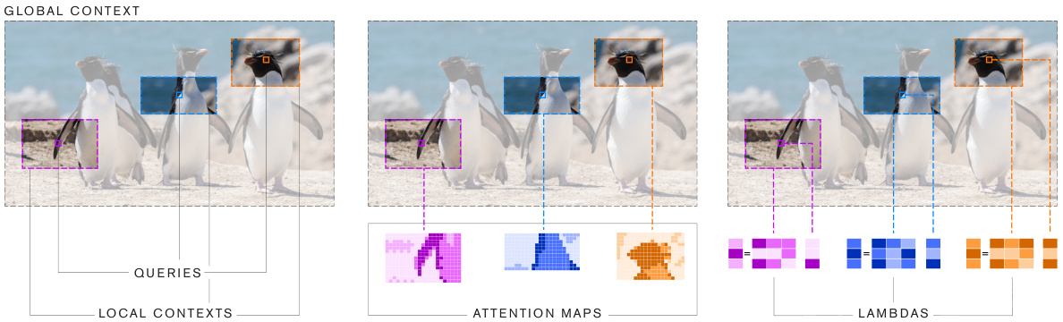
Figure 1: Comparison between self-attention and lambda layers. (Left) An example of 3 queries and their local contexts within a global context. (Middle) Self-attention associates each query with an attention distribution over its context. (Right) The lambda layer transforms each context into a linear function lambda that is applied to the corresponding query.

图 1: 自注意力机制与lambda层的对比。(左) 3个查询及其在全局上下文中的局部上下文示例。(中) 自注意力机制为每个查询生成一个基于其上下文的注意力分布。(右) lambda层将每个上下文转换为线性函数lambda并应用于对应查询。

Lambda layers are versatile and can be implemented to model both content-based and position-based interactions in global, local or masked contexts. The resulting neural networks, Lambda Networks, are computationally efficient, model long-range dependencies at a small memory cost and can therefore be applied to large structured inputs such as high resolution images.

Lambda层具有多功能性，可用于建模全局、局部或掩码上下文中的基于内容和基于位置的交互。由此产生的神经网络——Lambda网络，计算效率高，能以较小的内存成本建模长程依赖关系，因此可应用于高分辨率图像等大型结构化输入。

We evaluate Lambda Networks on computer vision tasks where works using self-attention are hindered by large memory costs (Wang et al., 2018; Bello et al., 2019), suffer impractical implementations (Rama chandra n et al., 2019), or require vast amounts of data (Do sov it ski y et al., 2020). In our experiments spanning ImageNet classification, COCO object detection and COCO instance segmentation, Lambda Networks significantly outperform their convolutional and attention al counterparts, while being more computationally efficient and faster than the latter. We summarize our contributions:

我们在计算机视觉任务上评估了Lambda Networks，这些任务中基于自注意力(self-attention)的工作常受限于高昂内存开销(Wang等人，2018；Bello等人，2019)、存在实现可行性问题(Ramachandran等人，2019)或需要海量数据(Dosovitskiy等人，2020)。在ImageNet分类、COCO目标检测和COCO实例分割的实验中，Lambda Networks在计算效率与速度均优于卷积和注意力机制方案的同时，取得了显著性能提升。我们的贡献总结如下：

A content-based interaction considers the content of the context but ignores the relation between

the query position and the context (e.g. relative distance between two pixels). A position-based interaction considers the relationbetween the query position and the context position.

基于内容的交互 (content-based interaction) 会考虑上下文内容但忽略查询位置与上下文的关系 (例如两个像素的相对距离) 。基于位置的交互 (position-based interaction) 会考虑查询位置与上下文位置的关系。

Table 1: Definition of content-based vs position-based interactions.

表 1: 基于内容与基于位置的交互定义。

simply replacing the 3x3 convolutions in the bottleneck blocks of the ResNet-50 architecture (He et al., 2016) with lambda layers yields a $+1.5%$ top-1 ImageNet accuracy improvement while reducing parameters by $40%$ .

只需将ResNet-50架构(He et al., 2016)瓶颈块中的3x3卷积替换为lambda层，就能在减少40%参数量的同时，将ImageNet top-1准确率提升1.5%。

2 MODELING LONG-RANGE INTERACTIONS

2 长程交互建模

In this section, we formally define queries, contexts and interactions. We motivate keys as a requirement for capturing interactions between queries and their contexts and show that lambda layers arise as an alternative to attention mechanisms for capturing long-range interactions.

在本节中，我们正式定义查询(query)、上下文(context)和交互(interaction)。我们将键(key)作为捕捉查询与其上下文之间交互的必要条件，并展示lambda层可作为注意力机制的替代方案来捕捉长程交互。

Notation. We denote scalars, vectors and tensors using lower-case, bold lower-case and bold upper-case letters, e.g., $n,x$ and $\boldsymbol{X}$ . We denote $|n|$ the cardinality of a set whose elements are indexed by $n$ . We denote ${\boldsymbol{x}}_ {n}$ the $n$ -th row of $\boldsymbol{X}$ . We denote $x_{i j}$ the $|i j|$ elements of $\boldsymbol{X}$ . When possible, we adopt the terminology of self-attention to ease readability and highlight differences.

符号表示。我们用小写字母、粗体小写字母和粗体大写字母分别表示标量、向量和张量，例如 $n,x$ 和 $\boldsymbol{X}$。用 $|n|$ 表示由 $n$ 索引的集合的基数。用 ${\boldsymbol{x}}_ {n}$ 表示 $\boldsymbol{X}$ 的第 $n$ 行。用 $x_{i j}$ 表示 $\boldsymbol{X}$ 的 $|i j|$ 元素。在可能的情况下，我们采用自注意力 (self-attention) 的术语以提高可读性并突出差异。

Defining queries and contexts. Let ${\mathcal{Q}}={(\pmb{q}_ {n},n)}$ and ${\mathcal{C}}={(c_{m},m)}$ denote structured collections of vectors, respectively referred to as the queries and the context. Each query $(\pmb q_{n},n)$ is characterized by its content $\pmb q_{n}\in\mathbb{R}^{|k|}$ and position $n$ . Similarly, each context element $(\pmb{c}_ {m},m)$ is characterized by its content $c_{m}$ and its position $m$ in the context. The $(n,m)$ pair may refer to any pairwise relation between structured elements, e.g. relative distances between pixels or edges between nodes in a graph.

定义查询与上下文。设 ${\mathcal{Q}}={(\pmb{q}_ {n},n)}$ 和 ${\mathcal{C}}={(c_{m},m)}$ 分别表示结构化向量集合，称为查询和上下文。每个查询 $(\pmb q_{n},n)$ 由其内容 $\pmb q_{n}\in\mathbb{R}^{|k|}$ 和位置 $n$ 表征。类似地，每个上下文元素 $(\pmb{c}_ {m},m)$ 由其内容 $c_{m}$ 及其在上下文中的位置 $m$ 表征。$(n,m)$ 对可指代结构化元素间的任意成对关系，例如像素间的相对距离或图中节点间的边。

Defining interactions. We consider the general problem of mapping a query $(\pmb q_{n},n)$ to an output vector $\pmb{y}_ {n}\in\mathbb{R}^{|v|}$ given the context $\mathcal{C}$ with a function $F:((\pmb{q}_ {n},n),\mathcal{C})\mapsto\pmb{y}_ {n}$ . Such a function may act as a layer in a neural network when processing structured inputs. We refer to $(\pmb{q}_ {n},\pmb{c}_ {m})$ interactions as content-based and $(\pmb q_{n},(n,m))$ interactions as position-based. We note that while absolute positional information is sometimes directly added to the query (or context element) content3, we consider this type of interaction to be content-based as it ignores the relation $(n,m)$ between the query and context element positions.

定义交互。我们考虑将查询 $( \pmb q_{n},n )$ 映射到输出向量 $\pmb{y}_ {n}\in\mathbb{R}^{|v|}$ 的通用问题，给定上下文 $\mathcal{C}$ 和函数 $F:((\pmb{q}_ {n},n),\mathcal{C})\mapsto\pmb{y}_ {n}$。在处理结构化输入时，此类函数可作为神经网络的层。我们将 $(\pmb{q}_ {n},\pmb{c}_ {m})$ 交互称为基于内容的交互，而 $(\pmb q_{n},(n,m))$ 交互称为基于位置的交互。需要注意的是，虽然绝对位置信息有时会直接添加到查询（或上下文元素）内容中 [3]，但我们认为此类交互仍属于基于内容，因为它忽略了查询与上下文元素位置之间的关系 $(n,m)$。

Introducing keys to capture long-range interactions. In the context of deep learning, we prioritize fast batched linear operations and use dot-product operations as our interactions. This motivates introducing vectors that can interact with the queries via a dot-product operation and therefore have the same dimension as the queries. In particular, content-based interactions $\left({{q}_ {n}},{{c}_ {m}}\right)$ require a $|k|$ -dimensional vector that depends on $c_{m}$ , commonly referred to as the key $k_{m}$ . Conversely, position-based interactions $(\pmb q_{n},(n,m))$ require a relative position embedding $e_{n m}\in\mathbb{R}^{|k|}$ (Shaw et al., 2018). As the query/key depth $|k|$ and context spatial dimension $|m|$ are not in the output $\pmb{y}_{n}\in\mathbb{R}^{|v|}$ , these dimensions need to be contracted as part of the layer computations. Every layer capturing long-range interactions can therefore be characterized based on whether it contracts the query depth or the context positions first.

引入键(key)以捕捉长程交互。在深度学习背景下，我们优先考虑快速批处理线性运算，并采用点积运算作为交互方式。这促使我们引入能与查询(query)通过点积交互的向量，因此其维度需与查询相同。具体而言：

基于内容的交互 $\left({{q}_ {n}},{{c}_ {m}}\right)$ 需要一个依赖 $c_{m}$ 的 $|k|$ 维向量，通常称为键 $k_{m}$；
基于位置的交互 $(\pmb q_{n},(n,m))$ 则需要相对位置嵌入 $e_{n m}\in\mathbb{R}^{|k|}$ (Shaw et al., 2018)。

由于查询/键深度 $|k|$ 和上下文空间维度 $|m|$ 不会出现在输出 $\pmb{y}_{n}\in\mathbb{R}^{|v|}$ 中，这些维度需作为层计算的一部分进行收缩。因此，每个捕捉长程交互的层可根据其优先收缩查询深度还是上下文位置来表征。

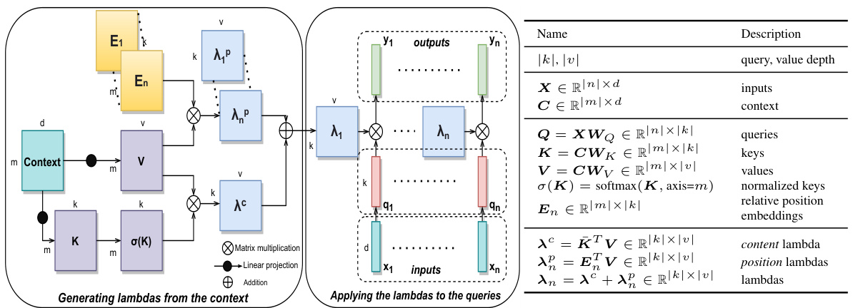
Figure 2: Computational graph of the lambda layer. Contextual information for query position $n$ is summarized into a lambda $\lambda_{n}\in\mathbb{R}^{|k|\times|v|}$ . Applying the lambda dynamically distributes contextual features to produce the output as $\pmb{y}_ {n}=\dot{\lambda}_ {n}^{T}\dot{\pmb{q}_{n}}$ . This process captures content-based and position-based interactions without producing attention maps.

图 2: Lambda层的计算图。查询位置$n$的上下文信息被汇总为一个lambda$\lambda_{n}\in\mathbb{R}^{|k|\times|v|}$。应用该lambda动态分配上下文特征以生成输出$\pmb{y}_ {n}=\dot{\lambda}_ {n}^{T}\dot{\pmb{q}_{n}}$。此过程无需生成注意力图即可捕获基于内容和基于位置的交互。

Attention al interactions. Contracting the query depth first creates a similarity kernel (the attention map) between the query and context elements and is known as the attention operation. As the number of context positions $|m|$ grows larger and the input and output dimensions $|k|$ and $|v|$ remain fixed, one may hypothesize that computing attention maps become wasteful, given that the layer output is a vector of comparatively small dimension $|v|\ll|m|$ .

注意力交互。首先收缩查询深度会在查询和上下文元素之间创建一个相似性核（即注意力图），这一过程被称为注意力操作。随着上下文位置数量 $|m|$ 增大，而输入输出维度 $|k|$ 和 $|v|$ 保持不变，考虑到该层输出是维度相对较小的向量 $|v|\ll|m|$，可以推测计算注意力图会变得低效。

Lambda interactions. Instead, it may be more efficient to simply map each query to its output as ${\pmb y}_ {n}=F(({\pmb q}_ {n},n),{\mathcal{C}})=\lambda({\mathcal{C}},n)({\pmb q}_ {n})$ for some linear function $\dot{\lambda(\mathcal{C},n)}:\mathbb{R}^{|k|}\stackrel{..}{\rightarrow}\mathbb{R}^{|v|}$ . In this scenario, the context is aggregated into a fixed-size linear function $\lambda_{n}=\lambda({\mathcal{C}},n)$ . Each $\lambda_{n}$ acts as a small linear function4 that exists independently of the context (once computed) and is discarded after being applied to its associated query $q_{n}$ .

Lambda交互。相反，更高效的做法可能是直接将每个查询映射到其输出，即 ${\pmb y}_ {n}=F(({\pmb q}_ {n},n),{\mathcal{C}})=\lambda({\mathcal{C}},n)({\pmb q}_ {n})$ ，其中 $\dot{\lambda(\mathcal{C},n)}:\mathbb{R}^{|k|}\stackrel{..}{\rightarrow}\mathbb{R}^{|v|}$ 为某个线性函数。在此场景中，上下文被聚合为一个固定大小的线性函数 $\lambda_{n}=\lambda({\mathcal{C}},n)$ 。每个 $\lambda_{n}$ 作为独立于上下文（一旦计算完成）存在的小型线性函数4，并在应用于其关联查询 $q_{n}$ 后被丢弃。

3 LAMBDA LAYERS

3 LAMBDA 层

3.1 LAMBDA LAYER: TRANSFORMING CONTEXTS INTO LINEAR FUNCTIONS.

3.1 LAMBDA 层：将上下文转换为线性函数

A lambda layer takes the inputs $X\in\mathbb{R}^{|n|\times d_{i n}}$ and the context $C\in\mathbb{R}^{|m|\times d_{c}}$ as input and generates linear function lambdas that are then applied to the queries, yielding outputs $\bar{Y}\in\mathbb{R}^{|n|\times d_{o u t}}$ . Without loss of generality, we assume $d_{i n}=d_{c}=d_{o u t}=d$ . As is the case with $s e l f$ -attention, we we may have $C=X$ . In the rest of this paper, we focus on a specific instance of a lambda layer and show that it captures long-range content and position-based interactions without materializing attention maps. Figure 2 presents the computational graph of the lambda layer.

Lambda层以输入 $X\in\mathbb{R}^{|n|\times d_{i n}}$ 和上下文 $C\in\mathbb{R}^{|m|\times d_{c}}$ 作为输入，生成线性函数lambda，随后将其应用于查询(query)以产生输出 $\bar{Y}\in\mathbb{R}^{|n|\times d_{o u t}}$ 。在不失一般性的前提下，我们假设 $d_{i n}=d_{c}=d_{o u t}=d$ 。与自注意力(self-attention)机制类似，可能存在 $C=X$ 的情况。本文后续将聚焦于lambda层的一个具体实例，展示其无需显式构建注意力图即可捕获长距离内容与基于位置的交互。图2展示了lambda层的计算图。

We first describe the lambda layer when applied to a single query $(\pmb q_{n},n)$ .

我们首先描述应用于单个查询 $(\pmb q_{n},n)$ 的 lambda 层。

Generating the contextual lambda function. We wish to generate a linear function $\mathbb{R}^{|k|}\rightarrow\mathbb{R}^{|v|}$ , i.e. a matrix $\lambda_{n}\in\mathbb{R}^{|k|\times|v|}$ . The lambda layer first computes keys $\kappa$ and values $V$ by linearly projecting the context, and keys are normalized across context positions via a softmax operation yielding normalized keys $\bar{\kappa}$ . The $\lambda_{n}$ matrix is obtained by using the normalized keys $\bar{\kappa}$ and position embeddings $E_{n}$ to aggregate the values $V$ as

生成上下文lambda函数。我们希望生成一个线性函数$\mathbb{R}^{|k|}\rightarrow\mathbb{R}^{|v|}$，即一个矩阵$\lambda_{n}\in\mathbb{R}^{|k|\times|v|}$。lambda层首先通过对上下文进行线性投影计算键$\kappa$和值$V$，并通过softmax操作对上下文位置上的键进行归一化，得到归一化键$\bar{\kappa}$。矩阵$\lambda_{n}$是通过使用归一化键$\bar{\kappa}$和位置嵌入$E_{n}$来聚合值$V$得到的。

$$
\lambda_{n}=\sum_{m}({\bar{k}}_ {m}+e_{n m}){\pmb v}_ {m}^{T}=\underbrace{{\bar{\bf K}}^{T}{\pmb V}}_ {\mathrm{contentlambda}}+\underbrace{\pmb{E}_ {n}^{T}{\pmb V}}_{\mathrm{positionlambda}}\in\mathbb{R}^{|k|\times|v|}
$$

where we also define the content lambda λc and position lambda λpn.

我们还定义了内容lambda λc和位置lambda λpn。

Applying lambda to its query. The query $q_{n}\in\mathbb{R}^{|k|}$ is obtained from the input ${\boldsymbol{x}}_{n}$ via a learned linear projection and the output of the lambda layer is obtained as

将lambda应用于其查询。查询$q_{n}\in\mathbb{R}^{|k|}$通过学习的线性投影从输入${\boldsymbol{x}}_{n}$获得，lambda层的输出计算如下

$$
\pmb{y}_ {n}=\pmb{\lambda}_ {n}^{T}\pmb{q}_ {n}=(\pmb{\lambda}^{c}+\pmb{\lambda}_ {n}^{p})^{T}\pmb{q}_{n}\in\mathbb{R}^{|v|}.
$$

Interpretation of lambda layers. The columns of the $\lambda_{n}\in\mathbb{R}^{|k|\times|v|}$ matrix can be viewed as a fixed-size set of $|k|$ contextual features. These contextual features are aggregated based on the context’s content (content-based interactions) and structure (position-based interactions). Applying the lambda then dynamically distributes these contextual features based on the query to produce the output as $\begin{array}{r}{{\pmb y}_ {n}=\sum_{k}q_{n k}{\pmb\lambda}_{n k}}\end{array}$ . This process captures content and position-based interactions without producing atten tion maps.

Lambda层的解释。矩阵$\lambda_{n}\in\mathbb{R}^{|k|\times|v|}$的列可视为一组固定大小的$|k|$个上下文特征。这些上下文特征基于上下文内容（基于内容的交互）和结构（基于位置的交互）进行聚合。随后应用lambda运算，根据查询(query)动态分配这些上下文特征，生成输出$\begin{array}{r}{{\pmb y}_ {n}=\sum_{k}q_{n k}{\pmb\lambda}_{n k}}\end{array}$。该过程在不生成注意力图(attention maps)的情况下，捕获了基于内容和位置的交互。

Normalization. One may modify Equations 1 and 2 to include non-linear i ties or normalization operations. Our experiments indicate that applying batch normalization (Ioffe & Szegedy, 2015) after computing the queries and the values is helpful.

归一化。可以对公式1和公式2进行修改，加入非线性或归一化操作。实验表明，在计算查询(query)和值(value)后应用批量归一化(batch normalization) [20] 是有效的。

3.2 A MULTI-QUERY FORMULATION TO REDUCE COMPLEXITY.

3.2 降低复杂度的多查询 (Multi-Query) 方案

Complexity analysis. For a batch of $|b|$ examples, each containing $|n|$ inputs, the number of arithmetic operations and memory footprint required to apply our lambda layer are respectively $\Theta(b n m k v)$ and $\Theta(k n m+b n k v)$ . We still have a quadratic memory footprint with respect to the input length due to the $e_{n m}$ relative position embeddings. However this quadratic term does not scale with the batch size as is the case with the attention operation which produces per-example attention maps. In practice, the hyper parameter $|k|$ is set to a small value (such as $|k|{=}16)$ and we can process large batches of large inputs in cases where attention cannot (see Table 4). Additionally, position embeddings can be shared across lambda layers to keep their $\Theta(k n m)$ memory footprint constant - whereas the memory footprint of attention maps scales with the number of layers5.

复杂度分析。对于包含 $|b|$ 个样例的批次，每个样例有 $|n|$ 个输入，应用我们的 lambda 层所需的算术运算次数和内存占用分别为 $\Theta(b n m k v)$ 和 $\Theta(k n m+b n k v)$。由于 $e_{n m}$ 相对位置嵌入的存在，我们仍然面临与输入长度平方相关的内存占用。但这个平方项不会像注意力操作那样随批次大小而扩展，后者会为每个样例生成注意力图。实践中，超参数 $|k|$ 被设置为较小值（例如 $|k|{=}16)$，这使得我们能够处理注意力机制无法应对的大批量长输入情况（见表 4）。此外，位置嵌入可以在多个 lambda 层间共享，从而保持其 $\Theta(k n m)$ 的内存占用恒定——而注意力图的内存占用会随网络层数增加而增长[5]。

Multi-query lambda layers reduce time and space complexities. Recall that the lambda layer maps inputs $\pmb{x}_ {n}\in\mathbb{R}^{d}$ to outputs $\pmb{y}_ {n}\in\mathbb{R}^{d}$ . As presented in Equation 2, this implies that $|v|{=}d$ . Small values of $|v|$ may therefore act as a bottleneck on the feature vector ${\mathbf{}}_ {{\mathbf{}}}{\mathbf{}}_ {{\mathbf{}}}{\mathbf{}}_ {{\mathbf{}}}{\mathbf{}}_ {{\mathbf{}}}{\mathbf{}}_ {{\mathbf{}}}{\mathbf{}}_ {{\mathbf{}}}{\mathbf{}}_ {{\mathbf{}}}{\mathbf{}}_ {{\mathbf{}}}{\mathbf{}}_ {{\mathbf{}}}{\mathbf{}}_ {{\mathbf{}}}{\mathbf{}}_{{\mathbf{}}}$ but larger output dimensions $|v|$ can incur an excessively large computational cost given our $\Theta(b n m k v)$ and $\Theta(k n m+b n k v)$ time and space complexities.

多查询lambda层降低了时间和空间复杂度。回顾lambda层将输入$\pmb{x}_ {n}\in\mathbb{R}^{d}$映射到输出$\pmb{y}_ {n}\in\mathbb{R}^{d}$。如公式2所示，这意味着$|v|{=}d$。较小的$|v|$值可能成为特征向量${\mathbf{}}_ {{\mathbf{}}}{\mathbf{}}_ {{\mathbf{}}}{\mathbf{}}_ {{\mathbf{}}}{\mathbf{}}_ {{\mathbf{}}}{\mathbf{}}_ {{\mathbf{}}}{\mathbf{}}_ {{\mathbf{}}}{\mathbf{}}_ {{\mathbf{}}}{\mathbf{}}_ {{\mathbf{}}}{\mathbf{}}_ {{\mathbf{}}}{\mathbf{}}_{{\mathbf{}}}$的瓶颈，而较大的输出维度$|v|$在$\Theta(b n m k v)$和$\Theta(k n m+b n k v)$的时间与空间复杂度下会产生过高的计算成本。

We propose to decouple the time and space complexities of our lambda layer from the output dimension $d$ . Rather than imposing $|v|{=}\mathrm{d}$ , we create $|h|$ queries ${\pmb q_{n}^{h}}$ , apply the same lambda $\lambda_{n}$ to each query $\pmb q_{n}^{h}$ , and concatenate the outputs as ${\pmb y}_ {n}=\mathrm{concat}({\pmb\lambda}_ {n}{\pmb q}_ {n}^{1},\cdot\cdot\cdot,{\pmb\lambda}_ {n}{\pmb q}_ {n}^{|h|})$ . We now have $|v|{=}d/|h|$ , which reduces complexity by a factor of $|h|$ . The number of heads $|h|$ controls the size of the lambdas $\lambda_{n}\in\mathbb{R}^{|k|\times|d|/|h|}$ relative to the total size of the queries $\pmb q_{n}\in\mathbb{R}^{|h k|}$ .

我们提出将lambda层的时间和空间复杂度与输出维度$d$解耦。不再强制要求$|v|{=}\mathrm{d}$，而是创建$|h|$个查询${\pmb q_{n}^{h}}$，对每个查询$\pmb q_{n}^{h}$应用相同的lambda$\lambda_{n}$，并将输出拼接为${\pmb y}_ {n}=\mathrm{concat}({\pmb\lambda}_ {n}{\pmb q}_ {n}^{1},\cdot\cdot\cdot,{\pmb\lambda}_ {n}{\pmb q}_ {n}^{|h|})$。此时$|v|{=}d/|h|$，复杂度降低了$|h|$倍。头数$|h|$控制lambda$\lambda_{n}\in\mathbb{R}^{|k|\times|d|/|h|}$相对于查询$\pmb q_{n}\in\mathbb{R}^{|h k|}$总大小的比例。

def lambda_layer(queries，1 """Multi-query #b:batch，n: #k: query/key # h: number of content_lambda = einsum(softmax(keys)，values，'bmk,bmv->bkv')

We refer to this operation as a multi-query lambda layer and present an implementation using einsum6 in Figure 3. The lambda layer is robust to $|k|$ and $|h|$ hyper parameter choices (see Appendix D.1), which enables flexibility in controlling its complexity. We use $\vert h\vert{=}4$ in most experiments.

我们将这一操作称为多查询lambda层，并在图3中展示了使用einsum6的实现方式。该lambda层对超参数$|k|$和$|h|$的选择具有鲁棒性（见附录D.1），从而能够灵活控制其复杂度。在大多数实验中，我们使用$\vert h\vert{=}4$。

We note that while this resembles the multi-head or multi-query (Shazeer, 2019)7 attention formulation, the motivation is different. Using multiple queries in the attention operation increases represent at ional power and complexity. In contrast, using multiple queries in the lambda layer decreases complexity and representational power (ignoring the additional queries).

我们注意到，虽然这与多头或多查询 (Shazeer, 2019) [7] 注意力公式相似，但动机不同。在注意力操作中使用多个查询会增加表示能力和复杂性。相反，在 lambda 层中使用多个查询会降低复杂性和表示能力 (忽略额外的查询)。

Extending the multi-query formulation to linear attention. Finally, we point that our analysis extends to linear attention which can be viewed as a content-only lambda layer (see Appendix C.3 for a detailed discussion). We anticipate that the multi-query formulation can also bring computational benefits to linear attention mechanisms.

将多查询(multi-query)公式扩展到线性注意力机制。最后需要指出，我们的分析同样适用于线性注意力机制——这种机制可被视为仅含内容的lambda层(详见附录C.3)。我们预计多查询公式也能为线性注意力机制带来计算优势。

3.3 MAKING LAMBDA LAYERS TRANSLATION E QUI VARIANT.

3.3 实现Lambda层翻译等效变体

Using relative position embeddings $e_{n m}$ enables making explicit assumptions about the structure of the context. In particular, translation e qui variance (i.e. the property that shifting the inputs results in an equivalent shift of the outputs) is a strong inductive bias in many learning scenarios. We obtain translation e qui variance in position interactions by ensuring that the position embeddings satisfy $e_{n m}=e_{t(n)t(m)}$ for any translation $t$ . In practice, we define a tensor of relative position embeddings $\pmb{R}\in\mathbb{R}^{|r|\times|k|}$ , where $r$ indexes the possible relative positions for all $(n,m)$ pairs, and reindex8 it into $\pmb{{\cal E}}\in\mathbb{R}^{|n|\times|m|\times|k|}$ such that $e_{n m}=r_{r(n,m)}$ .

使用相对位置嵌入 $e_{n m}$ 能够显式建模上下文的结构假设。其中，平移等变性 (即输入偏移导致输出等效偏移的特性) 是许多学习场景中的强归纳偏置。我们通过确保位置嵌入满足 $e_{n m}=e_{t(n)t(m)}$（对于任意平移 $t$）来实现位置交互的平移等变性。实践中，我们定义相对位置嵌入张量 $\pmb{R}\in\mathbb{R}^{|r|\times|k|}$（其中 $r$ 索引所有 $(n,m)$ 对的可能相对位置），并将其重新索引为 $\pmb{{\cal E}}\in\mathbb{R}^{|n|\times|m|\times|k|}$ 使得 $e_{n m}=r_{r(n,m)}$。

3.4 LAMBDA CONVOLUTION: MODELING LONGER RANGE INTERACTIONS IN LOCAL CONTEXTS.

3.4 LAMBDA卷积：在局部上下文中建模长程交互

Despite the benefits of long-range interactions, locality remains a strong inductive bias in many tasks. Using global contexts may prove noisy or computationally excessive. It may therefore be useful to restrict the scope of position interactions to a local neighborhood around the query position $n$ as is the case for local self-attention and convolutions. This can be done by zeroing out the relative embeddings for context positions $m$ outside of the desired scope. However, this strategy remains costly for large values of $|m|$ since the computations still occur - they are only being zeroed out.

尽管长程交互具有优势，但在许多任务中局部性仍是强归纳偏置。使用全局上下文可能引入噪声或导致计算冗余。因此，将位置交互范围限制在查询位置 $n$ 的局部邻域内可能更为有效，如局部自注意力 (local self-attention) 和卷积操作所示。这可通过将超出目标范围的上下文位置 $m$ 的相对嵌入置零来实现。然而，当 $|m|$ 值较大时，该策略仍存在较高计算成本——因为运算依然执行，只是结果被置零。

Lambda convolution In the case where the context is arranged in a multidimensional grid, we can equivalently compute positional lambdas from local contexts by using a regular convolution.

Lambda卷积
当上下文排列为多维网格时，我们可以通过常规卷积从局部上下文中等价地计算位置lambda。

Table 2: Alternatives for capturing long-range interactions. The lambda layer captures content and position-based interactions at a reduced memory cost compared to relative attention (Shaw et al., 2018; Bello et al., 2019). Using a multi-query lambda layer reduces complexities by a factor of $|h|$ . Additionally, position-based interactions can be restricted to a local scope by using the lambda convolution which has linear complexity. $b$ : batch size, $h$ : number of heads/queries, $n$ : input length, $m$ : context length, $r$ : local scope size, $k$ : query/key depth, $d$ : dimension output.

Operation	Head configuration	Interactions	Time complexity	Space complexity
Attention Relativeattention	multi-head multi-head	content-only content & position	(bnm(hk + d)) (bnm(hk + d))	O（bhnm bhnm
Lambdalayer Lambdaconvolution	multi-head multi-query multi-query	content-only content&position content & position	O(bnkd) (bnmkd/h) (bnrkd/h)	O（bkd O(knm+bnkd/h) (kr +bnkd/h)

表 2: 捕捉长距离交互的替代方案。与相对注意力 (Shaw et al., 2018; Bello et al., 2019) 相比，lambda层以更低的内存成本捕捉基于内容和位置的交互。使用多查询lambda层可将复杂度降低 $|h|$ 倍。此外，通过使用具有线性复杂度的lambda卷积，可以将基于位置的交互限制在局部范围内。$b$: 批大小, $h$: 头数/查询数, $n$: 输入长度, $m$: 上下文长度, $r$: 局部范围大小, $k$: 查询/键深度, $d$: 输出维度。

操作	头配置	交互	时间复杂度	空间复杂度
注意力相对注意力	多头多头	仅内容内容 & 位置	(bnm(hk + d)) (bnm(hk + d))	O(bhnm bhnm)
Lambda层 Lambda卷积	多头多查询多查询	仅内容内容&位置内容 & 位置	O(bnkd) (bnmkd/h) (bnrkd/h)	O(bkd) O(knm+bnkd/h) (kr +bnkd/h)

We term this operation the lambda convolution. A n-dimensional lambda convolution can be implemented using an n-d depthwise convolution with channel multiplier or (n+1)-d convolution that treats the $v$ dimension in $V$ as an extra spatial dimension. We present both implementations in Appendix B.1.

我们将这一操作称为lambda卷积。n维lambda卷积可以通过使用带有通道乘数的n维深度卷积或将$V$中的$v$维度视为额外空间维度的(n+1)维卷积来实现。我们在附录B.1中提供了这两种实现方案。

As the computations are now restricted to a local scope, the lambda convolution obtains linear time and memory complexities with respect to the input length9. The lambda convolution is readily usable with additional functionalities such as dilation and striding and enjoys optimized implementations on specialized hardware accelerators (Nickolls & Dally, 2010; Jouppi et al., 2017). This is in stark contrast to implementations of local self-attention that require materializing feature patches of overlapping query and context blocks (Parmar et al., 2018; Rama chandra n et al., 2019), increasing memory consumption and latency (see Table 4).

由于计算现在被限制在局部范围内，Lambda卷积在输入长度上实现了线性的时间和内存复杂度[9]。Lambda卷积可直接配合膨胀(dilation)和步长(striding)等附加功能使用，并能在专用硬件加速器上获得优化实现 (Nickolls & Dally, 2010; Jouppi et al., 2017)。这与局部自注意力(local self-attention)的实现形成鲜明对比——后者需要实例化重叠查询块和上下文块的特征补丁 (Parmar et al., 2018; Ramachandran et al., 2019)，从而增加内存消耗和延迟(见表4)。

4 相关工作

Table 2 reviews alternatives for capturing long-range interactions and contrasts them with the proposed multi-query lambda layer. We discuss related works in details in the Appendix C.

表 2: 回顾了捕捉长程交互的替代方案，并与提出的多查询 lambda 层进行对比。附录 C 详细讨论了相关工作。

Channel and linear attention The lambda abstraction, i.e. transforming available contexts into linear functions that are applied to queries, is quite general and therefore encompasses many previous works. Closest to our work are channel and linear attention mechanisms (Hu et al., 2018c; Katha ro poul os et al., 2020; Cho roman ski et al., 2020). Such mechanisms also capture long-range interactions without materializing attention maps and can be viewed as specific instances of a contentonly lambda layer. Lambda layers formalize and extend such approaches to consider both contentbased and position-based interactions, enabling their use as a stand-alone layer on highly structured data such as images. Rather than attempting to closely approximate an attention kernel as is the case with linear attention, we focus on the efficient design of contextual lambda functions and repurpose a multi-query formulation (Shazeer, 2019) to further reduce computational costs.

通道与线性注意力
Lambda抽象(即将可用上下文转化为应用于查询的线性函数)具有高度通用性，因此涵盖了许多先前工作。与我们研究最接近的是通道注意力和线性注意力机制(Hu et al., 2018c; Katharopoulos et al., 2020; Choromanski et al., 2020)。这些机制同样无需显式构建注意力图就能捕获长程交互，可视为纯内容型lambda层的特定实例。Lambda层通过形式化扩展这些方法，同时考虑基于内容和基于位置的交互，使其能作为独立层处理高度结构化数据(如图像)。不同于线性注意力试图紧密逼近注意力核的做法，我们专注于上下文lambda函数的高效设计，并复用多查询框架(Shazeer, 2019)以进一步降低计算成本。

Self-attention in the visual domain In contrast to natural language processing tasks where it is now the de-facto standard, self-attention has enjoyed steady but slower adoption in the visual domain (Wang et al., 2018; Bello et al., 2019; Rama chandra n et al., 2019; Carion et al., 2020). Concurrently to this work, Do sov it ski y et al. (2020) achieve a strong $88.6%$ accuracy on ImageNet by pre-training a Transformer on sequences of image patches on a large-scale dataset of 300M images.

视觉领域的自注意力机制
与自然语言处理任务中自注意力已成为事实标准不同，视觉领域对自注意力机制的采用虽稳步推进但相对缓慢 (Wang et al., 2018; Bello et al., 2019; Ramachandran et al., 2019; Carion et al., 2020)。在本研究同期，Dosovitskiy等人 (2020) 通过在3亿张图像的大规模数据集上对图像块序列预训练Transformer，在ImageNet上实现了88.6%的高准确率。

5 EXPERIMENTS

5 实验

In subsequent experiments, we evaluate lambda layers on standard computer vision benchmarks: ImageNet classification (Deng et al., 2009), COCO object detection and instance segmentation (Lin et al., 2014). The visual domain is well-suited to showcase the flexibility of lambda layers since (1) the memory footprint of self-attention becomes problematic for high-resolution imagery and (2) images are highly structured, making position-based interactions crucial.

在后续实验中，我们在标准计算机视觉基准上评估lambda层：ImageNet分类 (Deng et al., 2009)、COCO目标检测与实例分割 (Lin et al., 2014)。视觉领域非常适合展示lambda层的灵活性，因为：(1) 自注意力(self-attention)的内存占用对高分辨率图像会形成瓶颈；(2) 图像具有高度结构性，使得基于位置的交互至关重要。

Lambda Res Nets We construct Lambda Res Nets by replacing the 3x3 convolutions in the bottleneck blocks of the ResNet architecture (He et al., 2016). When replacing all such convolutions, we simply denote the name of the layer being tested (e.g. conv $^+$ channel attention or lambda layer). We denote Lambda Res Nets the family of hybrid architectures described in Table 18 (Appendix E.1). Unless specified otherwise, all lambda layers use $|k|{=}16$ , $|h|{=}4$ with a scope size of $|m|{=}23\mathrm{x}23$ and are implemented as in Figure 3. Additional experiments and details can be found in the Appendix.

Lambda Res Nets
我们通过替换ResNet架构 (He et al., 2016) 瓶颈块中的3x3卷积来构建Lambda Res Nets。当替换所有此类卷积时，我们仅标注被测试层的名称（例如conv $^+$ 通道注意力或lambda层）。Lambda Res Nets指代表18（附录E.1）中描述的混合架构家族。除非另有说明，所有lambda层均使用 $|k|{=}16$ 、 $|h|{=}4$ ，作用域大小为 $|m|{=}23\mathrm{x}23$ ，其实现如图3所示。更多实验细节详见附录。

5.1 LAMBDA LAYERS OUTPERFORM CONVOLUTIONS AND ATTENTION LAYERS.

5.1 LAMBDA层性能优于卷积层和注意力层

We first consider the standard ResNet-50 architecture with input image size $224\mathrm{x}224$ . In Table 3, we compare the lambda layer against (a) the standard convolution (i.e. the baseline ResNet-50) (b) channel attention (squeeze-and-excitation) and (c) multiple self-attention variants. The lambda layer strongly outperforms all baselines at a fraction of the parameter cost and notably obtains a $+0.8%$ improvement over channel attention.

我们首先考虑输入图像尺寸为 $224\mathrm{x}224$ 的标准 ResNet-50 架构。在表 3 中，我们将 lambda 层与以下方法进行对比：(a) 标准卷积(即基线 ResNet-50)、(b) 通道注意力(squeeze-and-excitation)以及(c) 多种自注意力变体。lambda 层以极少的参数量显著优于所有基线方法，特别是相比通道注意力获得了 $+0.8%$ 的提升。

Table 3: Comparison of the lambda layer and attention mechanisms on ImageNet classification with a ResNet50 architecture. The lambda layer strongly outperforms attention alternatives at a fraction of the parameter cost. All models are trained in mostly similar setups (see Appendix E.2) and we include the reported improvements compared to the convolution baseline in parentheses. See Appendix B.4 for a description of the $|u|$ hyper parameter. † Our implementation.

Layer	Params (M)	top-1
Conv (He et al.,2016)t	25.6	76.9
Conv + channel attention (Hu et al.,2018c)	28.1	77.6 (+0.7)
Conv+linear attention (Chenet al.,2018)	33.0	77.0
Conv + linear attention (Shen et al., 2018)		77.3 (+1.2)
Conv +relative self-attention(Bello et al.,2019)	25.8	77.7 (+1.3)
Local relative self-attention (Ramachandran et al.,2019)	18.0	77.4 (+0.5)
Localrelativeself-attention(Huetal.,2019)	23.3	77.3 (+1.0)
Local relative self-attention (Zhao et al.,2020)	20.5	78.2 (+1.3)
Lambda layer	15.0	78.4 (+1.5)
Lambda layer (\|u\|=4)	16.0	78.9 (+2.0)

表 3: 在ResNet50架构的ImageNet分类任务上，lambda层与注意力机制的对比。lambda层以极少的参数量显著优于各类注意力变体。所有模型均在基本相同的设置下训练（详见附录E.2），括号内为相对卷积基线的改进值。超参数$|u|$的说明见附录B.4。†表示我们的实现。

Layer	Params (M)	top-1
Conv (He et al.,2016)†	25.6	76.9
Conv + channel attention (Hu et al.,2018c)	28.1	77.6 (+0.7)
Conv+linear attention (Chen et al.,2018)	33.0	77.0
Conv + linear attention (Shen et al., 2018)	-	77.3 (+1.2)
Conv +relative self-attention(Bello et al.,2019)	25.8	77.7 (+1.3)
Local relative self-attention (Ramachandran et al.,2019)	18.0	77.4 (+0.5)
Localrelativeself-attention(Hu et al.,2019)	23.3	77.3 (+1.0)
Local relative self-attention (Zhao et al.,2020)	20.5	78.2 (+1.3)
Lambda layer	15.0	78.4 (+1.5)
Lambda layer (	u	=4)

.2 COMPUTATIONAL BENEFITS OF LAMBDA LAYERS OVER SELF-ATTENTIO

2.2 Lambda层相较于自注意力机制的计算优势

In Table 4, we compare lambda layers against self-attention and present through puts, memory complexities and ImageNet accuracies. Our results highlight the weaknesses of self-attention: selfattention cannot model global interactions due to large memory costs, axial self-attention is still memory expensive and local self-attention is prohibitively slow. In contrast, the lambda layer can capture global interactions on high-resolution images and obtains a $+1.0%$ improvement over local self-attention while being almost $3\mathbf{x}$ faster10. Additionally, positional embeddings can be shared across lambda layers to further reduce memory requirements, at a minimal degradation cost. Finally, the lambda convolution has linear memory complexity, which becomes practical for very large images as seen in detection or segmentation. We also find that the lambda layer outperforms local self-attention when controlling for the scope size11 ( $78.1%$ vs $77.4%$ for $|m|{=}7\mathbf{x}7,$ , suggesting that the benefits of the lambda layer go beyond improved speed and s cal ability.

在表4中，我们将lambda层与自注意力机制(self-attention)进行对比，展示了吞吐量、内存复杂度及ImageNet准确率。结果揭示了自注意力的三大缺陷：全局交互建模因内存开销过大而受限，轴向自注意力仍存在高内存消耗，局部自注意力则存在严重速度瓶颈。相比之下，lambda层能在高分辨率图像上捕捉全局交互，较局部自注意力实现$+1.0%$精度提升的同时提速近$3\mathbf{x}$。通过共享位置嵌入，lambda层可进一步降低内存需求且仅带来微小性能损失。其线性内存复杂度特性使其在检测/分割等超大图像任务中极具实用性。控制感受野范围时，lambda层仍优于局部自注意力( $78.1%$ vs $77.4%$ @ $|m|{=}7\mathbf{x}7$ )，这表明其优势不仅体现在速度与可扩展性层面。

Layer	SpaceComplexity	Memory (GB)	Throughput	top-1
Globalself-attention	O(blhn	120	OOM	OOM
Axialself-attention	O（blhn√n）	4.8	960ex/s	77.5
Local self-attention (7x7)	O（blhnm		440ex/s	77.4
Lambdalayer	(lkn²)	1.9	1160ex/s	78.4
Lambda layer (\|k\|=8)	O(lkn²	0.95	1640ex/s	77.9
Lambda layer (shared embeddings)	O(kn 2	0.63	1210ex/s	78.0
Lambda convolution (7x7)	O(lknm)		1100ex/s	78.1

层	空间复杂度	内存 (GB)	吞吐量	top-1
全局自注意力 (Global self-attention)	O(blhn	120	OOM	OOM
轴向自注意力 (Axial self-attention)	O(blhn√n)	4.8	960ex/s	77.5
局部自注意力 (7x7)	O(blhnm	-	440ex/s	77.4
Lambda层	O(lkn²)	1.9	1160ex/s	78.4
Lambda层 (	k	=8)	O(lkn²	0.95
Lambda层 (共享嵌入)	O(kn²	0.63	1210ex/s	78.0
Lambda卷积 (7x7)	O(lknm)	-	1100ex/s	78.1

Table 4: The lambda layer reaches higher ImageNet accuracies while being faster and more memory-efficient than self-attention alternatives. Memory is reported assuming full precision for a batch of 128 inputs using default hyper parameters. The memory cost for storing the lambdas matches the memory cost of activation s in the rest of the network and is therefore ignored. b: batch size, $h$ : number of heads/queries, $n$ : input length, $m$ : context length, $k$ : query/key depth, l: number of layers.

表 4: Lambda层在达到更高ImageNet准确率的同时，比自注意力替代方案速度更快且内存效率更高。内存数据基于使用默认超参数、128输入批次的全精度计算得出。存储lambda的内存成本与网络中其余部分的激活内存成本相当，因此忽略不计。b: 批次大小, $h$: 头数/查询数, $n$: 输入长度, $m$: 上下文长度, $k$: 查询/键深度, l: 层数。

5.3 HYBRIDS IMPROVE THE SPEED-ACCURACY TRADEOFF OF IMAGE CLASSIFICATION.

5.3 混合模型提升图像分类的速度-准确率权衡

Studying hybrid architectures. In spite of the memory savings compared to self-attention, capturing global contexts with the lambda layer still incurs a quadratic time complexity (Table 2), which remains costly at high resolution. Additionally, one may hypothesize that global contexts are most beneficial once features contain semantic information, i.e. after having been processed by a few operations, in which case using global contexts in the early layers would be wasteful. In the Appendix 5.3, we study hybrid designs that use standard convolutions to capture local contexts and lambda layers to capture global contexts. We find that such convolution-lambda hybrids have increased representational power at a negligible decrease in throughput compared to their purely convolutional counterparts.

研究混合架构。尽管与自注意力(self-attention)相比节省了内存，但使用lambda层捕获全局上下文仍会产生二次时间复杂度(表2)，在高分辨率下成本依然高昂。此外，可以假设全局上下文最有利于包含语义信息的特征，即经过若干操作处理后，在这种情况下早期层使用全局上下文将是浪费的。在附录5.3中，我们研究了使用标准卷积捕获局部上下文和lambda层捕获全局上下文的混合设计。研究发现，与纯卷积架构相比，这种卷积-lambda混合架构在吞吐量几乎不降低的情况下提高了表征能力。

Lambda Res Nets significantly improve the speed-accuracy tradeoff of ImageNet classification. We design a family of hybrid Lambda Res Nets across scales based on our study of hybrid architectures and the scaling/training strategies from Bello et al. (2021) (see Section E.1). Figure 4 presents the speed-accuracy Pareto curve of Lambda Res Nets compared to Efficient Nets (Tan & Le, 2019) on TPUv3 hardware. In order to isolate the benefits of lambda layers, we additionally compare against the same architectures when replacing lambda layers by (1) standard 3x3 convolutions (denoted ResNet-RS wo/ SE) and (2) 3x3 convolutions with squeeze-and-excitation (denoted ResNet-RS w/ SE). All architectures are trained for 350 epochs using the same regular iz ation methods and evaluated at the same resolution they are trained at.

Lambda Res Nets显著提升了ImageNet分类任务中速度与精度的权衡关系。基于对混合架构的研究以及Bello等人(2021)提出的扩展/训练策略(参见E.1节)，我们设计了一系列跨尺度的混合Lambda Res Nets变体。图4展示了在TPUv3硬件上，Lambda Res Nets与Efficient Nets(Tan & Le, 2019)的速度-精度帕累托曲线对比。为了单独评估lambda层的优势，我们还对比了两种变体：(1) 用标准3x3卷积(标记为ResNet-RS wo/SE)替换lambda层，(2) 使用带压缩激励模块的3x3卷积(标记为ResNet-RS w/SE)。所有架构均采用相同的正则化方法训练350个epoch，并在训练分辨率下进行评估。

Lambda Res Nets outperform the baselines across all scales on the speed-accuracy trade-off. LambdaResNets are $3.2\cdot4.4\mathrm{x}$ faster than Efficient Nets and $1.6\cdot2.3\mathrm{x}$ faster than ResNet-RS when controlling for accuracy, thus significantly improving the speed-accuracy Pareto curve of image classification12. Our largest model, Lambda Res Net-420 trained at image size 320, achieves a strong $84.9%$ top-1 ImageNet accuracy, $0.9%$ over the corresponding architecture with standard $3\mathrm{x}3$ convolutions and $0.65%$ over the corresponding architecture with squeeze-and-excitation.

Lambda Res Nets 在速度-准确率权衡方面全面超越基线模型。在控制准确率的情况下，LambdaResNets 比 Efficient Nets 快 $3.2\cdot4.4\mathrm{x}$，比 ResNet-RS 快 $1.6\cdot2.3\mathrm{x}$，显著提升了图像分类任务的速度-准确率帕累托曲线[12]。我们最大的模型 Lambda Res Net-420 在 320 像素图像尺寸下训练，取得了 84.9% 的 ImageNet 最高准确率，比使用标准 $3\mathrm{x}3$ 卷积的对应架构高出 0.9%，比使用压缩激励(squeeze-and-excitation)的对应架构高出 0.65%。

Scaling to larger datasets with pseudo-labels We train Lambda Res Nets in a semi-supervised learning setting using 130M pseudo-labeled images from the JFT dataset, as done for training the Efficient Net-Noisy Student checkpoints (Xie et al., 2020). Table 5 compares the through puts and ImageNet accuracies of a representative set of models with similar accuracies when trained using the JFT dataset. Lambda Res Net-152, trained and evaluated at image size 288, achieves a strong $86.7%$ top-1 ImageNet accuracy while being more parameter-efficient and 9.5x faster than the Efficient NetNoisy Student checkpoint with the same accuracy.

使用伪标签扩展更大数据集
我们采用半监督学习方式训练Lambda Res Nets，使用来自JFT数据集的1.3亿张伪标签图像，该方法与训练Efficient Net-Noisy Student检查点时采用的方式相同(Xie et al., 2020)。表5比较了使用JFT数据集训练时，一组具有相似准确率的代表性模型的吞吐量和ImageNet准确率。在288像素图像尺寸下训练和评估的Lambda Res Net-152，实现了86.7%的ImageNet top-1准确率，同时比具有相同准确率的Efficient Net-Noisy Student检查点参数效率更高、速度快9.5倍。

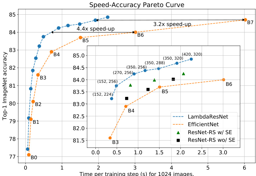
Figure 4: Speed-accuracy comparison between Lambda Res Nets and Efficient Nets. When matching the training and regular iz ation setup of Efficient Nets, Lambda Res Nets are $3.2\textrm{-}4.4\mathrm{X}$ faster than Efficient Nets and $1.6-2.3\mathrm{x}$ faster than ResNet-RS with squeeze-and-excitation. LambdaResNets are annotated with (depth, image size). Our largest Lambda Res Net, Lambda Res Net-420 trained at image size 320, reaches a strong $84.9%$ top-1 accuracy.

图 4: Lambda Res Nets与Efficient Nets的速度-精度对比。当采用与Efficient Nets相同的训练和正则化设置时，Lambda Res Nets比Efficient Nets快$3.2\textrm{-}4.4\mathrm{X}$，比带有squeeze-and-excitation的ResNet-RS快$1.6-2.3\mathrm{x}$。LambdaResNets标注了(深度, 图像尺寸)。我们最大的Lambda Res Net——图像尺寸为320的Lambda Res Net-420，达到了强劲的$84.9%$ top-1准确率。

Table 5: Comparison of models trained on extra data. ViT-L/16 is pre-trained on JFT and finetuned on ImageNet at resolution $384\mathrm{x}384$ , while Efficient Net and Lambda Res Net are co-trained on ImageNet and JFT pseudo-labels. Training and inference throughput is shown for 8 TPUv3 cores.

Architecture	Params s (M)	Train (ex/s)	Infer (ex/s)	ImageNet top-1
LambdaResNet-152	51	1620	6100	86.7
EfficientNet-B7	66	170 (9.5x)	980 (6.2x)	86.7
ViT-L/16	307	180 (9.0x)	640 (9.5x)	87.1

表 5: 基于额外数据训练的模型对比。ViT-L/16 在 JFT 上预训练并在 $384\mathrm{x}384$ 分辨率下对 ImageNet 微调，而 Efficient Net 和 Lambda Res Net 则在 ImageNet 和 JFT 伪标签上联合训练。训练和推理吞吐量基于 8 个 TPUv3 核心展示。

Architecture	Params (M)	Train (ex/s)	Infer (ex/s)	ImageNet top-1
LambdaResNet-152	51	1620	6100	86.7
EfficientNet-B7	66	170 (9.5x)	980 (6.2x)	86.7
ViT-L/16	307	180 (9.0x)	640 (9.5x)	87.1

5.4 OBJECT DETECTION AND INSTANCE SEGMENTATION RESULTS

5.4 目标检测与实例分割结果

In Table 6, we evaluate Lambda Res Nets as a backbone in Mask-RCNN (He et al., 2017) on the COCO object detection and instance segmentation tasks. Using lambda layers yields consistent gains across all object sizes, especially the small objects which are the hardest to locate. This indicates that lambda layers are also competitive for more complex visual tasks that require localization information.

在表6中，我们评估了将Lambda Res Nets作为Mask-RCNN (He et al., 2017) 主干网络在COCO目标检测和实例分割任务中的表现。使用lambda层在所有物体尺寸上都带来了稳定的性能提升，尤其是最难定位的小物体。这表明lambda层对于需要定位信息的更复杂视觉任务同样具有竞争力。

Table 6: COCO object detection and instance segmentation with Mask-RCNN architecture on $\mathbf{1024x1024}$ inputs. Mean Average Precision (AP) for small, medium, large objects $(\mathrm{s}/\mathrm{m}/1)$ . Using lambda layers yields consistent gains across all object sizes, especially small objects.

Backbone	APbb COCO	APbb s/m/l	APmask coco	APmask s/m/l
ResNet-101	48.2	29.9/50.9/64.9	42.6	24.2/45.6/60.0
ResNet-101+SE	48.5	29.9/51.5/65.3	42.8	24.0/46.0/60.2
LambdaResNet-101	49.4	31.7/52.2/65.6	43.5	25.9 / 46.5 / 60.8
ResNet-152	48.9	29.9/51.8/ 66.0	43.2	24.2/46.1/61.2
ResNet-152+SE	49.4	30.0/52.3/66.7	43.5	24.6/46.8/61.8
LambdaResNet-152	50.0	31.8/53.4/67.0	43.9	25.5/47.3/62.0

表 6: 使用Mask-RCNN架构在$\mathbf{1024x1024}$输入尺寸下的COCO目标检测与实例分割结果。小/中/大物体的平均精度均值(AP) $(\mathrm{s}/\mathrm{m}/1)$。采用lambda层在所有物体尺寸上均获得稳定提升，尤其对小物体效果显著。

Backbone	APbb COCO	APbb s/m/l	APmask coco	APmask s/m/l
ResNet-101	48.2	29.9/50.9/64.9	42.6	24.2/45.6/60.0
ResNet-101+SE	48.5	29.9/51.5/65.3	42.8	24.0/46.0/60.2
LambdaResNet-101	49.4	31.7/52.2/65.6	43.5	25.9/46.5/60.8
ResNet-152	48.9	29.9/51.8/66.0	43.2	24.2/46.1/61.2
ResNet-152+SE	49.4	30.0/52.3/66.7	43.5	24.6/46.8/61.8
LambdaResNet-152	50.0	31.8/53.4/67.0	43.9	25.5/47.3/62.0

6 DISCUSSION

6 讨论

How do lambda layers compare to the attention operation? Lambda layers scale favorably compared to self-attention. Vanilla Transformers using self-attention have $\Theta({\bar{b l h n^{2}}})$ memory footprint, whereas Lambda Networks have $\Theta(l k n^{2})$ memory footprint (or $\Theta(k n^{2})$ when sharing positional embeddings across layers). This enables the use of lambda layers at higher-resolution and on larger batch sizes. Additionally, the lambda convolution enjoys a simpler and faster implementation than its local self-attention counterpart. Finally, our ImageNet experiments show that lambda layers outperforms self-attention, demonstrating that the benefits of lambda layers go beyond improved speed and s cal ability.

Lambda层与注意力机制相比如何？
Lambda层在扩展性上优于自注意力机制。使用自注意力的标准Transformer具有$\Theta({\bar{b l h n^{2}}})$的内存占用，而Lambda网络的内存占用为$\Theta(l k n^{2})$（或在层间共享位置嵌入时为$\Theta(k n^{2})$）。这使得Lambda层能够在更高分辨率和更大批量大小下使用。此外，Lambda卷积的实现比局部自注意力更简单、更快速。最后，我们的ImageNet实验表明，Lambda层的性能优于自注意力机制，证明Lambda层的优势不仅限于速度和可扩展性的提升。

How are lambda layers different than linear attention mechanisms? Lambda layers generalize and extend linear attention formulations to capture position-based interactions, which is crucial for modeling highly structured inputs such as images (see Table 10 in Appendix D.1). As the aim is not to approximate an attention kernel, lambda layers allow for more flexible non-linear i ties and normalization s which we also find beneficial (see Table 12 in Appendix D.1). Finally, we propose multi-query lambda layers as a means to reduce complexity compared to the multi-head (or single-head) formulation typically used in linear attention works. Appendix C.3 presents a detailed discussion of linear attention.

Lambda层与线性注意力机制有何不同？Lambda层对线性注意力公式进行了泛化和扩展，以捕捉基于位置的交互作用，这对于建模图像等高结构化输入至关重要（参见附录D.1中的表10）。由于目标并非近似注意力核，Lambda层允许更灵活的非线性关系和归一化操作，这些特性也被证明具有优势（参见附录D.1中的表12）。最后，我们提出多查询Lambda层作为降低复杂度的方法，相较于线性注意力工作中常用的多头（或单头）公式。附录C.3对线性注意力进行了详细讨论。

How to best use lambda layers in the visual domain? The improved s cal ability, speed and ease of implementation of lambda layers compared to global or local attention makes them a strong candidate for use in the visual domain. Our ablations demonstrate that lambda layers are most beneficial in the intermediate and low-resolution stages of vision architectures when optimizing for the speed-accuracy tradeoff. It is also possible to design architectures that rely exclusively on lambda layers which can be more parameter and flops efficient. We discuss practical modeling recommendations in Appendix A.

如何在视觉领域最佳使用lambda层？相比全局或局部注意力机制，lambda层在可扩展性、速度和实现便捷性方面的改进使其成为视觉领域的理想选择。我们的消融实验表明，在优化速度-精度权衡时，lambda层在视觉架构的中低分辨率阶段最具优势。此外，还可以设计完全依赖lambda层的架构，这种架构在参数量和计算量(FLOPs)方面可能更高效。我们在附录A中讨论了实际建模建议。

Generality of lambda layers. While this work focuses on static image tasks, we note that lambda layers can be instantiated to model interactions on structures as diverse as graphs, time series, spatial lattices, etc. We anticipate that lambda layers will be helpful in more modalities, including multimodal tasks. We discuss masked contexts and auto-regressive tasks in the Appendix B.2.

Lambda层的通用性。尽管本研究聚焦于静态图像任务，但我们注意到Lambda层可实例化用于建模多种结构的交互，如图结构、时间序列、空间网格等。我们预期Lambda层将在更多模态中发挥作用，包括多模态任务。关于掩码上下文和自回归任务的讨论详见附录B.2。

Conclusion. We propose a new class of layers, termed lambda layers, which provide a scalable framework for capturing structured interactions between inputs and their contexts. Lambda layers summarize available contexts into fixed-size linear functions, termed lambdas, that are directly applied to their associated queries. The resulting neural networks, Lambda Networks, are computationally efficient and capture long-range dependencies at a small memory cost, enabling their application to large structured inputs such as high-resolution images. Extensive experiments on computer vision tasks showcase their versatility and superiority over convolutional and attention al networks. Most notably, we introduce Lambda Res Nets, a family of hybrid Lambda Networks which reach excellent ImageNet accuracies and achieve up to $9.5\mathrm{x}$ speed-ups over the popular Efficient Nets, significantly improving the speed-accuracy tradeoff of image classification models.

结论。我们提出了一类称为Lambda层的新型网络层，它为捕捉输入与其上下文之间的结构化交互提供了可扩展的框架。Lambda层将可用上下文归纳为固定大小的线性函数（称为lambdas），并直接应用于其关联查询。由此产生的神经网络——Lambda网络，计算高效且能以较小的内存开销捕获长程依赖关系，使其能够应用于高分辨率图像等大型结构化输入。在计算机视觉任务上的大量实验表明，其多功能性优于卷积网络和注意力网络。最值得注意的是，我们引入了Lambda Res Nets这一混合Lambda网络家族，它在ImageNet上达到了优异的准确率，并比流行的Efficient Nets实现了高达$9.5\mathrm{x}$的加速，显著改善了图像分类模型的速度-准确率权衡。

ACKNOWLEDGMENTS

致谢

The author would like to thank Barret Zoph and William Fedus for endless discussions, fruitful suggestions and careful revisions; Jonathon Shlens, Mike Mozer, Prajit Rama chandra n, Ashish Vaswani, Quoc Le, Neil Housby, Jakob Uszkoreit, Margaret Li, Krzysztof Cho roman ski for many insightful comments; Hedvig Rausing for the antarctic info graphics; Zolan Brinnes for the OST; Andrew Brock, Sheng Li for assistance with profiling Efficient Nets; Adam Kraft, Thang Luong and Hieu Pham for assistance with the semi-supervised experiments and the Google Brain team for useful discussions on the paper.

作者要感谢Barret Zoph和William Fedus持续不断的讨论、富有成效的建议和细致的修订；感谢Jonathon Shlens、Mike Mozer、Prajit Ramachandran、Ashish Vaswani、Quoc Le、Neil Housby、Jakob Uszkoreit、Margaret Li、Krzysztof Choromanski提供的许多深刻见解；感谢Hedvig Rausing提供的南极信息图表；感谢Zolan Brinnes制作的OST；感谢Andrew Brock和Sheng Li在分析EfficientNets时给予的帮助；感谢Adam Kraft、Thang Luong和Hieu Pham在半监督实验中的协助；感谢Google Brain团队对本文的有益讨论。

REFERENCES

参考文献

Dzmitry Bahdanau, Kyunghyun Cho, and Yoshua Bengio. Neural machine translation by jointly learning to align and translate. In International Conference on Learning Representations, 2015.

Dzmitry Bahdanau、Kyunghyun Cho 和 Yoshua Bengio。通过联合学习对齐与翻译实现神经机器翻译。收录于国际学习表征会议，2015年。

Irwan Bello, Hieu Pham, Quoc V. Le, Mohammad Norouzi, and Samy Bengio. Neural combinatorial optimization with reinforcement learning. 2016. URL http://arxiv.org/abs/1611. 09940.

Irwan Bello、Hieu Pham、Quoc V. Le、Mohammad Norouzi 和 Samy Bengio。基于强化学习的神经组合优化。2016。URL http://arxiv.org/abs/1611.09940。

Angelos Katha ro poul os, Apoorv Vyas, Nikolaos Pappas, and Francois Fleuret. Transformers are rnns: Fast auto regressive transformers with linear attention. 2020.

Angelos Katharopoulos, Apoorv Vyas, Nikolaos Pappas, 和 Francois Fleuret. Transformer是RNN：具有线性注意力的快速自回归Transformer. 2020.

Nikita Kitaev, Lukasz Kaiser, and Anselm Levskaya. Reformer: The efficient transformer. arXiv preprint arXiv:2001.04451, 2020.

Nikita Kitaev、Lukasz Kaiser 和 Anselm Levskaya。Reformer: 高效的 Transformer。arXiv 预印本 arXiv:2001.04451，2020。

attention. Proceedings of Machine Learning Research, pp. 2048–2057. PMLR, 2015.

注意力。机器学习研究论文集，第2048-2057页。PMLR，2015年。

Han Zhang, Ian Goodfellow, Dimitris Metaxas, and Augustus Odena. Self-attention generative adversarial networks. 2019.

Han Zhang、Ian Goodfellow、Dimitris Metaxas 和 Augustus Odena。自注意力生成对抗网络。2019年。

Hang Zhang, Chongruo Wu, Zhongyue Zhang, Yi Zhu, Zhi Zhang, Haibin Lin, Yue Sun, Tong He, Jonas Mueller, R. Manmatha, Mu Li, and Alexander Smola. Resnest: Split-attention networks. 2020.

张航、吴崇若、张忠岳、朱毅、张智、林海滨、孙悦、何通、Jonas Mueller、R. Manmatha、李沐、Alexander Smola。ResNeSt：拆分注意力网络。2020。

Hengshuang Zhao, Jiaya Jia, and Vladlen Koltun. Exploring self-attention for image recognition. In Proceedings of the IEEE/CVF Conference on Computer Vision and Pattern Recognition (CVPR), June 2020.

Hengshuang Zhao、Jiaya Jia 和 Vladlen Koltun。探索自注意力机制在图像识别中的应用。发表于 IEEE/CVF 计算机视觉与模式识别会议 (CVPR)，2020 年 6 月。

Barret Zoph and Quoc V. Le. Neural architecture search with reinforcement learning. In International Conference on Learning Representations, 2017.

Barret Zoph 和 Quoc V. Le. 基于强化学习的神经网络架构搜索. 发表于 International Conference on Learning Representations, 2017.

A PRACTICAL MODELING RECOMMENDATIONS

实用建模建议

I want to make it faster on TPUs/GPUs... Hybrid models reach a better speed-accuracy tradeoff. Global contexts can be computationally wasteful, especially in the early high resolution layers where features lack semantic information, and can be replaced by lambda convolutions with smaller scopes (e.g. $|m|{=}5\mathrm{x}5$ or $7\mathrm{x}7$ ) or the standard 3x3 convolution. Additionally, using a hybrid can require less tuning when starting from a working model/training setup.

我想在TPU/GPU上提升速度...混合模型能实现更好的速度-准确率权衡。全局上下文计算可能造成资源浪费，尤其在早期高分辨率层中特征缺乏语义信息时，可替换为小范围lambda卷积(例如 $|m|{=}5\mathrm{x}5$ 或 $7\mathrm{x}7$ )或标准3x3卷积。此外，基于现有可用模型/训练方案时，采用混合架构通常需要更少的调参工作。

I want to make to minimize FLOPS (e.g. embedded applications)... Consider a hybrid with inverted bottlenecks, as done in Section D.3.2. To further reduce FLOPS, prefer lambda convolutions with smaller scopes (e.g. $|m|{=}5\mathrm{x}5$ or $7\mathrm{x}7$ ).

我希望最小化FLOPS (例如嵌入式应用)... 考虑采用D.3.2节所述的倒置瓶颈混合结构。为进一步降低FLOPS，建议选用较小作用域的lambda卷积 (例如 $|m|{=}5\mathrm{x}5$ 或 $7\mathrm{x}7$)。

I encounter memory issues... Memory footprint can be reduced by sharing position embeddings across layers (especially layers with the highest resolution). Using the lambda convolution is more memory efficient. Reducing the query depth $|k|$ or increasing the number of heads $|h|$ also decreases memory consumption.

我遇到了内存问题... 可以通过跨层共享位置嵌入(尤其是最高分辨率的层)来减少内存占用。使用lambda卷积更节省内存。降低查询深度$|k|$或增加头数$|h|$也能减少内存消耗。

I’m experiencing instability... We found it important to initialize the $\gamma$ parameter in the last batchnorm layer of the ResNet’s bottleneck blocks to 0 (this is the default in most codebases). Normalizing the keys (i.e. with the softmax) along the context’s length is important. Early experiments which employed 2 lambda layers sequentially in the same residual block were unstable, suggesting that using 2 lambda layers in sequence should be avoided.

我们发现在ResNet瓶颈块的最后一个批归一化(batchnorm)层中将$\gamma$参数初始化为0非常重要(这是大多数代码库的默认设置)。沿上下文长度对键进行归一化(例如使用softmax)至关重要。早期实验中在同一残差块中连续使用2个lambda层会导致不稳定，这表明应避免连续使用2个lambda层。

Which implementation of the lambda convolution should I use? In our experiments using Tensorflow 1.x on TPUv3 hardware, we found both the n-d depthwise and $(\mathrm{n}{+}1)$ -d convolution implementations to have similar speed. We point out that this can vary across software/hardware stacks.

应该使用哪种 lambda 卷积实现？我们在 TPUv3 硬件上使用 Tensorflow 1.x 进行实验时，发现 n-d depthwise 和 $(\mathrm{n}{+}1)$ -d 卷积实现的速度相近。需要指出的是，这种结果可能因软件/硬件栈的不同而有所差异。

What if my task doesn’t require position-based interactions? Computational costs in the lambda layer are dominated by position-based interactions. If your task doesn’t require them, you can try the content-only lambda layer or any other linear attention mechanism. We recommend using the multi-query formulation (as opposed to the usual multi-head) and scaling other dimensions of the model.

如果我的任务不需要基于位置的交互怎么办？Lambda层中的计算成本主要由基于位置的交互决定。如果您的任务不需要这些交互，可以尝试仅含内容的lambda层或其他线性注意力机制。我们建议使用多查询(multi-query)公式(而非常见的多头(multi-head)机制)，并调整模型的其他维度。

B ADDITIONAL VARIANTS

B 附加变体

B.1 COMPLETE CODE WITH LAMBDA CONVOLUTION

B.1 使用 Lambda 卷积的完整代码

Figure 5: Pseudo-code for the multi-query lambda layer and the 1d lambda convolution. A n-d lambda convolution can equivalently be implemented via a regular $(\mathrm{n}{+}1)$ -d convolution or a nd depthwise convolution with channel multiplier. The embeddings can be made to satisfy various conditions (e.g. translation e qui variance and masking) when computing positional lambdas with the einsum implementation.

图 5: 多查询lambda层和一维lambda卷积的伪代码。n维lambda卷积可通过常规的$(\mathrm{n}{+}1)$维卷积或带通道乘数的n维深度卷积等效实现。在使用einsum实现位置lambda计算时，嵌入可被设计为满足各种条件(例如平移等变性和掩码)。

B.2 GENERATING LAMBDAS FROM MASKED CONTEXTS

B.2 从掩码上下文中生成 Lambda 表达式

In some applications, such as denoising tasks or auto-regressive training, it is necessary to restrict interactions to a sub-context $\mathcal{C}_ {n}\subset\mathcal{C}$ when generating $\lambda_{n}$ for query position $n$ . For example, parallel auto-regressive training requires masking the future to ensure that the output ${\mathbf{}}_ {{\mathbf{}}}{\mathbf{}}_ {{\mathbf{}}}{\mathbf{}}_ {{\mathbf{}}}{\mathbf{}}_ {{\mathbf{}}}{\mathbf{}}_ {{\mathbf{}}}{\mathbf{}}_ {{\mathbf{}}}{\mathbf{}}_ {{\mathbf{}}}{\mathbf{}}_ {{\mathbf{}}}{\mathbf{}}_ {{\mathbf{}}}{\mathbf{}}_ {{\mathbf{}}}{\mathbf{}}_ {{\mathbf{}}}$ only depends on past context positions $m<n$ . Self-attention achieves this by zeroing out the irrelevant attention weights $\pmb{a}_ {n m^{\prime}}=0\forall m^{\prime}\notin\mathcal{C}_ {n}$ , thus guaranteeing that $\begin{array}{r}{\pmb{y}_ {n}=\sum_{m}\pmb{a}_ {n m}\pmb{v}_ {m}}\end{array}$ only depends on $\scriptstyle{{\mathcal{C}}_{n}}$ .

在某些应用中，例如去噪任务或自回归训练，当为查询位置 $n$ 生成 $\lambda_{n}$ 时，需要将交互限制在子上下文 $\mathcal{C}_ {n}\subset\mathcal{C}$ 内。例如，并行自回归训练需要掩码未来信息，以确保输出 ${\mathbf{}}_ {{\mathbf{}}}{\mathbf{}}_ {{\mathbf{}}}{\mathbf{}}_ {{\mathbf{}}}{\mathbf{}}_ {{\mathbf{}}}{\mathbf{}}_ {{\mathbf{}}}{\mathbf{}}_ {{\mathbf{}}}{\mathbf{}}_ {{\mathbf{}}}{\mathbf{}}_ {{\mathbf{}}}{\mathbf{}}_ {{\mathbf{}}}{\mathbf{}}_ {{\mathbf{}}}$ 仅依赖于过去的上下文位置 $m<n$。自注意力机制通过将无关注意力权重置零 $\pmb{a}_ {n m^{\prime}}=0\forall m^{\prime}\notin\mathcal{C}_ {n}$ 来实现这一点，从而保证 $\begin{array}{r}{\pmb{y}_ {n}=\sum_{m}\pmb{a}_ {n m}\pmb{v}_ {m}}\end{array}$ 仅依赖于 $\scriptstyle{{\mathcal{C}}_{n}}$。

Similarly, one can block interactions between queries and masked context positions when generating lambdas by applying a mask before summing the contributions of context positions. As long as the mask is shared across all elements in the batch, computing masked lambdas does not require materializing per-example attention maps and the complexities are the same as for global context case. See Figure 6 for an implementation.

toward the masked context positions when generating lambdas by applying a mask before summing the contributions of context positions. As long as the mask is shared across all elements in the batch, computing masked lambdas does not require materializing per-example attention maps and the complexities are the same as for global context case. See Figure 6 for an implementation.

同样地，在生成lambda时，可以通过在汇总上下文位置贡献前应用掩码来阻止查询与掩码上下文位置之间的交互。只要掩码在批次中的所有元素间共享，计算掩码lambda就不需要具体化每个样本的注意力图，其复杂度与全局上下文情况相同。具体实现见图 6。

B.3 MULTI-HEAD VS MULTI-QUERY LAMBDA LAYERS

B.3 多头 (Multi-Head) 与多查询 (Multi-Query) Lambda 层的对比

In this section, we motivate using a multi-query formulation as opposed to the usual multi-head formulation used in self-attention. Figure 7 presents the implementation of a multi-head lambda layer. Table 7 compares complexities for multi-head and multi-query lambda layers. Using a multi-query formulation reduces computations by a factor of $|h|$ (the number of queries per lambda) compared to the multi-head formulation. We also found in early experimentation that multi-query lambdas yield a better speed-accuracy trade-off. Additionally, the multi-head lambda layer does not enjoy a simple local implementation as the lambda convolution.

在本节中，我们阐述了采用多查询 (multi-query) 公式而非自注意力中常用的多头 (multi-head) 公式的动机。图 7 展示了多头 lambda 层的实现方式。表 7 对比了多头与多查询 lambda 层的计算复杂度。与多头公式相比，多查询公式能将计算量减少 $|h|$ 倍 (即每个 lambda 的查询数量)。早期实验还表明，多查询 lambda 能实现更优的速度-精度权衡。此外，多头 lambda 层无法像 lambda 卷积那样实现简单的局部化操作。

def masked lambda layer(queries, normalized keys, embeddings, values, mask): """Masked multi−query lambda layer. Args: queries: a tensor with shape [b, h, n, k]. normalized keys: a tensor with shape [b, m, k]. embeddings: a tensor with shape [k, n, m]. values: a tensor with shape [b, m, v]. mask: a tensor of 0 and 1s with shape [n, m]. """ # We show the general case but a cumulative sum may be faster for masking the future. # Note that each query now also has its own content lambda since every query # interacts with a different context. # Keys should be normalized by only considering the elements in their contexts. content mu $=$ einsum(normalized keys, values, ’bmk,bmv−>bmkv’) content lambdas $=$ einsum(content mu, mask, ’bmkv, $\mathtt{n m->}$ bnkv’) embeddings $=$ einsum(embeddings, mask, ’knm, $\mathtt{n m->k n m}^{\prime}$ ) # apply mask to embeddings position lambdas $=$ einsum(embeddings, values, $^{,}\mathtt{k n m}$ ,bmv− $>$ bnkv’) content output $=$ einsum(queries, content lambda, ’bhnk,bnkv− $\mathrm{\sim}$ bnhv’) position output $=$ einsum(queries, position lambdas, ’bhnk,bnkv− $\mathrm{\sim}$ bnhv’) output $=$ reshape(content output $^+$ position output, [b, n, d]) return output

def masked_lambda_layer(queries, normalized_keys, embeddings, values, mask):
"""带掩码的多查询lambda层。

参数:
    queries: 形状为[b, h, n, k]的张量。
    normalized_keys: 形状为[b, m, k]的张量。
    embeddings: 形状为[k, n, m]的张量。
    values: 形状为[b, m, v]的张量。
    mask: 由0和1组成的形状为[n, m]的张量。
"""
# 我们展示了通用情况，但对于掩码未来信息，累积求和可能更快。
# 注意现在每个查询也有自己的内容lambda，因为每个查询
# 与不同的上下文交互。
# 键应仅通过考虑其上下文中的元素进行归一化。
content_mu = einsum(normalized_keys, values, 'bmk,bmv->bmkv')
content_lambdas = einsum(content_mu, mask, 'bmkv, nm−>bnkv')
embeddings = einsum(embeddings, mask, 'knm, nm−>knm') # 对嵌入应用掩码
position_lambdas = einsum(embeddings, values, 'knm, bmv->bnkv')
content_output = einsum(queries, content_lambda, 'bhnk,bnkv−>bnhv')
position_output = einsum(queries, position_lambdas, 'bhnk,bnkv−>bnhv')
output = reshape(content_output + position_output, [b, n, d])
return output

def multihead lambda layer(queries, keys, embeddings, values, impl $=^{\prime}$ einsum’): """Multi−head lambda layer.""" content lambda $=$ einsum(softmax(keys), values, ’bhmk,bhmv−>bhkv’) position lambdas $=$ einsum(embeddings, values, ’hnmk,bhmv− $>$ bnhkv’) content output $=$ einsum(queries, content lambda, ’bhnk,bhkv− $>$ bnhv’) position output $=$ einsum(queries, position lambdas, ’bhnk,bnkv−>bnhv’) output $=$ reshape(content output $^+$ position output, [b, n, d]) return output

def multihead lambda layer(queries, keys, embeddings, values, impl $=^{\prime}$ einsum’): """多头lambda层""" content lambda $=$ einsum(softmax(keys), values, ’bhmk,bhmv−>bhkv’) position lambdas $=$ einsum(embeddings, values, ’hnmk,bhmv− $>$ bnhkv’) content output $=$ einsum(queries, content lambda, ’bhnk,bhkv− $>$ bnhv’) position output $=$ einsum(queries, position lambdas, ’bhnk,bnkv−>bnhv’) output $=$ reshape(content output $^+$ position output, [b, n, d]) return output

Figure 6: Pseudo-code for masked multi-query lambda layer. Figure 7: Pseudo-code for the multi-head lambda layer. This is only shown as an example as we recommend multi-query lambdas instead. Table 7: Complexity comparison between a multi-head and a multi-query lambda layer. Using a multi-query formulation reduces complexity by a factor $|h|$ (the number of queries per lambda) compared to the standard multi-head formulation.

Operation	Time complexity	Space complexity
Multi-head lambda layer	O(bnmkd)	(knm + bnkd)
Multi-query lambda layer	(bnmkd/h)	(hknm +bnkd/h)

图 6: 掩码多查询 lambda 层的伪代码。
图 7: 多头 lambda 层的伪代码。此处仅作为示例展示，我们推荐使用多查询 lambda 层。
表 7: 多头与多查询 lambda 层的复杂度对比。相比标准多头形式，多查询形式将复杂度降低了 $|h|$ 倍（每个 lambda 的查询数量）。

操作	时间复杂度	空间复杂度
多头 lambda 层	O(bnmkd)	(knm + bnkd)
多查询 lambda 层	(bnmkd/h)	(hknm + bnkd/h)

B.4 ADDING EXPRESSIVITY WITH AN EXTRA DIMENSION

B.4 通过额外维度增强表现力

We briefly experiment with a variant that enables increasing the cost of computing the lambdas while keeping the cost of applying them constant. This is achieved by introducing an additional dimension, termed the intra-depth with corresponding hyper parameter $|u|$ , in keys, position embeddings and values. Each key (or positional embedding) is now a $|k|\times|u|$ matrix instead of a $|k|$ -dimensional vector. Similarly, each value is now a $|\boldsymbol{v}|\times|\boldsymbol{u}|$ matrix instead of a $|v|$ -dimensional vector. The lambdas are obtained via summing over context positions and the intra-depth position $|u|$ and have $|\boldsymbol{k}|\times|\boldsymbol{v}|$ shape similar to the default case. See Figure 8 for an implementation and Table 8 for the complexities. Experiments (see Appendix D.1) demonstrate that this variant results in accuracy improvements but we find that using $\lvert u\rvert=1$ (i.e. the default case) is optimal when controlling for speed on modern machine learning accelerators.

我们简要尝试了一种变体方法，通过引入称为内部深度(intra-depth)的额外维度(对应超参数$|u|$)，在保持应用成本不变的同时提高计算lambda的成本。此时每个键(或位置嵌入)变为$|k|\times|u|$矩阵而非$|k|$维向量，同理每个值变为$|\boldsymbol{v}|\times|\boldsymbol{u}|$矩阵而非$|v|$维向量。lambda通过聚合上下文位置和内部深度位置$|u|$获得，其$|\boldsymbol{k}|\times|\boldsymbol{v}|$形状与默认情况相同。具体实现见图8，复杂度分析见表8。实验(见附录D.1)表明该变体能提升精度，但发现控制现代机器学习加速器速度时，采用$\lvert u\rvert=1$(即默认情况)为最优方案。

def compute position lambdas(embeddings, values, impl $=^{\prime}$ einsum’): """Compute position lambdas with intra−depth u.""" if impl $==$ ’conv’: # values: [b, n, v, u] shape # embeddings: [r, 1, u, k] shape position lambdas $=$ conv2d(values, embeddings) # Transpose from shape [b, n, v, k] to shape [b, n, k, v] position lambdas $=$ transpose(position lambdas, [0, 1, 3, 2]) elif impl $==$ ’einsum’: # embeddings: [k, n, m, u] shape position lambdas $=$ einsum(embeddings, values, ’knmu,bmvu−>bnkv’) return position lambdas

def compute_position_lambdas(embeddings, values, impl $=^{\prime}$ einsum'): """计算带层内u的位置lambda值"""
if impl $==$ 'conv':

values: [b, n, v, u] 形状

embeddings: [r, 1, u, k] 形状

position_lambdas $=$ conv2d(values, embeddings)

从[b, n, v, k]转置为[b, n, k, v]

position_lambdas $=$ transpose(position_lambdas, [0, 1, 3, 2])
elif impl $==$ 'einsum':

embeddings: [k, n, m, u] 形状

position_lambdas $=$ einsum(embeddings, values, 'knmu,bmvu->bnkv')
return position_lambdas

def lambda layer(queries, keys, embeddings, values, impl $(=^{,}$ einsum’): """Multi−query lambda layer with intra−depth u.""" content lambda $=$ einsum(softmax(keys), values, ’bmku,bmvu− $\mathrm{\sim}$ bkv’) position lambdas $=$ compute position lambdas(embeddings, values, lambda conv) content output $=$ einsum(queries, content lambda, ’bhnk,bkv−>bnhv’) position output $=$ einsum(queries, position lambdas, ’bhnk,bnkv−>bnhv’) output $=$ reshape(content output $^+$ position output, [b, n, d]) return output

def lambda层(queries, keys, embeddings, values, impl $(=^{,}$ einsum'): """带深度内u的多查询lambda层"""
content_lambda $=$ einsum(softmax(keys), values, 'bmku,bmvu- $\mathrm{\sim}$ bkv')
position_lambdas $=$ compute_position_lambdas(embeddings, values, lambda_conv)
content_output $=$ einsum(queries, content_lambda, 'bhnk,bkv->bnhv')
position_output $=$ einsum(queries, position_lambdas, 'bhnk,bnkv->bnhv')
output $=$ reshape(content_output $^+$ position_output, [b, n, d])
return output

Figure 8: Pseudo-code for the multi-query lambda layer with intra-depth $|u|$ . Lambdas are obtained by reducing over the context positions and the intra-depth dimension. This variant allocates more computation for generating the lambdas while keeping the cost of applying them constant. The equivalent n-d lambda convolution can be implemented with a regular $(\mathrm{n}{+}1)$ )-d convolution. Table 8: Complexity for a multi-query lambda layer with intra-depth $|u|$ .

Operation	Time complexity	Space complexity
Lambda layer (lul >1)	(bnmkud /h)	O(knmu + bnku)

图 8: 带内部深度 $|u|$ 的多查询 lambda 层伪代码。通过减少上下文位置和内部深度维度获得 lambdas。该变体在保持应用成本不变的同时，为生成 lambdas 分配了更多计算量。等效的 n-d lambda 卷积可通过常规 $(\mathrm{n}{+}1)$ )-d 卷积实现。

表 8: 带内部深度 $|u|$ 的多查询 lambda 层复杂度

操作	时间复杂度	空间复杂度
Lambda层 (lul >1)	(bnmkud /h)	O(knmu + bnku)

C 其他相关工作

In this section, we review the attention operation and related works on improving its s cal ability. We discuss connections between lambda layers and channel, spatial or linear attention mechanisms and show how they can be cast as less flexible specific instances of lambda layers. We conclude with a brief review of self-attention in the visual domain and discuss connections with expert models.

在本节中，我们回顾注意力操作及其可扩展性改进的相关工作。探讨了lambda层与通道、空间或线性注意力机制之间的联系，并展示如何将它们视为lambda层灵活性较低的具体实例。最后简要回顾了视觉领域的自注意力机制，并讨论了与专家模型的关联。

C.1 SOFTMAX ATTENTION

C.1 Softmax注意力机制

Softmax attention Softmax-attention produces a distribution over the context for each query $\pmb q_{n}$ as $\pmb{a}_ {n}=\mathrm{softmax}(\pmb{K q}_ {n})\in\mathbb{R}^{|m|}$ where the keys $\kappa$ are obtained from the context $C$ . The attention distribution $\pmb{a}_ {n}$ is then used to form a linear combination of values $V$ obtained from the context as $\begin{array}{r}{\pmb{y}_ {n}=\pmb{V}^{T}\pmb{a}_ {n}=\sum_{m}a_{n m}\pmb{v}_ {m}\in\mathbb{R}^{|v|}}\end{array}$ . As we take a weighted sum of the values13, we transform the query $\mathbf{\it{q}}_ {n}$ into the output ${\boldsymbol{\mathbf{\mathit{y}}}}_ {n}$ and discard its attention distribution ${\bf{{a}}}_{n}$ . This operation captures content-based interactions, but not position-based interactions.

Softmax注意力机制通过softmax运算为每个查询向量$\pmb q_{n}$生成上下文上的分布$\pmb{a}_ {n}=\mathrm{softmax}(\pmb{K q}_ {n})\in\mathbb{R}^{|m|}$，其中键$\kappa$源自上下文$C$。该注意力分布随后用于构建值$V$的线性组合$\begin{array}{r}{\pmb{y}_ {n}=\pmb{V}^{T}\pmb{a}_ {n}=\sum_{m}a_{n m}\pmb{v}_ {m}\in\mathbb{R}^{|v|}}\end{array}$。通过对值进行加权求和13，查询向量$\mathbf{\it{q}}_ {n}$被转换为输出${\boldsymbol{\mathbf{\mathit{y}}}}_ {n}$，其注意力分布${\bf{{a}}}_{n}$则被丢弃。该运算捕捉了基于内容的交互，但未包含基于位置的交互。

Relative attention In order to model position-based interactions, relative attention (Shaw et al., 2018) introduces a learned matrix of $|m|$ positional embeddings $\pmb{{\cal E}}_ {n}\in\mathbb{R}^{|m|\times|k|}$ and computes the attention distribution as $\pmb{a}_ {n}=\mathrm{softmax}((\pmb{K}+\pmb{E}_ {n})\pmb{q}_{n})\in\mathbb{R}^{|m|}$ . The attention distribution now also depends on the query position $n$ relative to positions of context elements $m$ . Relative attention therefore captures both content-based and position-based interactions.

相对注意力 (Relative attention)
为了建模基于位置的交互，相对注意力 (Shaw et al., 2018) 引入了一个可学习的 $|m|$ 位置嵌入矩阵 $\pmb{{\cal E}}_ {n}\in\mathbb{R}^{|m|\times|k|}$，并将注意力分布计算为 $\pmb{a}_ {n}=\mathrm{softmax}((\pmb{K}+\pmb{E}_ {n})\pmb{q}_{n})\in\mathbb{R}^{|m|}$。此时注意力分布还依赖于查询位置 $n$ 相对于上下文元素位置 $m$ 的关系。因此，相对注意力同时捕捉了基于内容和基于位置的交互。

C.2 SPARSE ATTENTION

C.2 稀疏注意力 (Sparse Attention)

A significant challenge in applying (relative) attention to large inputs comes from the quadratic $\Theta(|b n m|)$ memory footprint required to store attention maps. Many recent works therefore propose to impose specific patterns to the attention maps as a means to reduce the context size $|m|$ and consequently the memory footprint of the attention operation. These approaches include local attention patterns (Dai et al., 2019; Parmar et al., 2018; Rama chandra n et al., 2019), axial attention patterns (Ho et al., 2019; Wang et al., 2020a), static sparse attention patterns (Child et al.; Beltagy et al., 2020) or dynamic sparse attention patterns (Kitaev et al., 2020). See Tay et al. (2020) for a review. Their implementations can be rather complex, sometimes require low-level kernel implementations to get computational benefits or may rely on specific assumptions on the shape of the inputs (e.g., axial attention).

在大型输入上应用(相对)注意力机制的一个重大挑战来自于存储注意力图所需的二次方内存占用 $\Theta(|b n m|)$。因此，许多近期研究提出通过为注意力图施加特定模式来减小上下文规模 $|m|$，从而降低注意力操作的内存开销。这些方法包括局部注意力模式 (Dai et al., 2019; Parmar et al., 2018; Ramachandran et al., 2019)、轴向注意力模式 (Ho et al., 2019; Wang et al., 2020a)、静态稀疏注意力模式 (Child et al.; Beltagy et al., 2020) 或动态稀疏注意力模式 (Kitaev et al., 2020)。具体综述可参见 Tay et al. (2020)。这些方法的实现可能相当复杂，有时需要底层内核实现以获得计算优势，或者可能依赖于输入形状的特定假设(例如轴向注意力)。

In contrast, lambda layers are simple to implement for both global and local contexts using simple einsum and convolution primitives and capture dense content and position-based interactions with no assumptions on the input shape.

相比之下，lambda层通过简单的einsum和卷积原语即可实现全局与局部上下文的建模，无需对输入形状做任何假设，就能捕捉密集内容交互和基于位置的交互关系。

C.3 LINEAR ATTENTION: CONNECTIONS AND DIFFERENCES

C.3 线性注意力：关联与差异

Another approach to reduce computational requirements of attention mechanisms consists in approxima ting the attention operation in linear space and time complexity, which is referred to as linear (or efficient) attention. Linear attention mechanisms date back to de Brébisson & Vincent (2016); Britz et al. (2017) and were later introduced in the visual domain by Chen et al. (2018); Shen et al. (2018). They are recently enjoying a resurgence of popularity with many works modifying the popular Transformer architecture for sequential processing applications (Katha ro poul os et al., 2020; Wang et al., 2020b; Choromanski et al., 2020).

另一种降低注意力机制计算需求的方法是在线性时间和空间复杂度下近似注意力操作，这被称为线性(或高效)注意力。线性注意力机制可追溯至de Brébisson & Vincent (2016)和Britz et al. (2017)的研究，随后由Chen et al. (2018)和Shen et al. (2018)引入视觉领域。近年来该技术重新流行，许多研究通过改进流行的Transformer架构来适应序列处理应用(Katharopoulos et al., 2020; Wang et al., 2020b; Choromanski et al., 2020)。

Linear attention via kernel factorization Linear attention is typically obtained by reinterpreting attention as a similarity kernel and leveraging a low-rank kernel factorization as

线性注意力通过核因子化实现
线性注意力通常通过将注意力重新解释为相似性核并利用低秩核因子化来获得

$$
\mathrm{Attention}(Q,K,V)=\operatorname{softmax}(Q K^{T})V\sim\phi(Q)(\phi(K^{T})V)
$$

for some feature function $\phi$ . Computing $\phi(K^{T})V\in\mathbb{R}^{|k|\times|v|}$ first bypasses the need to materialize the attention maps $\phi(Q)\phi(K^{T})$ and the operation therefore has linear complexity with respect to the input length $|n|$ .

对于某些特征函数 $\phi$，先计算 $\phi(K^{T})V\in\mathbb{R}^{|k|\times|v|}$ 可以避免显式生成注意力图 $\phi(Q)\phi(K^{T})$，因此该操作相对于输入长度 $|n|$ 具有线性复杂度。

Multiple choices for the feature function $\phi$ have been proposed. For example, Katha ro poul os et al. (2020) use $\phi({\pmb x})=\mathrm{elu}({\pmb x})+1$ , while Cho roman ski et al. (2020) use positive orthogonal random features to approximate the original softmax attention kernel. In the visual domain, both Chen et al. (2018) and Shen et al. (2018) use $\phi({\pmb x})=\mathrm{softmax}({\pmb x})$ . This choice is made to guarantee that the rows of the (non-materialized) attention maps $\phi(Q)\dot{\phi}(K)^{T}$ sum to 1 as is the case in the regular attention operation.

特征函数 $\phi$ 的多种选择已被提出。例如，Katha ropoul os et al. (2020) 使用 $\phi({\pmb x})=\mathrm{elu}({\pmb x})+1$，而 Cho roman ski et al. (2020) 采用正交随机特征来近似原始 softmax 注意力核。在视觉领域，Chen et al. (2018) 和 Shen et al. (2018) 均使用 $\phi({\pmb x})=\mathrm{softmax}({\pmb x})$。这一选择是为了确保（未实体化的）注意力图 $\phi(Q)\dot{\phi}(K)^{T}$ 的行求和为 1，与常规注意力操作的情况一致。

We discuss the main differences between lambda layers and linear attention mechanisms.

我们讨论 lambda 层 (lambda layers) 和线性注意力机制 (linear attention mechanisms) 之间的主要区别。

Lambda layers extend linear attention to also consider position-based interactions. The kernel approximation from Equation 3 can be rewritten for a single query $\mathbf{\it{q}}_{n}$ as
Lambda层 (Lambda layers) 将线性注意力 (linear attention) 扩展至考虑基于位置的交互。针对单个查询 $\mathbf{\it{q}}_{n}$，公式3中的核近似 (kernel approximation) 可改写为

$$
{\pmb y}_ {n}=(\phi({\pmb K})^{T}{\pmb V})^{T}\phi({\pmb q}_{n})
$$

which resembles the output of the content lambda $\pmb{y}_ {n}^{c}=(\pmb{\lambda}^{c})^{T}\pmb{q}_ {n}=(\bar{\pmb{K}}^{T}\pmb{V})^{T}\pmb{q}_{n}$ from Equation 1. Lambda layers extend linear attention mechanisms to also consider position-based interactions as

其输出类似于公式1中的内容lambda $\pmb{y}_ {n}^{c}=(\pmb{\lambda}^{c})^{T}\pmb{q}_ {n}=(\bar{\pmb{K}}^{T}\pmb{V})^{T}\pmb{q}_{n}$。Lambda层将线性注意力机制扩展为同时考虑基于位置的交互

$$
y_{n}=\lambda_{n}^{T}q_{n}=(\lambda^{c}+\lambda_{n}^{p})^{T}q_{n}=((\bar{K}+E_{n})^{T}V)^{T}q_{n}
$$

In the above equation, computing the position (or content) lambda has $\Theta(b m k v)$ time complexity. As the position lambdas are not shared across query positions $n$ , this cost is repeated for all $|n|$ queries, leading to a total time complexity $\Theta(b n m k v)$ . Unlike linear attention mechanisms, lambda layers have quadratic time complexity with respect to the input length (in the global context case) because they consider position-based interactions.

在上述等式中，计算位置（或内容）lambda的时间复杂度为$\Theta(b m k v)$。由于位置lambda在查询位置$n$之间不共享，这一成本会针对所有$|n|$个查询重复，导致总时间复杂度为$\Theta(b n m k v)$。与线性注意力机制不同，lambda层在输入长度（全局上下文情况下）上具有二次时间复杂度，因为它们考虑了基于位置的交互。

Lambda layers do not necessarily attempt to approximate an attention kernel. While approxima t ions of the attention kernel are theoretically motivated, we argue that they may be unnecessarily restrictive. For example, the kernel approximation in Equation 3 requires the same feature function $\phi$ on both $Q$ and $\kappa$ and precludes the use of more flexible non-linear i ties and normalization schemes. In contrast, lambda layers do not attempt to approximate an attention kernel. This simplifies their design and allows for more flexible non-linearity and normalization schemes, which we find useful in our ablations (See Table 12 in Appendix D.1). Considering the position embeddings independently of the keys notably enables a simple and efficient local implementation with the lambda convolution. Approximating the relative attention kernel would require normalizing the position embeddings with the keys (i.e., $\phi(K+E_{n})$ instead of $\phi(K)+\bar{E_{n}})$ , which cannot be implemented in the local context case with a convolution.
Lambda层并不一定试图近似注意力核。虽然注意力核的近似在理论上有其动机，但我们认为这可能是不必要的限制。例如，方程3中的核近似要求对$Q$和$\kappa$使用相同的特征函数$\phi$，并排除了更灵活的非线性和归一化方案的使用。相比之下，lambda层并不试图近似注意力核。这简化了它们的设计，并允许更灵活的非线性和归一化方案，我们在消融实验中发现这些方案很有用（参见附录D.1中的表12）。将位置嵌入独立于键考虑，显著简化了lambda卷积的局部实现。近似相对注意力核需要对位置嵌入和键进行归一化（即使用$\phi(K+E_{n})$而非$\phi(K)+\bar{E_{n}}$)，这在局部上下文中无法通过卷积实现。
The lambda abstraction reveals the computational benefits of the multi-query formulation. Finally, this work proposes to abstract the $\bar{K}^{\bar{T}}V$ and $E_{n}^{T}V$ matrices as linear functions (the content and position lambdas) that are directly applied to the queries. The lambda abstraction reveals the benefits of multi-query formulation (as opposed to the traditional multi-head attention formulation) as a means to reduce computational costs.
lambda抽象揭示了多查询表述的计算优势。最后，本研究提出将$\bar{K}^{\bar{T}}V$和$E_{n}^{T}V$矩阵抽象为直接应用于查询的线性函数（内容lambda和位置lambda）。lambda抽象揭示了多查询表述（相对于传统的多头注意力表述）作为降低计算成本手段的优势。

C.4 CASTING CHANNEL AND SPATIAL ATTENTION AS LAMBDA LAYERS.

C.4 将通道和空间注意力建模为Lambda层

We show that the lambda abstraction generalizes channel and spatial attention mechanisms, both of which can be viewed as specific instances of lambda layers. This observation is consistent with our experiments which demonstrate that lambda layers outperform both channel and spatial attention while being more computationally efficient.

我们证明lambda抽象泛化了通道和空间注意力机制，二者均可视为lambda层的特定实例。这一观察与实验结论一致：lambda层在计算效率更高的同时，其性能优于通道和空间注意力机制。

Channel attention Channel attention mechanisms, such as Squeeze-and-Excitation (SE) (Hu et al., 2018c;b) and FiLM layers (Perez et al., 2017), re calibrate features via cross-channel interactions by aggregating signals from the entire feature map. In particular, the SE operation can be written as $y_{n k}=w_{k}q_{n k}$ where $w_{k}$ is the excitation weight for channel $k$ in the query $\mathbf{\it{q}}_ {n}$ . This can be viewed as using a diagonal lambda which is shared across query positions $\pmb{\lambda}_ {n}=d i a g(w_{1}\cdot\cdot\cdot w_{|k|})$ . Channel attention mechanisms have proven useful to complement convolutions but cannot be used as a stand-alone layer as they discard spatial information.

通道注意力
通道注意力机制，如Squeeze-and-Excitation (SE) (Hu et al., 2018c;b)和FiLM层 (Perez et al., 2017)，通过聚合整个特征图的信号来重新校准跨通道交互的特征。具体而言，SE操作可以表示为 $y_{n k}=w_{k}q_{n k}$，其中 $w_{k}$ 是查询 $\mathbf{\it{q}}_ {n}$ 中通道 $k$ 的激励权重。这可以视为使用一个在查询位置 $\pmb{\lambda}_ {n}=d i a g(w_{1}\cdot\cdot\cdot w_{|k|})$ 上共享的对角矩阵。通道注意力机制已被证明在补充卷积方面非常有效，但由于其丢弃了空间信息，无法作为独立层使用。

Spatial attention Conversely, spatial attention mechanisms, reweigh each position based on signals aggregated from all channels $\mathrm{{Xu}}$ et al., 2015; Park et al., 2018; Woo et al., 2018). These mechanisms can be written as $y_{n k}=w_{n}q_{n k}$ where $w_{n}$ is the attention weight for position $n$ in the input query $Q$ . This can be viewed as using (position-dependent) scalar lambdas $\lambda_{n}=w_{n}\mathbb{I}$ where $\mathbb{I}$ is the identity matrix. Spatial attention has also proven helpful to complement convolutions but cannot be used as a stand-alone layer as it discards channel information.

空间注意力
相反，空间注意力机制根据所有通道聚合的信号重新加权每个位置 (Xu et al., 2015; Park et al., 2018; Woo et al., 2018)。这些机制可以表示为 $y_{n k}=w_{n}q_{n k}$，其中 $w_{n}$ 是输入查询 $Q$ 中位置 $n$ 的注意力权重。这可以视为使用（位置相关的）标量 $\lambda_{n}=w_{n}\mathbb{I}$，其中 $\mathbb{I}$ 是单位矩阵。空间注意力也被证明有助于补充卷积，但不能作为独立层使用，因为它会丢弃通道信息。

C.5 SELF-ATTENTION IN THE VISUAL DOMAIN

C.5 视觉领域的自注意力 (Self-Attention)

Self-attention has been used in a myriad of tasks in the visual domain. These include image classification (Bello et al., 2019; Rama chandra n et al., 2019; Cordonnier et al., 2019; Zhao et al., 2020; Wu et al., 2020; Do sov it ski y et al., 2020); object detection and object-centric tasks (Wang et al., 2018; Hu et al., 2018a; Carion et al., 2020; Locatello et al., 2020); video tasks (Sun et al., 2019; Liao et al., 2019); auto regressive/adversarial generative modeling (Parmar et al., 2018; Zhang et al., 2019; Brock et al., 2019; Chen et al., 2020a) and multi-modal text-vision tasks (Chen et al., 2020b; Lu et al., 2019; Li et al., 2019; Radford et al., 2021)

自注意力机制已在视觉领域众多任务中广泛应用。这些任务包括：图像分类 [Bello et al., 2019; Ramachandran et al., 2019; Cordonnier et al., 2019; Zhao et al., 2020; Wu et al., 2020; Dosovitskiy et al., 2020]；目标检测与物体中心任务 [Wang et al., 2018; Hu et al., 2018a; Carion et al., 2020; Locatello et al., 2020]；视频任务 [Sun et al., 2019; Liao et al., 2019]；自回归/对抗生成建模 [Parmar et al., 2018; Zhang et al., 2019; Brock et al., 2019; Chen et al., 2020a] 以及多模态文本-视觉任务 [Chen et al., 2020b; Lu et al., 2019; Li et al., 2019; Radford et al., 2021]。

The first use of self-attention in vision dates back to the non-local block (Wang et al., 2018), which added a single-head global self-attention residual in the low resolution stages of a ConvNet for longrange dependency modeling. The non-local block has proven useful to complement convolutions but cannot be used as a stand-alone layer as it does not model position-based interactions.

视觉领域首次使用自注意力(self-attention)可追溯至非局部块(non-local block) [20]，该模块在ConvNet的低分辨率阶段添加了单头全局自注意力残差连接，用于长程依赖建模。非局部块被证明能有效补充卷积运算，但由于无法建模基于位置的交互关系，不能作为独立层使用。

Global relative attention replaces convolutions at low resolution. Bello et al. (2019) introduced a 2d relative attention mechanism that proved competitive as a replacement to convolutions but gives even stronger results when used to concatenate convolutional features with self-attention features. The spatial convolutions in the bottleneck block of the ResNet architecture were replaced with a global multi-head self-attention mechanism with 2d relative position embeddings. Due to the large memory constraints of global attention, this operation was restricted to low resolution feature maps and the proposed architecture was a conv-transformer hybrid.

全局相对注意力机制在低分辨率下替代卷积。Bello等人(2019)提出了一种2D相对注意力机制，该机制不仅能够替代卷积并取得相当效果，而且在将卷积特征与自注意力特征拼接使用时表现更优。研究者将ResNet架构瓶颈块中的空间卷积替换为带有2D相对位置嵌入的全局多头自注意力机制。由于全局注意力存在较大内存限制，该操作仅适用于低分辨率特征图，最终提出的架构是一种卷积-Transformer混合模型。

A similar hybrid design has recently been revisited by Srinivas et al. (2021) using modern training and scaling techniques. Srinivas et al. (2021), rather than concatenating convolutional feature maps, propose to use a stride of 1 in the last stage of the ResNet architecture for improved performance.

Srinivas等人 (2021) 近期采用现代训练与扩展技术重新探索了类似的混合设计。他们提出在ResNet架构的最后阶段使用步长为1的卷积 (而非拼接卷积特征图) 以提升性能。

Local/axial relative attention replaces convolutions at high resolution. The large memory footprint of global attention was quickly solved by multiple works which proposed to limit the size of the attention contexts such as local attention (Rama chandra n et al., 2019; Hu et al., 2019) and axial attention (Ho et al., 2019; Wang et al., 2020a; Shen et al., 2020) (See Section C.2). Such approaches enable using attention at higher resolution and facilitate fully-attention al models but can be slow due to the use of specialized attention patterns.

局部/轴向相对注意力机制在高分辨率下替代了卷积操作。全局注意力带来的巨大内存占用问题很快被多项研究解决，这些研究提出了限制注意力上下文范围的方法，如局部注意力 (Ramachandran et al., 2019; Hu et al., 2019) 和轴向注意力 (Ho et al., 2019; Wang et al., 2020a; Shen et al., 2020) (参见章节 C.2)。这类方法使得在高分辨率下使用注意力成为可能，并促进了全注意力模型的发展，但由于采用了特定的注意力模式，其运行速度可能较慢。

Scaling trumps inductive bias Concurrently to this work, ViT (Do sov it ski y et al., 2020) propose to simply apply attention on pixel patches (as opposed to individual pixels) as a remedy to large memory requirements. While patch-based attention does not maintain accurate positional information or translation e qui variance, the loss of inductive bias is recovered by pre-training on large-scale datasets (e.g. 300M images). Most remarkably, ViT achieves close to state-of-the-art accuracy when fine-tuned on the ImageNet dataset, while requiring less training compute that convolutional alternatives (Kolesnikov et al., 2020; Xie et al., 2020). This result has reinvigorated interest in using self-attention in the visual domain with multiple follow-up works already building upon this approach (Touvron et al., 2021)14. In spite of the impressive image classification results, concerns remain as to whether the patch-based approach can scale to larger images and transfer to tasks that require precise localization such as detection.

规模效应优于归纳偏置

与此同时，ViT (Dosovitskiy et al., 2020) 提出直接对图像块（而非单个像素）进行注意力计算，以解决显存占用过高的问题。虽然基于图像块的注意力机制会损失精确的位置信息和平移等变性，但通过大规模数据集（如3亿张图像）预训练可弥补归纳偏置的缺失。最引人注目的是，ViT在ImageNet数据集上微调时达到了接近最优的准确率，且所需训练计算量少于卷积方案 (Kolesnikov et al., 2020; Xie et al., 2020)。这一成果重新激发了视觉领域对自注意力机制的研究热情，已有多个后续工作基于该方法展开 (Touvron et al., 2021)[14]。尽管在图像分类上表现卓越，但基于图像块的方法能否扩展到更大尺寸图像，并迁移至检测等需要精确定位的任务仍存疑虑。

We stress that reducing memory by working with pixel patches is orthogonal to the specific operation used and we anticipate that lambda layers (or linear attention) can successfully be used complementary to pixel patches.

我们强调，通过像素块(pixel patches)来减少内存占用与具体使用的操作是正交的，并且我们预计lambda层(或线性注意力)可以成功地与像素块互补使用。

C.6 CONNECTIONS TO HYPER NETWORKS AND EXPERT MODELS

C.6 与超网络和专家模型的关联

Lambda Networks generate their own computations, i.e. lambdas such that ${\pmb y}_ {n}=\lambda_{n}{\pmb q}_{n}$ . As such, they can alternatively be viewed as an extension of Hyper Networks (Ha et al., 2016) that dynamically generate their computations based on contextual information.

Lambda Networks 会生成自己的计算过程，即 lambda，使得 ${\pmb y}_ {n}=\lambda_{n}{\pmb q}_{n}$。因此，它们也可以被视为 Hyper Networks (Ha et al., 2016) 的扩展，能够基于上下文信息动态生成计算过程。

Lastly, Lambda Networks share some connections with sparsely-activated expert models (Shazeer et al., 2017; Fedus et al., 2021). Whereas sparsely-activated expert models select the computation (i.e. the lambda) from a bank of weights based on the input query, Lambda Networks generate their computations based on contextual information (including the input query).

最后，Lambda网络与稀疏激活专家模型 (Shazeer et al., 2017; Fedus et al., 2021) 存在一些关联。稀疏激活专家模型根据输入查询从权重库中选择计算 (即lambda)，而Lambda网络则基于上下文信息 (包括输入查询) 生成计算。

D ADDITIONAL EXPERIMENTS

D 补充实验

D.1 ABLATION STUDY

D.1 消融研究

We perform several ablations and validate the importance of positional interactions, long-range interactions and flexible normalization schemes. Unless specified otherwise, all experimental results in this section report ImageNet accuracies obtained by training a Lambda Network architecture that replaces the spatial convolutions in the ResNet-50 with lambda layers.

我们进行了多项消融实验，验证了位置交互、长程交互和灵活归一化方案的重要性。除非另有说明，本节所有实验结果均报告通过用Lambda层替换ResNet-50中空间卷积的Lambda Network架构所获得的ImageNet准确率。

Varying query depth, number of heads and intra-depth. Table 9 presents the impact of the query depth $|k|$ , number of heads $|h|$ and intra depth $|u|$ on performance (See Appendix B.4 for a presentation of the intra-depth $|u|)$ . Our experiments indicate that the lambda layer outperforms convolutional and attention al baselines for a wide range of hyper parameters, demonstrating the robustness of the method.

调整查询深度、头数和内部深度。表9展示了查询深度$|k|$、头数$|h|$和内部深度$|u|$对性能的影响（内部深度$|u|$的说明参见附录B.4）。实验表明，lambda层在多种超参数配置下均优于卷积和注意力基线，证明了该方法的鲁棒性。

[k] [h]	[n]	Params (M)	top-1
ResNet baseline		25.6	76.9
8	2	14.8	77.2
8	16	15.6	77.9
2	4	1	14.7 77.4
4	4	1	14.7 77.6
8	4	1	14.8 77.9
16	4	1	15.0 78.4
32	4	1	78.4
2	8	1	77.8
4	8	1	77.7
8	8	1	77.9
16	8	1	78.1
32	8	1	78.5
8	8	4	15.3 78.4
8	8		78.6
16	4	4	16.0 78.9

[k] [h]	[n]	参数量 (M)	top-1
ResNet 基线		25.6	76.9
8	2	14.8	77.2
8	16	15.6	77.9
2	4	1	14.7 77.4
4	4	1	14.7 77.6
8	4	1	14.8 77.9
16	4	1	15.0 78.4
32	4	1	78.4
2	8	1	77.8
4	8	1	77.7
8	8	1	77.9
16	8	1	78.1
32	8	1	78.5
8	8	4	15.3 78.4
8	8		78.6
16	4	4	16.0 78.9

Table 9: Ablations on the ImageNet classification task when using the lambda layer in a ResNet50 architecture. All configurations outpeform the convolutional baseline at a lower parameter cost. As expected, we get additional improvements by increasing the query depth $|k|$ or intra-depth $|u|$ . The number of heads is best set to intermediate values such as $\vert h\vert{=}4.$ . A large number of heads $|h|$ excessively decreases the value depth $|v|=d/|h|$ , while a small number of heads translates to too few queries, both of which hurt performance.

表 9: 在ResNet50架构中使用lambda层时ImageNet分类任务的消融实验。所有配置在更低参数量下均优于卷积基线。如预期所示，通过增加查询深度$|k|$或内部深度$|u|$可获得额外提升。头数最佳设置为中间值如$\vert h\vert{=}4$。过多头数$|h|$会过度降低值深度$|v|=d/|h|$，而过少头数则导致查询不足，这两种情况都会损害性能。

Content vs position interactions Table 10 presents the relative importance of content-based and position-based interactions on the ImageNet classification task. We find that position-based interactions are crucial to reach high accuracies, while content-based interactions only bring marginal improvements over position-based interactions 15.

Content	Position	Params (M)	FLOPS (B)	top-1
√		14.9	5.0	68.8
×	√	14.9	11.9	78.1
√	√	14.9	12.0	78.4

内容与位置交互
表 10 展示了基于内容(content-based)和基于位置(position-based)的交互在ImageNet分类任务中的相对重要性。我们发现，基于位置的交互对实现高准确率至关重要，而基于内容的交互仅能带来边际性提升，其效果仅比基于位置的交互高出15%。

内容	位置	参数量 (M)	计算量 (B)	top-1准确率
√		14.9	5.0	68.8
×	√	14.9	11.9	78.1
√	√	14.9	12.0	78.4

Table 10: Contributions of content and positional interactions. As expected, positional interactions are crucial to perform well on the image classification task.

表 10: 内容交互与位置交互的贡献度。正如预期，位置交互对图像分类任务的表现至关重要。

Importance of scope size The small memory footprint of Lambda Networks enables considering global contexts, even at relatively high resolution. Table 11 presents flops counts and top-1 ImageNet accuracies when varying scope sizes in a Lambda Network architecture. We find benefits from using larger scopes, with a plateau around $|m|{=}15\mathrm{x}15$ , which validates the importance of longer range interactions compared to the usual 3x3 spatial convolutions used in the ResNet architecture. In our main experiments, we choose $|m|{=}23\mathrm{x}23$ as the default to account for experiments that use larger image sizes.

作用域大小的重要性
Lambda Networks 的小内存占用使其能够考虑全局上下文，即使在相对较高的分辨率下。表 11 展示了在 Lambda Network 架构中改变作用域大小时的计算量 (FLOPs) 和 ImageNet 的 top-1 准确率。我们发现使用更大的作用域有好处，在 $|m|{=}15\mathrm{x}15$ 附近达到稳定，这验证了与 ResNet 架构中常用的 3x3 空间卷积相比，长距离交互的重要性。在我们的主要实验中，我们选择 $|m|{=}23\mathrm{x}23$ 作为默认值，以适应使用更大图像尺寸的实验。

Scope size [m/	3x3	7x7	15x15	23x23	31x31	global
FLOPS (B)	5.7	6.1	7.8	10.0	12.4	19.4
Top-1 Accuracy	77.6	78.2	78.5	78.3	78.5	78.4

范围大小 [m/]	3x3	7x7	15x15	23x23	31x31	global
FLOPS (B)	5.7	6.1	7.8	10.0	12.4	19.4
Top-1 准确率	77.6	78.2	78.5	78.3	78.5	78.4

Table 11: Impact of varying the scope size for positional lambdas on the ImageNet classification task. We replace the $3\mathrm{x}3$ spatial convolutions in the last 2 stages of a ResNet-50 with lambda layers (input image size is $224\mathrm{x}224,$ ). Flops significantly increase with the scope size, however we stress that larger scopes do not translate to slower latencies when using the einsum implementation (see Figure 3).

表 11: 位置Lambda作用域大小对ImageNet分类任务的影响。我们将ResNet-50最后2个阶段中的$3\mathrm{x}3$空间卷积替换为Lambda层(输入图像尺寸为$224\mathrm{x}224$)。随着作用域增大，计算量(Flops)显著增加，但需要强调的是：使用einsum实现时，更大的作用域不会导致延迟增加(见图3)。

Normalization Table 12 ablates normalization operations in the design of the lambda layer. We find that normalizing the keys is crucial for performance and that other normalization functions besides the softmax can be considered. Applying batch normalization to the queries and values is also helpful.

表 12: 对lambda层设计中归一化操作的消融实验。我们发现对键(key)进行归一化对性能至关重要，并且可以考虑除softmax之外的其他归一化函数。对查询(query)和值(value)应用批量归一化(batch normalization)同样有效。

Table 12: Impact of normalization schemes in the lambda layer. Normalization of the keys along the context spatial dimension $m$ , normalization of the queries along the query depth $k$ .

Normalization	top-1
Softmax on keys (default)	78.4
Softmax onkeys & Softmax on queries	78.1
L2normalization onkeys	78.0
Nonormalization onkeys	70.0
No batch normalization on queries and values	76.2

表 12: lambda层中归一化方案的影响。沿上下文空间维度$m$对键进行归一化，沿查询深度$k$对查询进行归一化。

归一化方式	top-1
键上Softmax (默认)	78.4
键上Softmax & 查询上Softmax	78.1
键上L2归一化	78.0
键上无归一化	70.0
查询和值上无批量归一化	76.2

D.2 HYBRID MODELS STUDY

D.2 混合模型研究

In this section, we study hybrid designs that use standard convolutions to capture local contexts and lambda layers to capture global contexts.16

在本节中，我们研究混合设计，使用标准卷积捕捉局部上下文，并使用lambda层捕捉全局上下文。

Where are lambda layers most useful? Table 13 presents the through puts and accuracies of hybrid Lambda Network architectures as a function of the location of convolutions and lambda layers in a ResNet-50 architecture. We observe that lambda layers are most helpful in the last two stages (commonly referred to as $^{c4}$ and $c5$ ) when considering their speed-accuracy tradeoff. We refer to architectures that replaces 3x3 convolutions in the last 2 stages of the ResNet with lambda layers as Lambda Res Net-C4.

Lambda层在何处最有效？表13展示了混合Lambda网络架构在ResNet-50中卷积层与Lambda层不同位置组合下的吞吐量与准确率。我们发现，在权衡速度与精度时，Lambda层在最后两个阶段（通常称为$^{c4}$和$c5$）作用最为显著。我们将ResNet最后两个阶段中用Lambda层替换3x3卷积的架构称为Lambda ResNet-C4。

Further pushing the speed-accuracy Pareto frontier. In Table 14, we further study how throughput and accuracy are impacted by the number of lambda layers in the $^{c4}$ stage. Our results reveal that most benefits from lambda layers can be obtained by (a) replacing a few 3x3 convolutions with lambda layers in the $^{c4}$ stage and (b) replacing all 3x3 convolutions in $c5$ . The resulting hybrid Lambda Res Nets architectures have increased representational power at a virtually negligible decrease in throughput compared to their vanilla ResNet counterparts. Table 18 presents the detailed block configurations and placement of lambda layers for our family of Lambda Res Nets.

进一步拓展速度-准确率的帕累托边界。在表14中，我们深入研究了lambda层数量对$^{c4}$阶段吞吐量和准确率的影响。结果表明：(a) 在$^{c4}$阶段用lambda层替换少量3x3卷积，以及(b) 在$c5$阶段替换全部3x3卷积，即可获得lambda层的大部分优势。与传统ResNet相比，这种混合型Lambda Res Net架构在几乎不影响吞吐量的情况下显著提升了表征能力。表18详细展示了Lambda Res Net系列的块结构配置及lambda层布局。

Table 13: Hybrid models achieve a better speed-accuracy trade-off. Inference throughput and top-1 accuracy as a function of lambda (L) vs convolution (C) layers’ placement in a ResNet50 architecture on $224\mathrm{x}224$ inputs. Lambda layers in the $c5$ stage incur almost no speed decrease compared to standard 3x3 convolutions. Lambda layers in the $^{c4}$ stage are relatively slower than standard 3x3 convolutions but yield significant accuracy gains.

Architecture	Params (M)	Throughput	[-do]
↑↑↑	25.6	7240ex/s	76.9
L→C→C→C	25.5	1880ex/s	77.3
L→L→C→C	25.0	1280ex/s	77.2
↑↑↑	21.7	1160ex/s	77.8
1↑1↑1↑1	15.0	1160ex/s	78.4
↑↑↑	15.1	2200ex/s	78.3
C→C→L→L	15.4	4980ex/s	78.3
↑↑↑	18.8	7160ex/s	77.3

表 13: 混合模型实现了更好的速度-精度权衡。在ResNet50架构中，针对$224\mathrm{x}224$输入，推理吞吐量和top-1准确率作为lambda (L)层与卷积(C)层位置关系的函数。$c5$阶段的Lambda层相比标准3x3卷积几乎不会降低速度。$^{c4}$阶段的Lambda层虽然比标准3x3卷积稍慢，但能带来显著的精度提升。

架构	参数量(M)	吞吐量	准确率
↑↑↑	25.6	7240ex/s	76.9
L→C→C→C	25.5	1880ex/s	77.3
L→L→C→C	25.0	1280ex/s	77.2
↑↑↑	21.7	1160ex/s	77.8
1↑1↑1↑1	15.0	1160ex/s	78.4
↑↑↑	15.1	2200ex/s	78.3
C→C→L→L	15.4	4980ex/s	78.3
↑↑↑	18.8	7160ex/s	77.3

Table 14: Impact of number of lambda layers in the c4 stage of Lambda Res Nets. Most benefits from lambda layers can be obtained by having a few lambda layers in the $^{c4}$ stage. Such hybrid designs maximize the speed-accuracy tradeoff. Lambda Res Net-C4 architectures exclusively employ lambda layers in $^{c4}$ and $c5$ . Lambda Res Net block configurations can be found in Table 18. Models are trained for 350 epochs on the ImageNet classification task.

Config	Image size	Params (M)	Throughput	top-1
ResNet-101wo/SE	224	44.6	4600ex/s	81.3
ResNet-101w/SE	224	63.6	4000ex/s	81.8
LambdaResNet-101	224	36.9	4040ex/s	82.3
LambdaResNet-101-C4	224	26.0	2560ex/s	82.6
ResNet-152wo/SE	256	60.2	2780ex/s	82.5
ResNet-152w/SE	256	86.6	2400ex/s	83.0
LambdaResNet-152	256	51.4	2400ex/s	83.4
LambdaResNet-152-C4	256	35.1	1480ex/s	83.4

表 14: Lambda Res Nets中c4阶段lambda层数量的影响。在 $^{c4}$ 阶段使用少量lambda层即可获得大部分收益。此类混合设计能最大化速度-准确率的权衡。Lambda Res Net-C4架构仅在 $^{c4}$ 和 $c5$ 阶段使用lambda层。Lambda Res Net的块配置见表18。所有模型在ImageNet分类任务上训练350轮次。

配置	图像尺寸	参数量(M)	吞吐量	top-1准确率
ResNet-101wo/SE	224	44.6	4600ex/s	81.3
ResNet-101w/SE	224	63.6	4000ex/s	81.8
LambdaResNet-101	224	36.9	4040ex/s	82.3
LambdaResNet-101-C4	224	26.0	2560ex/s	82.6
ResNet-152wo/SE	256	60.2	2780ex/s	82.5
ResNet-152w/SE	256	86.6	2400ex/s	83.0
LambdaResNet-152	256	51.4	2400ex/s	83.4
LambdaResNet-152-C4	256	35.1	1480ex/s	83.4

Comparing hybrid lambda vs attention models. The memory savings of lambda layers compared to attention are less significant in the aforementioned hybrid design, since the operations occur at lower resolution. Therefore, it is natural to ask whether lambda layers still have benefits over self-attention when considering hybrid designs. We consider our largest hybrid as an example (see Table 18). Lambda Res Net-420 is trained on $320\mathrm{x}320$ inputs, employs 8 lambda layers in $^{c4}$ and can fit 32 examples per TPU-v3 core. This adds up to a cost of 38.4MB for lambda layers (4.8MB if sharing positional embeddings), whereas using attention layers instead would incur 0.625GB. The increase might not be significant in practice and it will be interesting to carefully benchmark the hybrid attention variants17. We point that experiments from Table 4 suggest that the benefits of lambda layers go beyond improved s cal ability and stress that the memory savings are more pronounced for tasks that require larger inputs such as object detection.

比较混合Lambda与注意力模型。在上述混合设计中，由于运算发生在较低分辨率下，lambda层相比注意力层的内存节省优势不那么显著。因此，很自然地会问：在考虑混合设计时，lambda层是否仍优于自注意力机制？我们以最大的混合模型为例（见表18）。Lambda ResNet-420在$320\mathrm{x}320$输入上训练，在$^{c4}$阶段使用8个lambda层，每个TPU-v3核心可处理32个样本。lambda层总内存占用为38.4MB（若共享位置嵌入则为4.8MB），而改用注意力层将消耗0.625GB。实际应用中这种增长可能并不显著，对混合注意力变体进行细致基准测试将很有意义[17]。表4的实验表明，lambda层的优势不仅在于可扩展性提升，对于目标检测等需要更大输入的任务，其内存节省效果更为突出。

D.3 COMPUTATIONAL EFFICIENCY RESULTS

D.3 计算效率结果

D.3.1 COMPUTATIONAL EFFICIENCY COMPARISONS TO LARGE EFFICIENT NETS

D.3.1 与大型高效网络的计算效率对比

In Table 15 and Table 16, we showcase the parameter and flops-efficiency of Lambda Networks. We find that Lambda Res Net-C4 which replaces the 3x3 convolutions in the last 2 stages of the ResNet architecture, where they incur the highest parameter costs, improves upon parameter and flops efficiency of large Efficient Nets. These results are significant because Efficient Nets were specifically designed by neural architecture search (Zoph & Le, 2017) to minimize computational costs using highly computationally efficient depthwise convolutions (Tan & Le, 2019).

在表15和表16中，我们展示了Lambda Networks的参数和浮点运算效率。我们发现，用Lambda ResNet-C4替换ResNet架构最后两个阶段中参数成本最高的3x3卷积后，其参数和浮点运算效率均优于大型Efficient Nets。这一结果意义重大，因为Efficient Nets是通过神经架构搜索[20]专门设计的，旨在使用计算效率极高的深度卷积来最小化计算成本[21]。

Table 16: Flops-efficiency comparison between Lambda Res Net-C4 and Efficient Net-B6. We use smaller local scopes $(|m|{=}7\mathrm{x}7)$ to reduce FLOPS in the lambda layers. Models are trained for 350 epochs.

Architecture	Image size	Params (M)	top-1
EfficientNet-B6	528x528	43	84.0
LambdaResNet-152-C4	320x320	35	84.0
LambdaResNet-200-C4	320x320	42	84.3

表 16: Lambda ResNet-C4 与 EfficientNet-B6 的浮点运算效率对比。我们使用较小的局部范围 $(|m|{=}7\mathrm{x}7)$ 来降低 lambda 层的浮点运算量。模型训练了 350 个周期。

架构	图像尺寸	参数量 (M)	top-1 准确率
EfficientNet-B6	528x528	43	84.0
LambdaResNet-152-C4	320x320	35	84.0
LambdaResNet-200-C4	320x320	42	84.3

Table 15: Parameter-efficiency comparison between Lambda Res Net-C4 and Efficient Net-B6. Lambda Res Net-C4 is more parameter-efficient in spite of using a smaller image size. Increasing the image size would likely result in improved accuracy while keeping the number of parameters fixed. Models are trained for 350 epochs.

Architecture	Image size	Flops (G)	top-1
EfficientNet-B6	528x528	38	84.0
LambdaResNet-270-C4 (\|m\|=7x7)	256x256	34	84.0

表 15: Lambda ResNet-C4 与 EfficientNet-B6 的参数效率对比。尽管使用更小的图像尺寸，Lambda ResNet-C4 仍具有更高的参数效率。在保持参数量不变的情况下，增大图像尺寸可能会提升准确率。所有模型均训练 350 个周期。

架构	图像尺寸	计算量 (G)	top-1 准确率
EfficientNet-B6	528x528	38	84.0
LambdaResNet-270-C4 (	m	=7x7)	256x256

D.3.2 LAMBDA LAYERS IN A RESOURCE CONSTRAINED SCENARIO

D.3.2 资源受限场景下的LAMBDA层

Lastly, we briefly study lambda layers in a resource-constrained scenario using the Mobile Ne tv 2 architecture (Sandler et al., 2018). MobileNets (Howard et al., 2017; Sandler et al., 2018; Howard et al., 2019) employ lightweight inverted bottleneck blocks which consist of the following sequence: 1) a pointwise convolution for expanding the number of channels, 2) a depthwise convolution for spatial mixing and 3) a final pointwise convolution for channel mixing. The use of a depthwise convolution (as opposed to a regular convolution) reduces parameters and flops, making inverted bottlenecks particularly well-suited for embedded applications.

最后，我们使用MobileNetV2架构 (Sandler et al., 2018) 在资源受限场景下简要研究lambda层。MobileNets系列 (Howard et al., 2017; Sandler et al., 2018; Howard et al., 2019) 采用轻量化的倒残差结构块，其序列包含：1) 逐点卷积 (pointwise convolution) 用于通道扩展，2) 深度卷积 (depthwise convolution) 实现空间混合，3) 最终逐点卷积完成通道混合。深度卷积（相对于常规卷积）能显著减少参数量和计算量 (FLOPs)，使得倒残差结构特别适合嵌入式应用场景。

Lightweight lambda block. We construct a lightweight lambda block as follows. We replace the depthwise convolution in the inverted bottleneck with a lambda convolution with small scope size $|m|{=}5\mathrm{x}5$ , query depth $|k|=32$ , number of heads $|h|{=}4$ . We also change the first pointwise convolution to output the same number of channels (instead of increasing the number of channels) to further reduce computations.

轻量级 lambda 块。我们按如下方式构建轻量级 lambda 块：将倒置瓶颈中的深度卷积替换为作用域尺寸 $|m|{=}5\mathrm{x}5$ 、查询深度 $|k|=32$ 、头数 $|h|{=}4$ 的 lambda 卷积。同时将首个逐点卷积的输出通道数改为与输入相同（而非增加通道数），以进一步减少计算量。

Adding lambda layers in Mobile Ne tv 2. We wish to assess whether lambda layers can improve the flops-accuracy (or parameter-accuracy) tradeoff of mobilenet architectures. We experiment with a simple strategy of replacing a few inverted bottlenecks with our proposed lightweight lambda block, so that the resulting architectures have similar computational demands as their baselines. A simple procedure of replacing the 10-th and 16-th inverted bottleneck blocks with lightweight lambda blocks in the MobileNet-v2 architecture reduces parameters and flops by ${\sim}10%$ while improving ImageNet accuracy by $0.6%$ . This suggest that lambda layers may be well suited for use in resource constrained scenarios such as embedded vision applications (Howard et al., 2017; Sandler et al., 2018; Howard et al., 2019).

在MobileNetV2中添加lambda层。我们希望评估lambda层是否能改进MobileNet架构的浮点运算-准确率（或参数量-准确率）权衡关系。实验采用了一种简单策略：用我们提出的轻量级lambda模块替换部分倒残差结构，使最终架构与基线模型保持相近的计算需求。在MobileNet-v2架构中，仅需将第10和第16个倒残差模块替换为轻量级lambda模块，就能在参数量和浮点运算量降低约10%的同时，将ImageNet准确率提升0.6%。这表明lambda层可能非常适合资源受限场景（如嵌入式视觉应用）(Howard et al., 2017; Sandler et al., 2018; Howard et al., 2019)。

Table 17: Lambda layers improve ImageNet accuracy in a resource-constrained scenario. Replacing the 10-th and 16-th inverted bottleneck blocks with lightweight lambda blocks in the MobileNet-v2 architecture reduces parameters and flops by ${\sim}10%$ while improving ImageNet accuracy by $0.6%$ .

Architecture	Params (M)	FLOPS (M)	top-1
MobileNet-v2	3.50	603	72.7
MobileNet-v2 with 2 lightweight lambda blocks	3.21	563	73.3

表 17: Lambda层在资源受限场景下提升ImageNet准确率。在MobileNet-v2架构中用轻量级lambda块替换第10和第16个倒置瓶颈块，参数量和计算量减少约10%，同时ImageNet准确率提升0.6%。

架构	参数量 (M)	计算量 (M)	top-1准确率
MobileNet-v2	3.50	603	72.7
带2个轻量级lambda块的MobileNet-v2	3.21	563	73.3

E EXPERIMENTAL DETAILS

E 实验细节

E.1 ARCHITECTURAL DETAILS

E.1 架构细节

Lambda layer implementation details Unless specified otherwise, all lambda layers use query depth $\vert k\vert=16$ , $\vert h\vert{=}4$ heads and intra-depth $\lvert u\rvert=1$ . The position lambdas are generated with local contexts of size $|m|{=}23\mathrm{x}23$ and the content lambdas with the global context using the einsum implementation as described in Figure 3. Local positional lambdas can be implemented interchangeably with the lambda convolution or by using the global einsum implementation and masking the position embeddings outside of the local contexts (Figure 5). The latter can be faster but has higher FLOPS and memory footprint due to the $\Theta(k n m)$ term (see Table 2). In our experiments, we use the convolution implementation only for input length $|n|>85^{2}$ or intra-depth $|u|>1$ . When the intra-depth is increased to $|u|>1$ , we switch to the convolution implementation and reduce the scope size to $|m|{=}7\mathrm{x}7$ to reduce flops.

Lambda层实现细节
除非另有说明，所有lambda层均使用查询深度$\vert k\vert=16$、$\vert h\vert{=}4$个头和内部深度$\lvert u\rvert=1$。位置lambda通过尺寸为$|m|{=}23\mathrm{x}23$的局部上下文生成，内容lambda则通过全局上下文使用图3描述的einsum实现生成。

局部位置lambda可通过lambda卷积实现，或采用全局einsum实现并屏蔽局部上下文外的位置嵌入（图5）。后者速度更快，但由于$\Theta(k n m)$项（见表2），其FLOPS和内存占用更高。实验中，我们仅对输入长度$|n|>85^{2}$或内部深度$|u|>1$使用卷积实现。

当内部深度增至$|u|>1$时，我们切换至卷积实现并将作用域尺寸缩减为$|m|{=}7\mathrm{x}7$以降低计算量。

Positional embeddings are initialized at random using the unit normal distribution $\mathcal{N}(0,1)$ . We use fan-in initialization for the linear projections in the lambda layer. The projections to compute $\kappa$ and $V$ are initialized at random with the $\mathcal{N}(0,|d|^{-1/2})$ distribution. The projection to compute $Q$ is initialized at random with the $\mathcal{N}(0,|k d|^{-1/2})$ distribution (this is similar to the scaled dotproduct attention mechanism, except that the scaling is absorbed in the projection). We apply batch normalization on $Q$ and $V$ and the keys $\kappa$ are normalized via a softmax operation.

位置编码 (positional embeddings) 使用单位正态分布 $\mathcal{N}(0,1)$ 随机初始化。lambda 层中的线性投影采用 fan-in 初始化。计算 $\kappa$ 和 $V$ 的投影使用 $\mathcal{N}(0,|d|^{-1/2})$ 分布随机初始化。计算 $Q$ 的投影使用 $\mathcal{N}(0,|k d|^{-1/2})$ 分布随机初始化 (这与缩放点积注意力机制类似，只是缩放因子被吸收到投影中)。我们对 $Q$ 和 $V$ 应用批量归一化 (batch normalization)，并通过 softmax 操作对键 $\kappa$ 进行归一化。

ResNets. We use the ResNet-v1 implementation and initialize the $\gamma$ parameter in the last batch normalization (Ioffe & Szegedy, 2015) layer of the bottleneck blocks to 0. Squeeze-and-Excitation layers employ a squeeze ratio of 4. Similarly to ResNet-RS (Bello et al., 2021), we use the ResNetD (He et al., 2018) and additionally replace the max pooling layer in the stem by a strided 3x3 convolution. Our block allocation and scaling strategy (i.e. selected resolution as a function of model depth) also follow closely the scaling recommendations from ResNet-RS (Bello et al., 2021).

ResNets。我们采用ResNet-v1实现方案，并将瓶颈块末层批归一化（Ioffe & Szegedy, 2015）中的$\gamma$参数初始化为0。压缩-激励层使用4:1的压缩比率。与ResNet-RS（Bello et al., 2021）类似，我们采用ResNetD（He et al., 2018）结构，并将主干网中的最大池化层替换为步进式3x3卷积。我们的块分配与缩放策略（即根据模型深度选择分辨率）也严格遵循ResNet-RS（Bello et al., 2021）的缩放建议。

Lambda Res Nets. We construct our Lambda Res Nets by replacing the spatial 3x3 convolutions in the bottleneck blocks of the ResNet-RS architectures by our proposed lambda layer, with the exception of the stem which is left unchanged. We apply 3x3 average-pooling with stride 2 after the lambda layers to downsample in place of the strided convolution. Lambda layers are uniformly spaced in the $\mathtt{C4}$ stage and all bottlenecks in $_{\textrm{C}5}$ use lambda layers. Table 18 presents the exact block configuration and the location of the lambda layers for our hybrid Lambda Res Nets. We do not use squeeze-and-excitation in the bottleneck blocks that employ a lambda layer instead of the standard $3\mathrm{x}3$ convolution.

Lambda Res Nets。我们通过将ResNet-RS架构瓶颈块中的空间3x3卷积替换为我们提出的lambda层来构建Lambda Res Nets，但保留初始的stem部分不变。在lambda层后采用步长为2的3x3平均池化进行下采样，以替代步长卷积。lambda层在$\mathtt{C4}$阶段均匀分布，且$_{\textrm{C}5}$中所有瓶颈块均使用lambda层。表18展示了混合Lambda Res Nets的精确块配置及lambda层位置。在使用lambda层替代标准$3\mathrm{x}3$卷积的瓶颈块中，我们不采用挤压-激励机制。

Table 18: Block configurations and lambda layers placement of Lambda Res Nets in the Pareto curves. Lambda Res Nets use the block allocations from He et al. (2016); Bello et al. (2021).

Model	Block Configuration	Lambdalayers in c4
LambdaResNet-50	[3-4-6-3]	3
LambdaResNet-101	[3-4-23-3]	6,12,18
LambdaResNet-152	[3-8-36-3]	5,10,15,20,25,30
LambdaResNet-200	[3-24-36-3]	5,10,15,20,25,30
LambdaResNet-270	[4-29-53-4]	8,16,24,32,40,48
LambdaResNet-350	[4-36-72-4]	10,20,30,40,50,60
LambdaResNet-420	[4-44-87-4]	10,20,30,40,50,60,70,80

表 18: Pareto曲线中Lambda Res Nets的块配置和lambda层位置。Lambda Res Nets采用He等人 (2016) 和Bello等人 (2021) 的块分配方案。

模型	块配置	c4中的Lambda层
LambdaResNet-50	[3-4-6-3]	3
LambdaResNet-101	[3-4-23-3]	6,12,18
LambdaResNet-152	[3-8-36-3]	5,10,15,20,25,30
LambdaResNet-200	[3-24-36-3]	5,10,15,20,25,30
LambdaResNet-270	[4-29-53-4]	8,16,24,32,40,48
LambdaResNet-350	[4-36-72-4]	10,20,30,40,50,60
LambdaResNet-420	[4-44-87-4]	10,20,30,40,50,60,70,80

E.2 TRAINING DETAILS

E.2 训练细节

ImageNet training setups. We consider two training setups for the ImageNet classification task. The 90 epochs training setup trains models for 90 epochs using standard preprocessing and allows for fair comparisons with classic works. The 350 epochs training setup trains models for 350 epochs using improved data augmentation and regular iz ation and is closer to training methodologies used in modern works with state-of-the-art accuracies.

ImageNet训练设置。我们针对ImageNet分类任务考虑两种训练设置。90轮次训练设置采用标准预处理对模型进行90轮训练，便于与经典工作进行公平比较。350轮次训练设置采用改进的数据增强和正则化方法进行350轮训练，更接近现代工作中使用的、能达到最先进精度的训练方法。

Depth	Imagesize	Latency (s)	Supervised top-1	Pseudo-labels top-1
50	128	0.058	77.4	82.1
50	160	0.089	79.2	83.4
101	160	0.14	80.8	84.7
101	192	0.20	81.9	85.4
152	192	0.28	82.5	86.1
152	224	0.38	83.2	86.5
152	256	0.49	83.8
152	288	0.63	-	86.7
270	256	0.91	84.2
350	256	1.16	84.4
350	288	1.48	84.5
350	320	1.91	84.7
420	320	2.25	84.9

深度	图像尺寸	延迟 (秒)	监督学习 top-1	伪标签 top-1
50	128	0.058	77.4	82.1
50	160	0.089	79.2	83.4
101	160	0.14	80.8	84.7
101	192	0.20	81.9	85.4
152	192	0.28	82.5	86.1
152	224	0.38	83.2	86.5
152	256	0.49	83.8
152	288	0.63	-	86.7
270	256	0.91	84.2
350	256	1.16	84.4
350	288	1.48	84.5
350	320	1.91	84.7
420	320	2.25	84.9

Table 19: Detailed Lambda Res Nets results. Latency refers to the time per training step for a batch size of 1024 on 8 TPU-v3 cores using bfloat16 activation s.

表 19: 详细Lambda Res Nets结果。延迟指在使用bfloat16激活的8个TPU-v3核心上，批处理大小为1024时每个训练步骤的时间。

Supervised ImageNet 90 epochs training setup with vanilla ResNet. In the 90 epoch setup, we use the vanilla ResNet for fair comparison with prior works. We used the default hyper parameters as found in official implementations without doing additional tuning. All networks are trained endto-end for 90 epochs via back propagation using SGD with momentum 0.9. The batch size $B$ is 4096 distributed across 32 TPUv3 cores (Jouppi et al., 2017) and the weight decay is set to 1e-4. The learning rate is scaled linearly from 0 to 0.1B/256 for 5 epochs and then decayed using the cosine schedule (Loshchilov & Hutter, 2017). We use batch normalization with decay 0.9999 and exponential moving average with weight 0.9999 over trainable parameters and a label smoothing of 0.1. The input image size is set to $224\mathrm{x}224$ . We use standard training data augmentation (random crops and horizontal flip with $50%$ probability).

监督式ImageNet 90轮次训练配置（使用标准ResNet）。在90轮次配置中，我们采用标准ResNet架构以保持与先前研究的公平对比。所有超参数均沿用官方实现的默认值，未进行额外调优。所有网络均通过带动量0.9的SGD（随机梯度下降）进行端到端反向传播训练90轮次。批量大小$B$设为4096，分摊至32个TPUv3核心(Jouppi et al., 2017)，权重衰减率为1e-4。学习率在前5轮次从0线性缩放至0.1B/256，随后采用余弦退火策略(Loshchilov & Hutter, 2017)。批归一化衰减系数设为0.9999，可训练参数采用权重0.9999的指数移动平均，标签平滑系数为0.1。输入图像尺寸固定为$224\mathrm{x}224$，采用标准数据增强策略（随机裁剪及50%概率水平翻转）。

Most works compared against in Table 3 use a similar training setup and also replace the 3x3 spatial convolutions in the ResNet architecture by their proposed methods. We note that Rama chandra n et al. (2019) train for longer (130 epochs instead of 90) but do not use label smoothing which could confound our comparisons.

表3中对比的大多数研究采用了相似的训练设置，并将ResNet架构中的3x3空间卷积替换为他们提出的方法。我们注意到Rama chandra n等人(2019) 训练周期更长(130个周期而非90个) ，但未使用标签平滑技术，这可能影响我们的对比结果。

Supervised ImageNet 350 epochs training setup. Higher accuracies on ImageNet are commonly obtained by training longer with increased augmentation and regular iz ation (Lee et al., 2020; Tan & Le, 2019). Similarly to Bello et al. (2021), the weiht decay is reduced to 4e-5 and we employ Rand Augment (Cubuk et al., 2019) with 2 layers, dropout (Srivastava et al., 2014) and stochastic depth (Huang et al., 2016). See Table 20 for exact hyper parameters. All architectures are trained for 350 epochs with a batch size B of 4096 or 2048 distributed across 32 or 64 TPUv3 cores, depending on memory constraints.

监督式ImageNet 350轮训练设置。通常通过增加数据增强和正则化措施延长训练时间可获得更高的ImageNet准确率 (Lee等人, 2020; Tan & Le, 2019)。与Bello等人(2021)类似，我们将权重衰减降至4e-5，并采用2层Rand Augment (Cubuk等人, 2019)、dropout (Srivastava等人, 2014)和随机深度 (Huang等人, 2016)。具体超参数见表20。所有架构均训练350轮，批量大小B为4096或2048，根据内存限制分布在32或64个TPUv3核心上。

We tuned our models using a held-out validation set comprising ${\sim}2%$ of the ImageNet training set (20 shards out of 1024). We perform early stopping on the held-out validation set for the largest models, starting with Lambda Res Net-350 at resolution $288\mathrm{x}288$ , and simply report the final accuracies for the smaller models.

我们使用包含约2% ImageNet训练集（1024个分片中的20个）的保留验证集对模型进行调优。对于最大的模型（从分辨率为288x288的Lambda ResNet-350开始），我们在保留验证集上执行早停策略，而对较小模型仅报告最终准确率。

Semi-supervised learning with pseudo-labels. Our training setup closely follows the experimental setup from Xie et al. (2020). We use the same dataset of 130M filtered and balanced JFT images with pseudo-labels generated by an Efficient Net-L2 model with $88.4%$ ImageNet accuracy. Hyperparameters are the same as for the supervised ImageNet 350 epochs experiments.

基于伪标签的半监督学习。我们的训练设置严格遵循Xie等人 (2020) [20] 的实验方案。使用相同的1.3亿张经过过滤和平衡的JFT图像数据集，这些图像带有由Efficient Net-L2模型生成的伪标签 (该模型在ImageNet上的准确率为88.4%) 。超参数设置与监督式ImageNet 350轮次实验保持一致。

Latency measurements. Figure 4 reports training latencies (i.e. time per training step) to process a batch of 1024 images on 8 TPUv3 cores using mixed precision training (ı.e bfloat16 activation s). Training latency is originally measured on 8 TPUv3 cores, starting with a total batch size of 1024 (i.e. 128 per core) and dividing the batch size by 2 until it fits in memory. We then report the normalized latencies in Figure 4. For example, if latency was measured with a batch size of 512 (instead of 1024), we normalize the reported latency by multiplying the measured latency by 2.

延迟测量。图 4 展示了在 8 个 TPUv3 核心上使用混合精度训练 (即 bfloat16 激活) 处理 1024 张图像的训练延迟 (即每个训练步骤的时间)。训练延迟最初在 8 个 TPUv3 核心上测量，起始总批次大小为 1024 (即每核心 128)，随后将批次大小减半直至适应内存。我们在图 4 中报告了归一化后的延迟。例如，若测量时批次大小为 512 (而非 1024)，则通过将实测延迟乘以 2 来归一化报告延迟。

Table 20: Hyper parameters used to train Lambda Res Nets. We train for 350 epochs with RandAugment, dropout and stochastic depth.

Depth	ImageSize	RandAugment magnitude	Dropout	Stochasticdepthrate
50	128	10	0.2	0
50	160	10	0.2	0
101	160	10	0.3	0
101	192	15	0.2	0
152	192	15	0.3	0
152	224	15	0.3	0.1
152	256	15	0.3	0.1
152	288	15	0.3	0.1
270	256	15	0.3	0.1
350	256	15	0.3	0.2
350	288	15	0.3	0.2
350	320	15	0.3	0.2
420	320	15	0.3	0.2

表 20: 训练Lambda Res Nets使用的超参数。我们采用RandAugment、dropout和随机深度训练350个周期。

深度	图像尺寸	RandAugment幅度	Dropout	随机深度率
50	128	10	0.2	0
50	160	10	0.2	0
101	160	10	0.3	0
101	192	15	0.2	0
152	192	15	0.3	0
152	224	15	0.3	0.1
152	256	15	0.3	0.1
152	288	15	0.3	0.1
270	256	15	0.3	0.1
350	256	15	0.3	0.2
350	288	15	0.3	0.2
350	320	15	0.3	0.2
420	320	15	0.3	0.2

Table 4, Table 13 and Table 14 report inference throughput on 8 TPUv3 cores using full precision (i.e. float32 activation s). Latency for ViT (Do sov it ski y et al., 2020) was privately communicated by the authors.

表 4、表 13 和表 14 报告了使用全精度 (即 float32 激活) 在 8 个 TPUv3 核心上的推理吞吐量。ViT (Dosovitskiy et al., 2020) 的延迟数据由作者私下提供。

FLOPS count. We do not count zeroed out flops when computing positional lambdas with the einsum implementation from Figure 3. Flops count is highly dependent on the scope size which is rather large by default $(\lvert m\lvert=23\mathrm{x}23)$ . In Table 11, we show that it is possible to significantly reduce the scope size and therefore FLOPS at a minimal degradation in performance.

FLOPS计数。在使用图3中的einsum实现计算位置lambda时，我们不计算归零的flops。FLOPS计数高度依赖于默认较大的范围大小$(\lvert m\lvert=23\mathrm{x}23)$。表11显示，可以显著减小范围大小从而降低FLOPS，同时性能仅有轻微下降。

COCO object detection. We employ the architecture from the improved ImageNet training setup as the backbone in the Mask-RCNN architecture. All models are trained on 1024x1024 images from scratch for 130k steps with a batch size of 256 distributed across 128 TPUv3 cores with synchronized batch normalization. We apply multi-scale jitter of [0.1, 2.0] during training. The learning rate is warmed up for 1000 steps from 0 to 0.32 and divided by 10 at steps 90, 95 and $97.5%$ of training. The weight decay is set to 4e-5.

COCO 目标检测。我们采用改进版 ImageNet 训练设置中的架构作为 Mask-RCNN 架构的主干网络。所有模型均在 128 个 TPUv3 核心上分布式训练，批量大小为 256，使用同步批量归一化，从头开始对 1024x1024 图像进行 13 万步训练。训练期间应用 [0.1, 2.0] 的多尺度抖动。学习率在前 1000 步从 0 线性预热至 0.32，并在训练进度的 90%、95% 和 $97.5%$ 时降至十分之一。权重衰减设置为 4e-5。

Mobilenet training setup. All mobilenet architectures are trained for 350 epochs on Imagenet with standard preprocessing at $224\mathrm{x}224$ resolution. We use the same hyper parameters as Howard et al. (2019). More specifically, we use RMSProp with 0.9 momentum and a batch size of 4096 split across 32 TPUv3 cores. The learning rate is warmed up linearly to 0.1 and then multiplied by 0.99 every 3 epochs. We use a weight decay 1e-5 and dropout with drop probability of 0.2

Mobilenet训练设置。所有mobilenet架构均在Imagenet上以$224\mathrm{x}224$分辨率进行标准预处理训练350个周期。我们采用与Howard等人(2019)相同的超参数：使用动量0.9的RMSProp优化器，批量大小4096并分配至32个TPUv3核心。学习率线性预热至0.1后，每3个周期乘以0.99衰减系数。权重衰减设为1e-5，dropout概率为0.2。

深度	图像尺寸	RandAugment幅度	Dropout	随机深度率
50	128	10	0.2	0
50	160	10	0.2	0
101	160	10	0.3	0
101	192	15	0.2	0
152	192	15	0.3	0
152	224	15	0.3	0.1
152	256	15	0.3	0.1
152	288	15	0.3	0.1
270	256	15	0.3	0.1
350	256	15	0.3	0.2
350	288	15	0.3	0.2
350	320	15	0.3	0.2
420	320	15	0.3	0.2

深度	图像尺寸	RandAugment幅度	Dropout	随机深度率
50	128	10	0.2	0
50	160	10	0.2	0
101	160	10	0.3	0
101	192	15	0.2	0
152	192	15	0.3	0
152	224	15	0.3	0.1
152	256	15	0.3	0.1
152	288	15	0.3	0.1
270	256	15	0.3	0.1
350	256	15	0.3	0.2
350	288	15	0.3	0.2
350	320	15	0.3	0.2
420	320	15	0.3	0.2

[论文翻译]LAMBDA NETWORKS：无需注意力机制的长程交互建模

原文地址：https://arxiv.org/pdf/2102.08602v1

LAMBDA NETWORKS: MODELING LONG-RANGE INTERACTIONS WITHOUT ATTENTION

LAMBDA NETWORKS：无需注意力机制的长程交互建模

ABSTRACT

摘要

CONTENTS

目录

3 Lambda Layers

3 Lambda层

4 Related Work 8

4 相关工作

5 Experiments 9

5 实验 9

6 Discussion 12

6 讨论 12

A Practical Modeling Recommendations 18

实用建模建议 18

C Additional Related Work 21

C 其他相关工作 21

D Additional Experiments 25

D 补充实验 25

E Experimental Details

E 实验细节

29

29

1 INTRODUCTION

1 引言

Table 1: Definition of content-based vs position-based interactions.

2 MODELING LONG-RANGE INTERACTIONS

2 长程交互建模

3 LAMBDA LAYERS

3 LAMBDA 层

3.1 LAMBDA LAYER: TRANSFORMING CONTEXTS INTO LINEAR FUNCTIONS.

3.1 LAMBDA 层：将上下文转换为线性函数

3.2 A MULTI-QUERY FORMULATION TO REDUCE COMPLEXITY.

3.2 降低复杂度的多查询 (Multi-Query) 方案

3.3 MAKING LAMBDA LAYERS TRANSLATION E QUI VARIANT.

3.3 实现Lambda层翻译等效变体

3.4 LAMBDA CONVOLUTION: MODELING LONGER RANGE INTERACTIONS IN LOCAL CONTEXTS.

3.4 LAMBDA卷积：在局部上下文中建模长程交互

4 RELATED WORK

4 相关工作

5 EXPERIMENTS

5 实验

5.1 LAMBDA LAYERS OUTPERFORM CONVOLUTIONS AND ATTENTION LAYERS.

5.1 LAMBDA层性能优于卷积层和注意力层

.2 COMPUTATIONAL BENEFITS OF LAMBDA LAYERS OVER SELF-ATTENTIO

2.2 Lambda层相较于自注意力机制的计算优势

5.3 HYBRIDS IMPROVE THE SPEED-ACCURACY TRADEOFF OF IMAGE CLASSIFICATION.

5.3 混合模型提升图像分类的速度-准确率权衡

5.4 OBJECT DETECTION AND INSTANCE SEGMENTATION RESULTS

5.4 目标检测与实例分割结果

6 DISCUSSION

6 讨论

ACKNOWLEDGMENTS

致谢

REFERENCES

参考文献

A PRACTICAL MODELING RECOMMENDATIONS

实用建模建议

B ADDITIONAL VARIANTS

B 附加变体

B.1 COMPLETE CODE WITH LAMBDA CONVOLUTION

B.1 使用 Lambda 卷积的完整代码

B.2 GENERATING LAMBDAS FROM MASKED CONTEXTS

B.2 从掩码上下文中生成 Lambda 表达式

B.3 MULTI-HEAD VS MULTI-QUERY LAMBDA LAYERS

B.4 ADDING EXPRESSIVITY WITH AN EXTRA DIMENSION

B.4 通过额外维度增强表现力

values: [b, n, v, u] 形状

embeddings: [r, 1, u, k] 形状

从[b, n, v, k]转置为[b, n, k, v]

embeddings: [k, n, m, u] 形状

C ADDITIONAL RELATED WORK

C 其他相关工作

C.1 SOFTMAX ATTENTION

C.1 Softmax注意力机制

C.2 SPARSE ATTENTION

C.2 稀疏注意力 (Sparse Attention)

深度	图像尺寸	RandAugment幅度	Dropout	随机深度率
50	128	10	0.2	0
50	160	10	0.2	0
101	160	10	0.3	0
101	192	15	0.2	0
152	192	15	0.3	0
152	224	15	0.3	0.1
152	256	15	0.3	0.1
152	288	15	0.3	0.1
270	256	15	0.3	0.1
350	256	15	0.3	0.2
350	288	15	0.3	0.2
350	320	15	0.3	0.2
420	320	15	0.3	0.2