PP-YOLOE: An evolved version of YOLO
PP-YOLOE: YOLO的进化版本
Abstract
摘要
In this report, we present PP-YOLOE, an industrial state-of-the-art object detector with high performance and friendly deployment. We optimize on the basis of the previous PP-YOLOv2, using anchor-free paradigm, more powerful backbone and neck equipped with CSP RepResS t age, ET-head and dynamic label assignment algorithm TAL. We provide s/m/l/x models for different practice scenarios. As a result, PP-YOLOE-l achieves 51.4 mAP on COCO testdev and 78.1 FPS on Tesla V100, yielding a remarkable improvement of $(+l.9~A P$ , $+13.35%$ speed up) and $_{(+I.3}$ AP, $+24.96%$ speed up), compared to the previous state-ofthe-art industrial models PP-YOLOv2 and YOLOX respectively. Further, PP-YOLOE inference speed achieves 149.2 FPS with TensorRT and FP16-precision. We also conduct extensive experiments to verify the effectiveness of our designs. Source code and pre-trained models are available at Paddle Detection .
在本报告中,我们推出了PP-YOLOE,这是一款具有高性能和友好部署特性的工业级先进目标检测器。我们在前代PP-YOLOv2的基础上进行优化,采用无锚框(anchor-free)范式、配备CSPRepResStage的更强大主干网络与颈部结构、ET-head以及动态标签分配算法TAL。针对不同应用场景,我们提供了s/m/l/x四种模型。最终,PP-YOLOE-l在COCO testdev数据集上实现了51.4 mAP,在Tesla V100上达到78.1 FPS,相较此前工业级最优模型PP-YOLOv2和YOLOX分别实现了$(+1.9 AP$,$+13.35%$加速)和$(+1.3 AP$,$+24.96%$加速)的显著提升。此外,PP-YOLOE在使用TensorRT和FP16精度时推理速度可达149.2 FPS。我们还通过大量实验验证了设计有效性。源代码与预训练模型详见Paddle Detection。
1. Introduction
1. 引言
One-stage object detector is popular in real-time applications due to excellent speed and accuracy trade-off. The most prominent architecture among one-stage detectors is the YOLO series[21, 22, 23, 2, 27, 14, 6, 18, 13]. Since YOLOv1[21], YOLO series object detectors have undergone tremendous changes in network structure, label assignment and so on. At present, YOLOX[6] achieves an optimal balance of speed and accuracy with $50.1\mathrm{mAP}$ at the speed of $68.9\mathrm{{FPS}}$ on Tesla V100.
单阶段目标检测器因其出色的速度与精度平衡而在实时应用中广受欢迎。YOLO系列[21, 22, 23, 2, 27, 14, 6, 18, 13]是该领域最突出的架构。自YOLOv1[21]以来,该系列在网络结构、标签分配等方面经历了巨大变革。当前YOLOX[6]在Tesla V100上以68.9FPS的速度实现50.1mAP,达到了速度与精度的最佳平衡。
YOLOX introduces advanced anchor-free method equipped with dynamic label assignment to improve the performance of detector, significantly outperforming YOLOv5[14] in terms of precision. Inspired by YOLOX, we further optimize our previous work PP-YOLOv2[13]. PP-YOLOv2 is a high-performance one-stage detector with $49.5~\mathrm{mAP}$ at the speed of 68.9 FPS on Tesla V100. Based on PP-YOLOv2, we proposed an evolved version of YOLO named PP-YOLOE. PP-YOLOE avoids using operators like deformable convolution[3, 35] and Matrix NMS[29] to be well supported on various hardware. Moreover, PPYOLOE can easily scale to a series of models for various hardware with different computing power. These characteristics further promote the application of PP-YOLOE in a wider range of practical scenarios.
YOLOX引入了先进的无需锚点方法,并配备动态标签分配策略以提升检测器性能,在精度上显著超越YOLOv5[14]。受YOLOX启发,我们进一步优化了先前的工作PP-YOLOv2[13]。PP-YOLOv2是一种高性能单阶段检测器,在Tesla V100上以68.9 FPS的速度实现49.5 mAP。基于PP-YOLOv2,我们提出了YOLO的进化版本PP-YOLOE。PP-YOLOE避免使用可变形卷积[3,35]和Matrix NMS[29]等算子,从而在多种硬件上获得良好支持。此外,PP-YOLOE可轻松扩展为适应不同算力硬件的系列模型。这些特性进一步推动了PP-YOLOE在更广泛实际场景中的应用。
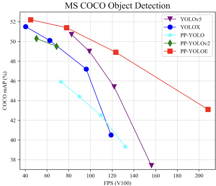
Figure 1: Comparison of the PP-YOLOE and other state-ofthe-art models. PP-YOLOE-l achieves $51.4\mathrm{mAP}$ on COCO test-dev and 78.1 FPS on Tesla V100, obtains $1.9~\mathrm{AP}$ and 9.2 FPS improvement compared with PP-YOLOv2[13].
图 1: PP-YOLOE与其他先进模型的对比。PP-YOLOE-l在COCO test-dev上达到51.4mAP,在Tesla V100上实现78.1 FPS,相比PP-YOLOv2[13]获得1.9 AP和9.2 FPS的提升。
As shown in Fig. 1, PP-YOLOE outperforms YOLOv5 and YOLOX in terms of speed and accuracy trade-off. Specifically, PP-YOLOE-l achieves $51.4\mathrm{mAP}$ on COCO with $640\times640$ resolution at the speed of 78.1 FPS, surpassing PP-YOLOv2 by $1.9%$ AP and YOLOX-l by $1.3%$ AP. Moreover, PP-YOLOE has a series of models, which can be simply configured through width multiplier and depth multiplier like YOLOv5. Our code has released on
如图 1 所示, PP-YOLOE 在速度和精度权衡方面优于 YOLOv5 和 YOLOX。具体而言, PP-YOLOE-l 在 640×640 分辨率下以 78.1 FPS 的速度在 COCO 数据集上达到 51.4mAP, 比 PP-YOLOv2 高出 1.9% AP, 比 YOLOX-l 高出 1.3% AP。此外, PP-YOLOE 拥有一系列模型, 可以像 YOLOv5 一样通过宽度乘数和深度乘数进行简单配置。我们的代码已发布在
Paddle Detection[1], with TensorRT and ONNX supported.
Paddle Detection[1], 支持 TensorRT 和 ONNX。
2. Method
2. 方法
In this section, we will first review our baseline model and then introduce the design of PP-YOLOE (Fig. 2) in detail from the aspects of network structure, label assignment strategy, head structure and loss function.
在本节中,我们将首先回顾基线模型,然后从网络结构、标签分配策略、头部结构和损失函数等方面详细介绍PP-YOLOE的设计(图2)。
2.1. A Brief Review of PP-YOLOv2
2.1. PP-YOLOv2 简述
The overall architecture of PP-YOLOv2 contains the backbone of ResNet50-vd[10] with deformable convolution[35], the neck of PAN with SPP layer and DropBlock[7] and the lightweight IoU aware head. In PPYOLOv2, ReLU activation function is used in backbone while mish activation function is used in neck. Following YOLOv3, PP-YOLOv2 only assigns one anchor box for each ground truth object. In addition to classification loss, regression loss and objectness loss, PP-YOLOv2 also uses IoU loss and IoU aware loss to boost the performance. For more details, please refer to [13].
PP-YOLOv2的整体架构包含采用可变形卷积[35]的ResNet50-vd[10]主干网络、带有SPP层和DropBlock[7]的PAN颈部结构,以及轻量化的IoU感知头部。在PP-YOLOv2中,主干网络使用ReLU激活函数,而颈部结构采用mish激活函数。遵循YOLOv3的设计,PP-YOLOv2仅为每个真实目标分配一个锚框。除分类损失、回归损失和目标存在性损失外,PP-YOLOv2还通过IoU损失和IoU感知损失来提升性能。更多细节请参阅文献[13]。
2.2. Improvement of PP-YOLOE
2.2. PP-YOLOE的改进
Anchor-free. As mentioned above, PP-YOLOv2[13] assigns ground truths in an anchor-based manner. However, anchor mechanism introduces a number of hyperparameters and depends on hand-crafted design which may not generalize well on other datasets. For the above reason, we introduce anchor-free method in PP-YOLOv2. Following FCOS[26], which tiles one anchor point on each pixel, we set upper and lower bounds for three detection heads to assign ground truths to corresponding feature map. Then, the center of bounding box is calculated to select the closest pixel as positive samples. Following YOLO series, a 4D vector (x, y, w, h) is predicted for regression. This modification makes the model a little faster with the loss of $0.3\mathrm{AP}$ as shown in Table 2. Although upper and lower bounds are carefully set according to the anchor sizes of PPYOLOv2, there are still some minor inconsistencies in the assignment results between anchor-based and anchor-free manner, which may lead to little precision drop.
无锚点机制。如前所述,PP-YOLOv2[13]采用基于锚点的方式分配真实标签。但锚点机制会引入大量超参数,且依赖人工设计,在其他数据集上可能泛化性不足。为此,我们在PP-YOLOv2中引入无锚点方法:参照FCOS[26]在每个像素点平铺单一锚点的思路,为三个检测头设置上下界来分配特征图对应的真实标签,通过计算边界框中心点选择最近像素作为正样本。延续YOLO系列传统,我们使用4D向量(x, y, w, h)进行回归预测。如表2所示,该修改使模型速度略有提升,但损失了0.3AP精度。虽然上下界是根据PP-YOLOv2锚点尺寸精心设置,但基于锚点与无锚点方式的分配结果仍存在细微差异,可能导致精度轻微下降。
Backbone and Neck. Residual connections[9, 30, 11] and dense connections[12, 15, 20] have been widely used in modern convolutional neural network. Residual connections introduce shortcut to relieve gradient vanishing prob- lem and can be also regarded as a model ensemble approach. Dense connections aggregate intermediate features with diverse receptive fields, showing good performance on the object detection task. CSPNet[28] utilizes cross stage dense connections to lower computation burden without the loss of precision, which is popular among effective object detectors such as YOLOv5[14], YOLOX[6].
骨干网络与颈部网络。残差连接 [9, 30, 11] 和密集连接 [12, 15, 20] 已被广泛应用于现代卷积神经网络中。残差连接通过引入快捷路径缓解梯度消失问题,也可视为一种模型集成方法。密集连接通过聚合具有不同感受野的中间特征,在目标检测任务中表现出优异性能。CSPNet [28] 采用跨阶段密集连接在保持精度的同时降低计算负担,该设计在YOLOv5 [14]、YOLOX [6] 等高效目标检测器中得到广泛应用。
VoVNet[15] and subsequent TreeNet[20] also show superior performance in object detection and instance segmentation. Inspired by these works, we propose a novel RepResBlock by combining the residual connections and dense connections, which is used in our backbone and neck.
VoVNet[15]及后续的TreeNet[20]在目标检测和实例分割任务中也展现出卓越性能。受这些工作启发,我们通过结合残差连接与密集连接,提出了一种新型RepResBlock结构,并将其应用于主干网络和颈部设计中。
Originating from TreeBlock[20], our Rep Res Block is shown in Fig. 3(b) during the training phase and Fig. 3(c) during the inference phase. Firstly, we simplify the original TreeBlock (Fig. 3(a)). Then, we replace the concatenation operation with element-wise add operation (Fig. 3(b)), because of the approximation of these two operations to some extent shown in RMNet [19]. Thus, during the inference phase, we can re-parameter ize s Rep Res Block to a basic residual block (Fig. 3(c)) used by ResNet-34 in a RepVGG[4] style.
源自TreeBlock[20],我们的Rep Res Block在训练阶段如图3(b)所示,在推理阶段如图3(c)所示。首先,我们简化了原始的TreeBlock (图3(a))。接着,由于RMNet[19]证明了这两种操作在某种程度上的近似性,我们将拼接操作替换为逐元素相加操作 (图3(b))。因此,在推理阶段,我们可以按照RepVGG[4]的风格将Rep Res Block重新参数化为ResNet-34使用的基础残差块 (图3(c))。
We use proposed Rep Res Block to build backbone and neck. Similar to ResNet, our backbone, named CS PRep Res Net, contains one stem composed of three convolution layer and four subsequent stages stacked by our Rep Res Block as shown in Fig. 3(d). In each stage, cross stage partial connections are used to avoid numerous parameters and computation burden brought by lots of $3~\times$ 3 convolution layers. ESE (Effective Squeeze and Extraction) layer is also used to impose channel attention in each CSP RepResS t age while building backbone. We build neck with proposed Rep Res Block and CSP RepResS t age following PP-YOLOv2[13]. Different from backbone, shortcut in Rep Res Block and ESE layer in CSP RepResS t age are removed in neck.
我们采用提出的Rep Res Block构建主干网络和颈部网络。与ResNet类似,我们的主干网络CS PRep Res Net包含一个由三个卷积层组成的stem和四个后续阶段,如图3(d)所示,这些阶段由Rep Res Block堆叠而成。在每个阶段中,采用跨阶段部分连接(cross stage partial connections)来避免大量$3~\times$3卷积层带来的参数量和计算负担。在构建主干网络时,还使用了ESE (Effective Squeeze and Extraction)层在每个CSP RepResStage中施加通道注意力。我们按照PP-YOLOv2[13]的方式,用提出的Rep Res Block和CSP RepResStage构建颈部网络。与主干网络不同,颈部网络中去除了Rep Res Block中的shortcut和CSP RepResStage中的ESE层。
We use width multiplier $\alpha$ and depth multiplier $\beta$ to scale the basic backbone and neck jointly like YOLOv5[14]. Thus, we can get a series of detection network with different parameters and computation cost. The width setting of basic backbone is [64, 128, 256, 512, 1024]. Except for the stem, the depth setting of basic backbone is [3, 6, 6, 3]. The width setting and depth setting of basic neck are [192, 384, 768] and 3 respectively. Table 1 shows the specification of width multiplier $\alpha$ and depth multiplier $\beta$ for different model. Such modifications obtains $0.7%$ AP performance improvements – $49.5%$ AP as shown in Table 2.
我们采用宽度乘数 $\alpha$ 和深度乘数 $\beta$ 联合缩放基础骨干网络和颈部结构,类似YOLOv5[14]的做法。由此可得到一系列参数量和计算成本不同的检测网络。基础骨干网络的宽度配置为[64, 128, 256, 512, 1024],除stem层外深度配置为[3, 6, 6, 3]。基础颈部结构的宽度和深度配置分别为[192, 384, 768]和3。表1展示了不同模型对应的宽度乘数 $\alpha$ 和深度乘数 $\beta$ 规格。如表2所示,这种调整带来了0.7%的AP性能提升,最终达到49.5% AP。
Table 1: Width multiplier $\alpha$ and depth multiplier $\beta$ specification for a series of networks
表 1: 一系列网络的宽度乘数 $\alpha$ 和深度乘数 $\beta$ 规格
| 宽度乘数 Q | 深度乘数 rβ | |
|---|---|---|
| S | 0.50 | 0.33 |
| m | 0.75 | 0.67 |
| 1 | 1.00 | 1.00 |
| X | 1.25 | 1.33 |
Task Alignment Learning (TAL). To further improve the accuracy, label assignment is another aspect to be considered. YOLOX uses SimOTA as the label assignment strategy to improve performance. However, to further overcome the misalignment of classification and localization, task alignment learning (TAL) is proposed in TOOD[5], which is composed of a dynamic label assignment and task aligned loss. Dynamic label assignment means prediction/loss aware. According to the prediction, it allocate dynamic number of positive anchors for each ground-truth. By explicitly aligning the two tasks, TAL can obtain the highest classification score and the most precise bounding box at the same time.
任务对齐学习 (TAL)。为进一步提升精度,标签分配是另一个需要考虑的方面。YOLOX采用SimOTA作为标签分配策略以提高性能。但为了进一步克服分类与定位的错位问题,TOOD[5]提出了任务对齐学习 (TAL),它由动态标签分配和任务对齐损失组成。动态标签分配意味着预测/损失感知,根据预测结果为每个真实标注动态分配正样本锚框。通过显式对齐这两个任务,TAL能够同时获得最高分类分数和最精确的边界框。
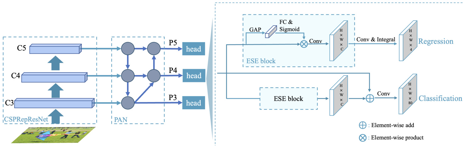
Figure 2: The model architecture of our PP-YOLOE. The backbone is CS PRep Res Net, the neck is Path Aggregation Network (PAN), and the head is Efficient Task-aligned Head (ET-head).
图 2: 我们的PP-YOLOE模型架构。主干网络是CS PRep Res Net,颈部网络是路径聚合网络 (PAN),头部网络是高效任务对齐头 (ET-head)。
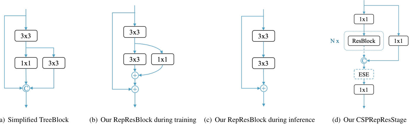
Figure 3: Structure of our Rep Res Block and CSP RepResS t age
图 3: 我们的Rep Res Block和CSP RepResStage结构
For task aligned loss, TOOD use a normalized $t$ , namely $\hat{t}$ , to replace the target in loss. It adopts the largest IoU within each instance as the normalization. The Binary Cross Entropy (BCE) for the classification can be rewritten as:
对于任务对齐损失,TOOD采用归一化的$t$(即$\hat{t}$)来替换损失中的目标值。该方法将每个实例内的最大IoU作为归一化基准。分类任务的二元交叉熵(BCE)可改写为:
$$
L_{c l s-p o s}=\sum_{i=1}^{N_{p o s}}B C E\left(p_{i},\hat{t}_{i}\right)
$$
$$
L_{c l s-p o s}=\sum_{i=1}^{N_{p o s}}B C E\left(p_{i},\hat{t}_{i}\right)
$$
We investigate the performance using different label assignment strategy. We conduct this experiment on above modified model, which use CS PRep Res Net as backbone. For get the verification results quickly, we only train 36 epochs on COCO train2017 and verify it on COCO val. As shown in Table 3, TAL achieves the best $45.2%$ AP performance. We use TAL to replace label assignment like FCOS style and achieve $0.9%$ AP improvement – $50.4%$ AP as shown in Table 2.
我们研究了使用不同标签分配策略的性能表现。实验在以上改进模型上进行,该模型采用CS PRep Res Net作为骨干网络。为快速获取验证结果,我们仅在COCO train2017上训练36个周期,并在COCO val上进行验证。如表3所示,TAL (Target-Aware Label Assignment) 取得了最佳的45.2% AP性能。我们用TAL替代FCOS风格的标签分配方式后,实现了0.9%的AP提升(如表2所示,达到50.4% AP)。
Efficient Task-aligned Head (ET-head). In object detection, the task conflict between classification and localization is a well-known problem. Corresponding solutions are proposed in many papers[5, 33, 16, 31]. YOLOX’s decoupled head draws lessons from most of the one-stage and two-stage detectors, and successfully apply to YOLO model to improve accuracy. However, the decoupled head may make the classification and localization tasks separate and independent, and lack of task specific learning. Based on
高效任务对齐头 (ET-head)。在目标检测中,分类与定位的任务冲突是一个众所周知的问题。许多论文[5, 33, 16, 31]提出了相应的解决方案。YOLOX的解耦头借鉴了多数一阶段和两阶段检测器的设计,并成功应用于YOLO模型以提高精度。然而,解耦头可能导致分类与定位任务相互分离独立,缺乏任务特异性学习。基于
Table 2: Ablation study of PP-YOLOE-l on COCO val. We use $640\times640$ resolution as input with FP32-precision, and test on Tesla V100 without post-processing.
表 2: PP-YOLOE-l 在 COCO val 上的消融实验。我们使用 $640\times640$ 分辨率作为输入,采用 FP32 精度,并在 Tesla V100 上测试(无后处理)。
| 模型 | mAP(%) | 参数量(M) | GFLOPs | 延迟(ms) | FPS |
|---|---|---|---|---|---|
| PP-YOLOv2基线模型 | 49.1 | 54.58 | 115.77 | 14.5 | 68.9 |
| +Anchor-free | 48.8 (-0.3) | 54.27 | 114.78 | 14.3 | 69.8 |
| +CSPRepResNet | 49.5(+0.7) | 47.42 | 101.87 | 11.7 | 85.5 |
| +TAL | 50.4 (+0.9) | 48.32 | 104.75 | 11.9 | 84.0 |
| +ET-head | 50.9 (+0.5) | 52.20 | 110.07 | 12.8 | 78.1 |
Table 3: Different label assignment on base model. We use CSP RepResS t age as backbone and neck, one $1\times1$ conv layer as head, and only train 36 epochs on COCO train2017.
表 3: 基础模型上的不同标签分配方法。我们使用 CSP RepResS t age 作为主干网络和颈部结构,一个 $1\times1$ 卷积层作为头部,仅在 COCO train2017 上训练 36 个周期。
| 方法 | mAP(0.5:0.95) |
|---|---|
| ATSS[34] | 43.1 |
| SimOTA[6] | 44.3 |
| TAL[5] | 45.2 |
TOOD[5], we improve the head and propose ET-head with the goal of both speed and accuracy. As shown in Fig. 2, we use ESE to replace the layer attention in TOOD, simplify the alignment of classification branches to shortcut, and replace the alignment of regression branches with distribution focal loss (DFL) layer[16]. Through the above changes, the ET-head brings an increase of $0.9\mathrm{ms}$ on V100.
TOOD[5] 中,我们对头部进行改进并提出了 ET-head,旨在兼顾速度和精度。如图 2 所示,我们使用 ESE 替代 TOOD 中的层级注意力机制,将分类分支的对齐简化为快捷连接,并将回归分支的对齐替换为分布聚焦损失 (DFL) 层[16]。通过上述改动,ET-head 在 V100 上带来了 $0.9\mathrm{ms}$ 的延迟增加。
For the learning of classification and location tasks, we choose varifocal loss (VFL) and distribution focal loss (DFL) respectively. PP-Picodet[32] successfully applys VFL and DFL in object detectors, and obtains performance improvement. For VFL in [33], different from the quality focal loss (QFL) in [16], VFL uses target score to weight the loss of positive samples. This implementation makes the contribution of positive samples with high IoU to loss relatively large. This also makes the model pay more attention to high-quality samples rather than those low-quality ones at training time. The same is that both use IoU-aware classification score (IACS) as the target to predict. This can effectively learn a joint representation of classification score and localization quality estimation, which enables high consistency between training and inference. For DFL, in order to solve the problem of inflexible representation of bounding box, [16] proposes to use general distribution to predict bounding box. Our model is supervised by the loss function:
为了分类和定位任务的学习,我们分别选择了变焦损失(VFL)和分布聚焦损失(DFL)。PP-Picodet[32]成功将VFL和DFL应用于目标检测器,并获得了性能提升。对于[33]中的VFL,与[16]中的质量聚焦损失(QFL)不同,VFL使用目标分数对正样本的损失进行加权。这种实现方式使得具有高IoU的正样本对损失的贡献相对较大。这也使得模型在训练时更关注高质量样本而非低质量样本。相同的是,两者都使用IoU感知分类分数(IACS)作为预测目标。这可以有效地学习分类分数和定位质量估计的联合表示,从而实现训练和推理之间的高度一致性。对于DFL,为了解决边界框表示不灵活的问题,[16]提出使用广义分布来预测边界框。我们的模型由以下损失函数监督:
$$
L o s s=\frac{\alpha\cdot l o s s_{V F L}+\beta\cdot l o s s_{G I o U}+\gamma\cdot l o s s_{D F L}}{\sum_{i}^{N_{p o s}}\hat{t}}
$$
$$
L o s s=\frac{\alpha\cdot l o s s_{V F L}+\beta\cdot l o s s_{G I o U}+\gamma\cdot l o s s_{D F L}}{\sum_{i}^{N_{p o s}}\hat{t}}
$$
where $\hat{t}$ denote the normalized target score, see Eq. (1). And as shown in Table 2, the ET-head obtains $0.5%$ AP improve
其中 $\hat{t}$ 表示归一化目标分数,参见公式 (1)。如表 2 所示,ET-head 实现了 $0.5%$ AP 提升
ment – 50.9% AP.
50.9% AP
3. Experiment
3. 实验
In this section, we present the experiments details and results. All experiments are trained on MS COCO-2017 training set with 80 classes and 118k images. For ablation study, we use the standard COCO AP metric with single scale on MS COCO-2017 validation set with 5000 images. And we report final results using MS COCO-2017 test-dev.
在本节中,我们将介绍实验细节与结果。所有实验均在包含80个类别、11.8万张图像的MS COCO-2017训练集上进行训练。消融研究采用标准COCO AP指标(单尺度),基于含5000张图像的MS COCO-2017验证集。最终结果通过MS COCO-2017测试开发集(test-dev)呈现。
3.1. Implementation details
3.1. 实现细节
We use stochastic gradient descent (SGD) with momen $\mathrm{tum}=0.9$ and weight decay $=5\mathrm{e}{-4}$ . We use cosine learning rate schedule, total epochs are 300, warmup epochs are 5, and base learning rate is 0.01. The total batch size is 64 on $8\times32\mathrm{GV100}$ GPU devices by default, and we follow linear scaling rule[8] to adjust learning rate. The exponential moving average (EMA) strategy with decay $=0.9998$ is also adopted during training process. We only use some basic data augmentations, including random crop, random horizontal flip, color distortion, and multi-scale. Specially, input size is evenly drawn from 320 to 768 with 32 stride.
我们使用带动量 (momentum) 为0.9的随机梯度下降 (SGD) 和权重衰减 (weight decay) 为5e-4。采用余弦学习率调度,总训练轮数为300,预热轮数为5,基础学习率为0.01。默认在8×32张GV100 GPU设备上总批次大小为64,并遵循线性缩放规则[8]调整学习率。训练过程中还采用了衰减率为0.9998的指数移动平均 (EMA) 策略。仅使用基础数据增强方法,包括随机裁剪、随机水平翻转、色彩失真和多尺度缩放。特别地,输入尺寸从320到768均匀采样,步长为32。
3.2. Comparsion with Other SOTA Detectors
3.2. 与其他SOTA检测器的对比
Table 4 and Figure 1 show comparison of the results on MS-COCO test split with other state-of-the-art object detectors. We re-evaluate YOLOv5[14] and YOLOX[6] using official codebase because they have non-scheduled updates. We compare model inference speed with batch size $=1$ (without data preprocess and non-maximum suppression). However, PP-YOLOE series using paddle inference engine. Further, for fair comparison, we also test the FP16 precision speed based on tensorRT 6.0 in the same environment. It should be emphasized that Paddle Paddle 2 officially supports tensorRT for model deployment. Therefore, PPYOLOE can use paddle inference with tensorRT directly, and other tests follow the official guidelines.
表4和图1展示了在MS-COCO测试集上与其他先进目标检测器的结果对比。我们使用官方代码库重新评估了YOLOv5[14]和YOLOX[6],因为它们存在非计划性更新。模型推理速度的比较采用批量大小$=1$(不含数据预处理和非极大值抑制)。但PP-YOLOE系列使用了Paddle推理引擎。此外,为公平起见,我们在相同环境下基于tensorRT 6.0测试了FP16精度的速度。需要强调的是,Paddle Paddle 2官方支持使用tensorRT进行模型部署,因此PPYOLOE可直接使用带tensorRT的Paddle推理,其他测试均遵循官方指南。
| 方法 | 主干网络 | 尺寸 | 无TRT FPS (v100) | 有TRT FPS (v100) | AP | AP50 | AP75 | APs | APM | APL |
|---|---|---|---|---|---|---|---|---|---|---|
| YOLOv3+ASFF*[17] | Darknet-53 | 320 | 60 | 38.1% | 57.4% | 42.1% | 16.1% | 41.6% | 53.6% | |
| YOLOv3+ASFF*[17] | Darknet-53 | 416 | 54 | 40.6% | 60.6% | 45.1% | 20.3% | 44.2% | 54.1% | |
| YOL0v4 [2] | CSPDarknet-53 | 416 | 96 | 41.2% | 62.8% | 44.3% | 20.4% | 44.4% | 56.0% | |
| YOLOv4 [2] | CSPDarknet-53 | 512 | 83 | 43.0% | 64.9% | 46.5% | 24.3% | 46.1% | 55.2% | |
| YOLOv4-CSP [27] | ModifiedCSPDarknet-53 | 512 | 97 | 46.2% | 64.8% | 50.2% | 24.6% | 50.4% | 61.9% | |
| YOLOv4-CSP [27] | Modified CSPDarknet-53 | 640 | 73 | = | 47.5% | 66.2% | 51.7% | 28.2% | 51.2% | 59.8% |
| EfficientDet-D0 [25] | Efficient-BO | 512 | 98.0 | 33.8% | 52.2% | 35.8% | 12.0% | 38.3% | 51.2% | |
| EfficientDet-D1[25] | Efficient-B1 | 640 | 74.1 | 39.6% | 58.6% | 42.3% | 17.9% | 44.3% | 56.0% | |
| EfficientDet-D2 [25] | Efficient-B2 | 768 | 56.5 | 43.0% | 62.3% | 46.2% | 22.5% | 47.0% | 58.4% | |
| EfficientDet-D2 [25] | Efficient-B3 | 896 | 34.5 | 45.8% | 65.0% | 49.3% | 26.6% | 49.4% | 59.8% | |
| PP-YOLO [18] | ResNet50-vd-dcn | 320 | 132.2+ | 242.2+ | 39.3% | 59.3% | 42.7% | 16.7% | 41.4% | 57.8% |
| PP-YOLO [18] | ResNet50-vd-dcn | 416 | 109.6+ | 215.4+ | 42.5% | 62.8% | 46.5% | 21.2% | 45.2% | 58.2% |
| PP-YOLO[18] | ResNet50-vd-dcn | 512 | 89.9+ | 188.4+ | 44.4% | 64.6% | 48.8% | 24.4% | 47.1% | 58.2% |
| PP-YOLO [18] | ResNet50-vd-dcn | 608 | 72.9+ | 155.6+ | 45.9% | 65.2% | 49.9% | 26.3% | 47.8% | 57.2% |
| PP-YOLOv2 [13] | ResNet50-vd-dcn | 320 | 123.3 | 152.9 | 43.1% | 61.7% | 46.5% | 19.7% | 46.3% | 61.8% |
| PP-YOLOv2 [13] | ResNet50-vd-dcn | 416 | 102+ | 145.1+ | 46.3% | 65.1% | 50.3% | 23.9% | 50.2% | 62.2% |
| PP-YOLOv2 [13] | ResNet50-vd-dcn | 512 | 93.4+ | 141.2+ | 48.2% | 67.1% | 52.7% | 27.7% | 52.1% | 62.1% |
| PP-YOLOv2 [13] | ResNet50-vd-dcn | 640 | 68.9+ | 106.5+ | 49.5% | 68.2% | 54.4% | 30.7% | 52.9% | 61.2% |
| PP-YOLOv2[13] | ResNet101-vd-dcn | 640 | 50.3+ | 87.0+ | 50.3% | 69.0% | 55.3% | 31.6% | 53.9% | 62.4% |
| YOLOv5-s [14] | Modified CSP v6 | 640 | 156.2+ | 454.5* | 37.4% | 56.8% | ||||
| YOL0v5-m [14] | Modified CSP v6 | 640 | 121.9+ | 263.1* | 45.4% | 64.1% | ||||
| YOL0v5-1[14] | Modified CSP v6 | 640 | 99.0+ | 172.4* | 49.0% | 67.3% | ||||
| YOLOv5-x[14] | Modified CSP v6 | 640 | 82.6+ | 117.6* | 50.7% | 68.9% | ||||
| YOLOX-s [6] | Modified CSP v5 | 640 | 119.0*|102.0+ | 246.9* | 40.5% | |||||
| YOLOX-m [6] | Modified CSP v5 | 640 | 96.1*|81.3+ | 177.3* | 47.2% | |||||
| YOL0X-1 [6] | Modified CSPv5 | 640 | 62.5*|68.9+ | 120.1* | 50.1% | |||||
| YOLOX-x [6] | Modified CSP v5 | 640 | 40.3*|57.8+ | 87.4* | 51.5% | |||||
| PP-YOLOE-S | CSPRepResNet | 640 | 208.3 | 333.3 | 43.1% | 60.5% | 46.6% | 23.2% | 46.4% | 56.9% |
| PP-YOLOE-m | CSPRepResNet | 640 | 123.4 | 208.3 | 48.9% | 66.5% | 53.0% | 28.6% | 52.9% | 63.8% |
| PP-YOLOE-1 | CSPRepResNet | 640 | 78.1 | 149.2 | 51.4% | 68.9% | 55.6% | 31.4% | 55.3% | 66.1% |
| PP-YOLOE-x | CSPRepResNet | 640 | 45.0 | 95.2 | 52.2% | 69.9% | 56.5% | 33.3% | 56.3% | 66.4% |
| PP-YOLOE+-S | CSPRepResNet | 640 | 208.3 | 333.3 | 43.7% | 60.6% | 47.9% | 26.5% | 47.5% | 59.0% |
| PP-YOLOE+-m | CSPRepResNet | 640 | 123.4 | 208.3 | 49.8% | 67.1% | 54.5% | 31.8% | 53.9% | 66.2% |
| PP-YOLOE+-1 | CSPRepResNet | 640 | 78.1 | 149.2 | 52.9% | 70.1% | 57.9% | 35.2% | 57.5% | 69.1% |
| PP-YOLOE+-x | CSPRepResNet | 640 | 45.0 | 95.2 | 54.7% | 72.0% | 59.9% | 37.9% | 59.3% | 70.4% |
Table 4: Comparison of the speed and accuracy of different object detectors on COCO 2017 test-dev. Results marked by $\because\ldots$ are updated results from the corresponding official release. Results marked by ”*” are tested in our environment using official codebase and model. The input size of YOLOv5 is not exactly square of $640\times640$ in validation and speed test, so we skip it in the table. The default precision of speed is FP32 for w/o trt and FP16 for with trt. Moreover, we provide both FP32 and FP16 for YOLOX w/o trt scene, the FP32 speed on the left side of split line and FP16 speed on the right. PP-YOLOE+ uses the model pre trained on the Objects365[24] datasets.
表 4: COCO 2017 test-dev 数据集上不同目标检测器的速度与精度对比。标记为 $\because\ldots$ 的结果来自对应官方发布的最新更新,标记为 * 的结果是在我们环境中使用官方代码库和模型测试得出。YOLOv5 在验证和速度测试时输入尺寸并非严格为 $640\times640$ 正方形,因此表中予以跳过。速度测试默认精度为:非 trt 场景使用 FP32,trt 场景使用 FP16。此外,我们为 YOLOX 非 trt 场景同时提供了 FP32 和 FP16 数据,分割线左侧为 FP32 速度,右侧为 FP16 速度。PP-YOLOE+ 使用了在 Objects365[24] 数据集上预训练的模型。