UTTERANCE WEIGHTED MULTI-DILATION TEMPORAL CONVOLUTIONALNETWORKS FOR MONAURAL SPEECH DE REVERBERATION

话语加权多膨胀时序卷积网络的单声道语音去混响

ABSTRACT

摘要

Speech de reverberation is an important stage in many speech technology applications. Recent work in this area has been dominated by deep neural network models. Temporal convolutional networks (TCNs) are deep learning models that have been proposed for sequence modelling in the task of de reverberating speech. In this work a weighted multi-dilation depthwise-separable convolution is proposed to replace standard depthwise-separable convolutions in TCN models. This proposed convolution enables the TCN to dynamically focus on more or less local information in its receptive field at each convolutional block in the network. It is shown that this weighted multi-dilation temporal convolutional network (WD-TCN) consistently outperforms the TCN across various model configurations and using the WD-TCN model is a more parameter-efficient method to improve the performance of the model than increasing the number of convolutional blocks. The best performance improvement over the baseline TCN is 0.55 dB scale-invariant signal-todistortion ratio (SISDR) and the best performing WD-TCN model attains 12.26 dB SISDR on the WHAMR dataset.

语音去混响是许多语音技术应用中的重要环节。近年来，该领域的研究主要由深度神经网络模型主导。时序卷积网络（TCN）是一种深度学习模型，被提出用于语音去混响任务中的序列建模。本研究提出了一种加权多膨胀深度可分离卷积，用于替代TCN模型中的标准深度可分离卷积。这种改进的卷积使TCN能够在网络的每个卷积块中动态调整其感受野内局部信息的关注程度。实验表明，加权多膨胀时序卷积网络（WD-TCN）在各种模型配置下均优于传统TCN，且相比增加卷积块数量，采用WD-TCN模型是更高效的参数利用方式。相较于基线TCN模型，最大性能提升达到0.55 dB尺度不变信噪比（SISDR），最优WD-TCN模型在WHAMR数据集上实现了12.26 dB的SISDR。

Index Terms— speech de reverberation, temporal convolutional network, speech enhancement, receptive field, deep neural network

索引术语 - 语音去混响 (speech dereverberation)、时序卷积网络 (temporal convolutional network)、语音增强 (speech enhancement)、感受野 (receptive field)、深度神经网络 (deep neural network)

1. INTRODUCTION

1. 引言

Speech de reverberation remains an important task for robust speech processing [1–3]. Far-field speech signals such as for automatic meeting transcription and digital assistants normally require preprocessing to remove the detrimental effects of interference in the signal [4–6]. A number of methods have been proposed for speech de reverberation for both single channel and multichannel models [7]. Recent advances in speech de reverberation performance in a number of domains have been driven by deep neural network (DNN) models [8–12].

语音去混响仍然是鲁棒语音处理的重要任务 [1-3]。远场语音信号（如自动会议转录和数字助理）通常需要预处理以消除信号中干扰的有害影响 [4-6]。针对单通道和多通道模型，已提出了多种语音去混响方法 [7]。近年来，深度神经网络 (DNN) 模型推动了多个领域语音去混响性能的进步 [8-12]。

Convolutional neural network models are commonly used for sequence modelling in speech de reverberation tasks [13–15]. One such fully convolutional model known as the TCN has been proposed for a number of speech enhancement tasks [16–18]. TCNs are capable of monaural speech de reverberation as well as more complex tasks such as joint speech de reverberation and speech separation [17]. The best performing TCN models for speech de reverberation tasks typically have a larger receptive field for data with higher reverberation times T60 and a smaller receptive field for data with small T60s [19] which forms the motivation for this paper.

卷积神经网络模型常用于语音去混响任务中的序列建模 [13-15]。其中一种全卷积模型TCN已被提出用于多项语音增强任务 [16-18]。TCN不仅能实现单通道语音去混响，还能完成更复杂的任务，如联合语音去混响与语音分离 [17]。在语音去混响任务中表现最佳的TCN模型通常对混响时间T60较长的数据采用较大感受野，而对T60较短的数据采用较小感受野 [19]，这构成了本文的研究动机。

In this work, a novel TCN architecture is proposed which is able to focus on specific temporal context within its receptive field. This is achieved by using an additional depthwise convolution kernel in the depthwise-separable convolution with a small dilation factor. Inspired by work in dynamic convolutional networks, an attention network is used to selected how to weight each of the depthwise kernels [20, 21].

本研究提出了一种新颖的TCN架构，能够在其感受野内聚焦特定时间上下文。该架构通过在深度可分离卷积中使用具有较小膨胀因子的额外深度卷积核来实现这一特性。受动态卷积网络研究的启发，我们采用注意力网络来加权每个深度卷积核 [20, 21]。

The remainder of this paper proceeds as follows. Section 2 introduces the signal model and the WD-TCN de reverberation network. Section 3 describes the experimental setup and data and results are presented in Section 4. Section 5 concludes the paper.

本文的剩余部分安排如下。第2节介绍信号模型和WD-TCN去混响网络。第3节描述实验设置，第4节展示数据和结果。第5节总结全文。

2. DE REVERBERATION NETWORK

2. 去混响网络

In this section the monaural speech de reverberation signal model is introduced and the proposed WD-TCN de reverberation model is described. The general WD-TCN model architecture is similar to the reformulation of the Conv-TasNet speech separation model [22] as a denoising auto encoder (DAE) in [19].

本节介绍了单声道语音去混响信号模型，并描述了所提出的WD-TCN去混响模型。WD-TCN的整体架构类似于将Conv-TasNet语音分离模型[22]重新表述为去噪自编码器(DAE)的方案[19]。

2.1. Signal Model

2.1. 信号模型

A reverb e rant single-channel speech signal is defined as

混响单通道语音信号定义为

$$
x[i]=h[i]\ast s[i]=s_{\mathrm{dir}}[i]+s_{\mathrm{rev}}[i]
$$

for discrete time index $i$ where $^*$ denotes the convolution operator, $h[i]$ denotes a room impulse response (RIR) and $s[i]$ denotes the clean speech signal. In this paper the target speech is $s_{\mathrm{dir}}[i]=$ $\alpha s[i-\tau]$ , i.e. the clean signal convolved with the direct path of the RIR from speaker to receiver, expressed by the delay of signal travel from speaker to receiver $\tau$ and attenuation factor $\alpha$ .

对于离散时间索引 $i$，其中 $^*$ 表示卷积运算符，$h[i]$ 表示房间脉冲响应 (RIR)，$s[i]$ 表示纯净语音信号。本文中目标语音为 $s_{\mathrm{dir}}[i]=$ $\alpha s[i-\tau]$，即纯净信号与从说话者到接收器的 RIR 直接路径卷积后的结果，由信号从说话者到接收器的传播延迟 $\tau$ 和衰减因子 $\alpha$ 表示。

The mixture signal $x[i]$ is processed in $L_{\mathbf{x}}$ blocks

混合信号 $x[i]$ 在 $L_{\mathbf{x}}$ 个块中进行处理

$$
\mathbf{x}{\ell}=[x[0.5(\ell-1)L_{\mathrm{BL}}],\ldots,x[0.5(1+\ell)L_{\mathrm{BL}}-1]]
$$

of $L_{\mathrm{BL}}$ samples with a $50%$ overlap for frame index $\ell\in{1,\ldots,L_{\mathbf{x}}}$

对于帧索引 $\ell\in{1,\ldots,L_{\mathbf{x}}}$ ，以 $50%$ 重叠率采样 $L_{\mathrm{BL}}$ 个样本

2.2. Encoder

2.2. 编码器

The encoder is a 1D convolutional layer with trainable weights $\mathbf{B}\in$ $\mathbb{R}^{L_{\mathrm{BL}}\times N}$ , where $L_{\mathrm{BL}}$ and $N$ are the kernel size and number of output channels respectively. This layer transforms $\mathbf{x}{\ell}$ into a set of filterbank features $\mathbf{w}{\ell}$ such that

编码器是一个具有可训练权重 $\mathbf{B}\in$ $\mathbb{R}^{L_{\mathrm{BL}}\times N}$ 的一维卷积层，其中 $L_{\mathrm{BL}}$ 和 $N$ 分别表示卷积核大小和输出通道数。该层将 $\mathbf{x}{\ell}$ 转换为一组滤波器组特征 $\mathbf{w}{\ell}$，使得

$$
\begin{array}{r}{\mathbf{w}{\ell}=\mathcal{H}{\mathrm{enc}}\left(\mathbf{x}_{\ell}\mathbf{B}\right),}\end{array}
$$

where $\mathcal{H}_{\mathrm{enc}}:\mathbb{R}^{1\times N}\rightarrow\mathbb{R}^{1\times N}$ is a ReLU activation function.

其中 $\mathcal{H}_{\mathrm{enc}}:\mathbb{R}^{1\times N}\rightarrow\mathbb{R}^{1\times N}$ 是一个 ReLU 激活函数。

2.3. Mask Estimation using WD-TCNs

2.3 使用 WD-TCN 进行掩码估计

A mask estimation network is trained to estimate a sequence of masks $\mathbf{m}{\ell}$ that filter the encoded features $\mathbf{w}_{\ell}$ to produce an encoded de reverberated signal defined as

训练一个掩码估计网络来估计一系列掩码 $\mathbf{m}{\ell}$，这些掩码对编码特征 $\mathbf{w}_{\ell}$ 进行滤波，从而生成定义为去混响信号的编码。

$$
\begin{array}{r}{\mathbf{v}{\ell}=\mathbf{m}{\ell}\odot\mathbf{w}_{\ell}.}\end{array}
$$

The $\odot$ operator denotes the Hadamard product. A more detailed description of the TCN used as a baseline in this paper is provided in [23]. Streaming implementations of these models are feasible but for this paper we focus on utterance-level implementations for brevity [22].

$\odot$ 运算符表示哈达玛积 (Hadamard product)。本文作为基线的 TCN 更详细描述见 [23]。这些模型的流式实现是可行的，但为了简洁起见，本文主要关注话语级实现 [22]。

The conventional TCN consists of an initial stage which normalizes the encoded features $\mathbf{w}_{\ell}$ and reduces the number of features from $N$ to $B$ for each block using a pointwise convolution (P-Conv) bottleneck layer [22]. The TCN is composed of a stack of $X$ dilated convolutional blocks that is repeated $R$ times. This structure allows for increasingly larger models with increasingly larger receptive fields [19]. The depthwise convolution (D-Conv) layer in the blocks has an increasing dilation factor to the power of two for the $X$ blocks in a stack, i.e. the dilation factors $f$ for each block are taken from the set ${2^{0},2^{1},\dots,2^{X-1}}$ in increasing order. Fig. 1 (a) depicts the convolutional block as implemented in [23,24]. The convolutional block consist primarily of P-Conv and D-Conv layers with parametric rectified linear unit (PReLU) activation functions [25] and global layer normalization (gLN) layers [22]. The P-Conv and D-Conv layers are structured to allow increasingly larger models to have larger receptive fields. Combining these two operations is an operation known as depthwise-separable convolution (DS-Conv) [22]. More detailed definitions of P-Conv, D-Conv and DS-Conv layers are given in Section 2.3.1 before the proposed WD-TCN to replace the DS-Conv operations in TCNs is introduced in Section 2.3.2, denoted in this paper as weighted multi-dilation depthwise-separable convolution (WD-Conv).

传统的TCN由一个初始阶段组成，该阶段通过逐点卷积 (P-Conv) 瓶颈层 [22] 对编码特征 $\mathbf{w}_{\ell}$ 进行归一化，并将每个块的特征数量从 $N$ 减少到 $B$。TCN由 $X$ 个扩张卷积块堆叠而成，并重复 $R$ 次。这种结构使得模型可以随着感受野的增大而扩展 [19]。块中的深度卷积 (D-Conv) 层对堆叠中的 $X$ 个块采用以2为底的指数递增扩张因子，即每个块的扩张因子 $f$ 取自集合 ${2^{0},2^{1},\dots,2^{X-1}}$ 并按递增顺序排列。图1(a)展示了文献 [23,24] 中实现的卷积块结构。该卷积块主要由P-Conv和D-Conv层构成，并采用参数化修正线性单元 (PReLU) 激活函数 [25] 和全局层归一化 (gLN) 层 [22]。P-Conv和D-Conv层的结构设计使得更大的模型能够拥有更大的感受野。这两种操作的组合被称为深度可分离卷积 (DS-Conv) [22]。第2.3.1节将详细定义P-Conv、D-Conv和DS-Conv层，随后在第2.3.2节提出用加权多扩张深度可分离卷积 (WD-Conv) 替代TCN中的DS-Conv操作。

2.3.1. Depthwise-Separable Convolution (DS-Conv)

2.3.1. 深度可分离卷积 (DS-Conv)

The DS-Conv operation is a factorised version of standard convolutional kernel using a D-Conv layer and a P-Conv layer. The main motivation for using DS-Conv is primarily parameter efficiency where the number of channels is sufficiently larger than the kernel size [22]. Note that in this section the focus is entirely on 1D convolutional kernels but the same principle can be extended to higher dimensional kernels.

DS-Conv操作是标准卷积核的分解版本，使用D-Conv层和P-Conv层。采用DS-Conv的主要动机是参数效率，即当通道数远大于卷积核尺寸时的优化方案 [22]。需要注意的是，本节完全聚焦于一维卷积核，但相同原理可推广到更高维度的卷积核。

The D-Conv layer is an entirely sequential convolution with dilation factor $f$ , i.e. each operation operates on each input channel individually. For the matrix of input features $\mathbf{Y}\in\mathbb{R}^{G\times\hat{L}_{\mathbf{x}}}$ where $G$ is the number of input channels (and consequently also the number of output channels) the D-Conv operation can be defined as

D-Conv层是一种完全序列化的卷积操作，其膨胀因子为$f$，即每个操作独立作用于每个输入通道。对于输入特征矩阵$\mathbf{Y}\in\mathbb{R}^{G\times\hat{L}_{\mathbf{x}}}$（其中$G$表示输入通道数，同时也是输出通道数），D-Conv运算可定义为

$$
\mathcal{D}(\mathbf{Y},\mathbf{K}{\mathcal{D}})=\left[\left(\mathbf{y}{0}\mathbf{k}{0}\right)^{\top},\ldots,\left(\mathbf{y}{G-1}*\mathbf{k}_{G-1}\right)^{\top}\right]^{\top}
$$

where ${\bf K}{\mathcal{D}}\in\mathbb{R}^{G\times P}$ is the the D-Conv kernel matrix of trainable weights and $P$ is the kernel size. The $g$ th row of $\mathbf{Y}$ and ${\bf K}{\mathcal{D}}$ are denoted by ${\mathbf y}{g}$ and ${\bf k}{g}$ respectively.

其中 ${\bf K}{\mathcal{D}}\in\mathbb{R}^{G\times P}$ 是可训练权重的 D-Conv 核矩阵，$P$ 是核大小。$\mathbf{Y}$ 和 ${\bf K}{\mathcal{D}}$ 的第 $g$ 行分别表示为 ${\mathbf y}{g}$ 和 ${\bf k}_{g}$。

The P-Conv layer is an entirely channel-wise convolution. This operation in practice is a standard 1D convolutional kernel but with only a kernel size of 1. The P-Conv operation can be defined as

P-Conv层是一种完全通道维度的卷积操作。该操作在实践中是一个标准的一维卷积核，但仅具有1的核大小。P-Conv操作可以定义为

$$
\mathcal{P}(\mathbf{Y},\mathbf{K}{\mathcal{P}})=\mathbf{Y}^{\top}\mathbf{K}_{\mathcal{P}}
$$

where ${\bf K}_{\mathcal{P}}\in\mathbb{R}^{G\times H}$ is the P-Conv kernel of trainable weights.

其中 ${\bf K}_{\mathcal{P}}\in\mathbb{R}^{G\times H}$ 是可训练权重的 P-Conv 核。

Combining the definitions for the D-Conv and P-Conv operations, the DS-Conv operation is defined as

结合 D-Conv 和 P-Conv 操作的定义，DS-Conv 操作定义为

$$
\begin{array}{r}{S\left(\mathbf{Y},\mathbf{K}{\mathcal{D}},\mathbf{K}{\mathcal{P}}\right)=\mathcal{P}\left(\mathcal{D}\left(\mathbf{Y},\mathbf{K}{\mathcal{D}}\right),\mathbf{K}_{\mathcal{P}}\right).}\end{array}
$$

The DS-Conv operation as implemented in the baseline system used in [19] and in this paper can be seen in Fig. 1 (a) highlighted by the dashed orange box.

图 1 (a) 中用橙色虚线框标出的部分展示了[19]及本文采用的基线系统中实现的DS-Conv操作。

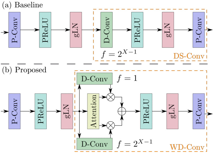
Fig. 1: (a) Convolutional block in baseline TCN; (b) Proposed convolutional block. Example for final block in a stack of conv. blocks for $Q:=:2$ with dilation factor $f=2^{X-1}$ . Note that a residual connection around the entire block is omitted for brevity.

图 1: (a) 基准 TCN 中的卷积块; (b) 提出的卷积块。示例展示了 $Q:=:2$ 且扩张因子 $f=2^{X-1}$ 时, 卷积块堆栈中最终块的结构。为简洁起见, 图中省略了环绕整个块的残差连接。

2.3.2. Weighted Multi-Dilation Depthwise-Separable Convolution (WD-Conv)

2.3.2. 加权多膨胀深度可分离卷积 (WD-Conv)

The WD-Conv network structure depicted in Fig. 1 (b) is proposed here as an extension to the DS-Conv operation where it is preferable to allow the network to be more selective about the temporal context to focus on without drastically increasing the number of parameters in the model. The proposed WD-Conv layer incorporates additional parallel D-Conv layers that can have a different dilation factor, hence it is referred to as dilation-augmented. The output of the D-Conv layers are weighted in a sum-to-one fashion and summed together. This summed output is then passed as the input to a P-Conv. In its simplest form the WD-Conv operation can be formulated as

图 1 (b) 所示的 WD-Conv 网络结构是对 DS-Conv 操作的扩展，其优势在于允许网络更灵活地选择需要关注的时间上下文，而不会显著增加模型参数量。该 WD-Conv 层通过引入具有不同膨胀系数的并行 D-Conv 层实现功能增强（称为膨胀增强机制），各 D-Conv 层输出按总和为一的权重进行加权求和，最终将加权结果输入 P-Conv。其基础运算公式可表示为

$$
\begin{array}{l}{{\displaystyle\mathcal{W}\left({\bf Y},\left({\bf K}{\mathcal{D}{1},\mathcal{I}},\ldots,{\bf K}{\mathcal{D}{Q}}\right),{\bf K}{\mathcal{P}}\right)=}}\ {{\displaystyle\mathcal{P}\left(\sum_{q=1}^{Q}a_{q}\mathcal{D}{q}\left({\bf Y},{\bf K}{\mathcal{D}{q}}\right),{\bf K}_{\mathcal{P}}\right)}}\end{array}
$$

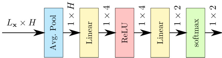
Fig. 2: Squeeze and excite attention weighting network. Output dimens ional it y of each layer is indicated above arrows.

图 2: 压缩激励注意力加权网络。各层输出维度标注于箭头上方。

Inspired by the dynamic convolution kernel proposed in [21], the implementation proposed in this paper computes the weights for each D-Conv layer using an squeeze-and-excite (SE) attention network [26]. The SE attention network is shown in Fig. 2 and is composed of a global average pooling layer that reduces the sequence dimension from $L_{\mathbf{x}}$ to 1 producing a vector of dimension $H$ , the same as the feature dimension of the input. This feature vector is then compressed using a linear layer, with a rectified linear unit (ReLU) activation, to a dimension of 4 as in [21]. The final stage is a linear layer that computes a weight for each of the D-Conv kernels in the WD-Conv structure. In the proposed model there are two D-Conv kernels and so the linear layer has an input dimension of 4 and an output dimension of 2. A softmax activation is used to ensure the sum-to-one constraint on the weights of the D-Conv layers.

受[21]中提出的动态卷积核启发，本文提出的实现方案采用压缩激励(SE)注意力网络[26]计算每个D-Conv层的权重。如图2所示，SE注意力网络由全局平均池化层构成，该层将序列维度从$L_{\mathbf{x}}$降至1，生成维度为$H$的向量（与输入特征维度相同）。随后通过带ReLU激活函数的线性层将该特征向量压缩至4维（如[21]所述）。最终阶段通过线性层为WD-Conv结构中的每个D-Conv核计算权重。该模型包含两个D-Conv核，因此线性层输入维度为4，输出维度为2。采用softmax激活函数确保D-Conv层权重满足总和为一的约束条件。

2.4. Decoder

2.4. 解码器

The decoder tansforms the encoded de reverberated signal $\mathbf{v}{\ell}$ back into a time domain signal using a transposed 1D convolutional layer with $N$ input channels, 1 output channel and a kernel size of $L_{\mathrm{BL}}$ such that

解码器通过一个转置的1D卷积层将编码的去混响信号 $\mathbf{v}{\ell}$ 转换回时域信号，该卷积层具有 $N$ 个输入通道、1个输出通道和 $L_{\mathrm{BL}}$ 的核大小，使得

$$
\hat{\mathbf{s}}{\ell}=\mathbf{v}_{\ell}\mathbf{U}
$$

where $\mathbf{U}\in\mathbb{R}^{N\times L_{\mathrm{BL}}}$ is a matrix of trainable convolutional weights and $\hat{\mathbf{s}}_{\ell}$ is an estimated de reverberated signal block in the time domain. The overlap-add method is used for re-synthesis of the signal from the overlapping blocks.

其中 $\mathbf{U}\in\mathbb{R}^{N\times L_{\mathrm{BL}}}$ 是可训练卷积权重矩阵，$\hat{\mathbf{s}}_{\ell}$ 是时域中估计的去混响信号块。采用重叠相加法从重叠块中重新合成信号。

2.5. Objective Function

2.5. 目标函数

The objective function used here is the SISDR function [27] which is the same as that used to train the baseline TCN [19]. It is reformulated as a loss function by taking the negative SISDR value between the estimated speech segment S and the reference direct path of the signal $\mathbf{s}_{\mathrm{dir}}$ defined as

此处使用的目标函数是SISDR函数[27]，与用于训练基准TCN[19]的函数相同。通过计算估计语音段S与信号参考直达路径$\mathbf{s}_{\mathrm{dir}}$之间的负SISDR值，将其重新表述为损失函数。

$$
\mathcal{L}{\mathrm{SISDR}}(\hat{\mathbf{s}},\mathbf{s}{\mathrm{dir}}):=-10\log_{10}\frac{\left|\left|\frac{\langle\hat{\mathbf{s}},\mathbf{s}{\mathrm{dir}}\rangle\mathbf{s}{\mathrm{dir}}}{|\mathbf{s}{\mathrm{dir}}|^{2}}\right|\right|^{2}}{\left|\hat{\mathbf{s}}-\frac{\langle\hat{\mathbf{s}},\mathbf{s}{\mathrm{dir}}\rangle\mathbf{s}{\mathrm{dir}}}{|\mathbf{s}_{\mathrm{dir}}|^{2}}\right|^{2}}.
$$

3. EXPERIMENTAL SETUP

3. 实验设置

3.1. Model and Training Configuration

3.1. 模型与训练配置

Different model configurations are compared in the following to demonstrate the improvement gained by the proposed WD-TCN model across a range of model sizes. This is done by varying the number of convolutional blocks in a dilated stack $X$ as well as the number of times the dilated stack is repeated $R$ . Based on previous work [19], the ranges of $X\in{4,5,6,7,8}$ and $R\in{4,5,6,7,8}$ were selected, resulting in 25 different configurations. All other parameters are fixed, i.e. kernel size $L_{\mathrm{BL}}=16$ , number of encoder output channels $N=512$ , number of bottleneck output channels $B=128$ , number of channels inside the convolutional blocks $H=512$ and the kernel size inside each D-Conv $P=3$ . For more details on these parameters see [19, 22, 23].

以下比较不同模型配置，以展示所提出的WD-TCN模型在一系列模型规模上的改进效果。通过调整扩张堆栈中的卷积块数量$X$以及扩张堆栈的重复次数$R$来实现。基于先前工作[19]，选定$X\in{4,5,6,7,8}$和$R\in{4,5,6,7,8}$的范围，共产生25种不同配置。其余参数固定：卷积核大小$L_{\mathrm{BL}}=16$、编码器输出通道数$N=512$、瓶颈层输出通道数$B=128$、卷积块内部通道数$H=512$以及每个D-Conv内部卷积核大小$P=3$。更多参数细节详见[19, 22, 23]。

The same training approach as in [19] is used for both the baseline TCN and WD-TCN. Each model is trained for 100 epochs. An initial learning rate of 0.001 is used and is halved if there is no improvement for 3 epochs. A batch size of 4 is used. The training was performed using the Speech Brain speech processing toolkit [24]. The implementation of the proposed WD-TCN is available on GitHub1.

基线TCN和WD-TCN均采用与[19]相同的训练方法。每个模型训练100个周期，初始学习率为0.001，若连续3个周期无改进则学习率减半，批处理大小为4。训练使用Speech Brain语音处理工具包[24]完成。WD-TCN的实现代码已发布于GitHub1。

3.2. Data

3.2. 数据

The simulated WHAMR noisy reverb e rant two speaker speech separation corpus [16] is used for the following experiments in this section. Only the reverb e rant and clean first speaker data is used for the input data $x[i]$ and target data $s_{\mathrm{dir}}[i]$ . RIRs are simulated using the py room acoustics software toolkit [28] and then convolved with the speech clips to produce the reverb e rant signal $x[i]$ . The training set contains 20,000 samples for training which are truncated or padded to $4\mathrm{s~}$ in length, to address sample length mismatches in batches and to also speed up training. There are 5000 samples $(14.65~\mathrm{hrs})$ and 3000 samples (9 hrs) in the validation and test sets respectively.

本节后续实验采用模拟的WHAMR含噪混响双说话人语音分离语料库[16]。仅使用混响语音和干净的第一说话人数据分别作为输入数据$x[i]$和目标数据$s_{\mathrm{dir}}[i]$。通过pyroomacoustics软件工具包[28]模拟房间脉冲响应(RIR)，再与语音片段卷积生成混响信号$x[i]$。训练集包含20,000个样本，所有样本被截断或填充至$4\mathrm{s}$统一长度，以解决批次样本长度不匹配问题并加速训练。验证集和测试集分别包含5000个样本$(14.65~\mathrm{小时})$和3000个样本(9小时)。

3.3. Metrics

3.3. 指标

A number of metrics are used to assess a variety of properties in the de reverberated speech. The objective function SISDR is also used to measure distortions in signals. Speech-to-reverberation modulation energy ratio (SRMR) [29] is a measure used to directly measure reverb e rant effects in the signal. Perceptual evaluation of speech quality (PESQ) [30] and extended short-time objective in tell i gibi lity (ESTOI) [31] are objective measures used to assess the quality and intelligibility of signals.

多种指标用于评估去混响语音的各种特性。目标函数SISDR也被用来测量信号失真。语音-混响调制能量比(SRMR) [29]是一种直接测量信号中混响效应的指标。语音质量感知评估(PESQ) [30]和扩展短时客观可懂度(ESTOI) [31]是用于评估信号质量和可懂度的客观测量方法。

4. RESULTS

4. 结果

4.1. Performance Metrics and Model Size

4.1. 性能指标与模型规模

The average SISDR results on the WHAMR evaluation set for the 25 chosen model configurations of the proposed WD-TCN model are given in Table 1 with SISDR improvements over the TCN model in the parenthesis. The bold font indicates best performance and highest improvement, respectively. These results show that the WD-TCN outperforms the TCN model across all 25 model configurations. The biggest performance gains are seen around ${X,R}=$ ${5,7}$ and the WD-TCN model with most parameters and largest receptive field, ${X,R}={8,8}$ , shows best overall performance, contrary to the TCN model which gave the best SISDR results with ${X,R}={6,8}$ . Fig. 3 (top) shows SISDR performance for all models over the model sizes in number of parameters. It can be seen that using the WD-TCN is a more parameter efficient approach to improving model performance than increasing the number of convolutional blocks (larger $X$ or $R$ values) in a conventional TCN. The SRMR performance against model size (Fig. 3, lower panel) shows the same findings, i.e. that the WD-TCN is a more parameter efficient approach to improving performance. For some larger models $(>6\mathrm{M}$ parameters) performance differs less. However the best performing model in terms of SRMR is still the WD-TCN.

所提出的WD-TCN模型在WHAMR评估集上25种选定配置的平均SISDR结果如表1所示，括号内为相较TCN模型的SISDR提升量。加粗字体分别表示最佳性能和最高改进幅度。结果表明，WD-TCN在所有25种模型配置中均优于TCN模型。最大性能增益出现在${X,R}=$${5,7}$附近，而参数量最多、感受野最大的WD-TCN配置${X,R}={8,8}$展现出最佳整体性能——这与TCN模型的最佳SISDR结果出现在${X,R}={6,8}$的情况相反。图3（上）展示了所有模型SISDR性能随参数量变化的趋势，可见相较于传统TCN通过增加卷积块数量（更大的$X$或$R$值），采用WD-TCN是更高效的参数利用方案。SRMR性能与模型规模的关系（图3下）呈现相同结论，即WD-TCN能以更少参数实现性能提升。部分较大模型$(>6\mathrm{M}$参数)的性能差异较小，但SRMR指标下的最佳表现仍由WD-TCN保持。

1Link to WD-TCN model on GitHub: https://github.com/ jwr1995/WD-TCN Table 1: SISDR performance of WD-TCN with SE attention in dB. Numbers in (·) report performance improvement over baseline TCN.

WD-TCN模型GitHub链接：https://github.com/jwr1995/WD-TCN
表1: 采用SE注意力机制的WD-TCN在SISDR指标上的性能表现(dB)。括号内数值表示相比基准TCN的性能提升。

		X
		5	6	7	8
	4	11.21 (.28)	11.66 (.29)	11.81 (.40)	11.94 (.38)
R	5 6 7	11.51 (.41) 11.64 (.38) 11.65 (.20) 11.79 (.27) 12.03 (.19)	11.86 (.41) 11.95 (.30) 12.17 (.44)	11.94 (.23) 12.08 (.31) 12.22 (.30)	12.11 (.42) 12.09 (.23) 12.16 (.13)

Fig. 3: Comparison of baseline TCN and WD-TCN over model size (no. of parameters) in terms of SISDR (top) and SRMR (bottom).

图 3: 基线 TCN 与 WD-TCN 在模型参数量上的 SISDR (上) 和 SRMR (下) 对比。

Table 2 shows the results of the best performing TCN and WD-TCN models for each of the chosen performance metrics, highlighted in yellow, compared with the respective other model for the same $X$ and $R$ hyper-parameters. The performance in PESQ is inconclusive as many TCN models outperform their corresponding WD-TCN configurations but the best PESQ score of 3.5 is achieved with the WD-TCN model. The WD-TCN models show slightly better performance in ESTOI in line with the trend already observed in SRMR and SISDR. Note that SRMR is considered the most significant metric as it is designed to assess reverberation only.

表 2 展示了在选定性能指标下表现最佳的 TCN 和 WD-TCN 模型结果 (黄色高亮) ，并与相同 $X$ 和 $R$ 超参数下的另一种模型进行对比。PESQ 指标结果尚无定论，因为许多 TCN 模型优于对应的 WD-TCN 配置，但 WD-TCN 模型取得了 3.5 的最高 PESQ 分数。WD-TCN 模型在 ESTOI 上表现略优，这与 SRMR 和 SISDR 指标中已观察到的趋势一致。需注意 SRMR 被视为最重要的指标，因为其设计初衷是仅评估混响效果。

4.2. Squeeze-and-Excite Attention Analysis and T60 Variation

4.2. 压缩激励注意力分析与T60变化

In the following, the attentive weights $a_{q}$ in (8) in the convolutional blocks are analysed. Note that $a_{1}$ corresponds to the attention weight applied to the D-Conv layers with the increasing dilation of $f\in{1,\hat{2},\dots,2^{X-1}}$ for all convolutional blocks (cf. Fig. 1 (b)) and $a_{2}=$ is the weight corresponding to the D-Conv layers with the more local fixed dilation $f=1$ . To analyse whether the SE attention approach was working as intended the attention weights were firstly computed across the entire evaluation set for every WD-TCN model trained in Table 1. Mean values of the weights for each model and each sample in the evaluation set were then computed and the evaluation set was in divided into increasing T60 ranges from 0.1s up to 1s. The mean for each weight $a_{q}$ over all models and samples, denoted as $\bar{a}{q},q\in{1,2}$ , was then computed for each T60 range. Figure 4 shows how the mean weight values vary across increasing T60 ranges. As the T60 range increases $\bar{a}{1}$ increases. This demonstrates the SE attention approach is working as intended because the network has a less local focus within its receptive field for speech signals with larger reverberation times. Similarly the mean of the local attention weight $\bar{a}_{2}$ decreases as the T60 range increases demonstrating that the network is more focused on local information in its receptive field when the speech has a smaller reverberation time.

以下分析卷积块中(8)式的注意力权重$a_{q}$。需注意，$a_{1}$对应所有卷积块中采用递增扩张率$f\in{1,\hat{2},\dots,2^{X-1}}$的D-Conv层注意力权重（参见图1(b)），而$a_{2}$对应采用固定局部扩张率$f=1$的D-Conv层权重。为验证SE注意力机制是否按预期工作，首先计算了表1中所有训练完成的WD-TCN模型在整个评估集上的注意力权重，随后计算每个模型在评估集中各样本的权重均值，并将评估集按T60值从0.1秒至1秒划分为递增区间。对每个T60区间，计算所有模型和样本的权重均值$\bar{a}{q},q\in{1,2}$。图4展示了不同T60区间内均值权重的变化趋势：随着T60区间增大，$\bar{a}{1}$持续上升，这表明SE注意力机制运作符合预期——当语音信号混响时间较长时，网络会减少对其感受野内局部信息的关注；相应地，局部注意力权重均值$\bar{a}_{2}$随T60区间增大而下降，说明当语音混响时间较短时，网络会更聚焦于感受野中的局部信息。

Table 2: Best performing TCN and WD-TCN models compared corresponding models in SISDR, PESQ, ESTOI and SRMR. Bold indicates best performance per configuration, in terms of the $X$ and $R$ hyper-parameters. Results highlighted in yellow indicate best overall results for each model in each metric.

表 2: 性能最佳的 TCN 和 WD-TCN 模型在 SISDR、PESQ、ESTOI 和 SRMR 指标上与对应模型的比较。加粗表示在 $X$ 和 $R$ 超参数配置下的最佳性能，黄色高亮表示每个模型在各指标中的整体最佳结果。

模型	X	R	#params	SISDR	PESQ	ESTOI	SRMR
TCN WD-TCN	6 6	7 7	5.8M 6.0M	11.92 12.22	3.46 3.5	0.930 0.933	8.65
TCN	6	8	6.6M	12.03	3.46	0.932	8.69 8.70
WD-TCN TCN	6 8	8 4	6.8M 4.5M	12.20 11.63	3.43 3.48	0.934 0.927	8.72 8.60
WD-TCN	8	4	4.6M	12.04	3.45	0.931	8.67
TCN WD-TCN	8 8	7 7	7.7M 7.9M	11.98 12.14	3.46 3.45	0.933 0.935	8.79 8.72

Fig. 4: Mean values of attention weights $\overline{{{a}}}_{q}$ across six different T60 ranges in the WHAMR evaluation set over all models with $X\in$ ${4,\ldots,8}$ and $R\in{4,\ldots,8}$ .

图 4: WHAMR评估集中所有模型在六个不同T60范围内的注意力权重均值$\overline{{{a}}}_{q}$，其中$X\in{4,\ldots,8}$且$R\in{4,\ldots,8}$。

5. CONCLUSIONS

5. 结论

In this work, the WD-TCN model was proposed for TCN-based speech de reverberation by replacing depthwise-separable convolutions with weight multi-dilation depthwise-separable convolutions. It was shown that the WD-TCN consistently outperformed a conventional TCN across 25 different model configurations and that using the WD-TCN was a more parameter efficient approach to improving model performance than increasing the number of convolutional blocks in the TCN.

本研究提出WD-TCN模型用于基于TCN的语音去混响任务，通过将深度可分离卷积替换为权重多膨胀深度可分离卷积。实验表明，在25种不同模型配置下，WD-TCN始终优于传统TCN，且相比增加TCN中卷积块数量，采用WD-TCN是更高效的参数利用方式。

[论文翻译]话语加权多膨胀时序卷积网络的单声道语音去混响

原文地址：https://arxiv.org/pdf/2205.08455v3