TF-LOCOFORMER: TRANSFORMER WITH LOCAL MODELING BY CONVOLUTIONFOR SPEECH SEPARATION AND ENHANCEMENT
TF-LOCOFORMER: 基于卷积局部建模的Transformer语音分离与增强模型
ABSTRACT
摘要
Time-frequency (TF) domain dual-path models achieve high-fidelity speech separation. While some previous state-of-the-art (SoTA) models rely on RNNs, this reliance means they lack the parallelizability, s cal ability, and versatility of Transformer blocks. Given the wide-ranging success of pure Transformer-based architectures in other fields, in this work we focus on removing the RNN from TF-domain dual-path models, while maintaining SoTA performance. This work presents TF-Locoformer, a Transformer-based model with LOcal-modeling by COnvolution. The model uses feedforward networks (FFNs) with convolution layers, instead of linear layers, to capture local information, letting the self-attention focus on capturing global patterns. We place two such FFNs before and after self-attention to enhance the local-modeling capability. We also introduce a novel normalization for TF-domain dual-path models. Experiments on separation and enhancement datasets show that the proposed model meets or exceeds SoTA in multiple benchmarks with an RNN-free architecture.
时频 (TF) 域双路径模型实现了高保真语音分离。虽然之前的一些最先进 (SoTA) 模型依赖于 RNN,但这种依赖意味着它们缺乏 Transformer 模块的可并行性、可扩展性和通用性。鉴于纯 Transformer 架构在其他领域的广泛成功,本工作的重点是在保持 SoTA 性能的同时,从 TF 域双路径模型中移除 RNN。本文提出了 TF-Locoformer,这是一种基于 Transformer 的模型,通过卷积实现局部建模 (LOcal-modeling by COnvolution)。该模型使用带有卷积层的前馈网络 (FFN) 代替线性层来捕获局部信息,使自注意力专注于捕获全局模式。我们在自注意力前后放置了两个这样的 FFN 以增强局部建模能力。我们还为 TF 域双路径模型引入了一种新颖的归一化方法。在分离和增强数据集上的实验表明,所提出的模型在多个基准测试中达到或超过了 SoTA,且无需 RNN 架构。
Index Terms— speech separation, self-attention, convolution
索引术语— 语音分离 (speech separation), 自注意力 (self-attention), 卷积 (convolution)
1. INTRODUCTION
1. 引言
The past decade has witnessed dramatic progress in speech separation thanks to advancements in neural networks (NNs). Early work such as deep clustering [1] trains NNs to estimate time-frequency (TF) masks in the TF-magnitude domain. In contrast, time-domain audio separation network (TasNet)-style NNs have improved separation performance drastically by introducing learnable encoders and decoders [2]. Dual-path modeling, which chunks the features and conducts local and global modeling alternately for efficient sequence modeling, is now one of the mainstream approaches in time-domain end-to-end (E2E) networks [3–5]. More recently, dual-path modeling in the TF domain, where temporal and frequency modeling are done alternately, has shown impressive performance improvements [6, 7]. TF-domain models have the potential to perform better in realistic reverb e rant conditions, as the FFT window size is usually much longer than the kernel size of a typical learnable encoder [8].
过去十年,神经网络(NN)的进步推动了语音分离领域的显著发展。早期工作如深度聚类(deep clustering) [1] 训练神经网络在时频(TF)幅度域估计时频掩码。相比之下,时域音频分离网络(TasNet)类模型通过引入可学习编码器/解码器 [2] 大幅提升了分离性能。双路径建模(dual-path modeling)通过分块特征并交替进行局部和全局建模来实现高效序列建模,现已成为时域端到端(E2E)网络的主流方法之一 [3–5]。最近,在时频域交替进行时间和频率建模的双路径方法 [6,7] 展现出卓越的性能提升。时频域模型在实际混响环境中可能表现更优,因为FFT窗口尺寸通常远大于典型可学习编码器的核尺寸 [8]。
While Transformer-based architectures [9] have shown great success in time-domain E2E separation [5, 10, 11], the current state-of-the-art (SoTA) TF-domain dual-path separation model relies on RNNs [7]. Although RNNs have some advantages such as smaller memory cost in inference, the training is typically very time-consuming since it cannot be parallel i zed. In contrast, Transformer-based models have been eagerly investigated in other fields [9, 12, 13] because of their multiple advantages: the training process can be parallel i zed, models can accept prompts (e.g., to specify the task [14,15]), and they may scale well [16–18]; these features are either unattainable or at least unconfirmed in RNNs. Before realizing these potential benefits of Transformer-based models, the first step, which is the goal of this paper, is to investigate whether we can obtain comparable or better performance as RNN-based SoTA models with an RNN-free model of similar complexity.
基于Transformer的架构[9]在时域端到端(E2E)分离任务中已展现出卓越性能[5,10,11],但当前最先进的时频域(TF-domain)双路径分离模型仍依赖循环神经网络(RNN)[7]。虽然RNN具有推理内存占用较小等优势,但由于无法并行化,其训练过程通常非常耗时。相比之下,基于Transformer的模型因其多重优势在其他领域被广泛研究[9,12,13]:训练过程可并行化、模型能接收提示(例如指定任务[14,15])、以及良好的扩展性[16-18];这些特性在RNN中要么无法实现,至少尚未得到证实。在实现Transformer模型这些潜在优势之前,本文的首要目标是探究:在模型复杂度相近且不含RNN的情况下,能否取得与基于RNN的最先进模型相当或更优的性能。
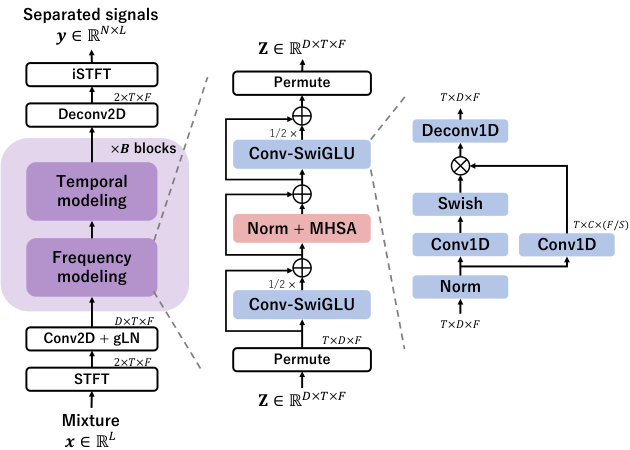
Fig. 1. Overview of the proposed TF-Locoformer. The temporal modeling block is the same as the frequency modeling block with a permutation of the time and frequency dimensions.
图 1: 提出的 TF-Locoformer 概览。时序建模模块与频域建模模块结构相同,仅对时间和频率维度进行置换。
Global and local modeling often both play an important role in speech processing [19]. There are strong hints in the literature that this is also true for speech separation, and that Transformer blocks lack an intrinsic local modeling ability. Indeed, Transformer blocks, which excel at global modeling thanks to self-attention, have worked well in the context of time-domain dual-path models [5], where selfattention in the intra-chunk path is limited to local modeling by construction, while failing to compete in TF-domain dual-path architectures, where local modeling is not explicitly enforced. On the other hand, RNNs, which can capture local information, do attain strong performance in TF-domain dual-path models. Notably, the current SoTA model in TF-domain separation, TF-GridNet [7], exploits both RNNs and self-attention. As an alternative to RNNs for capturing local information, we consider inserting convolution layers within a Transformer-based dual-path architecture.
全局和局部建模在语音处理中通常都扮演着重要角色 [19]。文献中有强烈暗示表明,这一规律同样适用于语音分离任务,且Transformer模块本身缺乏固有的局部建模能力。事实上,凭借自注意力机制擅长全局建模的Transformer模块,在时域双路径模型 [5] 中表现优异(其段内路径的自注意力通过结构设计被限制为局部建模),却在时频域双路径架构中未能取得竞争力(该架构未显式强制局部建模)。另一方面,能够捕捉局部信息的循环神经网络 (RNN) 确实在时频域双路径模型中实现了强劲性能。值得注意的是,当前时频域分离的最先进模型TF-GridNet [7] 就同时采用了RNN和自注意力机制。作为捕捉局部信息的RNN替代方案,我们考虑在基于Transformer的双路径架构中插入卷积层。
We propose TF-Locoformer (TF-domain Transformer with LOcal modeling by COnvolution), a simple extension of the Transformerbased model that alternates global and local modeling. Starting from the normal Transformer block, we first replace the two linear layers in the feed-forward network (FFN) with 1d-convolution and 1dde convolution layers, respectively. In addition, we leverage swish gated linear unit (SwiGLU) activation s in the FFNs and place such FFNs both before and after self-attention, inspired by the success of the macaron-style architecture [19, 20]. To further improve the performance, we introduce a novel normalization layer for TF-domain dual-path models. We empirically demonstrate that these extensions boost the local-modeling capability and enable TF-Locoformer to achieve comparable or better performance than the current state-ofthe-art RNN-based models. Our source code is available online1.
我们提出 TF-Locoformer (基于 TF-domain Transformer 的局部卷积建模), 这是对基于 Transformer 的模型的一种简单扩展, 通过交替进行全局和局部建模。从常规的 Transformer 块出发, 我们首先将前馈网络 (FFN) 中的两个线性层分别替换为一维卷积层和一维反卷积层。此外, 受 macaron 式架构 [19, 20] 成功的启发, 我们在 FFN 中采用了 swish 门控线性单元 (SwiGLU) 激活函数, 并将这类 FFN 同时放置在自注意力层前后。为了进一步提升性能, 我们为 TF-domain 双路径模型引入了一种新颖的归一化层。实验证明, 这些扩展增强了局部建模能力, 使 TF-Locoformer 能够达到与当前最先进的基于 RNN 的模型相当或更好的性能。我们的源代码已在线发布1。
2. TF-LOCOFORMER
2. TF-LOCOFORMER
2.1. Overview of TF-Locoformer
2.1. TF-Locoformer概述
Figure 1 shows the overview of the proposed TF-Locoformer model. The model is based on TF-domain dual-path modeling [6, 7], where frequency and temporal modeling are done alternately. It separates each source by complex spectral mapping, where their real and imaginary (RI) components are directly estimated.
图 1: 展示了提出的 TF-Locoformer 模型概览。该模型基于 TF (time-frequency) 域双路径建模 [6, 7],其中频率建模与时域建模交替进行。它通过复数谱映射分离各声源,直接估计其实部 (real) 和虚部 (imaginary, RI) 分量。
Let us denote a monaural mixture of $N$ speech signals $s\in$ $\mathbb{R}^{N\times L}$ and a noise signal $\pmb{b}\in\mathbb{R}^{L}$ as $\begin{array}{r}{\pmb{x}=\sum_{n}\pmb{s}_{n}+\pmb{b}\in\mathbf{\bar{R}}^{L}}\end{array}$ , where $L$ is the number of samples in the time d omain and $n=1,\ldots,N$ is the speech source index. In short-time Fourier transform (STFT) domain, the mixture is written as $\boldsymbol{X}\in\mathbb{R}^{2\times T\times F}$ , where $T$ and $F$ are the number of frames and frequency bins, and 2 corresponds to real and imaginary parts.
我们记由$N$个语音信号$s\in \mathbb{R}^{N\times L}$和一个噪声信号$\pmb{b}\in\mathbb{R}^{L}$组成的单声道混合信号为$\begin{array}{r}{\pmb{x}=\sum_{n}\pmb{s}_{n}+\pmb{b}\in\mathbf{\bar{R}}^{L}}\end{array}$,其中$L$为时域采样点数,$n=1,\ldots,N$为语音源索引。在短时傅里叶变换 (STFT) 域中,混合信号表示为$\boldsymbol{X}\in\mathbb{R}^{2\times T\times F}$,其中$T$和$F$分别为帧数和频点数,2对应实部和虚部。
The input $\boldsymbol{X}$ is first encoded into an initial feature $\boldsymbol{z}$ with feature dimension $D$ :
输入 $\boldsymbol{X}$ 首先被编码为具有特征维度 $D$ 的初始特征 $\boldsymbol{z}$:
$$
\pmb{Z}=\mathrm{gLN}(\mathrm{Conv2D}(\pmb{X}))\in\mathbb{R}^{D\times T\times F},
$$
$$
\pmb{Z}=\mathrm{gLN}(\mathrm{Conv2D}(\pmb{X}))\in\mathbb{R}^{D\times T\times F},
$$
where gLN is global layer normalization [2]. For frequency modeling, we view the feature $\boldsymbol{z}$ as a stack of $T$ arrays of shape $D\times F$ , where $D$ is the feature dimension and $F$ the sequence length (i.e., we permute the dimension order of $\boldsymbol{z}$ to $T\times D\times F,$ ). Frequency modeling is then performed as:
其中gLN是全局层归一化[2]。对于频率建模,我们将特征$\boldsymbol{z}$视为形状为$D\times F$的$T$个数组的堆叠,其中$D$是特征维度,$F$是序列长度(即我们将$\boldsymbol{z}$的维度顺序置换为$T\times D\times F$)。频率建模按如下方式执行:
$$
\begin{array}{r l}&{Z\gets Z+\mathrm{ConvSwiGLU}(Z)/2,}\ &{Z\gets Z+\mathrm{MHSA}(\mathrm{Norm}(Z)),}\ &{Z\gets Z+\mathrm{ConvSwiGLU}(Z)/2,}\end{array}
$$
$$
\begin{array}{r l}&{Z\gets Z+\mathrm{ConvSwiGLU}(Z)/2,}\ &{Z\gets Z+\mathrm{MHSA}(\mathrm{Norm}(Z)),}\ &{Z\gets Z+\mathrm{ConvSwiGLU}(Z)/2,}\end{array}
$$
where MHSA stands for multi-head self-attention [9]. MHSA has $H$ heads and each head processes $D/H$ -dimensional feature. We use rotary positional encoding [21] for encoding the relative position of each frequency bin. The ConvSwiGLU module and the Norm layer will be described in Sections 2.2 and 2.3, respectively. Temporal modeling is done in the same way by viewing the feature $\boldsymbol{z}$ as a stack of $F$ arrays of shape $D\times T$ , where $T$ is the sequence length (i.e., we permute the dimension order of $\boldsymbol{z}$ to $F\times D\times T)$ . After alternating between frequency and temporal modeling $B$ times, the final feature $\boldsymbol{z}$ is used to estimate the RI components of $N$ sources:
其中MHSA代表多头自注意力 (multi-head self-attention) [9]。MHSA具有$H$个头,每个头处理$D/H$维特征。我们使用旋转位置编码 (rotary positional encoding) [21]来编码每个频率仓的相对位置。ConvSwiGLU模块和Norm层将分别在2.2节和2.3节中描述。时间建模采用相同方式,将特征$\boldsymbol{z}$视为$F$个形状为$D\times T$的数组堆叠(即我们将$\boldsymbol{z}$的维度顺序置换为$F\times D\times T$),其中$T$为序列长度。在频率建模和时间建模交替进行$B$次后,最终特征$\boldsymbol{z}$用于估计$N$个源的RI分量:
$$
\hat{\pmb{S}}=\mathrm{DeConv2D}(\pmb{Z})\in\mathbb{R}^{2\times N\times T\times F}.
$$
$$
\hat{\pmb{S}}=\mathrm{DeConv2D}(\pmb{Z})\in\mathbb{R}^{2\times N\times T\times F}.
$$
Finally, we obtain the time-domain signals by inverse STFT.
最后,我们通过逆短时傅里叶变换 (STFT) 得到时域信号。
2.2. ConvSwiGLU module
2.2. ConvSwiGLU模块
RNN-based models have shown strong performance in TF-domain dual-path models [7], which we attribute to the inherent ability of their hidden state updates to better capture local information. In contrast, it is expected to be hard for the MHSA to always have locally smooth attention weights. This consideration motivates us to design a model that has strong local-modeling capability.
基于RNN的模型在时频(TF)域双路径模型中表现出色[7],我们认为这归功于其隐藏状态更新机制天生擅长捕捉局部信息。相比之下,多头自注意力(MHSA)机制难以始终保持局部平滑的注意力权重。这一发现促使我们设计具有强大局部建模能力的模型。
To this end, we introduce a new FFN, named ConvSwiGLU. ConvSwiGLU boosts the local-modeling capability by utilizing 1dconvolution and 1d-de convolution layers instead of linear layers. We also exploit the SwiGLU activation, which has shown better performance than the Swish activation in the NLP field [22]. Formally, its processing is written as:
为此,我们提出了一种名为ConvSwiGLU的新型FFN。ConvSwiGLU通过采用1d卷积和1d反卷积层替代线性层,增强了局部建模能力。同时,我们采用了SwiGLU激活函数,该函数在NLP领域已展现出优于Swish激活的性能 [22]。其处理过程可形式化表示为:
Table 1. Summary of hyper-parameter notations and default model configurations for three model sizes: Small (S), Medium (M), and Large (L).
表 1. 三种模型规模(小(S)、中(M)、大(L))的超参数符号说明及默认模型配置摘要。
| 符号 | 描述 | S | M | L |
|---|---|---|---|---|
| D | 每个TF频段的嵌入维度 | 96 | 128 | 128 |
| B | Locoformer块数量 | 4 | 6 | 9 |
| C | Conv-SwiGLU中的隐藏维度 | 256 | 384 | 384 |
| K | Conv1D和Deconv1D的核大小 | 4 | 4 | 4 |
| S | Conv1D和Deconv1D的步长 | 1 | 1 | 1 |
| H | 自注意力机制的头数 | 4 | 4 | 4 |
| G | RMSGroupNorm中的分组数 | 4 | 4 | 4 |
| 参数量[M] | 5.0 | 15.0 | 22.5 |
$$
\begin{array}{r l}&{Z\gets\mathrm{Norm}(Z),}\ &{Z\gets\mathrm{Swish}(\mathrm{Conv1D}(Z))\otimes\mathrm{Conv1D}(Z),}\ &{Z\gets\mathrm{Deconv1D}(Z).}\end{array}
$$
$$
\begin{array}{r l}&{Z\gets\mathrm{Norm}(Z),}\ &{Z\gets\mathrm{Swish}(\mathrm{Conv1D}(Z))\otimes\mathrm{Conv1D}(Z),}\ &{Z\gets\mathrm{Deconv1D}(Z).}\end{array}
$$
As described in Section 2.1, we place this ConvSwiGLU both before and after the self-attention, which enables stronger local modeling.
如第2.1节所述,我们在自注意力机制前后均放置了该ConvSwiGLU结构,从而实现了更强的局部建模能力。
2.3. Group normalization for TF-domain dual-path models
2.3. 时频域双路径模型的组归一化
Typically, TF-domain dual-path models utilize layer normalization or root mean square normalization (RMSNorm) [23] as Norm layer, to normalize the $D$ -dimensional vector of each TF bin. However, since the goal is the separation of multiple speakers, we believe that it may be beneficial to encourage each $D$ -dimensional vector $\mathbf{\boldsymbol{Z}}_{t,f}$ to be split into groups corresponding to disentangled concepts such as speaker IDs.
通常,时频域双路径模型会使用层归一化或均方根归一化 (RMSNorm) [23] 作为 Norm 层,以对每个时频单元的 $D$ 维向量进行归一化。然而,由于目标是分离多个说话人,我们认为鼓励每个 $D$ 维向量 $\mathbf{\boldsymbol{Z}}_{t,f}$ 拆分为对应解耦概念 (如说话人ID) 的组可能更有益处。
In RMS Group Norm, we view each $D$ -dimensional vector $\mathbf{\boldsymbol{Z}}_{t,f}$ as a stack of $G$ vectors of dimension $D/G$ , where $G$ is the group size, and we normalize each $D/G$ -dimensional vector separately. This encourages the model to disentangle each $D$ -dimensional vector into some groups, which could be helpful for speech separation. Note that we normalize each TF bin, unlike the group normalization in image processing [24]. As in RMSNorm, RMS Group Norm features an affine transform with two $D$ -dimensional learnable parameters. Note that $G=1$ corresponds to the original RMSNorm. In experiments, we demonstrate that RMS Group Norm gives slightly but consistently better performance than RMSNorm in our model.
在 RMS Group Norm 中,我们将每个 $D$ 维向量 $\mathbf{\boldsymbol{Z}}_{t,f}$ 视为 $G$ 个维度为 $D/G$ 的向量堆叠而成,其中 $G$ 为分组大小,并分别对每个 $D/G$ 维向量进行归一化。这种方法促使模型将每个 $D$ 维向量解耦为若干组,可能有助于语音分离。需要注意的是,我们对每个时频 (TF) 单元进行归一化,这与图像处理中的分组归一化 [24] 不同。与 RMSNorm 类似,RMS Group Norm 也采用带有两个 $D$ 维可学习参数的仿射变换。当 $G=1$ 时,该操作等同于原始 RMSNorm。实验表明,在我们的模型中,RMS Group Norm 的性能略优于 RMSNorm 且结果稳定。
3. EXPERIMENTS
3. 实验
3.1. Dataset and experimental setup
3.1. 数据集与实验设置
To evaluate the model, we used three speech separation corpora, WSJ0-2mix [1], Libri2mix [25], and WHAMR! [26], and a speech enhancement corpus, the Inter speech DNS-challenge 2020 dataset (denoted as DNS) [27]. In the speech separation datasets, we always used the fully overlapped min version with a sampling rate of $8\mathrm{kHz}$ , while the sampling rate of the DNS dataset was $16\mathrm{kHz}$ .
为了评估模型,我们使用了三个语音分离语料库:WSJ0-2mix [1]、Libri2mix [25] 和 WHAMR! [26],以及一个语音增强语料库——Inter speech DNS-challenge 2020数据集(简称为DNS)[27]。在语音分离数据集中,我们始终使用采样率为 $8\mathrm{kHz}$ 的全重叠最小版本,而DNS数据集的采样率为 $16\mathrm{kHz}$。
WSJ0-2mix contains two-speaker mixtures of utterances from the WSJ0 corpus. The total lengths of the training, validation, and test sets are $30\mathrm{{h}}$ , $10\mathrm{{h}}$ , and $^{5\mathrm{h}}$ , respectively.
WSJ0-2mix包含来自WSJ0语料库的双人语音混合片段,其训练集、验证集和测试集的总时长分别为$30\mathrm{{h}}$、$10\mathrm{{h}}$和$^{5\mathrm{h}}$。
Libri2Mix contains two-speaker mixtures of utterances from Librispeech [28]. The total lengths of the training, validation, and test sets are 212 h, $11\mathrm{h}$ , and $11\mathrm{h}$ , respectively.
Libri2Mix包含来自Librispeech [28]的双说话人混合语音片段。训练集、验证集和测试集的总时长分别为212小时、$11\mathrm{h}$和$11\mathrm{h}$。
Table 2. Comparison with previous models on WSJ0-2mix. Methods with ∗ use speed perturbation when doing dynamic mixing. “-” denotes unavailable result in original work. Results in [dB].
表 2. WSJ0-2mix数据集上与前人模型的对比。带∗的方法在动态混合时使用了速度扰动。"-"表示原工作中未提供的结果。单位为[dB]。
| 系统 | 领域 | 参数量[M] | w/o DM SI-SNRi | w/o DM SDRi | w/DM SI-SNRi | w/DM SDRi |
|---|---|---|---|---|---|---|
| DPRNN [3] | T | 2.6 | 18.8 | 19.0 | - | - |
| DPTNet [4] | T | 2.7 | 20.2 | 20.6 | - | - |
| Wavesplit [37] | T | 29.0 | 21.0 | 21.2 | 22.2 | 22.3 |
| SepFormer*[5] | T | 25.7 | 20.4 | 20.5 | 22.3 | 22.4 |
| TFPSNet [6] | TF | 2.7 | 21.1 | 21.3 | = | - |
| QDPN*[10] | T | 200.0 | 22.1 | - | 23.6 | - |
| TF-GridNet [7] | TF | 14.4 | 23.5 | 23.6 | - | - |
| MossFormer2*[11] | T | 55.7 | - | - | 24.1 | - |
| SepTDA2[38] | T | 21.2 | 24.0 | 23.9 | - | - |
| TF-Locoformer(S) | TF | 5.0 | 22.0 | 22.1 | 22.8 | 23.0 |
| TF-Locoformer (M) | TF | 15.0 | 23.6 | 23.8 | 24.6 | 24.7 |
| TF-Locoformer (L) | TF | 22.5 | 24.2 | 24.3 | 25.1 | 25.2 |
WHAMR! is a noisy reverb e rant version of $\mathrm{WSJ0–2mix}$ . The model is trained to jointly perform de reverberation, denoising, and separation.
WHAMR! 是 $\mathrm{WSJ0–2mix}$ 的带噪混响版本。该模型被训练用于联合执行去混响 (de reverberation)、降噪 (denoising) 和分离 (separation) 任务。
DNS has $2700\mathrm{h}$ of training data and $300{\mathrm{h}}$ of validation data, which are simulated using the official script [27]. The non-blind anechoic test set is used for testing.
DNS 有 2700 小时的训练数据和 300 小时的验证数据,这些数据是使用官方脚本 [27] 模拟生成的。测试采用非盲混响测试集。
All experiments are done using the ESPnet-SE pipeline [29]. A summary of hyper-parameters and the default model configurations are shown in Table 1. We mainly investigate the Medium model. On some datasets, we also evaluate the Small and Large models to show fairer comparisons with previous models. Only on WHAMR!, which has strong reverberation, we set $K=8$ and halve $C$ , mimicking TFGridNet. We set the STFT window and hop sizes to $16~\mathrm{ms}$ and $8\mathrm{ms}$ for all datasets, except for WHAMR! where the window size is set to $32\mathrm{ms}$ . We use the AdamW optimizer [30] with a weight decay of 1e-2. We first linearly increase the learning rate from 0 to 1e-3 over the first 4000 training steps. The learning rate is then decayed by 0.5 if the validation loss does not improve for 3 epochs. The training is conducted for up to 150 epochs with early stopping if the validation loss does not improve for 10 epochs. When using dynamic mixing (DM), training is done up to 200 epochs, and the learning-rate decay and early stopping are applied after 75 epochs in the Small and Medium models, and 65 epochs in the Large model. The batch size is 4 and input samples are 4-second long. The $L_{2}$ norm of the gradient is clipped to 5. Each input mixture is normalized by dividing it by its standard deviation.
所有实验均采用ESPnet-SE流程[29]完成。表1展示了超参数汇总及默认模型配置。我们主要研究Medium模型,部分数据集额外评估了Small和Large模型以更公平地对比前人工作。仅在混响强烈的WHAMR!数据集中设置$K=8$并减半$C$值以模拟TFGridNet配置。除WHAMR!采用32ms窗长外,所有数据集STFT窗长和帧移分别设为$16~\mathrm{ms}$和$8\mathrm{ms}$。优化器采用权重衰减1e-2的AdamW[30],前4000训练步线性提升学习率至1e-3,验证损失连续3轮未改善时学习率衰减0.5。训练最多进行150轮,若验证损失连续10轮未改善则提前终止。使用动态混合(DM)时,Small/Medium模型训练200轮且75轮后启动学习率衰减与早停机制,Large模型则在65轮后触发。批处理量为4,输入样本时长为4秒,梯度$L_{2}$范数裁剪阈值为5,输入混合信号经标准差归一化处理。
We use permutation-invariant [1, 31] scale-invariant signal-tonoise ratio (SI-SNR) [32] as the loss function for speech separation. For speech enhancement, we used a time-domain $L_{1}$ loss plus a TFdomain multi-resolution $L_{1}$ loss [33]. We used four FFT window sizes ${256,512,768,1024}$ with $50%$ overlap.
我们使用排列不变 [1, 31] 的尺度不变信噪比 (SI-SNR) [32] 作为语音分离的损失函数。对于语音增强,我们采用了时域 $L_{1}$ 损失加上时频域多分辨率 $L_{1}$ 损失 [33]。我们使用了四种 FFT 窗口大小 ${256,512,768,1024}$,重叠率为 $50%$。
In evaluation, we use as weights the averages over the five model checkpoints that had the best losses on the validation set. We use the following evaluation metrics: SI-SNR improvement (SI-SNRi), signal-to-distortion ratio improvement (SDRi) [34], short-time objective intelligibility (STOI) [35], and wide-band perceptual evaluation of speech quality (PESQ-WB) [36].
在评估中,我们使用验证集上损失最优的五个模型检查点的平均值作为权重。采用以下评估指标:SI-SNR改进值(SI-SNRi)、信噪失真比改进值(SDRi) [34]、短时客观可懂度(STOI) [35]和宽带语音质量感知评估(PESQ-WB) [36]。
3.2. Anechoic speech separation and enhancement
3.2. 消音语音分离与增强
Table 2 compares the performance of the proposed model with the results reported in the literature on the WSJ0-2mix dataset. First, we focus on the TF-domain models, TFPSNet and TF-GridNet, both of which have RNNs. We compare them with the Medium model because all of them have $B=6$ dual-path blocks. The result demonstrates that TF-Locoformer achieves comparable or better performance than RNN-based TF-domain models, implying that RNN-free models can work well in the TF-domain by introducing strong local modeling. Next, we compare TF-Locoformer with the other models. Since the current SoTA model on WSJ0-2mix, SepTDA, has nine multi-path blocks, the Large model is suitable for this comparison. TF-Locoformer again achieves comparable or better performance than previous SoTA models. We also trained the models using dynamic mixing and observed noticeable improvements.
表 2 比较了所提模型与文献中报道的 WSJ0-2mix 数据集上的结果。首先,我们关注基于时频域 (TF-domain) 的模型 TFPSNet 和 TF-GridNet,它们都包含 RNN。我们将它们与 Medium 模型进行比较,因为它们的双路径块数均为 $B=6$ 。结果表明,TF-Locoformer 取得了与基于 RNN 的时频域模型相当或更优的性能,这意味着通过引入强大的局部建模能力,无需 RNN 的模型也能在时频域表现良好。接着,我们将 TF-Locoformer 与其他模型进行比较。由于当前 WSJ0-2mix 上的最优 (SoTA) 模型 SepTDA 具有 9 个多路径块,因此 Large 模型更适合此次比较。TF-Locoformer 再次取得了与先前 SoTA 模型相当或更优的性能。我们还使用动态混合训练了模型,并观察到了明显的性能提升。

Fig. 2. Box-plots of SI-SNRi [dB] for models with different sizes on WSJ0-2mix test set. The numbers below the model size indicate average and standard deviations of SI-SNRi.
图 2: WSJ0-2mix测试集上不同规模模型的SI-SNRi [dB]箱线图。模型尺寸下方的数字表示SI-SNRi的平均值和标准差。
Table 3. Comparison with previous models on Libri2Mix. DM and speed perturbation were not used. Results in [dB].
表 3. Libri2Mix 上与先前模型的对比。未使用 DM 和速度扰动。结果单位为 [dB]。
| System | Domain | #params[M] | SI-SNRi | SDRi |
|---|---|---|---|---|
| Conv-TasNet[2] | T | 5.1 | 14.7 | |
| Wavesplit[37] | T | 29.0 | 19.5 | 20.0 |
| SepFormer [5] | T | 25.7 | 19.2 | 19.4 |
| MossFormer2[11] | T | 55.7 | 21.7 | |
| TF-Locoformer (M) | TF | 15.0 | 22.1 | 22.2 |
Although it is often argued that the performance on WSJ0-2mix is saturated, we find that there is still room for improvement on samples which give low SI-SNRi. Figure 2 shows the boxplots of SISNRi given by the proposed models on the WSJ0-2mix test set. It can be observed that the larger models reduce the number of failures and work more robustly. Dynamic mixing results in a similar effect by augmenting the data.
虽然常有人认为WSJ0-2mix数据集上的性能已趋于饱和,但我们发现对于SI-SNRi值较低的样本仍存在改进空间。图2展示了所提模型在WSJ0-2mix测试集上SI-SNRi的箱线图分布。可以看出,更大规模的模型减少了失败案例数量并表现出更强的鲁棒性。动态混合(Dynamic mixing)通过数据增强也实现了类似效果。
On the larger-scale speech separation and enhancement datasets, TF-Locoformer works well too. Table 3 and Table 4 show the performance of TF-Locoformer and competing models on the Libri2Mix and DNS datasets, respectively. The proposed TF-Locoformer gives the best performance on both datasets, which demonstrates its potential s cal ability. In addition, TF-Locoformer is also effective for denoising.
在大规模语音分离和增强数据集上,TF-Locoformer同样表现优异。表3和表4分别展示了TF-Locoformer与对比模型在Libri2Mix和DNS数据集上的性能表现。所提出的TF-Locoformer在两个数据集上均取得最佳性能,这证明了其潜在的可扩展能力。此外,TF-Locoformer在去噪任务中也具有显著效果。
3.3. Noisy reverb e rant speech separation
3.3. 带噪混响语音分离
Table 5 compares the performance of the proposed model with previous models on the WHAMR! dataset. We evaluated the Small model to fairly compare with the current SoTA model, TF-GridNet, because it was configured to have $B=4$ dual-path blocks on WHAMR!
表 5 比较了所提模型与先前模型在 WHAMR! 数据集上的性能。为了与当前最优模型 (SoTA) TF-GridNet 进行公平比较,我们评估了 Small 模型,因为它在 WHAMR! 上配置了 $B=4$ 个双路径块 (dual-path blocks)。
Table 4. Comparison with previous non-causal models on the DNS2020 non-blind test dataset. SI-SNR results in [dB].
表 4: 在DNS2020非盲测试数据集上与先前非因果模型的对比。SI-SNR结果为[dB]。
| System | #params[M] | SI-SNR | STOI | PESQ-WB |
|---|---|---|---|---|
| Noisy | 9.1 | 91.5 | 1.58 | |
| MFNet[39] | 6.1 | 20.3 | 98.0 | 3.43 |
| USES[15] | 3.1 | 21.2 | 98.1 | 3.46 |
| TF-Locoformer (M) | 15.0 | 23.3 | 98.8 | 3.72 |
Table 5. Comparison with previous models on WHAMR!. DM∗ indicates DM with speed perturbation. Results in [dB].
表 5. WHAMR! 上与先前模型的对比。DM∗ 表示采用速度扰动的 DM。结果单位为 [dB]。
| System | Domain | #params[M] | SI-SNRi | SDRi |
|---|---|---|---|---|
| Wavesplit+DM[37] | T | 29.0 | 13.2 | 12.2 |
| SepFormer+DM*[5] | T | 25.7 | 14.0 | 13.0 |
| QDPN+DM*[10] | T | 200.0 | 14.4 | |
| MossFormer2+DM* [11] | T | 55.7 | 17.0 | — |
| TF-GridNet[7] | TF | 5.5 | 17.1 | 15.6 |
| TF-Locoformer (S) | TF | 5.0 | 17.4 | 15.9 |
| TF-Locoformer (M) | TF | 15.0 | 18.5 | 16.9 |

Fig. 3. Average SI-SNRi with different kernel sizes on WSJ0-2mix test set. Medium model is shown.
图 3: WSJ0-2mix测试集上不同卷积核尺寸的平均SI-SNRi指标 (中等规模模型)
evaluation [7]. The result shows that the proposed model again outperforms the SoTA models. The Medium model scores even higher, implying that the proposed model could still achieve even better performance by using larger configurations.
评估 [7]。结果表明,所提出的模型再次优于 SoTA (state-of-the-art) 模型。中等规模模型的得分更高,这意味着通过采用更大配置,所提出的模型还能实现更优性能。
The comparison not only shows that TF-Locoformer is effective, but also demonstrates that the current best TF-domain models perform better than the best available time-domain approaches in reverb e rant conditions. While some models such as QDPN [10] or Moss Former 2 [11] gave comparable or better performance than the Small TF-Locoformer on WSJ0-2mix, the latter achieves better performance on WHAMR!, even without dynamic mixing. This observation is in line with [8], which argues that time-domain models struggle with reverberation due to their short kernel size in the encoder and decoder (e.g, 2 ms). The results clearly show the superiority of TF-domain models in reverb e rant conditions, which are more representative of real-world applications.
对比结果不仅表明 TF-Locoformer 的有效性,还证明了当前最佳的时频域 (TF-domain) 模型在混响条件下的性能优于最先进的时域 (time-domain) 方法。虽然 QDPN [10] 和 Moss Former 2 [11] 等模型在 WSJ0-2mix 数据集上的表现与小型 TF-Locoformer 相当或更优,但后者在 WHAMR! 数据集上即使不使用动态混合也能取得更好效果。这一发现与 [8] 的结论一致:时域模型因编解码器内核尺寸过短(例如 2 毫秒)而难以处理混响问题。实验结果清晰地展示了时频域模型在更贴近实际应用的混响场景中的优势。
3.4. Ablation study
3.4. 消融实验
We conducted an ablation study to examine the effectiveness of each module in our model: convolution layers, ConvSwiGLU FFN, Macaron-style architecture, and RMS Group Norm. Figure 3 shows the average SI-SNRi of the Medium models with different kernel sizes on the WSJ0-2mix test set. Since the default model configuration was $K=4$ and $C=384$ , we set $C=1536/K$ to make all the models roughly the same size. We used here the RMSNorm as the normalization layer to avoid potential influence of RMSGroup
我们进行了消融实验来检验模型中每个模块的有效性:卷积层、ConvSwiGLU FFN、Macaron风格架构和RMS Group Norm。图3展示了不同核尺寸的Medium模型在WSJ0-2mix测试集上的平均SI-SNRi。由于默认模型配置为$K=4$和$C=384$,我们设定$C=1536/K$以使所有模型保持大致相同的规模。此处我们使用RMSNorm作为归一化层以避免RMSGroup的潜在影响。
Table 6. Ablation study on WSJ0-2mix. Results in [dB].
表 6. WSJ0-2mix消融实验结果 [dB]。
| 系统 | SI-SDRi | SDRi | |
|---|---|---|---|
| AO | TF-Locoformer (M) | 23.6 | 23.8 |
| A1 | Macaron-style→Single ConvSwiGLU | 22.8 | 22.9 |
| A2 | SwiGLU→Swish激活函数 | 22.2 | 22.4 |
Table 7. Comparison of normalization layers on WSJ0-2mix. Results in [dB].
表 7. WSJ0-2mix上归一化层的对比。结果单位为[dB]。
| System | RMSNorm | RMSGroupNorm | ||
|---|---|---|---|---|
| SI-SNRi | SDRi | SI-SNRi | SDRi | |
| TF-Locoformer (S) | 21.7 | 21.9 | 22.0 | 22.1 |
| TF-Locoformer (M) | 23.5 | 23.6 | 23.6 | 23.8 |
| TF-Locoformer (L) | 24.0 | 24.1 | 24.2 | 24.3 |
Norm’s grouping on the results. $K=1$ is equivalent to a normal linear layer, in which case each block is almost the same as the pure Transformer block. The results clearly demonstrate the importance of the convolution layer: the models with $K\geq2$ perform much better than that with $K=1$ . At the same time, models with longer kernels are more computationally efficient because the input to the Swish activation and the following gating have smaller hidden dimension $C$ . However, we observe a trade-off between efficiency and performance: models with longer kernels (e.g., $K=8$ ) do not give the best performance. Instead, we find that $K=3$ and $K=4$ lead to the best results.
Norm对结果的分组。$K=1$相当于普通的线性层,此时每个模块几乎与纯Transformer模块相同。结果清晰地展示了卷积层的重要性:$K\geq2$的模型表现明显优于$K=1$的模型。同时,使用较长卷积核的模型计算效率更高,因为Swish激活及其后续门控的输入具有更小的隐藏维度$C$。但我们观察到效率与性能之间存在权衡:使用较长卷积核(例如$K=8$)的模型并未取得最佳性能。相反,我们发现$K=3$和$K=4$能带来最佳结果。
In Table 6, we evaluate the contribution of our other modifications to the original Transformer block while keeping the model size constant. A1 removes the first ConvSwiGLU module while increasing the hidden dimension in the second ConvSwiGLU to $2C$ . A2 further swaps the SwiGLU activation for Swish (i.e., removes the right Conv1D branch in Fig. 1) while increasing the hidden dimension to $3C$ . The result demonstrates that both designs help improving the separation performance.
在表 6 中,我们在保持模型大小不变的情况下评估了其他修改对原始 Transformer 模块的贡献。A1 移除了第一个 ConvSwiGLU 模块,同时将第二个 ConvSwiGLU 的隐藏维度增加到 $2C$。A2 进一步将 SwiGLU 激活函数替换为 Swish (即移除了图 1 中右侧的 Conv1D 分支),同时将隐藏维度增加到 $3C$。结果表明这两种设计都有助于提升分离性能。
Finally, we compare the performance of the models with RMSNorm and RMS Group Norm in Table 7. Although the improvement is slight, the proposed RMS Group Norm consistently leads to better performance. This result demonstrates that, as discussed in Section 2.3, encouraging the model to make groups in each TF bin can be effective for TF-domain dual-path separation models.
最后,我们在表7中比较了采用RMSNorm和RMS Group Norm的模型性能。虽然提升幅度不大,但提出的RMS Group Norm始终能带来更好的性能。这一结果表明,正如第2.3节所讨论的,促使模型在每个TF频段进行分组处理,对于TF域双路径分离模型是有效的。
4. CONCLUSION
4. 结论
We presented TF-Locoformer, a speech separation model that effectively integrates global and local modeling for TF-domain dual-path modeling. While previous SoTA TF-domain dual-path models are based on RNNs, we developed a model based on the Transformer block, considering its advantages such as parallel iz able architecture, potential s cal ability, and versatility (e.g., prompting to specify the task). Inspired by the success of RNNs, which perform both local and global modeling, we designed a model where self-attention does global modeling and convolution handles local modeling. We also proposed an effective normalization layer for TF-domain models. The experimental comparison demonstrated that the proposed model gives comparable or better performance than previous SoTA models on four commonly-used benchmarks. Through the ablation study, we have shown the importance of local modeling. Finally, the experiments implied that TF-domain models deal with reverberation much better than time-domain models. In the future, we will investigate the s cal ability of TF-Locoformer, as well as its effectiveness on music and general sound separation.
我们提出了TF-Locoformer,这是一种有效整合全局与局部建模的时频域双路径语音分离模型。当前最先进的时频域双路径模型多基于RNN架构,而我们选择基于Transformer模块构建模型,主要考量其可并行化架构、潜在扩展性以及多功能性(例如通过提示指定任务)等优势。受RNN同时进行局部与全局建模的成功经验启发,我们设计了自注意力机制负责全局建模、卷积操作处理局部建模的架构。此外,我们还为时频域模型提出了一种高效的归一化层。实验对比表明,该模型在四个常用基准测试中达到或超越了先前最先进模型的性能。消融研究验证了局部建模的重要性。最后,实验结果表明时频域模型处理混响的效果显著优于时域模型。未来我们将探索TF-Locoformer的扩展性,及其在音乐和通用声音分离任务中的有效性。