Subpixel Heatmap Regression for Facial Landmark Localization
基于亚像素热图回归的面部关键点定位
Abstract
摘要
Deep Learning models based on heatmap regression have revolutionized the task of facial landmark localization with existing models working robustly under large poses, non-uniform illumination and shadows, occlusions and self-occlusions, low resolution and blur. However, despite their wide adoption, heatmap regression approaches suffer from disc ret iz ation-induced errors related to both the heatmap encoding and decoding process. In this work we show that these errors have a surprisingly large negative impact on facial alignment accuracy. To alleviate this problem, we propose a new approach for the heatmap encoding and decoding process by leveraging the underlying continuous distribution. To take full advantage of the newly proposed encoding-decoding mechanism, we also introduce a Siamese-based training that enforces heatmap consistency across various geometric image transformations. Our approach offers noticeable gains across multiple datasets setting a new state-of-the-art result in facial landmark localization. Code alongside the pretrained models will be made available here.
基于热图回归的深度学习模型彻底改变了面部关键点定位任务,现有模型在大姿态、非均匀光照与阴影、遮挡与自遮挡、低分辨率及模糊条件下均表现出强大鲁棒性。然而,尽管热图回归方法被广泛采用,其仍存在由离散化过程引发的编码与解码误差。本研究表明,这些误差对面部对齐精度存在超乎预期的显著负面影响。为解决该问题,我们提出一种利用底层连续分布的新型热图编解码方法。为充分发挥新编解码机制的优势,我们还引入了基于孪生网络的训练策略,通过强制热图在不同几何图像变换下的一致性实现性能提升。该方法在多个数据集上取得显著效果提升,创造了面部关键点定位任务的新标杆。预训练模型及代码将在此公开。
1 Introduction
1 引言
This paper is on the popular task of localizing landmarks (or keypoints) on the human face, also known as facial landmark localization or face alignment. Current state-of-the-art is represented by fully convolutional networks trained to perform heatmap regression [5, 16, 24, 42, 46, 48]. Such methods can work robustly under large poses, non-uniform illumination and shadows, occlusions and self-occlusions [3, 5, 24, 43] and even very low resolution [6]. However, despite their wide adoption, heatmap-based regression approaches suffer from disc ret iz ation-induced errors. Although this is in general known, there are very few papers that study this problem [29, 44, 47]. Yet, in this paper, we show that this overlooked problem makes actually has surprisingly negative impact on the accuracy of the model.
本文聚焦于人脸标志点(或关键点)定位这一热门任务,也称为面部标志点定位或人脸对齐。当前最先进的方法采用全卷积网络进行热图回归训练[5, 16, 24, 42, 46, 48]。这类方法能够在大姿态、非均匀光照与阴影、遮挡与自遮挡[3, 5, 24, 43]甚至极低分辨率[6]条件下稳定工作。然而,尽管热图回归方法被广泛采用,其仍存在离散化导致的误差问题。虽然该问题已被普遍认知,但相关研究论文极少[29, 44, 47]。本文揭示了这个被忽视的问题实际上对模型精度有着惊人的负面影响。
In particular, as working in high resolutions is computationally and memory prohibitive, typically, heatmap regression networks make predictions at $\frac{1}{4}$ of the input resolution [5]. Note that the input image may already be a down sampled version of the original facial image. Due to the heatmap construction process that disc ret ize s all values into a grid and the subsequent estimation process that consists of finding the coordinates of the maximum, large disc ret iz ation errors are introduced. This in turn causes at least two problems: (a) the encoding process forces the network to learn randomly displaced points and, (b) the inference process of the decoder is done on a discrete grid failing to account for the continuous underlying Gaussian distribution of the heatmap.
特别是由于高分辨率工作对计算和内存的要求极高,热图回归网络通常会在输入分辨率的$\frac{1}{4}$下进行预测[5]。需要注意的是,输入图像本身可能已经是原始面部图像的下采样版本。由于热图构建过程将所有值离散化为网格,而后续的估计过程又涉及寻找最大值坐标,这会导致较大的离散化误差。进而引发至少两个问题:(a) 编码过程迫使网络学习随机偏移的点;(b) 解码器的推理过程在离散网格上进行,无法考虑热图背后连续的高斯分布。
To alleviate the above problem, in this paper, we make the following contributions:
为缓解上述问题,本文作出以下贡献:
2 Related work
2 相关工作
Most recent efforts on improving the accuracy of face alignment fall into one of the following two categories: network architecture improvements and loss function improvements.
提升人脸对齐准确度的最新研究主要集中在以下两个方向:网络架构优化和损失函数改进。
Network architectural improvements: The first work to popularize and make use of encoder decoder models with heatmap-based regression for face alignment was the work of Bulat&Tzi miro poul os [5] where the authors adapted an HourGlass network [31] with 4 stages and the Hierarchical Block of [4] for face alignment. Subsequent works generally preserved the same style of U-Net [37] and Hourglass structures with notable differences in [43, 48, 53] where the authors used ResNets [19] adapted for dense pixel-wise predictions. More specifically, in [53], the authors removed the last fully connected layer and the global pooling operation from a ResNet model and then attempted to recover the lost resolution using a series of convolutions and de convolutional layers. In [48], Wang et al. expanded upon this by introducing a novel structure that connects high-to-low convolution streams in parallel, maintaining the high-resolution representations through the entire model. Building on top of [5], in CU-Net [46] and DU-Net [45] Tang et al. combined U-Nets with DenseNet-like [20] architectures connecting the $i$ -th U-Net with all previous ones via skip connections.
网络架构改进:首次推广并应用基于热图回归的编码器-解码器模型进行人脸对齐的是Bulat&Tzimiropoulos [5]的工作,作者采用了4阶段的HourGlass网络[31]和[4]的分层块。后续研究基本沿用了U-Net[37]和Hourglass结构风格,其中[43,48,53]的显著差异在于作者采用了适用于密集像素预测的ResNet[19]。具体而言,在[53]中,作者移除了ResNet模型的最后一个全连接层和全局池化操作,随后通过一系列卷积和反卷积层尝试恢复丢失的分辨率。Wang等人在[48]中进一步扩展,提出了一种连接高低分辨率卷积流的并行新颖结构,在整个模型中保持高分辨率表征。在[5]基础上,Tang等人在CU-Net[46]和DU-Net[45]中将U-Net与类DenseNet[20]架构相结合,通过跳跃连接将第$i$个U-Net与之前所有U-Net相连。
Loss function improvements: The standard loss typically used for heatmap regression is a pixel-wise $\ell_{2}$ or $\ell_{1}$ loss [2, 3, 5, 42, 46, 48]. Feng et al. [16] argued that more attention should be payed to small and medium range errors during training, introducing the Wing loss that amplifies the impact of the errors within a defined interval by switching from an $\ell_{1}$ to a modified log-based loss. Improving upon this, in [49], the authors introduced the Adaptive Wing Loss, a loss capable to update its curvature based on the ground truth pixels. The predictions are further aided by the integration of coordinates encoding via CoordConv [28] into the model. In [24], Kumar et al. introduced the so-called LUVLi loss that jointly optimizes the location of the keypoints, the uncertainty, and the visibility likelihood. Albeit for human pose estimation, [29] proposes an alternative to heatmap-based regression by introducing a differential soft-argmax function applied globally to the output features. However, the lack of structure induced by a Gaussian prior, hinders their accuracy.
损失函数改进:通常用于热图回归的标准损失是逐像素的 $\ell_{2}$ 或 $\ell_{1}$ 损失 [2, 3, 5, 42, 46, 48]。Feng等人 [16] 提出训练时应更关注中小范围误差,通过从 $\ell_{1}$ 切换到改进的基于对数的损失函数,引入Wing损失来放大特定区间内误差的影响。在此基础上,文献 [49] 的作者提出了自适应Wing损失 (Adaptive Wing Loss),该损失能够根据真实像素更新其曲率。通过将CoordConv [28] 的坐标编码集成到模型中,进一步辅助了预测。Kumar等人在 [24] 中提出了所谓的LUVLi损失,联合优化关键点位置、不确定性和可见性似然。尽管是针对人体姿态估计,文献 [29] 通过引入全局应用于输出特征的微分soft-argmax函数,提出了基于热图回归的替代方案。然而,缺乏高斯先验引入的结构会阻碍其准确性。
Contrary to the aforementioned works, we attempt to address the quantization-induced error by proposing a simple continuous approach to the heatmap encoding and decoding process. In this direction, [44] proposes an analytic solution to obtain the fractional shift by assuming that the generated heatmap follows a Gaussian distribution and applies this to stabilize facial landmark localization in video. A similar assumption is made by [47] which solves an optimization problem to obtain the subpixel solution. Finally, [29] uses global softargmax. Our method is mostly similar to [29] which we compare with in Section 4.
与上述工作不同,我们尝试通过提出一种简单的连续方法来解决热图编码和解码过程中的量化误差问题。在这一方向上,[44] 提出了一种解析解,假设生成的热图服从高斯分布,通过计算分数位移来稳定视频中的人脸关键点定位。[47] 采用了类似假设,通过求解优化问题获得亚像素级解。最后,[29] 使用了全局软最大值 (softargmax) 方法。我们的方法与 [29] 最为相似,第4节将对此进行对比分析。
3 Method
3 方法
3.1 Preliminaries
3.1 预备知识
Given a training sample $(\mathbf{X},\mathbf{y})$ , with $\mathbf{y}\in{\mathbb{R}}^{k\times2}$ denoting the coordinates of the $K$ joints in the corresponding image $\mathbf{X}$ , current facial landmark localization methods encode the target ground truth coordinates as a set of $k$ heatmaps with a 2D Gaussian centered at them:
给定训练样本 $(\mathbf{X},\mathbf{y})$ ,其中 $\mathbf{y}\in{\mathbb{R}}^{k\times2}$ 表示对应图像 $\mathbf{X}$ 中 $K$ 个关节的坐标,当前面部关键点定位方法将目标真实坐标编码为一组以它们为中心的二维高斯分布的 $k$ 个热图:
$$
\mathcal{G}{i,j,k}(\mathbf{y})=\frac{1}{2\pi\sigma^{2}}e^{-\frac{1}{2\sigma^{2}}[(i-\tilde{y}{k}^{[1]})^{2}+(j-\tilde{y}_{k}^{[2]})^{2}]},
$$
$$
\mathcal{G}{i,j,k}(\mathbf{y})=\frac{1}{2\pi\sigma^{2}}e^{-\frac{1}{2\sigma^{2}}[(i-\tilde{y}{k}^{[1]})^{2}+(j-\tilde{y}_{k}^{[2]})^{2}]},
$$
where $y_{k}^{[1]}$ and $y_{k}^{[2]}$ are the spatial coordinates of the $k$ -th point, and $\tilde{y}{k}^{[1]}$ and $\tilde{y}_{k}^{[2]}$ their scaled, quantized version:
其中 $y_{k}^{[1]}$ 和 $y_{k}^{[2]}$ 是第 $k$ 个点的空间坐标,$\tilde{y}{k}^{[1]}$ 和 $\tilde{y}_{k}^{[2]}$ 是它们的缩放量化版本:
$$
(\tilde{y}{k}^{[1]},\tilde{y}{k}^{[2]})=(\lfloor\frac{1}{s}y_{k}^{[1]}\rceil,\lfloor\frac{1}{s}y_{k}^{[2]}\rceil)
$$
$$
(\tilde{y}{k}^{[1]},\tilde{y}{k}^{[2]})=(\lfloor\frac{1}{s}y_{k}^{[1]}\rceil,\lfloor\frac{1}{s}y_{k}^{[2]}\rceil)
$$
where $\lfloor.\rceil$ is the rounding operator and $1/s$ is the scaling factor used to scale the image to a pre-defined resolution. $\sigma$ is the variance, a fixed value which is task and dataset dependent. For a given set of landmarks y, Eq. 1 produces a corresponding heatmap $\mathcal{H}\in\mathbb{R}^{k\times W_{h m}\times H_{h m}}$ .
其中 $\lfloor.\rceil$ 是取整运算符,$1/s$ 是用于将图像缩放到预定义分辨率的比例因子。$\sigma$ 是方差,一个固定值,其大小取决于具体任务和数据集。对于给定的关键点集 y,公式 1 会生成对应的热图 $\mathcal{H}\in\mathbb{R}^{k\times W_{h m}\times H_{h m}}$。
Heatmap-based regression overcomes the lack of a spatial and contextual information of direct coordinate regression. Not only such representations are easier to learn by allowing visually similar parts to produce proportionally high responses instead of predicting a unique value, but they are also more interpret able and semantically meaningful.
基于热图的回归克服了直接坐标回归缺乏空间和上下文信息的问题。这种表示不仅通过允许视觉相似部分产生成比例的高响应而非预测唯一值来更易于学习,还具有更强的可解释性和语义意义。
3.2 Continuous Heatmap Encoding
3.2 连续热图编码
Despite the advantages of heatmap regression, one key inherent issue with the approach has been overlooked: The heatmap generation process introduces relatively high quantization errors. This is a direct consequence of the trade-offs made during the generation process: since generating the heatmaps predictions at the original image resolution is prohibitive, the localization process involves cropping and re-scaling the facial images such that the final predicted heatmaps are typically at a $64\times64\mathrm{px}$ resolution [5]. As described in Section 3.1, this process re-scales and quantizes the landmark coordinates as $\begin{array}{r}{\hat{\mathbf{y}}=\mathrm{quant}\mathrm{i}\mathrm{ze}(\frac{1}{s}\mathbf{y})}\end{array}$ , where round or floor is the quantization function. However, there is no need to quantize. One can simply create a Gaussian located at:
尽管热图回归具有诸多优势,该方法一个关键的内在问题却被忽视了:热图生成过程会引入较高的量化误差。这是生成过程中权衡取舍的直接结果:由于以原始图像分辨率生成热图预测的计算成本过高,定位过程通常需要对面部图像进行裁剪和重新缩放,使得最终预测的热图分辨率通常为$64\times64\mathrm{px}$[5]。如第3.1节所述,该过程将关键点坐标重新缩放并量化为$\begin{array}{r}{\hat{\mathbf{y}}=\mathrm{quant}\mathrm{i}\mathrm{ze}(\frac{1}{s}\mathbf{y})}\end{array}$,其中round或floor为量化函数。但实际上无需进行量化,只需在以下位置创建高斯分布即可:
$$
(\tilde{y}{k}^{[1]},\tilde{y}{k}^{[2]})=(\frac{1}{s}y_{k}^{[1]},\frac{1}{s}y_{k}^{[2]}),~
$$
$$
(\tilde{y}{k}^{[1]},\tilde{y}{k}^{[2]})=(\frac{1}{s}y_{k}^{[1]},\frac{1}{s}y_{k}^{[2]}),~
$$
and then sample it over a regular spatial grid. This will completely remove the quantization error introduced previously and will only add some aliasing due to the sampling process.
然后在规则的空间网格上对其进行采样。这将完全消除之前引入的量化误差,仅因采样过程引入少量混叠。
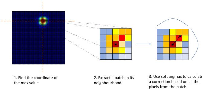
Figure 1: Proposed heatmap decoding. Given a predicted heatmap, (1) we find the location of the maximum, (2) and then crop around it a $k\times k$ patch. Finally, (3) we apply a softargmax on the patch and retrieve a correction applied to the location estimated at step (1).
图 1: 提出的热力图解码方法。给定预测的热力图,(1) 首先找到最大值的位置,(2) 然后在其周围裁剪一个 $k\times k$ 的补丁。最后,(3) 在该补丁上应用 softargmax 并获取对步骤 (1) 中估计位置的修正量。
3.3 Continuous Heatmap Decoding with Local Soft-argmax
3.3 基于局部软最大值 (Local Soft-argmax) 的连续热图解码
Currently, the typical landmark localization process from 2D heatmaps consists of finding the location of the pixel with the highest value [5]. This is typically followed by a heuristic correction with $0.25\mathrm{px}$ toward the location of the second highest neighboring pixel. The goal of this adjustment is to partially compensate for the effect induced by the quantization process: on one side by the heatmap generation process itself (as described in Section 3.2) and on other side, by the coarse nature of the predicted heatmap that uses the maximum value solely as the location of the point. We note that, despite the fact that the ground truth heatmaps are affected by quantization errors, generally, the networks learns to adjust, to some extent its predictions, making the later heuristic correction work well in practice.
目前,从二维热图中定位典型地标的过程通常包括寻找像素值最高的位置 [5]。随后通常会采用一个启发式修正,即向次高相邻像素的位置偏移 $0.25\mathrm{px}$。这一调整的目的是部分补偿量化过程带来的影响:一方面是热图生成过程本身(如第3.2节所述)导致的量化,另一方面是预测热图的粗糙性——仅将最大值作为点的位置。值得注意的是,尽管真实热图存在量化误差,但网络通常能在一定程度上学会调整其预测结果,使得后续的启发式修正在实践中效果良好。
Rather than using the above heuristic, we propose to predict the location of the keypoint by analyzing the pixels in its neighbourhood and exploiting the known targeted Gaussian distribution. For a given heatmap $\mathcal{H}{k}$ , we firstly find the coordinates corresponding to the maximum value $(\hat{y}{k}^{[\bar{1}]},\hat{y}{k}^{[2]})=\arg\operatorname*{max}\mathcal{H}{k}$ and then, around this location, we select a small square matrix $h_{k}$ of size $d\times d$ , where $\begin{array}{r}{l=\frac{d}{2}}\end{array}$ . Then, we predict an offset $(\Delta\hat{y}{k}^{[1]},\Delta\hat{y}_{k}^{[2]})$ by finding a soft continuous maximum value within the selected matrix, effectively retrieving a correction, using a local soft-argmax:
我们提出通过分析关键点邻域像素并利用已知目标高斯分布来预测其位置,而非采用上述启发式方法。对于给定热图 $\mathcal{H}{k}$,首先找到最大值对应坐标 $(\hat{y}{k}^{[\bar{1}]},\hat{y}{k}^{[2]})=\arg\operatorname*{max}\mathcal{H}{k}$,然后在该位置周围选取尺寸为 $d\times d$ 的小方阵 $h_{k}$(其中 $\begin{array}{r}{l=\frac{d}{2}}\end{array}$)。随后通过局部软最大值定位技术,在选定矩阵内寻找软连续最大值来预测偏移量 $(\Delta\hat{y}{k}^{[1]},\Delta\hat{y}_{k}^{[2]})$,从而获得修正量:
$$
\big(\Delta\hat{y}{k}^{[1]},\Delta\hat{y}{k}^{[2]}\big)=\sum_{m,n}\mathsf{s o f t m a x}(\tau h_{k})_{m,n}(m,n),
$$
$$
\big(\Delta\hat{y}{k}^{[1]},\Delta\hat{y}{k}^{[2]}\big)=\sum_{m,n}\mathsf{s o f t m a x}(\tau h_{k})_{m,n}(m,n),
$$
where $\tau$ is the temperature that controls the resulting probability map, and $(m,n)$ are the indices that iterate over the pixel coordinates of the heatmap $h_{k}$ . softmax is defined as:
其中 $\tau$ 是控制输出概率分布的温度参数,$(m,n)$ 是遍历热力图 $h_{k}$ 像素坐标的索引。softmax 定义为:
$$
\mathsf{s o f t m a x}(h){m,n}=\frac{e^{h_{m,n}}}{\sum_{m^{\prime},n^{\prime}}e^{h_{m^{\prime},n^{\prime}}}}
$$
$$
\mathsf{s o f t m a x}(h){m,n}=\frac{e^{h_{m,n}}}{\sum_{m^{\prime},n^{\prime}}e^{h_{m^{\prime},n^{\prime}}}}
$$
The final prediction is then obtained as: $(\hat{y}{k}^{[1]}+\Delta\hat{y}{k}^{[1]}-l,\hat{y}{k}^{[2]}+\Delta\hat{y}_{k}^{[2]}-l)$ . The 3 step process is illustrated in Fig. 1.
最终预测结果通过以下公式获得:$(\hat{y}{k}^{[1]}+\Delta\hat{y}{k}^{[1]}-l,\hat{y}{k}^{[2]}+\Delta\hat{y}_{k}^{[2]}-l)$。该三步流程如图 1 所示。
3.4 Siamese consistency training
3.4 孪生一致性训练
Largely, the face alignment training procedure has remained unchanged since the very first deep learning methods of [5, 65]. Herein, we propose to deviate from this paradigm adopting a Siamese-based training, where two different random augmentations of the same image are passed through the network, producing in the process a set of heatmaps. We then revert the transformation of each of these heatmaps and combine them via element-wise summation.
很大程度上,人脸对齐训练流程自最早的深度学习方法 [5, 65] 以来基本保持不变。本文中,我们提出采用基于孪生网络 (Siamese-based) 的训练范式,将同一张图像的两种不同随机增强版本输入网络,生成一组热力图 (heatmaps)。随后我们还原每张热力图的变换,并通过逐元素求和进行融合。
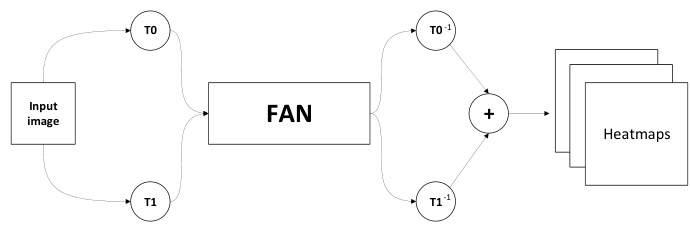
Figure 2: Siamese transformation-invariant training. T0 and T1 are two randomly sampled data augmentation transformations applied on the input image. After passing the augmented images through the network a set of heatmaps are produced. Finally, the transformations are reversed and the two outputs merged.
图 2: 孪生变换不变性训练。T0 和 T1 是输入图像上随机采样的两种数据增强变换。增强后的图像通过网络后生成一组热力图。最后,变换被逆转并将两个输出合并。
The advantages of this training process are twofold: Firstly, convolutional networks are not invariant under arbitrary affine transformations, and, as such, relatively small variances in the input space can result in large differences in the output. Therefore, by optimizing jointly and combining the two predictions we can improve the consistency of the predictions.
这种训练过程的优势有两点:首先,卷积网络在任意仿射变换下并不具有不变性,因此输入空间中相对较小的方差可能导致输出上的巨大差异。因此,通过联合优化并结合两个预测,我们可以提高预测的一致性。
Secondly, while previously the 2D Gaussians were always centered around an integer pixel location due to the quantization of the coordinates via rounding, the newly proposed heatmap generation can have the center in-between (i.e. on a sub-pixel). As such, to avoid small sub-pixel inconsistencies and misalignment introduced by the data augmentation process we adopt the above-mentioned Siamese based training. Our approach, depicted in Fig. 2, defines the output heatmaps $\hat{\mathcal{H}}$ as:
其次,由于之前通过坐标舍入量化,2D高斯分布始终以整数像素位置为中心,而新提出的热图生成方法可以将中心定位在像素之间(即亚像素位置)。为避免数据增强过程中引入的微小亚像素不一致和错位问题,我们采用了上述基于孪生网络的训练方法。如图 2 所示,我们的方法将输出热图 $\hat{\mathcal{H}}$ 定义为:
$$
\tilde{\mathcal{H}}=T_{0}^{-1}(\Phi(T_{0}(\mathbf{X}{i}),\theta))+T_{1}^{-1}(\Phi(T_{1}(\mathbf{X}_{i})),\theta),
$$
$$
\tilde{\mathcal{H}}=T_{0}^{-1}(\Phi(T_{0}(\mathbf{X}{i}),\theta))+T_{1}^{-1}(\Phi(T_{1}(\mathbf{X}_{i})),\theta),
$$
where $\Phi$ is the network for heatmap regression with parameters $\theta.T_{0}$ and $T_{1}$ are two random transformations applied on the input image $\mathbf{X}{i}$ and, $T_{0}^{-1}$ and $T_{1}^{-1}$ denote their inverse.
其中 $\Phi$ 是用于热图回归的网络,参数为 $\theta$。$T_{0}$ 和 $T_{1}$ 是应用于输入图像 $\mathbf{X}{i}$ 的两种随机变换,$T_{0}^{-1}$ 和 $T_{1}^{-1}$ 表示它们的逆变换。
4 Ablation studies
4 消融实验
4.1 Comparison with other landmarks localization losses
4.1 与其他地标定位损失函数的对比
Beyond comparisons with recently proposed methods for face alignment in Section 6 (e.g. [16, 24, 49]), herein we compare our approach against a few additional baselines.
除第6节中与近期提出的人脸对齐方法(如[16, 24, 49])的比较外,本文还将我们的方法与一些额外基线进行比较。
Heatmap prediction with coordinate correction: In DeepCut [33], for human pose estimation, the authors propose to add a coordinate refinement layer that predicts a $(\Delta\hat{y}{k}^{[1]},\Delta\hat{y}{k}^{[2]})$ displacement that is then added to the integer predictions generated by the heatmaps. To implement this, we added a global pooling operation followed by a fully connected layer and then trained it jointly using an $\ell_{2}$ loss. We attempted 2 different variants:where tisnstructed by measuring the heatmap encoding
带坐标修正的热图预测:在DeepCut [33]中,针对人体姿态估计任务,作者提出添加一个坐标细化层来预测位移量 $(\Delta\hat{y}{k}^{[1]},\Delta\hat{y}{k}^{[2]})$ ,该位移量会与热图生成的整数预测值相加。为实现这一机制,我们添加了全局池化操作和全连接层,并使用 $\ell_{2}$ 损失函数进行联合训练。我们尝试了两种不同变体:其中通过测量热图编码构建
errors and the other is dynamically constructed at runtime by measuring the error between the heatmap prediction and the ground truth. As Table 1 shows, these learned corrections offer minimal improvements on top of the standard heatmap regression loss and are noticeably worse than the accuracy scored by the proposed method. This shows that predicting sub-pixel errors using a second branch is less effective than constructing better heatmaps from the first place.
错误,另一个是在运行时通过测量热图预测与真实值之间的误差动态构建的。如表 1 所示,这些学习到的修正对标准热图回归损失的改进微乎其微,明显不如所提方法达到的精度。这表明使用第二个分支预测亚像素误差的效果不如从一开始就构建更好的热图。
Table 1: Comparison between various losses baselines on 300W test set.
表 1: 300W测试集上不同损失基线的对比
| 方法 | NMEbox |
|---|---|
| l2热图回归 | 2.32 |
| 坐标校正(静态gt) | 2.27 |
| 坐标校正(动态gt) | 2.30 |
| Globalsoft-argmax | 3.19 |
| Local soft-argmax(本文方法) | 2.04 |
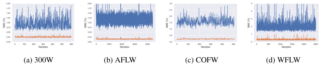
Figure 3: NME after encoding and then decoding of the ground truth heatmaps for various datasets using our proposed approach (orange) and the standard one [5] (blue). Notice that our approach significantly reduces the error rate across all samples from the datasets.
图 3: 采用我们提出的方法(橙色)和标准方法5对多个数据集的真实热图进行编码再解码后的NME。请注意,我们的方法显著降低了所有数据集样本的错误率。
Global soft-argmax: In [29], the authors propose to to predict the locations of the points of interest on the human body by estimating their position using a global soft-argmax as a differentiable alternative to taking the argmax. From a first glance this is akin to the idea proposed in this work: local soft-argmax. However, applying soft-argmax globally leads to semantically unstructured outputs [29] that hurt the performance. Even adding a Gaussian prior is insufficient for achieving high accuracy on face alignment. As the results from Table 1 conclusively show, our simple improvement, namely the proposed local soft-argmax is the key idea for obtaining highly accurate results.
全局 soft-argmax:在 [29] 中,作者提出通过全局 soft-argmax 作为可微分的 argmax 替代方案来预测人体关键点位置。初看这与本文提出的局部 soft-argmax 思路相似。但全局应用 soft-argmax 会导致语义结构缺失的输出 [29],从而影响性能。即使添加高斯先验也无法实现人脸对齐的高精度。如 表 1 结果明确所示,我们提出的局部 soft-argmax 这一简单改进才是获得高精度结果的关键。
4.2 Effect of method’s components
4.2 方法各组件的影响
Herein, we explore the impact of each our method’s component on the overall performance of the network. As the results from Table 2 show, starting from the baseline introduced in [5], the addition of the proposed heatmap encoding and decoding process significantly improves the accuracy. If we analyze this result in tandem with Fig. 3 it becomes apparent what is the source of these gains: In particular, Fig. 3 shows the heatmap encoding and decoding process of the baseline method [5] as well as of our method using directly the ground truth landmarks (i.e. these are not network’s predictions). As shown in Fig. 3, simply encoding and decoding the heatmaps corresponding to the ground truth alone induces high NME for [5]. While the training procedure is able to compensate this, these inaccuracies representations hinder the learning process. Furthermore, due to the sub-pixel errors introduced, the performance in the high accuracy regime of the cumulative error curve degrades.
本文探讨了方法中各组件对网络整体性能的影响。如表2所示,从文献[5]提出的基线方法出发,增加热图编码和解码过程后精度显著提升。结合图3分析可知性能提升的来源:图3对比展示了基线方法[5]与本方法(直接使用真实关键点,非网络预测)的热图编解码过程。如图所示,仅对真实值热图进行编解码就会导致[5]方法产生较高NME误差。虽然训练过程能够部分补偿这种误差,但这些不精确的表征仍会阻碍学习过程。此外,由于引入的亚像素误差,累积误差曲线在高精度区间的性能会出现下降。
Table 2: Effect of the proposed components on the WFLW dataset.
表 2: 所提组件在 WFLW 数据集上的效果
| 方法 | NMEic (%) |
|---|---|
| Baseline [5] | 4.20 |
| +proposedhm | 3.90 |
| + proposed hm (w/o 3.3) | 4.00 |
| +siamese training | 3.72 |
The rest of the gains are achieved by switching to the proposed Siamese training that reduces the discrepancies between multiple views of the same image while also reducing potential sub-pixel displacements that may occur between the image and the heatmaps.
其余增益通过切换至所提出的孪生训练 (Siamese training) 实现,该方法减少了同一图像多视角间的差异,同时降低了图像与热图之间可能出现的亚像素位移。
4.3 Local window size
4.3 局部窗口大小
In this section, we analyze the relation between the local soft-argmax window size and the model’s accuracy. As the results from Table 3 show, the optimal window has a size of
在本节中,我们分析了局部 soft-argmax 窗口大小与模型精度之间的关系。如表 3 所示,最佳窗口尺寸为
$5\times5\mathrm{px}$ , which corresponds to the size of the generated gaussian (i.e., most of the non-zero values will be contained within this window). Furthermore, as the window size increases the amount of noise and background pixels also increases and hence the accuracy decreases. The same value is used across all datasets. Note, that explicitly using the local window loss during training doesn’t improve the performance further which suggest that the pixel-wise loss alone is sufficient, if the encoding process is accurate.
5×5像素,这对应于生成的高斯窗口大小(即大部分非零值将包含在此窗口内)。此外,随着窗口尺寸增大,噪声和背景像素的数量也会增加,从而导致精度下降。所有数据集均采用相同值。需注意的是,在训练期间显式使用局部窗口损失并不会进一步提升性能,这表明只要编码过程准确,仅像素级损失就已足够。
5 Experimental setup
5 实验设置
Datasets: We preformed extensive evaluations to quantify the effectiveness of the proposed method. We trained and/or tested our method on the following datasets: 300W [38] (constructed in [38] using images from LFPW [1], AFW [64], HELEN [25] and iBUG [39]), 300W-LP [65],
数据集:我们进行了大量评估以量化所提方法的有效性。在以下数据集上训练和/或测试了我们的方法:300W [38](使用来自LFPW [1]、AFW [64]、HELEN [25]和iBUG [39]的图像构建于[38]中)、300W-LP [65]
Table 3: Effect of window size on the 300W test set.
表 3: 窗口大小对 300W 测试集的影响
| none | 3×3 5×5 | 7×7 | |
|---|---|---|---|
| NMEbox | 2.21 | 2.06 | 2.04 2.07 |
Menpo [58], COFW-29 [7], COFW-68 [17], AFLW [22], WFLW [50] and 300VW [41]. For a detailed description of each dataset see supplementary material.
Menpo [58]、COFW-29 [7]、COFW-68 [17]、AFLW [22]、WFLW [50] 和 300VW [41]。各数据集的详细说明见补充材料。
Metrics: Depending on the evaluation protocol of each dataset we used one or more of the following metrics:
指标:根据每个数据集的评估协议,我们使用以下一个或多个指标:
Normalized Mean Error (NME) that measures the point-to-point normalized Euclidean distance. Depending on the testing protocol, the NME type will vary. In this paper, we distinguish between the following types: $d_{i c}$ – computed as the inter-occular distance [38], $d_{b o x}$ – computed as the geometric mean of the ground truth bounding box [5] $d=\sqrt{(\boldsymbol{w}{b b o x}}$ · $h_{b b o x})$ , and finally $d_{d i a g}$ – defined as the diagonal of the bounding box.
归一化平均误差 (NME) 用于测量点对点归一化欧氏距离。根据测试协议不同,NME 类型会有所变化。本文区分了以下类型:$d_{i c}$ —— 以眼间距离计算 [38],$d_{b o x}$ —— 以真实标注框的几何平均数计算 [5] $d=\sqrt{(\boldsymbol{w}{b b o x}}$ · $h_{b b o x})$,最后是 $d_{d i a g}$ —— 定义为标注框的对角线长度。
Area Under the Curve(AUC): The AUC is computed by measuring the area under the curve up to a given user defined cut-off threshold of the cumulative error curve.
曲线下面积 (AUC): AUC的计算方法是测量累积误差曲线在用户定义的截止阈值下的曲线下面积。
Failure Rate (FR): The failure rate is defined as the percentage of images the NME of which is bigger than a given (large) threshold.
失败率 (FR): 失败率定义为归一化最大误差 (NME) 超过给定 (较大) 阈值的图像百分比。
5.1 Training details
5.1 训练细节
For training the models used throughout this paper we largely followed the common best practices from literature. Mainly, during training we applied the following augmentation techniques: Random rotation (between $\pm30^{o}$ ), image flipping and color(0.6, 1.4) and scale jittering (between 0.85 and 1.15). The models where trained for 50 epochs using a step scheduler that dropped the learning rate at epoch 25 and 40 starting from a starting learning rate of 0.0001. Finally, we used Adam [21] for optimization. The predicted heatmaps were at a resolution of $64\times64\mathrm{px}$ , i.e. $4\times$ smaller than the input images which were resized to $256\times$ 256 pixels with the face size being approximately equal to $220\times220\mathrm{px}$ . The network was optimized using an $\ell_{2}$ pixel-wise loss. For the heatmap decoding process, the temperature of the soft-argmax $\tau$ was set to 10 for all datasets, however slightly higher values perform similarly. Values that are too small or high would ignore and respectively overly emphasise the pixels found around the coordinates of the max. All the experiments were implemented using PyTorch [32] and Kornia [35].
在训练本文所用模型时,我们主要遵循文献中的常见最佳实践。训练过程中主要应用了以下数据增强技术:随机旋转(范围 $\pm30^{o}$)、图像翻转、色彩调整(0.6-1.4倍)以及尺度抖动(0.85-1.15倍)。模型训练50个epoch,采用分步学习率调度器,初始学习率为0.0001,在第25和40个epoch时降低学习率。优化器选用Adam [21]。预测热图分辨率为 $64\times64\mathrm{px}$(即比输入图像缩小 $4\times$ 倍),输入图像统一调整为 $256\times256$ 像素,面部区域尺寸约为 $220\times220\mathrm{px}$。网络优化采用 $\ell_{2}$ 逐像素损失函数。热图解码过程中,soft-argmax的温度参数 $\tau$ 在所有数据集均设为10(略高值表现相近),过小或过大的值会分别忽略或过度强调最大值坐标周围的像素。所有实验均通过PyTorch [32]和Kornia [35]实现。
Network architecture: All models trained throughout this work, unless otherwise specified, follow a 2-stack Hourglass based architecture with a width of 256 channels, operating at a resolution of $256\times256\mathrm{px}$ as introduced in [5]. Inside the hourglass, the features are rescaled down-to $4\times4\mathrm{px}$ and then upsampled back, with skip connection linking features found at the same resolution. The network is constructed used the building block from [4] as in [5]. For more details regarding the network structure see [5, 31].
网络架构:除非另有说明,本研究中训练的所有模型均采用基于双栈Hourglass的架构,宽度为256通道,工作分辨率为$256\times256\mathrm{px}$,如[5]所述。在Hourglass内部,特征被下采样至$4\times4\mathrm{px}$后再进行上采样,并通过跳跃连接(skip connection)链接同分辨率特征。该网络使用[4]提出的构建模块搭建,具体方法见[5]。更多网络结构细节请参阅[5, 31]。
6 Comparison against state-of-the-art
6 与最先进技术的对比
Herein, we compare against the current state-of-the-art face alignment methods across a plethora of datasets. Throughout this section the best result is marked in table with bold and red while the second best with bold and blue color. The important finding of this section is by means of two simple improvements: (a) improving the heatmap encoding and decoding process and, (b) including the Siamese training, we managed to obtain results which are significantly better than all recent prior work, setting in this way a new state-of-the-art.
在此,我们与当前最先进的人脸对齐方法在多个数据集上进行了比较。本节中,最佳结果在表格中以加粗红色标记,次佳结果以加粗蓝色标记。本部分的重要发现在于通过两项简单改进:(a) 优化热图编码解码过程,(b) 引入连体训练 (Siamese training),我们取得了显著优于近期所有相关工作的成果,从而确立了新的技术标杆。
Comparison on WFLW: On WFLW, and following their evaluation protocol, we report results in terms of $\mathrm{NME}{i c}$ , $\mathrm{AUC}{i c}^{10}$ and $\mathrm{FR}{i c}^{10}$ . As the results from Table 10 show, our method improves the previous best results of [24] by more than $0.5%$ for $\mathrm{NME}{i c}$ and $5%$ in terms of $\mathrm{AUC}_{i c}^{10}$ almost halving the error rate. This shows that our method offers improvements in the high accuracy regime while also reducing the overall failure ratio for difficult images.
WFLW上的对比:在WFLW数据集上,遵循其评估协议,我们以$\mathrm{NME}{i c}$、$\mathrm{AUC}{i c}^{10}$和$\mathrm{FR}{i c}^{10}$为指标报告结果。如表10所示,我们的方法将[24]的最佳结果在$\mathrm{NME}{i c}$上提升了超过$0.5%$,在$\mathrm{AUC}_{i c}^{10}$上提升了$5%$,几乎将错误率减半。这表明我们的方法在高精度区域实现了改进,同时降低了困难图像的整体失败率。
Comparison on AFLW: Following [24], we report results in terms of $\mathrm{NME}{d i a g}$ , $\mathrm{NME}{b o x}$ and $\mathrm{AUC}_{b o x}^{7}$ . As the results from Table 11 show, we improve across all metrics on top of the current best result even on this nearly saturated dataset.
AFLW对比实验:参照[24],我们采用$\mathrm{NME}{diag}$、$\mathrm{NME}{box}$和$\mathrm{AUC}_{box}^{7}$作为评估指标。如表11所示,即使在这个近乎饱和的数据集上,我们的方法仍在所有指标上超越了当前最佳结果。
Table 4: Results on WFLW (a) and $300\mathbf{W}$ (b) datasets.
(a) Comparison against the state-of-the-art on (b) Comparison against state-of-the-art on the WFLW in terms of . ${\mathrm{NME}}{i n t e r-o c u l a r}$ , $\mathrm{AUC}{i c}^{10}$ and 300W Common, Challenge and Full datasets (i.e. and $\mathrm{FR}_{i c}^{10}$ Split II) in terms of NMEinter−occular
表 4: WFLW (a) 和 $300\mathbf{W}$ (b) 数据集上的结果。
| 方法 | NMEic(%) | AUC!0 | FR10 (%) | Common | Challenge | Full | |
|---|---|---|---|---|---|---|---|
| Wing [16] | 5.11 | 0.554 | 6.00 | Teacher[11] | 2.91 | 5.91 | 3.49 |
| MHHN [47] | 4.77 | DU-Net [46] | 2.97 | 5.53 | 3.47 | ||
| DeCaFa [10] | 4.62 | 0.563 | 4.84 | DeCaFa [10] | 2.93 | 5.26 | 3.39 |
| AVS [34] | 4.39 | 0.591 | 4.08 | HR-Net [43] | 2.87 | 5.15 | 3.32 |
| AWing [49] | 4.36 | 0.572 | 2.84 | HG-HSLE [66] | 2.85 | 5.03 | 3.28 |
| LUVLi [24] | 4.37 | 0.577 | 3.12 | Awing[49] | 2.72 | 4.52 | 3.07 |
| GCN [26] | 4.21 | 0.589 | 3.04 | LUVLi [24] | 2.76 | 5.16 | 3.23 |
| Ours | 3.72 | 0.631 | 1.55 | Ours | 2.61 | 4.13 | 2.94 |
(a) 在 WFLW 数据集上关于 ${\mathrm{NME}}{inter-ocular}$、$\mathrm{AUC}{ic}^{10}$ 和 $\mathrm{FR}_{ic}^{10}$ 的先进方法对比 (b) 在 300W Common、Challenge 和 Full 数据集 (即 Split II) 上关于 NMEinter−occular 的先进方法对比
Comparison on 300W: Following the protocol described in [38] and [5], we report results in terms of ${\mathrm{NME}{i n t e r-o c c u l a r}}$ for Split I and of AUC7b and $\mathrm{NME}_{b o x}$ for split II. Note that due to the overlap between the splits we train two separate models, one on the data from the first split and another on the data from the other split evaluating the models accordingly. Following [5, 24] the model evaluated on the test set was pretrained on 300W
300W数据集对比:按照[38]和[5]中描述的协议,我们分别报告Split I的${\mathrm{NME}{inter-ocular}}$指标,以及Split II的AUC7b和$\mathrm{NME}_{box}}$指标。需要注意的是,由于数据划分存在重叠,我们训练了两个独立模型:一个基于第一划分数据训练,另一个基于另一划分数据训练,并相应评估模型性能。依照[5,24]的方法,测试集评估的模型均在300W数据集上进行了预训练。
Table 5: Comparison on COFW-29. Results for other methods taken from [43].
| 方法 | NMEic (%) | FR10 (%) |
|---|---|---|
| Wing [16] | 5.07 | 3.16 |
| LAB(w/B)[51] | 3.92 | 0.39 |
| HR-Net [43] | 3.45 | 0.19 |
| 本文方法 | 3.02 | 0.0 |
表 5: COFW-29数据集上的对比结果。其他方法的结果取自[43]。
BULAT ET AL.: SUBPIXEL HEATMAP REGRES. FOR FACIAL LANDMARK LOCALIZATION 9
BULAT ET AL.: 基于亚像素热图回归的面部关键点定位 9
| 方法 | NMEdiag Full | NMEdiag Frontal | NMEbox Full | Full |
|---|---|---|---|---|
| SAN [12] | 1.91 | 1.85 | 4.04 | 54.0 |
| DSNR [30] | 1.85 | 1.62 | ||
| LAB (w/o B) [51] | 1.85 | 1.62 | ||
| HR-Net [43] | 1.57 | 1.46 | ||
| Wing [16] | 3.56 | 53.5 | ||
| KDN [9] | 2.80 | 60.3 | ||
| LUVLi [24] | 1.39 | 1.19 | 2.28 | 68.0 |
| MHHN [47] | 1.38 | 1.19 | ||
| Ours | 1.31 | 1.12 | 2.14 | 70.0 |
Table 6: Comparison against the state-of-the-art on the AFLW-19 dataset.
Table 7: Comparison against the state-of-the-art on the 300W Test (i.e. Split I), Menpo 2D Frontal and COFW-68 datasets in terms of $\mathrm{NME}{b o x}$ and $\mathrm{AUC}_{b o x}^{7}$ .
表 6: AFLW-19 数据集上的先进方法对比
| 方法 | NMEbox | AUCbox | ||||
|---|---|---|---|---|---|---|
| 300-W | Menpo | COFW-68 | 300-W | Menpo | COFW-68 | |
| SAN [12] | 2.86 | 2.95 | 3.50 | 59.7 | 61.9 | 51.9 |
| FAN [5] | 2.32 | 2.16 | 2.95 | 66.5 | 69.0 | 57.5 |
| Softlabel[9] | 2.32 | 2.27 | 2.92 | 66.6 | 67.4 | 57.9 |
| KDN [9] | 2.21 | 2.01 | 2.73 | 68.3 | 71.1 | 60.1 |
| LUVLi [24] | 2.10 | 2.04 | 2.57 | 70.2 | 71.9 | 63.4 |
| Ours | 2.04 | 1.95 | 2.47 | 71.1 | 73.0 | 64.9 |
表 7: 在 300W Test (即 Split I)、Menpo 2D Frontal 和 COFW-68 数据集上关于 $\mathrm{NME}{box}$ 和 $\mathrm{AUC}_{box}^{7}$ 的先进方法对比。
LP dataset. As the results from Table 12 show, our approach offers consistent improvements across both subsets (i.e. Common and Challenge), with particularly higher gains on the later. Similar results can be observer in Table 7 for Split II.
LP数据集。如表 12 所示,我们的方法在两个子集(即Common和Challenge)上都表现出一致的改进,后者提升尤为显著。表 7 中Split II的实验结果也呈现相似趋势。
Comparison on COFW: On the COFW dataset we evaluate on both the 29-point (see Table 13) and 68-point configuration (see Table 7) in terms of $\mathrm{NME}{i c}(%)$ and $\mathrm{FR}{i c}^{10}$ for the 29-point configuration and $\mathrm{NME}{b o x}$ , $\mathrm{AUC}_{b o x}^{7}$ for the other one. As the results from Tables 7 and 13 show, our method sets a new state-of-the-art, reducing the failure rate to 0.0.
COFW数据集对比:在COFW数据集上,我们分别评估了29点(见表13)和68点(见表7)配置。对于29点配置,采用 $\mathrm{NME}{i c}(%)$ 和 $\mathrm{FR}{i c}^{10}$ 指标;对于68点配置,则使用 $\mathrm{NME}{b o x}$ 和 $\mathrm{AUC}_{b o x}^{7}$ 指标。如表7和表13所示,我们的方法实现了新的最优性能,将失败率降至0.0。
Comparison on Menpo: Following [24] we evaluate on the frontal sub-set of the Menpo dataset. As Table 7 shows, our method sets a new state-of-the-art result.
Menpo数据集对比:按照[24]的方法,我们在Menpo数据集的正面子集上进行评估。如表7所示,我们的方法取得了新的最先进成果。
Comparison on 300VW: Unlike the previous datasets that focus on face alignment for static images, 300VW is a video face tracking dataset. Following [41], we report results in terms of $\mathrm{AUC}_{i c}@0.08$ on the most challenging partition of the test set (C). As the results from Table 8 show, despite not exploiting any temporal information and running our method on a frame-by-frame basis, we set a new state-of-the-art, outperforming previous tracking methods trained such as [40] and [18]. Similar results can be observed when evaluating on all 68 points in Table 9.
300VW数据集对比:与之前专注于静态图像人脸对齐的数据集不同,300VW是一个视频人脸追踪数据集。按照[41]的方法,我们在测试集最具挑战性的分区(C)上以$\mathrm{AUC}_{i c}@0.08$指标报告结果。如表8所示,尽管未利用任何时序信息且逐帧运行我们的方法,我们仍创造了新的最优性能,超越了[40]和[18]等经过训练的追踪方法。如表9所示,当评估所有68个关键点时也能观察到类似结果。
| 方法 | 我们的方法 | DGM [18] | CPM+SRB+PAM [13] | iCCR [40] | [57] | [54] |
|---|---|---|---|---|---|---|
| AUCic@0.08 | 60.10 | 59.38 | 59.39 | 51.41 | 49.96 | 48.65 |
Table 8: Comparison against the state-of-the-art on the 300-VW dataset – category C, in terms of $\mathrm{AUC}_{i c}@0.08$ evaluated on the 49 inner points.
表 8: 在300-VW数据集类别C上的最新技术对比 (基于49个内部点评估的 $\mathrm{AUC}_{i c}@0.08$ 指标)
| 方法 | 我们的方法 | FHR+STA [44] | TSTN [27] | TCDCN [60] | CFSS [62] |
|---|---|---|---|---|---|
| NMEic | 5.84 | 5.98 | 12.80 | 15.0 | 13.70 |
Table 9: Comparison against the state-of-the-art on the 300-VW dataset – category C (i.e., scenario 3), in terms of $\mathrm{NME}_{i c}$ evaluated on all 68 points. Results for other methods taken from [44].
表 9: 在 300-VW 数据集 - 类别 C (即场景 3) 上与其他先进方法的对比, 以所有 68 个点评估的 $\mathrm{NME}_{i c}$ 为指标。其他方法的结果取自 [44]。

Figure 4: Qualitative results. Landmarks shown in white are produced by our method, while the ones in red by the state-of-the-art approach of [5]. Thanks to the proposed heatmap encoding and decoding, our method is able to provide much more accurate results. Best viewed zoomed in, in electronic format.
图 4: 定性对比结果。白色标记点为本方法生成结果,红色标记点为文献[5]当前最优方法所生成。得益于提出的热图编码解码机制,本方法能提供更精确的结果。建议放大电子版查看细节。

Figure 5: Examples of failure cases. Most of the failure cases include combinations of low resolution images with extreme poses (1st and 4th image), perspective distortions (5th image) or overlapping faces (3rd image).
图 5: 失败案例示例。大多数失败案例包含低分辨率图像与极端姿态(第1和第4张图)、透视畸变(第5张图)或人脸重叠(第3张图)的组合情况。
7 Conclusions
7 结论
We presented simple yet effective improvements to standard methods for face alignment which are shown to dramatically increase the accuracy on all benchmarks considered without introducing sophisticated changes to existing architectures and loss functions. The proposed improvements concern a fairly unexplored topic in face alignment that of the heatmap encoding and decoding process. We showed that the proposed continuous heatmap regression provides a significantly improved approach for the encoding/decoding process. Moreover, we showed that further improvements can be obtained by considering a simple Siamese training procedure that enforces output spatial consistency of geometrically transformed images. We hope that these improvements will be incorporated in future research while it is not unlikely that many existing methods will also benefit by them.
我们针对标准人脸对齐方法提出了简单而有效的改进方案,这些改进在不改变现有架构和损失函数复杂度的前提下,显著提升了所有测试基准的准确率。所提出的改进聚焦于人脸对齐领域中研究较少的课题——热图编码与解码过程。我们证明了提出的连续热图回归方法为编码/解码过程提供了显著优化的解决方案。此外,通过采用简单的连体训练策略来增强几何变换图像输出结果的空间一致性,还能获得进一步的性能提升。希望这些改进方案能被未来研究采纳,同时现有诸多方法也很可能从中受益。
References
参考文献
[1] Peter N Belhumeur, David W Jacobs, David J Kriegman, and Neeraj Kumar. Localizing parts of faces using a consensus of exemplars. TPAMI, 2013.
[1] Peter N Belhumeur, David W Jacobs, David J Kriegman 和 Neeraj Kumar. 基于范例共识的人脸局部定位方法. TPAMI, 2013.
[2] Adrian Bulat and Georgios Tzi miro poul os. Convolutional aggregation of local evidence for large pose face alignment. In BMVC, 2016.
[2] Adrian Bulat 和 Georgios Tzimiropoulos. 大姿态人脸对齐的局部证据卷积聚合. 见: BMVC, 2016.
[15] Zhen-Hua Feng, Josef Kittler, William Christmas, Patrik Huber, and Xiao-Jun Wu. Dynamic attention-controlled cascaded shape regression exploiting training data augmentation and fuzzy-set sample weighting. In Proceedings of the IEEE conference on computer vision and pattern recognition, pages 2481–2490, 2017.
[15] Zhen-Hua Feng, Josef Kittler, William Christmas, Patrik Huber, and Xiao-Jun Wu. 基于训练数据增强与模糊集样本加权的动态注意力控制级联形状回归。In Proceedings of the IEEE conference on computer vision and pattern recognition, pages 2481–2490, 2017.
[16] Zhen-Hua Feng, Josef Kittler, Muhammad Awais, Patrik Huber, and Xiao-Jun Wu. Wing loss for robust facial landmark local is ation with convolutional neural networks. In Proceedings of the IEEE Conference on Computer Vision and Pattern Recognition, pages 2235–2245, 2018.
[16] Zhen-Hua Feng, Josef Kittler, Muhammad Awais, Patrik Huber, 和 Xiao-Jun Wu。基于卷积神经网络的 Wing 损失鲁棒人脸关键点定位。载于《IEEE 计算机视觉与模式识别会议论文集》,第 2235–2245 页,2018 年。
[28] Rosanne Liu, Joel Lehman, Piero Molino, Felipe Petroski Such, Eric Frank, Alex Sergeev, and Jason Yosinski. An intriguing failing of convolutional neural networks and the coordconv solution. arXiv preprint arXiv:1807.03247, 2018.
[28] Rosanne Liu, Joel Lehman, Piero Molino, Felipe Petroski Such, Eric Frank, Alex Sergeev, Jason Yosinski. 卷积神经网络的一个有趣缺陷及CoordConv解决方案. arXiv预印本 arXiv:1807.03247, 2018.
[29] Diogo C Luvizon, David Picard, and Hedi Tabia. 2d/3d pose estimation and action recognition using multitask deep learning. In Proceedings of the IEEE Conference on Computer Vision and Pattern Recognition, pages 5137–5146, 2018.
[29] Diogo C Luvizon, David Picard 和 Hedi Tabia. 基于多任务深度学习的2D/3D姿态估计与动作识别. 载于《IEEE计算机视觉与模式识别会议论文集》, 第5137-5146页, 2018.
[39] Christos Sagonas, Georgios Tzi miro poul os, Stefanos Zafeiriou, and Maja Pantic. A semi-automatic methodology for facial landmark annotation. In CVPR, 2013.
[39] Christos Sagonas, Georgios Tzimiropoulos, Stefanos Zafeiriou 和 Maja Pantic. 一种半自动化的面部关键点标注方法. 发表于 CVPR, 2013.
[40] Enrique Sánchez-Lozano, Georgios Tzi miro poul os, Brais Martinez, Fernando De la Torre, and Michel Valstar. A functional regression approach to facial landmark tracking. IEEE transactions on pattern analysis and machine intelligence, 40(9):2037–2050, 2017.
[40] Enrique Sánchez-Lozano, Georgios Tzimiropoulos, Brais Martinez, Fernando De la Torre, Michel Valstar. 面部特征点跟踪的功能回归方法. IEEE模式分析与机器智能汇刊, 40(9):2037–2050, 2017.
[52] Wenyan Wu and Shuo Yang. Leveraging intra and inter-dataset variations for robust face alignment. In Proceedings of the IEEE conference on computer vision and pattern recognition workshops, pages 150–159, 2017.
[52] Wenyan Wu 和 Shuo Yang. 利用数据集内和数据集间变化实现鲁棒人脸对齐. 见: IEEE计算机视觉与模式识别研讨会论文集, 第150-159页, 2017.
[53] Bin Xiao, Haiping Wu, and Yichen Wei. Simple baselines for human pose estimation and tracking. In Proceedings of the European conference on computer vision (ECCV), pages 466–481, 2018.
[53] Bin Xiao, Haiping Wu, and Yichen Wei. 人体姿态估计与跟踪的简单基线方法. In Proceedings of the European conference on computer vision (ECCV), pages 466–481, 2018.
[66] Xu Zou, Sheng Zhong, Luxin Yan, Xiangyun Zhao, Jiahuan Zhou, and Ying Wu. Learning robust facial landmark detection via hierarchical structured ensemble. In Proceedings of the IEEE/CVF International Conference on Computer Vision, pages 141–150, 2019.
[66] Xu Zou, Sheng Zhong, Luxin Yan, Xiangyun Zhao, Jiahuan Zhou, and Ying Wu. 通过分层结构化集成学习鲁棒的面部关键点检测. In Proceedings of the IEEE/CVF International Conference on Computer Vision, pages 141–150, 2019.
A Datasets
A 数据集
In this paper we conducton experiments on the following datasets:
在本文中,我们在以下数据集上进行了实验:
300W: 300W [38] is a 2D face alignment dataset constructed by concatenating and then manually re-anotating with 68 points the images from LFPW [1], AFW [64], HELEN [25] and iBUG [39]. There are two commonly used train/test splits. Split I: uses 3837 images for training and 600 for testing and Split II that uses 3148 facial images for training and 689 for testing. The later testset comprises of two subsets: common and challenge. Most of the images present in the dataset contain faces found in frontal or near-frontal poses.
300W: 300W [38] 是一个通过合并LFPW [1]、AFW [64]、HELEN [25]和iBUG [39]数据集图像并手动重新标注68个关键点构建的2D人脸对齐数据集。该数据集包含两种常用的训练/测试划分方式:划分I使用3837张图像训练、600张测试;划分II采用3148张面部图像训练、689张测试。后者的测试集包含两个子集:常规集和挑战集。数据集中大多数图像为正面或接近正面的人脸姿态。
300W-LP: 300W-LP [65] is a synthetically generated dataset formed by warping into large poses the images from the 300W dataset. This dataset contains 61,125 pre-warped images and is used for training alone.
300W-LP: 300W-LP [65] 是通过对300W数据集图像进行大姿态扭曲生成的合成数据集,包含61,125张预扭曲图像且仅用于训练。
Menpo: Menpo [58] is a 2D face alignment dataset that annotates the images using 2 different configurations depending on the pose of the faces. The near frontal facial images are annotated using the same 68 points configuration used for 300W, while the rest using 39 points. In this work, we trained and evaluated on the 68-point configuration.
Menpo: Menpo [58] 是一个2D人脸对齐数据集,根据面部姿态采用两种不同配置进行图像标注。近正面人脸图像使用与300W相同的68点配置标注,其余则采用39点配置。本工作中,我们基于68点配置进行训练和评估。
COFW: The Caltech Occluded Faces in the Wild (COFW) [7] dataset contains 1,345 training and 507 testing facial images captured in real world scenarios and annotated using 29 points. The images were later on re-annotated in [17] using the same 68-point configuration as in 300W.
COFW: Caltech Occluded Faces in the Wild (COFW) [7] 数据集包含1,345张训练图像和507张测试图像,这些图像是在真实场景中拍摄的面部图像,并使用29个关键点进行标注。后来在[17]中,这些图像被重新标注,采用了与300W相同的68个关键点配置。
AFLW: The Annotated Facial Landmarks in the Wild (AFLW) [22] dataset consists of 20,000 training images and 4386 testing images, out of which 1314 are part of the Frontal subset. All images are annotated using a 19 point configuration.
AFLW: 野外标注面部关键点 (Annotated Facial Landmarks in the Wild, AFLW) [22] 数据集包含 20,000 张训练图像和 4386 张测试图像,其中 1314 张属于正面子集。所有图像均采用 19 点配置进行标注。
WFLW: Wider Facial Landmarks in-the-wild (WFLW) [50] consists of 10,000 images, out of which 7,500 are used for training while the rest are reserved for testing. All images are annotated using a 98 point configuration. In addition to landmarks, the dataset is also annotated with a set of attributes.
WFLW: Wider Facial Landmarks in-the-wild (WFLW) [50] 包含10,000张图像,其中7,500张用于训练,其余用于测试。所有图像均采用98个关键点标注方案。除关键点外,该数据集还标注了若干属性。
300VW: 300VW [41] is a large scale video face alignment dataset consisting of 218,594 frames distributed across 114 videos, out of which 50 are reserved for training while the rest for testing. The test set is further split into 3 different categories (A, B an C) with C being the most challenging one. We note that due to the semi-supervised annotation procedure some images have erroneous labels.
300VW: 300VW [41] 是一个大规模视频人脸对齐数据集,包含分布在114个视频中的218,594帧图像,其中50个视频用于训练,其余用于测试。测试集进一步分为3个不同类别 (A、B和C),其中C类最具挑战性。我们注意到,由于半监督标注流程,部分图像存在错误标签。
B Metrics
B 指标
其中 ${\bf y}{k}$ 表示第 $k$ 个人脸的真实标注坐标,$\hat{\bf y}{\bf k}$ 是对应的预测坐标,$d_{t y p e}$ 为归一化距离类型。
the points are normalized. $\mathbf{v}_{k}$ is a visibility binary vector, with values 1 at the landmarks where the ground truth is provided and 0 everywhere else.
点被归一化。$\mathbf{v}_{k}$ 是一个可见性二元向量,在地标点处提供真实值时取值为1,其余位置为0。
Depending on the testing protocol, the NME type (i.e. how it’s computed and defined) will vary. In this paper, we distinguish between the following types: $d_{i c}$ – computed as the inter-occular distance [38], $d_{b o x}$ – computed as the geometric mean of the ground truth bounding box [5] $d=\sqrt{\left(w_{b b o x}\cdot h_{b b o x}\right)}$ , and finally $d_{d i a g}$ – defined as the diagonal of the bounding box.
根据测试协议的不同,归一化误差 (NME) 的计算和定义方式也会有所差异。本文区分了以下几种类型:$d_{i c}$——以瞳距计算 [38],$d_{b o x}$——以标注框几何平均数计算 [5] $d=\sqrt{\left(w_{b b o x}\cdot h_{b b o x}\right)}$,以及$d_{d i a g}$——定义为标注框对角线长度。
Area Under the Curve(AUC): The AUC is computed by measuring the area under the curve up to a given user defined cut-off threshold of the cumulative error curve. Compared with NME that simple takes the average, this metric is less prone to outliers.
曲线下面积 (AUC): AUC通过计算累积误差曲线在用户定义的截止阈值下的曲线下面积来衡量。与简单取平均值的NME相比,该指标对异常值更不敏感。
Failure Rate (FR): The failure rate is defined as the percentage of images the NME of which is bigger than a given (large) threshold.
失败率 (FR):失败率定义为归一化匹配误差 (NME) 超过给定(较大)阈值的图像百分比。
C Additional comparisons with state-of-the-art
C 与当前最优方案的补充对比
In addition to the comparisons reported in the main paper here in we show how our method performs against an additional set of methods (Tables 10, 11, 12, 12, 13).
除了主论文中报告的对比之外,我们在此展示了我们的方法相对于另外一组方法的性能表现 (表 10, 11, 12, 12, 13)。
$\mathrm{AUC}{i c}^{10}$ 0a:n d $\mathrm{FR}_{i c}^{1\bar{0}}$ .arison against the state-of-the-art on WFLW in terms of NMEinter−ocular,
$\mathrm{AUC}{i c}^{10}$ 0a:n d $\mathrm{FR}_{i c}^{1\bar{0}}$ .arison against the state-of-the-art on WFLW in terms of NMEinter−ocular,
| 方法 | NMEic(%) | AUC!O | FRI0 (%) |
|---|---|---|---|
| ESR [8] | 11.13 | 0.277 | 35.24 |
| SDM [56] | 10.29 | 0.300 | 29.40 |
| CFSS [62] | 9.07 | 0.366 | 20.56 |
| DVLN [52] | 6.08 | 0.456 | 10.84 |
| LAB (w/B) [51] | 5.27 | 0.532 | 7.56 |
| Wing [16] | 5.11 | 0.554 | 6.00 |
| MHHN [47] | 4.77 | - | - |
| DeCaFa [10] | 4.62 | 0.563 | 4.84 |
| AVS [34] | 4.39 | 0.591 | 4.08 |
| AWing [49] | 4.36 | 0.572 | 2.84 |
| LUVLi [24] | 4.37 | 0.577 | 3.12 |
| GCN [26] | 4.21 | 0.589 | 3.04 |
| Ours | 3.72 | 0.631 | 1.55 |
Table 11: Comparison against the state-of-the-art on the AFLW-19 dataset.
表 11: AFLW-19数据集上与其他先进方法的对比
| 方法 | NMEdiag Full | NMEdiag Frontal | NMEbox Full | AUC? box Full |
|---|---|---|---|---|
| RCPR [7] | 3.73 | 2.87 | ||
| CFSS [62] | 3.92 | 2.68 | ||
| CCL [63] | 2.72 | 2.17 | ||
| DAC-CSR [15] | 2.27 | 1.81 | ||
| LLL [36] | 1.97 | |||
| CPM+SRB [13] | 2.14 | |||
| SAN [12] | 1.91 | 1.85 | 4.04 | 54.0 |
| DSNR [30] | 1.85 | 1.62 | ||
| LAB (w/o B) [51] | 1.85 | 1.62 | ||
| HR-Net [43] | 1.57 | 1.46 | ||
| Wing [16] | 3.56 | 53.5 | ||
| KDN [9] | 2.80 | 60.3 | ||
| LUVLi [24] | 1.39 | 1.19 | 2.28 | 68.0 |
| MHHN [47] | 1.38 | 1.19 | ||
| Ours | 1.31 | 1.12 | 2.14 | 70.0 |
Table 12: Comparison against state-of-the-art on the 300W Common, Challenge and Full datasets (i.e. Split II).
表 12: 在 300W Common、Challenge 和 Full 数据集 (即 Split II) 上与最先进方法的对比
| 方法 | NMEinter-occular |
|---|---|
| Common | |
| ODN [61] | 3.56 |
| CPM+SRB [13] | 3.28 |
| SAN [12] | 3.34 |
| AVS [34] | 3.21 |
| DAN [23] | 3.19 |
| LAB (w/B) [51] | 2.98 |
| Teacher [11] | 2.91 |
| DU-Net [46] | 2.97 |
| DeCaFa [10] | 2.93 |
| HR-Net [43] | 2.87 |
| HG-HSLE [66] | 2.85 |
| Awing [49] | 2.72 |
| LUVLi [24] | 2.76 |
| Ours | 2.61 |
Table 13: Comparison against the state-of-the-art on the COFW-29 dataset.
表 13: COFW-29数据集上的最新方法对比。
| 方法 | NMEic(%) | FRi0 (%) |
|---|---|---|
| Human | 5.60 | |
| ESR [8] | 11.20 | 36.0 |
| RCPR [7] | 8.50 | 20.00 |
| HPM | 7.59 | 13.00 |
| CCR [14] | 7.03 | 10.90 |
| DRDA [59] | 6.49 | 6.00 |
| RAR [55] | 6.03 | 4.14 |
| DAC-CSR [15] | 6.03 | 4.73 |
| LAB (w/o B) [51] | 5.58 | 2.76 |
| Wing [16] | 5.07 | 3.16 |
| MHHN [47] | 4.95 | 1.78 |
| LAB (w/B) [51] | 3.92 | 0.39 |
| HR-Net [43] | 3.45 | 0.19 |
| Ours | 3.02 | 0.0 |