Temporal Cycle-Consistency Learning
时序周期一致性学习
Debidatta Dwibedi 1, Yusuf Aytar 2, Jonathan Tompson 1, Pierre Sermanet 1, and Andrew Zisserman 2 1 Google Brain 2 DeepMind {debidatta, yusufaytar, tompson, sermanet, zisserman}@google.com
Debidatta Dwibedi 1, Yusuf Aytar 2, Jonathan Tompson 1, Pierre Sermanet 1, and Andrew Zisserman 2
1 Google Brain
2 DeepMind
{debidatta, yusufaytar, tompson, sermanet, zisserman}@google.com
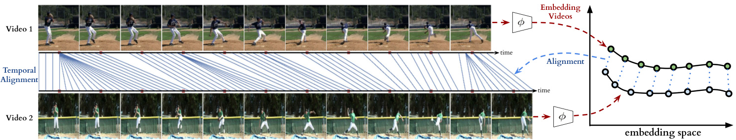
Figure 1: We present a self-supervised representation learning technique called temporal cycle consistency (TCC) learning. It is inspired by the temporal video alignment problem, which refers to the task of finding correspondences across multiple videos despite many factors of variation. The learned representations are useful for fine-grained temporal understanding in videos. Additionally, we can now align multiple videos by simply finding nearest-neighbor frames in the embedding space.
图 1: 我们提出了一种称为时序循环一致性 (TCC) 学习的自监督表征学习方法。该方法受时序视频对齐问题的启发,该问题指在存在多种变化因素的情况下寻找多个视频间对应关系的任务。学习到的表征可用于视频中的细粒度时序理解。此外,我们现在只需在嵌入空间中找到最近邻帧即可对齐多个视频。
Abstract
摘要
We introduce a self-supervised representation learning method based on the task of temporal alignment between videos. The method trains a network using temporal cycleconsistency (TCC), a differentiable cycle-consistency loss that can be used to find correspondences across time in multiple videos. The resulting per-frame embeddings can be used to align videos by simply matching frames using nearest-neighbors in the learned embedding space.
我们提出了一种基于视频间时序对齐任务的自监督表征学习方法。该方法使用时序循环一致性 (TCC) 训练网络,这是一种可微分的循环一致性损失函数,可用于在多个视频中寻找跨时间对应关系。通过学习得到的逐帧嵌入表示,只需在嵌入空间中使用最近邻匹配帧,即可实现视频对齐。
To evaluate the power of the embeddings, we densely label the Pouring and Penn Action video datasets for action phases. We show that (i) the learned embeddings enable few-shot classification of these action phases, significantly reducing the supervised training requirements; and (ii) TCC is complementary to other methods of selfsupervised learning in videos, such as Shuffle and Learn and Time-Contrastive Networks. The embeddings are also used for a number of applications based on alignment (dense temporal correspondence) between video pairs, including transfer of metadata of synchronized modalities between videos (sounds, temporal semantic labels), synchronized playback of multiple videos, and anomaly detection. Project webpage: https://sites.google. com/view/temporal-cycle-consistency.
为了评估嵌入(embedding)的效果,我们对Pouring和Penn Action视频数据集进行了动作阶段的密集标注。研究表明:(i) 学习到的嵌入可实现对这些动作阶段的少样本分类,显著降低监督训练需求;(ii) TCC与视频自监督学习的其他方法(如Shuffle and Learn和Time-Contrastive Networks)具有互补性。这些嵌入还可用于基于视频对之间对齐(密集时间对应关系)的多种应用,包括视频间同步模态元数据(声音、时间语义标签)的迁移、多视频同步播放以及异常检测。项目网页:https://sites.google.com/view/temporal-cycle-consistency。
1. Introduction
1. 引言
The world presents us with abundant examples of sequential processes. A plant growing from a seedling to a tree, the daily routine of getting up, going to work and coming back home, or a person pouring themselves a glass of water – are all examples of events that happen in a particular order. Videos capturing such processes not only contain information about the causal nature of these events, but also provide us with a valuable signal – the possibility of temporal correspondences lurking across multiple instances of the same process. For example, during pouring, one could be reaching for a teapot, a bottle of wine, or a glass of water to pour from. Key moments such as the first touch to the container or the container being lifted from the ground are common to all pouring sequences. These correspondences, which exist in spite of many varying factors like visual changes in viewpoint, scale, container style, the speed of the event, etc., could serve as the link between raw video sequences and high-level temporal abstractions (e.g. phases of actions). In this work we present evidence that suggests the very act of looking for correspondences in sequential data enables the learning of rich and useful representations, particularly suited for fine-grained temporal understanding of videos.
世界为我们提供了丰富的序列过程实例。从幼苗长成大树、每日起床工作回家的生活作息,到人们为自己倒水的动作,都是以特定顺序发生的事件范例。记录这类过程的视频不仅蕴含了事件因果本质的信息,更提供了一种宝贵信号——相同过程多个实例间可能潜藏着时序对应关系。例如倒水动作中,人们可能伸手去拿茶壶、葡萄酒瓶或水杯作为容器。首次触碰容器或将容器从桌面举起等关键瞬间,是所有倒水序列共有的特征。尽管存在视角变化、尺度差异、容器样式、动作速度等诸多变量,这些跨越视觉差异的对应关系,仍能成为原始视频序列与高层时序抽象(如动作阶段)之间的桥梁。本研究通过实证表明:在序列数据中寻找对应关系这一行为本身,就能促使模型学习到丰富且实用的表征,尤其适用于视频的细粒度时序理解。
Temporal reasoning in videos, understanding multiple stages of a process and causal relations between them, is a relatively less studied problem compared to recognizing action categories [10, 42]. Learning representations that can differentiate between states of objects as an action proceeds is critical for perceiving and acting in the world. It would be desirable for a robot tasked with learning to pour drinks to understand each intermediate state of the world as it proceeds with performing the task. Although videos are a rich source of sequential data essential to understanding such state changes, their true potential remains largely untapped. One hindrance in the fine-grained temporal understanding of videos can be an excessive dependence on pure supervised learning methods that require per-frame annotations. It is not only difficult to get every frame labeled in a video because of the manual effort involved, but also it is not entirely clear what are the exhaustive set of labels that need to be collected for fine-grained understanding of videos. Alternatively, we explore self-supervised learning of correspondences between videos across time. We show that the emerging features have strong temporal reasoning capacity, which is demonstrated through tasks such as action phase classification and tracking the progress of an ac- tion.
视频中的时序推理(理解一个过程的多个阶段及其因果关系)与识别动作类别相比[10,42],是一个研究相对较少的问题。学习能够区分动作进行中物体状态变化的表征,对于感知和行动至关重要。例如,一个学习倒饮料的机器人需要理解任务执行过程中每个中间状态。尽管视频是理解这类状态变化的重要序列数据来源,但其真正潜力尚未被充分挖掘。阻碍视频细粒度时序理解的一个因素可能是对纯监督学习方法的过度依赖,这类方法需要逐帧标注。不仅因为人工标注成本高而难以获取视频中每一帧的标签,而且对于视频细粒度理解需要收集哪些完整标签集也并不完全明确。为此,我们探索了跨时间视频对应关系的自监督学习方法,证明所提取的特征具备强大的时序推理能力,这通过动作阶段分类和动作进度跟踪等任务得到验证。
When frame-by-frame alignment (i.e. supervision) is available, learning correspondences reduces to learning a common embedding space from pairs of aligned frames (e.g. CCA [3, 4] and ranking loss [35]). However, for most of the real world sequences such frame-by-frame alignment does not exist naturally. One option would be to artificially obtain aligned sequences by recording the same event through multiple cameras [30, 35, 37]. Such data collection methods might find it difficult to capture all the variations present naturally in videos in the wild. On the other hand, our self-supervised objective does not need explicit correspondences to align different sequences. It can align significant variations within an action category (e.g. pouring liquids, or baseball pitch). Interestingly, the embeddings that emerge from learning the alignment prove to be useful for fine-grained temporal understanding of videos. More specifically, we learn an embedding space that maximizes one-to-one mappings (i.e. cycle-consistent points) across pairs of video sequences within an action category. In order to do that, we introduce two differentiable versions of cycle consistency computation which can be optimized by conventional gradient-based optimization methods. Further details of the method will be explained in section 3.
当存在逐帧对齐(即监督)时,学习对应关系简化为从对齐的帧对中学习共同的嵌入空间(例如CCA [3, 4] 和排序损失 [35])。然而,对于大多数现实世界序列,这种逐帧对齐并不自然存在。一种选择是通过多台摄像机记录同一事件来人工获取对齐序列 [30, 35, 37]。此类数据收集方法可能难以捕捉自然视频中存在的所有变化。另一方面,我们的自监督目标不需要显式对应关系来对齐不同序列。它可以对齐动作类别内的显著变化(例如倒液体或棒球投球)。有趣的是,通过学习对齐产生的嵌入被证明对视频的细粒度时间理解非常有用。更具体地说,我们学习了一个嵌入空间,该空间在动作类别内的视频序列对之间最大化一对一映射(即循环一致点)。为此,我们引入了两种可微分的循环一致性计算版本,可以通过传统的基于梯度的优化方法进行优化。该方法的更多细节将在第3节中解释。
The main contribution of this paper is a new selfsupervised training method, referred to as temporal cycle consistency (TCC) learning, that learns representations by aligning video sequences of the same action. We compare TCC representations against features from existing selfsupervised video representation methods [27, 35] and supervised learning, for the tasks of action phase classification and continuous progress tracking of an action. Our ap- proach provides significant performance boosts when there is a lack of labeled data. We also collect per-frame annotations of Penn Action [52] and Pouring [35] datasets that we will release publicly to facilitate evaluation of fine-grained video understanding tasks.
本文的主要贡献是提出了一种新的自监督训练方法,称为时序循环一致性 (TCC) 学习,该方法通过对齐相同动作的视频序列来学习表征。我们将 TCC 表征与现有自监督视频表征方法 [27, 35] 和监督学习的特征进行了比较,用于动作阶段分类和动作连续进度跟踪任务。在缺乏标注数据的情况下,我们的方法显著提升了性能。我们还收集了 Penn Action [52] 和 Pouring [35] 数据集的逐帧标注,并将公开释放以促进细粒度视频理解任务的评估。
2. Related Work
2. 相关工作
Cycle consistency. Validating good matches by cycling between two or more samples is a commonly used technique in computer vision. It has been applied successfully for tasks like co-segmentation [43, 44], structure from motion [49, 51], and image matching [54, 55, 56]. For in- stance, FlowWeb [54] optimizes globally-consistent dense correspondences using the cycle consistent flow fields between all pairs of images in a collection, whereas Zhou et al. [56] approaches a similar task by formulating it as a low-rank matrix recovery problem and solves it through fast alternating minimization. These methods learn robust dense correspondences on top of fixed feature representations (e.g. SIFT, deep features, etc.) by enforcing cycle consistency and/or spatial constraints between the images. Our method differs from these approaches in that TCC is a self-supervised representation learning method which learns embedding spaces that are optimized to give good correspondences. Furthermore we address a temporal correspondence problem rather than a spatial one. Zhou et al. [55] learn to align multiple images using the supervision from 3D guided cycle-consistency by leveraging the initial correspondences that are available between multiple renderings of a 3D model, whereas we don’t assume any given correspondences. Another way of using cyclic relations is to directly learn bi-directional transformation functions between multiple spaces such as CycleGANs [57] for learning image transformations, and CyCADA [21] for domain adaptation. Unlike these approaches we don’t have multiple domains, and we can’t learn transformation functions between all pairs of sequences. Instead we learn a joint embedding space in which the Euclidean distance defines the mapping across the frames of multiple sequences. Similar to us, Aytar et al. [7] applies cycle-consistency between temporal sequences, however they use it as a validation tool for hyper-parameter optimization of learned representations for the end goal of imitation learning. Unlike our approach, their cycle-consistency measure is non-differentiable and hence can’t be directly used for representation learning.
循环一致性 (Cycle consistency)。通过在两个或多个样本之间进行循环验证良好匹配是计算机视觉中常用的技术。该方法已成功应用于协同分割 [43, 44]、运动恢复结构 [49, 51] 和图像匹配 [54, 55, 56] 等任务。例如,FlowWeb [54] 通过优化图像集中所有图像对之间的循环一致流场来获得全局一致的密集对应关系,而 Zhou 等人 [56] 则将该任务表述为低秩矩阵恢复问题,并通过快速交替最小化求解。这些方法通过在固定特征表示 (如 SIFT、深度特征等) 基础上强制执行循环一致性和/或空间约束,学习鲁棒的密集对应关系。我们的方法 TCC 与这些方法的不同之处在于,它是一种自监督表示学习方法,通过学习优化的嵌入空间来获得良好的对应关系。此外,我们解决的是时间对应问题而非空间对应问题。Zhou 等人 [55] 利用 3D 模型多视角渲染之间的初始对应关系,通过 3D 引导的循环一致性监督来学习对齐多幅图像,而我们不需要任何给定的对应关系。另一种利用循环关系的方法是直接学习多个空间之间的双向变换函数,例如用于图像变换的 CycleGANs [57] 和用于域适应的 CyCADA [21]。与这些方法不同,我们没有多个域,也无法学习所有序列对之间的变换函数。相反,我们学习一个联合嵌入空间,其中欧氏距离定义了跨多个序列帧的映射。与我们类似,Aytar 等人 [7] 在时间序列之间应用循环一致性,但他们将其作为超参数优化的验证工具,最终目标是模仿学习。与我们的方法不同,他们的循环一致性度量是不可微的,因此不能直接用于表示学习。
Video alignment. When we have synchronization information (e.g. multiple cameras recording the same event) then learning a mapping between multiple video sequences can be accomplished by using existing methods such as Canonical Correlation Analysis (CCA) [3, 4], ranking [35] or match-classification [6] objectives. For instance TCN [35] and circulant temporal encoding [30] align multiple views of the same event, whereas Sigurdsson et al.[37] learns to align first and third person videos. Although we have a similar objective, these methods are not suitable for our task as we cannot assume any given correspondences between different videos.
视频对齐。当我们拥有同步信息(例如多个摄像机录制同一事件)时,可以通过使用现有方法(如典型相关分析 (CCA) [3, 4]、排序 [35] 或匹配分类 [6] 目标)来学习多个视频序列之间的映射。例如,TCN [35] 和循环时间编码 [30] 对齐同一事件的多视角视频,而 Sigurdsson 等人 [37] 则学习对齐第一人称和第三人称视频。尽管我们有类似的目标,但这些方法并不适用于我们的任务,因为我们无法假设不同视频之间存在任何给定的对应关系。
Action localization and parsing. As action recognition is quite popular in the computer vision community, many studies [17, 38, 46, 50, 53] explore efficient deep architectures for action recognition and localization in videos. Past work has also explored parsing of fine-grained actions in videos [24, 25, 29] while some others [13, 33, 34, 36] discover sub-activities without explicit supervision of temporal boundaries. [20] learns a supervised regression model with voting to predict the completion of an action, and [2] discovers key events in an un super iv sed manner using a weak association between videos and text instructions. However all these methods heavily rely on existing deep image [19, 39] or spatio-temporal [45] features, whereas we learn our representation from scratch using raw video sequences. Soft nearest neighbours. The differentiable or soft formulation for nearest-neighbors is a commonly known method [18]. This formulation has recently found application in metric learning for few-shot learning [28, 31, 40]. We also make use of soft nearest neighbor formulation as a component in our differentiable cycle-consistency computation.
动作定位与解析。动作识别在计算机视觉领域相当流行,许多研究[17, 38, 46, 50, 53]探索了视频中动作识别与定位的高效深度架构。以往工作还研究了视频中细粒度动作的解析[24, 25, 29],而另一些研究[13, 33, 34, 36]则在无显式时间边界监督的情况下发现子活动。[20]通过带投票的监督回归模型预测动作完成度,[2]则利用视频与文本指令间的弱关联以无监督方式发现关键事件。然而这些方法都严重依赖现有深度图像[19, 39]或时空特征[45],而我们的表征直接从原始视频序列学习。软最近邻。可微分或软化的最近邻公式是广为人知的方法[18]。该公式最近被应用于少样本学习的度量学习[28, 31, 40]。我们也将软最近邻公式作为可微分循环一致性计算的组成部分。
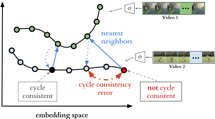
Figure 2: Cycle-consistent representation learning. We show two example video sequences encoded in an example embedding space. If we use nearest neighbors for matching, one point (shown in black) is cycling back to itself while another one (shown in red) is not. Our target is to learn an embedding space where maximum number of points can cycle back to themselves. We achieve it by minimizing the cycle consistency error (shown in red dotted line) for each point in every pair of sequences.
图 2: 循环一致性表示学习。我们展示了在示例嵌入空间中编码的两个视频序列。若采用最近邻匹配,一个点(黑色所示)能循环回到自身,而另一个点(红色所示)则不能。我们的目标是学习一个能使最多点实现自我循环的嵌入空间,通过最小化每对序列中每个点的循环一致性误差(红色虚线所示)来实现这一目标。
Self-supervised representations. There has been significant progress in learning from images and videos without requiring class or temporal segmentation labels. Instead of labels, self-supervised learning methods use signals such as temporal order [16, 27], consistency across viewpoints and/or temporal neighbors [35], classifying arbitrary temporal segments [22], temporal distance classification within or across modalities [7], spatial permutation of patches [5, 14], visual similarity [32] or a combination of such signals [15]. While most of these approaches optimize each sample independently, TCC jointly optimizes over two sequences at a time, potentially capturing more variations in the embedding space. Additionally, we show that TCC yields best results when combined with some of the unsupervised losses above.
自监督表示。在不依赖类别或时序分割标签的情况下,从图像和视频中学习已取得显著进展。自监督学习方法通过以下信号替代标签:时序顺序 [16, 27]、跨视角和/或时序邻域的一致性 [35]、对任意时序片段的分类 [22]、模态内或跨模态的时序距离分类 [7]、图像块的空间排列 [5, 14]、视觉相似性 [32] 或上述信号的组合 [15]。虽然大多数方法独立优化每个样本,但 TCC 同时优化两个序列,从而能在嵌入空间中捕捉更多变化。此外,我们证明 TCC 与上述某些无监督损失函数结合时效果最佳。
3. Cycle Consistent Representation Learning
3. 循环一致性表示学习
The core contribution of this work is a self-supervised approach to learn an embedding space where two similar video sequences can be aligned temporally. More specifically, we intend to maximize the number of points that can be mapped one-to-one between two sequences by using the minimum distance in the learned embedding space. We can achieve such an objective by maximizing the number of cycle-consistent frames between two sequences (see Figure 2). However, cycle-consistency computation is typically not a differentiable procedure. In order to facilitate learning such an embedding space using back-propagation, we introduce two differentiable versions of the cycle-consistency loss, which we describe in detail below.
本工作的核心贡献在于提出了一种自监督学习方法,用于构建一个能将两个相似视频序列在时间轴上对齐的嵌入空间。具体而言,我们旨在通过学习到的嵌入空间中的最小距离,最大化两个序列间可建立一对一映射的点位数量。这一目标可通过最大化两个序列间循环一致帧(cycle-consistent frames)的数量来实现(见图 2)。然而,循环一致性计算通常不具备可微性。为了通过反向传播学习此类嵌入空间,我们引入了两种可微循环一致性损失函数变体,具体描述如下。
Given any frame $s_{i}$ in a sequence ${\cal S}={s_{1},s_{2},...,s_{N}}$ , the embedding is computed as $u_{i}=\phi(s_{i};\theta)$ , where $\phi$ is the neural network encoder parameterized by $\theta$ . For the following sections, assume we are given two video sequences $S$ and $T$ , with lengths $N$ and $M$ , respectively. Their embeddings are computed as $U={u_{1},u_{2},...,u_{N}}$ and $V=$ ${v_{1},v_{2},...,v_{M}}$ such that $u_{i}=\phi(s_{i};\theta)$ and $v_{i}=\phi(t_{i};\theta)$ .
给定序列 ${\cal S}={s_{1},s_{2},...,s_{N}}$ 中的任意帧 $s_{i}$,其嵌入计算为 $u_{i}=\phi(s_{i};\theta)$,其中 $\phi$ 是由参数 $\theta$ 参数化的神经网络编码器。在后续章节中,假设给定两个视频序列 $S$ 和 $T$,长度分别为 $N$ 和 $M$。它们的嵌入计算为 $U={u_{1},u_{2},...,u_{N}}$ 和 $V=$ ${v_{1},v_{2},...,v_{M}}$,满足 $u_{i}=\phi(s_{i};\theta)$ 和 $v_{i}=\phi(t_{i};\theta)$。
3.1. Cycle-consistency
3.1. 循环一致性
In order to check if a point $u_{i}\in U$ is cycle consistent, we first determine its nearest neighbor, $v_{j}=\mathrm{arg}\mathrm{min}{v\in V}|u_{i}-$ $v||$ . We then repeat the process to find the nearest neighbor of $v_{j}$ in $U$ , i.e. . The point $u_{i}$ is cycle-consistent if and only if $i=k$ , in other words if the point $u_{i}$ cycles back to itself. Figure 2 provides positive and negative examples of cycle consistent points in an embedding space. We can learn a good embedding space by maximizing the number of cycle-consistent points for any pair of sequences. However that would require a differentiable version of cycle-consistency measure, two of which we introduce below.
为了检查点 $u_{i}\in U$ 是否满足循环一致性,我们首先确定其最近邻 $v_{j}=\mathrm{arg}\mathrm{min}{v\in V}|u_{i}-$ $v||$。接着重复该过程,在 $U$ 中寻找 $v_{j}$ 的最近邻,即 当且仅当 $i=k$ 时(换言之,若点 $u_{i}$ 能循环映射回自身),该点满足循环一致性。图 2 展示了嵌入空间中循环一致性点的正例与反例。通过最大化任意序列对的循环一致点数量,我们可以学习到良好的嵌入空间。但这需要可微分的循环一致性度量方法,下文将介绍其中两种。
3.2. Cycle-back Classification
3.2. 回环分类
We first compute the soft nearest neighbor $\widetilde{v}$ of $u_{i}$ in $V$ , then figure out the nearest neighbor of $\widetilde{v}$ ba cek in $U$ . We consider each frame in the first sequence $U$ to be a separate class and our task of checking for cycle-consistency reduces to classification of the nearest neighbor correctly. The logits are calculated using the distances between $\widetilde{v}$ and any $u_{k}\in$ $U$ , and the ground truth label $y$ are all zero se except for the $i^{t h}$ index which is set to 1.
我们首先计算$u_{i}$在$V$中的软最近邻$\widetilde{v}$,然后找出$\widetilde{v}$在$U$中的最近邻。我们将第一个序列$U$中的每一帧视为一个独立类别,此时循环一致性检查任务转化为对最近邻的正确分类问题。logits通过计算$\widetilde{v}$与任意$u_{k}\in U$之间的距离获得,真实标签$y$除第$i^{th}$位设为1外其余均为0。
For the selected point $u_{i}$ , we use the softmax function to define its soft nearest neighbor $\widetilde{v}$ as:
对于选定的点 $u_{i}$,我们使用 softmax 函数定义其软最近邻 $\widetilde{v}$ 为:
$$
\widetilde{v}=\sum_{j}^{M}\alpha_{j}v_{j},\quad w h e r e\quad\alpha_{j}=\frac{e^{-||u_{i}-v_{j}||^{2}}}{\sum_{k}^{M}e^{-||u_{i}-v_{k}||^{2}}}
$$
$$
\widetilde{v}=\sum_{j}^{M}\alpha_{j}v_{j},\quad 其中\quad\alpha_{j}=\frac{e^{-||u_{i}-v_{j}||^{2}}}{\sum_{k}^{M}e^{-||u_{i}-v_{k}||^{2}}}
$$
and $\alpha$ is the the similarity distribution which signifies the proximity between $u_{i}$ and each $v_{j}\in V$ . And then we solve the $N$ class (i.e. number of frames in $U$ ) classification problem where the logits are $x_{k}=-||\widetilde{v}-u_{k}||^{2}$ and the predicted labels are $\hat{y}=s o f t m a x(x)$ . Finalely we optimize the cross-
且 $\alpha$ 是表示 $u_{i}$ 与每个 $v_{j}\in V$ 之间接近度的相似性分布。接着我们求解 $N$ 类(即 $U$ 中的帧数)分类问题,其中逻辑值为 $x_{k}=-||\widetilde{v}-u_{k}||^{2}$,预测标签为 $\hat{y}=softmax(x)$。最后我们优化交叉-
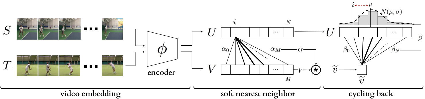
Figure 3: Temporal cycle consistency. The embedding sequences $U$ and $V$ are obtained by encoding video sequences $S$ and $T$ with the encoder network $\phi$ , respectively. For the selected point $u_{i}$ in $U$ , soft nearest neighbor computation and cycling back to $U$ again is demonstrated visually. Finally the normalized distance between the index $i$ and cycling back distribution $N(\mu,\sigma^{2})$ (which is fitted to $\beta$ ) is minimized.
图 3: 时序循环一致性。嵌入序列 $U$ 和 $V$ 分别通过编码器网络 $\phi$ 对视频序列 $S$ 和 $T$ 进行编码获得。对于 $U$ 中选定的点 $u_{i}$,以可视化方式展示了软最近邻计算及再次循环回 $U$ 的过程。最终最小化索引 $i$ 与循环回分布 $N(\mu,\sigma^{2})$ (拟合至 $\beta$) 之间的归一化距离。
entropy loss as follows:
熵损失如下:
$$
L_{c b c}=-\sum_{j}^{N}y_{j}\log(\hat{y}_{j})
$$
$$
L_{c b c}=-\sum_{j}^{N}y_{j}\log(\hat{y}_{j})
$$
3.3. Cycle-back Regression
3.3. 循环回归 (Cycle-back Regression)
Although cycle-back classification defines a differentiable cycle-consistency loss function, it has no notion of how close or far in time the point to which we cycled back is. We want to penalize the model less if we are able to cycle back to closer neighbors as opposed to the other frames that are farther away in time. In order to incorporate temporal proximity in our loss, we introduce cycle-back regression. A visual description of the entire process is shown in Figure 3. Similar to the previous method first we compute the soft nearest neighbor $\widetilde{v}$ of $u_{i}$ in $V$ . Then we compute the similarity vector $\beta$ tha te defines the proximity between $\widetilde{v}$ and each $u_{k}\in U$ as:
虽然循环分类定义了一个可微的循环一致性损失函数,但它没有考虑循环返回的时间点距离远近。我们希望当模型能循环返回时间上更接近的相邻帧时,给予较小惩罚,反之则给予较大惩罚。为了在损失函数中引入时间邻近性,我们提出了循环回归方法。整个过程的可视化描述见图3。与前文方法类似,首先我们计算$u_{i}$在$V$中的软最近邻$\widetilde{v}$,然后计算相似度向量$\beta$,该向量通过以下方式定义$\widetilde{v}$与每个$u_{k}\in U$之间的邻近关系:
$$
\beta_{k}=\frac{e^{-||\widetilde{v}-u_{k}||^{2}}}{\sum_{j}^{N}e^{-||\widetilde{v}-u_{j}||^{2}}}
$$
$$
\beta_{k}=\frac{e^{-||\widetilde{v}-u_{k}||^{2}}}{\sum_{j}^{N}e^{-||\widetilde{v}-u_{j}||^{2}}}
$$
Note that $\beta$ is a discrete distribution of similarities over time and we expect it to show a peaky behavior around the $i^{t h}$ index in time. Therefore, we impose a Gaussian prior on $\beta$ by minimizing the normalized squared distance $\frac{|i-\mu|^{2}}{\sigma^{2}}$ as our objective. We enforce $\beta$ to be more peaky around $i$ by applying additional variance regular iz ation. We define our final objective as:
注意到 $\beta$ 是一个随时间变化的相似性离散分布,我们期望它在时间维度上的第 $i^{t h}$ 个索引附近呈现峰值特性。因此,我们通过最小化归一化平方距离 $\frac{|i-\mu|^{2}}{\sigma^{2}}$ 作为目标函数,对 $\beta$ 施加高斯先验。为了增强 $\beta$ 在 $i$ 附近的峰值特性,我们额外应用了方差正则化。最终目标函数定义为:
$$
L_{c b r}=\frac{|i-\mu|^{2}}{\sigma^{2}}+\lambda\log(\sigma)
$$
$$
L_{c b r}=\frac{|i-\mu|^{2}}{\sigma^{2}}+\lambda\log(\sigma)
$$
where $\begin{array}{r}{\mu=\sum_{k}^{N}\beta_{k}k}\end{array}$ and $\begin{array}{r}{\sigma^{2}=\sum_{k}^{N}\beta_{k}(k-\mu)^{2}}\end{array}$ , and $\lambda$ is the reg u lari z ation weight. No te that we minimize the log of variance as using just the variance is more prone to numerical instabilities. All these formulations are differentiable and can conveniently be optimized with conventional back-propagation.
其中 $\begin{array}{r}{\mu=\sum_{k}^{N}\beta_{k}k}\end{array}$ 和 $\begin{array}{r}{\sigma^{2}=\sum_{k}^{N}\beta_{k}*(k-\mu)^{2}}\end{array}$ ,$\lambda$ 为正则化权重。需要注意的是,我们最小化方差的对数,因为直接使用方差更容易出现数值不稳定的情况。所有这些公式都是可微分的,可以通过常规的反向传播方便地进行优化。
Table 1: Architecture of the embedding network.
| 操作 | 输出尺寸 | 参数 |
|---|---|---|
| 时序堆叠3D卷积 | k×14×14×512 | 堆叠k个上下文帧 [3×3×3,512]×2 |
| 时空池化 | 512 | 全局3D最大池化 |
| 全连接层 | 512 | [512]×2 |
| 线性投影 | 128 | 128 |
表 1: 嵌入网络架构。
3.4. Implementation details
3.4. 实现细节
Training Procedure. Our self-supervised representation is learned by minimizing the cycle-consistency loss for all the pair of sequences in the training set. Given a sequence pair, their frames are embedded using the encoder network and we optimize cycle consistency losses for randomly selected frames within each sequence until convergence. We used Tensorflow [1] for all our experiments.
训练过程。我们的自监督表征是通过最小化训练集中所有序列对的循环一致性损失来学习的。给定一个序列对,我们使用编码器网络嵌入其帧,并针对每个序列中随机选择的帧优化循环一致性损失,直至收敛。所有实验均使用 Tensorflow [1] 实现。
Encoding Network. All the frames in a given video sequence are resized to $224\times224$ . When using ImageNet pretrained features, we use ResNet-50 [19] architecture to extract features from the output of Conv4c layer. The size of the extracted convolutional features are $14\times14\times1024$ . Because of the size of the datasets, when training from scratch we use a smaller model along the lines of VGG-M [11]. This network takes input at the same resolution as ResNet50 but is only 7 layers deep. The convolutional features produced by this base network are of the size $14\times14\times512$ . These features are provided as input to our embedder network (presented in Table 1). We stack the features of any given frame and its $k$ context frames along the dimension of time. This is followed by 3D convolutions for aggregating temporal information. We reduce the dimensionality by using 3D max-pooling followed by two fully connected layers. Finally, we use a linear projection to get a 128- dimensional embedding for each frame. More details of the architecture are presented in the supplementary material.
编码网络。给定视频序列中的所有帧都被调整为 $224\times224$ 大小。使用ImageNet预训练特征时,我们采用ResNet-50 [19]架构从Conv4c层输出中提取特征,提取的卷积特征尺寸为 $14\times14\times1024$。由于数据集规模限制,在从头训练时我们使用类似VGG-M [11]的轻量模型,该网络输入分辨率与ResNet50相同但仅含7层,基础网络生成的卷积特征尺寸为 $14\times14\times512$。这些特征将作为嵌入网络(结构见表1)的输入。我们将目标帧及其 $k$ 个上下文帧的特征沿时间维度堆叠,随后通过3D卷积聚合时序信息,并使用3D最大池化降维后接两个全连接层,最终通过线性投影得到每帧的128维嵌入向量。架构详情见补充材料。
4. Datasets and Evaluation
4. 数据集与评估
We validate the usefulness of our representation learning technique on two datasets: (i) Pouring [35]; and ( ii)
我们在两个数据集上验证了表征学习技术的有效性:(i) Pouring [35];以及(ii)
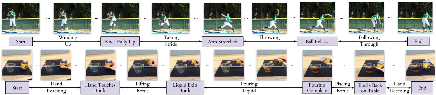
Figure 4: Example labels for the actions ‘Baseball Pitch’ (top row) and ‘Pouring’ (bottom row). The key events are shown in boxes below the frame (e.g. ‘Hand touches bottle’), and each frame in between two key events has a phase label (e.g. ‘Lifting bottle’).
图 4: "棒球投球"(上排)和"倒水"(下排)动作的示例标签。关键事件显示在帧下方的方框中(例如"手触碰瓶子"),两个关键事件之间的每一帧都有阶段标签(例如"举起瓶子")。
Penn Action [52]. These datasets both contain videos of humans performing actions, and provide us with collections of videos where dense alignment can be performed. While Pouring focuses more on the objects being interacted with, Penn Action focuses on humans doing sports or exercise.
Penn Action [52]。这两个数据集都包含人类执行动作的视频,为我们提供了可进行密集对齐的视频集合。Pouring更侧重于被交互的物体,而Penn Action则聚焦于人类进行体育运动或锻炼的场景。
Annotations. For evaluation purposes, we add two types of labels to the video frames of these datasets: key events and phases. Densely labeling each frame in a video is a difficult and time-consuming task. Labelling only key events both reduces the number of frames that need to be annotated, and also reduces the ambiguity of the task (and thus the disagreement between annotators). For example, annotators agree more about the frame when the golf club hits the ball (a key event) than when the golf club is at a certain angle. The phase is the period between two key events, and all frames in the period have the same phase label. It is similar to tasks proposed in [9, 12, 23]. Examples of key events and phases are shown in Figure 4, and Table 2 gives the complete list for all the actions we consider.
标注。出于评估目的,我们为这些数据集的视频帧添加了两种类型的标签:关键事件和阶段。对视频中的每一帧进行密集标注是一项困难且耗时的任务。仅标注关键事件既减少了需要标注的帧数,也降低了任务的模糊性(从而减少了标注者之间的分歧)。例如,标注者对于高尔夫球杆击中球的帧(关键事件)比对于高尔夫球杆处于某一角度的帧更容易达成一致。阶段是两个关键事件之间的时间段,该时间段内的所有帧都具有相同的阶段标签。这与[9, 12, 23]中提出的任务类似。关键事件和阶段的示例如图4所示,表2给出了我们所考虑的所有动作的完整列表。
We use all the real videos from the Pouring dataset, and all but two action categories in Penn Action. We do not use Strumming guitar and Jumping rope because it is difficult to define unambiguous key events for these. We use the train/val splits of the original datasets [35, 52]. We will publicly release these new annotations.
我们使用了Pouring数据集中的所有真实视频,以及Penn Action中除两个动作类别外的所有内容。我们没有使用弹吉他(Strumming guitar)和跳绳(Jumping rope)这两个类别,因为很难为它们定义明确的关键事件。我们采用了原始数据集的训练/验证划分方式[35, 52]。这些新标注将公开释放。
4.1. Evaluation
4.1. 评估
We use three evaluation measures computed on the validation set. These metrics evaluate the model on fine-grained temporal understanding of a given action. Note, the networks are first trained on the training set and then frozen. SVM class if i ers and linear regressors are trained on the features from the networks, with no additional fine-tuning of the networks. For all measures a higher score implies a better model.
我们在验证集上采用三种评估指标。这些指标用于评估模型对给定动作的细粒度时序理解能力。需要注意的是,网络首先在训练集上进行训练后冻结参数,随后基于网络提取的特征训练SVM分类器和线性回归器,且不对网络进行额外微调。所有指标得分越高表示模型性能越好。
- Phase classification accuracy: is the per frame phase classification accuracy. This is implemented by training a SVM classifier on the phase labels for each frame of the training data.
- 相位分类准确率: 指每帧的相位分类准确率。通过在训练数据的每帧相位标签上训练 SVM (Support Vector Machine) 分类器实现。
- Phase progression: measures how well the progress of a process or action is captured by the embeddings. We first define an approximate measure of progress through a phase as the difference in time-stamps between any given frame and each key event. This is normalized by the number of frames present in that video. Similar definitions can be found in recent literature [8, 20, 26]. We use a linear regressor on the features to predict the phase progression values. It is computed as the the average $R$ -squared measure (coefficient of determination) [47], given by:
- 阶段进度:衡量嵌入向量对过程或动作进展的捕捉效果。我们首先将阶段进度的近似度量定义为任意给定帧与每个关键事件之间的时间戳差值,并通过该视频的总帧数进行归一化处理。类似定义可见于近期文献 [8, 20, 26]。我们在特征上使用线性回归器来预测阶段进度值,最终计算结果为平均决定系数 ($R$-squared measure) [47],其公式为:
$$
R^{2}=1-\frac{\sum_{i=1}^{n}(y_{i}-\hat{y_{i}})^{2}}{\sum_{i=1}^{n}(y_{i}-\bar{y})^{2}}
$$
$$
R^{2}=1-\frac{\sum_{i=1}^{n}(y_{i}-\hat{y_{i}})^{2}}{\sum_{i=1}^{n}(y_{i}-\bar{y})^{2}}
$$
where $y_{i}$ is the ground truth event progress value, $\bar{y}$ is the mean of all $y_{i}$ and $\hat{y}_{i}$ is the prediction made by the linear regression model. The maximum value of this measure is 1.
其中 $y_{i}$ 是真实事件进度值,$\bar{y}$ 是所有 $y_{i}$ 的均值,$\hat{y}_{i}$ 是线性回归模型的预测值。该指标的最大值为1。
- Kendall’s Tau [48]: is a statistical measure that can determine how well-aligned two sequences are in time. Unlike the above two measures it does not require additional labels for evaluation. Kendall’s Tau is calculated over every pair of frames in a pair of videos by sampling a pair of frames $(u_{i},u_{j})$ in the first video (which has $n$ frames) and retrieving the corresponding nearest frames in the second video, $(v_{p},v_{q})$ . This quadruplet of frame indices $(i,j,p,q)$ is said to be concordant if $i<j$ and $p<q$ or $i>j$ and $p>q$ . Otherwise it is said to be discordant. Kendall’s Tau is defined over all pairs of frames in the first video as:
- Kendall's Tau [48]: 是一种统计度量方法,可用于判断两个时间序列的对齐程度。与上述两种度量不同,它不需要额外的标签进行评估。Kendall's Tau 的计算方式是:在第一段视频(包含 $n$ 帧)中采样一对帧 $(u_{i},u_{j})$,并在第二段视频中检索对应的最近帧 $(v_{p},v_{q})$。如果满足 $i<j$ 且 $p<q$,或者 $i>j$ 且 $p>q$,则称这组帧索引四元组 $(i,j,p,q)$ 为一致对,否则称为不一致对。Kendall's Tau 定义为第一段视频中所有帧对上的统计量:
(no. of concordant pairs − no. of discordant pairs) τ = $\textstyle{\frac{n(n-1)}{2}}$ We refer the reader to [48] to check out the complete definition. The reported metric is the average Kendall’s Tau over all pairs of videos in the validation set. It is a measure of how well the learned representations generalize to aligning unseen sequences if we used nearest neighbour matching for aligning a pair of videos. A value of 1 implies the videos are perfectly aligned while a value of -1 implies the videos are aligned in the reverse order. One drawback of Kendall’s tau is that it assumes there are no repetitive frames in a video. This might not be the case if an action is being done slowly or if there is periodic motion. For the datasets we consider, this drawback is not a problem.
(一致对数 − 不一致对数) τ = $\textstyle{\frac{n(n-1)}{2}}$
建议读者参阅[48]查看完整定义。报告指标为验证集中所有视频对的平均Kendall's Tau值。该指标衡量了如果我们使用最近邻匹配来对齐视频对时,学习到的表征在未见序列对齐任务中的泛化能力。值为1表示视频完全对齐,值为-1表示视频按相反顺序对齐。Kendall's tau的一个缺点是假设视频中没有重复帧。当动作执行缓慢或存在周期性运动时,这一假设可能不成立。对于我们考虑的数据集,这一缺点不会造成影响。
Table 2: List of all key events in each dataset. Note that each action has a Start event and End event in addition to the key events above.
| 动作名称 | 关键事件数量 | 关键事件描述 | 训练集视频数 | 测试集视频数 |
|---|---|---|---|---|
| 棒球投球 | 4 | 膝盖完全抬起,手臂完全伸展,球释放 | 103 | 63 |
| 棒球挥棒 | 3 | 球棒完全后摆,球棒击球 | 113 | 57 |
| 卧推 | 2 | 杠铃完全下放 | 69 | 71 |
| 保龄球 | 3 | 球完全后摆,球释放 | 134 | 85 |
| 挺举 | 6 | 杠铃至髋部,完全下蹲,站立,开始上推,开始平衡 | 40 | 42 |
| 高尔夫挥杆 | 3 | 球杆完全后摆,球杆击球 | 87 | 77 |
| 开合跳 | 4 | 手至肩部(向上),手过头顶,手至肩部(向下) | 56 | 56 |
| 引体向上 | 2 | 下巴过杠 | 98 | 101 |
| 俯卧撑 | 头部触地 | 102 | 105 | |
| 仰卧起坐 | 22 | 腹部完全收缩 | 50 | 50 |
| 深蹲 | 4 | 髋部与膝盖平齐(下蹲),髋部触地,髋部与膝盖平齐(起身) | 114 | 116 |
| 网球正手 | 3 | 球拍完全后摆,球拍触球 | 79 | 74 |
| 网球发球 | 4 | 球从手中释放,球拍完全后摆,球触拍 | 115 | 69 |
| 倒水 | 5 | 手触瓶,液体开始流出,倾倒完成,瓶子放回桌面 | 70 | 14 |
表 2: 各数据集中所有关键事件列表。注意每个动作除了上述关键事件外,还包含开始事件和结束事件。
5. Experiments
5. 实验
5.1. Baselines
5.1. 基线方法
We compare our representations with existing selfsupervised video representation learning methods. For completeness, we briefly describe the baselines below but recommend referring to the original papers for more details. Shuffle and Learn (SaL) [27]. We randomly sample triplets of frames in the manner suggested by [27]. We train a small classifier to predict if the frames are in order or shuffled. The labels for training this classifier are derived from the indices of the triplet we sampled. This loss encourages the representations to encode information about the order in which an action should be performed.
我们将自己的表征与现有的自监督视频表征学习方法进行比较。为全面起见,我们简要描述以下基线方法,但建议参考原始论文获取更多细节。
乱序学习 (Shuffle and Learn, SaL) [27]。我们按照[27]建议的方式随机采样三元组帧,并训练一个小型分类器来预测帧是按顺序排列还是乱序排列。训练该分类器的标签来自我们采样的三元组索引。这种损失鼓励表征编码关于动作执行顺序的信息。
Time-Const r asti ve Networks (TCN) [35]. We sample $n$ frames from the sequence and use these as anchors (as defined in the metric learning literature). For each anchor, we sample positives within a fixed time window. This gives us n-pairs of anchors and positives. We use the n-pairs loss [41] to learn our embedding space. For any particular pair, the n-pairs loss considers all the other pairs as negatives. This loss encourages representations to be disentangled in time while still adhering to metric constraints.
时间约束对比网络 (Time-Const r asti ve Networks, TCN) [35]。我们从序列中采样 $n$ 帧作为锚点(按照度量学习文献中的定义)。对于每个锚点,我们在固定时间窗口内采样正样本。这样就得到了n对锚点和正样本。我们使用n对损失 (n-pairs loss) [41] 来学习嵌入空间。对于任何特定样本对,n对损失将所有其他样本对视为负样本。这种损失函数鼓励表征在时间维度上解耦,同时仍遵循度量约束。
Combined Losses. In addition to these baselines, we can combine our cycle consistency loss with both SaL and TCN to get two more training methods: $\mathrm{TCC}{+}\mathrm{SaL}$ and $\mathrm{TCC+TCN}$ . We learn the embedding by computing both losses and adding them in a weighted manner to get the total loss, based on which the gradients are calculated. The weights are selected by performing a search over 3 values 0.25, 0.5, 0.75. All baselines share the same video encoder architecture, as described in section 3.4.
组合损失。除了这些基线方法外,我们还可以将循环一致性损失与SaL和TCN结合,得到两种训练方法:$\mathrm{TCC}{+}\mathrm{SaL}$和$\mathrm{TCC+TCN}$。我们通过计算两种损失并以加权方式相加得到总损失来学习嵌入表示,并基于此计算梯度。权重通过在0.25、0.5、0.75三个值中进行搜索确定。所有基线方法共享相同的视频编码器架构,如第3.4节所述。
5.2. Ablation of Different Cycle Consistency Losses
5.2. 不同循环一致性损失的消融实验
We ran an experiment on the Pouring dataset to see how the different losses compare against each other. We also report metrics on the Mean Squared Error (MSE) version of the cycle-back regression loss (Equation 4) which is formulated by only minimizing $|i-\mu|^{2}$ , ignoring the variance of predictions altogether. We present the results in Table 3 and observe that the variance aware cycle-back regression loss outperforms both of the other losses in all metrics. We name this version of cycle-consistency as the final temporal cycle consistency (TCC) method, and use this version for the rest of the experiments.
我们在Pouring数据集上进行了一项实验,以比较不同损失函数的表现差异。同时,我们还报告了循环回归损失(公式4)的均方误差(MSE)版本指标,该版本仅通过最小化$|i-\mu|^{2}$来构建,完全忽略了预测方差。结果如表3所示,我们观察到具有方差感知的循环回归损失在所有指标上都优于其他两种损失函数。我们将此版本的循环一致性命名为最终时序循环一致性(TCC)方法,并在后续实验中采用该版本。
Table 3: Ablation of different cycle consistency losses.
| 损失函数 | 阶段分类准确率(%) | 阶段进展 | 肯德尔相关系数 |
|---|---|---|---|
| 均方误差 (MeanSquaredError) | 86.16 | 0.6532 | 0.6093 |
| 循环分类 (Cycle-back classification) | 88.06 | 0.6636 | 0.6707 |
| 循环回归 (Cycle-back regression) | 91.82 | 0.8030 | 0.8516 |
表 3: 不同循环一致性损失函数的消融实验结果。
5.3. Action Phase Classification
5.3. 动作阶段分类
Self-supervised Learning from Scratch. We perform experiments to compare different self-supervised methods for learning visual representations from scratch. This is a challenging setting as we learn the entire encoder from scratch without labels. We use a smaller encoder model (i.e. VGGM [11]) as the training samples are limited. We report the results on the Pouring and Penn Action datasets in Table 4. On both datasets, TCC features outperform the features learned by SaL and TCN. This might be attributed to the fact that TCC learns features across multiple videos during training itself. SaL and TCN losses operate on frames from a single video only but TCC considers frames from multiple videos while calculating the cycle-consistency loss. We can also compare these results with the supervised learning setting (first row in each section), in which we train the encoder using the labels of the phase classification task. For both datasets, TCC can be used for learning features from scratch and brings about significant performance boosts over plain supervised learning when there is limited labeled data.
从零开始的自监督学习。我们通过实验比较了从零开始学习视觉表征的不同自监督方法。这是一个具有挑战性的设定,因为我们需要在没有标签的情况下从头学习整个编码器。由于训练样本有限,我们使用了一个较小的编码器模型(即VGGM [11])。表4展示了在Pouring和Penn Action数据集上的结果。在这两个数据集上,TCC特征的表现优于SaL和TCN学习到的特征。这可能是因为TCC在训练过程中学习了跨多个视频的特征。SaL和TCN损失仅针对单个视频的帧进行操作,而TCC在计算循环一致性损失时考虑了来自多个视频的帧。我们还可以将这些结果与监督学习设定(每个部分的第一行)进行比较,其中我们使用阶段分类任务的标签来训练编码器。对于这两个数据集,TCC可用于从零开始学习特征,并且在标记数据有限的情况下,相比纯监督学习带来了显著的性能提升。
Self-supervised Fine-tuning. Features from networks trained for the task of image classification on the ImageNet dataset have been used for many other vision tasks. They are also useful because initializing from weights of pre-trained networks leads to faster convergence. We train all the representation learning methods mentioned in Section 5.1 and report the results on the Pouring and Penn Action datasets in Table 5. Here the encoder model is a ResNet-50 [19] pre-trained on ImageNet dataset. We observe that existing self-supervised approaches like SaL and TCN learn features useful for fine-grained video tasks. TCC features achieve competitive performance with the other methods on the Penn Action dataset while outperforming them on the Pouring dataset. Interestingly, the best performance is achieved by combining the cycle-consistency loss with TCN (row 8 in each section). The boost in performance when combining losses might be because training with multiples losses reduces over-fitting to cues using which the model can minimize a particular loss. We can also look at the first row of their respective sections to compare with supervised learning features obtained by training on the downstream task itself. We observe that the selfsupervised fine-tuning gives significant performance boosts in the low-labeled data regime (columns 1 and 2).
自监督微调。在ImageNet数据集上训练用于图像分类任务的网络特征已被用于许多其他视觉任务。这些特征之所以有用,还因为从预训练网络的权重初始化能带来更快的收敛速度。我们训练了第5.1节提到的所有表示学习方法,并在表5中报告了Pouring和Penn Action数据集上的结果。此处编码器模型为在ImageNet数据集上预训练的ResNet-50 [19]。我们观察到,像SaL和TCN这样的现有自监督方法可以学习到对细粒度视频任务有用的特征。TCC特征在Penn Action数据集上与其他方法表现相当,而在Pouring数据集上优于它们。有趣的是,最佳性能是通过将循环一致性损失与TCN相结合实现的(每部分的第8行)。结合损失函数带来的性能提升可能是因为多损失训练减少了模型对特定损失最小化线索的过拟合。我们还可以查看各自部分的第1行,与通过下游任务本身训练获得的监督学习特征进行比较。我们观察到,在低标注数据情况下(第1和第2列),自监督微调能带来显著的性能提升。
Table 4: Phase classification results when training VGG-M from scratch.
表 4: 从头训练 VGG-M 时的阶段分类结果
| 数据集 | 方法 | 0.1%标签 | 0.5%标签 | 1.0%标签 |
|---|---|---|---|---|
| Penn Action | 监督学习 SaL [27] | 50.71 | 72.86 | 79.98 |
| TCN [35] TCC (ours) | 69.65 | 71.10 | 72.15 | |
| Pouring | 监督学习 SaL [27] | 62.01 | 77.67 | 88.41 |
| TCN [35] TCC (ours) | 74.50 | 80.96 | 83.19 |
Table 5: Phase classification results when fine-tuning ImageNet pre-trained ResNet-50.
表 5: 基于 ImageNet 预训练 ResNet-50 微调的阶段分类结果
| 数据集 | 方法/标签比例 → | 0.1 | 0.5 | 1.0 |
|---|---|---|---|---|
| Penn Action | 监督学习 (Supervised Learning) 随机特征 (Random Features) ImageNet 特征 (ImageNet Features) SaL [27] | 67.10 44.18 44.96 | 82.78 46.19 50.91 | 86.05 46.81 52.86 79.96 |
| TCN [35] TCC (本文方法) TCC + SaL (本文方法) TCC + TCN (本文方法) | 74.87 81.99 81.26 81.93 84.27 | 78.26 83.67 83.35 83.46 84.79 | 84.04 84.45 84.29 85.22 | |
| Pouring | 监督学习 (Supervised Learning) 随机特征 (Random Features) ImageNet 特征 (ImageNet Features) | 75.43 42.73 43.85 | 86.14 45.94 46.06 | 91.55 46.08 51.13 |
| SaL [27] TCN [35] TCC (本文方法) TCC + SaL (本文方法) TCC + TCN (本文方法) | 85.68 89.19 89.23 89.21 89.17 | 87.84 90.39 91.43 90.69 91.23 | 88.02 90.35 91.82 90.75 91.51 |

Figure 5: Few shot action phase classification. TCC features provide significant performance boosts when there is a dearth of labeled videos.
图 5: 少样本动作阶段分类。当标记视频稀缺时,TCC特征能显著提升性能。
Self-supervised Few Shot Learning. We also test the usefulness of our learned representations in the few-shot scenario: we have many training videos but per-frame labels are only available for a few of them. In this experiment, we use the same set-up as the fine-tuning experiment described above. The embeddings are learned using either a self-supervised loss or vanilla supervised learning. To learn the self-supervised features, we use the entire training set of videos. We compare these features against the supervised learning baseline where we train the model on the videos for which labels are available. Note that one labeled video means hundreds of labeled frames. In particular, we want to see how the performance on the phase classification task is affected by increasing the number of labeled videos. We present the results in Figure 5. We observe significant performance boost using self-supervised methods as opposed to just using supervised learning on the labeled videos. We present results from Golf Swing and Tennis Serve classes above. With only one labeled video, TCC and $\mathrm{TCC+TCN}$ achieve the performance that supervised learning achieves with about 50 densely labeled videos. This suggests that there is a lot of untapped signal present in the raw videos which can be harvested using self-supervision.
自监督少样本学习。我们还测试了所学表征在少样本场景中的实用性:我们拥有大量训练视频,但仅有少量视频具备逐帧标签。本实验采用与上述微调实验相同的设置,通过自监督损失或常规监督学习来获取嵌入特征。自监督特征学习使用了全部训练视频集,并将其与仅在带标签视频上训练的监督学习基线进行对比(需注意一个带标签视频意味着数百个带标签帧)。我们重点观察相位分类任务的性能如何随带标签视频数量增加而变化,结果如图5所示。
数据显示,相较于仅使用带标签视频的监督学习,自监督方法能带来显著性能提升。上图展示了高尔夫挥杆和网球发球两个类别的结果:仅需一个带标签视频时,TCC和$\mathrm{TCC+TCN}$就能达到监督学习使用约50个密集标注视频才能实现的性能。这表明原始视频中存在大量未被利用的信号,可通过自监督方法有效提取。
Table 6: Phase Progression and Kendall’s Tau results. SL: Supervised Learning.
| 数据集→ 任务→ | PennAction | Pouring | ||
|---|---|---|---|---|
| Progress | T | Progress | T | |
| SLfromScratch | 0.5332 | 0.4997 | 0.5529 | 0.5282 |
| SLFine-tuning | 0.6267 | 0.5582 | 0.6986 | 0.6195 |
| SaL [27] | 0.4107 | 0.4940 | 0.6652 | 0.6528 |
| TCN [35] | 0.4319 | 0.4998 | 0.6141 | 0.6647 |
| TCC (ours) | 0.5383 | 0.6024 | 0.7750 | 0.7504 |
| SaL [27] | 0.5943 | 0.6336 | 0.7451 | 0.7331 |
| TCN [35] | 0.6762 | 0.7328 | 0.8057 | 0.8669 |
| TCC (ours) | 0.6726 | 0.7353 | 0.8030 | 0.8516 |
| in TCC+SaL(ours) | 0.6839 | 0.7286 | 0.8204 | 0.8241 |
| TCC + TCN (ours) | 0.6793 | 0.7672 | 0.8307 | 0.8779 |
表 6: 阶段进度与肯德尔相关系数结果。SL: 监督学习 (Supervised Learning)。

Figure 6: Nearest neighbors in the embedding space can be used for fine-grained retrieval.
图 6: 嵌入空间中的最近邻可用于细粒度检索。

Figure 7: Example of anomaly detection in a video. Distance from typical action trajectories spikes up during anomalous activity.
图 7: 视频异常检测示例。异常活动期间与典型动作轨迹的距离显著上升。
5.4. Phase Progression and Kendall’s Tau
5.4. 阶段进展与肯德尔系数 (Kendall's Tau)
We evaluate the encodings for the remaining tasks described in Section 4.1. These tasks measure the effectiveness of representations at a more fine-grained level than phase classification. We report the results of these experiments in Table 6. We observe that when training from scratch TCC features perform better on both phase progression and Kendall’s Tau for both the datasets. Additionally, we note that Kendall’s Tau (which measures alignment between sequences using nearest neighbors matching) is significantly higher when we learn features using the combined losses. $\mathrm{TCC}+\mathrm{TCN}$ outperforms both supervised learning and self-supervised learning methods significantly for both the datasets for fine-grained tasks.
我们对第4.1节描述的剩余任务进行了编码评估。这些任务在比阶段分类更细粒度的层面上衡量表征的有效性。我们在表6中报告了这些实验的结果。我们观察到,当从头开始训练时,TCC特征在两个数据集的阶段进展和Kendall's Tau指标上都表现更好。此外,我们注意到,当使用组合损失学习特征时,Kendall's Tau(通过最近邻匹配衡量序列间对齐度)显著提高。$\mathrm{TCC}+\mathrm{TCN}$在细粒度任务上显著优于监督学习和自监督学习方法,且在两个数据集上都表现优异。
6. Applications
6. 应用
Cross-modal transfer in Videos. We are able to align a dataset of related videos without supervision. The alignment across videos enables transfer of annotations or other modalities from one video to another. For example, we can use this technique to transfer text annotations to an entire dataset of related videos by only labeling one video. One can also transfer other modalities associated with time like sound. We can hallucinate the sound of pouring liquids from one video to another purely on the basis of visual representations. We copy over the sound from the retrieved nearest neighbors and stitch the sounds together by simply concatenating the retrieved sounds. No other postprocessing step is used. The results are in the supplementary material.
视频中的跨模态迁移。我们能够无监督地对相关视频数据集进行对齐。这种跨视频对齐使得注释或其他模态可以从一个视频迁移到另一个视频。例如,通过仅标注一个视频,我们可以利用该技术将文本注释迁移到整个相关视频数据集。此外,还可以迁移与时间相关的其他模态(如声音)。我们能够纯粹基于视觉表征,将液体倾倒的声音从一个视频幻觉化迁移到另一个视频。具体方法是从检索到的最近邻复制声音,并通过简单拼接检索到的声音片段来缝合声音。未使用其他后处理步骤。结果详见补充材料。
Fine-grained retrieval in Videos. We can use the nearest neighbours for fine-grained retrieval in a set of videos. In Figure 6, we show that we can retrieve frames when the glass is half full (Row 1) or when the hand has just placed the container back after pouring (Row 2). Note that in all retrieved examples, the liquid has already been transferred to the target container. For the Baseball Pitch class, the learned representations can even differentiate between the frames when the leg was up before the ball was pitched (Row 3) and after the ball was pitched (Row 4).
视频中的细粒度检索。我们可以利用最近邻方法在一组视频中进行细粒度检索。图6展示了我们能够检索到玻璃杯半满状态的帧(第1行)以及手刚倒完液体放回容器的帧(第2行)。值得注意的是,所有检索到的示例中液体都已转移至目标容器。对于棒球投球类别,学习到的表征甚至能区分投球前抬腿的帧(第3行)和投球后的帧(第4行)。
Anomaly detection. Since we have well-behaved nearest neighbors in the TCC embedding space, we can use the distance from an ideal trajectory in this space to detect anomalous activities in videos. If a video’s trajectory in the embedding space deviates too much from the ideal trajectory, we can mark those frames as anomalous. We present an example of a video of a person attempting to bench-press in Figure 7. In the beginning the distance of the nearest neighbor is quite low. But as the video progresses, we observe a sudden spike in this distance (around the $20^{t h}$ frame) where the person’s activity is very different from the ideal benchpress trajectory.
异常检测。由于我们在TCC嵌入空间中拥有表现良好的最近邻,因此可以利用该空间中与理想轨迹的距离来检测视频中的异常活动。若某视频在嵌入空间的轨迹偏离理想轨迹过远,即可将相应帧标记为异常。图7展示了一个尝试进行卧推训练的人物视频示例:初始阶段最近邻距离保持较低水平,但随着视频推进(约在第20帧处)当人物动作明显偏离标准卧推轨迹时,我们观测到该距离出现骤增。
Synchronous Playback. Using the learned alignments, we can transfer the pace of a video to other videos of the same action. We include examples of different videos playing synchronously in the supplementary material.
同步播放。利用学习到的对齐关系,我们可以将一个视频的节奏迁移到其他相同动作的视频上。补充材料中包含了多个视频同步播放的示例。
7. Conclusion
7. 结论
In this paper, we present a self-supervised learning approach that is able to learn features useful for temporally fine-grained tasks. In multiple experiments, we find selfsupervised features lead to significant performance boosts when there is a lack of labeled data. With only one labeled video, TCC achieves similar performance to supervised learning models trained with about 50 videos. Additionally, TCC is more than a proxy task for representation learning. It serves as a general-purpose temporal alignment method that works without labels and benefits any task (like annotation transfer) which relies on the alignment itself.
本文提出了一种自监督学习方法,能够学习适用于时间细粒度任务的特征。通过多项实验发现,在缺乏标注数据时,自监督特征能带来显著的性能提升。仅使用一个标注视频时,TCC就能达到与使用约50个视频训练的监督学习模型相当的性能。此外,TCC不仅是表征学习的代理任务,更是一种通用的时间对齐方法:它无需标签即可工作,并能提升任何依赖对齐本身的任务(如标注迁移)的性能。
Acknowledgements: We would like to thank Anelia An gelova, Relja Ar and j elo vic, Sergio Guadarrama, Shefali Umrania, and Vincent Vanhoucke for their feedback on the manuscript. We are also grateful to Sourish Chaudhuri for his help with the data collection and Alexandre Passos, Allen Lavoie, Bryan Seybold, and Priya Gupta for their help with the infrastructure.
致谢:我们要感谢Anelia Angelova、Relja Arandelovic、Sergio Guadarrama、Shefali Umrania和Vincent Vanhoucke对文稿提出的宝贵意见。同时感谢Sourish Chaudhuri在数据收集方面的协助,以及Alexandre Passos、Allen Lavoie、Bryan Seybold和Priya Gupta在基础设施支持上的帮助。
References
参考文献
Appendix
附录
A. Synchronous Playback
A. 同步播放
One direct application of being able to align videos is that we can play multiple videos with the pace of a reference video. The task of synchronizing videos manually can be very time-consuming, often requiring multiple cuts and frame rate changes. We show how we can use self-supervised learning to reduce the effort required to synchronize videos. We present these results here: https://sites.google.com/ corp/view/temporal-cycle-consistency/home/ visualization s-results. We produce these videos by first embedding all frames in all the videos using our trained encoder. We choose a reference video with whose pace we want to play all the other videos. For every other video, we choose the matching frame in the whole video using dynamic time warping. This is done to enforce temporal constraints on a per-frame basis. No other post processing steps are used.
能够对齐视频的一个直接应用是我们可以按照参考视频的节奏播放多个视频。手动同步视频的任务可能非常耗时,通常需要多次剪辑和帧率调整。我们展示了如何利用自监督学习来减少同步视频所需的工作量。相关结果可见: https://sites.google.com/corp/view/temporal-cycle-consistency/home/visualization-s-results。
我们通过以下步骤生成这些视频:首先使用训练好的编码器对所有视频的所有帧进行嵌入。选择一个参考视频作为节奏基准,其他视频都按照该节奏播放。对于每个其他视频,我们使用动态时间规整 (dynamic time warping) 在整个视频中选择匹配的帧。这样做是为了在逐帧基础上施加时间约束。未使用其他后处理步骤。
B. Sound Transfer
B. 声音转换
We can also transfer other meta-data or modalities (that are synchronized with the frames in a video) only on the basis of the visual similarity. We showcase an example of such a transfer by using sound, which is arguably the most commonly available synchronized modality. Please find examples of sound transfer in the teaser video. In order to transfer the sound, we look up the nearest neighbor frames in a video that has sound. For each frame in the target video, we copy over the block of sound associated with the nearest neighbor frame. We concatenate these blocks of sound. Note, how the sound changes as the liquid flows into the container. This presents further evidence the embeddings are able to capture progress in a particular task. We use multiple frames in the sound synthesis. We average the embeddings for the multiple frames and concatenate the corresponding sounds to produce the sound blocks. We do this so that edge artifacts are reduced when we synthesize the sound for the whole video. No other post processing steps are used.
我们还可以仅基于视觉相似性传输其他元数据或与视频帧同步的模态。我们通过使用声音来展示这种传输的示例,声音可以说是最常用的同步模态。请查看预告视频中的声音传输示例。为了传输声音,我们在一个有声音的视频中查找最近邻帧。对于目标视频中的每一帧,我们复制与最近邻帧相关联的声音块,并将这些声音块拼接起来。注意声音如何随着液体流入容器而变化。这进一步证明嵌入能够捕捉特定任务中的进展。在声音合成中,我们使用多帧。我们对多帧的嵌入进行平均,并拼接相应的声音以产生声音块。这样做是为了在合成整个视频的声音时减少边缘伪影。未使用其他后处理步骤。
C. t-SNE Visualization
C. t-SNE 可视化
We also present examples of t-SNE visualization of the embeddings in the teaser video and Figure 8. For each action, we show trajectories of 4 videos in the embedding space. The borders are color-coded differently for each video. We sample two random time-steps for each video and show the corresponding frame and embedding location. Frames with the same border color are sampled from different time-steps in the same video. The visualization indicates how the embeddings change as an action is carried out. Additionally, they also highlight how corresponding frames from different videos in the validation set are closer to each other in the learned embedding space as compared to non-corresponding frames. This structure in the embedding space, induced by the self-supervised objectives during training, is why we are able to align different videos and perform fine-grained retrieval by simply using nearest neighbors.
我们还提供了预告视频和图8中嵌入的t-SNE可视化示例。对于每个动作,我们在嵌入空间中展示了4个视频的轨迹。不同视频的边框采用不同颜色编码。我们为每个视频随机采样两个时间步,并显示相应的帧和嵌入位置。具有相同边框颜色的帧来自同一视频的不同时间步。该可视化展示了嵌入如何随着动作执行而变化。此外,它们还突显了验证集中不同视频的对应帧在学习到的嵌入空间中比非对应帧更接近。这种嵌入空间中的结构是由训练期间的自监督目标所引导的,这也是我们能够通过简单使用最近邻来对齐不同视频并执行细粒度检索的原因。
D. Fine-grained Retrieval
D. 细粒度检索
We provide additional results for fine-grained retrieval in Figure 9.
我们在图 9 中提供了细粒度检索的额外结果。
E. Data Augmentation
E. 数据增强
We use data augmentation during training. We randomly flip an entire video horizontally. We perturb brightness by adding a random number between $^{-32}$ and 32 to the raw pixels. We change contrast by a random factor sampled uniformly between 0.5 and 1.5. All training algorithms have the same data augmentation pipeline.
我们在训练过程中使用了数据增强技术。具体包括:对整段视频进行随机水平翻转;通过在原像素值上添加 -32 到 32 之间的随机数来扰动亮度;将对比度乘以 0.5 至 1.5 之间均匀采样的随机因子进行调整。所有训练算法均采用相同的数据增强流程。
F. Alignments under Different Losses
F. 不同损失函数下的对齐效果
We show how the alignment between two videos evolves as training proceeds in Figure 10. The similarity matrices are calculated on the basis of the distance in the embedding space. The intensity at $(i,j)$ coordinates of the matrices encodes the similarity between the $i^{\mathit{t h}}$ frame of video 1 and $j^{t h}$ frame of video 2. The more bright a cell is, the more similar those frames are. In the beginning, the nearest neighbor matches (encoded as the brightest cells for each row/column) don’t provide good alignment. As we train for more iterations, alignment between the two videos emerges as more similar (brighter) frames exist along the diagonal. The alignment that emerges by using the cycle-back regression loss is more ordered than the cycle-back classification loss which does not take time into account while applying the cycleconsistency loss.
我们在图 10 中展示了两个视频之间的对齐关系如何随着训练过程演变。相似度矩阵是基于嵌入空间中的距离计算的。矩阵中 $(i,j)$ 坐标处的亮度值编码了视频1第 $i^{\mathit{th}}$ 帧与视频2第 $j^{th}$ 帧之间的相似度。单元格越亮,表示对应帧越相似。初始阶段,最近邻匹配(每行/列最亮的单元格)未能提供良好的对齐效果。随着训练迭代次数增加,两个视频的对齐关系逐渐显现,表现为对角线附近出现更多相似(更亮)的帧。使用循环回归损失 (cycle-back regression loss) 产生的对齐比循环分类损失 (cycle-back classification loss) 更加有序,后者在应用循环一致性损失时未考虑时间因素。
G. Hyper parameters
G. 超参数
In Table 7, we tabulate the list of values of the hyper parameters.
表 7: 我们列出了超参数(hyper parameters)的取值列表。
Table 7: List of hyper parameters used
| 超参数 | 值 |
|---|---|
| 批量大小 帧数 | 4 20 |
| 优化器 学习率 权重衰减 | ADAM 1.0 × 10⁻⁴ 1.0 × 10⁻⁵ |
| 对齐方差X TCN正窗口大小 | 0.001 5 |
| 每秒帧数 | 20 (Penn Action), 30 (Pouring) |
| SaL分类器全连接层大小 | 128,64 |
| SaL混洗比例 | 0.75 |
表 7: 使用的超参数列表
H. Architecture Details
H. 架构细节
We describe the complete architecture of our encoder $\phi$ in Table 8. It is composed of 2 parts: Base Network and Embedder Network. The Base Network acts on individual frames to extract convolutional features from them. Depending on the chosen base network, $c_{4}$ ( $\mathrm{\Delta}c$ in Table 1 of the main paper) is either 1024 or 512. The Embedder Network collects convolutional features of each frame and its context window and embeds them into a single 128 dimensional vector. All the different training algorithms in our experiments are applied on top of these 128 dimensional vectors. While initially we were experimenting with larger values of $k$ , we found even with $k=2$ we can get good performance on both datasets. The gap between the two frames is approximately 0.75 seconds (15 frames at 20 fps) for the Penn Action dataset and 0.3 seconds (9 frames at 30 fps) for the Pouring dataset.
我们在表8中描述了编码器$\phi$的完整架构。它由两部分组成:基础网络(Base Network)和嵌入网络(Embedder Network)。基础网络作用于单帧图像以提取卷积特征。根据所选基础网络的不同,$c_{4}$(主论文表1中的$\mathrm{\Delta}c$)为1024或512。嵌入网络收集每帧及其上下文窗口的卷积特征,并将其嵌入到单个128维向量中。我们实验中的所有不同训练算法都应用于这些128维向量之上。虽然最初我们尝试使用较大的$k$值,但发现即使$k=2$也能在两个数据集上获得良好性能。对于Penn Action数据集,两帧之间的间隔约为0.75秒(20帧每秒下的15帧);对于Pouring数据集则为0.3秒(30帧每秒下的9帧)。

Figure 8: t-SNE Visualization of Embeddings.
图 8: 嵌入向量的 t-SNE 可视化。

gure 9: Fine-grained retrieval. Embeddings learned by temporal cycle-consistency (TCC) robustly capture fine-grained aspects of an
图 9: 细粒度检索。通过时序周期一致性 (TCC) 学习的嵌入能够稳健地捕捉细粒度特征
| 训练步数 | ||||||
|---|---|---|---|---|---|---|
| 循环回溯方法 | 0 | 2K | 4K | 6K | 8K | 10K |
| 分类 | ||||||
| 回归 |
Table 8: Architectures used in our experiments. The network produces an embedding for each frame (and its context window). $c_{i}$ depends on the choice of the base network. Inside the square brackets, the parameters in the form of: (1) $[n\times n,c]$ refers to 2D Convolution filter size and number of channels respectively (2) $[n\times n\times n,c]$ refers to 3D Convolution filter size and number of channels respectively (3) [c] refers to channels in a fully-connected layer. Down sampling in ResNet-50 is done using convolutions with stride 2, while in VGG-M models we use MaxPool with stride 2 for down sampling.
| 模型 | 层 | 输出尺寸 | 预训练 ResNet-50 | VGG-M 类 (从头训练) | |||
|---|---|---|---|---|---|---|---|
| conv1 | 112×112×C1 | 7×7,64, 步长 2 | 3×3 最大池化, 步长 2 | ||||
| conv2_x | 56×56×C2 | 1×1,64 3×3,64 1×1,256 | ×3 | 厂 | 3×3,128 3×3,128 | ×1 | |
| conv3_x | 28×28×C3 | 1×1,128 3×3,128 1×1,512 | ×4 | 3×3,256 3×3,256 | ×1 | ||
| conv4_x | 14×14×C4 | 1×1,256 3×3,256 1×1,1024 | ×3 | 3×3,512 3×3,512 | ×1 | ||
| 时序堆叠 | k×14×14×C4 | 沿时间轴堆叠 k 个上下文帧特征 | |||||
| 嵌入网络 | conv5_x | k×14×14×512 | 3×3×3,512 3×3×3,512 | ×1 | |||
| 时空池化 | 512 | 全局 3D 最大池化 | |||||
| fc6_x | 512 | 512 512 | ×1 | ||||
| 嵌入 | 128 | 128 |
表 8: 实验中使用的架构。该网络为每帧 (及其上下文窗口) 生成一个嵌入。$c_{i}$ 取决于基础网络的选择。方括号内的参数形式为: (1) $[n\times n,c]$ 分别指 2D 卷积滤波器尺寸和通道数 (2) $[n\times n\times n,c]$ 分别指 3D 卷积滤波器尺寸和通道数 (3) [c] 指全连接层的通道数。ResNet-50 中的下采样使用步长为 2 的卷积完成,而 VGG-M 模型中使用步长为 2 的最大池化进行下采样。