Cascaded Dual Vision Transformer for Accurate Facial Landmark Detection
Cascaded Dual Vision Transformer 用于精确面部关键点检测
Abstract
摘要
Facial landmark detection is a fundamental problem in computer vision for many downstream applications. This paper introduces a new facial landmark detector based on vision transformers, which consists of two unique designs: Dual Vision Transformer (D-ViT) and Long Skip Connections (LSC). Based on the observation that the channel dimension of feature maps essentially represents the linear bases of the heatmap space, we propose learning the interconnections between these linear bases to model the inherent geometric relations among landmarks via channel-split ViT. We integrate such channel-split ViT into the standard vision transformer (i.e., spatial-split ViT), forming our Dual Vision Transformer to constitute the prediction blocks. We also suggest using long skip connections to deliver low-level image features to all prediction blocks, thereby preventing useful information from being discarded by intermediate supervision. Extensive experiments are conducted to evaluate the performance of our proposal on the widely used benchmarks, i.e., WFLW [45], COFW [3], and 300W [34], demonstrating that our model outperforms the previous SOTAs across all three benchmarks.
面部关键点检测是计算机视觉中许多下游应用的基础问题。本文提出了一种基于视觉Transformer (Vision Transformer) 的新型面部关键点检测器,其包含两项独特设计:双视觉Transformer (D-ViT) 和长跳跃连接 (LSC)。基于特征图通道维度本质上是热图空间线性基的观察,我们提出通过学习这些线性基之间的互连关系,通过通道分割ViT来建模关键点间固有的几何关系。我们将这种通道分割ViT与标准视觉Transformer(即空间分割ViT)结合,形成双视觉Transformer以构建预测模块。同时建议采用长跳跃连接将底层图像特征传递至所有预测模块,从而避免有用信息被中间监督丢弃。我们在WFLW [45]、COFW [3] 和300W [34] 等广泛使用的基准数据集上进行了大量实验,结果表明我们的模型在所有三个基准测试中均优于之前的SOTA方法。
1. Introduction
1. 引言
Facial landmark detection involves locating a set of predefined key points on face images, serving as a fundamental step for supporting various high-level applications, including face alignment [14, 19, 47, 47], face recognition [43, 51, 56], face parsing [36] and 3D face reconstruction [5, 8, 22].
面部关键点检测 (Facial landmark detection) 涉及在面部图像上定位一组预定义的关键点,是支持各种高级应用的基础步骤,包括人脸对齐 [14, 19, 47, 47]、人脸识别 [43, 51, 56]、人脸解析 [36] 和3D人脸重建 [5, 8, 22]。
Early approaches of landmark detection relied on statistical models [4, 11], but have been surpassed by modern landmark detectors that use convolutional neural networks (i.e., CNN) [38, 53, 55]. CNNs learn a transformation between image features and a set of 2D coordinates or regress heatmaps to represent the probability distribution of landmarks. Besides, these detectors [6, 18, 21, 44, 54] usually employ cascaded networks in conjunction with intermediate supervision to progressively refine the predictions, producing remarkable advances. To capture the in- trinsic geometric relationships among landmarks for accurate predictions, researchers have also developed various effective methods using Graph Convolutional Networks (GCNs) [24,25], Graph Attention Networks (GATs) [31] or Transformers [23, 46, 49]. However, these methods primarily utilize patch-based image features to learn spatial relations among landmarks.
早期地标检测方法依赖于统计模型 [4, 11],但现已被采用卷积神经网络(即 CNN)的现代地标检测器所超越 [38, 53, 55]。CNN通过学习图像特征与一组2D坐标之间的变换,或回归热力图来表示地标的概率分布。此外,这些检测器 [6, 18, 21, 44, 54] 通常采用级联网络结合中间监督来逐步优化预测,取得了显著进展。为捕捉地标间固有几何关系以实现精准预测,研究者还开发了多种有效方法,包括图卷积网络(GCNs)[24,25]、图注意力网络(GATs)[31] 或 Transformer [23, 46, 49]。然而这些方法主要基于图像块特征来学习地标间的空间关系。
In this paper, we have developed a vision transformerbased model architecture and modeled the intrinsic geometric relationships among landmarks by computing the correlations between the linear bases of heatmap space, enabling us to achieve new SOTA results across all three benchmarks. Following the design paradigm of cascaded networks [6, 18, 21, 44, 54], we repeat prediction blocks in conjunction with intermediate supervisions. Specially, in our architecture, we propose two unique designs: Dual Vision Transformer (D-ViT), which constitutes the prediction blocks, and Long Skip Connections (LSC), the strategy for connecting these blocks.
本文开发了一种基于视觉Transformer (Vision Transformer)的模型架构,通过计算热图空间线性基之间的相关性来建模关键点间的内在几何关系,从而在全部三个基准测试中取得了新的SOTA (State-of-the-art) 成绩。遵循级联网络 [6, 18, 21, 44, 54] 的设计范式,我们结合中间监督机制重复使用预测模块。特别地,该架构包含两项独创设计:构成预测模块的双视觉Transformer (Dual Vision Transformer, D-ViT),以及连接这些模块的长跳跃连接 (Long Skip Connections, LSC) 策略。
The standard vision transformer [10] disc ret ize s images or feature maps into small patches, then rearranges them into a sequence to extract global and local image features. However, it lacks the ability to model the underlying geometric characteristics of landmarks. To address this, we propose incorporating the channel-split ViT to model the inherent relationships among landmarks. Specifically, the prediction block outputs a feature map $F\in\mathbf{\bar{\mathbb{R}}}^{C\times H\times\dot{W}}$ for intermediate supervision, which can be split along the channels into $F=(f_{1},f_{2},...,f_{C})$ . Therefore, when considering using convolution operations to regress the feature map $F$ into the heatmaps, the heatmap for each landmark is actually a linear combination of $f_{m}$ . To put it another way, the channel dimension of feature maps essentially represents the linear bases of the heatmap space. Based on such insight, we take advantage of the transformer architecture to learn underlying relationships among these linear bases, allowing for adaptive computation of their interconnections through the multi-head self-attention mechanism. Finally, the spatial-split ViT and the channel-split ViT together form our Dual Vision Transformer (D-ViT).
标准视觉Transformer [10] 将图像或特征图离散化为小块,然后重新排列成序列以提取全局和局部图像特征。然而,它缺乏对地标底层几何特征建模的能力。为解决这一问题,我们提出引入通道分割ViT来建模地标间的固有关系。具体而言,预测模块输出特征图 $F\in\mathbf{\bar{\mathbb{R}}}^{C\times H\times\dot{W}}$ 用于中间监督,该特征图可沿通道拆分为 $F=(f_{1},f_{2},...,f_{C})$ 。因此,当考虑使用卷积操作将特征图 $F$ 回归为热力图时,每个地标的热图实际上是 $f_{m}$ 的线性组合。换言之,特征图的通道维度本质上代表了热图空间的线性基。基于这一洞察,我们利用Transformer架构学习这些线性基之间的底层关系,通过多头自注意力机制自适应计算它们的相互关联。最终,空间分割ViT与通道分割ViT共同构成我们的双视觉Transformer (D-ViT)。
Following the classic stacked Hourglasses networks [18, 29, 44, 54], which utilize residual connections between two sequential hourglass architectures, we first also apply the same connection strategy to boost the network. However, we find that when the number of prediction blocks exceeds 4, the detection performance is instead diminished by deeper model architecture. As far as we know, this is caused by intermediate supervisions, which can lead to the inadvertent discard of useful information. To handle this problem, we suggest using long skip connections to deliver low-level image features to all prediction blocks, thereby making deeper network architectures feasible.
遵循经典的堆叠式沙漏网络 [18, 29, 44, 54](利用两个连续沙漏架构间的残差连接),我们首先采用相同的连接策略来增强网络性能。然而发现当预测块数量超过4个时,更深的模型架构反而会降低检测性能。据我们分析,这是由于中间监督机制可能导致有用信息被意外丢弃。为解决该问题,我们建议采用长跳跃连接将低级图像特征传递至所有预测块,从而使更深层的网络架构具备可行性。
We evaluate the performance of our proposal on the widely used benchmarks, i.e., WFLW [45], COFW [3], and 300W [34]. Extensive experiments demonstrate that our approach outperforms the previous state-of-the-art methods and achieves a new SOTA across all three datasets. The main contributions can be summarized as follows:
我们在广泛使用的基准测试(即WFLW [45]、COFW [3]和300W [34])上评估了所提方案的性能。大量实验表明,我们的方法优于之前的最先进方法,并在所有三个数据集上实现了新的SOTA。主要贡献可总结如下:
- We introduce a facial landmark detector based on our unique dual vision transformer (D-ViT), which is able to effectively capture contextual image features and underlying geometric relations among landmarks via spatial-split and channel-split features.
- 我们提出了一种基于独特双视觉Transformer (D-ViT) 的面部关键点检测器,该模型通过空间分割和通道分割特征,能有效捕捉上下文图像特征以及关键点之间的潜在几何关系。
- To avoid losing useful information due to intermediate supervision and make deeper network architectures feasible, we propose a unique connection strategy, i.e., Long Skip Connections, to transmit low-level image features from ResNet to each prediction block.
- 为避免因中间监督导致有用信息丢失,并使更深层的网络架构成为可能,我们提出了一种独特的连接策略,即长跳跃连接 (Long Skip Connections),用于将ResNet的低层图像特征传递至每个预测块。
- Extensive experiments are conducted to evaluate our approach, demonstrating its good generalization ability and superior performance compared to existing SOTAs across three publicly available datasets (i.e., WFLW, COFW, and 300W). Our code will be released for reproduction.
- 我们进行了大量实验来评估所提出的方法,结果表明其在三个公开数据集 (即 WFLW、COFW 和 300W) 上相比现有 SOTA 方法具有优异的泛化能力和卓越性能。相关代码将开源以供复现。
2. Related Work
2. 相关工作
In the literature on facial landmark detection, deep learning methods can generally be divided into two categories: coordinate regression-based method and heatmapbased method.
在面部关键点检测的文献中,深度学习方法通常可分为两类:基于坐标回归的方法和基于热图的方法。
Coordinate regression-based methods directly regress facial landmarks through learning the transformation between image features and landmark coordinates. These methods [6, 27, 38, 40, 53, 55] are typically designed in a coarse-to-fine manner, employing multiple prediction stages or cascaded network modules to gradually refine the landmark coordinates. In these methods, ResNet [15] combined with wing loss [12] is commonly used as the backbone to extract image features and regress landmark coordinates. DTLD [23] adopts pretrained ResNet [15] to extract multi-scale image features and apply cascaded transformers to gradually refine landmarks by predicting offsets. Considering the underlying geometric relationships among landmarks, SDL [24] and SDFL [25] utilize graph convolutional networks to explicitly capture structural features. Besides, SLPT [46] introduces a sparse local patch transformer to learn the intrinsic landmark relations, which extracts the representation (i.e., embedding) of each individual landmark from the corresponding local image patch and processes them based on the attention mechanism.
基于坐标回归的方法通过学习图像特征与关键点坐标之间的变换关系,直接回归面部关键点。这类方法 [6, 27, 38, 40, 53, 55] 通常采用由粗到细的设计思路,通过多级预测阶段或级联网络模块逐步优化关键点坐标。其中,ResNet [15] 结合 wing loss [12] 常被用作主干网络来提取图像特征并回归关键点坐标。DTLD [23] 采用预训练的 ResNet [15] 提取多尺度图像特征,并应用级联 Transformer 通过预测偏移量逐步优化关键点。考虑到关键点间的几何关系,SDL [24] 和 SDFL [25] 利用图卷积网络显式捕捉结构特征。此外,SLPT [46] 提出稀疏局部块 Transformer 来学习关键点内在关联,该方法从每个关键点对应的局部图像块提取表征(即嵌入向量),并基于注意力机制进行处理。
Heatmap-based methods [7, 9, 29] predict a heatmap for each landmark, where the point with the highest intensity, or its vicinity, is considered the optimal position of the landmark. In these methods, UNet [33] and the stacked hourglasses network [29] are frequently used as backbone architectures. HRNet [37, 42] showed remarkable results through the combination of multi-scale image features. Adaptive wing loss [44] was proposed as the loss function for heatmap regression to balance the normal and hard cases. Besides, the predictions can be further improved by integrating coordinate encoding with CoordConv [26]. However, heatmap-based methods usually suffer from disc ret iz ation-induced errors, since the heatmap size is usually much smaller than the input image. Consequently, various methods have been developed to alleviate disc ret iz ation-induced errors, including the usage of heatmap matching to improve accuracy [39], continuous heatmap encoding and decoding method [2], differential spatial to numerical transform (DSNT) [30] and Heatmap in Heatmap (HIH) [21] for subpixel coordinates. Additionally, LAB [45] suggests predicting the facial boundary as a geometric constraint to help regress the landmark coordinates. LUVL [20] predicts not only the landmark positions but also the uncertainty and probability of visibility for better performance. SPIGA [31] combines CNN with cascaded Graph Attention Networks to jointly predict head pose and facial landmarks. ADNet [18] introduces anisotropic direction loss (ADL) and anisotropic attention module (AAM) to address ambiguous landmark labeling. STARLoss [54] adaptively suppresses the prediction error in the first principal component direction to mitigate the impact of ambiguity annotation during the training phase. LDEQ [28] employs Deep Equilibrium Models [1] to detect face landmarks and achieves state-of-the-art results on the WFLW benchmark [45]. Recently, FRA [13] learned a general selfsupervised facial representation for various facial analysis tasks, achieving state-of-the-art results on the 300W benchmark [34] among self-supervised learning methods for facial landmark detection. Most of these methods utilize convolutional neural networks and produce remarkable results. In this work, we have developed a vision transformer-based model architecture and achieved new SOTA results across all three benchmarks.
基于热图的方法 [7, 9, 29] 为每个关键点预测热图,其中强度最高点或其邻近区域被视为关键点最优位置。这类方法常采用 UNet [33] 和堆叠沙漏网络 [29] 作为主干架构。HRNet [37, 42] 通过融合多尺度图像特征取得了显著效果。自适应翼损失 [44] 被提出作为热图回归的损失函数以平衡普通样本与困难样本。此外,通过 CoordConv [26] 整合坐标编码可进一步提升预测精度。但热图方法通常受离散化误差影响,因为热图尺寸往往远小于输入图像。为此,研究者开发了多种缓解离散化误差的方法,包括:采用热图匹配提升精度 [39]、连续热图编解码方法 [2]、微分空间数值变换 (DSNT) [30] 以及亚像素坐标定位的热中热 (HIH) [21]。LAB [45] 提出预测面部边界作为几何约束来辅助关键点坐标回归。LUVL [20] 不仅预测关键点位置,还预测可见性概率与不确定性以提升性能。SPIGA [31] 将 CNN 与级联图注意力网络结合,联合预测头部姿态与面部关键点。ADNet [18] 引入各向异性方向损失 (ADL) 和各向异性注意力模块 (AAM) 解决模糊标注问题。STARLoss [54] 自适应抑制第一主成分方向的预测误差,减轻训练阶段模糊标注的影响。LDEQ [28] 采用深度均衡模型 [1] 进行面部关键点检测,在 WFLW 基准 [45] 上取得最优结果。近期,FRA [13] 学习通用自监督面部表征,在 300W 基准 [34] 的自监督关键点检测方法中达到最优。这些方法多采用卷积神经网络并取得显著成果。本文开发了基于视觉 Transformer 的模型架构,在全部三个基准测试中均刷新了 SOTA 记录。
3. Method
3. 方法
The architecture of our proposed model is presented in Fig. 1, which utilizes ResNet [15] to extract low-level image features and employs repeated prediction blocks in conjunction with intermediate supervision to gradually improve the detection performance. We will describe the core design of our architecture, Dual Vision Transformer and Long Skip Connection, in Sec. 3.1 and Sec. 3.2, respectively, and then introduce the training loss in Sec. 3.3.
我们提出的模型架构如图 1 所示,该架构利用 ResNet [15] 提取低级图像特征,并通过结合中间监督的重复预测块逐步提升检测性能。我们将在第 3.1 节和第 3.2 节分别介绍架构的核心设计——Dual Vision Transformer 和长跳跃连接 (Long Skip Connection),然后在第 3.3 节介绍训练损失函数。
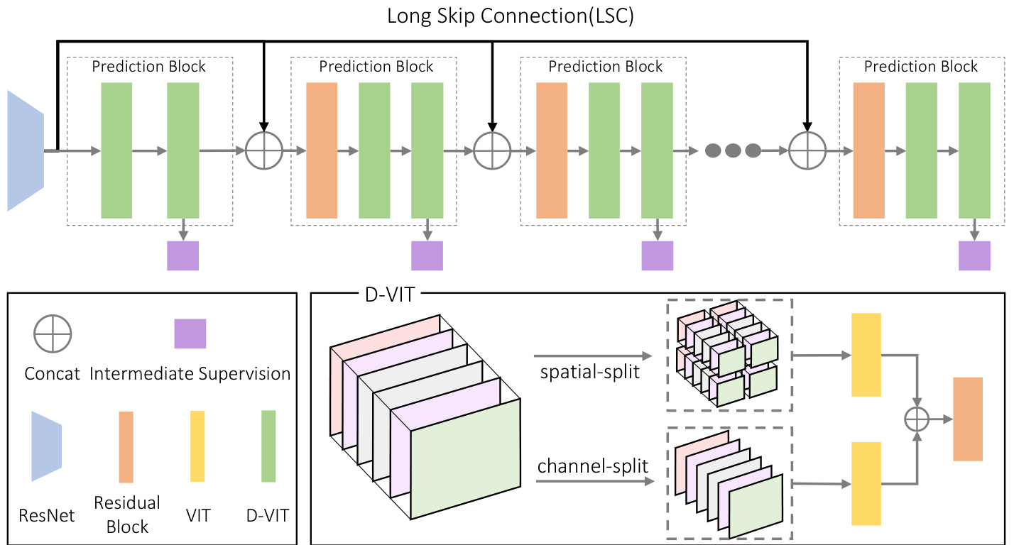
Figure 1. Architecture of our framework. Long skip connections (depicted as upper black lines) distribute low-level features to each prediction block, thereby preventing useful information from being discarded by intermediate supervision. D-ViT learns contextual features of the image through spatially split patches and captures the underlying geometric relations among landmarks using channel-split features.
图 1: 本框架架构示意图。长跳跃连接(图中上方黑线)将底层特征分发至每个预测模块,从而防止有效信息被中间监督丢弃。D-ViT通过空间分块学习图像的上下文特征,并利用通道分割特征捕捉关键点间的几何关联。
3.1. Dual Vision Transformer
3.1. 双视觉Transformer (Dual Vision Transformer)
Our dual vision transformer (D-ViT) is built upon the standard vision transformer (ViT) [10], which disc ret ize s the input image or feature map into smaller spatial patches and arranges these patches into a sequence. Then, the attention mechanism is utilized to establish relationships among the patches, allowing for the extraction of both local and global image features. However, the standard ViT does not explicitly leverage the geometric relationships among landmarks. Consequently, we propose to incorporate a channelsplit ViT to establish the relationships between bases in the heatmap space, thereby extracting the underlying geometric features among landmarks. The proposed channel-split ViT can be seamlessly integrated into the ViT architecture without the need for extra steps, such as explicit conversion to the heatmaps or landmark coordinates. Finally, the spatialsplit ViT and the channel-split ViT together form our Dual Vision Transformer (D-ViT), as shown in Fig. 1.
我们的双视觉Transformer (D-ViT) 基于标准视觉Transformer (ViT) [10]构建,后者将输入图像或特征图离散化为较小的空间块,并将这些块排列成序列。然后利用注意力机制建立块之间的关系,从而提取局部和全局图像特征。然而,标准ViT并未显式利用地标间的几何关系。因此,我们提出引入通道分割ViT来建立热图空间中基向量之间的关系,从而提取地标间的底层几何特征。所提出的通道分割ViT可以无缝集成到ViT架构中,无需额外步骤(例如显式转换为热图或地标坐标)。最终,空间分割ViT与通道分割ViT共同构成了我们的双视觉Transformer (D-ViT),如图1所示。
The design of the channel-split ViT is based on the insight that the channel dimension of feature maps essentially represents the bases of the heatmap space. Specifically, in the architecture, the prediction block outputs a feature map $\boldsymbol{F}\in\mathbb{R}^{C\times H\times W}$ for intermediate supervision, where $C,H$ and $W$ denote the number of channels, height, and width. Then, the feature map $F$ can be split along the channels into $F=(f_{1},f_{2},...,f_{C})$ , where $f_{m}\in\mathbb{R}^{H\times W}$ . Therefore, when considering using convolution operations to regress the feature map $F$ into the heatmaps, the heatmap for each landmark in the intermediate supervision is actually a linear combination of $f_{m}$ :
通道分离ViT的设计基于这样的洞察:特征图的通道维度本质上代表了热图空间的基。具体而言,在该架构中,预测块会输出一个特征图$\boldsymbol{F}\in\mathbb{R}^{C\times H\times W}$用于中间监督,其中$C,H$和$W$分别表示通道数、高度和宽度。然后,特征图$F$可以沿通道维度拆分为$F=(f_{1},f_{2},...,f_{C})$,其中$f_{m}\in\mathbb{R}^{H\times W}$。因此,当考虑使用卷积操作将特征图$F$回归为热图时,中间监督中每个关键点的热图实际上是$f_{m}$的线性组合:
$$
h_{i}=\sum_{m=1}^{C}\alpha_{m}^{i}f_{m},\quad(i=1,2,...,M),
$$
$$
h_{i}=\sum_{m=1}^{C}\alpha_{m}^{i}f_{m},\quad(i=1,2,...,M),
$$
where $M$ is the number of landmarks, $h_{i}$ is the heatmap of $i$ -th landmark, and $\alpha_{m}^{i}$ is learnable parameters. In experiment, such linear combination can be implemented using a Conv2D layer with $1\times1$ kernel. Besides, Fig. 2 presents a visual explanation.
其中 $M$ 是地标(landmark)数量,$h_{i}$ 表示第 $i$ 个地标的热力图(heatmap),$\alpha_{m}^{i}$ 是可学习参数。实验中,该线性组合可通过 $1\times1$ 卷积核(Conv2D)层实现。此外,图 2: 提供了可视化说明。
Eq. (1) and Fig. 2 show that the separated sub feature maps $(f_{1},f_{2},...,f_{C})$ are actually linear bases of the heatmap space. Since the heatmaps determine the coordinates of the landmarks, we can capture the inherent geometric relations among landmarks by analyzing the relations among the linear bases of heatmap space.
式 (1) 和图 2 表明,分离的子特征图 $(f_{1},f_{2},...,f_{C})$ 实际上是热图空间的线性基。由于热图决定了关键点的坐标,我们可以通过分析热图空间线性基之间的关系来捕捉关键点之间固有的几何关系。
In our implementation, we utilize transformer to capture the inherent relationships among the linear bases $(f_{1},f_{2}$ , $...,f_{C})$ , allowing for adaptive computation of their interconnections through the multi-head self-attention mechanism, which is the core component of the transformer architecture [41]. For self-contained ness, we briefly describe the self-attention mechanism. It projects an input sequence $X\in\mathbb{R}^{L\times d}$ into query $Q\in\mathbb{R}^{L\times d}$ , key $K\in\mathbb{R}^{L\times d}$ , and value $V\in\mathbb{R}^{L\times d}$ by three learnable matrices. The attention mechanism is formulated as follows:
在我们的实现中,我们利用Transformer来捕捉线性基$(f_{1},f_{2}$ , $...,f_{C})$之间的内在关系,通过多头自注意力机制自适应地计算它们之间的相互联系,这是Transformer架构的核心组件[41]。为了完整性,我们简要描述一下自注意力机制。它将输入序列$X\in\mathbb{R}^{L\times d}$通过三个可学习矩阵投影为查询$Q\in\mathbb{R}^{L\times d}$、键$K\in\mathbb{R}^{L\times d}$和值$V\in\mathbb{R}^{L\times d}$。注意力机制的计算公式如下:
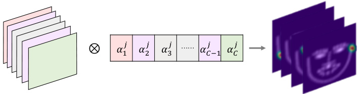
Figure 2. Heatmap is linear combination of channel-split features. $\otimes$ denotes dot-product. Intermediate supervision uses Conv2D with $1\times1$ kernel to convert the features extracted from a prediction block into heatmaps. This implies channel-split features linearly expand the heatmap space. Based on this observation, we take advantage of the self-attention mechanism to learn underlying geometric relations among landmarks via channel-split features.
图 2: 热力图是通道分割特征的线性组合。$\otimes$表示点积运算。中间监督采用 $1\times1$ 卷积核的 Conv2D 层,将预测块提取的特征转换为热力图。这表明通道分割特征能够线性扩展热力图空间。基于这一观察,我们利用自注意力机制 (self-attention) 通过通道分割特征学习地标点之间的潜在几何关系。
$$
A t t e n t i o n(Q,K,V)=s o f t m a x(\frac{Q K^{T}}{\sqrt{d}})V.
$$
$$
A t t e n t i o n(Q,K,V)=s o f t m a x(\frac{Q K^{T}}{\sqrt{d}})V.
$$
Then, our D-ViT is formally defined as:
随后,我们的D-ViT正式定义为:
$$
D-V i T=C o n v\big(V i T(P a t)||V i T(C h n)\big),
$$
$$
D-V i T=C o n v\big(V i T(P a t)||V i T(C h n)\big),
$$
where $P a t$ denotes the spatial-split patches, Chn represents the channel-split features, $||$ refers to concatenation along the channel dimension and $C o n v(\cdot)$ is a residual convolution block. Beneficial from such design, our D-ViT can leverage both spatial-split patches and channel-split features to extract image features and establish inherent relations among landmarks, thereby achieving new state-of-the-art results across three benchmarks. In the following discussion, we refer to the standard ViT with spatially split patches as spatial-split ViT, and the ViT with channel-split features as channel-split ViT.
其中 $P a t$ 表示空间分割块 (spatial-split patches),Chn 代表通道分割特征 (channel-split features),$||$ 指沿通道维度的拼接操作,$C o n v(\cdot)$ 为残差卷积块。得益于这种设计,我们的 D-ViT 能够同时利用空间分割块和通道分割特征来提取图像特征并建立关键点间的内在关联,从而在三个基准测试中均取得了最先进的成果。在下文讨论中,我们将标准空间分割的 ViT 称为空间分割 ViT (spatial-split ViT),将通道分割的 ViT 称为通道分割 ViT (channel-split ViT)。
3.2. Long Skip Connection
3.2. 长跳跃连接
Following the design paradigm of the widely used hourglasses networks [29, 52], which often serve as backbones for facial landmark detection [18, 21, 29, 44, 54], we repeat the prediction block in conjunction with intermediate supervision to consolidate feature processing. However, we found that when using residual connections between two sequential prediction blocks (i.e., ResCBSP in Fig. 5a), the detection performance is instead diminished by deeper prediction blocks. More details can be found in the ablation study in Sec. 4.3.
遵循广泛使用的沙漏网络 [29, 52] 的设计范式(该架构常作为面部关键点检测 [18, 21, 29, 44, 54] 的主干网络),我们通过重复预测块并结合中间监督来强化特征处理。但实验发现,当在两个连续预测块之间使用残差连接(即图 5a 中的 ResCBSP)时,更深的预测块反而会降低检测性能。更多细节见第 4.3 节的消融实验。
The reason of this behavior is the supervision of outputs from intermediate prediction blocks. Specifically, during training, supervision at all intermediate stages compels the network to extract relevant information for estimating landmarks. However, this can also lead to the loss of some information; since shallow prediction blocks may not perform optimally, they might inadvertently discard useful information that could be better processed by deeper prediction blocks.
这种行为的原因在于对中间预测块输出的监督。具体来说,在训练过程中,所有中间阶段的监督迫使网络提取用于估计地标的相关信息。然而,这也可能导致一些信息的丢失;由于浅层预测块可能无法达到最佳性能,它们可能会无意中丢弃一些本可以由更深层预测块更好处理的有用信息。
Therefore, unlike previous methods that use residual connections between two consecutive prediction blocks, we propose using long skip connections (LSC) to distribute low-level image features, thereby making deeper network architectures feasible. Specifically, the LSC (shown as the upper black line in Fig. 1) originates from the low-level image features extracted by ResNet and transmits these features to each prediction block. As a result, each intermediate prediction block receives features extracted from the previous block as well as the complete low-level features.
因此,不同于以往方法在两个连续预测块之间使用残差连接,我们提出采用长跳跃连接 (LSC) 来传递底层图像特征,从而使更深层的网络架构成为可能。具体而言,LSC (如图 1 上方黑线所示) 源自 ResNet 提取的底层图像特征,并将这些特征传递至每个预测块。这使得每个中间预测块既能接收前一个块提取的特征,又能获得完整的底层特征。
3.3. Training Loss
3.3. 训练损失
We adopt the widely used soft-argmax operator to decode heatmaps into landmark positions. Let $\mathbf{\dot{\Phi}}{h_{i}^{j}}$ denote the heatmap for the $i$ -th landmark predicted by $j$ -th intermediate supervision. We denote the $k$ -th pixel position in the heatmap as $g_{k}$ and the heatmap value at $g_{k}$ as $h_{i k}^{j}$ . The cor- responding landmark location for heatmap $h_{i}^{j}$ is given by:
我们采用广泛使用的软性argmax算子将热图解码为关键点位置。设 $\mathbf{\dot{\Phi}}{h_{i}^{j}}$ 表示第 $j$ 个中间监督预测的第 $i$ 个关键点的热图。将热图中第 $k$ 个像素位置记为 $g_{k}$ ,该位置的热图值为 $h_{i k}^{j}$ 。热图 $h_{i}^{j}$ 对应的关键点位置由下式给出:
$$
\mu_{i}^{j}=\sum_{k=1}^{H\times W}h_{i k}^{j}g_{k}.
$$
$$
\mu_{i}^{j}=\sum_{k=1}^{H\times W}h_{i k}^{j}g_{k}.
$$
The loss for the $j$ -th intermediate supervision consists of two components: one for supervising landmark coordinates and the other for supervising the heatmaps, as shown in the following formula:
第 $j$ 个中间监督的损失由两部分组成:一部分用于监督地标坐标,另一部分用于监督热图,如下式所示:
$$
\mathcal{L}{j}=\sum_{i}\big(d_{1}(\mu_{i}^{j},y_{i})+\beta d_{2}(h_{i}^{j},z_{i})\big),
$$
$$
\mathcal{L}{j}=\sum_{i}\big(d_{1}(\mu_{i}^{j},y_{i})+\beta d_{2}(h_{i}^{j},z_{i})\big),
$$
where $y_{i}$ is the ground truth location of the $i$ -th landmark, and $z_{i}$ is the corresponding heatmap defined by a Gaussian kernel. $\beta$ is a balance weight between coordinate and heatmap regression. $d_{1}$ and $d_{2}$ are loss functions for regressing coordinates and heatmaps. In this paper, we utilize smooth-L1 as $d_{1}$ and awing loss [44] as $d_{2}$ .
其中 $y_{i}$ 是第 $i$ 个关键点的真实位置,$z_{i}$ 是由高斯核定义的对应热图。$\beta$ 是坐标回归与热图回归之间的平衡权重。$d_{1}$ 和 $d_{2}$ 分别用于回归坐标和热图的损失函数。本文采用 smooth-L1 作为 $d_{1}$,并选用 awing loss [44] 作为 $d_{2}$。
The total loss for optimizing our network is a combination of the loss terms from each intermediate supervision:
优化我们网络的总损失是各中间监督损失项的组合:
$$
\mathcal{L}{t o t a l}=\sum_{j=1}^{B}w^{j-B}\mathcal{L}_{j},
$$
$$
\mathcal{L}{t o t a l}=\sum_{j=1}^{B}w^{j-B}\mathcal{L}_{j},
$$
where $B$ is the number of prediction blocks, and $w(w\ge1)$ is an expanding factor that balances intermediate supervisions across different block outputs.
其中 $B$ 是预测块的数量,$w(w\ge1)$ 是平衡不同块输出间中间监督的扩展因子。
4. Experiments
4. 实验
In this section, we first introduce the experimental setup, including the datasets, evaluation metrics, and the implementation details in Section 4.1. Then, we compare our approach with state-of-the-art face landmark detection methods in Section 4.2. Finally, we perform ablation studies to analyze the design of our framework in Section 4.3.
在本节中,我们首先在第4.1节介绍实验设置,包括数据集、评估指标和实现细节。然后在第4.2节将我们的方法与最先进的人脸关键点检测方法进行比较。最后在第4.3节进行消融实验以分析我们框架的设计。
4.1. Experimental Setup
4.1. 实验设置
Datasets. For experimental evaluation, we consider three widely used datasets: WFLW [45], COFW [3], and 300W [34]. Additionally, in the ablation experiments, we also employed a video-based dataset WFLW-V [28] for cross-dataset validation. The WFLW dataset is based on the WIDER dataset [48] and includes 7,500 training images and 2,500 test images, each with 98 labeled keypoints. The test set is further divided into six subsets: large-pose, expression, illumination, makeup, occlusion and blur, to assess algorithm performance under various conditions. For this dataset, we use the pre-cropped WFLW dataset from Lan et al. [21] in our experiments. The COFW dataset features heavy occlusions and a wide range of head poses, comprising 1,345 training images and 507 test images. Each face is annotated with 29 landmarks. 300W dataset is a widely adopted dataset for face alignment and contains 3,148 images for training and 689 images for testing. The test set is divided into two subsets: common and challenge. All images are labeled with 68 landmarks. The WFLW-V dataset provides 1,000 videos, which are equally categorized into easy and hard subsets. In the cross-dataset validation, we train our model on the WFLW dataset and test it on every video frame from WFLW-V dataset.
数据集。为进行实验评估,我们采用了三个广泛使用的数据集:WFLW [45]、COFW [3] 和 300W [34]。此外,在消融实验中,我们还使用了基于视频的数据集 WFLW-V [28] 进行跨数据集验证。WFLW 数据集基于 WIDER 数据集 [48],包含 7,500 张训练图像和 2,500 张测试图像,每张图像标注了 98 个关键点。测试集进一步划分为六个子集:大姿态、表情、光照、化妆、遮挡和模糊,用于评估算法在不同条件下的性能。对于该数据集,我们在实验中使用了 Lan 等人 [21] 提供的预裁剪 WFLW 数据集。COFW 数据集以严重遮挡和多样头部姿态为特点,包含 1,345 张训练图像和 507 张测试图像,每张人脸标注了 29 个特征点。300W 数据集是人脸对齐领域广泛采用的数据集,包含 3,148 张训练图像和 689 张测试图像,测试集划分为常见和挑战两个子集,所有图像均标注了 68 个特征点。WFLW-V 数据集提供了 1,000 段视频,平均分为简单和困难两个子集。在跨数据集验证中,我们在 WFLW 数据集上训练模型,并在 WFLW-V 数据集的每帧视频图像上进行测试。
Evaluation Metrics. For quantitative evaluation, three commonly used metrics are adopted: Normalized Mean Error (NME), Failure Rate (FR), and Area Under Curve (AUC). To calculate NME, we use the inter ocular distance for normalization in the WFLW and 300W datasets, and the inter pupils distance for normalization in the COFW dataset. Same with previous works like STAR [54] and LDEQ [28], we report FR and AUC for the WFLW dataset with the cutoff threshold $10%$ . For NME and FR, lower values indicate better performance, while for AUC, a higher value is preferable.
评估指标。定量评估采用三种常用指标:归一化平均误差 (NME)、失败率 (FR) 和曲线下面积 (AUC)。计算 NME 时,WFLW 和 300W 数据集使用眼间距归一化,COFW 数据集使用瞳孔间距归一化。与 STAR [54] 和 LDEQ [28] 等先前工作相同,我们对 WFLW 数据集报告 FR 和 AUC 时采用 $10%$ 的截止阈值。NME 和 FR 值越低表示性能越好,而 AUC 值越高越好。
Implementation Details. For the images fed into our network, the face regions are cropped and resized to $256\times$ 256. Common image augmentations have been applied including random rotation, random translation, random occlusion, random blur, random color jitter, random horizontal flip, and random grayscale conversion. In our network, ResNet [15] is utilized to extract low-level image features. The ResNet in our model is built with bottleneck structure, and its number of parameters is about $13%$ of the standard ResNet50. We stack 8 prediction blocks to sequentially predict $256\times32\times32$ feature maps for intermediate supervision. In spatial-split ViT, we apply a Conv2d layer for patch embedding. In channel-split ViT, we use another Conv2d layer to halve the spatial size to save memory. At the end of channel-split or spatial-split ViT, pixel shuffle [35] is used to restore the spatial dimensions to $32\times32$ . More implementation details about D-ViT are shown in Fig. 3. Groundtruth heatmaps are generated by the 2-dimensional Gaussian distribution with small variance [50]. We employ the Adam optimizer with initial learning rate $1\times10^{-4}$ . The learning rate is reduced by half for every 200 epochs, and we optimize the network parameters for a totoal of 500 epochs. The model is trained on two GPUs (Nvidia V100 16G), with a batch size of 16 per GPU.
实现细节。输入网络的图像会进行面部区域裁剪并调整至$256\times$256大小。应用了包括随机旋转、随机平移、随机遮挡、随机模糊、随机色彩抖动、随机水平翻转和随机灰度转换在内的常规图像增强方法。网络采用ResNet[15]提取低级图像特征,该ResNet采用瓶颈结构构建,参数量约为标准ResNet50的$13%$。我们堆叠8个预测块来顺序预测$256\times32\times32$特征图以进行中间监督。在空间分割ViT中,使用Conv2d层进行块嵌入;在通道分割ViT中,采用另一个Conv2d层将空间尺寸减半以节省内存。通道分割或空间分割ViT末端通过像素重组[35]将空间维度恢复至$32\times32$。D-ViT更多实现细节如图3所示。真值热图通过小方差二维高斯分布生成[50]。采用初始学习率为$1\times10^{-4}$的Adam优化器,每200轮次学习率减半,共优化500轮次。模型在两张GPU(Nvidia V100 16G)上训练,每GPU批大小为16。
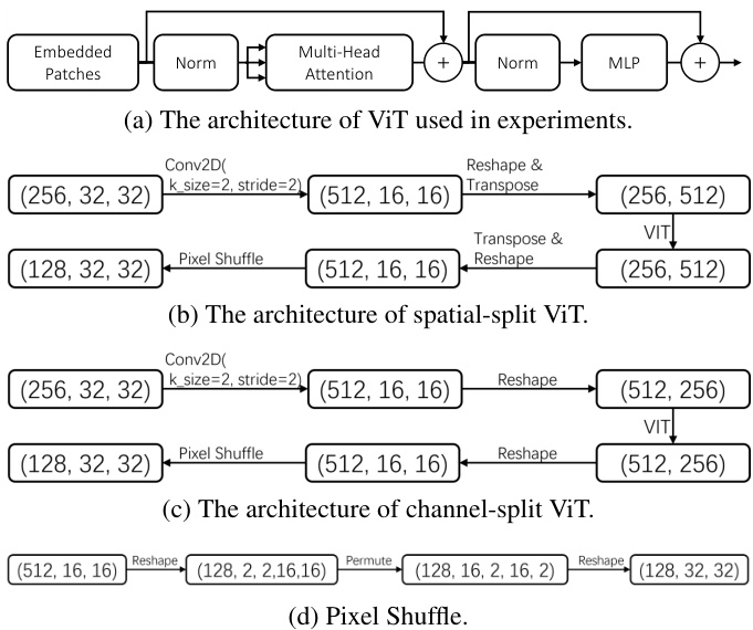
Figure 3. Implementation details of our D-ViT.
图 3: 我们的 D-ViT 实现细节。
4.2. Comparison on Detection Accuracy
4.2. 检测精度对比
In this section, we compare our method with previous state-of-the-art baselines. The NME across three datasets are reported in Tab. 1, while the FR and AUC for WFLW dataset are shown in Tab. 2. The results presented in both tables demonstrate that our approach surpasses the previous baselines and achieves a new SOTA across all three datasets.
在本节中,我们将我们的方法与之前的最先进基线进行比较。三个数据集的NME如表1所示,而WFLW数据集的FR和AUC如表2所示。两个表格中呈现的结果表明,我们的方法超越了之前的基线,并在所有三个数据集上实现了新的SOTA。
Compared to other transformer-based methods [23, 46], our approach achieves an improvement of 0.33 and 0.37 in NME on the full WFLW dataset over DTLD [23] and SLPT [46], respectively. This demonstrates that our proposed D-ViT and long skip connection have a positive impact on the performance of transformers. Additionally, our proposal also outperforms recent CNN-based methods [28, 54] that achieved state-of-the-art results. Specifically, our NME score is 0.27 and 0.17 better than that of STAR [54] and LDEQ [28] on the full WFLW test set. Fur- thermore, for the Pose and Occlusion subsets, which contain severe occlusions, our method significantly improves the detection performance, demonstrating that our network is capable of capturing the contextual features of images and the intrinsic relationships between landmarks.
与其他基于Transformer的方法[23,46]相比,我们的方法在完整WFLW数据集上的NME指标分别比DTLD[23]和SLPT[46]提高了0.33和0.37。这表明我们提出的D-ViT和长跳跃连接对Transformer性能有积极影响。此外,我们的方案也优于近期取得最先进结果的基于CNN的方法[28,54],在完整WFLW测试集上,我们的NME分数比STAR[54]和LDEQ[28]分别高出0.27和0.17。特别是在包含严重遮挡的Pose和Occlusion子集上,我们的方法显著提升了检测性能,证明网络能够有效捕捉图像上下文特征和关键点之间的内在关联。
Table 1. Quantitative comparison with previous state-of-the-art methods on three public datasets using the NME metric. The best and second best results are marked in colors of red and blue, respectively. It can be seen that our method achieves new SOTA results on the full test sets of all three datasets.
| Method | WFLW | COFW | 300W | |||||||||
| Full | Pose | Expr. | Illum. | Makeup | Occl. | Blur | Full | Full | Comm. | Chal. | ||
| LAB [45] | CVPR'18 | 5.27 | 10.24 | 5.51 | 5.23 | 5.15 | 6.79 | 6.32 | 3.49 | 2.98 | 5.19 | |
| Wing [12] | CVPR'18 | 4.99 | 8.43 | 5.21 | 4.88 | 5.26 | 6.21 | 5.81 | 5.44 | |||
| DecaFA [6] | ICCV'19 | 4.62 | 8.11 | 4.65 | 4.41 | 4.63 | 5.74 | 5.38 | 3.39 | 2.93 | 5.26 | |
| HRNet [37] | CVPR'19 | 4.60 | 7.94 | 4.85 | 4.55 | 4.29 | 5.44 | 5.42 | 3.32 | 2.87 | 5.15 | |
| AS [32] | ICCV'19 | 4.39 | 8.42 | 4.68 | 4.24 | 4.37 | 5.60 | 4.86 | 3.86 | 3.21 | 6.46 | |
| LUVLI [20] | CVPR'20 | 4.37 | 7.56 | 4.77 | 4.30 | 4.33 | 5.29 | 4.94 | 3.23 | 2.76 | 5.16 | |
| AWing [44] | ICCV'19 | 4.36 | 7.38 | 4.58 | 4.32 | 4.27 | 5.19 | 4.96 | 4.94 | 3.07 | 2.72 | 4.52 |
| SDL [24] | ECCV'20 | 4.21 | 7.36 | 4.49 | 4.12 | 4.05 | 4.98 | 4.82 | 3.04 | 2.62 | 4.77 | |
| ADNet [18] | ICCV'21 | 4.14 | 6.96 | 4.38 | 4.09 | 4.05 | 5.06 | 4.79 | 4.68 | 2.93 | 2.53 | 4.58 |
| SLPT [46] | CVPR'22 | 4.12 | 6.99 | 4.37 | 4.02 | 4.03 | 5.01 | 4.79 | 4.79 | 3.17 | 2.75 | 4.90 |
| HIH [21] | ICCVW'21 | 4.08 | 6.87 | 4.06 | 4.34 | 3.85 | 4.85 | 4.66 | 4.63 | 3.09 | 2.65 | 4.89 |
| DTLD [23] | CVPR'22 | 4.08 | 一 | 2.96 | 2.59 | 4.50 | ||||||
| SPIGA [31] | BMVC'22 | 4.06 | 7.14 | 4.46 | 4.00 | 3.81 | 4.95 | 4.65 | ||||
| STAR [54] | CVPR'23 | 4.02 | 6.79 | 4.27 | 3.97 | 3.84 | 4.80 | 4.58 | 4.62 | 2.87 | 2.52 | 4.32 |
| LDEQ [28] | CVPR'23 | 3.92 | 6.86 | 3.94 | 4.17 | 3.75 | 4.77 | 4.59 | ||||
| FRA [13] | CVPR'24 | 4.11 | 2.91 | 2.60 | 4.46 | |||||||
| Ours | 3.75 | 6.43 | 3.85 | 4.06 | 3.57 | 4.47 | 4.37 | 4.13 | 2.85 | 2.43 | 4.56 | |
表 1: 在三个公开数据集上使用NME指标与先前最优方法的定量比较。最优和次优结果分别用红色和蓝色标出。可以看出,我们的方法在所有三个数据集的完整测试集上都取得了新的SOTA结果。
| 方法 | WFLW | COFW | 300W | ||||||||
|---|---|---|---|---|---|---|---|---|---|---|---|
| Full | Pose | Expr. | Illum. | Makeup | Occl. | Blur | Full | Full | Comm. | ||
| LAB [45] | CVPR'18 | 5.27 | 10.24 | 5.51 | 5.23 | 5.15 | 6.79 | 6.32 | 3.49 | 2.98 | |
| Wing [12] | CVPR'18 | 4.99 | 8.43 | 5.21 | 4.88 | 5.26 | 6.21 | 5.81 | 5.44 | ||
| DecaFA [6] | ICCV'19 | 4.62 | 8.11 | 4.65 | 4.41 | 4.63 | 5.74 | 5.38 | 3.39 | 2.93 | |
| HRNet [37] | CVPR'19 | 4.60 | 7.94 | 4.85 | 4.55 | 4.29 | 5.44 | 5.42 | 3.32 | 2.87 | |
| AS [32] | ICCV'19 | 4.39 | 8.42 | 4.68 | 4.24 | 4.37 | 5.60 | 4.86 | 3.86 | 3.21 | |
| LUVLI [20] | CVPR'20 | 4.37 | 7.56 | 4.77 | 4.30 | 4.33 | 5.29 | 4.94 | 3.23 | 2.76 | |
| AWing [44] | ICCV'19 | 4.36 | 7.38 | 4.58 | 4.32 | 4.27 | 5.19 | 4.96 | 4.94 | 3.07 | 2.72 |
| SDL [24] | ECCV'20 | 4.21 | 7.36 | 4.49 | 4.12 | 4.05 | 4.98 | 4.82 | 3.04 | 2.62 | |
| ADNet [18] | ICCV'21 | 4.14 | 6.96 | 4.38 | 4.09 | 4.05 | 5.06 | 4.79 | 4.68 | 2.93 | 2.53 |
| SLPT [46] | CVPR'22 | 4.12 | 6.99 | 4.37 | 4.02 | 4.03 | 5.01 | 4.79 | 4.79 | 3.17 | 2.75 |
| HIH [21] | ICCVW'21 | 4.08 | 6.87 | 4.06 | 4.34 | 3.85 | 4.85 | 4.66 | 4.63 | 3.09 | 2.65 |
| DTLD [23] | CVPR'22 | 4.08 | 一 | 2.96 | 2.59 | ||||||
| SPIGA [31] | BMVC'22 | 4.06 | 7.14 | 4.46 | 4.00 | 3.81 | 4.95 | 4.65 | |||
| STAR [54] | CVPR'23 | 4.02 | 6.79 | 4.27 | 3.97 | 3.84 | 4.80 | 4.58 | 4.62 | 2.87 | 2.52 |
| LDEQ [28] | CVPR'23 | 3.92 | 6.86 | 3.94 | 4.17 | 3.75 | 4.77 | 4.59 | |||
| FRA [13] | CVPR'24 | 4.11 | 2.91 | 2.60 | |||||||
| Ours | 3.75 | 6.43 | 3.85 | 4.06 | 3.57 | 4.47 | 4.37 | 4.13 | 2.85 | 2.43 |
Table 2. $\mathrm{FR}{10}$ and $\mathrm{{AUC}_{10}}$ on the WFLW test set. The best and second best results are marked in colors of red and blue, respectively. The results demonstrate the robustness and effectiveness of our proposed model.
表 2. WFLW测试集上的$\mathrm{FR}{10}$和$\mathrm{AUC}_{10}$。最佳和次佳结果分别用红色和蓝色标出。结果表明了我们提出模型的鲁棒性和有效性。
| 方法 | FR10(↓) | AUC10(↑) | ||||||||||||
|---|---|---|---|---|---|---|---|---|---|---|---|---|---|---|
| Full | Pose | Exp. | Ill. | Mu. | Occ. | Blur | Full | Pose | Exp. | Ill. | Mu. | Occ. | Blur | |
| LAB [45] | 7.56 | 28.83 | 6.37 | 6.73 | 7.77 | 13.72 | 10.74 | 53.2 | 23.5 | 49.5 | 54.3 | 53.9 | 44.9 | 46.3 |
| HRNet [37] | 4.64 | 23.01 | 3.5 | 4.72 | 2.43 | 8.29 | 6.34 | 52.4 | 25.1 | 51 | 53.3 | 54.5 | 45.9 | 45.2 |
| AS [32] | 4.08 | 18.1 | 4.46 | 2.72 | 4.37 | 7.74 | 4.4 | 59.1 | 31.1 | 54.9 | 60.9 | 58.1 | 51.6 | 55.1 |
| LUVLi [20] | 3.12 | 15.95 | 3.18 | 2.15 | 3.4 | 6.39 | 3.23 | 55.7 | 31 | 54.9 | 58.4 | 58.8 | 50.5 | 52.5 |
| AWing [44] | 2.84 | 13.5 | 2.23 | 2.58 | 2.91 | 5.98 | 3.75 | 57.2 | 31.2 | 51.5 | 57.8 | 57.2 | 50.2 | 51.2 |
| SDL [24] | 3.04 | 15.95 | 2.86 | 2.72 | 1.45 | 5.29 | 4.01 | 58.9 | 31.5 | 56.6 | 59.5 | 60.4 | 52.4 | 53.3 |
| ADNet [18] | 2.72 | 12.72 | 2.15 | 2.44 | 1.94 | 5.79 | 3.54 | 60.2 | 34.4 | 52.3 | 58 | 60.1 | 53 | 54.8 |
| SLPT [46] | 2.72 | 11.96 | 1.59 | 2.15 | 1.94 | 5.7 | 3.88 | 59.6 | 34.9 | 57.3 | 60.3 | 60.8 | 52 | 53.7 |
| HIH [21] | 2.6 | 12.88 | 1.27 | 2.43 | 1.45 | 5.16 | 3.1 | 60.5 | 35.8 | 60.1 | 61.3 | 61.8 | 53.9 | 56.1 |
| FRA [13] | 2.53 | - | 59.1 | |||||||||||
| SPIGA [31] | 2.08 | 11.66 | 2.23 | 1.58 | 1.46 | 4.48 | 2.2 | 60.6 | 35.3 | 58 | 61.3 | 62.2 | 53.3 | 55.3 |
| STAR [54] | 2.32 | 11.69 | 2.24 | 1.58 | 0.98 | 4.76 | 3.24 | 60.5 | 36.2 | 58.4 | 60.9 | 62.2 | 53.8 | 55.1 |
| LDEQ [28] | 2.48 | 12.58 | 1.59 | 2.29 | 1.94 | 5.36 | 2.84 | 62.4 | 37.3 | 61.4 | 63.1 | 63.1 | 55.2 | 57.4 |
| Ours | 1.76 | 8.28 | 1.27 | 1.29 | 1.94 | 3.8 | 2.07 | 63.7 | 40.1 | 62.6 | 64.7 | 64.7 | 57.1 | 58.6 |
By exploring the relationships between bases in the heatmap space to model the underlying geometric relations among landmarks, our method achieves a significant improvement of 0.49 in NME on the COFW dataset, which contains heavy occlusions and a wide range of head poses, compared to the previous SOTA baseline, STAR [54].
通过探索热图空间中基准点之间的关系来建模地标之间的潜在几何关联,我们的方法在包含严重遮挡和多种头部姿态的COFW数据集上,相比之前的SOTA基线STAR [54],NME指标显著提升了0.49。

Figure 4. Qualitative results of different prediction blocks on WFLW dataset. Green and red points represent the predicted and ground-truth landmarks, respectively. Orange or Yellow circles indicate the clear failures, which can be improved with help of D-ViT. Table 3. Comparisons of different connection strategies and different prediction blocks on dataset COFW and 300W by using 8 prediction blocks. NME scores are reported.
图 4: WFLW数据集上不同预测模块的定性结果。绿色和红色点分别代表预测关键点和真实关键点。橙色或黄色圆圈标明了明显错误区域,这些区域可通过D-ViT得到改善。
表 3: 在COFW和300W数据集上使用8个预测模块时,不同连接策略与不同预测模块的对比结果(报告NME分数)。
| Dataset | Connection Strategy | Block Name | ||||
| ResCBSP | DenC | LSC | Spatial-split | Channel-split | D-ViT | |
| COFW | 4.14 | 4.14 | 4.13 | 4.18 | 4.20 | 4.13 |
| 300W | 2.89 | 2.90 | 2.85 | 2.87 | 2.96 | 2.85 |
| 数据集 | 连接策略 | 模块名称 | ||||
|---|---|---|---|---|---|---|
| ResCBSP | DenC | LSC | Spatial-split | Channel-split | D-ViT | |
| COFW | 4.14 | 4.14 | 4.13 | 4.18 | 4.20 | 4.13 |
| 300W | 2.89 | 2.90 | 2.85 | 2.87 | 2.96 | 2.85 |
Moreover, our approach also achieves the lowest NME on the full $300\mathbf{W}$ test set.
此外,我们的方法在完整的 $300\mathbf{W}$ 测试集上也实现了最低的NME。
The $\mathrm{FR}{10}$ and $\mathrm{AUC_{10}}$ scores on the WFLW dataset, as reported in Tab. 2, demonstrate the robustness and effectiveness of our proposed model. Specifically, our method outperforms previous state-of-the-art methods [28, 31] by 0.32 and 1.30 in $\mathrm{FR}{10}$ and $\mathrm{AUC_{10}}$ , respectively.
在WFLW数据集上的$\mathrm{FR}{10}$和$\mathrm{AUC_{10}}$分数(如表2所示)证明了我们提出模型的稳健性和有效性。具体而言,我们的方法在$\mathrm{FR}{10}$和$\mathrm{AUC_{10}}$上分别以0.32和1.30的优势超越了先前的最先进方法[28, 31]。
4.3. Ablation Studies
4.3. 消融实验
In this section, various ablation studies are conducted to verify the specific design decisions in our model architecture. Discussion about the selections of hyper parameters is also included.
在本节中,我们进行了多项消融实验以验证模型架构中的具体设计决策,同时包含了对超参数选择的讨论。
D-ViT. Our Dual Vision Transformer (D-ViT) utilizes two types of Vision Transformers (ViTs), specifically the spatial-split ViT and channel-split ViT, to extract spatial features from images and underlying geometric features among landmarks, respectively. To demonstrate the necessity of incorporating the channel-split ViT for exploring the relationships between heatmap bases, we report in Tab. 4a the performance on the WFLW dataset when using spatial-split ViT, channel-split ViT, and our proposed D-ViT separately to construct the prediction blocks. Additionally, Tab. 3 presents the NME performance of different prediction blocks on the COFW and 300W datasets. From the two tables, it can be observed that by incorporating the less effective channel-split ViT to construct D-ViT actually leads to more accurate detection. This indicates that exploring relationships among heatmap bases has a positive effect on enhancing accurate predictions. Fig. 4 shows some qualitative visualization s. With the help of D-ViT, our model is able to accurately detect landmarks in various scenarios, such as occlusion, expression, blur, and large pose.
D-ViT。我们的双视觉Transformer (Dual Vision Transformer, D-ViT) 采用两种类型的视觉Transformer (ViT),分别是空间分割ViT和通道分割ViT,分别用于从图像中提取空间特征以及关键点之间的底层几何特征。为了证明引入通道分割ViT对探索热图基之间关系的必要性,表4a展示了单独使用空间分割ViT、通道分割ViT以及我们提出的D-ViT构建预测模块时在WFLW数据集上的性能表现。此外,表3展示了不同预测模块在COFW和300W数据集上的NME性能。从这两个表中可以看出,通过结合效果较弱的通道分割ViT构建D-ViT实际上能带来更精确的检测结果,这表明探索热图基之间的关系对提升预测准确性具有积极作用。图4展示了一些定性可视化结果。借助D-ViT,我们的模型能够在遮挡、表情、模糊和大姿态等多种场景下准确检测关键点。
Table 4. Comparison results of different prediction blocks (a) and different connection strategies (b) with 8 prediction blocks on WFLW dataset.
(b) Quantitative comparison of different connection strategies.
表 4. 不同预测块 (a) 和不同连接策略 (b) 在 WFLW 数据集上的对比结果 (使用 8 个预测块)
| Block Name | NME(↓) | FR10(↓) | AUC10(↑) |
|---|---|---|---|
| Spatial-Split | 3.82 | 2.08 | 63.2 |
| Channel-Split | 3.87 | 2.36 | 63.2 |
| D-ViT | 3.75 | 1.76 | 63.7 |
| (a) 不同预测块的定量对比 | |||
| Conn.Strategy | NME(↓) | FR10(↓) | AUC10(↑) |
| ResCBSP | 3.82 | 2.16 | 63.2 |
| DenC | 3.81 | 2.16 | 63.2 |
| LSC | 3.75 | 1.76 | 63.7 |
(b) 不同连接策略的定量对比。
Long Skip Connection. Connection strategies for prediction blocks are typically either residual connections between sequential predictions (ResCBSP) [16] or dense connections (DenC) [17], as illustrated in Fig. 5a and Fig. 5b. Besides, residual connections are commonly used in stacked Hourglasses (HGs) networks [29,52], which often serve as backbones for facial landmark detection [18, 21, 29, 44, 54]. However, Fig. 6 indicates that using these two strategies to connect prediction blocks built on ViTs results in diminished performance as the number of blocks increases. This is because intermediate supervision can lead to the loss of useful information. To address this, we propose using long skip connections (LSC) to distribute lowlevel image features from ResNet to each prediction block, thereby making deeper network architectures feasible. Additionally, the quantitative comparison of different connection strategies with 8 prediction blocks reported in Tab. 4b on the WFLW dataset, along with the results in Tab. 3 on the COFW and 300W datasets, both demonstrate the superior effectiveness of our proposed LSC.
长跳跃连接 (Long Skip Connection)。预测块之间的连接策略通常有两种:顺序预测间的残差连接 (ResCBSP) [16] 或密集连接 (DenC) [17],如图 5a 和图 5b 所示。此外,残差连接也常用于堆叠沙漏网络 (HGs) [29,52],这类网络常作为面部关键点检测的骨干网络 [18, 21, 29, 44, 54]。然而,图 6 表明,当使用这两种策略连接基于 ViT 构建的预测块时,随着块数增加会导致性能下降。这是因为中间监督可能导致有用信息丢失。为解决这一问题,我们提出使用长跳跃连接 (LSC) 将 ResNet 的低层图像特征分发至每个预测块,从而使更深层的网络架构成为可能。此外,表 4b 中 WFLW 数据集上 8 个预测块的不同连接策略定量比较,以及表 3 中 COFW 和 300W 数据集上的结果,均证明了我们提出的 LSC 具有更优效果。

Figure 5. Illustrations of alternative skip connections. ResCBSP denotes the residual connections between two sequential prediction blocks. DenC denotes dense connections where any two prediction blocks have a skip connection. Refer to Fig. 1 for definition of prediction block and colorful rectangles.
图 5: 替代跳跃连接的示意图。ResCBSP 表示两个连续预测块之间的残差连接。DenC 表示密集连接,其中任意两个预测块之间都有跳跃连接。预测块和彩色矩形的定义请参考图 1。

Figure 6. NME against number of prediction blocks on WFLW dataset. When the number is 2, three strategies essentially represent the same structure. When the number exceeds 4, the performance of $\mathrm{ResCBSP}$ or DenC starts to get worse. While with our proposed LSC, the model can benefit from a deeper architecture.
图 6: WFLW数据集上NME随预测块数量的变化。当数量为2时,三种策略本质上代表相同结构。当数量超过4时,$\mathrm{ResCBSP}$或DenC的性能开始下降。而采用我们提出的LSC时,模型能从更深层架构中获益。
Cross-dataset Validations. To further validate our design decisions, we conduct a cross-dataset validation experiment that includes quantitative comparisons of different prediction blocks and connection strategies, similar to the one described in Tab. 4. However, different from that experiment, we train the models on the WFLW dataset and evaluate them on subsets of the WFLW-V dataset, i.e., the easy set and the hard set. The results reported in Tab. 5 indicate that our proposed D-ViT and LSP still achieve the best NME score in the cross-dataset validations, demonstrating superior generalization.
跨数据集验证。为进一步验证我们的设计决策,我们进行了跨数据集验证实验,包括对不同预测模块和连接策略的定量比较,类似于表4所述实验。不同的是,本次实验在WFLW数据集上训练模型,并在WFLW-V数据集的子集(即简单集和困难集)上进行评估。表5结果显示,我们提出的D-ViT和LSP在跨数据集验证中仍能取得最佳NME分数,展现出卓越的泛化能力。
Weight for Intermediate Supervision. Weight $w$ in Eq. (6) is a balance between multiple intermediate supervisions. To study the influence, we carried out experiments with $w$ ranging from 1.0 to 1.6, as shown in Tab. 6. Our model achieves the best performance with $w$ set to 1.2. Thus, we choose 1.2 as the default setting.
中间监督权重。式 (6) 中的权重 $w$ 用于平衡多个中间监督信号。为研究其影响,我们在 $w$ 取值为 1.0 至 1.6 的范围内进行了实验,如 表 6 所示。当 $w$ 设为 1.2 时,我们的模型取得了最佳性能,因此选择 1.2 作为默认设置。
(a) Quantitative comparison of different prediction blocks.
| Block Name | Easy | Hard |
|---|---|---|
| Spatial-split | 1.74 | 2.96 |
| Channel-split | 1.69 | 3.12 |
| D-ViT | 1.66 | 2.91 |
(a) 不同预测模块的量化对比。
Table 5. Cross-dataset Validations. We train all models on WFLW dataset, and report NME on the two subsets of WFLW-V dataset. The results further demonstrate the effectiveness of our design.
(b) Quantitative comparison of different connection strategies.
表 5: 跨数据集验证。我们在 WFLW 数据集上训练所有模型,并在 WFLW-V 数据集的两个子集上报告 NME (Normalized Mean Error) 结果。这些结果进一步证明了我们设计的有效性。
| 连接策略 | Easy | peH |
|---|---|---|
| ResCBSP | 1.77 | 3.12 |
| DenC | 1.74 | 3.06 |
| LSC | 1.66 | 2.91 |
(b) 不同连接策略的定量比较。
Table 6. Analysis of weight $w$ in Eq. (6). We report NME scores with varying $w$ on WFLW dataset.
表 6: 公式(6)中权重 $w$ 的分析。我们在WFLW数据集上报告了不同 $w$ 值对应的NME分数。
| w | 1.0 | 1.2 | 1.4 | 1.6 |
|---|---|---|---|---|
| NME(↓) | 3.78 | 3.75 | 3.77 | 3.77 |
5. Conclusion
5. 结论
This paper introduces a new approach for facial landmark detection based on our proposed dual vision transformers, which extract image features through spatial-split features and learn inherent geometric relations through channel-split features. Extensive experiments demonstrate that D-ViT plays an effective role in facial landmark detection, achieving new state-of-the-art performance on three benchmarks. Additionally, various ablation studies are conducted to demonstrate the necessity of the design choices in our network. Moreover, we also investigate the effect of different connection strategies between prediction blocks, revealing that our proposed long skip connection allows the network to incorporate more prediction blocks to improve accuracy without losing useful features in deeper blocks.
本文提出了一种基于双视觉Transformer (Dual Vision Transformers) 的面部关键点检测新方法,通过空间分割特征提取图像信息,并利用通道分割特征学习固有几何关系。大量实验表明,D-ViT在面部关键点检测任务中表现优异,在三个基准测试中取得了最先进的性能。此外,我们通过消融实验验证了网络设计选择的必要性。进一步研究发现,预测块间的长跳跃连接策略能使网络整合更多预测块来提升精度,同时避免深层特征丢失。
Cascaded Dual Vision Transformer for Accurate Facial Landmark Detection
基于级联双Transformer的精确面部关键点检测
Technical Appendix
技术附录
In this supplementary material, we provide more details and results omitted from the main paper for brevity. Specifically, in Sec. A, we introduce the GPU memory requirement; in Sec. B, we compare our method by training and testing networks with similar computational capacity; in Sec. C, we investigate the impact of input image resolution; and in Sec. D, we present visual comparisons on the COFW and 300W datasets.
在本补充材料中,我们提供了主论文因篇幅限制而省略的更多细节和结果。具体而言:
- A 节介绍了 GPU 显存需求;
- B 节通过训练和测试计算能力相近的网络进行方法对比;
- C 节探究了输入图像分辨率的影响;
- D 节展示了 COFW 和 300W 数据集上的可视化对比结果。
A. GPU Memory Requirement
A. GPU 显存需求
In Tab. S1, we report the memory required for each GPU during training, as well as the number of parameters for different numbers of prediction blocks.
在表 S1 中,我们报告了训练期间每个 GPU 所需的内存,以及不同预测块数量对应的参数量。
Table S1. Memory required for each GPU during training, and number of parameters for different numbers of prediction blocks.
表 S1: 训练时每块GPU所需显存及不同预测块数量对应的参数量。
| #预测块 | 2 | 4 | 6 | 8 | 10 | 12 |
|---|---|---|---|---|---|---|
| 显存 (GB) | 4.4 | 6.3 | 8.2 | 10.3 | 12.1 | 14.2 |
| 参数量 (百万) | 24.4 | 48.4 | 72.4 | 96.4 | 120.4 | 144.4 |
B. Comparison on Similar Compute Capacity
B. 相似计算能力对比
Our proposed Long Skip Connection avoid losing useful information due to intermediate supervision and make deeper network architectures feasible. However, improved performance is not solely attributed to in creased computational capacity. When we use 4 prediction blocks and reduce the dimension of the feature maps to (160, 32, 32), the number of parameters in our network is comparable to other baselines. As reported in Tab. S2, the NME score still surpasses the previous SOTA method LDEQ [2] by 0.08, indicating the effectiveness of our proposed architecture.
我们提出的长跳跃连接 (Long Skip Connection) 避免了因中间监督导致有用信息丢失,并使更深层的网络架构成为可能。然而性能提升并非仅源于计算能力的增加。当使用4个预测块并将特征图维度降至 (160, 32, 32) 时,我们的网络参数量与其他基线模型相当。如表 S2 所示,NME分数仍比之前的SOTA方法LDEQ [2] 高出0.08,这表明了我们提出架构的有效性。
C. Comparison on Different Image Resolutions
C. 不同图像分辨率的对比
We investigate the influence of different input image resolutions, as shown in Fig. S1. Specifically, D-VIT improves the performance by 0.09, 0.08 and 0.07 at resolutions of 64px, 128px, and 256px, respectively, indicating that our proposed method is not sensitive to the input image size.
我们研究了不同输入图像分辨率的影响,如图 S1 所示。具体而言,D-VIT 在 64px、128px 和 256px 分辨率下分别将性能提高了 0.09、0.08 和 0.07,这表明我们提出的方法对输入图像大小不敏感。
Table S2. Comparisons on WFLW dataset. We reduce the number of network parameters to 21M, denoted as “Ours nstack4”. Our proposed method still shows effectiveness.
表 S2: WFLW数据集对比结果。我们将网络参数量缩减至21M(记为"Ours nstack4"),所提方法仍保持有效性。
| 方法 | 参数量 (M) | NME(↓) | FR10 (↓) | AUC10(↑) |
|---|---|---|---|---|
| HIH [20] | 22.7 | 4.08 | 2.60 | 60.5 |
| SPIGA [3] | 60.3 | 4.06 | 2.08 | 60.6 |
| STAR [4] | 13.4 | 4.02 | 2.32 | 60.5 |
| LDEQ [2] | 21.8 | 3.92 | 2.48 | 62.4 |
| Ours_nstack4 | 21.0 | 3.84 | 2.44 | 63.3 |

Figure S1. NME against different input image sizes on WFLW dataset.
图 S1: WFLW 数据集上不同输入图像尺寸对应的 NME (Normalized Mean Error) 值。
D. Visual Results on COFW and 300W
D. COFW 和 300W 的视觉结果
In this section, we present the qualitative comparison results on COFW and 300W. Fig. S3 and Fig. S2 show the results of different prediction blocks. Fig. S4 and Fig. S5 show the comparisons of different skip connection strategies. With the help of our proposed D-ViT and LSC, the detection accuracy for landmarks is improved.
在本节中,我们展示了在COFW和300W上的定性对比结果。图S3和图S2展示了不同预测模块的结果。图S4和图S5展示了不同跳跃连接策略的对比。借助我们提出的D-ViT和LSC,地标检测的准确率得到了提升。

Figure S2. Visual comparison of different prediction blocks on 300W. Green and red points represent the predicted and groundtruth landmarks, respectively.
图 S2: 300W数据集上不同预测模块的视觉对比。绿色和红色点分别代表预测关键点与真实标注关键点。

Figure S4. Qualitative results of different skip connection strategies on COFW by using 8 prediction blocks. Green and red points represent the predicted and ground-truth landmarks, respectively.
图 S4: 在COFW数据集上使用8个预测块时不同跳跃连接策略的定性结果。绿色和红色点分别代表预测关键点和真实标注关键点。

Figure S3. Visual results on the COFW dataset which contains heavy occlusions. Geometric relations among landmarks play a crucial role in accurately predicting landmarks on occluded parts (indicated by orange and yellow circles). Our D-ViT captures both semantic image features and the underlying geometric features among landmarks, enabling our model to make more accurate predictions even in the presence of occlusions.
图 S3: 在包含严重遮挡的COFW数据集上的可视化结果。关键点之间的几何关系对准确预测被遮挡部位(用橙色和黄色圆圈标出)的关键点起着至关重要的作用。我们的D-ViT模型能够同时捕捉语义图像特征和关键点之间的潜在几何特征,使模型即使在存在遮挡的情况下也能做出更准确的预测。

Figure S5. Qualitative results of different skip connection strategies on 300W by using 8 prediction blocks. Green and red points represent the predicted and ground-truth landmarks, respectively.
图 S5: 在300W数据集上使用8个预测块时不同跳跃连接策略的定性结果。绿色和红色点分别代表预测关键点与真实标注关键点。