Locally Masked Convolution for Auto regressive Models
自回归模型的局部掩码卷积
Abstract
摘要
High-dimensional generative models have many applications including image compression, multimedia generation, anomaly detection and data completion. State-of-the-art estimators for natural images are auto regressive, decom posing the joint distribution over pixels into a product of conditionals parameterized by a deep neural network, e.g. a convolutional neural network such as the PixelCNN. However, PixelCNNs only model a single decomposition of the joint, and only a single generation order is efficient. For tasks such as image completion, these models are unable to use much of the observed context. To generate data in arbitrary orders, we introduce LMCONV: a simple modificationto the standard 2D convolution that allows arbitrary masks to be applied to the weights at each location in the image. Using LMCONV, we learn an ensemble of distribution estimators that share parameters but differ in generation order, achieving improved performance on whole-image density estimation (2.89 bpd on unconditional CIFAR10), as well as globally coherent image completions. Our code is available at https://ajayjain.github.io/lmconv.
高维生成模型在图像压缩、多媒体生成、异常检测和数据补全等领域具有广泛应用。当前最先进的自然图像估计器采用自回归方法,通过深度神经网络(例如卷积神经网络如PixelCNN)将像素的联合分布分解为条件概率的乘积。然而,PixelCNN仅建模了联合分布的单一分解方式,且仅支持单一高效生成顺序。对于图像补全等任务,这些模型无法充分利用已观测的上下文信息。
为了支持任意顺序的数据生成,我们提出了LMCONV:一种对标准2D卷积的简单修改,允许在图像的每个位置对权重应用任意掩码。通过LMCONV,我们学习了一组共享参数但生成顺序不同的分布估计器,在全图像密度估计(无条件CIFAR10上达到2.89 bpd)和全局连贯的图像补全任务中实现了性能提升。代码已开源:https://ajayjain.github.io/lmconv。
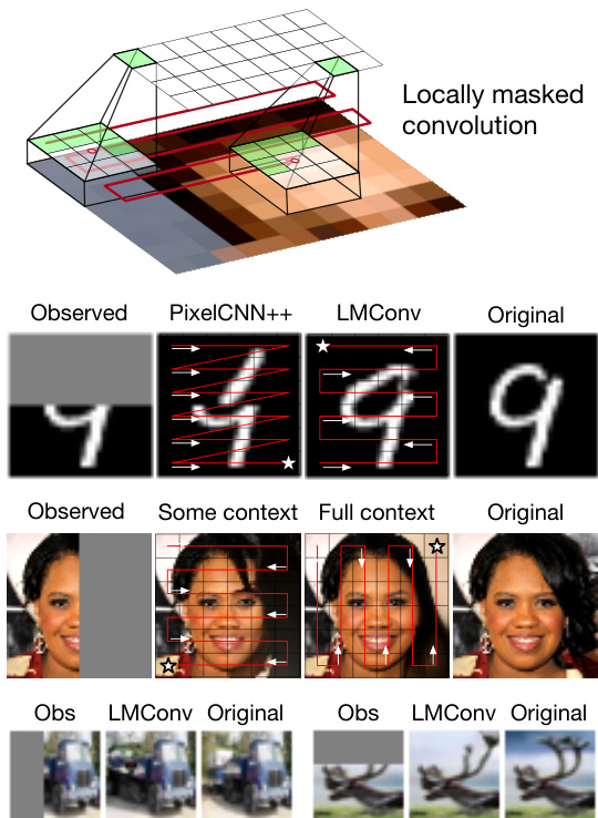
Figure 1: The ideal auto regressive joint distribution decomposition and sampling order are task-dependent. We learn to generate images under multiple orderings with the same parameters via locally masked convolutions (top), enabling global coherence for image completion (bottom).
图 1: 理想的自回归联合分布分解与采样顺序取决于具体任务。我们通过局部掩码卷积 (top) 学习用相同参数生成多种顺序的图像,实现图像补全的全局一致性 (bottom)。
1 INTRODUCTION
1 引言
Learning generative models of high-dimensional data such as images is a holy grail of machine learning with pervasive applications. Significant progress on this problem would naturally lead to a wide range of applications, including multimedia generation, compression, probabilistic time series forecasting, representation learning, and missing data completion. Many generative modeling frameworks have been proposed. Current state-of-the
学习生成高维数据(如图像)的模型是机器学习领域的圣杯,具有广泛的应用前景。该问题的重大突破自然将带来多媒体生成、压缩、概率时间序列预测、表征学习以及缺失数据补全等众多应用。目前已提出多种生成建模框架。当前最先进的...
Proceedings of the $36^{t h}$ Conference on Uncertainty in Artificial Intelligence (UAI), PMLR volume 124, 2020.
第36届人工智能不确定性会议论文集(UAI),PMLR第124卷,2020年。
art models for high-dimensional image data include (a) auto regressive models (Bengio and Bengio, 2000; Efros and Leung, 1999), (b) normalizing flow density estimators (Rezende and Mohamed, 2015), (c) generative adversarial networks (GANs) (Goodfellow et al., 2014), (d) latent variable models such as the VAE (Kingma and Welling, 2014; Rezende et al., 2014) and (e) energybased models e.g. Hinton (2002); LeCun et al. (2006); Du and Mordatch (2019); Song and Ermon (2019). While GANs, VAEs and EBMs have had great success in highdimensional image generation, exact likelihoods are generally intractable. Likelihood estimation is key for many practical applications from uncertainty estimation, robustness, reliability and safety perspectives. In contrast, auto regressive and flow models estimate exact likelihoods and can be used for uncertainty estimation, though still have room for improved generation quality. In this work, our focus is on auto regressive models.
高维图像数据的生成模型包括:(a) 自回归模型 (Bengio and Bengio, 2000; Efros and Leung, 1999)、(b) 归一化流密度估计器 (Rezende and Mohamed, 2015)、(c) 生成对抗网络 (GAN) (Goodfellow et al., 2014)、(d) 变分自编码器 (VAE) 等潜变量模型 (Kingma and Welling, 2014; Rezende et al., 2014) 以及 (e) 基于能量的模型 (Hinton, 2002; LeCun et al., 2006; Du and Mordatch, 2019; Song and Ermon, 2019)。虽然 GAN、VAE 和基于能量的模型在高维图像生成方面取得了巨大成功,但精确似然通常难以计算。从不确定性估计、鲁棒性、可靠性和安全性的角度来看,似然估计是许多实际应用的关键。相比之下,自回归模型和流模型可以估计精确似然并用于不确定性估计,尽管生成质量仍有提升空间。本工作的重点是自回归模型。
Given $n$ variables, one can generate $n!$ auto regressive decompositions of the joint likelihood, each corresponding to a forward sampling order, and more if we assume conditional independence. Early auto regressive texture synthesis (Popat and Picard, 1993; Efros and Leung, 1999) work could support multiple orders. However, recent CNN-based auto regressive models for images (van den Oord et al., 2016b,a; Salimans et al., 2017) capture only one of these orders (typically left-to-right raster scan, Fig. 2) for practical computational efficiency. Training and testing with a single order will not support all scenarios. Consider the image completion task in first row of Figure 1. If the top half of the image is missing, a raster scan generation order from left-to-right and top-to-bottom does not allow the model to condition on the context given in the observed bottom half of the image as the required conditionals are not estimated by the model.
给定 $n$ 个变量,可以生成 $n!$ 种联合似然的自回归分解,每种对应一种前向采样顺序,如果假设条件独立,则会有更多分解。早期的自回归纹理合成 (Popat and Picard, 1993; Efros and Leung, 1999) 工作支持多种顺序。然而,近期基于 CNN 的图像自回归模型 (van den Oord et al., 2016b,a; Salimans et al., 2017) 出于实际计算效率考虑,仅捕获其中一种顺序(通常是左至右的光栅扫描,图 2)。使用单一顺序进行训练和测试无法支持所有场景。以图 1 第一行的图像补全任务为例:若图像上半部分缺失,从左至右、从上至下的光栅扫描生成顺序无法让模型基于图像下半部观察到的上下文进行条件生成,因为模型并未估计所需的条件概率。
In this work, we propose a scalable, yet simple modification to convolutional auto regressive models to estimate more accurate likelihoods with a minor change in computation during training. Our goal is to support arbitrary orders in a scalable manner, allowing more precise likelihoods by averaging over several graphical models corresponding to orders (a form of Bayesian model averaging). Some past works have supported arbitrary orders in auto regressive models by learning separate parameters for each model (Frey, 1998), or by masking the input image to hide successor variables (Larochelle and Murray, 2011). A more efficient approach is to estimate densities in parallel across dimensions by masking network weights (Germain et al., 2015) differently for each order. However, all these methods are still computationally inefficient and difficult to scale beyond fully-connected networks to convolutional architectures.
在本工作中,我们提出了一种可扩展且简单的卷积自回归模型改进方法,通过微调训练计算过程来获得更精确的似然估计。我们的目标是以可扩展方式支持任意顺序,通过平均对应不同顺序的多个图模型(一种贝叶斯模型平均形式)来提升似然估计精度。先前研究曾通过为每个模型学习独立参数 (Frey, 1998) 或通过掩码输入图像隐藏后续变量 (Larochelle and Murray, 2011) 来实现自回归模型的任意顺序支持。更高效的方法是针对不同顺序差异化地掩码网络权重 (Germain et al., 2015),实现跨维度的并行密度估计。然而,这些方法仍存在计算效率低下的问题,且难以从全连接网络扩展到卷积架构。
In this work, we perform order-agnostic distribution estimation for natural images with state-of-the-art convolutional architectures. We propose to support arbitrary orderings by introducing masking at the level of features, rather than on inputs or weights. We show how an autoregressive CNN can support and learn multiple orders, with a single set of weights, via locally masked convolutions that efficiently apply location-specific masks to patches of each feature map. These local convolutions can be efficiently implemented purely via matrix multiplication by incorporating masking at the level of the im2col and col2im separation of convolution (Jia et al., 2014).
在本工作中,我们采用最先进的卷积架构对自然图像进行顺序无关的分布估计。我们提出通过在特征层面(而非输入或权重)引入掩码机制来支持任意排序方式。研究表明,自回归CNN可通过局部掩码卷积(使用单一权重集)支持并学习多种顺序模式,该技术能高效地对每个特征图区块施加位置特异性掩码。这些局部卷积可通过在im2col和col2im卷积分离阶段(Jia et al., 2014)整合掩码操作,完全基于矩阵乘法实现高效运算。
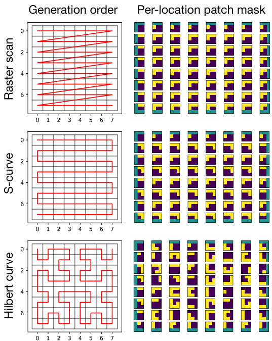
Figure 2: The three pixel generation orders and corresponding local masks that we consider in this work.
图 2: 本研究中考虑的三种像素生成顺序及对应局部掩码。
Arbitrary orders allow us to customize the traversal based on the needs of the task, which we evaluate in experiments. For instance, consider the examples shown in Fig. 1. The flexibility allows us to select the sampling order that exposes the maximum possible context for image completion, choose orderings that eliminate blind-spots (unobservable pixels) in image generation, and ensemble across multiple orderings using the same network weights. Note that such a model is able to support these image completions without training on any inpainting masks.
任意顺序允许我们根据任务需求自定义遍历方式,我们将在实验中对此进行评估。例如,考虑图 1 所示的示例。这种灵活性使我们能够选择在图像补全中暴露最大可能上下文的采样顺序,消除图像生成中盲点(不可观察像素)的排序方式,并使用相同的网络权重在多种排序中进行集成。值得注意的是,这样的模型无需在任何修复掩码上进行训练即可支持这些图像补全任务。
In experiments, we show that our approach can be efficiently implemented and is flexible without sacrificing the overall distribution estimation performance. By introducing order-agnostic training via LMCONV, we significantly outperform $\mathrm{PixelCNN{++}}$ on the unconditional CIFAR10 dataset, achieving code lengths of 2.89 bits per dimension. We show that the model can generalize to some novel orders. Finally, we significantly outperform raster-scan baselines on conditional likelihoods relevant to image completion by customizing the generation order.
实验中,我们证明该方法能高效实现且保持灵活性,同时不牺牲整体分布估计性能。通过LMCONV引入顺序无关训练,我们在无条件CIFAR10数据集上以2.89比特/维度的编码长度显著超越$\mathrm{PixelCNN{++}}$。结果表明模型可泛化至某些新顺序。最后,通过定制生成顺序,我们在图像补全相关条件似然任务上显著优于光栅扫描基线。
2 BACKGROUND
2 背景
Deep auto regressive models estimate high-dimensional data distributions using samples from the joint distribution over D-dimensions $p_{\mathtt{d a t a}}(\mathbf{x}{1},\dots,\mathbf{x}{D})$ . In this set- ting, we wish to approximate the joint with a parametric model $p_{\theta}(\mathbf{x}{1},\ldots,\mathbf{x}{D})$ by minimizing KL-divergence $D_{K L}(p_{\mathrm{data}}||p_{\theta})$ , or equivalently by maximizing the loglikelihood of the samples. As a general modeling principle, we can divide high-dimensional variables into many low-dimensional parts such as single dimensions, and capture dependencies between dimensions with a directed graphical model. Following the notation of (Kingma et al., 2019), these auto regressive (AR) models represent the joint distribution as a product of conditionals,
深度自回归模型利用来自D维联合分布$p_{\mathtt{data}}(\mathbf{x}{1},\dots,\mathbf{x}{D})$的样本来估计高维数据分布。在此设定下,我们希望通过最小化KL散度$D_{KL}(p_{\mathrm{data}}||p_{\theta})$(或等价地最大化样本对数似然)来用参数化模型$p_{\theta}(\mathbf{x}{1},\ldots,\mathbf{x}_{D})$近似联合分布。根据通用建模原则,可将高维变量分解为多个低维部分(如单维度),并通过有向图模型捕捉维度间依赖关系。沿用(Kingma等人, 2019)的符号表示,这类自回归(AR)模型将联合分布表示为条件概率的乘积:
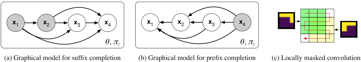
Figure 3: (a) A graphical model where the final, unobserved variables $x_{3},x_{4}$ can be efficiently completed via forward sampling conditioned on the observed variables $x_{1},x_{2}$ . (b) When $x_{4}$ is observed, we sample $x_{1},x_{2}$ , and $x_{3}$ in the second graphical model using the same parameters. (c) LMCONV defines the model with masks at each filter location.
图 3: (a) 一个概率图模型,其中最终未观测变量 $x_{3},x_{4}$ 可通过基于观测变量 $x_{1},x_{2}$ 的前向采样高效补全。(b) 当 $x_{4}$ 被观测时,我们在第二个概率图模型中使用相同参数对 $x_{1},x_{2}$ 和 $x_{3}$ 进行采样。(c) LMCONV 通过在每个滤波器位置定义掩码来构建模型。
$$
\begin{array}{l}{{\displaystyle p_{\theta}({\bf x})=p_{\theta}(x_{1},\ldots,x_{D})}}\ {{\displaystyle\quad=p_{\theta}(x_{\pi(1)})\prod_{i=2}^{D}p_{\theta}\left(x_{\pi(i)}\mid{\cal P}a({\bf x}_{\pi(i)})\right)}}\end{array}
$$
$$
\begin{array}{l}{{\displaystyle p_{\theta}({\bf x})=p_{\theta}(x_{1},\ldots,x_{D})}}\ {{\displaystyle\quad=p_{\theta}(x_{\pi(1)})\prod_{i=2}^{D}p_{\theta}\left(x_{\pi(i)}\mid{\cal P}a({\bf x}_{\pi(i)})\right)}}\end{array}
$$
where $\pi:[D]\to[D]$ is a permutation defining an order over the dimensions, $P a(\mathbf{x}{\pi(i)})=\mathbf{x}{\pi(1)},\ldots,\mathbf{x}{\pi(i-1)}$ defines the parents of $x_{\pi(i)}$ in the graphical model, and $\theta$ is a parameter vector. As any joint can be decomposed in this manner according to the product rule, this factorization provides the foundation for many models including ours. The primary challenge in auto regressive models is defining a sufficiently expressive family for the conditionals where parameter estimation is efficient. Deep autoregressive models parameter ize the conditionals with a neural network that is provided the context $P a(\mathbf{x}_{\pi(i)})$ .
其中 $\pi:[D]\to[D]$ 是一个定义维度顺序的排列,$P a(\mathbf{x}{\pi(i)})=\mathbf{x}{\pi(1)},\ldots,\mathbf{x}{\pi(i-1)}$ 定义了图模型中 $x_{\pi(i)}$ 的父节点,$\theta$ 是参数向量。由于任何联合分布都可以根据乘积规则以这种方式分解,这种分解为包括我们模型在内的许多模型奠定了基础。自回归模型的主要挑战是为条件分布定义一个表达能力足够强且参数估计高效的族。深度自回归模型通过神经网络对条件分布进行参数化,该网络接收上下文 $P a(\mathbf{x}_{\pi(i)})$。
Decomposition (1) converts the joint modeling problem into a sequence modeling problem. Forward (ancestral) sampling draws root variable $x_{\pi(1)}$ first, then samples the remaining dimensions in order $x_{\pi(2)},\ldots,x_{\pi(D)}$ from their respective conditionals. Given a particular autoregressive decomposition of the joint, forward sampling supports a single data generation order. The joint model density for an observed variable can be computed exactly by evaluating each conditional, allowing density estimation and maximum likelihood parameter estimation,
分解 (1) 将联合建模问题转化为序列建模问题。前向 (祖先) 采样首先抽取根变量 $x_{\pi(1)}$ ,然后按顺序 $x_{\pi(2)},\ldots,x_{\pi(D)}$ 从各自的条件分布中采样剩余维度。给定联合分布的特定自回归分解形式时,前向采样仅支持单一数据生成顺序。通过评估每个条件分布,可精确计算观测变量的联合模型密度,从而实现密度估计和最大似然参数估计。

With some choices of network architecture, the conditionals can be computed in parallel by masking weights (Germain et al., 2015; van den Oord et al., 2016b). In the PixelCNN model family, masked convolutions are causal: the features output by a masked convolution can only depend on features earlier in the order.
在某些网络架构的选择下,可以通过掩码权重并行计算条件概率 (Germain et al., 2015; van den Oord et al., 2016b)。在PixelCNN模型系列中,掩码卷积具有因果性:掩码卷积输出的特征只能依赖于顺序中较早的特征。
While the choice of order is arbitrary, temporal and sequential data modalities have a natural ordering from the first dimension in the sequence to the last. For spatial data such as images, a natural ordering is not clear. For computational reasons, a raster scan order is generally used where the top left pixel is modeled unconditionally and generation proceeds in row-major fashion across each row from left to right, depicted in Figure 1, second column.
虽然顺序的选择是任意的,但时间和序列数据模态具有从序列的第一个维度到最后一个维度的自然排序。对于图像等空间数据,自然排序并不明确。出于计算原因,通常采用光栅扫描顺序,即左上角像素无条件建模,生成过程按行主序从左到右逐行进行,如图1第二列所示。
3 IMAGE COMPLETION WITH MAXIMUM RECEPTIVE FIELD
3 最大感受野的图像补全
For estimating the distribution of 2D images, a raster scan ordering is perhaps as good of an order as any other choice. That said, the raster scan order has necessitated architectural innovations to allow the neural network to access information far back in the sequence such as twodimensional PixelRNNs (van den Oord et al., 2016b), two- stream shift-based convolutional architectures (van den Oord et al., 2016a), and self-attention combined with convolution (Chen et al., 2018). These structures significantly improve test-set likelihoods and sample quality, but marry network architectures to the raster scan order.
在估计二维图像的分布时,栅格扫描顺序可能与其他选择一样合适。然而,栅格扫描顺序需要架构创新,以使神经网络能够访问序列中较远的信息,例如二维PixelRNN (van den Oord et al., 2016b)、基于双流位移的卷积架构 (van den Oord et al., 2016a),以及卷积与自注意力结合的方法 (Chen et al., 2018)。这些结构显著提高了测试集似然和样本质量,但也将网络架构与栅格扫描顺序紧密绑定。
Fixing a particular order is limiting for missing data completion tasks. Letting $\pi(i)=i$ denote the raster scan order, PixelRNN and PixelCNN architectures can complete only the bottom part of the image via forward sampling: given observations $x_{1},\ldots,x_{d}$ , raster scan auto regressive models sequentially sample,
固定特定顺序对缺失数据补全任务具有限制性。令 $\pi(i)=i$ 表示光栅扫描顺序时,PixelRNN和PixelCNN架构仅能通过前向采样完成图像底部区域:给定观测值 $x_{1},\ldots,x_{d}$ 后,光栅扫描自回归模型会依次采样

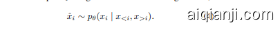
If all dimensions other than $x_{i}$ are observed, ideally we would sample $\hat{x}_{i}$ using maximum conditioning context,
如果除 $x_{i}$ 外的所有维度都被观测到,理想情况下我们会使用最大条件上下文对 $\hat{x}_{i}$ 进行采样。
Unfortunately, the raster scan model only predicts distributions of the form $p_{\theta}(x_{i}\mid x_{<i})$ , and ignores observations $x_{>i}$ during completion. In the worst case, a model with a raster scan generation order cannot observe any of the context for an inpainting task where the top half of the image is unknown (Figure 1, $\mathrm{PixelCNN{++}}$ ). This leads to image completions that do not respect global structure. Small numbers of dimensions could be sampled by computing the posterior, e.g. for $i=1$ ,
遗憾的是,光栅扫描模型仅能预测形式为 $p_{\theta}(x_{i}\mid x_{<i})$ 的分布,且在补全过程中会忽略观测值 $x_{>i}$。最坏情况下,对于图像上半部分未知的修复任务(图1:$\mathrm{PixelCNN{++}}$),采用光栅扫描生成顺序的模型将无法观察到任何上下文信息。这会导致图像补全结果与全局结构不符。虽然可以通过计算后验分布来采样少量维度(例如 $i=1$ 时),

but this is expensive as each summand requires neural network evaluation, and becomes intractable when several dimensions are unknown. Instead of approximating the posterior, we estimate parameters $\theta$ that achieve high likelihood with multiple auto regressive decomposition s,
但这种方法成本高昂,因为每个求和项都需要进行神经网络评估,且在多个维度未知时会变得难以处理。我们不再近似后验分布,而是通过多重自回归分解来估计能实现高似然度的参数$\theta$。

with $p_{\pi}$ denoting a uniform distribution over several orderings. The joint distribution under $\pi$ factorizes according to (1). The resulting conditionals are all parameterized by the same neural network. By choosing order prior $p_{\pi}$ that supports a $\pi$ such that $\pi(D)=i$ , we can use the network with such an ordering to query (4) directly.
其中 $p_{\pi}$ 表示对几种排序的均匀分布。$\pi$ 下的联合分布根据 (1) 式进行分解。最终的条件分布均由同一个神经网络参数化。通过选择支持 $\pi(D)=i$ 的排序先验 $p_{\pi}$,我们可以直接使用具有此类排序的网络来查询 (4)。
During optimization with stochastic gradient descent, we make single-sample estimates of the inner expectation in (6) according to order-agnostic training (Uria et al., 2014; Germain et al., 2015), using a single order per batch.
在使用随机梯度下降进行优化时,我们根据与顺序无关的训练方法 (Uria et al., 2014; Germain et al., 2015),对(6)式中的内部期望进行单样本估计,每个批次仅使用单一顺序。
For a test-time task where ${x_{i}:i\in T_{\mathrm{obs}}}$ are observed, we select a $\pi$ that the model was trained with such that
对于一个测试时任务,其中观测到 ${x_{i}:i\in T_{\mathrm{obs}}}$,我们选择模型训练时使用的 $\pi$ 使得
$$
{\pi(1),\ldots,\pi(|T_{\mathrm{obs}}|)}=T_{\mathrm{obs}},
$$
$$
{\pi(1),\ldots,\pi(|T_{\mathrm{obs}}|)}=T_{\mathrm{obs}},
$$
i.e. the first $|T_{\mathrm{obs}}|$ dimensions in the generation order are the observed dimensions, then sample according to the rest of the order so that the model posterior over each unknown dimension is conditioned either on observed or previously sampled dimensions.
即在生成顺序中前 $|T_{\mathrm{obs}}|$ 个维度为观测维度,随后按照剩余顺序进行采样,使得模型对每个未知维度的后验分布均以已观测或先前采样的维度为条件。
4 LOCAL MASKING
4 局部掩码
In this section, we develop locally masked convolutions (LMCONV): a modification to the standard convolution operator that allows control over generation order and parallel computation of conditionals for evaluating likelihood. In the first convolutional layer of a neural network, $C_{\mathrm{out}}$ filters of size $k\times k$ are applied to the input image with spatial invariance: the same parameters are used at all locations in a sliding window. Each filter has $k^{2}*C_{\mathrm{in}}$ parameters. For images with disc ret i zed intensities, convolutional auto regressive networks transform a spatial $H\times W$ , multi-channel image into a tensor of log-probabilities that define the conditional distributions of (1). These log-probabilities take the form of an $H\times W$ image, with channel count equal to the number of color channels times the number of bins per color channel. The output log-probabilities at coordinate $i,j$ in the output define the distribution $p_{\theta}(x_{i,j}\mid P a(p(x_{i,j}))$ . Critically, this distribution must not depend on observations of successors in the Bayesian network, or the product of conditionals will not define a valid distribution due to cyclicity.
在本节中,我们提出了局部掩码卷积 (LMCONV):一种对标准卷积算子的改进,能够控制生成顺序并并行计算条件概率以评估似然。在神经网络的第一个卷积层中,会将 $C_{\mathrm{out}}$ 个尺寸为 $k\times k$ 的滤波器以空间不变性的方式应用于输入图像:在滑动窗口的所有位置使用相同的参数。每个滤波器具有 $k^{2}*C_{\mathrm{in}}$ 个参数。对于具有离散化强度的图像,卷积自回归网络将空间尺寸为 $H\times W$ 的多通道图像转换为对数概率张量,这些对数概率定义了(1)式的条件分布。这些对数概率的形式为 $H\times W$ 的图像,其通道数等于颜色通道数乘以每个颜色通道的分箱数。输出中坐标 $i,j$ 处的输出对数概率定义了分布 $p_{\theta}(x_{i,j}\mid P a(p(x_{i,j}))$ 。关键的是,该分布不能依赖于贝叶斯网络中后继节点的观测值,否则由于循环性,条件概率的乘积将无法定义有效分布。
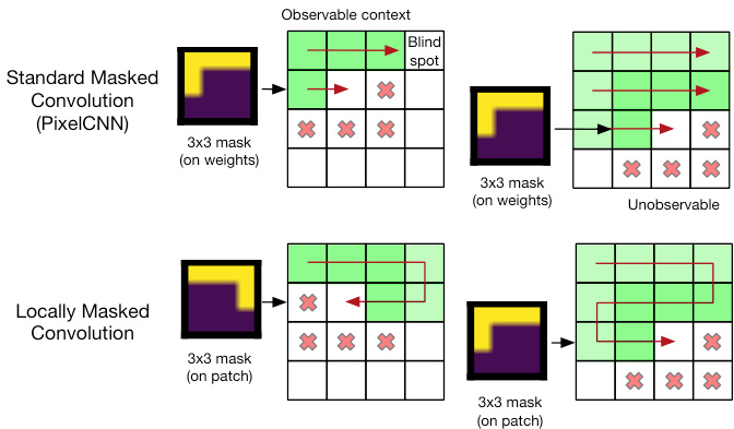
Figure 4: A comparison of standard weight masked convolutions and the proposed locally masked convolution.
图 4: 标准权重掩码卷积与提出的局部掩码卷积对比。
NADE (Larochelle and Murray, 2011) circumvents the problem by masking the input image, though requires independent forward passes to compute each factor of the auto regressive decomposition (1). Instead, the PixelCNN model family controls information flow through the network by setting certain weights of the convolution filters to zero, similar to how MADE (Germain et al., 2015) masks the weight matrices in fully-connected layers. We depict masked convolutions for the first convolutional layer in Figure 4. As a single mask is applied to the $C_{\mathrm{in}}\times k\times k$ parameter tensor defining each convolutional filter, the same masking pattern is applied at all locations in the image. Sharing the masking pattern constrains the possible orders, and leads to blind spots which the output distribution is unable to observe.
NADE (Larochelle and Murray, 2011) 通过掩码输入图像规避了该问题,但需要独立前向传递来计算自回归分解 (1) 的每个因子。相比之下,PixelCNN 模型家族通过将卷积滤波器的特定权重设为零来控制信息流,类似于 MADE (Germain et al., 2015) 在全连接层中掩码权重矩阵的方式。我们在图 4 中展示了第一卷积层的掩码卷积操作。由于每个卷积滤波器的 $C_{\mathrm{in}}\times k\times k$ 参数张量采用单一掩码模式,该掩码模式会作用于图像所有位置。共享掩码模式会限制可能的顺序关系,并导致输出分布无法观测到的盲区。
In practice, convolutions are implemented through general matrix multiplication (GEMM) due to widely available, heavily optimized and parallel i zed implementations of the operation on GPU and CPU. To use matrix multiplication, the input to a layer is rearranged in memory via the $\mathrm{im}2\mathrm{col}$ algorithm, which extracts $C_{\mathrm{in}}\times k\times k$ patches from the $C_{\mathrm{in}}\times H\times W$ input at each location that a convolutional filter will be applied. Assuming padding and a stride of 1 is used, the rearrangement yields matrix $X$ with $C_{\mathrm{in}}k^{2}$ rows and $HW$ columns. To perform convolution, the framework left-multiplies weight matrix $\mathcal{W}$ , storing $Y=\mathcal{W}X$ , adds a bias, and finally rearranges $Y$ into a spatial format via the col2im algorithm.
实践中,由于GPU和CPU上广泛提供且经过高度优化并行化的通用矩阵乘法(GEMM)实现,卷积运算通常通过GEMM来完成。为了使用矩阵乘法,层的输入会通过$\mathrm{im}2\mathrm{col}$算法在内存中重新排列,该算法从$C_{\mathrm{in}}\times H\times W$的输入中提取每个卷积滤波器将应用位置的$C_{\mathrm{in}}\times k\times k$补丁。假设使用填充且步长为1,重排后得到具有$C_{\mathrm{in}}k^{2}$行和$HW$列的矩阵$X$。执行卷积时,框架会左乘权重矩阵$\mathcal{W}$,存储$Y=\mathcal{W}X$,添加偏置,最后通过col2im算法将$Y$重新排列为空间格式。
We exploit this data rearrangement to arbitrarily mask the input to the convolutional filter at each location it is
我们利用这种数据重排方式,在卷积滤波器每个位置处对输入进行任意掩码处理
applied. The inputs to the convolution at each location, i.e. the input patches, form columns of $X$ . For a given generation order, we construct mask matrix $\mathcal{M}$ of the same dimensions as $X$ and set $X=\mathcal{M}\odot X$ prior to matrix multiplication. In particular, our locally masked convolution masks patches of the input to each layer, rather than masking weights and rather than masking the initial input to the network. LMCONV combines the flexibility of NADE and the parallel iz ability of MADE and PixelCNN. The LMCONV algorithm is summarized in Algorithm 1, and mask construction is detailed in Algorithm 2.
应用。在每个位置进行卷积的输入,即输入补丁,构成矩阵$X$的列。对于给定的生成顺序,我们构建与$X$维度相同的掩码矩阵$\mathcal{M}$,并在矩阵乘法前设置$X=\mathcal{M}\odot X$。具体而言,我们的局部掩码卷积是对每一层的输入补丁进行掩码,而不是对权重或网络的初始输入进行掩码。LMCONV结合了NADE的灵活性与MADE和PixelCNN的并行化能力。LMCONV算法总结在算法1中,掩码构造细节详见算法2。
We implement two versions of the layer with the PyTorch machine learning framework (Paszke et al., 2019). The first is an implementation that uses auto differentiation to compute gradients. As only the forward pass is defined by the user, the implementation is under 20 lines of Python.
我们基于PyTorch机器学习框架(Paszke等人,2019)实现了该层的两个版本。第一种是使用自动微分计算梯度的实现。由于用户仅需定义前向传播,该实现仅需不到20行Python语言代码。
However, reverse-mode auto differentiation incurs significant memory overheads during back propagation as the output of nearly every operation during the forward pass must be stored until gradient computation (Griewank and Walther, 2000; Jain et al., 2020). Data rearrangement with $\mathrm{im}2\mathrm{col}$ is memory intensive as features patches overlap and are duplicated. We implement a custom, memory efficient backward pass that only stores the input, the mask and the output of the layer during the forward pass and recomputes the $\mathrm{im}2\mathrm{col}$ operation during the backward pass. Re computing the im2col operation achieves $2.7\times$ memory savings at a $1.3\times$ slowdown.
然而,反向模式自动微分在反向传播过程中会产生显著的内存开销,因为前向传播阶段几乎所有操作的输出都必须存储到梯度计算时 (Griewank and Walther, 2000; Jain et al., 2020)。使用 $\mathrm{im}2\mathrm{col}$ 进行数据重排时,由于特征块重叠和重复,内存消耗巨大。我们实现了一种定制化的高效内存反向传播方案,在前向传播阶段仅存储该层的输入、掩码和输出,并在反向传播阶段重新计算 $\mathrm{im}2\mathrm{col}$ 操作。通过重新计算 im2col 操作,我们实现了 $2.7\times$ 的内存节省,代价是 $1.3\times$ 的速度下降。
Using locally masked convolutions, we can experiment with many different image generation orders. In this work, we consider three classes of orderings: raster scan, implemented in baseline PixelCNNs, an S-curve order that traverses rows in alternating directions, and a Hilbert space-filling curve order that generates nearby pixels in the image consecutively. Alternate orderings provide several benefits. Nearby pixels in an image are highly correlated. By generating these pixels close in a Hilbert curve order, we might expect information to propagate from the most important, nearby observations for each dimension and reduce the vanishing gradient problem.
通过使用局部掩码卷积,我们可以尝试多种不同的图像生成顺序。在本研究中,我们考虑了三种顺序类型:基线PixelCNN中实现的栅格扫描顺序、交替方向遍历行的S形曲线顺序,以及连续生成图像中相邻像素的希尔伯特空间填充曲线顺序。这些替代顺序具有多重优势:图像中的相邻像素具有高度相关性。通过采用希尔伯特曲线顺序近距离生成这些像素,我们可以期望信息从每个维度最重要、最邻近的观测点传播,从而缓解梯度消失问题。
If the image is considered a graph with nodes for each pixel and edges connecting adjacent pixels, a convolutional auto regressive model using an order defined by a Hamiltonian path over the image graph will also suffer no blind spot in a $D$ layer network. To see this, note that the features corresponding to dimension $x_{\pi(i)}$ in the Hamiltonian path order will always be able to observe the previous layer’s features corresponding to $x_{\pi(i-1)}$ . After at least $D$ layers of depth, the features for $x_{\pi(i)}$ will incorporate information from all $i-1$ previous dimensions. In practice, information propagates with fewer required layers in these architectures as multiple neighbors are observed in each layer. Finally, we select multiple orderings at inference and average the resulting joint distributions to compute better likelihood estimates.
如果将图像视为一个图,其中每个像素为节点,相邻像素间通过边连接,那么使用由图像图上的哈密尔顿路径定义的顺序的卷积自回归模型,在$D$层网络中也同样不会存在盲点。这是因为按照哈密尔顿路径顺序,维度$x_{\pi(i)}$对应的特征总能观察到上一层$x_{\pi(i-1)}$对应的特征。在至少$D$层深度后,$x_{\pi(i)}$的特征将整合来自前$i-1$个维度的所有信息。实际应用中,由于每层观察多个相邻节点,信息传播所需的层数更少。最后,在推理时我们选择多种顺序并对所得联合分布取平均,以计算更优的似然估计。
5 ARCHITECTURE
5 架构
We use a network architecture similar to $\mathrm{PixelCNN{++}}$ (Salimans et al., 2017), the best-in-class density estimator in the fully convolutional auto regressive PixelCNN model family. Convolution operations are masked according to Algorithm 1. While our locally masked convolutions can benefit from self-attention mechanisms used in later work, we choose a fully convolutional architecture for simplicity and to study the benefit of local masking in isolation of other architectural innovations. We make three modifications to the $\mathrm{PixelCNN{++}}$ architecture that simplify it and allow for arbitrary generation orders. Gated PixelCNN uses a two-stream architecture composed of two network stacks with $\textstyle\left\lfloor{\frac{k}{2}}\right\rfloor\times1$ and $\textstyle\left\lfloor{\frac{k}{2}}\right\rfloor\times k$ convolutions to enforce the raster scan order. In the horizontal stream, Gated PixelCNN applies non-square convolutions and feature map shifts or pads to extract information within the same row, to the left of the current dimension. In the vertical stream, Gated PixelCNN extracts information from above. Skip connections between streams allow information to propagate. $\mathrm{PixelCNN{++}}$ uses a similar architecture based on a U-Net (Ronne berger et al., 2015) with approximately 54M parameters. We replace the two streams with a simple, single stream with the same depth, using LMCONV to maintain the auto regressive property. Masks for these convolutions are computed and cached at the beginning of training. Due to the regularizing effect of order-agnostic training, we do not use dropout.
我们采用与$\mathrm{PixelCNN{++}}$ (Salimans等人,2017)相似的网络架构,这是全卷积自回归PixelCNN模型家族中最先进的密度估计器。卷积操作根据算法1进行掩码处理。虽然我们的局部掩码卷积可以从后续工作中使用的自注意力机制中受益,但为了简化研究并单独考察局部掩码的效益,我们选择了全卷积架构。我们对$\mathrm{PixelCNN{++}}$架构进行了三处修改以简化结构并支持任意生成顺序。
门控PixelCNN采用双流架构,由两个网络堆栈组成,分别使用$\textstyle\left\lfloor{\frac{k}{2}}\right\rfloor\times1$和$\textstyle\left\lfloor{\frac{k}{2}}\right\rfloor\times k$卷积来强制光栅扫描顺序。在水平流中,门控PixelCNN通过非方形卷积和特征图移位/填充来提取同一行当前维度左侧的信息;在垂直流中则提取上方信息。流间的跳跃连接允许信息传播。$\mathrm{PixelCNN{++}}$采用基于U-Net (Ronneberger等人,2015)的类似架构,包含约5400万参数。我们将其替换为相同深度的单流结构,使用LMCONV保持自回归特性。这些卷积的掩码在训练开始时计算并缓存。由于顺序无关训练的正则化效果,我们未使用dropout。
Table 1: Average negative log likelihood of binarized and grayscale MNIST digits under our model. Lower is better.
| BINARIZEDMNIST,28x28 | NLL (nats) |
| DARN (Intractable) (Gregor et al., 2014) NADE (Uria et al.,2014) EoNADE 2hl (128orders)(Uriaet al.,2014) EoNADE-5 2hl (128 orders) (Raiko et al.,2014) | 84.13 88.33 85.10 84.68 86.64 |
| Ours,S-curve(1 order) Ours,S-curve(8orders) GRAYSCALEMNIST,28x28 | 78.47 77.58 |
| Spatial PixelCNN (Akoury and Nguyen, 2017) PixelCNN++(1 stream) Ours,S-curve(1 order) Ours,S-curve (8orders) | NLL (bpd) 0.88 0.77 0.68 |
表 1: 二值化和灰度 MNIST 数字在我们模型下的平均负对数似然。数值越低越好。
| BINARIZEDMNIST,28x28 | NLL (nats) |
|---|---|
| DARN (Intractable) (Gregor et al., 2014) NADE (Uria et al.,2014) EoNADE 2hl (128orders)(Uriaet al.,2014) EoNADE-5 2hl (128 orders) (Raiko et al.,2014) | 84.13 88.33 85.10 84.68 86.64 |
| Ours,S-curve(1 order) Ours,S-curve(8orders) GRAYSCALEMNIST,28x28 | 78.47 77.58 |
| Spatial PixelCNN (Akoury and Nguyen, 2017) PixelCNN++(1 stream) Ours,S-curve(1 order) Ours,S-curve (8orders) | NLL (bpd) 0.88 0.77 0.68 |
Second, we use dilated convolutions (Yu and Koltun, 2015) at regular intervals in the model rather than downsampling the feature map. Down sampling precludes many orders, as the operation aggregates information from contiguous squares of pixels together without a mask. Dilated convolutions expand the receptive field without limiting the order, as local masks can be customized to hide or reveal specific features accessed by the filter.
其次,我们在模型中定期使用空洞卷积 (dilated convolutions) (Yu and Koltun, 2015) ,而不是对特征图进行下采样。下采样会排除许多阶数,因为该操作在没有掩码的情况下将相邻像素块的信息聚合在一起。空洞卷积在不限制阶数的情况下扩展了感受野,因为可以自定义局部掩码来隐藏或显示滤波器访问的特定特征。
Finally, we normalize the feature map across the channel dimension (Li et al., 2019). Normalization allows masks to have varying numbers of ones at each spatial location by rescaling features to the same scale.
最后,我们在通道维度上对特征图进行归一化处理 (Li et al., 2019)。归一化通过将特征重新缩放到相同尺度,使得每个空间位置上的掩码可以拥有不同数量的激活值。
As in $\mathrm{PixelCNN{++}}$ , our model represents each conditional with a mixture of 10 disc ret i zed logistic distributions that imposes a distribution over binned pixel intensities. For the binarized MNIST dataset (Salak hut dino v and Murray, 2008), we instead use a softmax over two logits. We train with 8 variants of an S-curve (zig-zag) order that traverses each row of the image in alternating directions so that consecutively generated pixels are adjacent, and so that locally masked CNNs with sufficient depth can achieve the maximum allowed receptive field.
与 $\mathrm{PixelCNN{++}}$ 类似,我们的模型用10个离散化逻辑分布的混合表示每个条件,对分箱像素强度施加分布。对于二值化MNIST数据集 (Salak hut dino v and Murray, 2008),我们改用两个logits的softmax。训练时采用8种S形(锯齿形)扫描顺序变体,通过交替方向遍历图像的每一行,使得连续生成的像素相邻,且具有足够深度的局部掩码CNN能达到最大允许感受野。
Table 2: Average negative log likelihood of CIFAR10 images under our model. Lower is better.
| CIFAR10,32x32 | NLL (bpd) |
| UniformDistribution | 8.00 |
| Multivariate Gaussian(vanden Oord et al.,2016b) | 4.70 |
| Attention-based Image Transformer (Parmar et al.,2018) | 2.90 |
| PixelSNAIL(Chen et al.,2018) | 2.85 |
| Sparse Transformer (Child et al.,2019) | 2.80 |
| Convolutional | |
| PixelCNN (1 stream)(van den Oord et al.,2016b) | 3.14 |
| Gated PixelCNN (2 stream)(van den Oord et al.,2016a) | 3.03 |
| PixelCNN++(1 stream) | |
| PixelCNN++(2 stream)(Salimans et al.,2017) | 2.99 |
| 2.92 | |
| Ours,S-curve(1 stream,1 order) Ours,S-curve(1 stream,8 orders) | 2.91 |
表 2: 我们的模型在CIFAR10图像上的平均负对数似然。数值越低越好。
| CIFAR10,32x32 | NLL (bpd) |
|---|---|
| UniformDistribution | 8.00 |
| Multivariate Gaussian (van den Oord et al., 2016b) | 4.70 |
| Attention-based Image Transformer (Parmar et al., 2018) | 2.90 |
| PixelSNAIL (Chen et al., 2018) | 2.85 |
| Sparse Transformer (Child et al., 2019) | 2.80 |
| Convolutional | |
| PixelCNN (1 stream) (van den Oord et al., 2016b) | 3.14 |
| Gated PixelCNN (2 stream) (van den Oord et al., 2016a) | 3.03 |
| PixelCNN++ (1 stream) | |
| PixelCNN++ (2 stream) (Salimans et al., 2017) | 2.99 |
| 2.92 | |
| Ours, S-curve (1 stream, 1 order) Ours, S-curve (1 stream, 8 orders) | 2.91 |
Across all quantitative experiments, we use a model with approximately 46M parameters, trained with the Adam optimizer with a learning rate of $210^{-4}$ decayed by a factor of $1-510^{-6}$ per iteration with clipped gradients. For CelebA-HQ qualitative results, we increase filter count and train a model with 184M parameters. More details are provided in the appendix.
在所有定量实验中,我们使用了一个约4600万参数的模型,采用Adam优化器进行训练,初始学习率为$210^{-4}$,每迭代一次衰减$1-510^{-6}$因子,并采用梯度裁剪。针对CelebA-HQ的定性结果,我们增加了滤波器数量并训练了一个1.84亿参数的模型。更多细节见附录。
6 EXPERIMENTS
6 实验
To evaluate the benefits of our approach, we study three scientific questions: (1) do locally masked auto regressive ensembles estimate more accurate likelihoods on image datasets than single-order models?, (2) can the model generalize to novel orders? and (3) how important is order selection for image completion?
为了评估我们方法的优势,我们研究了三个科学问题:(1) 局部掩码自回归集成模型在图像数据集上的似然估计是否比单序模型更准确?(2) 该模型能否泛化到新序列?(3) 序列选择对图像补全有多重要?
We estimate the distribution of three image datasets: $28\times28$ grayscale and binary (Salak hut dino v and Murray, 2008) MNIST digits, $32\times32$ 8-bit color CIFAR10 natural images, and high-resolution CelebA-HQ 5-bit color face photographs (Karras et al., 2018). Unlike classification, density estimation remains challenging on these datasets. We train the CelebA-HQ models at $256\times256$ resolution to compare with prior density estimation work, and at a bilinearly down sampled $64\times64$ resolution.
我们评估了三个图像数据集的分布情况:$28\times28$ 灰度与二值化(Salak hut dino v and Murray, 2008)的MNIST手写数字、$32\times32$ 8位色CIFAR10自然图像,以及高分辨率5位色CelebA-HQ人脸照片(Karras et al., 2018)。与分类任务不同,这些数据集的密度估计仍具挑战性。为与先前密度估计研究对比,我们在$256\times256$分辨率下训练CelebA-HQ模型,同时采用双线性降采样至$64\times64$分辨率进行训练。
Our locally masked model achieves better likelihoods than PixelCNN $++$ by using multiple generation orders. We then show that the model can generalize to generation orders that it has not been trained with. Finally, for image completion, we achieve the best results over strong baselines by using orders that expose all observed pixels.
我们采用多生成顺序的局部掩码模型在似然度上优于PixelCNN++。实验表明,该模型能泛化至未训练过的生成顺序。最终在图像补全任务中,通过采用完全暴露观测像素的生成顺序,我们在强基线模型上取得了最佳效果。
Table 3: Average conditional negative log likelihood for Top, Left and Bottom half image completion.
| BINARIZEDMNIST28x28(nats) | T | L | B |
| Ours (adversarialorder) | 41.76 | 39.83 | 43.35 |
| Ours(1max contextorder) | 34.99 | 32.47 | 36.57 |
| Ours (2max context orders) | 34.82 | 32.25 | 36.36 |
| CIFAR1032x32(bpd) | T | L | B |
| PixelCNN++,1stream | 3.07 | 3.10 | 3.05 |
| PixelCNN++,2stream | 2.97 | 2.98 | 2.93 |
| Ours(1 stream,adversarial order) | 2.93 | 2.98 | 3.05 |
| Ours (1 stream,1 max context order) | 2.77 | 2.83 | 2.89 |
| Ours (1 stream,2max context orders) | 2.76 | 2.82 | 2.88 |
表 3: 顶部、左侧和底部半图像补全的平均条件负对数似然
| BINARIZEDMNIST28x28(nats) | T | L | B |
|---|---|---|---|
| Ours (adversarialorder) | 41.76 | 39.83 | 43.35 |
| Ours(1max contextorder) | 34.99 | 32.47 | 36.57 |
| Ours (2max context orders) | 34.82 | 32.25 | 36.36 |
| CIFAR1032x32(bpd) | T | L | B |
| PixelCNN++,1stream | 3.07 | 3.10 | 3.05 |
| PixelCNN++,2stream | 2.97 | 2.98 | 2.93 |
| Ours(1 stream,adversarial order) | 2.93 | 2.98 | 3.05 |
| Ours (1 stream,1 max context order) | 2.77 | 2.83 | 2.89 |
| Ours (1 stream,2max context orders) | 2.76 | 2.82 | 2.88 |
6.1 WHOLE-IMAGE DENSITY ESTIMATION
6.1 全图像密度估计
Tractable generative models are generally evaluated via the average negative log likelihood (NLL) of test data. For interpret ability, many papers normalize base 2 NLL by the number of dimensions. By normalizing, we can measure bits per dimension (bpd), or a lower-bound for the expected number of bits needed per pixel to losslessly compress images using a Huffman code with $p(\mathbf{x})$ estimated by our model. Better estimates of the distribution should result in higher compression rates. Tables 1 and 2 show likelihoods for our model and prior models.
可处理的生成模型通常通过测试数据的平均负对数似然 (NLL) 进行评估。为了便于解释,许多论文会按维度数对以 2 为底的 NLL 进行归一化。通过归一化,我们可以测量每维度比特数 (bpd),或使用霍夫曼编码无损压缩图像时每个像素所需比特数的期望下界,其中 $p(\mathbf{x})$ 由我们的模型估计。更好的分布估计应能带来更高的压缩率。表 1 和表 2 展示了我们的模型与先前模型的似然值。
On binarized MNIST (Table 1), our locally masked PixelCNN achieves significantly higher likelihoods (lower NLL) than baselines, including neural auto regressive models NADE, EoNADE, and MADE that average across large numbers of orderings. This is due to architectural advantages of our CNN and increased model capacity. Our model also outperforms the standard PixelCNN, which suffers from a blind spot problem due to sharing the same mask at all locations. Likelihood is further improved by using ensemble averaging across 8 orders that share parameters. These results are also observed on grayscale MNIST where each pixel has one of 256 intensity levels.
在二值化MNIST数据集(表1)上,我们提出的局部掩码PixelCNN模型在似然值(更低NLL)上显著优于包括NADE、EoNADE和MADE在内的神经自回归基线模型,这些基线模型通过对大量排序顺序进行平均来提升性能。这一优势源于我们CNN的架构改进和增强的模型容量。我们的模型也优于标准PixelCNN,后者因在所有位置使用相同掩码而存在盲点问题。通过采用8种参数共享排序顺序的集成平均方法,似然值得到了进一步提升。这些优势同样在256级灰度MNIST数据集上得到了验证。
On CIFAR10, we achieve 2.89 bpd test set likelihood when averaging the joint probability of 8 graphical models, each defined by an S-curve generation order. Our results outperform the state-of-the-art convolutional auto regressive model, PixelCNN $^{++}$ . We significantly outperform a 1 stream architectural variant of $\mathrm{PixelCNN{++}}$ that has the same number of parameters as our model and uses a similar architecture, differing only in that it uses a single raster scan order. By introducing order-agnostic ensemble averaging to convolutional auto regressive models, we combined the best of fully-connected density estimators that average over orders, and the inductive biases of CNNs. These results could further improve with selfattention mechanisms and additional capacity, which have been observed to improve the performance of singe-order estimation, marking an opportunity for future research.
在CIFAR10数据集上,我们通过平均8个图形模型的联合概率(每个模型由S曲线生成顺序定义)实现了2.89 bpd的测试集似然度。该结果超越了当前最先进的卷积自回归模型PixelCNN$^{++}$。我们显著优于$\mathrm{PixelCNN{++}}$的单流架构变体(该变体与我们的模型参数量相同且架构相似,仅采用单一光栅扫描顺序)。通过将顺序无关的集成平均方法引入卷积自回归模型,我们融合了全连接密度估计器(支持多顺序平均)与CNN归纳偏置的优势。结合自注意力机制和更大容量(这些改进已被证实能提升单顺序估计性能),未来研究有望取得更优结果。

Figure 5: CIFAR10 image completions using our locallymasked convolutions with a specialized ordering.
图 5: 使用我们具有专用排序的局部掩码卷积完成的CIFAR10图像补全。
Our model is also scalable to high resolution distribution estimation. On the CelebA-HQ 256x256 dataset at 5-bit color depth, our model achieves 0.74 bpd with a single Scurve order, outperforming Glow (Kingma and Dhariwal, 2018), an exact likelihood normalizing flow. In comparison, the state-of-the-art model, SPN (Menick and Kalchbrenner, 2019), achieves 0.61 bpd by using self-attention and a specialized architecture for high resolutions.
我们的模型同样具备高分辨率分布估计的可扩展性。在5位色深的CelebA-HQ 256x256数据集上,采用单一Scurve排序的模型实现了0.74 bpd,优于精确似然归一化流模型Glow (Kingma and Dhariwal, 2018)。相比之下,当前最先进的SPN模型 (Menick and Kalchbrenner, 2019) 通过使用自注意力机制和专为高分辨率设计的架构,达到了0.61 bpd。
6.2 GENERALIZATION TO NOVEL ORDERS
6.2 新顺序的泛化
Ideally, an order-agnostic model would be able to generate images in orders that it has not been trained with. To understand generalization to novel orders, we evaluate the test-set likelihood of a CIFAR10 model that achieves 2.93 bpd with a single S-curve order and 2.91 bpd with 8 S-curve orders under a raster scan decomposition. The model achieves 3.75 bpd with 1 raster scan order $28%$ increase) and 3.67 bpd with 8 raster scan orders $26%$ increase). While the novel order degrades compression rate, the model was trained with 8 fixed orders of the same S-curve type, which are fairly different from a raster scan.
理想情况下,一个与顺序无关的模型应该能够生成未经训练顺序的图像。为了理解对新顺序的泛化能力,我们评估了一个CIFAR10模型的测试集似然,该模型在单一S曲线顺序下达到2.93 bpd,在8种S曲线顺序下达到2.91 bpd(使用光栅扫描分解)。该模型在1种光栅扫描顺序下达到3.75 bpd(增加28%),在8种光栅扫描顺序下达到3.67 bpd(增加26%)。虽然新顺序降低了压缩率,但该模型是用8种固定S曲线类型顺序训练的,这些顺序与光栅扫描有显著差异。
To study generalization to more similar orders, we trained a model on Binarized MNIST with 7 S-curves for 120 epochs. On the test set, the model has 0.144 bpd using each train order. Testing with the held out (8th) S-curve, the model achieves 0.151 bpd, only $5%$ higher.
为了研究对更相似顺序的泛化能力,我们在二值化MNIST数据集上训练了一个包含7条S曲线的模型,训练120个周期。在测试集上,模型使用每个训练顺序的比特每维度(bpd)为0.144。使用保留的第8条S曲线进行测试时,模型达到0.151 bpd,仅高出$5%$。

Figure 6: Completions of $64\times64$ px CelebA-HQ images at 5-bit color depth. Up to 2 samples are shown to the right of each half-obscured face provided to the model. Missing pixels are generated along an S-curve that first traverses the observed region. Additional samples and ground truth completions are provided in the appendix.
图 6: 在5位色深下完成的 $64\times64$ 像素CelebA-HQ图像补全。每个被部分遮挡的人脸右侧展示了最多2个模型生成的补全样本。缺失像素沿S形曲线生成,该曲线首先穿过已观察区域。更多样本及真实补全结果见附录。
6.3 IMAGE COMPLETION
6.3 图像补全
To quantitatively assess whether control over generation order improves image completions, we measure the average conditional negative log likelihood of hidden regions of held-out test images on the MNIST and CIFAR10 datasets, measured in bits per dimension. We compute the NLL of the top half, left half, and bottom half of the image conditioned on the remainder of the image. The hidden region is set to zero in the model input, as well as hidden via masks used in each model.
为了定量评估生成顺序控制是否改善图像补全效果,我们在MNIST和CIFAR10数据集上测量了测试图像隐藏区域的平均条件负对数似然(以每维度比特数为单位)。分别计算图像上半部、左半部和下半部在其余部分已知条件下的NLL值。模型输入中将隐藏区域置零,并通过各模型使用的掩码进行隐藏处理。
Table 3 shows average NLL on binary MNIST and CIFAR10. Top half inpainting is challenging for PixelCNN baselines that use a raster scan order, as model conditional $p_{\theta}(x_{i}|\boldsymbol x_{<i})$ does not condition on observed pixels that lie below $x_{i}$ in the image. Similarly, our architecture under an adversarial order, a single S-shaped curve from the top left to bottom left of the image, achieves 2.93 bpd on CIFAR in the $\mathbf{T}$ setting. In contrast, using the same parameters, when we decomposes the joint favorably for maximum context with an S-curve generation order from the bottom left to the top left of the image, we achieve 2.77 bpd. Averaging over two maximum context orders further improves log likelihood to 2.76 bpd. A similar trend is observed for the other completion tasks, L and B.
表 3 展示了在二值MNIST和CIFAR10上的平均负对数似然(NLL)。对于采用光栅扫描顺序的PixelCNN基线模型而言,上半部分修复任务具有挑战性,因为模型条件概率$p_{\theta}(x_{i}|\boldsymbol x_{<i})$未考虑图像中位于$x_{i}$下方的观测像素。同样,在对抗顺序(即从图像左上角至左下角的单条S形曲线)下,我们的架构在$\mathbf{T}$设置中于CIFAR上取得了2.93 bpd的结果。相比之下,使用相同参数时,当我们采用从图像左下角至左上角的S形曲线生成顺序来优化联合概率以获取最大上下文时,结果提升至2.77 bpd。对两种最大上下文顺序取平均后,对数似然进一步改善至2.76 bpd。在其他补全任务(L和B)中也观察到类似趋势。
6.4 QUALITATIVE RESULTS
6.4 定性结果
Figure 1 shows completions of MNIST and CelebA-HQ $64\times64$ images. PixelCNN++ produces MNIST digits that are inconsistent with the observed context. With a poor choice of order, our model only respects some attributes of the input image, but not overall facial structure. The model distributions over each missing pixel should condition on the entire observed region. This is accomplished when the missing region is generated last via a maximum context order. With this order, completions by our model are consistent with the given context.
图 1: 展示了MNIST和CelebA-HQ $64\times64$ 图像的补全结果。PixelCNN++生成的MNIST数字与观测上下文不一致。在顺序选择不当的情况下,我们的模型仅能保留输入图像的某些属性,但无法维持整体面部结构。模型对每个缺失像素的分布应以整个观测区域为条件。当缺失区域通过最大上下文顺序最后生成时,这一目标得以实现。采用该顺序后,我们模型的补全结果与给定上下文保持高度一致。
Figures 5 and 6 show completions of held-out CIFAR10 $32\times32$ and CelebA-HQ $64\times64$ images for four different missing regions. The masked input to the model (Obs), our sampled completion (Ours) and the ground truth image (GT) are shown. Missing image regions are generated in a maximum context order. While samples have some artifacts such as blurring due to long sequence lengths, images are globally coherent, with matching colors and object structure (CIFAR10) or facial structure (CelebA-HQ). Across datasets and image masks, our model effectively uses available context to generate coherent samples.
图 5 和图 6 展示了在四个不同缺失区域下,CIFAR10 $32\times32$ 和 CelebA-HQ $64\times64$ 图像的补全结果。图中显示了模型的掩码输入 (Obs)、我们的采样补全结果 (Ours) 以及真实图像 (GT)。缺失图像区域按最大上下文顺序生成。虽然由于序列长度较长,样本存在一些伪影(如模糊),但图像整体连贯,颜色和物体结构(CIFAR10)或面部结构(CelebA-HQ)匹配良好。在不同数据集和图像掩码下,我们的模型都能有效利用可用上下文生成连贯的样本。
7 RELATED WORK
7 相关工作
Auto regressive models are a popular choice to estimate the joint distribution of high-dimensional, multivariate data in deep learning. Frey (1998) proposes logistic auto regressive Bayesian networks where each conditional is learned through logistic regression, capturing first-order dependencies between variables. While different orders had similar performance, averaging densities from 10 differently ordered models achieved small improvements in likelihood. Bengio and Bengio (2000) extend this idea, using artificial neural networks to capture conditionals with some parameter sharing. Larochelle and Murray (2011) propose the neural auto regressive distribution estimator (NADE) for binary and discrete data, reducing the complexity of density estimation from quadratic in the number of dimensions to linear. Uria et al. (2013) extend NADE to real-valued vectors (RNADE), expressing conditionals as mixture density networks. The autoregressive approach is desirable due to the lack of conditional independence assumptions, easy training via maximum likelihood, tractable density, and tractable, though sequential, forward sampling directly from the conditionals.
自回归模型是深度学习中估计高维多元数据联合分布的热门选择。Frey (1998) 提出逻辑自回归贝叶斯网络,通过逻辑回归学习每个条件概率,捕捉变量间的一阶依赖关系。虽然不同变量顺序的模型表现相近,但将10个不同顺序模型的密度估计取平均后,似然值获得了小幅提升。Bengio和Bengio (2000) 扩展了这一思路,使用人工神经网络捕捉条件概率并实现参数共享。Larochelle与Murray (2011) 针对二元和离散数据提出神经自回归分布估计器 (NADE),将密度估计复杂度从维度数量的平方级降至线性级。Uria等 (2013) 将NADE扩展至实值向量 (RNADE),用混合密度网络表达条件概率。自回归方法的优势在于无需条件独立性假设、可通过最大似然轻松训练、具有可处理的密度估计能力,以及虽然需要顺序执行但可直接从条件概率进行前向采样的特性。
These works all use a single, arbitrary order per estimated model. However, it is possible to use the same parameters to define a family of differently ordered auto regressive Bayesian networks. Uria et al. (2014) propose EoNADE, an ensemble of input-masked NADE models trained with an order-agnostic training procedure that achieve higher likelihoods when averaged and allows forward sampling of arbitrary regions. Each iteration, EoNADE chooses a random prefix of an ordering $\pi(1),\ldots,\pi(d)$ , sample a training example $x$ and maximize the likelihood of $x_{d}$ under their model. ConvNADE (Uria et al., 2016) adapts EoNADE with a convolutional architecture and conditions the model on the input mask defining the order. Still, NADE, EoNADE and ConvNADE are serial: only a single conditional is trained at a time, and density estimation requires $D$ passes. Germain et al. (2015) propose an order-agnostic MADE that masks the weights of a fully connected auto encoder to estimate densities with a single forward pass by computing conditionals in parallel. While MADE supports multiple orders, it is limited by a fully-connected architecture. Our Locally Masked PixelCNN can be seen as a generalization of MADE that supports convolutional inductive bias.
这些工作都针对每个估计模型使用单一的任意顺序。然而,可以利用相同参数定义一组不同顺序的自回归贝叶斯网络。Uria等人(2014)提出EoNADE,这是一个通过顺序无关训练程序训练的输入掩码NADE模型集成,在平均时能获得更高似然度,并支持对任意区域进行前向采样。每次迭代时,EoNADE随机选择排序$\pi(1),\ldots,\pi(d)$的前缀,采样训练样本$x$,并在其模型下最大化$x_{d}$的似然度。ConvNADE (Uria等人,2016)采用卷积架构改进EoNADE,并将模型条件建立在定义顺序的输入掩码上。不过NADE、EoNADE和ConvNADE都是串行处理:每次仅训练单个条件,密度估计需要$D$次计算。Germain等人(2015)提出顺序无关的MADE,通过掩码全连接自编码器的权重,以并行计算条件概率的方式实现单次前向传播的密度估计。虽然MADE支持多种顺序,但受限于全连接架构。我们提出的局部掩码PixelCNN可视为MADE的泛化形式,支持卷积归纳偏置。
Other deep auto regressive models use recurrent, convolutional or self-attention architectures. In language modeling, auto regressive recurrent neural networks (RNNs) predict a distribution over the next token in a sequence conditioned on a re currently updated representation of the previous words (Mikolov et al., 2010). van den Oord et al. (2016b) extend this idea to images, proposing a multidimensional, sequential PixelRNN for image generation and discrete distribution estimation, and a parallel iz able PixelCNN. Subsequent works capture correlations between pixels in an image with convolutional architectures inspired by the PixelCNN (van den Oord et al., 2016a; Salimans et al., 2017; Menick and Kal ch brenner, 2019; Reed et al., 2017), often improving the ability of the network to capture long-range dependencies. The PixelCNN family can generate entire high-fidelity images and, until recently, achieved state-of-the-art test set likelihood among tractable, likelihood-based generative models. PixelCNNs have also been used as a prior for latent variables (van den Oord et al., 2017), and can be sampled in parallel using fixed-point methods (Song et al., 2020; Wiggers and Hoogeboom, 2020). While convolutions process information locally in an image, self-attention mechanisms have been used to gain global receptive field (Chen et al., 2018; Parmar et al., 2018; Child et al., 2019) for improved statistical performance.
其他深度自回归模型采用循环、卷积或自注意力架构。在语言建模中,自回归循环神经网络 (RNN) 通过基于历史词动态更新的表征,预测序列中下一个token的分布 (Mikolov et al., 2010)。van den Oord等人 (2016b) 将该思想扩展至图像领域,提出用于图像生成和离散分布估计的多维序列化PixelRNN,以及可并行化的PixelCNN。后续研究通过受PixelCNN启发的卷积架构 (van den Oord et al., 2016a; Salimans et al., 2017; Menick和Kalchbrenner, 2019; Reed et al., 2017) 捕捉像素间相关性,通常能增强网络捕获长程依赖的能力。PixelCNN系列可生成完整的高保真图像,且直至近期仍在可处理的基于似然的生成模型中保持最优测试集似然性能。该模型还被用作隐变量先验 (van den Oord et al., 2017),并可通过定点方法并行采样 (Song et al., 2020; Wiggers和Hoogeboom, 2020)。虽然卷积操作局部处理图像信息,但自注意力机制通过获取全局感受野 (Chen et al., 2018; Parmar et al., 2018; Child et al., 2019) 提升了统计性能。
Normalizing flows (Rezende and Mohamed, 2015) are parametric density estimators that give exact expressions for likelihood using the change-of-variables formula by transforming samples from a simple prior with learned, invertible functions. If tractable densities are not required, other families are possible. Implicit generative models such as GANs (Goodfellow et al., 2014) have been applied to high resolution image generation (Karras et al., 2018) and inpainting (Pathak et al., 2016). Non parametric approaches have also been successful for inpainting (Efros and Leung, 1999; Hays and Efros, 2007; Barnes et al., 2009). Partial convolutions (Liu et al., 2018) improve CNN inpainting quality by rescaling filter responses that access missing pixels, but are not causal unlike LMCONV. Latent-variable models like the VAE (Kingma and Welling, 2014; Rezende et al., 2014) jointly learn a generative model for data $x$ given latent $z$ and an approximation for the posterior over $z$ . Other latent-variable models are based on Markov chains (Bengio et al., 2014; Sohl-Dickstein et al., 2015; Nijkamp et al., 2019).
归一化流 (Normalizing flows) (Rezende and Mohamed, 2015) 是通过可逆函数变换从简单先验分布中采样,并利用变量替换公式给出精确似然表达的参数化密度估计器。若无需可处理的密度函数,也可采用其他模型族。诸如GAN (Generative Adversarial Networks) (Goodfellow et al., 2014) 的隐式生成模型已成功应用于高分辨率图像生成 (Karras et al., 2018) 和图像修复 (Pathak et al., 2016)。非参数方法在图像修复领域同样取得成效 (Efros and Leung, 1999; Hays and Efros, 2007; Barnes et al., 2009)。部分卷积 (Partial convolutions) (Liu et al., 2018) 通过重新调整缺失像素的滤波器响应来提升CNN修复质量,但与LMCONV不同,其不具备因果性。变分自编码器 (VAE) (Kingma and Welling, 2014; Rezende et al., 2014) 等潜变量模型联合学习给定潜变量 $z$ 时数据 $x$ 的生成模型及 $z$ 后验分布的近似推断。其他潜变量模型则基于马尔可夫链构建 (Bengio et al., 2014; Sohl-Dickstein et al., 2015; Nijkamp et al., 2019)。
8 CONCLUSION
8 结论
In this work, we proposed an efficient, scalable and easy to implement approach for supporting arbitrary autoregressive orderings within convolutional networks. To do so, we propose locally masked convolutions that allow arbitrary orderings by masking features at each layer while simultaneously sharing filter weights. This formulation can be efficiently implemented purely via matrix multiplication. Our work is a synthesis of prior lines of inquiry in auto regressive models. Locally Masked PixelCNNs support parallel estimation, convolutional inductive biases, and control over order, all with one simple layer. Foundational work in this area each supported some of these, but with incompatible architectures. As an additional benefit, arbitrary orderings allow image completion with diverse regions. We achieve globally coherent image completions by choosing a favorable order at test time, without specifically training the model to inpaint.
在本工作中,我们提出了一种高效、可扩展且易于实现的方法,用于支持卷积网络中的任意自回归排序。为此,我们提出了局部掩码卷积 (locally masked convolutions),通过在各层掩码特征的同时共享滤波器权重来实现任意排序。该公式可以纯粹通过矩阵乘法高效实现。我们的工作是对自回归模型先前研究路线的综合。局部掩码PixelCNN支持并行估计、卷积归纳偏置和顺序控制,所有这些仅通过一个简单的层实现。该领域的基础工作各自支持了其中部分功能,但采用了不兼容的架构。作为额外优势,任意排序允许通过不同区域完成图像。我们通过在测试时选择有利的排序来实现全局连贯的图像补全,而无需专门训练模型进行修复。
Acknowledgements
致谢
We thank Paras Jain, Nilesh Tripura nen i, Joseph Gonzalez and Jonathan Ho for helpful discussions, and reviewers for helpful suggestions. This research is supported in part by the NSF GRFP under grant number DGE-1752814, Berkeley Deep Drive and the Open Philanthropy Project. Any opinions, findings, and conclusions or recommendations expressed in this material are those of the authors and do not necessarily reflect the views of the NSF.
我们感谢Paras Jain、Nilesh Tripura nen i、Joseph Gonzalez和Jonathan Ho的有益讨论,以及审稿人的宝贵建议。本研究部分由NSF GRFP (资助号DGE-1752814)、Berkeley Deep Drive和Open Philanthropy Project支持。本文表达的任何观点、发现、结论或建议均为作者个人观点,并不代表NSF的立场。
References
参考文献
A APPENDIX
A 附录
A.1 ORDER VISUALIZATION
A.1 订单可视化
Figure 2 shows three image generation orders and corresponding local masks used by the first LMCONV layer in the auto regressive generator. On the left, we show the raster scan, S-curve and Hilbert curve orders over the pixels of a small $8\times8$ image. On the right, we show the corresponding, local $3\times3$ binary masks applied to image patches in the first layer. Masks applied to zero-pad pixels are colored green as their value is arbitrary. The center pixel in each image patch is masked out (set to 0), so that the network cannot include ground truth information in the representation of its context. The raster scan masks are the same for all image patches, so weights can be masked rather than image patches. However, other orders require diverse masks to respect the auto regressive prop- erty of the model. Figure 7 shows the 8 variants of the S-curve generation order used for order-agnostic training.
图 2 展示了自回归生成器中第一层 LMCONV 层使用的三种图像生成顺序及对应局部掩码。左侧显示了小型 $8\times8$ 图像上光栅扫描、S形曲线和希尔伯特曲线的像素遍历顺序。右侧展示了第一层中应用于图像块的局部 $3\times3$ 二值掩码。应用于零填充像素的掩码显示为绿色(其值为任意值)。每个图像块的中心像素被掩蔽(设为0),以防止网络在其上下文表示中包含真实信息。光栅扫描掩码对所有图像块相同,因此可直接对权重进行掩蔽而非图像块。但其他顺序需要多样化掩码以保持模型的自回归特性。图 7 展示了用于顺序无关训练的8种S形曲线生成顺序变体。

Figure 7: Eight variants of the S-curve generation order.
图 7: S曲线生成顺序的八种变体。
A.2 MASK CONDITIONING
A.2 掩码条件 (MASK CONDITIONING)
Uria et al. (2016) propose a convolutional neural autoregressive distribution estimator (ConvNADE) that can be
Uria等人 (2016) 提出了一种卷积神经自回归分布估计器 (ConvNADE)
trained with different masks on the input image. ConvNADE concatenates the mask with the image, allowing the model to distinguish between a zero-valued pixel and a zero-valued mask. Locally masked convolutions can also condition upon the mask in each layer. Algorithm 3 is an adaptation of Algorithm 1 that supports mask conditioning, with modifications shown in green. Algorithm 3 applies a learned weight matrix $w_{\mathcal{M}}$ to the first $C_{\mathrm{in}}$ rows of the mask matrix as the mask is repeated $k_{1}*k_{2}$ times by Algorithm 2. Equivalently, the mask $\mathcal{M}{1:C{\mathrm{in}}}$ can be concatenated with $X$ after masking.
在不同输入图像掩码下训练的模型。ConvNADE将掩码与图像拼接,使模型能区分零值像素和零值掩码。局部掩码卷积也可在各层中基于掩码进行条件处理。算法3是支持掩码条件处理的算法1改编版,绿色标注部分为修改内容。算法3通过算法2将掩码矩阵重复$k_{1}*k_{2}$次后,对掩码矩阵前$C_{\mathrm{in}}$行应用学习权重矩阵$w_{\mathcal{M}}$。等效地,掩码$\mathcal{M}{1:C{\mathrm{in}}}$可在掩码处理后与$X$拼接。
We evaluate mask conditioning on the Binarized MNIST dataset with ${}^{83}$ -curve orders. After training for 60 epochs (not converged for the purposes of comparison), the model without mask conditioning achieves a test NLL of 77.85 nats, while the mask conditioned model achieves a comparable test NLL of 77.94 nats. However, mask conditioning could improve generalization to novel orders.
我们在二值化MNIST数据集上评估了采用${}^{83}$曲线顺序的掩码条件化效果。经过60轮训练后(出于比较目的未完全收敛),无掩码条件化的模型测试NLL达到77.85纳特,而掩码条件化模型取得了可比的77.94纳特测试NLL。但掩码条件化能提升对新顺序的泛化能力。
A.3 EXPERIMENTAL SETUP
A.3 实验设置
We tune hyper parameters such as the learning rate and batch size as well as the network architecture (Section 5) on the Grayscale MNIST dataset, and train models with the exact same architecture and hyper parameters on Binarized MNIST, CIFAR and CelebA-HQ. We used a batch size of 32 images, learning rate $2\times10^{-4}$ , and gradient clipping to norm $2\times10^{6}$ . The exception is that we use batch size 5 on CelebA-HQ to save memory and 2-way softmax output instead of logistics for binary data. CelebA-HQ (Karras et al., 2018) contains 30,000 $256\times256$ 8-bit color celebrity photos. For experiments, we use the same CelebA-HQ data splits as Glow (Kingma and Dhariwal, 2018), with 27,000 training images and 3,000 validation images at reduced 5-bit color depth.
我们在Grayscale MNIST数据集上调整了学习率、批量大小等超参数以及网络架构(第5节),并在Binarized MNIST、CIFAR和CelebA-HQ数据集上使用完全相同的架构和超参数训练模型。采用32张图像的批量大小、$2\times10^{-4}$的学习率,并将梯度裁剪至$2\times10^{6}$范数。例外情况是:为节省内存,在CelebA-HQ上使用批量大小5,并对二值数据采用2路softmax输出而非逻辑回归。CelebA-HQ (Karras et al., 2018)包含30,000张$256\times256$分辨率的8位彩色名人照片。实验中采用与Glow (Kingma and Dhariwal, 2018)相同的数据划分:27,000张训练图像和3,000张验证图像,均降采样至5位色深。
We trained the 1 stream baseline and our model for about the same number of epochs. Longer training improves performance, perhaps because order-agnostic training and dropout regularize, so epoch count was determined by time limitations. Most models are trained with 4 V100 or Quadro RTX 6000 GPUs. We train our CIFAR10 model for 2.6M steps (1644 epochs) with order-agnostic training over 8 pre computed S-curve variants, then average model parameters from the last 45 epochs of training. Early in our experimental process, we compared Hilbert curve generation orders against the S-curve, visualized for small images in Figure 2, but did not see improved results.
我们以相近的训练轮次(epoch)对单流基线模型和本模型进行训练。延长训练时间能提升性能,这可能是因为顺序无关训练(order-agnostic training)和dropout起到了正则化作用,因此训练轮次主要受时间限制。大多数模型使用4块V100或Quadro RTX 6000 GPU进行训练。我们的CIFAR10模型经过260万步训练(1644轮),采用顺序无关训练方式处理8种预计算的S型曲线变体,最后取训练最后45轮的模型参数平均值。在实验初期,我们曾将希尔伯特曲线(Hilbert curve)生成顺序与S型曲线进行对比(如图2所示的小图像可视化效果),但未观察到性能提升。

Figure 8: Unconditionally generating MNIST digits with two Hilbert curve orders, starting at the top or bottom left.
图 8: 使用两种希尔伯特曲线顺序无条件生成MNIST数字,从左上方或左下方开始。
For qualitative results, we train the 184M parameter $64\times64$ CelebA-HQ model for 375K iterations at batch size 32. Inspired by Progressive GAN (Karras et al., 2018), we train the model at a reduced $32\times32$ resolution for the first 242K iterations. As the architecture is fully convolutional, it is straightforward to increase image resolution during training.
在定性结果方面,我们使用批量大小为32对1.84亿参数的$64×64$ CelebA-HQ模型进行了375K次迭代训练。受渐进式GAN (Progressive GAN) [Karras et al., 2018] 启发,前242K次迭代以降低的$32×32$分辨率进行训练。由于该架构是全卷积结构,在训练过程中提升图像分辨率十分便捷。
A.4 ADDITIONAL SAMPLES
A.4 补充样本
Figure 8 shows intermediate states of the forward sampling process for unconditional generation of grayscale MNIST digits. We samples pixels along a Hilbert spacefilling curve. As Hilbert curves are defined recursively for power-of-two sized grids, we use a generalization of the Hilbert curve (Cerven, 2019) for $28\times28$ image generation. Our Locally Masked PixelCNN is optimized via order-agnostic training with eight variants of the order. Two variants are used for sampling digits in Fig. 8. The top two digits are sampled beginning at the top left of the image, and the bottom two digits are sampled beginning at the bottom left of the image. Images are shown at intervals of roughly 156 sampling steps. With the same parameters, the model is able to unconditionally generate plausible digits in multiple orders.
图 8: 展示了灰度MNIST数字无条件生成过程中前向采样的中间状态。我们沿着希尔伯特空间填充曲线对像素进行采样。由于希尔伯特曲线是为2的幂次方网格递归定义的,我们使用广义希尔伯特曲线 (Cerven, 2019) 进行 $28\times28$ 图像生成。我们的局部掩码PixelCNN通过八种顺序无关的训练变体进行优化。图8中使用两种变体进行数字采样:顶部两个数字从图像左上角开始采样,底部两个数字从图像左下角开始采样。图像以约156个采样步长为间隔展示。在相同参数下,该模型能够以多种顺序无条件生成合理的数字。
Figure 9 shows uncurated image completions using the large CelebA-HQ model. Initial network input is shown to the left of two image completions sampled from our Locally Masked PixelCNN with an S-curve variant that generates missing pixels last. The input images are taken from the validation set. The rightmost column contains the original image, i.e. the ground truth image completion. Two samples with the same context vary due to the stochastic it y of the decoding process, e.g. varying in terms of hairstyle, facial hair, attire and expression.
图 9: 展示了使用大型 CelebA-HQ 模型生成的未经筛选的图像补全结果。初始网络输入显示在两幅图像补全样本的左侧,这些样本来自我们的局部掩码 PixelCNN 模型 (采用先生成缺失像素的 S 曲线变体)。输入图像取自验证集。最右侧列包含原始图像 (即真实图像补全)。由于解码过程的随机性,相同上下文下的两个样本会存在差异 (例如发型、胡须、着装和表情等方面)。

Figure 9: Uncurated CelebA-HQ 64x64 completions.
图 9: 未经筛选的CelebA-HQ 64x64补全结果。
A.5 IMPLEMENTATION
A.5 实现
Locally Masked Convolutions are simple to implement using the basic linear algebra subprograms exposed in machine learning frameworks, including matrix multiplication. It also requires an implementation of the im2col operation. We provide an abbreviated Python code sample implementing LMCONV using the PyTorch library in Figure 10. The full source including gradient computation, parameter initialization and mask conditioning is available at https://ajayjain.github.io/lmconv.
局部掩码卷积 (Locally Masked Convolutions) 可通过机器学习框架提供的基础线性代数子程序(包括矩阵乘法)简单实现,同时需要 im2col 运算的支持。我们在图 10 中提供了使用 PyTorch 库实现 LMCONV 的简化 Python 代码示例。完整源码(含梯度计算、参数初始化与掩码条件处理)详见 https://ajayjain.github.io/lmconv。
import math
import math

Figure 10: A memory-efficient PyTorch v1.5.1 implementation of LMCONV. Gradient calculation is omitted for brevity. See https://ajayjain.github.io/lmconv for the full implementation and training code.
图 10: LMCONV 的内存高效 PyTorch v1.5.1 实现。为简洁起见省略了梯度计算部分。完整实现和训练代码请参阅 https://ajayjain.github.io/lmconv。