LESS IS MORE: FEWER INTERPRET ABLE REGION VIA SUBMODULAR SUBSET SELECTION
少即是多:通过子模子集选择实现更少可解释区域
ABSTRACT
摘要
Image attribution algorithms aim to identify important regions that are highly relevant to model decisions. Although existing attribution solutions can effectively assign importance to target elements, they still face the following challenges: 1) existing attribution methods generate inaccurate small regions thus misleading the direction of correct attribution, and 2) the model cannot produce good attribution results for samples with wrong predictions. To address the above challenges, this paper re-models the above image attribution problem as a submodular subset selection problem, aiming to enhance model interpret ability using fewer regions. To address the lack of attention to local regions, we construct a novel submodular function to discover more accurate small interpretation regions. To enhance the attribution effect for all samples, we also impose four different constraints on the selection of sub-regions, i.e., confidence, effectiveness, consistency, and collaboration scores, to assess the importance of various subsets. Moreover, our theoretical analysis substantiates that the proposed function is in fact submodular. Extensive experiments show that the proposed method outperforms SOTA methods on two face datasets (Celeb-A and VGG-Face2) and one fine-grained dataset (CUB-200-2011). For correctly predicted samples, the proposed method improves the Deletion and Insertion scores with an average of $4.9%$ and $2.5%$ gain relative to HSIC-Attribution. For incorrectly predicted samples, our method achieves gains of $81.0%$ and $18.4%$ compared to the HSIC-Attribution algorithm in the average highest confidence and Insertion score respectively. The code is released at https://github.com/Ru o yu Chen 10/SMDL-Attribution.
图像归因算法旨在识别与模型决策高度相关的重要区域。尽管现有归因方案能有效为目标元素分配重要性,但仍面临以下挑战:1) 现有归因方法生成的小区域不准确,从而误导正确归因方向;2) 模型无法对预测错误的样本产生良好的归因结果。为解决上述挑战,本文将该图像归因问题重新建模为子模子集选择问题,旨在用更少区域增强模型可解释性。针对局部区域关注不足的问题,我们构建了新型子模函数以发现更精确的小解释区域。为提升所有样本的归因效果,我们还对子区域选择施加了四种约束条件(置信度、有效性、一致性和协作分数)来评估不同子集的重要性。理论分析证实所提函数确实具有子模性。大量实验表明,所提方法在两个面部数据集(Celeb-A和VGG-Face2)和一个细粒度数据集(CUB-200-2011)上优于SOTA方法。对于正确预测样本,该方法在Deletion和Insertion分数上相较HSIC-Attribution平均提升4.9%和2.5%。对于错误预测样本,在平均最高置信度和Insertion分数上分别比HSIC-Attribution算法提升81.0%和18.4%。代码已发布于https://github.com/RuoyuChen10/SMDL-Attribution。
1 INTRODUCTION
1 引言
Building transparent and explain able artificial intelligence (XAI) models is crucial for humans to reasonably and effectively exploit artificial intelligence (Dwivedi et al., 2023; Ya et al., 2024; Li et al., 2021b; Tu et al., 2023; Liang et al., 2022a;b; 2023b). Solving the interpret ability and security problems of AI has become an urgent challenge in the current field of AI research (Arrieta et al., 2020; Chen et al., 2023; Zhao et al., 2023; Liang et al., 2023a; 2024; Li et al., 2023). Image attribu- tion algorithms are typical interpret able methods, which produce saliency maps that explain which image regions are more important to model decisions. It provides a deeper understanding of the operating mechanisms of deep models, aids in identifying sources of prediction errors, and contributes to model improvement. Image attribution algorithms encompass two primary categories: white-box methods (Chat to pad hay et al., 2018; Wang et al., 2020) chiefly attribute on the basis of the model’s internal characteristics or decision gradients, and black-box methods (Petsiuk et al., 2018; Novello et al., 2022), which primarily analyze the significance of input regions via external perturbations.
构建透明且可解释的人工智能(XAI)模型对人类合理有效利用人工智能至关重要(Dwivedi et al., 2023; Ya et al., 2024; Li et al., 2021b; Tu et al., 2023; Liang et al., 2022a;b; 2023b)。解决AI的可解释性与安全性问题已成为当前AI研究领域的迫切挑战(Arrieta et al., 2020; Chen et al., 2023; Zhao et al., 2023; Liang et al., 2023a; 2024; Li et al., 2023)。图像归因算法是典型的可解释方法,通过生成显著性图来解释哪些图像区域对模型决策更重要。这有助于深入理解深度学习模型的运作机制,识别预测错误来源,并促进模型改进。图像归因算法主要分为两大类:白盒方法(Chattopadhyay et al., 2018; Wang et al., 2020)主要基于模型内部特征或决策梯度进行归因;黑盒方法(Petsiuk et al., 2018; Novello et al., 2022)则主要通过外部扰动来分析输入区域的重要性。
Although attribution algorithms have been well studied, they still face two following limitations: 1) Some attribution regions are not small and dense enough which may interfere with the optimization orientation. Most advanced attribution algorithms focus on understanding how the global image contributes to the prediction results of the deep model while ignoring the impact of local regions on the results. 2) It is difficult to effectively attribute the latent cause of the error to samples with incorrect predictions. For incorrectly predicted samples, although the attribution algorithm can assign the correct class, it does not limit the response to the incorrect class, so that the attributed region may still have a high response to the incorrect class.
尽管归因算法已得到充分研究,但仍面临以下两个局限性:1) 部分归因区域不够小且密集,可能干扰优化方向。最先进的归因算法侧重于理解全局图像如何影响深度模型的预测结果,而忽略了局部区域对结果的影响。2) 难以有效将错误潜在原因归因于预测错误的样本。对于预测错误的样本,虽然归因算法能分配正确类别,但未限制对错误类别的响应,因此归因区域仍可能对错误类别保持高响应。

Figure 1: For correctly predicted samples, our method can find fewer regions that make the model predictions more confident. For incorrectly predicted samples, our method can find the reasons that caused the model to predict incorrectly.
图 1: 对于正确预测的样本,我们的方法能找到更少的区域使模型预测更加确信。对于错误预测的样本,我们的方法能找到导致模型预测错误的原因。
To solve the above issues, we propose a novel explain able method that reformulates the attribution problem as a submodular subset selection problem. We hypothesize that local regions can achieve better interpret ability, and hope to achieve higher interpret ability with fewer regions. We first divide the image into multiple sub-regions and achieve attribution by selecting a fixed number of sub-regions to achieve the best interpret ability. To alleviate the insufficient dense of the attribution region, we employ regional search to continuously expand the sub-region set. Furthermore, we introduce a new attribution mechanism to excavate what regions promote interpret ability from four aspects, i.e., the prediction confidence of the model, the effectiveness of regional semantics, the consistency of semantics, and the collective effect of the region. Based on these useful clues, we design a submodular function to evaluate the significance of various subsets, which can limit the search for regions with wrong class responses. As shown in Fig. 1, we find that for correctly predicted samples, the proposed method can obtain higher prediction confidence with only a few regions as input than with all regions as input, and for incorrectly predicted samples, our method has the ability to find the reasons (e.g., the dark background region) that caused its prediction error.
为解决上述问题,我们提出了一种新颖的可解释方法,将归因问题重新表述为子模子集选择问题。我们假设局部区域能获得更好的可解释性,并期望用更少的区域实现更高的可解释性。首先将图像划分为多个子区域,通过选择固定数量的子区域来实现最佳可解释性的归因。为缓解归因区域密度不足的问题,采用区域搜索持续扩展子区域集合。此外,我们引入新的归因机制,从模型预测置信度、区域语义有效性、语义一致性及区域集体效应四个维度挖掘提升可解释性的区域。基于这些有效线索,设计子模函数评估不同子集的重要性,可限制对错误类别响应区域的搜索。如图1所示,我们发现:对于正确预测样本,所提方法仅需少量区域输入即可获得比全区域输入更高的预测置信度;对于错误预测样本,本方法能定位导致预测错误的原因(如暗背景区域)。
We validate the effectiveness of our method on two face datasets, i.e., Celeb-A (Liu et al., 2015), VGG-Face2 (Cao et al., 2018), and a fine-grained dataset CUB-200-2011 (Welinder et al., 2010). For correctly predicted samples, compared with the SOTA method HSIC-Attribution (Novello et al., 2022), our method improves the Deletion scores by $8.4%$ , $1.0%$ , and $5.3%$ , and the Insertion scores by $1.1%$ , $0.2%$ , and $6.1%$ , respectively. For incorrectly predicted samples, our method excels in identifying the reasons behind the model’s decision-making errors. In particular, compared with the SOTA method HSIC-Attribution, the average highest confidence is increased by $81.0%$ , and the Insertion score is increased by $18.4%$ on the CUB-200-2011 dataset. Furthermore, our analysis at the theoretical level confirms that the proposed function is indeed submodular. Please see Appendix 5 for a list of important notations employed in this article.
我们在两个面部数据集(即Celeb-A (Liu et al., 2015)、VGG-Face2 (Cao et al., 2018))和一个细粒度数据集CUB-200-2011 (Welinder et al., 2010)上验证了方法的有效性。对于正确预测的样本,相比当前最优方法HSIC-Attribution (Novello et al., 2022),我们的方法在Deletion分数上分别提升了$8.4%$、$1.0%$和$5.3%$,在Insertion分数上分别提升了$1.1%$、$0.2%$和$6.1%$。针对错误预测样本,我们的方法能更有效识别模型决策失误的原因。特别是在CUB-200-2011数据集上,相比HSIC-Attribution方法,平均最高置信度提升了$81.0%$,Insertion分数提升了$18.4%$。理论层面的分析进一步证实了所提函数确实满足子模性。本文使用的重要符号列表详见附录5。
Our contributions can be summarized as follows:
我们的贡献可总结如下:
2 RELATED WORK
2 相关工作
White-Box Attribution Method Image attribution algorithms are designed to ascertain the importance of different input regions within an image with respect to the decision-making process of the model. White-box attribution algorithms primarily rely on computing gradients with respect to the model’s decisions. Early research focused on assessing the importance of individual input pixels in image-based model decision-making (Baehrens et al., 2010; Simonyan et al., 2014). Some methods propose gradient integration to address the vanishing gradient problem encountered in earlier approaches (Sun dara rajan et al., 2017; Smilkov et al., 2017). Recent popular methods often focus on feature-level activation s in neural networks, such as CAM (Zhou et al., 2016), Grad-CAM (Selvaraju et al., 2020), Grad ${\cal{C}}{\mathrm{AM}}{+}{+}$ (Chat to pad hay et al., 2018), and Score-CAM (Wang et al., 2020). However, these methods all rely on the selection of network layers in the model, which has a greater impact on the quality of interpretation (Novello et al., 2022).
白盒归因方法
图像归因算法旨在确定图像中不同输入区域对模型决策过程的重要性。白盒归因算法主要依赖于计算模型决策的梯度。早期研究侧重于评估单个输入像素在基于图像的模型决策中的重要性 (Baehrens et al., 2010; Simonyan et al., 2014)。部分方法提出通过梯度积分来解决早期方法中遇到的梯度消失问题 (Sundararajan et al., 2017; Smilkov et al., 2017)。近期流行的方法通常关注神经网络中特征层面的激活,例如CAM (Zhou et al., 2016)、Grad-CAM (Selvaraju et al., 2020)、Grad${\cal{C}}{\mathrm{AM}}{+}{+}$ (Chattopadhyay et al., 2018) 和Score-CAM (Wang et al., 2020)。然而这些方法都依赖于模型网络层的选择,这对解释质量有较大影响 (Novello et al., 2022)。
Black-Box Attribution Method Black-box attribution methods assume that the internal structure of the model is agnostic. LIME (Ribeiro et al., 2016) locally approximates the predictions of a blackbox model with a linear model, by only slightly perturbing the input. RISE (Petsiuk et al., 2018) perturbs the model by inputting multiple random masks and weighting the masks to get the final saliency map. HSIC-Attribution method (Novello et al., 2022) measures the dependence between the input image and the model output through Hilbert Schmidt Independence Criterion (HSIC) based on RISE. Petsiuk et al. (2021) propose D-RISE to explain the object detection model’s decision.
黑盒归因方法
黑盒归因方法假设模型的内部结构不可知。LIME (Ribeiro et al., 2016) 通过轻微扰动输入,用线性模型局部近似黑盒模型的预测。RISE (Petsiuk et al., 2018) 通过输入多个随机掩码并对掩码加权来扰动模型,最终得到显著图。HSIC-Attribution 方法 (Novello et al., 2022) 基于 RISE,通过希尔伯特-施密特独立性准则 (HSIC) 衡量输入图像与模型输出之间的依赖性。Petsiuk et al. (2021) 提出 D-RISE 来解释目标检测模型的决策。
Submodular Optimization Submodular optimization (Fujishige, 2005) has been successfully studied in multiple application scenarios (Wei et al., 2014; Yang et al., 2019; Kothawade et al., 2022; Joseph et al., 2019), a small amount of work also uses its theory to do research related to model interpret ability. Elenberg et al. (2017) frame the interpret ability of black-box class if i ers as a combinatorial maximization problem, it achieves similar results to LIME and is more efficient. Chen et al. (2018) introduce instance-wise feature selection to explain the deep model. Pervez et al. (2023) proposed a simple subset sampling alternative based on conditional Poisson sampling, which they applied to interpret both image and text recognition tasks. However, these methods only retained the selected important pixels and observed the recognition accuracy (Chen et al., 2018). In this article, we elucidate our model based on submodular subset selection theory and attain state-ofthe-art results, as assessed using standard metrics for attribution algorithm evaluation. Our method also effectively highlights factors leading to incorrect model decisions.
次模优化
次模优化 (Fujishige, 2005) 已在多种应用场景中被成功研究 (Wei et al., 2014; Yang et al., 2019; Kothawade et al., 2022; Joseph et al., 2019), 少量工作也利用其理论进行模型可解释性相关研究。Elenberg et al. (2017) 将黑盒分类器的可解释性构建为组合最大化问题,其效果与LIME相当且更高效。Chen et al. (2018) 提出实例级特征选择方法来解释深度模型。Pervez et al. (2023) 提出基于条件泊松采样的简单子集采样替代方案,并将其应用于图像和文本识别任务的可解释性研究。然而这些方法仅保留选定的重要像素并观察识别准确率 (Chen et al., 2018)。本文基于次模子集选择理论阐明模型,采用归因算法评估标准指标时达到最优效果,我们的方法还能有效突显导致模型错误决策的因素。
3 PRELIMINARIES
3 预备知识
In this section, we first establish some definitions. Considering a finite set $V$ , given a set function $\mathcal{F}:2^{V}\to\mathbb{R}$ that maps any subset $S\subseteq V$ to a real value. When $\mathcal{F}$ is a submodular function, its definition is as follows:
在本节中,我们首先建立一些定义。考虑一个有限集合 $V$,给定一个集合函数 $\mathcal{F}:2^{V}\to\mathbb{R}$,它将任何子集 $S\subseteq V$ 映射到一个实数值。当 $\mathcal{F}$ 是子模函数时,其定义如下:
Definition 3.1 (Submodular function (Edmonds, 1970)). For any set $S_{a}\subseteq S_{b}\subseteq V$ . Given an element $\alpha$ , where $\alpha\in V\backslash S_{b}$ . The set function $\mathcal{F}$ is a submodular function when it satisfies monotonically non-decreasing $({\mathcal{F}}\left(S_{b}\cup{\alpha}\right)-{\mathcal{F}}\left(S_{b}\right)\geq0)$ and:
定义 3.1 (子模函数 (Edmonds, 1970))。对于任意集合 $S_{a}\subseteq S_{b}\subseteq V$,给定元素 $\alpha$,其中 $\alpha\in V\backslash S_{b}$。当集合函数 $\mathcal{F}$ 满足单调非递减 $({\mathcal{F}}\left(S_{b}\cup{\alpha}\right)-{\mathcal{F}}\left(S_{b}\right)\geq0)$ 且:
$$
F (S_{a})-F(S_{a})F(S_{b}-F(S_{b}).
$$
Problem formulation We divide an image $\mathbf{I}$ into a finite number of sub-regions, denoted as $V={I{1}^{M},I{2}^{M},nabla,I_{m}^{M}}$ , where $M$ indicates a sub-region ${\bf\cal I}^{M}$ formed by masking part of image I. Giving a monotonically non-decreasing submodular function $\mathcal{F}:2^{V}\to\mathbb{R}$ , the image recognition attribution problem can be viewed as maximizing the value ${\mathcal{F}}(S)$ with limited regions. Mathematically, the goal is to select a set $S$ consisting of a limited number $k$ of sub-regions in the set $V$ that maximize the submodular function $\mathcal{F}$ :
问题描述
我们将图像 $\mathbf{I}$ 划分为有限数量的子区域,记为 $V={I{1}^{M},I{2}^{M},nabla,I_{m}^{M}}$ ,其中 $M$ 表示通过掩码图像 I 部分区域形成的子区域 ${\bf\cal I}^{M}$ 。给定一个单调非递减的子模函数 $\mathcal{F}:2^{V}\to\mathbb{R}$ ,图像识别归因问题可视为在有限区域内最大化值 ${\mathcal{F}}(S)$ 。数学上,目标是从集合 $V$ 中选择由有限数量 $k$ 个子区域组成的集合 $S$ ,以最大化子模函数 $\mathcal{F}$ :
$$
\operatorname{max}_{S\subseteq V,|S|\leq k}{\mathcal{F}}(S),
$$
$$
\operatorname{max}_{S\subseteq V,|S|\leq k}{\mathcal{F}}(S),
$$
we can transform the image attribution problem into a subset selection problem, where the submodular function $\mathcal{F}$ relates design to interpret ability.
我们可以将图像归因问题转化为子集选择问题,其中子模函数 $\mathcal{F}$ 与设计可解释性相关。
4 PROPOSED METHOD
4 提出的方法
In this section, we propose a novel method for image attribution based on submodular subset selection theory. In Sec. 4.1 we introduce how to perform sub-region division, in Sec. 4.2 we introduce our designed submodular function, and in Sec. 4.3 we introduce attribution algorithm based on greedy search. Fig. 2 shows the overall framework of our approach.
在本节中,我们提出了一种基于子模子集选择理论的图像归因新方法。在4.1节中介绍了如何进行子区域划分,4.2节介绍了我们设计的子模函数,4.3节介绍了基于贪婪搜索的归因算法。图2展示了我们方法的整体框架。
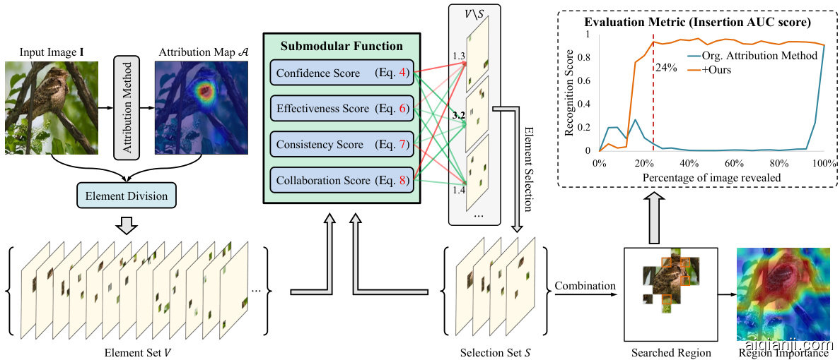
Figure 2: The framework of the proposed method.
图 2: 所提方法的框架。
4.1 SUB-REGION DIVISION
4.1 子区域划分
To obtain the interpret able region in an image, we partition the image $\mathbf{I}\in\mathbb{R}^{w\times h\times3}$ into $m$ subregions ${\bf\cal I}^{M}$ , where $M$ indicates a sub-region ${\bf\cal I}^{M}$ formed by masking part of image I. Traditional methods (Noroozi & Favaro, 2016; Redmon $&$ Farhadi, 2018) typically divide images into regular patch areas, neglecting the semantic information inherent in different regions. In contrast, our method employs a sub-region division strategy that is informed and guided by an a priori saliency map. In detail, we initially divide the image into $N\times N$ patch regions. Subsequently, an existing image attribution algorithm is applied to compute the saliency map $\boldsymbol{\mathcal{A}}\in\mathbb{R}^{w\times\dot{h}}$ for a corresponding class of I. Following this, we resize $\mathcal{A}$ to a $N\times N$ dimension, where its values denote the importance of each patch. Based on the determined importance of each patch, $d$ patches are sequentially allocated to each sub-region ${\bf\cal I}^{M}$ , while the remaining patch regions are masked with 0, where $d=N\times N/m$ . This process finally forms the element set $V={I{1}^{{M}},I{2}^{M},I{m}^{M}}$ , satisfying the condition $\begin{array}{r}{\mathbf{I}=\sum_{i=1}^{m}\mathbf{I}_{i}^{M}}\end{array}$ . The detailed calculation process is outlined in Algorithm 1.
为获取图像中的可解释区域,我们将图像 $\mathbf{I}\in\mathbb{R}^{w\times h\times3}$ 划分为 $m$ 个子区域 ${\bf\cal I}^{M}$ ,其中 $M$ 表示通过掩码图像I部分区域形成的子区域 ${\bf\cal I}^{M}$ 。传统方法 (Noroozi & Favaro, 2016; Redmon $&$ Farhadi, 2018) 通常将图像划分为规则块状区域,忽略了不同区域固有的语义信息。相比之下,我们的方法采用基于先验显著性图指导的子区域划分策略。具体而言,我们首先将图像划分为 $N\times N$ 个块状区域,随后应用现有图像归因算法计算对应类别I的显著性图 $\boldsymbol{\mathcal{A}}\in\mathbb{R}^{w\times\dot{h}}$ 。接着将 $\mathcal{A}$ 调整为 $N\times N$ 维度,其数值表示每个块的重要性。根据确定的各块重要性,依次为每个子区域 ${\bf\cal I}^{M}$ 分配 $d$ 个块(其中 $d=N\times N/m$ ),其余块区域用0掩码。最终形成满足条件 $\begin{array}{r}{\mathbf{I}=\sum_{i=1}^{m}\mathbf{I}{i}^{M}}\end{array}$ 的元素集 $V={I{1}^{{M}},I{2}^{M},I{m}^{M}}$ 。详细计算过程如算法1所示。
4.2 SUBMODULAR FUNCTION DESIGN
4.2 次模函数设计
Confidence Score We adopt a model trained by evidential deep learning (EDL) to quantify the uncertainty of a sample (Sensoy et al., 2018), which is developed to overcome the limitation of softmax-based networks in the open-set environment (Bao et al., 2021). We denote the network with prediction uncertainty by $\bar{F_{u}}(\cdot)$ . For $K$ -class classification, assume that the predicted class probability values follow a Dirichlet distribution. When given a sample $\mathbf{x}$ , the network is optimized by the following loss function:
置信度评分
我们采用基于证据深度学习(EDL)训练的模型来量化样本的不确定性(Sensoy等人, 2018),该模型旨在克服基于softmax的网络在开放集环境中的局限性(Bao等人, 2021)。我们用$\bar{F_{u}}(\cdot)$表示具有预测不确定性的网络。对于$K$类分类问题,假设预测的类别概率值服从狄利克雷分布。当给定样本$\mathbf{x}$时,网络通过以下损失函数进行优化:
$$
\mathcal{L}{E D L}=\sum_{k_{c}=1}^{K}\mathbf{y}{k_{c}}\left(\log S_{\mathrm{Dir}}-\log\left(\mathbf{e}{k_{c}}+1\right)\right),
$$
where $\mathbf{y}$ is the one-hot label of the sample $\mathbf{x}$ , and $\mathbf{e}\in\mathbb{R}^{K}$ is the output and the learned evidence of the network, denoted as $\mathbf{e}=\exp\left(F_{u}\left(\mathbf{x}\right)\right)$ . $\begin{array}{r}{S_{\mathrm{Dir}}=\sum_{k_{c}=1}^{K}\left(\mathbf{e}_{k_{c}}+1\right)}\end{array}$ is referred to as the Dirichlet strength. In the inference, the predictive uncertai nty can be calculated as $u=K/S_{\mathrm{Dir}}$ , where $u\in[0,1]$ . Thus, the confidence score of the sample $\mathbf{x}$ predicted by the network can be expressed as:
其中 $\mathbf{y}$ 是样本 $\mathbf{x}$ 的独热标签,$\mathbf{e}\in\mathbb{R}^{K}$ 是网络的输出和学习到的证据,表示为 $\mathbf{e}=\exp\left(F_{u}\left(\mathbf{x}\right)\right)$。$\begin{array}{r}{S_{\mathrm{Dir}}=\sum_{k_{c}=1}^{K}\left(\mathbf{e}_{k_{c}}+1\right)}\end{array}$ 被称为狄利克雷强度。在推理过程中,预测不确定性可计算为 $u=K/S_{\mathrm{Dir}}$,其中 $u\in[0,1]$。因此,网络预测样本 $\mathbf{x}$ 的置信度得分可表示为:
$$
s_{\mathrm{conf.}}\left(\mathbf{x}\right)=1-u=1-\frac{K}{\sum_{k_{c}=1}^{K}\left(\mathbf{e}_{k_{c}}+1\right)}.
$$
$$
s_{\mathrm{conf.}}\left(\mathbf{x}\right)=1-u=1-\frac{K}{\sum_{k_{c}=1}^{K}\left(\mathbf{e}_{k_{c}}+1\right)}.
$$
By incorporating the $S_{\mathrm{{conf}}}.$ , we can ensure that the selected regions align closely with the InDistribution (InD). This score acts as a reliable metric to distinguish regions from out-of-distribution, ensuring alignment with the InD.
通过引入 $S_{\mathrm{{conf}}}$ ,我们可以确保所选区域与同分布(InDistribution, InD)高度吻合。该分数作为区分同分布与异分布(out-of-distribution)区域的可靠指标,能有效保证与同分布的一致性。
Effectiveness Score We expect to maximize the response of valuable information with fewer regions since some image regions have the same semantic representation. Given an element $\alpha$ , and a
有效性得分
我们希望用更少的区域最大化有价值信息的响应,因为某些图像区域具有相同的语义表示。给定一个元素 $\alpha$ ,以及一个
sub-set $S$ , we measure the distance between the element $\alpha$ and all elements in the set, and calculate the smallest distance, as the effectiveness score of the judgment element $\alpha$ for the sub-set $S$ :
子集 $S$ 中,我们测量元素 $\alpha$ 与集合中所有元素之间的距离,并计算最小距离,作为判断元素 $\alpha$ 对于子集 $S$ 的有效性得分:
$$
s_{e}\left(\alpha\mid S\right)=\operatorname*{min}{s_{i}\in S}\mathrm{dist}\left(F\left(\alpha\right),F\left(s_{i}\right)\right),
$$
where $\mathrm{{dist}}(\cdot,\cdot)$ denotes the equation to calculate the distance between two elements. Traditional distance measurement methods (Wang et al., 2018; Deng et al., 2019) are tailored to maximize the decision margins between classes during model training, involving operations like feature scaling and increasing angle margins. In contrast, our method focuses solely on calculating the relative distance between features, for which we utilize the general cosine distance. $F(\cdot)$ denotes a pretrained feature extractor. To calculate the element effectiveness score of a set, we can compute the sum of the effectiveness scores for each element:
其中 $\mathrm{{dist}}(\cdot,\cdot)$ 表示计算两个元素间距离的公式。传统距离度量方法 (Wang et al., 2018; Deng et al., 2019) 专为在模型训练期间最大化类间决策边界而设计,涉及特征缩放和增大角度边界等操作。相比之下,我们的方法仅关注计算特征间的相对距离,为此我们采用通用的余弦距离。 $F(\cdot)$ 表示预训练的特征提取器。为计算集合中元素的效能得分,可对每个元素的效能得分进行求和:
$$
s_{\mathrm{eff.}}\left(S\right)=\sum_{s_{i}\in S}\operatorname{min}{s_{j}\in S,s_{i}\neq s_{j}}\operatorname{dist}\left(F\left(s_{i}\right),F\left(s_{j}\right)\right).
$$
By incorporating the $S_{\mathrm{eff.}}$ , we aim to limit the selection of regions with similar semantic representations, thereby increasing the diversity and improving the overall quality of region selection.
通过引入 $S_{\mathrm{eff.}}$ ,我们旨在限制具有相似语义表示的区域选择,从而增加多样性并提升区域选择的整体质量。
Consistency Score As the scores mentioned previously may be maximized by regions that aren’t target-dependent, we aim to make the representation of the identified image region consistent with the original semantics. Given a target semantic feature, $f_{s}$ , we make the semantic features of the searched image region close to the target semantic features. We introduce the consistency score:
一致性分数
由于前面提到的分数可能被非目标依赖区域最大化,我们的目标是使识别出的图像区域表示与原始语义保持一致。给定目标语义特征 $f_{s}$,我们使搜索到的图像区域的语义特征接近目标语义特征。我们引入一致性分数:
$$
s_{\mathrm{cons.}}\left(S,\mathbf{f}{s}\right)=\frac{F\left(\sum_{\mathbf{I}^{M}\in S}\mathbf{I}^{M}\right)\cdot\mathbf{\boldsymbol{f}}{s}}{\left|F\left(\sum_{\mathbf{I}^{M}\in S}\mathbf{I}^{M}\right)\right|\left|\mathbf{\boldsymbol{f}}_{s}\right|},
$$
where $F(\cdot)$ denotes a pre-trained feature extractor. The target semantic feature $f_{s}$ , can either adopt the features computed from the original image using the pre-trained feature extractor, expressed as ${f}{s}=F\left(\mathbf{I}\right)$ , or directly implement the fully connected layer of the classifier for a specified class. By incorporating the $s_{\mathrm{cons.}}$ ., our method targets regions that reinforce the desired semantic response. This approach ensures a precise selection that aligns closely with our specific semantic goals.
其中 $F(\cdot)$ 表示预训练的特征提取器。目标语义特征 $f_{s}$ 既可采用预训练特征提取器从原始图像计算得到的特征(表示为 ${f}{s}=F\left(\mathbf{I}\right)$,也可直接使用指定分类器的全连接层。通过引入 $s_{\mathrm{cons.}}$,我们的方法聚焦于强化目标语义响应的区域。该策略确保精准选择符合特定语义目标的区域。
where $F(\cdot)$ denotes a pre-trained feature extractor, $f_{s}$ is the target semantic feature. By introducing the collaboration score, we can judge the collective effect of the element. By incorporating the $s_{\mathrm{colla.}}$ , our method pinpoints regions whose exclusion markedly affects the model’s predictive confidence. This effect underscores the pivotal role of these regions, indicative of a significant collective impact. Such a metric is particularly valuable in the initial stages of the search, highlighting regions essential for sustaining the model’s accuracy and reliability.
其中 $F(\cdot)$ 表示预训练的特征提取器,$f_{s}$ 是目标语义特征。通过引入协作分数 (collaboration score) ,我们可以评估元素的集体效应。结合 $s_{\mathrm{colla.}}$ 后,我们的方法能精确定位那些被排除时会显著影响模型预测置信度的区域。这种效应凸显了这些区域的关键作用,表明它们具有重要的集体影响力。该指标在搜索初始阶段尤为重要,能突出对维持模型准确性和可靠性至关重要的区域。
Submodular Function We construct our objective function for selecting elements through a combination of the above scores, ${\mathcal{F}}(S)$ , as follows:
子模函数
我们通过结合上述分数构建用于选择元素的目标函数 ${\mathcal{F}}(S)$,具体如下:
$$
\mathcal{F}(S)=\lambda_{1}s_{\mathrm{conf.}}\left(\sum_{\mathbf{I}^{M}\in S}\mathbf{I}^{M}\right)+\lambda_{2}s_{\mathrm{eff.}}\left(S\right)+\lambda_{3}s_{\mathrm{cons.}}\left(S,\pmb{f}{s}\right)+\lambda_{4}s_{\mathrm{colla.}}\left(S,\mathbf{I},\pmb{f}_{s}\right),
$$
where $\lambda_{1},\lambda_{2},\lambda_{3}$ , and $\lambda_{4}$ represent the weighting factors used to balance each score. To simplify parameter adjustment, all weighting coefficients are set to 1 by default.
其中 $\lambda_{1}$、$\lambda_{2}$、$\lambda_{3}$ 和 $\lambda_{4}$ 表示用于平衡各得分的权重因子。为简化参数调整,默认将所有权重系数设为1。
Lemma 1. Consider two sub-sets $S_{a}$ and $S_{b}$ in set $V$ , where $S_{a}\subseteq S_{b}\subseteq V$ . Given an element $\alpha$ , where $\alpha\in V\backslash S_{b}$ . Assuming that $\alpha$ is contributing to model interpretation, then, the function ${\mathcal{F}}(\cdot)$ in Eq. 9 is a submodular function and satisfies Eq. 1.
引理 1. 考虑集合 $V$ 中的两个子集 $S_{a}$ 和 $S_{b}$ ,其中 $S_{a}\subseteq S_{b}\subseteq V$ 。给定元素 $\alpha$ ,且 $\alpha\in V\backslash S_{b}$ 。若 $\alpha$ 对模型解释有贡献,则式 9 中的函数 ${\mathcal{F}}(\cdot)$ 是次模函数并满足式 1。
Proof. Please see Appendix B.1 for the proof.
证明。具体证明过程请参见附录 B.1。
Lemma 2. Consider a subset $S$ , given an element α, assuming that α is contributing to model interpretation. The function $\mathcal{F}(\cdot)$ of Eq. 9 is monotonically non-decreasing.
引理 2. 考虑一个子集 $S$,给定一个元素 α,假设 α 对模型解释有贡献。则公式 9 中的函数 $\mathcal{F}(\cdot)$ 是单调非减的。
Proof. Please see Appendix B.2 for the proof.
证明。具体证明过程请参见附录 B.2。
4.3 GREEDY SEARCH ALGORITHM
4.3 贪心搜索算法
Algorithm 1: A greedy search based algorithm for interpret able region discovery
算法 1: 基于贪心搜索的可解释区域发现算法
Given a set $V={I{1}^{M},I{2}^{M},I_{m}^{M}}$ , we can follow Eq. 2 to search the interpret able region by selecting elements that maximize the value of the submodular function . The above problem can be effectively addressed by implementing a greedy search algorithm. Referring to related works (Mirza sole iman et al., 2015; Wei et al., 2015), we use Algorithm 1 to optimize the value of the submodular function. Based on Lemma 1 and Lemma 2 we have proved that the function ${\mathcal{F}}(\cdot)$ is a submodular function. According to the theory of Nemhauser et al. (1978), we have:
给定集合 $V={I_{1}^{M},I_{2}^{M},I_{m}^{M}}$,我们可以根据公式2通过选择使子模函数值最大化的元素来搜索可解释区域。上述问题可以通过实现贪心搜索算法有效解决。参考相关研究 (Mirza sole iman et al., 2015; Wei et al., 2015),我们使用算法1来优化子模函数的值。基于引理1和引理2,我们已证明函数 ${\mathcal{F}}(\cdot)$ 是一个子模函数。根据Nemhauser等人 (1978) 的理论,我们有:
Theorem 1 ((Nemhauser et al., 1978)). Let $S$ denotes the solution obtained by the greedy search approach, and $S^{*}$ denotes the optimal solution. If $\mathcal{F}(\cdot)$ is a submodular function, then the solution $S$ has the following approximation guarantee:
定理1 (Nemhauser et al., 1978). 设$S$表示贪心搜索算法得到的解,$S^{*}$表示最优解。若$\mathcal{F}(\cdot)$是次模函数(submodular function),则解$S$具有以下近似保证:
$$
\mathcal{F}(S)\geq\left(1-\frac{1}{\mathrm{e}}\right)\mathcal{F}(S^{\ast}),
$$
$$
\mathcal{F}(S)\geq\left(1-\frac{1}{\mathrm{e}}\right)\mathcal{F}(S^{\ast}),
$$
where e is the base of natural logarithm.
其中 e 是自然对数的底数。
5 EXPERIMENTS
5 实验
5.1 EXPERIMENTAL SETUP
5.1 实验设置
Datasets We evaluate the proposed method on two face datasets Celeb-A (Liu et al., 2015) and VGG-Face2 (Cao et al., 2018), and a fine-grained dataset CUB-200-2011 (Welinder et al., 2010). Celeb-A dataset includes 10, 177 IDs, we randomly select 2, 000 identities from Celeb-A’s validation set, and one test face image for each identity is used to evaluate our method; the VGG-Face2 dataset includes 8, 631 IDs, we randomly select 2, 000 identities from VGG-Face2’s validation set, and one test face image for each identity is used to evaluate our method; CUB-200-2011 dataset includes 200 bird species, we select 3 samples for each class that is correctly predicted by the model from the CUB-200-2011 validation set for 200 classes, a total of 600 images are used to evaluate the image attribution effect. Additionally, 2 incorrectly predicted samples from each class are selected, totaling 400 images, to evaluate our method for identifying the cause of model prediction errors.
数据集
我们在两个人脸数据集Celeb-A (Liu et al., 2015) 和VGG-Face2 (Cao et al., 2018) 以及一个细粒度数据集CUB-200-2011 (Welinder et al., 2010) 上评估所提出的方法。Celeb-A数据集包含10,177个ID,我们从中随机选取2,000个身份,并使用每个身份的一张测试人脸图像来评估我们的方法;VGG-Face2数据集包含8,631个ID,我们从中随机选取2,000个身份,并使用每个身份的一张测试人脸图像来评估我们的方法;CUB-200-2011数据集包含200种鸟类,我们从CUB-200-2011验证集中为每个类别选取3个被模型正确预测的样本(共200类),总计600张图像用于评估图像归因效果。此外,从每个类别中选取2个预测错误的样本,总计400张图像,用于评估我们识别模型预测错误原因的方法。
Table 1: Deletion and Insertion AUC scores on the Celeb-A, VGG-Face2, and CUB-200-2011 validation sets.
表 1: Celeb-A、VGG-Face2 和 CUB-200-2011 验证集上的删除与插入 AUC 分数。
| 方法 | Celeb-A | Celeb-A | VGGFace2 | VGGFace2 | CUB-200-2011 | CUB-200-2011 |
|---|---|---|---|---|---|---|
| 删除(↓) | 插入(↑) | 删除(↓) | 插入(↑) | 删除(↓) | 插入(↑) | |
| Saliency (Simonyan et al., 2014) | 0.1453 | 0.4632 | 0.1907 | 0.5612 | 0.0682 | 0.6585 |
| Saliency (w/ours) | 0.1254 | 0.5465 | 0.1589 | 0.6287 | 0.0675 | 0.6927 |
| Grad-CAM (Selvaraju et al., 2020) | 0.2865 | 0.3721 | 0.3103 | 0.4733 | 0.0810 | 0.7224 |
| Grad-CAM (w/ours) | 0.1549 | 0.4927 | 0.1982 | 0.5867 | 0.0726 | 0.7231 |
| LIME (Ribeiro et al., 2016) | 0.1484 | 0.5246 | 0.2034 | 0.6185 | 0.1070 | 0.6812 |
| LIME (w/ours) | 0.1366 | 0.5496 | 0.1653 | 0.6314 | 0.0941 | 0.6994 |
| Kernel Shap (Lundberg & Lee, 2017) | 0.1409 | 0.5246 | 0.2119 | 0.6132 | 0.1016 | 0.6763 |
| KernelShap (w/ours) | 0.1352 | 0.5504 | 0.1669 | 0.6314 | 0.0951 | 0.6920 |
| RISE (Petsiuk et al., 2018) | 0.1444 | 0.5703 | 0.1375 | 0.6530 | 0.0665 | 0.7193 |
| RISE (w/ours) | 0.1264 | 0.5719 | 0.1346 | 0.6548 | 0.0630 | 0.7245 |
| HSIC-Attribution (Novello et al., 2022) | 0.1151 | 0.5692 | 0.1317 | 0.6694 | 0.0647 | 0.6843 |
| HSIC-Attribution (w/ours) | 0.1054 | 0.5752 | 0.1304 | 0.6705 | 0.0613 | 0.7262 |
Evaluation Metric We use Deletion and Insertion AUC scores (Petsiuk et al., 2018) to evaluate the faithfulness of our method in explaining model predictions. To evaluate the ability of our method to search for causes of model prediction errors, we use the model’s highest confidence in correct class predictions over different search ranges as the evaluation metric.
评估指标
我们采用Deletion和Insertion AUC分数 (Petsiuk et al., 2018) 来评估本方法在解释模型预测时的忠实度。为评估本方法在搜索模型预测错误原因时的能力,我们使用模型在不同搜索范围内对正确类别预测的最高置信度作为评估指标。
Baselines We select the following popular attribution algorithm for calculating the prior saliency map in Sec. 4.1, and also for comparison methods, including the white-box-based methods: Saliency (Simonyan et al., 2014), Grad-CAM (Selvaraju et al., 2020), Grad $\mathrm{CAM++}$ (Chat to pad hay et al., 2018), Score-CAM (Wang et al., 2020), and the black-box-based methods: LIME (Ribeiro et al., 2016), Kernel Shap (Lundberg & Lee, 2017), RISE (Petsiuk et al., 2018) and HSICAttribution (Novello et al., 2022).
基线方法
我们选择了以下流行的归因算法来计算第4.1节中的先验显著图,并作为对比方法,包括基于白盒的方法:Saliency (Simonyan et al., 2014)、Grad-CAM (Selvaraju et al., 2020)、Grad $\mathrm{CAM++}$ (Chat to pad hay et al., 2018)、Score-CAM (Wang et al., 2020),以及基于黑盒的方法:LIME (Ribeiro et al., 2016)、Kernel Shap (Lundberg & Lee, 2017)、RISE (Petsiuk et al., 2018) 和 HSICAttribution (Novello et al., 2022)。
Implementation Details Please see Appendix C for details.
实现细节
详情请参阅附录 C。
5.2 FAITHFULNESS ANALYSIS
5.2 忠实度分析
To highlight the superiority of our method, we evaluate its faithfulness, which gauges the consistency of the generated explanations with the deep model’s decision-making process (Li et al., 2021a). We use Deletion and Insertion AUC scores to form the evaluation metric, which measures the decrease (or increase) in class probability as important pixels (given by the saliency map) are gradually removed (or increased) from the image. Since our method is based on greedy search, we can determine the importance of the divided regions according to the order in which they are searched. We can evaluate the faithfulness of the method by comparing the Deletion or Insertion scores under different image perturbation scales (i.e. different $k$ sizes) with other attribution methods. We set the search subset size $k$ to be the same as the set size $m$ , and adjust the size of the divided regions according to the order of the returned elements. The image is perturbed to calculate the value of Deletion or Insertion of our method.
为突显本方法的优越性,我们评估了其忠实度(faithfulness),该指标衡量生成解释与深度模型决策过程的一致性(Li et al., 2021a)。采用删除(Deletion)和插入(Insertion) AUC分数构建评估指标,该指标通过逐步移除(或增加)图像中显著图给出的重要像素时,类别概率的下降(或上升)程度进行度量。由于本方法基于贪心搜索(greedy search),可根据区域被搜索的先后顺序确定划分区域的重要性。通过比较不同图像扰动尺度(即不同$k$值)下的删除或插入分数与其他归因方法的差异,即可评估方法的忠实度。我们将搜索子集大小$k$设为与集合大小$m$相同,并根据返回元素的顺序调整划分区域尺寸,通过图像扰动计算本方法的删除或插入值。
Table 1 shows the results on the Celeb-A, VGG-Face2, and CUB-200-2011 validation sets. We find that no matter which attribution method’s saliency map is used as the baseline, our method can improve its Deletion and Insertion scores. The performance of our approach is also directly influenced by the sophistication of the underlying attribution algorithm, with more advanced algorithms leading to superior results. The state-of-the-art method, HSIC-Attribution (Novello et al., 2022), shows improvements when combined with our method. On the Celeb-A dataset, our method reduces its Deletion score by $8.4%$ and improves its Insertion score by $1.1%$ . Similarly, on the CUB-200- 2011 dataset, our method enhances the HSIC-Attribution method by reducing its Deletion score by $5.3%$ and improving its Insertion score by $6.1%$ . On the VGG-Face2 dataset, our method enhances the HSIC-Attribution method by reducing its Deletion score by $1.0%$ and improving its Insertion score by $0.2%$ , this slight improvement may be caused by the large number of noisy images in the VGG-Face2 dataset. It is precise because we reformulate the image attribution problem into a subset selection problem that we can alleviate the insufficient fine-graininess of the attribution region, thus improving the faithfulness of existing attribution algorithms. Our method exhibits significant improvements across a spectrum of vision tasks and attribution algorithms, thereby highlighting its extensive general iz ability. Please see Appendix $\mathrm{H}$ for visualization s of our method on these datasets.
表 1: 展示了在Celeb-A、VGG-Face2和CUB-200-2011验证集上的结果。我们发现,无论使用哪种归因方法的显著性图作为基线,我们的方法都能提升其Deletion和Insertion分数。我们方法的性能也直接受到底层归因算法复杂程度的影响,更先进的算法会带来更优异的结果。当前最先进的方法HSIC-Attribution (Novello et al., 2022) 在与我们的方法结合时也显示出改进。在Celeb-A数据集上,我们的方法将其Deletion分数降低了$8.4%$,并将Insertion分数提高了$1.1%$。同样,在CUB-200-2011数据集上,我们的方法通过将HSIC-Attribution方法的Deletion分数降低$5.3%$并将Insertion分数提高$6.1%$来增强其性能。在VGG-Face2数据集上,我们的方法通过将HSIC-Attribution方法的Deletion分数降低$1.0%$并将Insertion分数提高$0.2%$来增强其性能,这种微小的改进可能是由于VGG-Face2数据集中存在大量噪声图像所致。正是因为我们重新将图像归因问题表述为一个子集选择问题,我们才能缓解归因区域细粒度不足的问题,从而提高现有归因算法的忠实度。我们的方法在一系列视觉任务和归因算法中均表现出显著改进,从而突显了其广泛的泛化能力。请参阅附录$\mathrm{H}$以查看我们的方法在这些数据集上的可视化结果。
Table 2: Evaluation of discovering the cause of incorrect predictions.
表 2: 错误预测原因发现的评估
| 方法 | (0-25%) | (0-50%) | (0-75%) | (0-100%) | 插入(↑) |
|---|---|---|---|---|---|
| Grad-CAM++ (Chattopadhay et al., 2018) | 0.1988 | 0.2447 | 0.2544 | 0.2647 | 0.1094 |
| Grad-CAM++(w/ours) | 0.2424 | 0.3575 | 0.3934 | 0.4193 | 0.1672 |
| Score-CAM (Wang et al., 2020) | 0.1896 | 0.2323 | 0.2449 | 0.2510 | 0.1073 |
| Score-CAM(w/ours) | 0.2491 | 0.3395 | 0.3796 | 0.4082 | 0.1622 |
| HSIC-Attribution (Novello et al., 2022) | 0.1709 | 0.2091 | 0.2250 | 0.2493 | 0.1446 |
| HSIC-Attribution(w/ours) | 0.2430 | 0.3519 | 0.3984 | 0.4513 | 0.1772 |
| Patch10x10 | 0.2020 | 0.4065 | 0.4908 | 0.5237 | 0.1519 |

Figure 3: Visualization of the method for discovering what causes model prediction errors. The Insertion curve shows the correlation between the searched region and ground truth class prediction confidence. The highlighted region matches the searched region indicated by the red line in the curve, and the dark region is the error cause identified by the method.
图 3: 模型预测错误原因发现方法可视化。插入曲线 (Insertion curve) 显示搜索区域与真实类别预测置信度的相关性。高亮区域对应曲线中红线标识的搜索区域,深色区域为该方法识别出的错误原因。
5.3 DISCOVER THE CAUSES OF INCORRECT PREDICTIONS
5.3 探索错误预测的原因
In this section, we analyze the images that are mis classified in the CUB-200-2011 validation set and try to discover the causes for their mis classification. We use Grad ${\cal{C}}{\mathrm{AM}}{+}{+}$ , Score-CAM, and HSIC-Attribution as baseline. We specify its ground truth class and use our attribution algorithm to discover regions where the model’s response improves on that class as much as possible. We evaluate the performance of each method using the highest confidence score found within different search ranges. For instance, we determine the highest category prediction confidence that the algorithm can discover by searching up to $25%$ of the image region (i.e., set $k=0.25m$ ). We also introduce the Insertion AUC score as an evaluation metric.
在本节中,我们分析了CUB-200-2011验证集中被错误分类的图像,并试图找出其误分类的原因。我们使用Grad ${\cal{C}}{\mathrm{AM}}{+}{+}$、Score-CAM和HSIC-Attribution作为基线方法。指定其真实类别后,利用我们的归因算法发现模型在该类别上响应尽可能提升的区域。通过在不同搜索范围内找到的最高置信度分数来评估每种方法的性能。例如,通过搜索至多$25%$的图像区域(即设$k=0.25m$)来确定算法能发现的最高类别预测置信度。我们还引入了插入AUC分数作为评估指标。
Table 2 shows the results for samples that were mis classified in the CUB-200-2011 validation set, we find that our method achieves significant improvements. The average highest confidence score searched by our method in any search interval is higher than the baseline. In the global search interval $(0\small{-}100%)$ , the average highest confidence level searched by our method is improved by $58.4%$ on Grad $\mathrm{CAM++}$ , $62.6%$ on Score-CAM, and $81.0%$ on HSIC-Attribution. Its Insertion score has also been significantly improved, increasing by $52.8%$ on Grad ${\cal{C}}{\mathrm{AM}}{+}{+}$ , $51.2%$ on ScoreCAM, and $18.4%$ on HSIC-Attribution. In another scenario, our method does not rely on the saliency map of the attribution algorithm as a priori. Instead, it divides the image into $N\times N$ patches, where each element in the set contains only one patch. In this case, our method achieves a higher average highest confidence score, in the global search interval $(0\small{-}100%)$ ), our method (divide the image into $10\times10$ patches) is $97.8%$ better than Grad $C_{\mathrm{{AM++}}}$ , $108.6%$ better than Score-CAM, and $110.1%$ better than HSIC-Attribution. Fig. 3 shows some visualization results, we compare our method with the SOTA method HSIC-Attribution. The Insertion curve represents the relationship between the region searched by the methods and the ground truth class prediction confidence. We find that our method can search for regions with higher confidence scores predicted by the model than the HSICAttribution method with a small percentage of the searched image region. The highlighted region shown in the figure can be considered as the cause of the correct prediction of the model, while the dark region is the cause of the incorrect prediction of the model. This also demonstrates that our method can achieve higher interpret ability with fewer fine-grained regions. For further experiments and analysis of this method across various network backbones, please refer to Appendix D.
表 2 展示了在 CUB-200-2011 验证集中被错误分类的样本结果,我们发现我们的方法取得了显著改进。我们的方法在任何搜索区间内搜索到的平均最高置信度分数均高于基线。在全局搜索区间 $(0{-}100%)$ 内,我们的方法搜索到的平均最高置信度水平在 Grad $\mathrm{CAM++}$ 上提高了 $58.4%$,在 Score-CAM 上提高了 $62.6%$,在 HSIC-Attribution 上提高了 $81.0%$。其插入分数也有显著提升,在 Grad ${\cal{C}}{\mathrm{AM}}{+}{+}$ 上增加了 $52.8%$,在 ScoreCAM 上增加了 $51.2%$,在 HSIC-Attribution 上增加了 $18.4%$。在另一种场景下,我们的方法不依赖归因算法的显著性图作为先验,而是将图像划分为 $N\times N$ 的块,其中集合中的每个元素仅包含一个块。在这种情况下,我们的方法实现了更高的平均最高置信度分数,在全局搜索区间 $(0{-}100%)$ 内,我们的方法(将图像划分为 $10\times10$ 的块)比 Grad $C_{\mathrm{{AM++}}}$ 高出 $97.8%$,比 Score-CAM 高出 $108.6%$,比 HSIC-Attribution 高出 $110.1%$。图 3 展示了一些可视化结果,我们将我们的方法与 SOTA 方法 HSIC-Attribution 进行了比较。插入曲线表示方法搜索到的区域与真实类别预测置信度之间的关系。我们发现,与 HSIC-Attribution 方法相比,我们的方法能够以较小的搜索图像区域比例搜索到模型预测的更高置信度分数的区域。图中高亮显示的区域可视为模型正确预测的原因,而暗色区域则是模型错误预测的原因。这也表明我们的方法能够以更少的细粒度区域实现更高的可解释性。有关该方法在各种网络骨干上的进一步实验和分析,请参阅附录 D。
Table 3: Ablation study on components of different score functions of submodular function on the Celeb-A, and CUB-200-2011 validation sets.
表 3: 子模函数不同得分函数组件在Celeb-A和CUB-200-2011验证集上的消融研究。
| SubmodularFunction | Celeb-A | CUB-200-2011 |
|---|---|---|
| Conf.Score (Equation 4) | Eff. Score (Equation 6) | Cons.Score (Equation 7) |
| × | ||
| × | × | |
| × | × | |
| × | ||
| √ | ||
| × | √ | |
| √ | ||
| √ | × | |
| √ | √ | × |
| √ | √ | |
| √ |
Table 4: Impact on whether to use a priori attribution map.
表 4: 是否使用先验归因图的影响
| 方法 | 划分集大小 m | Celeb-A | CUB-200-2011 | ||
|---|---|---|---|---|---|
| 删除 (↓) | 插入 (↑) | 删除 (↓) | 插入 (↑) | ||
| Patch7x7 | 49 | 0.1493 | 0.5642 | 0.1061 | 0.6903 |
| Patch10x10 | 100 | 0.1365 | 0.5459 | 0.1024 | 0.6159 |
| Patch14x14 | 196 | 0.1284 | 0.5562 | 0.0853 | 0.5805 |
| +HSIC-Attribution | 25 | 0.1054 | 0.5752 | 0.0613 | 0.7262 |
5.4 ABLATION STUDY
5.4 消融实验
Components of Submodular Function We analyze the impact of various submodular functionbased score functions on the results for both the Celeb-A and CUB-200-2011 datasets, the saliency map generated by the HSIC-Attribution method is used as a prior. As shown in Table 3, we observed that using a single score function within the submodular function limits attribution faithfulness. When these score functions are combined in pairs, the faithfulness of our method will be further improved. We demonstrate that removing any of the four score functions leads to deteriorated Deletion and Insertion scores, confirming the validity of these score functions. We find that the effectiveness score is key for the Celeb-A dataset, while the collaboration score is more important for the CUB-200-2011 dataset.
子模函数组件分析
我们分析了基于不同子模函数的评分函数对Celeb-A和CUB-200-2011数据集结果的影响,其中HSIC-Attribution方法生成的显著图作为先验。如表3所示,我们观察到在子模函数中使用单一评分函数会限制归因的忠实性。当这些评分函数两两组合时,我们方法的忠实性会进一步提升。实验证明,移除四个评分函数中的任意一个都会导致Deletion和Insertion分数下降,验证了这些评分函数的有效性。我们发现有效性评分对Celeb-A数据集起关键作用,而协作评分对CUB-200-2011数据集更为重要。
Whether to Use a Priori Attribution Map Our method uses existing attribution algorithms as priors when dividing the image into sub-regions. Table 4 shows the results, we directly divide the image into $N\times N$ patches without using a priori attribution map. Each element in the set only retains the pixel value of one patch area, and other areas are filled with values 0. We can observe that, whether on the Celeb-A dataset or the CUB-200-2011 dataset, the more patches are divided, the Deletion AUC score increases, and the fewer patches are divided, the Insertion AUC score increases. However, no matter how the number of patches is changed, we find that introducing a prior saliency map generated by the HSIC attribution method works best, in terms of Insertion or Deletion scores. Therefore, we believe that introducing a prior saliency map to assist in dividing image areas is effective and can improve the computational efficiency of the algorithm.
是否使用先验归因图
我们的方法在将图像划分为子区域时,会使用现有归因算法作为先验。表4展示了结果:我们直接将图像划分为$N\times N$个补丁而不使用先验归因图。集合中的每个元素仅保留一个补丁区域的像素值,其他区域用0填充。可以观察到,无论在Celeb-A数据集还是CUB-200-2011数据集上,划分的补丁越多,Deletion AUC分数越高;划分的补丁越少,Insertion AUC分数越高。但无论补丁数量如何变化,我们发现引入HSIC归因方法生成的先验显著图效果最佳(无论是Insertion还是Deletion分数)。因此,我们认为引入先验显著图辅助划分图像区域是有效的,并能提升算法的计算效率。
6 CONCLUSION
6 结论
In this paper, we propose a new method that reformulates the attribution problem as a submodular subset selection problem. To address the lack of attention to local regions, we construct a novel submodular function to discover more accurate fine-grained interpretation regions. Specifically, four different constraints implemented on sub-regions are formulated together to evaluate the significance of various subsets, i.e., confidence, effectiveness, consistency, and collaboration scores. The proposed method has outperformed state-of-the-art methods on two face datasets (Celeb-A and VGG-Face2) and a fine-grained dataset (CUB-200-2011). Experimental results show that the proposed method can improve the Deletion and Insertion scores for the correctly predicted samples. While for incorrectly predicted samples, our method excels in identifying the reasons behind the model’s decision-making errors.
本文提出了一种新方法,将归因问题重新表述为子模子集选择问题。针对局部区域关注不足的问题,我们构建了一个新颖的子模函数来发现更准确的细粒度解释区域。具体而言,通过整合子区域的四个约束条件(置信度、有效性、一致性和协作性评分)来评估不同子集的重要性。该方法在两个人脸数据集(Celeb-A和VGG-Face2)和一个细粒度数据集(CUB-200-2011)上超越了现有最优方法。实验结果表明,所提方法能提升正确预测样本的Deletion和Insertion分数,对于错误预测样本则能有效识别模型决策失误的原因。
ACKNOWLEDGMENTS
致谢
This work was supported in part by the National Key R&D Program of China (Grant No. 2022 ZD 0118102), in part by the National Natural Science Foundation of China (No. 62372448, 62025604, 62306308), and part by Beijing Natural Science Foundation (No. L212004).
本研究部分由国家重点研发计划(No. 2022ZD0118102)、国家自然科学基金(No. 62372448, 62025604, 62306308)和北京市自然科学基金(No. L212004)资助。
A NOTATIONS
符号说明
The notations used throughout this article are summarized in Table 5.
本文使用的符号标记总结如表5所示。
Table 5: Some important notations used in this paper.
表 5: 本文使用的一些重要符号。
| 符号 | 描述 |
|---|---|
| I | 输入图像 |
| IM | I 划分的子区域 |
| V | 划分的子区域有限集合 |
| S | V 的子集 |
| α | 来自 V\ S 的元素 |
| k | S 的大小 |
| F() | 将集合映射到值的函数 |
| A | 通过归因算法计算的显著性图 |
| N× N | I 划分的区块数量 |
| m | 图像 I 划分的子区域数量 |
| d | IM 中的区块数量 |
| X | 输入样本 |
| y | one-hot 标签 |
| u | 预测不确定性(范围从 0 到 1) |
| Fu() | 用于计算 x 的 u 的深度证据网络 |
| F() | 传统网络编码器 |
| K | 类别数量 |
| dist(,) | 计算两个特征向量之间距离的函数 |
| fs | 目标语义特征向量 |
B THEORY PROOF
B 理论证明
B.1 PROOF OF LEMMA 1
B.1 引理1的证明
Proof. Consider two sub-sets $S_{a}$ and $S_{b}$ in set $V$ , where $S_{a}\subseteq S_{b}\subseteq V$ . Given an element $\alpha$ , where $\alpha=V\backslash S_{b}$ . The necessary and sufficient conditions for the function $\mathcal{F}(\cdot)$ to satisfy the submodular property are:
证明。考虑集合 $V$ 中的两个子集 $S_{a}$ 和 $S_{b}$,其中 $S_{a}\subseteq S_{b}\subseteq V$。给定元素 $\alpha$,其中 $\alpha=V\backslash S_{b}$。函数 $\mathcal{F}(\cdot)$ 满足子模性质的充要条件是:
$$
(S_{a}{})-F(S_{a})F(S_{b}{})-F(S_{b}).
$$
For Eq. 4, assuming that the individual element $\alpha$ of the collection division is relatively small, according to the Taylor decomposition (Montavon et al., 2017), we can locally approximate $\dot{F}{u}(S_{a}+$ $\alpha)=F_{u}(\boldsymbol{\bar{S}}\alpha)+\nabla\dot{F}{u}(\boldsymbol{S}_{a})\cdot\boldsymbol{\alpha}$ . Thus:
对于式4,假设集合划分的单个元素$\alpha$相对较小,根据泰勒分解 (Montavon et al., 2017),我们可以局部近似$\dot{F}{u}(S_{a}+$$\alpha)=F_{u}(\boldsymbol{\bar{S}}\alpha)+\nabla\dot{F}{u}(\boldsymbol{S}_{a})\cdot\boldsymbol{\alpha}$。因此:
$$
\begin{array}{c}{{s_{\mathrm{conf.}}\left(S_{a}+\alpha\right)-s_{\mathrm{conf.}}\left(S_{a}\right)=\displaystyle\frac{K}{\exp\left(F_{u}\left(S_{a}\right)\right)+K}-\displaystyle\frac{K}{\exp\left(F_{u}\left(S_{a}+\alpha\right)\right)+K}}}\ {{=\displaystyle\frac{K}{\exp\left(F_{u}\left(S_{a}\right)\right)+K}-\displaystyle\frac{K}{\exp\left(F_{u}\left(S_{a}\right)\right)\exp\left(\nabla F_{u}\left(S_{a}\right)\cdot\alpha\right)+K},}}\end{array}
$$
$$
\begin{array}{c}{{s_{\mathrm{conf.}}\left(S_{a}+\alpha\right)-s_{\mathrm{conf.}}\left(S_{a}\right)=\displaystyle\frac{K}{\exp\left(F_{u}\left(S_{a}\right)\right)+K}-\displaystyle\frac{K}{\exp\left(F_{u}\left(S_{a}+\alpha\right)\right)+K}}}\ {{=\displaystyle\frac{K}{\exp\left(F_{u}\left(S_{a}\right)\right)+K}-\displaystyle\frac{K}{\exp\left(F_{u}\left(S_{a}\right)\right)\exp\left(\nabla F_{u}\left(S_{a}\right)\cdot\alpha\right)+K},}}\end{array}
$$
since $S_{a}\cap\alpha=\emptyset,$ $S_{a}$ and $\alpha$ do not overlap in the image space, and $\alpha$ is small. Therefore, we can regard $\nabla F_{u}(S_{a})\cdot\alpha\simeq0$ . Follow up:
由于 $S_{a}\cap\alpha=\emptyset$ ,$S_{a}$ 和 $\alpha$ 在图像空间中不重叠,且 $\alpha$ 较小。因此,我们可以认为 $\nabla F_{u}(S_{a})\cdot\alpha\simeq0$ 。后续:
$$
s_{\mathrm{conf.}}\left(S_{a}+\alpha\right)-s_{\mathrm{conf.}}\left(S_{a}\right)\simeq\frac{K}{\exp\left(F_{u}\left(S_{a}\right)\right)+K}-\frac{K}{\exp\left(F_{u}\left(S_{a}\right)\right)\exp\left(\mathbf{0}\right)+K}
$$
$$
s_{\mathrm{conf.}}\left(S_{a}+\alpha\right)-s_{\mathrm{conf.}}\left(S_{a}\right)\simeq\frac{K}{\exp\left(F_{u}\left(S_{a}\right)\right)+K}-\frac{K}{\exp\left(F_{u}\left(S_{a}\right)\right)\exp\left(\mathbf{0}\right)+K}
$$
and in the same way, $s_{\mathrm{conf.}}\left(S_{b}+\alpha\right)-s_{\mathrm{conf.}}\left(S_{b}\right)\simeq0_{+},$ . We have:
同样地,$s_{\mathrm{conf.}}\left(S_{b}+\alpha\right)-s_{\mathrm{conf.}}\left(S_{b}\right)\simeq0_{+},$。我们有:
$$
s_{\mathrm{conf.}}\left(S_{a}+\alpha\right)-s_{\mathrm{conf.}}\left(S_{a}\right)-\left(s_{\mathrm{conf.}}\left(S_{b}+\alpha\right)-s_{\mathrm{conf.}}\left(S_{b}\right)\right)\approx0.
$$
$$
s_{\mathrm{conf.}}\left(S_{a}+\alpha\right)-s_{\mathrm{conf.}}\left(S_{a}\right)-\left(s_{\mathrm{conf.}}\left(S_{b}+\alpha\right)-s_{\mathrm{conf.}}\left(S_{b}\right)\right)\approx0.
$$
where $\varepsilon_{a}$ is a constant, which is the sum of the minimum distance reductions of the elements in the original $S_{a}$ after $\alpha$ is added. Then, we have:
其中 $\varepsilon_{a}$ 是一个常数,表示原始 $S_{a}$ 中的元素在加入 $\alpha$ 后的最小距离减少量之和。于是我们得到:
$$
s_{eff.}(S_{a}{})-s_{eff.}(S_{a})=min{s_{i} S_{a}}dist(F),F(s_{i}))-_{a},
$$
and in the same way,
同样地,
$$
s_{eff.}(S_{b}{})-s_{eff.}(S_{b})={min}{s_{i} S_{b}}dist(F,F(s_{i}))-_{b},
$$
since $S_{a}\subseteq S_{b}$ , the minimum distance between alpha and elements in $S_{b}\setminus S_{a}$ may be smaller than the minimum distance between alpha and elements in $S_{a}$ , thus,
由于 $S_{a}\subseteq S_{b}$,alpha 与 $S_{b}\setminus S_{a}$ 中元素的最小距离可能小于 alpha 与 $S_{a}$ 中元素的最小距离,因此,
$$
\operatorname{min}{s_{i}\in S_{a}}\operatorname{dist}\left(F\left(\alpha\right),F\left(s_{i}\right)\right)\geq\operatorname{min}{s_{i}\in S_{b}}\operatorname{dist}\left(F\left(\alpha\right),F\left(s_{i}\right)\right),
$$
since there are more elements in $S_{b}$ than in $S_{a}$ , more elements in $S_{b}$ have the shortest distance from $\alpha$ , that, $\varepsilon_{b}\geq\varepsilon_{a}$ . Therefore, we have:
由于$S_{b}$中的元素比$S_{a}$多,因此$S_{b}$中有更多元素与$\alpha$的距离最短,即$\varepsilon_{b}\geq\varepsilon_{a}$。因此可得:
$$
s_{eff.}(S_{a}{})-s_{eff.}(S_{a}) s_{eff.}(S_{b}{})-s_{eff.}(S_{b}).
$$
For Eq. 7, let $G\left(S_{a}\right)=F\left(S_{a}\right)\cdot f_{s}$ . Assuming that the individual element $\alpha$ of the collection division is relatively small, according to the Taylor decomposition, we can locally approximate $G\left(S_{a}+\alpha\right)=G\left({{\dot{S}}{a}}\right)+\nabla G\left({S_{a}}\right)\cdot\bar{\alpha}$ . Assuming that the searched $\alpha$ is valid, i.e., $\nabla\bar{G}\left(S_{a}\right)>0$ . Thus:
对于式7,令 $G\left(S_{a}\right)=F\left(S_{a}\right)\cdot f_{s}$ 。假设集合划分的单个元素 $\alpha$ 相对较小,根据泰勒分解,我们可以在局部近似 $G\left(S_{a}+\alpha\right)=G\left({{\dot{S}}{a}}\right)+\nabla G\left({S_{a}}\right)\cdot\bar{\alpha}$ 。假设搜索到的 $\alpha$ 有效,即 $\nabla\bar{G}\left(S_{a}\right)>0$ 。因此:
$$
\begin{array}{c}{\displaystyle s_{\mathrm{cons.}}\left(S_{a}+\alpha,\pmb{f}{s}\right)-s_{\mathrm{cons.}}\left(S_{a},\pmb{f}{s}\right)=\frac{G(S_{a})+\nabla G\left(S_{a}\right)\cdot\alpha}{\lVert\boldsymbol{F}(S_{a})+\nabla\boldsymbol{F}\left(S_{a}\right)\cdot\boldsymbol{\alpha}\rVert\lVert\pmb{f}{s}\rVert}-\frac{G(S_{a})}{\lVert\boldsymbol{F}(S_{a})\rVert\lVert\pmb{f}{s}\rVert}}\ {\displaystyle\simeq\frac{\nabla G\left(S_{a}\right)\cdot\alpha}{\lVert\boldsymbol{F}(S_{a})\rVert\lVert\mathbf{f}_{s}\rVert},}\end{array}
$$
since $S_{a}\cap\alpha=\emptyset,S_{a}$ and $\alpha$ do not overlap in the image space, and $\alpha$ is small, $\nabla G\left(S_{a}\right)\cdot\alpha$ is small. Then, we have:
因为 $S_{a}\cap\alpha=\emptyset$,$S_{a}$ 和 $\alpha$ 在图像空间中不重叠,且 $\alpha$ 很小,所以 $\nabla G\left(S_{a}\right)\cdot\alpha$ 很小。于是我们有:
$$
s_{\mathrm{cons.}}\left(S_{a}+\alpha,f_{s}\right)-s_{\mathrm{cons.}}\left(S_{a},f_{s}\right)-\left(s_{\mathrm{cons.}}\left(S_{b}+\alpha,f_{s}\right)-s_{\mathrm{cons.}}\left(S_{b},f_{s}\right)\right)\approx0.
$$
$$
s_{\mathrm{cons.}}\left(S_{a}+\alpha,f_{s}\right)-s_{\mathrm{cons.}}\left(S_{a},f_{s}\right)-\left(s_{\mathrm{cons.}}\left(S_{b}+\alpha,f_{s}\right)-s_{\mathrm{cons.}}\left(S_{b},f_{s}\right)\right)\approx0.
$$
For Eq. 8, let $G\left(\mathbf{I}-S_{a}\right)=F\left(\mathbf{I}-S_{a}\right)\cdot\pmb{f}{s}$ . Assuming that the individual element $\alpha$ of the collection division is relatively small, according to the Taylor decomposition, we can locally approximate $G\left(\mathbf{I}-S_{a}-\alpha\right)=G\left(\mathbf{I}-S_{a}\right)-\nabla G\left(\mathbf{I}-S_{a}\right)\cdot\alpha.$ . Assuming that the searched alpha is valid, i.e., $\nabla G\left(\mathbf{I}-S_{a}\right)>0$ . Thus:
对于式8,令 $G\left(\mathbf{I}-S_{a}\right)=F\left(\mathbf{I}-S_{a}\right)\cdot\pmb{f}{s}$ 。假设集合划分的单个元素 $\alpha$ 相对较小,根据泰勒分解,我们可以局部近似 $G\left(\mathbf{I}-S_{a}-\alpha\right)=G\left(\mathbf{I}-S_{a}\right)-\nabla G\left(\mathbf{I}-S_{a}\right)\cdot\alpha.$ 。假设搜索到的alpha有效,即 $\nabla G\left(\mathbf{I}-S_{a}\right)>0$ 。
since $\alpha$ is small, $\nabla G\left(\mathbf{I}-S_{a}\right)\cdot\boldsymbol{\alpha}$ is small. Then, we have:
由于 $\alpha$ 很小,因此 $\nabla G\left(\mathbf{I}-S_{a}\right)\cdot\boldsymbol{\alpha}$ 也很小。于是我们得到:
$$
\begin{array}{r}{s_{\mathrm{colla.}}\left(S_{a}+\alpha,\mathbf{I},f_{s}\right)-s_{\mathrm{colla.}}\left(S_{a},\mathbf{I},f_{s}\right)-\left(s_{\mathrm{colla.}}\left(S_{b}+\alpha,\mathbf{I},f_{s}\right)-s_{\mathrm{colla.}}\left(S_{b},\mathbf{I},f_{s}\right)\right)\approx0.}\end{array}
$$
$$
\begin{array}{r}{s_{\mathrm{colla.}}\left(S_{a}+\alpha,\mathbf{I},f_{s}\right)-s_{\mathrm{colla.}}\left(S_{a},\mathbf{I},f_{s}\right)-\left(s_{\mathrm{colla.}}\left(S_{b}+\alpha,\mathbf{I},f_{s}\right)-s_{\mathrm{colla.}}\left(S_{b},\mathbf{I},f_{s}\right)\right)\approx0.}\end{array}
$$
Combining Eq. 14, 18, 20, and 22 we can get:
结合式 (14) 、(18) 、(20) 和 (22) 可得:
$$
{array}{r}{F(S_{a}{})-F(S_{a})F(S_{b}{})-F(S_{b}),}{array}
$$
hence, we can prove that Eq. 9 is a submodular function.
因此,我们可以证明式 9 是一个次模函数。
B.2 PROOF OF LEMMA 2
B.2 引理2的证明
Proof. Consider a subset $S$ , given an element $\alpha$ , assuming that $\alpha$ is contributing to interpretation. The necessary and sufficient conditions for the function $\mathcal{F}(\cdot)$ to satisfy the property of monotonically non-decreasing is:
证明。考虑一个子集 $S$,给定一个元素 $\alpha$,假设 $\alpha$ 有助于解释。函数 $\mathcal{F}(\cdot)$ 满足单调非递减性质的充分必要条件是:
$$
{F}(S{})-{F}(S)>0,
$$
where, for Eq. 4:
其中,对于式4:
$$
s_{\mathrm{conf.}}\left(S+\alpha\right)-s_{\mathrm{conf.}}\left(S\right)=\frac{K}{\exp\left(F_{u}\left(S\right)\right)+K}-\frac{K}{\exp\left(F_{u}\left(S\right)\right)\exp\left(\nabla F_{u}(S)\cdot\alpha\right)+K},
$$
$$
s_{\mathrm{conf.}}\left(S+\alpha\right)-s_{\mathrm{conf.}}\left(S\right)=\frac{K}{\exp\left(F_{u}\left(S\right)\right)+K}-\frac{K}{\exp\left(F_{u}\left(S\right)\right)\exp\left(\nabla F_{u}(S)\cdot\alpha\right)+K},
$$
since $\alpha$ is contributing to interpretation, $\nabla F_{u}(S)>0$ , and $\exp{(\nabla F_{u}(S)\cdot\alpha)}>1$ , thus:
由于 $\alpha$ 有助于解释,$\nabla F_{u}(S)>0$,且 $\exp{(\nabla F_{u}(S)\cdot\alpha)}>1$,因此:
$$
s_{\mathrm{conf.}}\left(S+\alpha\right)-s_{\mathrm{conf.}}\left(S\right)>0.
$$
$$
s_{\mathrm{conf.}}\left(S+\alpha\right)-s_{\mathrm{conf.}}\left(S\right)>0.
$$
For Eq. 6,
对于式 6,
$$
s_{eff.}(S{})-s_{eff.}(S)={s_{i} S}{min}dist(F,F(s_{i}))-,
$$
since effective element $\alpha$ are selected as much as possible, the value $\varepsilon$ will be small,
由于有效元素 $\alpha$ 被尽可能多地选取,因此 $\varepsilon$ 的值会很小。
$$
s_{eff.}(S{})-s_{eff.}(S){s_{i} S}{min}dist(F,F(s_{i}))>0.
$$
For Eq. 7, assuming that the searched $\alpha$ is valid,
对于式7,假设搜索到的$\alpha$是有效的,
$$
s_{\mathrm{cons.}}\left(S+\alpha,f_{s}\right)-s_{\mathrm{cons.}}\left(S,f_{s}\right)\simeq\frac{\nabla G\left(S\right)\cdot\alpha}{|F(S)||f_{s}|}>0,
$$
$$
s_{\mathrm{cons.}}\left(S+\alpha,f_{s}\right)-s_{\mathrm{cons.}}\left(S,f_{s}\right)\simeq\frac{\nabla G\left(S\right)\cdot\alpha}{|F(S)||f_{s}|}>0,
$$
likewise, for Eq. 8,
同样地,对于式 8,
$$
s_{\mathrm{colla.}}\left(S+\alpha,\mathbf{I},f_{s}\right)-s_{\mathrm{colla.}}\left(S,\mathbf{I},f_{s}\right)\simeq\frac{\nabla G\left(\mathbf{I}-S\right)\cdot\alpha}{\parallel F\left(\mathbf{I}-S\right)\parallel\parallel f_{s}\parallel}>0.
$$
$$
s_{\mathrm{colla.}}\left(S+\alpha,\mathbf{I},f_{s}\right)-s_{\mathrm{colla.}}\left(S,\mathbf{I},f_{s}\right)\simeq\frac{\nabla G\left(\mathbf{I}-S\right)\cdot\alpha}{\parallel F\left(\mathbf{I}-S\right)\parallel\parallel f_{s}\parallel}>0.
$$
Combining Eq. 26, 27, 28, and 29 we can get:
结合式26、27、28和29可得:
$$
{F}(S{})-{F}(S)>0,
$$
hence, we can prove that Eq. 9 is monotonically non-decreasing.
因此,我们可以证明式9是单调非减的。
C IMPLEMENTATION DETAILS
C 实现细节
We primarily employed CNN-based architectures to explain our models. For the face datasets, we evaluated recognition models that were trained using the ResNet-101 (He et al., 2016) architecture and the ArcFace (Deng et al., 2019) loss function, with an input size of $112\times112$ pixels. For the CUB-200-2011 dataset, we evaluated a recognition model trained on the ResNet-101 architecture with a cross-entropy loss function and an input size of $224\times224$ pixels. It’s worth noting that all the uncertainty models denoted as $F_{u}(\cdot)$ in Sec. 4.2 were trained using the ResNet101 architecture. Given that the face recognition task primarily involves face verification, we use the target semantic feature $f_{s}$ in functions $s_{\mathrm{cons}}$ . $(S,f_{s})$ and $s_{\mathrm{colla}}$ . $(S,\mathbf{I},f_{s})$ to adopt features computed from the original image using a pre-trained feature extractor. For the CUB-200-2011 dataset, we directly implement the fully connected layer of the classifier for a specified class. For the two face datasets, we set $N=28$ and $m=98$ . For the CUB-200-2011 dataset, we set $N=10$ and $m=25$ . We conduct our experiments using the Xplique 1 repository, which offers baseline methods and evaluation tools. To evaluate the Deletion and Insertion AUC scores, we set $k$ to be the same as the set size $m$ to evaluate the importance ranking of different sub-regions. These experiments were performed on an NVIDIA 3090 GPU.
我们主要采用基于CNN的架构来解释模型。对于人脸数据集,我们评估了使用ResNet-101 (He et al., 2016) 架构和ArcFace (Deng et al., 2019) 损失函数训练的识别模型,输入尺寸为$112\times112$像素。对于CUB-200-2011数据集,我们评估了基于ResNet-101架构、采用交叉熵损失函数训练的识别模型,输入尺寸为$224\times224$像素。值得注意的是,第4.2节中所有表示为$F_{u}(\cdot)$的不确定性模型均采用ResNet101架构训练。由于人脸识别任务主要涉及人脸验证,我们在函数$s_{\mathrm{cons}}$ $(S,f_{s})$和$s_{\mathrm{colla}}$ $(S,\mathbf{I},f_{s})$中使用目标语义特征$f_{s}$,该特征通过预训练特征提取器从原始图像计算得出。对于CUB-200-2011数据集,我们直接实现指定分类器的全连接层。两个人脸数据集设置$N=28$和$m=98$,CUB-200-2011数据集设置$N=10$和$m=25$。实验使用Xplique 1代码库进行,该库提供基线方法和评估工具。为计算删除和插入AUC分数,我们将$k$设置为与子区域集大小$m$相同以评估不同子区域的重要性排序。所有实验在NVIDIA 3090 GPU上完成。
Table 6: Evaluation on discovering the cause of incorrect predictions for different network backbones.
表 6: 不同网络主干在错误预测原因发现上的评估
| 主干网络 | 方法 | (0-25%) | (0-50%) | (0-75%) | (0-100%) | 插入 (↑) |
|---|---|---|---|---|---|---|
| VGGNet-19 (Simonyan & Zisserman, 2015) | Grad-CAM++ (Chattopadhay et al., 2018) | 0.1323 | 0.2130 | 0.2427 | 0.2925 | 0.1211 |
| Grad-CAM++ (w/ ours) | 0.1595 | 0.2615 | 0.3521 | 0.4263 | 0.1304 | |
| Score-CAM (Wang et al., 2020) | 0.1349 | 0.2125 | 0.2583 | 0.3058 | 0.1057 | |
| Score-CAM (w/ ours) | 0.1649 | 0.2624 | 0.3452 | 0.4224 | 0.1186 | |
| HSIC-Attribution (Novello et al., 2022) | 0.1456 | 0.1743 | 0.1906 | 0.2483 | 0.1297 | |
| HSIC-Attribution (w/ ours) | 0.1745 | 0.2716 | 0.3477 | 0.4226 | 0.1365 | |
| ResNet-101 (He et al., 2016) | Grad-CAM++ (Chattopadhay et al., 2018) | 0.1988 | 0.2447 | 0.2544 | 0.2647 | 0.1094 |
| Grad-CAM++ (w/ ours) | 0.2424 | 0.3575 | 0.3934 | 0.4193 | 0.1672 | |
| Score-CAM (Wang et al., 2020) | 0.1896 | 0.2323 | 0.2449 | 0.2510 | 0.1073 | |
| Score-CAM (w/ ours) | 0.2491 | 0.3395 | 0.3796 | 0.4082 | 0.1622 | |
| HSIC-Attribution (Novello et al., 2022) | 0.1709 | 0.2091 | 0.2250 | 0.2493 | 0.1446 | |
| HSIC-Attribution (w/ ours) | 0.2430 | 0.3519 | 0.3984 | 0.4513 | 0.1772 | |
| MobileNetV2 (Sandler et al., 2018) | Grad-CAM++ (Chattopadhay et al., 2018) | 0.1584 | 0.2820 | 0.3223 | 0.3462 | 0.1284 |
| Grad-CAM++ (w/ ours) | 0.1680 | 0.3565 | 0.4615 | 0.5076 | 0.1759 | |
| Score-CAM (Wang et al., 2020) | 0.1574 | 0.2456 | 0.2948 | 0.3141 | 0.1195 | |
| Score-CAM (w/ ours) | 0.1631 | 0.3403 | 0.4283 | 0.4893 | 0.1667 | |
| HSIC-Attribution (Novello et al., 2022) | 0.1648 | 0.2190 | 0.2415 | 0.2914 | 0.1635 | |
| HSIC-Attribution (w/ ours) | 0.2460 | 0.4142 | 0.4913 | 0.5367 | 0.1922 | |
| EfficientNetV2-M (Tan & Le, 2021) | Grad-CAM++ (Chattopadhay et al., 2018) | 0.2338 | 0.2549 | 0.2598 | 0.2659 | 0.1605 |
| Grad-CAM++ (w/ ours) | 0.2502 | 0.3038 | 0.3146 | 0.3214 | 0.1795 | |
| Score-CAM (Wang et al., 2020) | 0.2126 | 0.2327 | 0.2375 | 0.2403 | 0.1572 | |
| Score-CAM (w/ ours) | 0.2442 | 0.2900 | 0.3029 | 0.3115 | 0.1745 | |
| HSIC-Attribution (Novello et al., 2022) | 0.2418 | 0.2561 | 0.2615 | 0.2679 | 0.1611 | |
| HSIC-Attribution (w/ ours) | 0.2616 | 0.3117 | 0.3235 | 0.3306 | 0.1748 |
D DIFFERENT NETWORK BACKBONE
D 不同网络主干架构
We verified the effect of our method on more CNN network architectures, including VGGNet-19 (Simonyan & Zisserman, 2015), Mobile Ne tV 2 (Sandler et al., 2018), and Efficient Ne tV 2-M (Tan & Le, 2021). We adopted the same settings as the original network, with an input size of $224\times224$ for VGGNet-19, $224\times224$ for Mobile Ne tV 2, and $384\times384$ for Efficient Ne tV 2-M. We conduct the experiment under the same setting as those employed for ResNet-101. When employing VGGNet19, our method outperforms the SOTA method HSIC-Attribution, achieving a $70.2%$ increase in the average highest confidence and a $5.2%$ improvement in the Insertion AUC score. While utilizing Mobile Ne tV 2, our method outperforms the SOTA method HSIC-Attribution, achieving an $84.2%$ increase in the average highest confidence and a $17.6%$ improvement in the Insertion AUC score. Similarly, with Efficient Ne tV 2-M, our method surpasses HSIC-Attribution, achieving a $23.4%$ increase in the average highest confidence and an $8.5%$ improvement in the Insertion AUC score. This indicates the versatility and effectiveness of our method across various backbones. Note that the 400 incorrectly predicted samples used by these networks in the experiment are not exactly the same, given the differences across the networks.
我们在更多CNN网络架构上验证了本方法的效果,包括VGGNet-19 (Simonyan & Zisserman, 2015)、MobileNetV2 (Sandler et al., 2018)和EfficientNetV2-M (Tan & Le, 2021)。采用与原网络相同的设置,VGGNet-19输入尺寸为$224\times224$,MobileNetV2为$224\times224$,EfficientNetV2-M为$384\times384$。实验设置与ResNet-101保持一致。使用VGGNet19时,本方法优于当前最优的HSIC-Attribution方法,平均最高置信度提升$70.2%$,插入AUC分数提高$5.2%$。采用MobileNetV2时,本方法超越HSIC-Attribution,平均最高置信度提升$84.2%$,插入AUC分数提高$17.6%$。在EfficientNetV2-M上同样超越HSIC-Attribution,平均最高置信度提升$23.4%$,插入AUC分数提高$8.5%$。这表明本方法在不同骨干网络中具有普适性和有效性。需要注意的是,由于网络差异,实验中各网络使用的400个错误预测样本并不完全相同。
E HYPER PARAMETER SENSITIVITY ANALYSIS
E 超参数敏感性分析
We explored the effects of different score function weighting on the CUB-200-2011 dataset. As shown in Table 7, we find that only when increasing the weight of Eq. 7, the Insertion AUC score will be slightly improved, and other indicators have no obvious effect. If the weight is set too high, it may cause other score functions to fail, resulting in a significant decline in indicator performance. Therefore, we do not need to pay too much attention to how to weigh these score functions. The default weight is set to 1.
我们在CUB-200-2011数据集上探索了不同评分函数权重的影响。如表7所示,我们发现仅当增加公式7的权重时,插入AUC分数会略有提升,其他指标无明显变化。若权重设置过高,可能导致其他评分函数失效,造成指标性能显著下降。因此无需过度关注这些评分函数的权重分配,默认权重设为1即可。
F ABLATION ON MORE DETAILS
F 更多细节的消融实验
Ablation on division sub-region number $N\times N$ and set size $m$ In this section, we explore the impact of the size of the divided sub-region number $N\times N$ and the size of the set $m$ on attribution performance. The experimental settings are set by default unless otherwise specified. We conducted experiments on the Celeb-A dataset and the CUB-200-2011 dataset. For the Celeb-A dataset, as shown in Table 8, we found that the more granular the division on the face dataset, the better the attribution results can be achieved, however, the attribution effect at the pixel level will be relatively poor. For the face dataset, a better choice is set $N=28$ and $m=98$ . On the CUB-200-2011 dataset, as shown in Table 9, the attribution effect at the pixel level is still relatively poor. Since the positions of birds in the CUB-200-2011 dataset vary greatly and the background is complex, the images are not suitable for too fine-grained division. For the CUB-200-2011 dataset, a better choice is to set $N=10$ and $m=4$ .
关于子区域划分数量$N\times N$和集合大小$m$的消融实验
本节探讨子区域划分数量$N\times N$与集合大小$m$对归因性能的影响。除特殊说明外,实验均采用默认设置。我们在Celeb-A数据集和CUB-200-2011数据集上进行测试。如表8所示,Celeb-A人脸数据集上的划分越精细,归因效果越好,但像素级归因效果较差。该数据集推荐参数为$N=28$和$m=98$。在CUB-200-2011数据集上(如表9所示),像素级归因效果同样欠佳。由于该数据集中鸟类位置差异大且背景复杂,图像不适合过细划分,推荐参数为$N=10$和$m=4$。
Table 7: Ablation study on the effects of different score functions on the CUB-200-2011 validation set.
表 7: CUB-200-2011验证集上不同评分函数效果的消融研究。
| Conf.Score (Equation 4) | Eff.Score (Equation 6) | Cons.Score (Equation 7) | Colla.Score (Equation 8) | Deletion (↓) | Insertion (↑) |
|---|---|---|---|---|---|
| 1 | 1 | 1 | 1 | 0.0613 | 0.7262 |
| 20 | 1 | 1 | 1 | 0.1333 | 0.5979 |
| 50 | 1 | 1 | 1 | 0.2529 | 0.4681 |
| 100 | 1 | 1 | 1 | 0.3198 | 0.4059 |
| 1 | 20 | 1 | 1 | 0.0753 | 0.6725 |
| 1 | 50 | 1 | 1 | 0.0781 | 0.6614 |
| 1 | 100 | 1 | 1 | 0.0793 | 0.6537 |
| 1 | 1 | 20 | 1 | 0.0645 | 0.7276 |
| 1 | 1 | 50 | 1 | 0.0664 | 0.7276 |
| 1 | 1 | 100 | 1 | 0.0689 | 0.7221 |
| 1 | 1 | 1 | 20 | 0.0597 | 0.7174 |
| 1 | 1 | 1 | 50 | 0.0615 | 0.7001 |
| 1 | 1 | 1 | 100 | 0.0657 | 0.7010 |
Table 8: Ablation study on division sub-region number $N\times N$ and set size $m$ on the Celeb-A validation set. The input image size is $112\times112$ , the base attribution method is HSIC-Attribution (Novello et al., 2022).
表 8: 在Celeb-A验证集上对划分子区域数$N\times N$和集合大小$m$的消融研究。输入图像尺寸为$112\times112$,基础归因方法为HSIC-Attribution (Novello et al., 2022)。
| 划分方法 | 每个元素的划分区域数 | 集合大小 | 删除 (↓) | 插入 (↑) |
|---|---|---|---|---|
| Patch28x28 | 8 | 98 | 0.1054 | 0.5752 |
| Patch14x14 | 2 | 98 | 0.1158 | 0.5703 |
| Patch14x14 | 4 | 49 | 0.1133 | 0.5757 |
| Patch10x10 | 2 | 50 | 0.1288 | 0.5621 |
| Patch10x10 | 4 | 25 | 0.1235 | 0.5645 |
| Patch8x8 | 2 | 32 | 0.1276 | 0.5542 |
| Pixel112x112 | 128 | 98 | 0.1258 | 0.5404 |
| Pixel112x112 | 256 | 49 | 0.1148 | 0.5615 |
| Pixel112x112 | 392 | 32 | 0.1136 | 0.5664 |
Ablation of score function on the attribution of incorrectly predicted samples Since the attribution of mis predicted samples requires specifying the correct category, we mainly discuss the impact of Eq. 7 and Eq. 8 on the attribution of mis predicted samples because these equations involve specifying categories. The network backbone we studied is ResNet-101, and 400 samples in the CUB-200-2011 test set that were mis classified by this network were used as research objects. As shown in Table 10, when any score function is removed, regardless of the imputation algorithm it is based on, the average highest confidence and Insertion AUC score will decrease, with Eq. 7 having the greatest impact.
错误预测样本归因中评分函数的消融实验
由于错误预测样本的归因需要指定正确类别,我们主要讨论式7和式8对错误预测样本归因的影响,因为这些方程涉及类别指定。研究的网络主干为ResNet-101,并以该网络在CUB-200-2011测试集中错误分类的400个样本作为研究对象。如表10所示,当移除任一评分函数时,无论其基于何种归因算法,平均最高置信度和Insertion AUC分数都会下降,其中式7的影响最为显著。
Table 9: Ablation study on division sub-region number $N\times N$ and set size $m$ on the CUB-200- 2011 validation set. The input image size is $224\times224$ , and the base attribution method is HSICAttribution (Novello et al., 2022).
表 9: 在CUB-200-2011验证集上关于划分子区域数量$N\times N$和集合大小$m$的消融研究。输入图像尺寸为$224\times224$,基础归因方法为HSICAttribution (Novello et al., 2022)。
| 划分方法 | 每个元素的划分区域数量 | 集合大小 | 删除分数(↓) | 插入分数(↑) |
|---|---|---|---|---|
| Patch14x14 | 2 | 98 | 0.0769 | 0.6343 |
| Patch14x14 | 4 | 49 | 0.0652 | 0.6661 |
| Patch10x10 | 2 | 50 | 0.0689 | 0.6917 |
| Patch10x10 | 4 | 25 | 0.0613 | 0.7262 |
| Patch8x8 | 2 | 32 | 0.0686 | 0.7079 |
| Pixel224x224 | 256 | 49 | 0.0859 | 0.5818 |
| Pixel224x224 | 392 | 32 | 0.0768 | 0.6398 |
Table 10: Ablation study on submodular function score components for incorrectly predicted samples in the CUB-200-2011 dataset.
表 10: CUB-200-2011数据集中错误预测样本的子模函数评分组件消融研究。
| 方法 | Cons.Score (公式7) | Colla.Score (公式8) | (0-25%) | (0-50%) | (0-75%) | (0-100%) | Insertion (↑) |
|---|---|---|---|---|---|---|---|
| Grad-CAM++(w/ours) | × | √ | 0.0821 | 0.1547 | 0.1923 | 0.2303 | 0.1122 |
| Grad-CAM++(w/ours) | √ | × | 0.1654 | 0.2888 | 0.3338 | 0.3611 | 0.1452 |
| Grad-CAM++(w/ours) | √ | √ | 0.2424 | 0.3575 | 0.3934 | 0.4193 | 0.1672 |
| Score-CAM(w/ours) | × | √ | 0.0742 | 0.1348 | 0.1835 | 0.2237 | 0.1072 |
| Score-CAM(w/ours) | √ | × | 0.1383 | 0.2547 | 0.3131 | 0.3402 | 0.1306 |
| Score-CAM(w/ours) | √ | √ | 0.2491 | 0.3395 | 0.3796 | 0.4082 | 0.1622 |
| HSIC-Attribution(w/ours) | √ | 0.1054 | 0.1803 | 0.2177 | 0.2600 | 0.1288 | |
| HSIC-Attribution(w/ours) | √ | × | 0.2394 | 0.3479 | 0.3940 | 0.4220 | 0.1645 |
| HSIC-Attribution(w/ours) | √ | √ | 0.2430 | 0.3519 | 0.3984 | 0.4513 | 0.1772 |
Table 11: Ablation study on the effect of sub-region division size $N\times N$ in incorrect sample attribution.
表 11: 子区域划分尺寸 $N\times N$ 对错误样本归因影响的消融研究
| 方法 | (0-25%) | (0-50%) | (0-75%) | (0-100%) | 插入(↑) |
|---|---|---|---|---|---|
| HSIC-Attribution (Novello et al., 2022) | 0.1709 | 0.2091 | 0.2250 | 0.2493 | 0.1446 |
| Patch5x5 | 0.2597 | 0.3933 | 0.4389 | 0.4514 | 0.1708 |
| Patch6x6 | 0.2372 | 0.4025 | 0.4555 | 0.4720 | 0.1538 |
| Patch7x7 | 0.2430 | 0.4289 | 0.4819 | 0.4985 | 0.1621 |
| Patch8x8 | 0.1903 | 0.4005 | 0.4740 | 0.5043 | 0.1584 |
| Patch10x10 | 0.2020 | 0.4065 | 0.4908 | 0.5237 | 0.1519 |
| Patch12x12 | 0.1667 | 0.3816 | 0.4987 | 0.5468 | 0.1247 |
Ablation of division sub-region number $N\times N$ of incorrect sample attribution Without using a priori saliency map, we study the impact of different patch division numbers on the error sample attribution effect, where the number of patches $m=N\times N$ . We explore the impact of six different division sizes on the results. As depicted in Table 11, our results indicate that dividing the image into more patches yields higher average highest confidence scores $(0\ –100%)$ . However, excessive division can introduce instability in the early search area $(0-25%)$ . In summary, without incorporating a priori saliency maps for division, opting for a $10\mathrm{x}10$ patch division followed by subset selection appears to be the optimal choice.
错误样本归因的分区子区域数量 $N\times N$ 的消融实验
在不使用先验显著性图的情况下,我们研究了不同分块数量对错误样本归因效果的影响,其中分块数量 $m=N\times N$。我们探究了六种不同划分尺寸对结果的影响。如表11所示,结果表明:将图像划分为更多分块会获得更高的平均最高置信度分数 $(0\ –100%)$,但过度划分会导致早期搜索区域 $(0-25%)$ 的不稳定性增加。综上所述,在不结合先验显著性图进行划分时,选择 $10\mathrm{x}10$ 分块划分后进行子集筛选是最佳方案。
G EFFECTIVENESS
G 有效性
In this section, we discuss the processing time effectiveness of the proposed algorithm. The size $m$ of the divided set we are testing is 98, we sequentially test the processing time required by our algorithm under different settings of the number of search elements $k$ .
在本节中,我们讨论所提算法的处理时间效率。测试划分集的大小$m$为98,我们依次测试不同搜索元素数量$k$设置下算法所需的处理时间。
As shown in Fig. 4, the more elements are searched, the longer times it takes, and the relationship is almost linear. To use the proposed method efficiently, it is better to control the divided set size $m$ , the size of the search set can be controlled by controlling the number of divided patches $N$ , or by controlling the parameter $d$ that controls the number of patches assigned to each element.
如图4所示,搜索的元素越多,耗时越长,且两者几乎呈线性关系。为高效使用本方法,建议控制分割集合大小$m$,可通过调节分块数量$N$或控制每个元素分配分块数的参数$d$来约束搜索集规模。

Figure 4: Processing time of our method.
图 4: 本方法的处理时间。
H VISUALIZING ATTRIBUTION OF CORRECTLY PREDICTED CLASSES
H 正确预测类别的归因可视化
H.1 CELEB-A
H.1 CELEB-A
The visualization results compared with the HSIC-Attribution method are shown in Fig. 5. Our method has a higher Insertion AUC curve area and searches for the highest confidence with higher attribution results than the HSIC-Attribution method.
与HSIC-Attribution方法的可视化对比结果如图5所示。我们的方法具有更高的插入AUC曲线面积,并且能以更高的归因结果搜索到最高置信度。

Figure 5: Visualization of the methods on the Celeb-A dataset.
图 5: Celeb-A数据集上的方法可视化。
H.2 CUB-200-2011
H.2 CUB-200-2011
The visualization results compared with the HSIC-Attribution method are shown in Fig. 6. Our method has a higher Insertion AUC curve area and searches for the highest confidence with higher attribution results than the HSIC-Attribution method.
与HSIC-Attribution方法的可视化对比结果如图6所示。我们的方法具有更高的插入AUC曲线面积,并以比HSIC-Attribution方法更高的归因结果搜索到最高置信度。

Figure 6: Visualization of the methods on the CUB-200-2011 dataset.
图 6: CUB-200-2011 数据集上的方法可视化。
I VISUALIZING ATTRIBUTION OF MIS CLASSIFIED PREDICTION
可视化误分类预测的归因
Visualization of our method searches for causes of model prediction errors compared with the HSICAttribution method, as shown in Fig. 7. Our method has a higher Insertion AUC curve area and searches for the highest confidence with higher attribution results than the HSIC-Attribution method.
图7展示了我们的方法与HSICAttribution方法在搜索模型预测错误原因时的可视化对比。我们的方法具有更高的插入AUC曲线面积,并以比HSIC-Attribution方法更高的归因结果搜索到最高置信度。

Figure 7: Visualization of the methods on CUB-200-2011 mis classified dataset.
图 7: CUB-200-2011 误分类数据集上的方法可视化。
J LIMITATION
J 局限性
The main limitation of our method is the computation time depending on the sub-region division approach. Specifically, we first divide the image into different subregions, and then we use the greed algorithm to search for the important subset regions. To accelerate the search process, we introduce the prior maps, which are computed based on the existing attribution methods. However, we observe that the performance of our attribution method is based on the scale of subregions, where the smaller regions would achieve much better accuracy as shown in the experiments. There exists a trade-off between the accuracy and the computation time. In the future, we will explore a better optimization strategy to solve this limitation.
我们方法的主要局限在于计算时间取决于子区域划分方式。具体而言,我们首先将图像划分为不同子区域,随后使用贪心算法(greed algorithm)搜索重要子区域集。为加速搜索过程,我们引入了基于现有归因方法计算的先验图(prior maps)。但实验表明,归因性能与子区域尺度相关——区域划分越小精度越高。这导致精度与计算时间之间存在权衡关系。未来我们将探索更优的优化策略来解决这一局限。