Binary Diffusion Probabilistic Model
二元扩散概率模型
Abstract
摘要
We introduce the Binary Diffusion Probabilistic Model (BDPM), a novel generative model optimized for binary data representations. While denoising diffusion probabilistic models (DDPMs) have demonstrated notable success in tasks like image synthesis and restoration, traditional DDPMs rely on continuous data representations and mean squared error (MSE) loss for training, applying Gaussian noise models that may not be optimal for discrete or binary data structures. BDPM addresses this by decomposing images into bitplanes and employing XOR-based noise transformations, with a denoising model trained using binary cross-entropy loss. This approach enables precise noise control and computationally efficient inference, significantly lowering computational costs and improving model convergence. When evaluated on image restoration tasks such as image super-resolution, inpainting, and blind image restoration, BDPM outperforms stateof-the-art methods on the FFHQ, CelebA, and CelebA-HQ datasets. Notably, BDPM requires fewer inference steps than traditional DDPM models to reach optimal results, showcasing enhanced inference efficiency.
我们提出二进制扩散概率模型(BDPM),这是一种专为二进制数据表示优化的新型生成模型。虽然去噪扩散概率模型(DDPM)在图像合成与修复等任务中表现出色,但传统DDPM依赖连续数据表示和均方误差(MSE)损失进行训练,其采用的高斯噪声模型可能不适用于离散或二进制数据结构。BDPM通过将图像分解为位平面并采用基于XOR的噪声变换来解决这一问题,同时使用二元交叉熵损失训练去噪模型。该方法能实现精确的噪声控制和计算高效的推理,显著降低计算成本并提升模型收敛性。在图像超分辨率、修复和盲图像恢复等任务评估中,BDPM在FFHQ、CelebA和CelebA-HQ数据集上超越了现有最优方法。值得注意的是,BDPM达到最佳效果所需的推理步骤少于传统DDPM模型,展现出更强的推理效率。
1. Introduction
1. 引言
Generative models have become integral to advancements in modern machine learning, offering state-of-the-art solutions across various domains, including image synthesis, cross-modal tasks like text-to-image and text-to-video generation [16, 33]. Denoising diffusion probabilistic models (DDPMs) [15, 37] are particularly prominent within this landscape, utilizing iterative noise-based transformations to generate high-quality samples. These models predominantly employ Gaussian-based diffusion, which, while effective for continuous data, is less suited to inherently discrete or binary data representations. Despite diffusion models’ initial development for binary and categorical data [37], their adoption in these areas remains limited, leaving a gap for binary and discrete tasks in fields such as image processing and tabular data generation.
生成式模型已成为现代机器学习发展的核心组成部分,为图像合成、文本到图像(text-to-image)和文本到视频(text-to-video)生成等跨模态任务提供了最先进的解决方案[16, 33]。其中去噪扩散概率模型(DDPMs)[15, 37]尤为突出,它通过基于噪声的迭代变换来生成高质量样本。这类模型主要采用基于高斯分布的扩散过程,虽然对连续数据有效,但难以适配固有的离散或二进制数据表示。尽管扩散模型最初是为二进制和分类数据开发的[37],其在这些领域的应用仍显不足,导致图像处理和表格数据生成等任务中针对二进制及离散数据的解决方案存在空白。
This paper introduces Binary Diffusion Probabilistic Model (BDPM), a novel approach specifically tailored to binary representation of essentially non-binary discrete data, which extends diffusion processes to better capture the charact eris tics of binary structures. Unlike traditional Gaussian DDPMs, that are applied to float representations of images, our BDPM model employs a bit-plane decomposition of images, representing pixel intensities as binary planes to enable a more efficient, interpret able generative process that aligns with the discrete nature of binary data. Additionally, BDPM integrates a binary cross-entropy loss function, offering a binary similarity metric that enhances training stability and model convergence.
本文介绍了一种专为本质非二元离散数据的二进制表示量身定制的新方法——二进制扩散概率模型 (BDPM),该方法通过扩展扩散过程来更好地捕捉二进制结构的特征。与应用于图像浮点表示的传统高斯DDPM不同,我们的BDPM模型采用图像的位平面分解,将像素强度表示为二进制平面,从而实现更高效、可解释的生成过程,这与二进制数据的离散特性相契合。此外,BDPM整合了二进制交叉熵损失函数,提供了一种二进制相似性度量,从而提升了训练稳定性和模型收敛性。
Our contributions are as follows: (i) Novel Diffusion Generative Model: We propose BDPM, a diffusion-based generative model designed for binary data representations, optimized for the unique requirements of binary structures. (ii) State-of-the-Art Performance: BDPM demonstrates superior performance across multiple image restoration tasks, including super-resolution, inpainting, and blind image restoration, achieving competitive or improved results over existing state-of-the-art approaches, including Gaussian DDPM-based methods. (iii) Small Size Model. Our model with only 35.8M parameters, outperforms larger models, that are based often on large text-to-image models or pretrained on large-scale datasets, in terms of speed and performance. (iv) Enhanced Inference Efficiency: Our model attains high-quality results with a reduced number of sampling steps, leading to a more computationally efficient inference process compared to DDPMs.
我们的贡献如下:(i) 新型扩散生成模型:我们提出了BDPM,这是一种专为二进制数据表示设计的基于扩散的生成模型,针对二进制结构的独特需求进行了优化。(ii) 最先进的性能:BDPM在包括超分辨率、修复和盲图像恢复在内的多种图像恢复任务中展现出卓越性能,相比现有最先进方法(包括基于高斯DDPM的方法)取得了具有竞争力或更优的结果。(iii) 小型化模型:我们的模型仅包含3580万参数,在速度和性能方面超越了通常基于大型文本到图像模型或在大规模数据集上预训练的更大模型。(iv) 提升的推理效率:与DDPM相比,我们的模型通过减少采样步骤数量获得高质量结果,实现了计算效率更高的推理过程。
By shifting from Gaussian to binary formulations in diffusion models, BDPM establishes a promising foundation for generative tasks where binary data representations are essential or beneficial from the computation and interpretation perspectives.
通过在扩散模型中从高斯分布转向二元分布,BDPM为生成式任务奠定了重要基础,这类任务需要或能从计算与解释角度受益于二元数据表示。
2. Related work
2. 相关工作
Traditional DDPMs. Denoising Diffusion Probabilistic Models (DDPMs) [15, 37] have become the go-to solutions in generative modeling in the last years. These models define a forward diffusion process that progressively adds scaled Gaussian noise $\epsilon\sim\mathcal{N}(\mathbf{0},\mathbf{I})$ to data, transforming initially complex data distributions into a standard Gaussian distribution over multiple time steps. Specifically, the forward process is formulated as:
传统DDPM。去噪扩散概率模型 (Denoising Diffusion Probabilistic Models, DDPM) [15, 37] 已成为近年来生成建模的首选方案。这类模型通过前向扩散过程逐步向数据添加缩放高斯噪声 $\epsilon\sim\mathcal{N}(\mathbf{0},\mathbf{I})$ ,将初始复杂的数据分布经过多个时间步转化为标准高斯分布。具体而言,前向过程可表述为:
$$
q(\mathbf{x}{t}|\mathbf{x}{t-1})=\mathcal{N}\left(\mathbf{x}{t};\sqrt{1-\beta_{t}}\mathbf{x}{t-1},\beta_{t}\mathbf{I}\right),
$$
$$
q(\mathbf{x}{t}|\mathbf{x}{t-1})=\mathcal{N}\left(\mathbf{x}{t};\sqrt{1-\beta_{t}}\mathbf{x}{t-1},\beta_{t}\mathbf{I}\right),
$$
where $\mathbf{x}{t}$ and $\mathbf{x}{t-1}$ are the noisy data samples at time steps $t$ and $t-1$ , respectively. $\beta_{t}$ is the variance schedule controlling the noise level at each time step $t$ . Practically, $\mathbf{x}{t}$ is computed as a mapping $\mathbf{x}{t}=\sqrt{\bar{\alpha}{t}}\mathbf{x}{0}+\sqrt{1-\bar{\alpha}{t}}\epsilon$ , where $\mathbf{x}{0}$ is the original data sample. $\begin{array}{r}{\bar{\alpha}{t}=\prod_{s=1}^{t}(1-\beta_{s})}\end{array}$ is the cumulative product of $\left(1-\beta_{s}\right)$ up t o time $t$ , representing the overall scaling factor due to noise addition. $\alpha_{t}=1-\beta_{t}$ is used for notational convenience.
其中 $\mathbf{x}{t}$ 和 $\mathbf{x}{t-1}$ 分别是时间步 $t$ 和 $t-1$ 的含噪数据样本。$\beta_{t}$ 是控制每个时间步 $t$ 噪声水平的方差调度参数。实际计算中,$\mathbf{x}{t}$ 通过映射 $\mathbf{x}{t}=\sqrt{\bar{\alpha}{t}}\mathbf{x}{0}+\sqrt{1-\bar{\alpha}{t}}\epsilon$ 获得,其中 $\mathbf{x}{0}$ 是原始数据样本。$\begin{array}{r}{\bar{\alpha}{t}=\prod_{s=1}^{t}(1-\beta_{s})}\end{array}$ 表示截至时间 $t$ 时 $(1-\beta_{s})$ 的累积乘积,代表噪声叠加导致的整体缩放因子。为简化表示,定义 $\alpha_{t}=1-\beta_{t}$。
The reverse denoising process aims to reconstruct the data by learning the reverse conditional distributions $p_{\theta}(\mathbf{x}{t-1}\vert\mathbf{x}_{t})$ . This is achieved by training a neural network to predict the original noise added at each time step by minimizing the mean squared error (MSE) loss:
逆向去噪过程旨在通过学习反向条件分布 $p_{\theta}(\mathbf{x}{t-1}\vert\mathbf{x}_{t})$ 来重构数据。该方法通过训练神经网络预测每一步添加的原始噪声,并最小化均方误差 (MSE) 损失实现:
$$
\mathcal{L}{\epsilon}=\mathbb{E}{\mathbf{x}_{0},\epsilon\sim\mathcal{N}(\mathbf{0},\mathbf{I}),t}\left[\left\Vert\epsilon-\hat{\epsilon}\right\Vert^{2}\right],
$$
$$
\mathcal{L}{\epsilon}=\mathbb{E}{\mathbf{x}_{0},\epsilon\sim\mathcal{N}(\mathbf{0},\mathbf{I}),t}\left[\left\Vert\epsilon-\hat{\epsilon}\right\Vert^{2}\right],
$$
where $\hat{\pmb{\epsilon}}=\pmb{g}{\theta}(\mathbf{x}{t},t)$ is the noise predicted at timestep $t$ by the denoiser network $_{9\theta}$ , parameterized by $\theta$ .
其中 $\hat{\pmb{\epsilon}}=\pmb{g}{\theta}(\mathbf{x}{t},t)$ 是由去噪网络 $_{9\theta}$ 在时间步 $t$ 预测的噪声,该网络由参数 $\theta$ 参数化。
DDPMs have achieved remarkable success in generating high-fidelity images and have been extended to tasks such as super-resolution, inpainting, restoration, text-to-image generation, text-to-video generation etc. [8, 16, 33, 35].
去噪扩散概率模型 (DDPM) 在生成高保真图像方面取得了显著成功,并已扩展到超分辨率、修复、复原、文生图、文生视频等任务 [8, 16, 33, 35]。
Image representation. In traditional DDPMs, a discrete image $\mathbf{I}{0}\in\mathcal{T}^{h\times w\times c}$ of size $h\times w\times c$ , where $h$ and $w$ denote the height and width of the image, and $c$ represents the number of color channels, is represented as continuousvalued tensors to use the Gaussian diffusion process effectively. Specifically, each image ${\bf{I}}{0}$ is normalized to $\mathbf{x}{\mathrm{0}}$ so that its pixel intensities lie within a continuous range, typically $[0,1]$ or $[-1,1]$ . This normalization transforms the discrete pixel values into continuous variables, allowing the model to handle the addition of Gaussian noise smoothly during the forward diffusion process. For color images, $\mathbf{x}_{0}\in[0,1]^{h\times w\times c}$ with $c=3$ for 3 color channels.
图像表示。在传统DDPM中,尺寸为$h\times w\times c$的离散图像$\mathbf{I}{0}\in\mathcal{T}^{h\times w\times c}$(其中$h$和$w$表示图像高度和宽度,$c$代表颜色通道数)会被表示为连续值张量以有效利用高斯扩散过程。具体而言,每幅图像${\bf{I}}{0}$被归一化为$\mathbf{x}{\mathrm{0}}$,使其像素强度位于连续范围内(通常是$[0,1]$或$[-1,1]$)。这种归一化将离散像素值转换为连续变量,使得模型在前向扩散过程中能平滑处理高斯噪声的添加。对于彩色图像,$\mathbf{x}_{0}\in[0,1]^{h\times w\times c}$且$c=3$(对应3个颜色通道)。
The continuous nature of the data and noise ensures that the loss function (2) provides meaningful gradients for learning. However, this approach assumes that the underlying data distribution is continuous, which is not a case for inherently discrete original data, such as images. When dealing with uint8 images, where pixel values are discrete, representing them as continuous variables can be inefficient. The mismatch between the continuous and the discrete data distribution assumptions highlights the need for alternative diffusion models that can handle discrete data representations more effectively.
数据和噪声的连续性确保了损失函数(2)能为学习提供有意义的梯度。然而,该方法假设基础数据分布是连续的,这对于本质上离散的原始数据(如图像)并不适用。在处理uint8格式图像时,由于像素值是离散的,将其表示为连续变量可能效率低下。连续与离散数据分布假设之间的不匹配,凸显了对能更有效处理离散数据表示的替代扩散模型的需求。
Binary and Discrete DDPM. Although diffusion models were initially proposed and formalized for binary and categorical data [37], their application to such discrete data types has been relatively limited compared to their success with continuous data. Sohl-Dickstein et al. [37] formalized binomial diffusion processes for binary data, laying the groundwork for diffusion models in discrete settings.
二值与离散DDPM。尽管扩散模型最初是针对二值和分类数据提出并形式化的[37],但与在连续数据上的成功相比,这类离散数据类型的应用相对有限。Sohl-Dickstein等人[37]为二值数据建立了二项扩散过程的形式化框架,为离散场景下的扩散模型奠定了基础。
Recent works have sought to extend diffusion models to categorical and discrete data. Hoogeboom et al. [17] introduced Argmax Flows and Multi no mi al Diffusion, providing methods for learning categorical distributions within the diffusion framework. Their approach adapts the diffusion process to handle multi no mi al distributions, making it suitable for modeling discrete data such as text and categorical images. Austin et al. [2] developed Structured Denoising Diffusion Models (SDDMs) in discrete state spaces, applying them to structured data modeling tasks like language modeling and image segmentation. They introduced a discrete diffusion process that respects the structure of the data’s state space, improving performance on tasks involving complex discrete structures.
近期研究致力于将扩散模型扩展到分类和离散数据领域。Hoogeboom等人[17]提出了Argmax Flows和Multinomial Diffusion方法,为扩散框架内学习分类分布提供了技术路径。该方法通过调整扩散过程以处理多项分布,使其适用于文本和分类图像等离散数据建模。Austin等人[2]开发了离散状态空间的结构化去噪扩散模型(SDDMs),并将其应用于语言建模和图像分割等结构化数据建模任务。他们引入了一种遵循数据状态空间结构的离散扩散过程,从而提升了涉及复杂离散结构任务的性能。
Santos et al. [36] proposed Blackout Diffusion, a generative diffusion model for discrete state spaces that uses a masking process to handle the discrete nature of the data. Their method increment ally masks and reconstructs parts of the data, enabling effective modeling of high-dimensional discrete distributions. Luo et al. [28] presented a method for Discrete Diffusion Modeling by Estimating the Ratios of the Data Distribution, which estimates the data distribution ratios to facilitate diffusion modeling in discrete spaces. This approach allows for more accurate modeling of discrete data without relying on continuous relaxations.
Santos等人[36]提出了Blackout Diffusion,这是一种针对离散状态空间的生成式扩散模型,通过掩码过程处理数据的离散特性。该方法逐步掩码并重建数据部分,实现了对高维离散分布的有效建模。Luo等人[28]提出了一种通过估计数据分布比率进行离散扩散建模的方法,该技术通过估算数据分布比率来促进离散空间中的扩散建模。这种方案能够在不依赖连续松弛的情况下更精确地建模离散数据。
To the best of our knowledge, despite recent advancements, the vast majority of diffusion model research for image restoration tasks remains concentrated on Gaussian DDPMs, which inherently rely on continuous data representations. This focus has left a substantial gap in the exploration of binary DDPMs specifically tailored to binary representations of images. The lack of development in this area underscores a significant opportunity: while Gaussianbased approaches have proven effective for continuous data, their adaptation to binary data is not straightforward and may not fully exploit the unique properties and potential advantages of binary representations. Consequently, binary DDPMs for image restoration remain largely unexplored in current literature, signaling an open and promising direction for further investigation.
据我们所知,尽管近期取得了进展,绝大多数针对图像修复任务的扩散模型研究仍集中在高斯DDPM上,这类模型本质上依赖于连续数据表示。这一聚焦导致专门针对图像二值化表示的二进制DDPM探索存在显著空白。该领域的发展不足凸显了一个重要机遇:虽然基于高斯的方法已证明对连续数据有效,但其对二进制数据的适配并不直接,且可能无法充分利用二值化表示的特有属性与潜在优势。因此,当前文献中针对图像修复的二进制DDPM仍基本处于未开发状态,这标志着未来研究中一个开放且充满前景的方向。
2.1. Limitations of DDPMs
2.1. DDPM的局限性
DDPMs have achieved remarkable success in generating high-fidelity images [8] and have been extended to tasks such as super-resolution, inpainting, restoration, text-toimage generation, etc. [35]. However, their reliance on continuous data representations and Gaussian noise limits their applicability to inherently discrete or binary data, such as for example 8-bit RGB images. Below, we present key arguments for why a binary planes of multi-bit plane representation (MBPR), along with XOR-based noise addition, is a more natural choice for modeling digital images.
DDPM在生成高保真图像方面取得了显著成功[8],并已扩展到超分辨率、修复、还原、文本到图像生成等任务[35]。然而,其对连续数据表示和高斯噪声的依赖限制了其在固有离散或二进制数据(例如8位RGB图像)上的适用性。下文将阐述为何采用多位平面表示(MBPR)的二进制平面配合基于XOR的噪声添加,是建模数字图像更自然的选择。
Discrete Nature of Digital Images. Digital images in an 8-bit RGB format are inherently discrete, with each color channel value restricted to 256 discrete levels, represented as an 8-bit binary number. This discrete structure naturally aligns with a multi-bit plane image model. By decomposing each pixel into 8 bit-planes (for red, green, and blue channels), each plane can be represented as a binary layer, where each pixel bit is either 0 or 1. Treating these planes as binary data provides a natural and better model than representing them through a continuous pixel distribution.
数字图像的离散特性。8位RGB格式的数字图像本质上是离散的,每个颜色通道值被限制为256个离散级别,用8位二进制数表示。这种离散结构自然符合多位平面图像模型。通过将每个像素分解为8个位平面(对应红、绿、蓝通道),每个平面可表示为二进制层,其中每个像素位非0即1。将这些平面视为二进制数据,相比用连续像素分布表示,能提供更自然且更优的模型。
Incompatibility of Gaussian Noise with Discrete Represent at ions. Gaussian noise, as applied in traditional DDPMs, assumes a continuous data space, suitable for realvalued data but not for binary or discrete values. When Gaussian noise is applied to binary data, intermediate values are generated, which must be quantized or binarized to maintain the binary format, potentially leading to artifacts, information loss and weak convergence. This shows a fundamental mismatch between Gaussian noise and the discrete structure of digital images.
高斯噪声与离散表示的不兼容性。传统DDPM中采用的高斯噪声假设数据空间是连续的,适用于实数值数据,但不适用于二进制或离散值。当高斯噪声作用于二进制数据时,会产生中间值,必须通过量化或二值化来维持二进制格式,这可能导致伪影、信息丢失和收敛性弱等问题。这表明高斯噪声与数字图像的离散结构存在根本性不匹配。
Suboptimal it y of MSE Loss in Discrete Space. The original formulation of DDPMs was based on MSE loss for image prediction in the denoising diffusion process. This approach assumes that image pixels are Gaussiandistributed, justifying MSE for measuring prediction discrepancies. However, real images are discrete and not Gaussian, making MSE suboptimal for directly predicting image pixels. Instead, MSE is more suitable for predicting Gaussian-distributed noise [15] rather than the images themselves. Thus, in practice, DDPMs often use MSE to train the denoising network to predict added Gaussian noise, where MSE aligns better with the Gaussian properties of noise distribution. This approach avoids direct prediction of discrete image pixels with MSE, which does not match the original discrete distribution of images.
离散空间中MSE损失的次优性。DDPM的原始公式基于去噪扩散过程中图像预测的MSE损失。该方法假设图像像素服从高斯分布,因此采用MSE衡量预测差异是合理的。然而真实图像是离散的且非高斯分布,使得MSE在直接预测图像像素时表现次优。相比之下,MSE更适合预测高斯分布噪声[15]而非图像本身。因此实践中,DDPM通常使用MSE训练去噪网络来预测添加的高斯噪声,此时MSE与噪声分布的高斯特性更为匹配。这种方法避免了用MSE直接预测离散图像像素,因为MSE与图像原始的离散分布并不相符。
To address this limitation, we propose a binary representation for discrete images, using a loss function such as diffe rent i able binary cross-entropy. This metric is more suitable for capturing discrete errors in image reconstruction and aligns with the binary nature of bit plane data representation. Additionally, since both noise and images can be represented in binary form, cross-entropy loss provides a unified metric for predicting both noise and images, offering consistency and improved performance. This approach is the focus of our exploration in this paper. Ablation studies on various configurations of loss functions are presented in the Supplementary Materials.
为解决这一局限性,我们提出了一种针对离散图像的二进制表示方法,采用可微分二元交叉熵 (differentiable binary cross-entropy) 等损失函数。该指标更适用于捕捉图像重建中的离散误差,并与位平面数据表示的二进制特性保持一致。此外,由于噪声和图像均可用二进制形式表示,交叉熵损失为预测噪声和图像提供了统一的度量标准,从而实现一致性并提升性能。这一方法是我们本文探索的重点。关于损失函数不同配置的消融研究详见补充材料。
2.2. Motivation for Binary Diffusion Probabilistic Models (BDPM)
2.2. 二元扩散概率模型 (BDPM) 的动机
The proposed BDPM overcomes these limitations by adapting the diffusion process to bit-plane data representation. BDPM applies noise at the bit-plane level using XOR operations, which provide a natural and reversible transformation in binary space. This preserves the binary nature of each bit plane throughout the diffusion process, eliminating the need for complex quantization and ensuring bit-level consistency.
提出的BDPM通过将扩散过程适应于位平面(bit-plane)数据表示来克服这些限制。BDPM使用XOR运算在位平面层级施加噪声,这种操作在二进制空间中提供了天然且可逆的变换。该方法在整个扩散过程中保持了每个位平面的二进制特性,无需复杂量化操作,同时确保了比特级一致性。
A binary-based diffusion process has promising applications in tasks that benefit from discrete representations. By preserving the binary structure, BDPM enables loss functions that are better suited to discrete data, ultimately enhancing the model’s performance on binary-specific tasks.
基于二进制的扩散过程在需要离散表示的任务中具有广阔应用前景。通过保持二进制结构,BDPM能够使用更适合离散数据的损失函数,最终提升模型在二进制特定任务上的性能。
In summary, while Gaussian-based DDPMs excel in image generation, their continuous nature limits their suitability for discrete 8-bit RGB data. BDPM addresses this with binary bit-plane representations and XOR-based noise, providing a solution better suited to digital image structure.
总之,虽然基于高斯分布的DDPM在图像生成方面表现出色,但其连续性特性限制了其对离散8位RGB数据的适用性。BDPM通过二进制位平面表示和基于XOR的噪声处理,提供了更适配数字图像结构的解决方案。
3. Proposed method
3. 提出的方法
Our proposed BDPM shift the focus from continuous to bit plane data representation, specifically targeting the unique challenges posed by discrete data. Since most of the images, are represented by 8-bit color pixels, we represent them as a tensor of bit-planes instead of applying normalization and working with 32 or 16 bit float data simplifying the generative task and keeping the initial entropy of data unchanged. This approach allows for a binary similarity metric, such as binary cross-entropy, which is more aligned with the nature of binary data and can more effectively guide the training process.
我们提出的BDPM将焦点从连续数据表示转向位平面(bit plane)数据表示,专门针对离散数据带来的独特挑战。由于大多数图像由8位彩色像素表示,我们将其转换为位平面张量,而非应用归一化处理32或16位浮点数据,从而简化生成任务并保持数据初始熵不变。这种方法支持使用二进制相似性度量(如二元交叉熵),更契合二进制数据的本质,能更有效地指导训练过程。
3.1. Transform Domain Data Representation
3.1. 变换域数据表示
To apply the BDPM model to real images, we propose an invertible lossless transformation $\tau$ , shown in the Figure 1, that converts an input image $I 0~\in~Z^{h w c}$ into a binary representation $x{0}\in{0,1}^{h w c n}$ , where $n$ represents the number of binary channels, i.e., $x{0}=T(I{0})$ . The inverse transformation $\tau^{-1}$ converts the binary representations back into their original form, i.e., $I{0}=T^{-1}(x_{0})$ .
为了将BDPM模型应用于真实图像,我们提出了一种可逆无损变换 $\tau$ (如图 1 所示),将输入图像 $I 0~\in~Z^{h w c}$ 转换为二进制表示 $x{0}\in{0,1}^{h w c n}$ ,其中 $n$ 表示二进制通道数,即 $x{0}=T(I{0})$ 。逆变换 $\tau^{-1}$ 将二进制表示还原为原始形式,即 $I{0}=T^{-1}(x_{0})$ 。
In principle, various transformations can be chosen or may be designed to tolerate slight information loss. An illustrative analogy can be drawn with architectures like VQGAN [9] or dVAE [32], where an initial image is processed through a learnable network followed by a learnable vector quantizer. This setup yields representations capturing tokens that can further represent data in the considered binary forms.
原则上,可以选择或设计各种变换来容忍轻微的信息损失。一个类比性的例子是VQGAN [9]或dVAE [32]等架构,其中初始图像通过可学习网络处理,随后经过可学习的向量量化器。这种设置生成的表示能捕获token,这些token可以进一步以所考虑的二进制形式表示数据。
In our work, however, we aim for a simple and tractable data representation, preferably one that is not learnable, to facilitate the use of straightforward operations and a simplified diffusion process. To this end, we employ the MBPR, which decomposes data across $n$ bit planes ${\bf x}_{0}(k)$ with $k=0,\cdots,n-1$ as shown in Figure 1.
然而,在我们的工作中,我们追求一种简单且易于处理的数据表示方式,最好是无需学习的,以便于使用直接的操作和简化的扩散过程。为此,我们采用了MBPR (Multi-Bit Plane Representation),它将数据分解为 $n$ 个位平面 ${\bf x}_{0}(k)$,其中 $k=0,\cdots,n-1$,如图 1 所示。
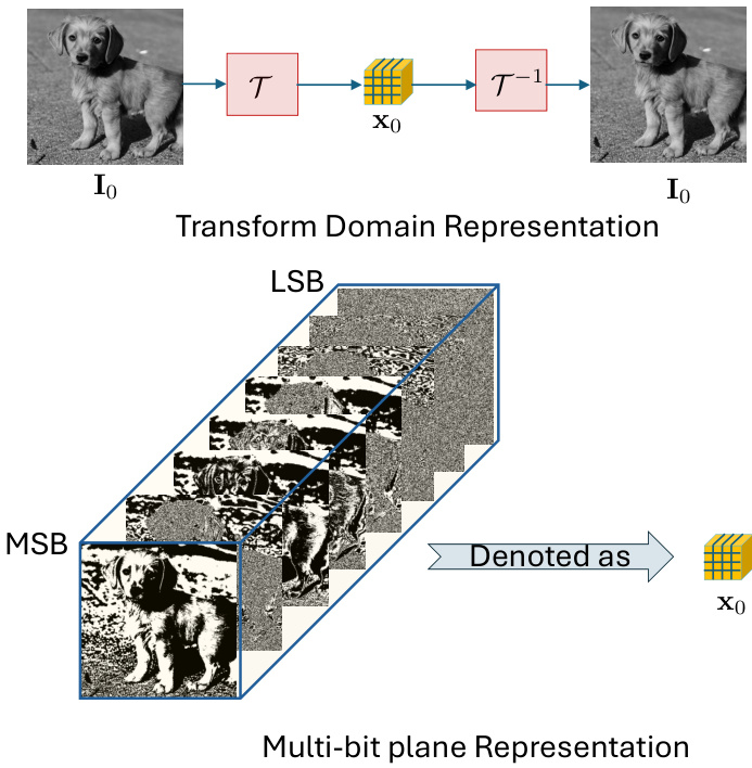
Figure 1. Multi-bit plane representation of images. An image ${\bf{I}}{0}$ is represented by $\mathbf{x}{0}$ through a bijective transform $\tau$ . In this work, $\tau$ decomposes the input image into bitplanes, organized within the tensor $\mathbf{x}{0}$ , where MSB planes capture the most significant bits and LSB planes capture the least significant bits. Notably, these representations are binary, satisfying $\begin{array}{r}{\mathbf I_{0}=\sum_{k=0}^{n-1}\mathbf x_{0}(k)2^{k}}\end{array}$ for a gray-scale image or RGB competent of a c olor image. The MSB planes exhibit high pixel correlation, while the LSB planes display greater independence across pixels.
图 1: 图像的多比特平面表示。图像 ${\bf{I}}{0}$ 通过双射变换 $\tau$ 表示为 $\mathbf{x}{0}$ 。本工作中,$\tau$ 将输入图像分解为比特平面,并组织在张量 $\mathbf{x}{0}$ 中,其中最高有效位(MSB)平面捕获最高有效比特,最低有效位(LSB)平面捕获最低有效比特。值得注意的是,这些表示是二进制的,满足灰度图像或彩色图像RGB分量的 $\begin{array}{r}{\mathbf I_{0}=\sum_{k=0}^{n-1}\mathbf x_{0}(k)2^{k}}\end{array}$ 。MSB平面表现出较高的像素相关性,而LSB平面则显示像素间更强的独立性。
Each bit plane captures unique statistical traits of the original image: the most significant bits (MSB) display stronger pixel correlations, while the least significant bits (LSB) are more independent. This layered structure allows precise noise control in the diffusion process, enhancing denoising and optimizing interpret ability, computational complexity, accuracy, and efficiency. We use this multi-bit plane representation, shown in Figure 1, to streamline and improve the generative model.
每个位平面都捕捉了原始图像独特的统计特征:最高有效位(MSB)表现出更强的像素相关性,而最低有效位(LSB)则更为独立。这种分层结构能够在扩散过程中实现精确的噪声控制,从而提升去噪效果,并优化可解释性、计算复杂度、准确性和效率。我们采用如图1所示的多位平面表示法来简化和改进生成模型。
3.2. Binary Diffusion Probabilistic Model
3.2. 二元扩散概率模型
BDPM shown in Figure 2 is a novel approach for generative modeling that leverages the simplicity of binary data representations. This method involves adding noise through XOR operation, which makes it particularly well-suited for handling binary data. Below, we describe the key aspects of the BDPM methodology in detail.
图 2 所示的 BDPM 是一种利用二进制数据表示简洁性的新型生成建模方法。该方法通过异或 (XOR) 运算添加噪声,使其特别适合处理二进制数据。下面我们将详细描述 BDPM 方法的关键方面。
In BDPM noise is added to the data by flipping bits using the XOR operation as defined by the mapper $\mathcal{M}{t}$ at each step $t$ . The amount of noise added is quantified by the proportion of bits flipped. Let $\mathbf{x}{0}(k)\in{0,1}^{h\times w}$ with $k=0,...,n-1$ for each color competent of the color image be the original binary bit-plane of dimension $h\times w$ , and $\mathbf{z}{t}(k)\in{0,1}^{h\times w}$ be a random binary noise plane at time step $t$ . The noisy bit plane ${\bf x}{t}(k)$ at the output of $\mathcal{M}{t}$ is obtained as: ${\bf x}{t}(k)={\bf x}{0}(k)\oplus{\bf z}{t}(k)$ , where $\bigoplus$ denotes the XOR operation. The noise level is defined as the fraction of bits flipped in $\mathbf{z}{t}(k)$ in the mapper $\mathcal{M}_{t}$ at step $t$ , with the number of bits flipped ranging within the probability range $[0,0.5]$ as a function of the timestep and potentially as a function of $k$ .
在BDPM中,噪声通过异或(XOR)运算按映射器$\mathcal{M}{t}$在每个步骤$t$对数据进行位翻转操作来添加。噪声量通过翻转位的比例来量化。设$\mathbf{x}{0}(k)\in{0,1}^{h\times w}$(其中$k=0,...,n-1$对应彩色图像的每个颜色分量)为原始$h\times w$维二元位平面,$\mathbf{z}{t}(k)\in{0,1}^{h\times w}$为时间步$t$的随机二元噪声平面。映射器$\mathcal{M}{t}$输出的含噪位平面${\bf x}{t}(k)$可表示为:${\bf x}{t}(k)={\bf x}{0}(k)\oplus{\bf z}{t}(k)$,其中$\bigoplus$表示异或运算。噪声水平定义为步骤$t$时映射器$\mathcal{M}{t}$中$\mathbf{z}_{t}(k)$的位翻转比例,其翻转位数作为时间步的函数(可能也与$k$相关)在概率范围$[0,0.5]$内变化。
The denoising network $g_{\theta}^{B}(\mathbf{x}{t},t,\mathbf{y}{e})$ is trained to predict both the added noise tensor of bit planes $\mathbf{z}{t}$ and the clean tensor of image bit planes $\mathbf{x}{\mathrm{0}}$ from the noisy tensor $\mathbf{x}_{t}$ . We employ binary cross-entropy (BCE) loss for each bit plane to train the denoising network. The loss function is averaged over the batch of $M$ samples:
去噪网络 $g_{\theta}^{B}(\mathbf{x}{t},t,\mathbf{y}{e})$ 被训练用于从含噪张量 $\mathbf{x}{t}$ 中同时预测位平面添加的噪声张量 $\mathbf{z}{t}$ 和图像位平面的干净张量 $\mathbf{x}_{\mathrm{0}}$。我们采用二元交叉熵 (BCE) 损失函数对每个位平面进行训练,该损失函数在批次大小为 $M$ 的样本上取平均值:
$$
\mathcal{L}(\boldsymbol{\theta})=\frac{1}{B}\sum_{m=1}^{M}\left[\mathcal{L}{x}(\hat{\mathbf{x}}{0}^{(m)},\mathbf{x}{0}^{(m)})+\mathcal{L}{z}(\hat{\mathbf{z}}{t}^{(m)},\mathbf{z}_{t}^{(m)})\right],
$$
$$
\mathcal{L}(\boldsymbol{\theta})=\frac{1}{B}\sum_{m=1}^{M}\left[\mathcal{L}{x}(\hat{\mathbf{x}}{0}^{(m)},\mathbf{x}{0}^{(m)})+\mathcal{L}{z}(\hat{\mathbf{z}}{t}^{(m)},\mathbf{z}_{t}^{(m)})\right],
$$
where $\theta$ represents the parameters of the denoising network, x $\mathbf{x}{0}^{(m)}$ and $\hat{\mathbf{x}}{0}^{(m)}$ are the $m$ -th samples of the true clean tensors and the predicted clean tensors, respectively. Similarly, zt $\mathbf{z}{t}^{(m)}$ and z(m) are the $m$ -th samples of the true added noise tensors and the predicted noise tensors, respectively. $\mathbf{y}{e}=\mathcal{E}{y}(\mathbf{I}{y})$ denotes the encoded conditional image $\mathbf{I}{y}$ that can represent the low-resolution down-sampled image, blurred image or image with removed parts that should be in-painted. The losses $\mathcal{L}{x}$ and $\mathcal{L}_{z}$ denote BCE losses computed for each bit plane $k$ and the pixel coordinates $i\in{1,\cdots,h}$ and $j\in{1,\cdots,w}$ withing each bit plane.
其中 $\theta$ 表示去噪网络的参数,$\mathbf{x}{0}^{(m)}$ 和 $\hat{\mathbf{x}}{0}^{(m)}$ 分别是真实干净张量和预测干净张量的第 $m$ 个样本。类似地,$\mathbf{z}{t}^{(m)}$ 和 $\mathbf{z}^{(m)}$ 分别是真实添加噪声张量和预测噪声张量的第 $m$ 个样本。$\mathbf{y}{e}=\mathcal{E}{y}(\mathbf{I}{y})$ 表示编码后的条件图像 $\mathbf{I}{y}$,可以代表低分辨率下采样图像、模糊图像或需要修复的部分缺失图像。损失函数 $\mathcal{L}{x}$ 和 $\mathcal{L}_{z}$ 表示针对每个位平面 $k$ 以及每个位平面内像素坐标 $i\in{1,\cdots,h}$ 和 $j\in{1,\cdots,w}$ 计算的 BCE (二元交叉熵) 损失。
In order to balance bit-planes during training of the denoiser network, we apply linear bit-plane weighting, where the weight for MSB is set to 1, weight for LSB is set to 0.1 and for others weights are linearly interpolated between 1 and 0.1. This fine-grained weighting can not be achieved with the MSE loss in a tractable form.
为了在去噪网络训练过程中平衡位平面,我们采用了线性位平面加权方法,其中最高有效位(MSB)的权重设为1,最低有效位(LSB)的权重设为0.1,其余位平面的权重则在1和0.1之间线性插值。这种细粒度加权无法通过均方误差(MSE)损失以可行形式实现。
The output of the denoiser $g_{\theta}^{B}(\mathbf{x}{t},t,\mathbf{y}_{e})$ is binarized via a mapper $\mathcal{Q}$ prior to applying the inverse transform $\tau^{-1}$ as shown in Figure 2.
去噪器的输出 $g_{\theta}^{B}(\mathbf{x}{t},t,\mathbf{y}_{e})$ 在应用逆变换 $\tau^{-1}$ 之前,会通过映射器 $\mathcal{Q}$ 进行二值化处理,如图 2 所示。
When sampling (Figure 2 right), we start from a random binary tensor $\mathbf{x}{t}$ at timestep $t=T$ , along with the conditioning state $\mathbf{I}{y}$ , encoded into ${\bf y}{e}$ . For each selected timestep in the sequence ${T,\ldots,0}$ , denoising is applied to the tensor. The denoised tensor $\hat{\mathbf{x}}{0}$ and the estimated binary noise $\hat{\mathbf{z}}{t}$ are predicted by the denoising network. These predictions are then processed using a sigmoid function and binarized with a threshold in the mapper $\mathcal{Q}$ . During sampling, we use the denoised tensor $\hat{\mathbf{x}}{0}$ directly. Then, random noise $\mathbf{z}{t}$ is generated and added to $\hat{\mathbf{x}}_{0}$ via the XOR operation:
在采样阶段 (图 2 右),我们从时间步 $t=T$ 的随机二元张量 $\mathbf{x}{t}$ 开始,同时将条件状态 $\mathbf{I}{y}$ 编码为 ${\bf y}{e}$。对于序列 ${T,\ldots,0}$ 中的每个选定时间步,对张量进行去噪处理。去噪网络预测出去噪后的张量 $\hat{\mathbf{x}}{0}$ 和估计的二元噪声 $\hat{\mathbf{z}}{t}$。这些预测结果通过sigmoid函数处理,并在映射器 $\mathcal{Q}$ 中用阈值进行二值化。采样过程中,我们直接使用去噪后的张量 $\hat{\mathbf{x}}{0}$。随后生成随机噪声 $\mathbf{z}{t}$,并通过XOR运算将其添加到 $\hat{\mathbf{x}}_{0}$ 中:
$\mathbf{x}{t}=\hat{\mathbf{x}}{0}\oplus\mathbf{z}_{t}$ . The sampling algorithm is summarized in Algorithm 1.
$\mathbf{x}{t}=\hat{\mathbf{x}}{0}\oplus\mathbf{z}_{t}$。采样算法如算法1所示。
Algorithm 1 Sampling algorithm.
算法 1: 采样算法
4. Experimental results
- 实验结果
We evaluate the proposed method on the following tasks: $4\times$ super-resolution task that scales images from $64\times64$ to $256\times256$ pixels using the FFHQ [19] and CelebA [27] datasets, medium size mask inpainting using FFHQ of the size $512\times512$ pixels, CelebA of the size $256\times256$ pix-els, CelebA-HQ [18] of the size $512\times512$ and blind image restoration on CelebA of the size $256\times256$ .
我们在以下任务上评估所提出的方法:使用FFHQ [19]和CelebA [27]数据集进行的4倍超分辨率任务(将图像从64×64放大到256×256像素)、在512×512像素FFHQ和256×256像素CelebA上执行的中等尺寸掩码修复、512×512像素CelebA-HQ [18]的修复任务,以及256×256像素CelebA上的盲图像恢复任务。
In all experiments, we use the same U-Net denoising model with 35.8M parameters, with 4 convolution downsampling blocks, self-attention[40] in the bottom downsampling block, and linear attention[20] in other down sampling blocks.
在所有实验中,我们使用相同的U-Net去噪模型(参数规模35.8M),包含4个卷积下采样块:底层下采样块采用自注意力(self-attention)[40],其余下采样块采用线性注意力(linear attention)[20]。
4.1. Datasets
4.1. 数据集
We perform experiments on three datasets: CelebA [27], FFHQ [19], and CelebA-HQ[18]. CelebA contains 202,599 celebrity images at a resolution of approximate ll y $178\times218$ pixels, each annotated with 40 facial attributes, we use train split for training and test split for evaluation. FFHQ consists of 70,000 high-quality face images at $1024\times1024$ resolution, offering diverse variations in age, ethnicity, and background. For all experiments, we split FFHQ into $60{,}000\mathrm{im}.$ - ages for training and 10,000 for evaluation. CelebA-HQ is a high-quality version of CelebA, comprising 30,000 images at $1024\times1024$ resolution. For the super-resolution task, we utilize CelebA and FFHQ datasets. The inpainting task employs all three datasets: CelebA, FFHQ, and CelebAHQ. For blind image restoration, our model is pretrained on FFHQ and evaluated on CelebA.
我们在三个数据集上进行实验:CelebA [27]、FFHQ [19] 和 CelebA-HQ [18]。CelebA 包含 202,599 张分辨率约为 $178\times218$ 像素的名人图像,每张图像标注了 40 个面部属性,我们使用训练集进行训练,测试集进行评估。FFHQ 由 70,000 张 $1024\times1024$ 分辨率的高质量人脸图像组成,涵盖了年龄、种族和背景的多样性。在所有实验中,我们将 FFHQ 分为 60,000 张训练图像和 10,000 张评估图像。CelebA-HQ 是 CelebA 的高质量版本,包含 30,000 张 $1024\times1024$ 分辨率的图像。对于超分辨率任务,我们使用 CelebA 和 FFHQ 数据集。修复任务则使用了全部三个数据集:CelebA、FFHQ 和 CelebA-HQ。在盲图像复原任务中,我们的模型先在 FFHQ 上预训练,然后在 CelebA 上进行评估。
Table 1. Comparsion of super-resolution approaches on FFHQ dataset. The best metrics are shown in bold and second best underscored.
表 1: FFHQ数据集上超分辨率方法的对比。最佳指标以粗体显示,次佳指标以下划线标示。
| 方法 | FID | LPIPS | PSNR | SSIM | NFEs |
|---|---|---|---|---|---|
| HiFaceGAN[48] | 5.36 | - | 28.65 | 0.816 | 1 |
| DPS [6] | 39.35 | 0.214 | 25.67 | 0.852 | 1000 |
| DDRM [21] | 62.15 | 0.294 | 25.36 | 0.835 | 1000 |
| DiffPIR [58] | 58.02 | 0.187 | 29.17 | 20 | |
| DiffPIR | 47.8 | 0.174 | 29.52 | 100 | |
| BDPM (ours) | 5.71 | 0.151 | 30.05 | 0.864 | 30 |
4.2. Metrics
4.2. 指标
We evaluate the model performance using Fréchet Inception Distance (FID) [13], Learned Perceptual Image Patch Similarity (LPIPS) [53], Peak Signal-to-Noise Ratio (PSNR), Structural Similarity Index Measure (SSIM) [45], and the number of function evaluations (NFEs), which corresponds to the number of model executions on the studied downstream tasks. Perceptual Image Defect Similarity (P-IDS), Unweighted Image Defect Similarity (U-IDS) [54] are also added to inpaiting evaluation.
我们使用Fréchet Inception距离(FID) [13]、学习感知图像块相似度(LPIPS) [53]、峰值信噪比(PSNR)、结构相似性指数(SSIM) [45]以及函数评估次数(NFEs)来评估模型性能,其中NFEs对应模型在所研究下游任务上的执行次数。感知图像缺陷相似度(P-IDS)和无权重图像缺陷相似度(U-IDS) [54]也被加入图像修复评估中。
4.3. Super-resolution
4.3. 超分辨率
The super-resolution process downscales the original $256\times$ 256 images by selecting every fourth pixel, then upsamples them back to $256\times256$ using bilinear interpolation. This upsampled image serves as the conditioning $\mathbf{I}_{y}$ (see Figure 2). The images are transformed into bitplanes via $\tau$ and concatenated with the input channels for the denoiser network. For super-resolution, we fix the diffusion steps at 30. Examples of ground truth, low-resolution inputs, and BDPM-upsampled images appear in Figure 3, with more examples and per-pixel variance shown in the Supplementary Materials.
超分辨率处理通过每隔四个像素选取一个的方式将原始 $256\times$ 256 图像降采样,随后使用双线性插值将其上采样回 $256\times256$ 尺寸。上采样后的图像作为条件输入 $\mathbf{I}_{y}$ (见图 2)。图像通过 $\tau$ 转换为比特平面,并与去噪网络的输入通道拼接。对于超分辨率任务,我们将扩散步数固定为 30。真实值、低分辨率输入和 BDPM 上采样图像的示例如图 3 所示,更多示例及逐像素方差见补充材料。
BDPM model is compared against SOTA GAN-based: HiFaceGAN [48] and diffusion-based methods: DPS [6], DDRM [21], and DiffPIR [58] on FFHQ dataset. On the FFHQ dataset, results are sumarized in Table 1, BDPM achieves superior results in LPIPS, PSNR, and SSIM metrics compared to previous approaches. On CelebA BDPM is compared against SOTA GAN-based models: PULSE [30], diffusion-based models: ILVR [5], DDNM [44], DiffFace [22], ResShift [51], DiT-SR [4] and transformer-based models: VQFR [11], CodeFormer [56], results are sumarized in Table 2, BDPM outperforms other methods in FID, LPIPS, and PSNR metrics.
在FFHQ数据集上,将BDPM模型与基于GAN的SOTA方法HiFaceGAN [48]以及基于扩散的方法DPS [6]、DDRM [21]和DiffPIR [58]进行对比。如表1所示,BDPM在LPIPS、PSNR和SSIM指标上均优于先前方法。在CelebA数据集上,BDPM与基于GAN的SOTA模型PULSE [30]、基于扩散的模型ILVR [5]、DDNM [44]、DiffFace [22]、ResShift [51]、DiT-SR [4]以及基于Transformer的模型VQFR [11]、CodeFormer [56]进行对比。如表2所示,BDPM在FID、LPIPS和PSNR指标上超越其他方法。
4.4. Inpainting
4.4. 图像修复
The inpainting problem involves reconstructing missing (masked) regions in images.
修复问题涉及重建图像中缺失(被遮挡)的区域。
In our approach, we use medium size masks, that mask between 10% and 30% of the total image size. In our approach, the masked image $\mathbf{I}{m}$ is transformed into bitplanes, and the missing pixels are replaced with random binary values ${0,1}$ . The mask is also provided to the denoiser network, and both the masked image and the mask are concatenated along the channel dimension as input to the model, e.g., $\mathbf{I}{y}=[\mathbf{M},\mathbf{I}{m}]$ , where M is inpainting mask and ${\bf{I}}_{m}$ is masked image. For the inpatining task, we fix the number of diffusion steps to 100. Examples of ground truth, masked images and inpainted by BDPM images are shown in Figure 4. More examples of inpainted images are presented in Supplementary material.
在我们的方法中,我们使用中等大小的掩码,覆盖图像总尺寸的10%到30%。该方法将掩码图像$\mathbf{I}{m}$转换为位平面,缺失像素用随机二进制值${0,1}$替代。掩码同时提供给去噪网络,掩码图像与掩码沿通道维度拼接后作为模型输入,即$\mathbf{I}{y}=[\mathbf{M},\mathbf{I}{m}]$(其中M为修复掩码,${\bf{I}}_{m}$为掩码图像)。修复任务中,我们将扩散步数固定为100步。图4展示了真实图像、掩码图像及经BDPM修复的示例结果,更多修复样本见补充材料。
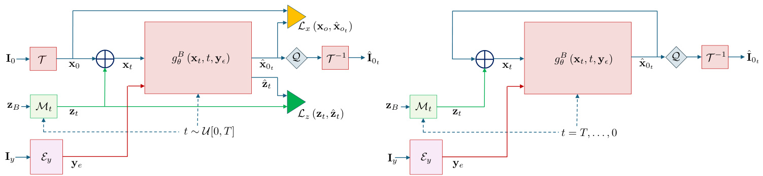
Figure 2. Binary Diffusion training (left) and sampling (right) schemes.
图 2: 二元扩散训练 (左) 与采样 (右) 流程示意图。
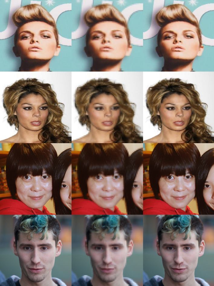
Figure 3. Super-resolution samples. First column: ground truth high-resolution samples, second column: low-resolution 4 times down-sampled samples, third column: samples reconstructed by BDPM model. First and second rows are from CelebA dataset, third and forth rows are from FFHQ dataset.
图 3: 超分辨率样本。第一列:真实高分辨率样本,第二列:4倍降采样的低分辨率样本,第三列:BDPM模型重建样本。前两行来自CelebA数据集,后两行来自FFHQ数据集。
Table 2. Comparsion of super-resolution approaches CelebA dataset. The best metrics are shown in bold and second best underscored. If the evaluation metric is not available in the paper, or in available public benchmark, it is marked as ‘-‘.
表 2: CelebA数据集超分辨率方法对比。最优指标以粗体显示,次优指标以下划线标注。若论文或公开基准测试中未提供评估指标,则标记为"-"。
| 方法 | FID | LPIPS | PSNR | SSIM | NFEs |
|---|---|---|---|---|---|
| PULSE [30] | 40.33 | 22.74 | 0.623 | 100 | |
| DDRM [21] | 31.04 | 31.04 | 0.941 | 100 | |
| ILVR [5] | 29.82 | - | 31.59 | 0.943 | 100 |
| VQFR [11] | 25.24 | 0.411 | 1 | 1 | |
| CodeFormer[56] | 26.16 | 0.324 | 1 | ||
| DiffFace [22] | 23.21 | 0.338 | - | 100 | |
| DDNM [44] | 22.27 | - | 31.63 | 0.945 | 100 |
| ResShift [51] | 17.56 | 0.309 | 1 | 4 | |
| DiT-SR [4] | 19.65 | 0.337 | 4 | ||
| BDPM (ours) | 3.5 | 0.116 | 32.01 | 0.91 | 30 |
We compare BDPM against the state-of-the-art methods: LaMa [39], CoModGAN [54], TFill [55], and SHGAN [47] on FFHQ, results are summarized in Table 3, BDPM outperforms consifered methods on FID, PSNR, SSIM, P-IDS and U-IDS metrics.
我们将BDPM与最先进的方法进行比较:LaMa [39]、CoModGAN [54]、TFill [55]和SHGAN [47]在FFHQ上的结果总结在表3中,BDPM在FID、PSNR、SSIM、P-IDS和U-IDS指标上优于所考虑的方法。
On the CelebA dataset, BDPM is compared against SOTA GAN-based methods: RePaint [29], EdgeConnect [31], DeepFillV2 [49], LaMa [39], diffusion-based methods: DDRM [21], DDNM [44] and transformer-based methods: ICT [41], MAT [25], results are sumarized in Table 4, BDPM achieves superior results on perceptual met- rics such as FID, P-IDS, and U-IDS.
在CelebA数据集上,BDPM与基于GAN的SOTA方法(RePaint [29]、EdgeConnect [31]、DeepFillV2 [49]、LaMa [39])、基于扩散的方法(DDRM [21]、DDNM [44])以及基于Transformer的方法(ICT [41]、MAT [25])进行了对比,结果汇总于表4。BDPM在FID、P-IDS和U-IDS等感知指标上取得了更优的结果。
For the CelebA-HQ dataset, we use the model pretrained on FFHQ and evaluate it on 10,000 randomly selected images. BDPM is compared against SOTA GANbased methods: Edge Connect [31], DeepFillv2 [49], AOT GAN [52], MADF [57], LaMa [39], CoModGAN [54] and transformer-based methods: ICT [39], MAT [25], results are sumarized in Table 5, BDPM surpasses current SOTA on perceptual metrics FID and LPIPS.
对于CelebA-HQ数据集,我们使用在FFHQ上预训练的模型,并在随机选择的10,000张图像上进行评估。BDPM与基于GAN的SOTA方法:Edge Connect [31]、DeepFillv2 [49]、AOT GAN [52]、MADF [57]、LaMa [39]、CoModGAN [54]以及基于Transformer的方法:ICT [39]、MAT [25]进行了比较,结果总结在表5中,BDPM在感知指标FID和LPIPS上超越了当前的SOTA。
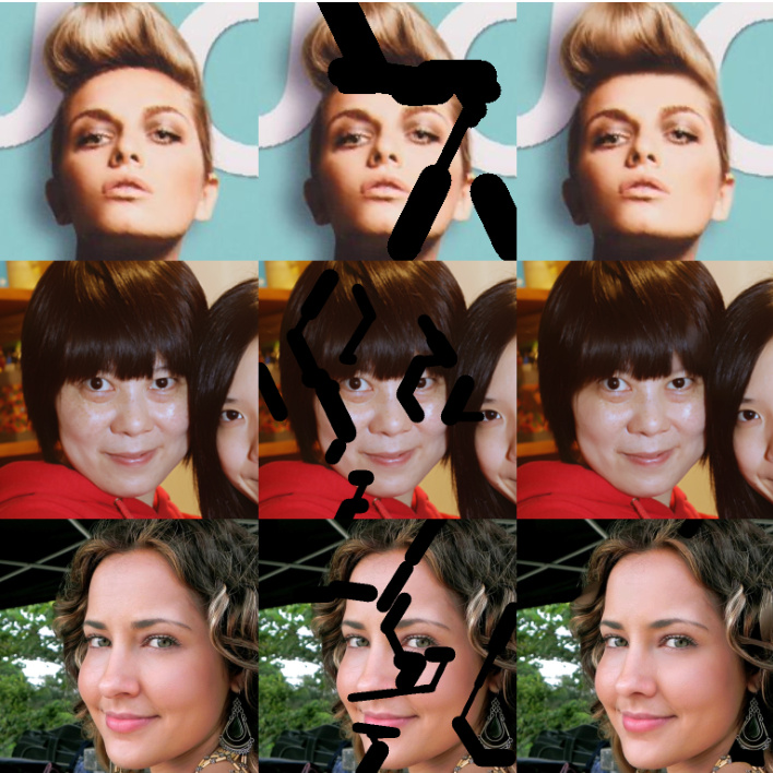
Figure 4. Inpainting samples. First column: ground truth highresolution sample, second row: masked sample, third row: inpainted by BDPM model. First row: CelebA dataset, second row: FFHQ dataset, third row: CelebA dataset.
图 4: 修复样本示例。第一列:真实高分辨率样本,第二列:掩码样本,第三列:经BDPM模型修复后的结果。第一行:CelebA数据集,第二行:FFHQ数据集,第三行:CelebA数据集。
Table 3. Comparison of inpainting approaches FFHQ dataset. The best metrics are shown in bold and second best underscored. If the evaluation metric is not available in the paper, or in available public benchmark, it is marked as ‘-‘.
表 3: FFHQ数据集上修复方法的对比。最佳指标以粗体显示,次佳指标以下划线标注。若论文或公开基准中未提供评估指标,则标记为"-"。
| 方法 | FID | LPIPS | PSNR | SSIM | P-IDS | U-IDS | NFEs |
|---|---|---|---|---|---|---|---|
| LaMa[39] | 19.6 | 0.287 | 18.99 | 0.7178 | - | - | 1 |
| CoModGAN[54] | 3.7 | 0.247 | 18.46 | 0.6956 | 16.6 | 29.4 | 1 |
| TFill[55] | 3.5 | 0.053 | " | - | - | - | 1 |
| SH-GAN[47] | 3.4 | 0.245 | 18.43 | 0.6936 | - | - | 1 |
| BDPM (ours) | 1.3 | 0.059 | 28.7 | 0.961 | 17.43 | 33.07 | 100 |
Table 4. Comparsion of inpainting approaches CelebA dataset. The best metrics are shown in bold and second best underscored. If the evaluation metric is not available in the paper, or in available public benchmark, it is marked as ‘-‘.
表 4: CelebA数据集上修复方法的对比。最佳指标以粗体显示,次佳指标以下划线标注。若论文或公开基准测试中未提供评估指标,则标记为"-"。
| 方法 | FID | LPIPS | PSNR | SSIM | P-IDS | U-IDS | NFEs |
|---|---|---|---|---|---|---|---|
| RePaint[29] | 14.19 | - | 35.2 | 0.981 | - | - | 2500 |
| DDRM[21] | 12.53 | - | 34.79 | 0.982 | - | - | 100 |
| EdgeConnect[31] | 12.16 | - | - | - | 0.84 | 2.31 | 1 |
| DeepFillV2[49] | 13.23 | - | - | - | 0.84 | 2.62 | 1 |
| ICT[41] | 10.92 | - | - | - | 0.9 | 5.23 | 1 |
| LaMa[39] | 8.75 | - | - | - | 2.34 | 8.77 | 1 |
| MAT[25] | 5.16 | - | - | - | 13.9 | 25.13 | 1 |
| DDNM[44] | 4.54 | - | 35.64 | 0.982 | - | - | 100 |
| BDPM (ours) | 1.96 | 0.08 | 28.3 | 0.928 | 15.04 | 27.01 | 100 |
4.5. Blind image restoration
4.5. 盲图像复原
Blind image restoration aims to recover high-quality images from degraded inputs without knowing the specific degradation. This task is challenging due to varied degradation s. To address this, we pretrain our BDPM model on a synthetic blind image restoration dataset from FFHQ images at $256\times256$ resolution, applying random combinations of perturbations. Details on these perturbations and parameters are in the Supplementary Materials, with examples of ground truth, perturbed, and restored images shown in Figure 5.
盲图像恢复旨在不知道具体退化类型的情况下,从退化的输入中恢复高质量图像。由于退化类型多样,这项任务具有挑战性。为此,我们在FFHQ图像合成的盲图像恢复数据集上预训练了BDPM模型(分辨率$256\times256$),并应用了随机组合的扰动。关于这些扰动和参数的详细信息见补充材料,真实图像、扰动图像和恢复图像的示例如图5所示。
Table 5. Comparsion of inpainting approaches CelebA-HQ dataset. The best metrics are shown in bold and second best underscored. If the evaluation metric is not available in the paper, or in available public benchmark, it is marked as ‘-‘.
表 5: CelebA-HQ数据集上不同修复方法的对比。最佳指标以粗体显示,次佳指标以下划线标注。若论文或公开基准测试中未提供评估指标,则标记为"-"。
| 方法 | FID | LPIPS | PSNR | SSIM | P-IDS | U-IDS | NFEs |
|---|---|---|---|---|---|---|---|
| EdgeConnect [31] | 10.58 | 0.101 | - | - | 4.14 | 12.45 | 1 |
| DeepFillv2 [49] | 10.11 | 0.117 | - | - | 3.11 | 9.52 | 1 |
| AOT GAN[52] | 4.65 | 0.074 | - | - | 7.92 | 20.45 | 1 |
| MADF [57] | 3.39 | 0.068 | - | - | 12.06 | 24.61 | 1 |
| ICT [41] | 6.28 | 0.105 | - | - | 2.24 | 9.99 | 1 |
| LaMa [39] | 4.05 | 0.075 | - | - | 9.72 | 21.57 | 1 |
| CoModGAN[54] | 3.26 | 0.073 | - | - | 19.95 | 31.41 | 1 |
| MAT [25] | 2.86 | 0.065 | - | - | 21.15 | 32.56 | 1 |
| BDPM (ours) | 1.17 | 0.06 | 29.41 | 0.925 | 14.14 | 28.4 | 100 |

Figure 5. Blind image restoration samples from CelebA dataset. First column: ground truth high-resolution sample, second row: degraded sample, third row: restored by BDPM model.
图 5: 来自CelebA数据集的盲图像修复样本。第一列:真实高分辨率样本,第二行:退化样本,第三行:经BDPM模型修复后的结果。
In our experiments, we fix the number of sampling steps for BDPM to 40. The BDPM model is compared against the state-of-the-art methods including CodeFormer [56], DR2 [46], BFRFormer [10], DiffBIR [26], GFP-GAN [43], BFRfusion [3], StableSR [42], and DifFace [50], results are sumarized in Table 6, BDPM achieves superior performance on metrics such as FID and SSIM.
在我们的实验中,我们将BDPM的采样步数固定为40。BDPM模型与当前最先进的方法进行了比较,包括CodeFormer [56]、DR2 [46]、BFRFormer [10]、DiffBIR [26]、GFP-GAN [43]、BFRfusion [3]、StableSR [42]和DifFace [50],结果总结在表6中,BDPM在FID和SSIM等指标上取得了更优的性能。
| 方法 | FID | LPIPS | PSNR | SSIM | NFEs |
|---|---|---|---|---|---|
| CodeFormer [56] | 60.62 | 0.299 | 22.18 | 0.61 | 1 |
| DR2 [46] | 58.94 | 0.3979 | 24.44 | 0.6784 | 250 |
| BFRFormer [10] | 57.37 | 0.27 | 22.83 | - | 1 |
| DiffBIR [26] | 47.9 | 0.3786 | 25.6 | 0.6809 | 50 |
| GFP-GAN [43] | 42.62 | 0.3646 | 25.08 | 0.6777 | 1 |
| BFRffusion [3] | 40.74 | 0.3621 | 26.2 | 0.6926 | 50 |
| StableSR [42] | 39.73 | 0.3637 | 24.84 | 0.6772 | 200 |
| DifFace [50] | 20.29 | 0.461 | 23.44 | 0.67 | 100 |
| BDPM (ours) | 12.93 | 0.293 | 24.58 | 0.7415 | 40 |
Table 6. Comparison of Bling Image Restoration on CelebA dataset. The best metrics are shown in bold and second best underscored. If the evaluation metric is not available in the paper, or in available public benchmark, it is marked as ‘-‘.
表 6: CelebA数据集上的盲图像恢复方法对比。最佳指标以粗体显示,次佳指标以下划线标注。若论文或公开基准测试中未提供评估指标,则标记为"-"。
4.6. Comparison with Posterior Sampling Methods
4.6. 与后验采样方法的对比
BDPM is compared to posterior sampling models such as DPS [6], DDRM [21], DiffPIR [58], DDNM [44], DiffBIR [26], BFRFusion [3], and StableSR [42] (see Tables 1, 2, 3, and 6). These methods leverage large pretrained diffusion models [8, 33] and adapt them for specific tasks using posterior sampling. Details on number of parameters for each model are provided in Supplementary Materials. Although these methods do not require additional training, they often need more sampling steps and rely on larger models for inference, making them less suitable for large-scale deployment. In contrast, the proposed method requires training but is compact with 35.8 million parameters and enables fast sampling. It outperforms posterior sampling methods, making it more suitable for large-scale applications.
BDPM 与 DPS [6]、DDRM [21]、DiffPIR [58]、DDNM [44]、DiffBIR [26]、BFRFusion [3] 和 StableSR [42] 等后验采样模型进行了对比 (见 表 1、表 2、表 3 和 表 6)。这些方法利用大型预训练扩散模型 [8, 33],并通过后验采样将其适配到特定任务。各模型参数量的详细信息见补充材料。虽然这些方法无需额外训练,但通常需要更多采样步骤且依赖更大模型进行推理,因此不太适合大规模部署。相比之下,本文提出的方法虽然需要训练,但模型紧凑 (仅 3580 万参数) 且支持快速采样,其性能优于后验采样方法,更适用于大规模应用场景。
4.7. Comparison with Gaussian Diffusion
4.7. 与高斯扩散的对比
To compare BDPM with the classical Gaussian DDPM model, we pre-trained both models for conditional image generation on the CIFAR-10 [24] dataset, using identical architectures except that BDPM accepts 24 input channels (3 color channels split into 8 bitplanes each). Both models were pre-trained for 200,000 iterations with a batch size of 256, the Adam optimizer [23], a constant learning rate of $10^{-4}$ , and EMA updates every 10 steps with a decay rate of $\beta=0.995$ . Classifier-free guidance [14] was applied before b inari z ation, with guidance scales of 3 for DDPM/DDIM [38] and 5 for BDPM. We generated 50,000 samples per model for each number of sampling steps. Figure 6 shows the relationship between sampling steps and FID for each model.
为比较BDPM与经典高斯DDPM模型的性能,我们在CIFAR-10[24]数据集上对两个模型进行了条件图像生成的预训练。两者采用相同架构,仅BDPM接受24个输入通道(将3个颜色通道各自拆分为8个位平面)。模型均以256的批量大小预训练200,000次迭代,使用Adam优化器[23],恒定学习率$10^{-4}$,每10步进行EMA更新(衰减率$\beta=0.995$)。二值化前应用无分类器引导[14],DDPM/DDIM[38]的引导尺度为3,BDPM为5。每个采样步数下各模型生成50,000个样本。图6展示了各模型的采样步数与FID的关系。
For a fair comparison, we evaluated BDPM against baseline DDPM and DDIM sampling methods. While future work will adapt samplers specifically for BDPM, this study focuses on comparing sampling trends across DDPM, DDIM, and BDPM.
为公平比较,我们针对基线DDPM和DDIM采样方法评估了BDPM。虽然未来工作将专门为BDPM适配采样器,但本研究重点在于比较DDPM、DDIM和BDPM之间的采样趋势。
Our results show that BDPM performs competitively with DDPM and DDIM in conditional image generation on the CIFAR-10 dataset, achieving convergence with fewer sampling steps under identical architectures and training conditions. Additional analysis is available in the Supplementary Materials.
我们的结果表明,在CIFAR-10数据集的条件图像生成任务中,BDPM与DDPM和DDIM表现相当,在相同架构和训练条件下能以更少的采样步骤实现收敛。补充材料中提供了更多分析。

Figure 6. Relationship between the FID metric and the number of sampling steps for conditional image generation on the CIFAR-10 dataset. As shown, BDPM’s FID saturates beyond a certain point, indicating no further improvement with additional sampling steps. While DDPM and DDIM achieve better results when sampling for 1,000 steps, BDPM exhibits a distinctive trend worth noticing, where bigger number of sampling steps do not lead to better generation in terms of FID.
图 6: CIFAR-10数据集上条件图像生成的FID指标与采样步数的关系。如图所示,BDPM的FID在超过某一点后趋于饱和,表明增加采样步数不会带来进一步改善。虽然DDPM和DDIM在1,000步采样时取得更好结果,但BDPM呈现出值得注意的独特趋势——更多采样步数并不会在FID指标上带来更好的生成效果。
5. Conclusions
5. 结论
In this work, we introduce the BDPM, a novel diffusionbased generative framework tailored for binary data representations. Unlike traditional DDPMs, which rely on continuous representations and Gaussian noise, BDPM utilizes a binary bit-plane approach with XOR-based noise transformations and binary cross-entropy loss. The model is specifically optimized for binary data, leading to improved efficiency and effectiveness across image restoration tasks.
在本工作中,我们提出了BDPM,这是一种专为二进制数据表示设计的新型基于扩散的生成框架。与依赖连续表示和高斯噪声的传统DDPM不同,BDPM采用二进制位平面方法,结合基于XOR的噪声变换和二元交叉熵损失。该模型针对二进制数据进行了专门优化,从而在图像修复任务中实现了更高的效率和效果。
Our experiments show that BDPM achieves state-of-theart performance in super-resolution, inpainting, and blind image restoration on datasets like FFHQ, CelebA, and CelebA-HQ. BDPM requires fewer inference steps than Gaussian-based models, underscoring its computational efficiency.
我们的实验表明,BDPM在FFHQ、CelebA和CelebA-HQ等数据集上的超分辨率、修复和盲图像恢复任务中实现了最先进的性能。与基于高斯(Gaussian)的模型相比,BDPM需要更少的推理步骤,凸显了其计算效率。
By using binary cross-entropy instead of traditional MSE loss, BDPM aligns better with the discrete nature of digital images, enhancing convergence and preserving binary data integrity for faster, stable training. BDPM’s compact size of 35.8M parameters also makes it well-suited for real-world applications with limited computational resources.
通过采用二元交叉熵而非传统的均方误差损失函数,BDPM能更好地契合数字图像的离散特性,从而提升收敛速度并保持二进制数据完整性,实现更快速稳定的训练。BDPM仅需3580万参数的紧凑规模,也使其特别适合计算资源有限的现实应用场景。
References
参考文献
Binary Diffusion Probabilistic Model
二元扩散概率模型
Supplementary Material
补充材料
6. Ablation studies
6. 消融实验
We perform the ablation study on the loss function. We pretrain 3 identical BDPMs for conditional image generation task on the CIFAR-10 [24] dataset with different losses: loss on added noise estimation $\mathcal{L}{z}(\hat{\mathbf{z}}{t}^{(m)},\mathbf{z}{t}^{(m)})$ , loss on image estimation $\mathcal{L}{x}(\hat{\mathbf{x}}{0}^{(m)},\mathbf{x}{0}^{(m)})$ and loss on both noise and image estimations $\begin{array}{r}{\mathcal{L}{x}(\hat{\mathbf{x}}{0}^{(m)},\mathbf{x}{0}^{(m)})+\mathcal{L}{z}(\hat{\mathbf{z}}{t}^{(m)},\mathbf{z}_{t}^{(m)})}\end{array}$ . Models were pre-trained for 200,000 iterations with a batch size of 256, using the Adam optimizer [23], a constant learning rate of $10^{-4}$ , and exponential moving average (EMA) updates every 10 steps with a decay rate of $\beta=0.995$ . During pre-training and sampling, we employed classifier-free guidance [14], applied before the b inari z ation step. Then we sample 50000 images for each model, using 50 sampling steps and guidance 5. Models are evaluated using FID metric. Results are summarized in Table 7. The best FID is achieved when using combination of two losses for the image and added noise estimation.
我们对损失函数进行了消融研究。在CIFAR-10 [24]数据集上预训练了3个相同的BDPM模型用于条件图像生成任务,分别采用不同损失函数:添加噪声估计损失$\mathcal{L}{z}(\hat{\mathbf{z}}{t}^{(m)},\mathbf{z}{t}^{(m)})$、图像估计损失$\mathcal{L}{x}(\hat{\mathbf{x}}{0}^{(m)},\mathbf{x}{0}^{(m)})$,以及噪声与图像联合估计损失$\begin{array}{r}{\mathcal{L}{x}(\hat{\mathbf{x}}{0}^{(m)},\mathbf{x}{0}^{(m)})+\mathcal{L}{z}(\hat{\mathbf{z}}{t}^{(m)},\mathbf{z}_{t}^{(m)})}\end{array}$。所有模型采用Adam优化器[23],批量大小为256,固定学习率$10^{-4}$,每10步执行一次衰减率$\beta=0.995$的指数移动平均(EMA)更新,共预训练200,000次迭代。预训练和采样阶段均在二值化步骤前应用无分类器引导[14]。每个模型使用50步采样和引导系数5生成50,000张图像,采用FID指标进行评估。结果如 表 7 所示,当联合使用图像和添加噪声的估计损失时,模型取得了最佳FID值。
Table 7. Loss function ablation study.
表 7: 损失函数消融研究
| 损失函数 | FID |
|---|---|
| C=(2(m) m Z | 17.88 |
| Lx(x(m), (m) x | 19.91 |
| La(x(m),x(m)+L=(2(m),z(m) | 13.85 |
7. Implementation details
7. 实现细节
Denoiser architecture and training parameters: We use PyTorch [1] and Accelerate [12] deep learning frameworks for both training and inference of the model. The U-Net denoiser network [34] is inspired by the denoiser from [8]. The U-Net denoiser consists of four convolutional downsampling blocks. The bottom down sampling block uses self-attention [40], while linear attention [20] is used in all layers except the last one. To accelerate training and inference, we incorporate Flash Attention [7] and bfloat16 precision. Our denoiser consists of 35.8 million parameters. Sinusoidal timestep conditioning [15] is integrated as biases in every block. Image conditioning (for tasks such as super-resolution, inpainting, and restoration) is appended as extra channels to the input. Vector conditioning (e.g., onehot encoded classes) is added as biases to every layer. We use the same training setup across all tasks. Specifically, we use EMA distillation for the denoiser model, and the EMA model is then used for evaluation purposes. During training, the denoiser predicts both the clean image’s bitplanes and the binary noise associated with each bitplane. At each timestep $t\in[0,T]$ , the amount of noise added to each bitplane remains constant. However, since different bitplanes hold varying levels of importance, we adopt a linearly interpolated weighting scheme for the binary cross-entropy loss. The most significant bitplane is assigned a weight of 1, while the least significant bitplane receives a weight of 0.1, with intermediate bitplanes assigned weights that are linearly interpolated between these values. This approach ensures that higher bitplanes, which contribute more to the image’s overall structure and quality, are prioritized during training. The weights for noise prediction are kept constant at 1 for each bitplane. We define the noise level as the fraction of bits flipped in $z_{t}(k)$ by the mapper $\mathcal{M}_{t}$ at step $t$ , with the number of bits flipped ranging within the probability range $[0,0.5]$ as a function of the timestep $t$ and potentially as a function of $k$ .
去噪器架构与训练参数:我们使用PyTorch [1]和Accelerate [12]深度学习框架进行模型的训练和推理。U-Net去噪网络[34]的设计灵感来源于[8]中的去噪器。该U-Net去噪器包含四个卷积下采样块,底层下采样块采用自注意力机制[40],其余层均使用线性注意力[20]。为加速训练和推理,我们整合了Flash Attention [7]技术与bfloat16精度。去噪器参数量为3580万,所有模块均采用正弦时间步条件编码[15]作为偏置项。图像条件输入(如超分辨率、修复和复原任务)以额外通道形式拼接至输入端,向量条件(例如onehot编码类别)则作为偏置项添加至每层。所有任务采用统一训练配置:通过EMA蒸馏训练去噪模型,最终评估使用EMA模型。训练时去噪器同时预测洁净图像的位平面及其对应二值噪声。在时间步$t\in[0,T]$中,每个位平面的噪声注入量恒定,但考虑到不同位平面重要性差异,我们对二元交叉熵损失采用线性插值加权方案——最高有效位平面权重为1,最低有效位平面权重0.1,中间位平面权重按线性插值分配。这种机制确保对图像结构和质量影响更大的高位平面在训练中获得更高优先级。噪声预测权重统一设为1。噪声水平定义为步骤$t$时映射器$\mathcal{M}{t}$对$z{t}(k)$的比特翻转比例,其翻转比特数在概率范围$[0,0.5]$内随时间步$t$变化,并可能随$k$值变化。
To control this noise level, we use quadratic noise scheduling for the diffusion process. The noise schedule $\beta_{t}$ at time step $t$ determines the probability of bits being flipped and is defined as:
为了控制这一噪声水平,我们在扩散过程中采用二次噪声调度。时间步 $t$ 的噪声调度 $\beta_{t}$ 决定了比特翻转概率,其定义为:
$$
\beta_{t}=\left(\sqrt{\beta_{\mathrm{start}}}+\frac{t}{T}\left(\sqrt{\beta_{\mathrm{end}}}-\sqrt{\beta_{\mathrm{start}}}\right)\right)^{2},
$$
$$
\beta_{t}=\left(\sqrt{\beta_{\mathrm{start}}}+\frac{t}{T}\left(\sqrt{\beta_{\mathrm{end}}}-\sqrt{\beta_{\mathrm{start}}}\right)\right)^{2},
$$
where $T$ is the total number of time steps (default is 1000), $\beta_{\mathrm{start}}$ is the minimum value of the noise, $10^{-5}$ by default, $\beta_{\mathrm{start}}$ is maximum value of the noise. $\beta_{t}$ controls the probability of the bit to be flipped.
其中 $T$ 是总时间步数 (默认为1000),$\beta_{\mathrm{start}}$ 是噪声最小值 (默认为 $10^{-5}$),$\beta_{\mathrm{start}}$ 是噪声最大值。$\beta_{t}$ 控制比特翻转概率。
The training parameters are summarized in Table 8.
训练参数总结如表 8:
Table 8. Training Hyper parameters
表 8: 训练超参数
| 超参数 | 值 |
|---|---|
| 优化器 | AdamW |
| 学习率 | 1 × 10⁻⁴ |
| 权重衰减 | 1 × 10⁻⁶ |
| 训练步数 | 500,000 |
| 梯度累积 | 否 |
| EMA更新频率 | 10步 |
| EMA衰减噪声计划 | 0.995 |
| Quadratic | |
| 扩散步数 | 1,000 |
| 图像位平面权重 | Linear |
| 掩码位平面权重 | Constant |
| 精度 | bfloat16 |
| 64(256×256图像) | |
| 批量大小 | 8(512×512图像) |
Super-Resolution Implementation: The conditioning is performed by concatenating the bitplanes of the bilinearly upsampled low-resolution image as extra channels. During training, we apply random cropping (ranging from $80%$ to $100%$ of the image height and width) and horizontal flipping as data augmentation techniques. For evaluation, we use the PSNR, SSIM, LPIPS, and FID metrics.
超分辨率实现:通过将双线性上采样的低分辨率图像的位平面作为额外通道进行拼接来实现条件化。训练过程中,我们采用随机裁剪(范围为图像高度和宽度的 $80%$ 至 $100%$)和水平翻转作为数据增强技术。评估时,我们使用 PSNR、SSIM、LPIPS 和 FID 指标。
Inpainting Implementation: The conditioning is performed by concatenating the bitplanes of masked images, where masked pixels are replaced with random noise. Additionally, the mask is concatenated to the input. During training, we apply random cropping (ranging from $80%$ to $100%$ of the image height and width) and horizontal flipping as data augmentation techniques. For evaluation, we use the PSNR, SSIM, LPIPS, FID, P-IDS, and U-IDS metrics.
修复(Inpainting)实现:通过将掩码图像的位平面与随机噪声替换的掩码像素进行拼接来实现条件输入。此外,掩码也会与输入拼接。训练过程中,我们采用随机裁剪(范围为图像高度和宽度的$80%$至$100%$)和水平翻转作为数据增强技术。评估时使用PSNR、SSIM、LPIPS、FID、P-IDS和U-IDS指标。
Blind Image Restoration Implementation: The conditioning is performed by concatenating the bitplanes of the perturbed image as extra channels. We pretrain our BDPM model on a synthetic blind image restoration dataset constructed from FFHQ images at a resolution of $256\times256$ . The degradation s are simulated by randomly applying a combination of perturbations to the images, summarized in Table 9.
盲图像恢复实现:通过将扰动图像的位平面作为额外通道进行拼接来实现条件化。我们在一个由FFHQ图像构建的合成盲图像恢复数据集上预训练了BDPM模型,分辨率为$256\times256$。通过随机对图像应用一系列扰动组合来模拟退化过程,具体总结如表9所示。
Table 9. Perturbations, Parameters, and Probabilities Used in the Degradation Process.
表 9: 退化过程中使用的扰动、参数及概率
| 扰动类型 | 参数 | 概率 |
|---|---|---|
| GaussianBlur | 核尺寸:21×21 | Always |
| 核类型:各向同性或各向异性 | ||
| Ox,Oy ∈ [0.1, 7] 旋转角度 ∈ [-π,π] | ||
| Downsampling | 缩放比例 [1, 4] | Always |
| AdditiveGaussianNoise | 标准差 [0,15]/255 | Always |
| JPEGCompression | 质量因子 [50,100] | Always |
| ColorShift | 每通道偏移量 [-20/255,20/255] | 30% |
| ColorJitter | 亮度 [0.5,1.5] | |
| 对比度 [0.5,1.5] | ||
| 饱和度 [0,1.5] | ||
| 色调 [0.1, 0.1] | ||
| GrayscaleConversion | 1% |
8. Number of parameters
8. 参数量
The experimental part of the main section used several stateof-the-art Gaussian DDPM. Table 10 summarizes the number of parameters in these models.
主体部分的实验采用了若干先进的Gaussian DDPM (Diffusion Denoising Probabilistic Models)。表 10 总结了这些模型的参数量。
9. Effect of number of sampling steps
9. 采样步骤数量的影响
9.1. CIFAR10 generation
9.1. CIFAR10 生成
Figure 7 show the CIFAR10 samples, generated by the BDPM model for different number of sampling steps:
图 7: 展示了由BDPM模型在不同采样步数下生成的CIFAR10样本:
Table 10. Number of parameters in compared models.
表 10: 对比模型的参数量
| 模型 | 参数量 |
|---|---|
| DDPM [21] | 554M |
| DPS [6] DiffPIR [58] | 554M 554M |
| DDNM [44] DiffBIR[26] BFRffusion[3] | 554M 17.2B 1.23B |
| StableSR[42] HiFaceGAN[48] | 1.20B 54M |
| PULSE [30] | 26.2M |
| ILVR [5] VQFR [11] | 554M |
| CodeFormer [56] | 76.3M |
| ResShift [51] | 74M |
| 118.6M | |
| DiT-SR [4] | |
| EdgeConnect [31] | 100.6M |
| DeepFillV2[49] | |
| 27M | |
| 4.1M | |
| AOTGAN[52] | |
| MADF [57] | 15.2M |
| ICT [39] | 85M |
| 120M | |
| LaMa [39] | |
| CoModGAN [54] | 51M |
| 109M | |
| MAT [25] | 62M |
| TFill [55] | 70M |
| SH-GAN[47] | 79.8M |
| RePaint [29] | 554M |
| DR2 [46] | 168M |
| GFP-GAN[43] | 56M |
| DifFace [50] | 176M |
| BDPM (ours) | 35.8M |
1000, 500, 250, 100, 50, 25. For every number of steps, we generate 10 samples for each class. We observe, that samples that are generated with larger number of sampling steps tend to be of better quality (less artifacts), but to be less diverse. For example, one can clearly see that for 1000 sampling steps in Figure 7 (a), for class airplane (first column), two samples (rows 3 and 8) look almost identical, the same can be observed for class track (last column), thress samples (rows 1, 3, 4) are almost identical. For smaller number of sampling steps, generated samples are more diverse, but they can be of lower quality (have most generated artifacts).
1000、500、250、100、50、25。对于每个采样步数,我们为每个类别生成10个样本。我们观察到,采样步数较多的样本往往质量更好(伪影更少),但多样性较低。例如,在图7(a)中,可以明显看到对于1000采样步数的飞机类别(第一列),有两个样本(第3行和第8行)看起来几乎相同,同样的情况也出现在卡车类别(最后一列),有三个样本(第1、3、4行)几乎相同。对于较少的采样步数,生成的样本多样性更高,但质量可能较低(生成的伪影较多)。
9.2. Image-to-image translation
9.2. 图像到图像转换
The similar trend, when BDPM with smaller number of steps achieves better results is shown with other generative tasks: super-resolution, inpainting and blind image restoration. For evaluation, we use the pretrained models on $256\times$ 256 FFHQ dataset. We show the relationship between number of sampling steps and evaluation metrics: FID, LPIPS, SSIM and PSNR. We evaluate model on 200 images for different number of sampling steps. The plots with relationship between the evaluation metrics and number of sampling steps are shows in the Figure 8. We select the optimal number of sampling steps, based on FID metric from evaluated 200 images for each of the tasks.
类似趋势也出现在其他生成任务中:超分辨率、图像修复和盲图像恢复,当BDPM采用较少步数时能获得更好结果。我们使用在$256\times$256 FFHQ数据集上预训练的模型进行评估,展示了采样步数与评估指标(FID、LPIPS、SSIM和PSNR)的关系。针对不同采样步数,我们在200张图像上进行模型评估。图8展示了评估指标与采样步数的关系曲线。基于每项任务在200张测试图像上的FID指标,我们选取了最优采样步数。

(f) 25 sampling steps Figure 7. CIFAR10 conditional image generation with different number of sampling steps using BDPM model. Each column has sample of the same class.
(f) 25 采样步数
图 7: 使用 BDPM 模型在不同采样步数下的 CIFAR10 条件图像生成结果。每列展示同类别样本。
10. Results
10. 结果
Figures 9,10 show super-resolution samples generated using BDPM for datasets FFHQ and CelebA respectively. Ground truth images are shown in the first column, low resolution images are shown in the second columns, highresolution image generated by BDPM, per-pixel variance over 10 high-resolution generations, per-pixel variances over 10 high-resolution generations are shown in the fourth columns.
图 9 和图 10 分别展示了使用 BDPM (Bidirectional Denoising Probabilistic Model) 在 FFHQ 和 CelebA 数据集上生成的超分辨率样本。第一列为真实图像,第二列为低分辨率图像,第三列为 BDPM 生成的高分辨率图像,第四列为 10 次高分辨率生成结果的逐像素方差。
Figures 11,12,13 show inpainting samples generated using BDPM for datasets FFHQ, CelebA and CelebA-HQ re- spectively. Masks are shown in the first row, ground truth images are shown in the first column, inpainting samples for each masks are shown in the columns 2 - 6.
图 11、12、13 分别展示了使用 BDPM 在 FFHQ、CelebA 和 CelebA-HQ 数据集上生成的修复样本。第一行显示掩码,第一列显示真实图像,第 2-6 列显示对应各掩码的修复样本。
Figure 14 shows blind image restortion results. Ground truth images are shown in the first column, perturbed images are shown in the second column, restored images are shown in columns 3 - 5.
图 14: 展示了盲图像复原结果。第一列为真实图像,第二列为扰动图像,第3-5列为复原图像。

Figure 8. Relationship between the evaluation metrics and number of sampling steps on super-resolution task on FFHQ $256\times256$
图 8: FFHQ $256\times256$ 超分辨率任务中评估指标与采样步数的关系

Figure 9. FFHQ super resolution $256~\times~256$ . First column: ground truth image, second column: low resolution image, third column: high-resolution image generated by BDPM, forth column: per-pixel variance over 10 high-resolution generations.
图 9: FFHQ 超分辨率 $256~\times~256$ 。第一列:真实图像,第二列:低分辨率图像,第三列:BDPM 生成的高分辨率图像,第四列:10 次高分辨率生成的逐像素方差。

Figure 10. CelebA super resolution $256\times256$ . First column: ground truth image, second column: low resolution image, third column: high-resolution image generated by BDPM, forth column: per-pixel variance over 10 high-resolution generations.
图 10. CelebA 超分辨率 $256\times256$ 。第一列:真实图像,第二列:低分辨率图像,第三列:BDPM 生成的高分辨率图像,第四列:10 次高分辨率生成的逐像素方差。

Figure 11. FFHQ inpainting $512\times512$ . First row: inpainting masks, first column: ground truth images, 2-6 columns: inpainting images generated by BDPM.
图 11. FFHQ 图像修复 $512\times512$ 。首行: 修复遮罩,首列: 真实图像,2-6列: 由BDPM生成的修复图像。

Figure 12. CelebA inpaint $256\times256$ . First row: inpainting masks, first column: ground truth images, 2-6 columns: inpainting images generated by BDPM.
图 12: CelebA 图像修复 $256\times256$ 。第一行:修复遮罩,第一列:真实图像,2-6列:由 BDPM 生成的修复图像。

Figure 13. CelebA-HQ inpaint $512\times512$ . First row: inpainting masks, first column: ground truth images, 2-6 columns: inpainting images generated by BDPM.
图 13. CelebA-HQ 图像修复 $512\times512$ 。第一行:修复遮罩,第一列:真实图像,2-6列:由BDPM生成的修复图像。

Figure 14. CelebA blind image restoration $256\times256$ . First column: ground truth images, second column: distorted images, 3-5 columns: images restored by BDPM.
图 14. CelebA 盲图像恢复 $256\times256$ 。第一列:真实图像,第二列:失真图像,3-5列:BDPM 恢复的图像。